Singapore Management UniversityInstitutional Knowledge at Singapore Management University

Research Collection School Of Economics School of Economics

8-2017

Competition, markups, and gains from trade: Aquantitative analysis of China between 1995 and2004Wen-Tai HSUSingapore Management University, WENTAIHSU@smu.edu.sg

Yi LU

Guiying Laura WU

Follow this and additional works at: http://ink.library.smu.edu.sg/soe_research

Part of the Asian Studies Commons, and the Management Sciences and Quantitative MethodsCommons

This Working Paper is brought to you for free and open access by the School of Economics at Institutional Knowledge at Singapore ManagementUniversity. It has been accepted for inclusion in Research Collection School Of Economics by an authorized administrator of Institutional Knowledgeat Singapore Management University. For more information, please email libIR@smu.edu.sg.

CitationHSU, Wen-Tai; LU, Yi; and WU, Guiying Laura. Competition, markups, and gains from trade: A quantitative analysis of Chinabetween 1995 and 2004. (2017). 1-67. Research Collection School Of Economics.Available at: http://ink.library.smu.edu.sg/soe_research/2078

Competition, Markups, and Gains from Trade: A Quantitative Analysis of China Between 1995

and 2004

Wen-Tai Hsu, Yi Lu, Guiying Laura Wu

August 2017

Paper No. 12-2017

ANY OPINION EXPRESSED ARE THOSE OF THE AUTHOR(S) AND NOT NECESSARILY THOSE OF THE SCHOOL OF ECONOMICS, SMU

Competition, Markups, and Gains from Trade: AQuantitative Analysis of China Between 1995 and

2004

Wen-Tai Hsu Yi Lu Guiying Laura Wu∗†

August 2, 2017

Abstract

This paper provides a quantitative analysis of gains from trade in a model with

head-to-head competition using Chinese firm-level data from Economic Censuses in

1995 and 2004. We find a significant reduction in trade cost during this period, and

total gains from such improved openness during this period is 9.4%. The gains are

decomposed into a Ricardian component and two pro-competitive ones. The pro-

competitive effects account for 25.4% of the total gains. Moreover, the total gains

from trade are 17 − 27% larger than what would result from the formula provided

by ACR (Arkolakis, Costinot, and Rodriguez-Clare 2012), which nests a class of im-

portant trade models, but without pro-competitive effects. We find that head-to-head

competition is the key reason behind the larger gains, as trade flows do not reflect

all of the effects via markups in an event of trade liberalization. One methodological

advantage of this paper’s quantitative framework is that its application is not con-

strained by industrial or product classifications; thus it can be applied to countries of

any size.

∗Hsu: School of Economics, Singapore Management University. 90 Stamford Road, Singapore 178903.Email: wentaihsu@smu.edu.sg; Lu: School of Economics and Management, Tsinghua University, Beijing100084, China. Email: luyi@sem.tsinghua.edu.cn; Wu: Division of Economics, School of Humanities andSocial Sciences, Nanyang Technological University. 14 Nanyang Drive, Singapore 637332. Email: guiy-ing.wu@ntu.edu.sg.†For their helpful comments, we thank Costas Arkolakis, Issac Baley, Pao-Li Chang, Davin Chor,

Jonathan Eaton, Tom Holmes, Chang-Tai Hsieh, Nicolas Jacquet, Sam Kortum, James Markusen, Sang-hoon Lee, Hong Ma, Andres Rodriguez-Clare, Tom Sargent, Michael Zheng Song, Bob Staiger, Ping Wang,Yong Wang, Michael Waugh, and Daniel Yi Xu. We also thank Lianming Zhu, Yunong Li, and Xuan Luo fortheir excellent research assistance. Hsu gratefully acknowledge the financial support provided by the SingLun Fellowship of Singapore Management University.

1 Introduction

It has been well understood that competition may affect gains from trade via changes inthe distribution of markups. For example, when markups are the same across all goods,first-best allocative efficiency is attained because the condition that the price ratio equalsthe marginal cost ratio, for any pair of goods, holds. In other words, in an economy withvariable markups, trade liberalization may improve allocative efficiency if the dispersionof markups is reduced.1 Moreover, the relative markup effect also matters because welfareimproves with a trade liberalization when consumers benefit from lower markups of thegoods they consume and when producers gain from higher markups (hence higher prof-its) in foreign markets. The effects of trade liberalization via changes in both the meanand dispersion of markups are generally termed pro-competitive effects of trade.

A natural question is then whether competition and markups are quantitatively impor-tant in gains from trade. To address this, we conduct quantitative analyses of the gainsfrom trade using a model that features head-to-head competition to investigate the role ofpro-competitive effects. We use Chinese firm-level data in Economic Censuses in 1995 and2004 to quantify our model. China in between these two years is an important case, as thiswas a period when China drastically improved openness – not only transport infrastruc-ture was rapidly expanded, but joining World Trade Organization (WTO) in 2001 alsodrastically reduced trade barriers.2 Recently, Brandt, Van Biesebroeck, Wang and Zhang(2012) and Lu and Yu (2015) have both estimated firm-level markups using Chinese man-ufacturing data and the approach by De Loecker and Warzynski (2012; henceforth DLW).Lu and Yu (2015) show that the larger the tariff reduction due to the WTO entry in oneindustry, the greater the reduction in the dispersion of markups in that industry. Brandtet al. present similar results on levels of markups. These empirical results suggest thatpro-competitive effects might be present in the case of China, but a formal quantitativewelfare analysis is warranted.

To appreciate what we do, it is important to understand an ongoing debate regardingpro-competitive effects. It starts with Arkolakis, Costinot, and Rodriguez-Clare (2012;henceforth ACR), who show that for a class of influential trade models, welfare gainsfrom trade (W ′/W ) can be simply calculated by (v′/v)1/ε, where v is domestic expenditureshare, and ε is the trade elasticity. As both v and ε depend on trade flows, trade flowsprovide sufficient information regarding gains from trade. However, this class of mod-

1The idea of allocative efficiency dates back to Robinson (1934, Ch. 27) and Lipsey et al. (1956-57).2Between 1995 and 2004, the import share increased from 0.13 to 0.22, whereas the export share increased

from 0.15 to 0.25. The proportion of exporters among manufacturing firms also increased from 4.4% to10.5%.

1

els features no pro-competitive effects. To investigate pro-competitive effects, Edmond,Midgrigan, and Xu (2015; henceforth EMX) use a model of distinct-product Cournot com-petition a lá Atkeson and Burstein (2008) and find that pro-competitive effects account for11−38% of total gains from trade. On the other hand, Arkolakis, Costinot, Donaldson, andRodriguez-Clare (2016) investigate the same issue in a monopolistic competitive modelwith a general preference that allows variable markup, and they find that pro-competitiveeffects are “elusive”. What causes the difference? It seems market structure could play animportant role.

Moreover, even though EMX’s model deviates from the ACR class and sizable pro-competitive effects are found, it turns out their total gains from trade is well capturedby the local version of the ACR formula. Similar results are also found by Feenstra andWeinstein (2016). As ACR (p. 116) state, “While the introduction of these pro-competitiveeffects, which falls outside the scope of the present paper, would undoubtedly affect thecomposition of the gains from trade, our formal analysis is a careful reminder that it maynot affect their total size”, the present paper will revisit both the total and composition ofgains from trade, and show how head-to-head competition matters.

Our quantitative framework is a variant of Bernard, Eaton, Jensen and Kortum (2003;henceforth BEJK). To help understand, we note three features of BEJK. First, the produc-tivity of firms is heterogeneous and follows a Frechét distribution. Second, firms competein Bertrand fashion good by good and market by market with active firms charging pricesat the second lowest marginal costs. Third, although differences in markups are drivenby productivity differences through limit pricing, it turns out that the resulting markupdistribution is invariant to the trade cost. Later, Holmes, Hsu and Lee (2014) find thatthis invariance is due to the assumption that the productivity distribution is fat-tailed(Frechét). If productivity draws are from a non-fat-tailed distribution, then the distribu-tion of markups may change with the trade cost, and pro-competitive effects of trade maybe observed.

Figure 1 shows the distribution of markups in China in 1995 and 2004. The distribu-tions are highly skewed to the right, and it is clear that the distribution in 2004 is morecondensed than that in 1995. Indeed, the (unweighted) mean markup decreases 1.43 to1.37 and almost all percentiles decrease from 1995 to 2004 (See Section 3 for more details).A two-sample Kolmogorov–Smirnov test clearly rejects the null hypothesis that the twosamples (1995 and 2004) are drawn from the same distribution.3 Under the BEJK struc-ture, this suggests that one needs to deviate from fat-tailed distributions to account for

3The combined K-S is 0.0829 and the p-value is 0.000.

2

such changes.4

We thus adopt Holmes et al. (2014) with the productivity draws from log-normal dis-tributions. The log-normal distribution has been widely used in empirical applications;in particular, Head, Mayer, and Thoenig (2014) argue that log-normal distribution offersa better approximation to firm sizes than Pareto. We describe the model in detail in Sec-tion 2. In Section 3, we structurally estimate the model using the Simulated Method ofMoments (SMM) in each data year, as if we are taking snapshots of the Chinese economyin the respective years. Thus, all parameters are allowed to change between these twoyears to reflect changes in the environment of the Chinese economy. In our main quan-titative exercise, we vary only the trade cost. In particular, we can gauge the effect of“factual improvement in openness” by examining the effect of changing trade cost from1995 to 2004. As we focus on competition, our empirical implementation relies heavilyon markups. We estimate firm-level markups following DLW and then use moments ofmarkups to discipline model parameters, along with some macro moments.

In Section 4, we gauge the gains from trade via various angles. First, we conduct acounter-factual analysis based on 2004 estimates with the trade cost reverted back to thelevel estimated using 1995 data to gauge the gains from the improved openness in this pe-riod. The gain is 9.4% of real income, and the contribution of the pro-competitive effects is25.4%. The improvement of allocative efficiency accounts for the bulk of pro-competitiveeffects at 22.3%, whereas the relative markup effect accounts for the remaining 3.1%. Theoverall gains at 9.4% seems a relatively large number compared with those found in theliterature, but this is partly due to the large reduction in trade cost during this period(from an iceberg cost of 2.31 to 1.66). Also, as shown by ACR, a smaller trade elasticityimplies larger gains from trade. Simonovska and Waugh (2014b) and Melitz and Redding(2015) argue that new trade models with micro mechanisms such as firm heterogeneity,selection, variable markup, etc, imply lower estimates of trade elasticity and hence largergains. By accounting for markup dispersion in the data, our quantification also entailssmaller trade elasticities, which also contributes to the larger gains.

The more intriguing finding is that even given trade elasticity local to the estimatedmodels, the gains from trade are larger than those calculated using the ACR formula by24.3% in 1995 and by 17.1% in 2004. For large change in trade cost, we compare with theACR formula by integrating the local formula because trade elasticity is a variable in ourmodel. In this case, the total gains from trade are 27.0% larger than the ACR formula. Weinvestigate the reasoning behind this, and prove that pro-competitive effects are precisely

4Similarly, Feenstra (2014) find that in monopolistic competition models, pro-competitive effects do notexist under Pareto productivity distribution, but they reappear when the distribution deviates from Pareto.

3

the extra gains in the special case of Cobb-Douglas preference. Under general CES pref-erence, pro-competitive effects may be smaller or larger than the extra gains, but they arestill quite close. The intuition is that trade flows do not fully reflect changes in markupsin this model with head-to-head competition among firms. For example, a domestic firmmay charge a lower price in the face of fiercer foreign competition, but precisely becauseof the lower price, foreign competitors do not enter, and no trade flows are generated dueto this change in markup (See Salvo (2010) and Schmitz (2005) for empirical examples).In contrast, in either monopolistic competition models (such as Arkolakis et al. (2017),Feenstra et al. (2016) and many others)5 or distinct-product Bertrand or Cournot compe-tition models (such as EMX), each firm owns a variety and hence a demand curve alongwhich pricing is determined. A change in trade cost shifts firms’ demand curves throughgeneral equilibrium effects or strategic interactions and thus affects markups and tradeflows simultaneously. This is not the case here with head-to-head competition.

In Section 5, we extend the model to a multi-sector economy to account for various het-erogeneity across sectors. The welfare results in the multi-sector economy remain similarto the one-sector economy. Exploiting the variations in sectoral markups and trade costs,we also attempt to answer the question of whether China liberalized the “right” sectorsin terms reduction in trade cost or tariffs. The rationale is that the overall allocative effi-ciency would be better improved if the government were to target its trade liberalizationmore in the higher-markup sectors because this would reduce the dispersion of markupsacross sectors. We find that when a sectoral markup was higher in 1995, there was a ten-dency for a larger reduction in the estimated trade cost or import tariff between 1995 and2004.

A desirable feature of our oligopolistic framework for quantitative analyses with micro-level data is that it is applicable to countries of any size. To illustrate this point, take theclosely related work by EMX, which has a sensible feature that links markups with firms’market shares. Their model is quantified using Taiwanese firm-level data, which workswell for their oligopoly environment because they can go down to a very fine productlevel to look at a few firms to examine their market shares. However, it could be difficultto apply their framework to a large economy (such as the US or China) where even in thefinest level of industry or product, there may be hundreds of firms so that firms’ marketshares are typically much smaller compared with a similar data set for a small country.The problem here is that when firms’ market shares are “diluted” by country size for a

5There is an extensive literature exploring properties of markups under monopolistic competition; see,for example, Dixit and Stiglitz (1977), Krugman (1979), Ottaviano, Tabuchi and Thisse (2002), Melitz andOttaviano (2008), Behrens and Murata (2012), Zhelobodko, Kokovin, Parenti, and Thisse (2012), Feenstra(2014), Weinberg (2015), Feenstra and Weinstein (2016), and Dhingra and Morrow (2016).

4

given industry or product category, so are pro-competitive effects. This is not to say thatpro-competitive effects do not exist in large countries; rather, it may be that there are ac-tually several markets in an industry or product category, but we simply do not knowhow to separate them. In contrast, markups in our model are driven by the differencebetween the active firms and their latent competitors, and thus they are not tied to anygiven product or industrial classification. Our approach is therefore applicable to datafrom countries of any size.

Besides the above-mentioned studies, earlier theoretical work on how trade may af-fect welfare through markups include Markusen (1981), Devereux and Lee (2001), andEpifani and Gancia (2011). In particular, Markusen (1981) shows that in an environmentwith head-to-head Cournot competition and symmetric countries, trade can reduce markupdispersion and thus enhance welfare without generating trade flows. Our work differsin that we provide quantitative analyses with a richer markup-generating mechanismand by linking to the ACR formula. Whereas our model follows that in Holmes et al.(2014), our work differs in at least three aspects: (1) we quantify pro-competitive effectswith Chinese data; (2) we provide theoretical and quantitative analyses on the link tothe ACR formula and show that head-to-head competition adds extra gains; (3) we usemulti-sector analysis to show how cross-sector markup dispersion matters.

Our work is closely related to recent studies regarding how gains from trade are re-lated to the ACR formula. By using both data on trade flows and micro-level prices,Simonovska and Waugh (2014b) show that welfare gains from trade in new models withmicro-level margins exceed those in frameworks without these margins. Interestingly,even though our trade elasticity is a variable, our local trade elasticities at the estimatedmodels are quite close to their estimates of trade elasticity under the BEJK model. Ourwork differs by incorporating pro-competitive effects and showing that trade flows donot necessarily provide sufficient information for welfare. Melitz and Redding (2015) alsoshow that the trade elasticity becomes a variable and trade flows do not provide sufficientinformation for welfare when the distribution of productivity deviate from untruncatedPareto in Melitz (2003). Obviously, their mechanism is different from ours.6

Our work is also related to de Blas and Russ (2012) and Goldberg, De Loecker, Khan-delwal and Pavcnik (2015), who provide analyses of how trade affects the distribution ofmarkup. But these papers do not address welfare gains from trade. By looking at alloca-

6Other recent studies on gains from trade via different angles from the ACR finding include at leastCaliendo and Parro (2015) on the roles of intermediate goods and sectoral linkages; Fajgelbaum and Khan-delwal (2016) on the differential effects of trade liberalization on consumers with different income; and diGiovanni, Levchenko, and Zhang (2014) and Hsieh and Ossa (2016) on the global welfare impact of China’strade integration and productivity growth. Our work differs in that we focus on the pro-competitive effects.

5

tive efficiency, our paper is also broadly related to the literature of resource misallocation,including Restuccia and Rogerson (2008) and Hsieh and Klenow (2009). Recently, As-turias et al. (2017) has studied the welfare effect of transportation infrastructure in Indiaand examined the role of allocative efficiency in a similar fashion to Holmes et al. (2014)and the current paper.

2 Model

2.1 Consumption and Production

There are two countries, which are indexed by i = 1, 2.7 In our empirical application, 1

means China, and 2 means the ROW. As is standard in the literature of trade, we assumea single factor of production, labor, that is inelastically supplied, and the labor force ineach country is denoted as Li. There is a continuum of goods with measure γ, and theutility function of a representative consumer is

Q =

(∫ ω

0

(qω)σ−1σ dω

) σσ−1

for σ ≥ 1,

where qω is the consumption of good ω, σ is the elasticity of substitution, and ω ≤ γ isthe measure of goods that are actually produced. We will specify how ω is determinedshortly. The standard price index is

Pj ≡(∫ ω

0

p1−σjω dω

) 11−σ

.

Total revenue in country i is denoted as Ri, which also equals the total income. Welfareof country i’s representative consumer is therefore Ri/Pi, which can also be interpretedas real GDP. The quantity demanded (qjω) and expenditure (Ejω) for the product ω in

7Since Eaton and Kortum (2002), quantitative analysis of trade in a multiple-country framework hasbecome computationally tractable and widely applied. See, for examples, Alvarez and Lucas (2007) andCaliendo and Parro (2015), among many others. Nevertheless, as our study focuses on the distribution ofmarkups and relies on firm-level data, we can not use a multiple-country framework because we do nothave access to firm-level data in multiple countries.

6

country j are given by

qjω = Qj

(pjωPj

)−σ,

Ejω = Rj

(pjωPj

)1−σ

,

and φjω ≡(pjωPj

)1−σis country j’s spending share on the good ω.

For each good ω, there are nω number of potential firms. Production technology isconstant returns to scale, and for a firm k located at i, the quantity produced is given by

qω,ik = ϕω,ik`ω,ik,

where ϕω,ik is the Hicks-neutral productivity of firm k ∈ {1, 2, ..., nω,i}, nω,i is the numberof entrants in country i for good ω, and `ω,ik is the amount of labor employed. Note thesubtle and important difference between subscript jω and ω, i. The former means that itis the purchase of ω by consumers at location j, and the latter is the sales or productioncharacteristics of the firm located at i producing ω.

2.2 Measure of Goods and Number of Entrants

The number of entrants for each good ω ∈ [0, γ] in each country i is a random realizationfrom a Poisson distribution with mean λi. That is, the density function is given by

fi (n) =e−λiλnin!

.

Poisson parameters provide a parsimonious way to summarize the overall competitivepressure (or entry effort) in the economy.8 The total number of entrants for good ω acrossthe two countries is nω = nω,1 + nω,2. There are goods that have no firms from eithercountries, and the total number of goods actually produced is given by

ω = γ [1− f1 (0) f2 (0)] = γ[1− e−(λ1+λ2)

]. (1)

There is also a subset of goods produced by only one firm in the world, and in this case,this firm charges monopoly prices in both countries. For the rest, the number of entrantsin the world are at least two, and firms engage in Bertrand competition. We do not model

8Eaton, Kortum and Sotelo (2013) also model finite number of firms as a Poisson random variable, butfor a very different purpose.

7

entry explicitly. By this probabilistic formulation, we let λi summarize the entry effort ineach country. From (1), we see that the larger the mean numbers of firms λi, the larger theω.

2.3 Productivity, Trade Cost, Pricing and Markups

Let wages be denoted as wi. If the productivity of a firm is ϕiω, then its marginal costis wi/ϕiω before any delivery. Assume standard iceberg trade costs τ ij ≥ 1 (to deliverone unit to j from i, it must ship τ ij units). Let τ ii = 1 for all i. Hence, for input ω, thedelivered marginal cost from country i’s firm k to country j is therefore τ ijwi

ϕω,ik. For each

iω, productivity ϕω,ik is drawn from log-normal distribution, i.e., lnϕω,ik is distributednormally with mean µi and variance η2

i . Let ϕ∗ω,i and ϕ∗∗ω,i be the first and second highestproductivity draws among the niω draws.9

For each ω, the marginal cost to deliver to location 1, for the two lowest cost producersat 1, and the two lowest cost producers at 2, are then{

τ 1jw1

ϕ∗ω,1,τ 1jw1

ϕ∗∗ω,1,τ 2jw2

ϕ∗ω,2,τ 2jw2

ϕ∗∗ω,2

}.

If the number of entrants is 1, 2, or 3, then we can simply set the missing element in theabove set to infinity. Let a∗jω and a∗∗jω be the lowest and second lowest elements of thisset. The monopoly pricing for goods sold in country j is pjω = σ

σ−1a∗jω. In the equilibrium

outcome of Bertrand competition, price equals the minimum of the monopoly price andthe marginal cost a∗∗jω of the second lowest cost firm to deliver to j, i.e.

pjω = min(pjω,a∗∗jω

)= min

{σ

σ − 1a∗jω,a∗∗jω

}. (2)

The markup of good ω at j is therefore

mjω =pjωa∗jω

= min

{σ

σ − 1,a∗∗jωa∗jω

}.

Note that firms’ markups may differ from the markups for consumers. A non-exporter’smarkup is the same as the one facing consumers, but an exporter has one markup for eachmarket. Let the markup of an exporter producing ω be denoted as mf

ω. Then, due to con-

9Another non-fat-tailed distribution that is often used is bounded Pareto, e.g. Helpman, Melitz andRubinstein (2008) and Melitz and Redding (2015).

8

stant returns to scale,

mfω =

(costs

revenue

)−1

=

(E1ω

E1ω + E2ω

m−1ω,1 +

E2ω

E1ω + E2ω

m−1ω,2

)−1

.

In other words, an exporter’s markup is a harmonic mean of the markups in each market,weighted by relative revenue.

We can now define producers’ aggregate markup, M selli . Let χ∗j (ω) ∈ {1, 2} denote the

source country for any particular good ω at destination j. Then, we have

M selli =

Ri

wiLi=

∫{ω: χ∗1(ω)=i} φ1ωR1dω +

∫{ω: χ∗2(ω)=i} φ2ωR2dω∫

{ω: χ∗1(ω)=i}m−11ωφ1ωR1dω +

∫{ω: χ∗2(ω)=i}m

−12ωφ2ωR2dω

(3)

=

(∫{ω: χ∗1(ω)=i}

m−11ω

φ1ωR1

Ri

dω +

∫{ω: χ∗2(ω)=i}

m−12ω

φ2ωR2

Ri

dω

)−1

,

which is the revenue-weighted harmonic mean of markups of all goods with source atlocation i. Similarly, consumers’ aggregate markup M buy

i is the revenue-weighted harmonicmean across goods with destination at i:

Mbuyi =

(∫ ω

0

m−1iω φiωdω

)−1

.

Let the inverses of markups be called cost shares, as they are the shares of costs inrevenues. A harmonic mean of markups is the inverse of the weighted arithmetic meanof cost shares. Harmonic means naturally appear here precisely because the weights arerevenue. However, it is unclear how a harmonic variance could be defined. Since the(arithmetic) variance of markup is positively related to the variance of cost shares, wechoose to work with cost shares in calculating moments for our empirical work.

2.4 Wages and General Equilibrium

Labor demand in country i from a non-exporter that produces input ω is

`ω,i =qiωϕ∗ω,i

=1

ϕ∗ω,i

Ri

Pi

(piωPi

)−σ.

9

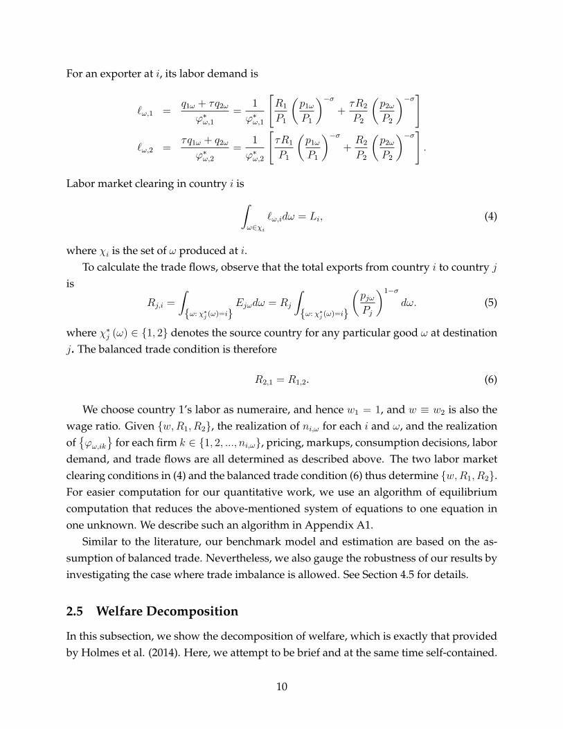
For an exporter at i, its labor demand is

`ω,1 =q1ω + τq2ω

ϕ∗ω,1=

1

ϕ∗ω,1

[R1

P1

(p1ω

P1

)−σ+τR2

P2

(p2ω

P2

)−σ]

`ω,2 =τq1ω + q2ω

ϕ∗ω,2=

1

ϕ∗ω,2

[τR1

P1

(p1ω

P1

)−σ+R2

P2

(p2ω

P2

)−σ].

Labor market clearing in country i is∫ω∈χi

`ω,idω = Li, (4)

where χi is the set of ω produced at i.To calculate the trade flows, observe that the total exports from country i to country j

is

Rj,i =

∫{ω: χ∗j (ω)=i}

Ejωdω = Rj

∫{ω: χ∗j (ω)=i}

(pjωPj

)1−σ

dω. (5)

where χ∗j (ω) ∈ {1, 2} denotes the source country for any particular good ω at destinationj. The balanced trade condition is therefore

R2,1 = R1,2. (6)

We choose country 1’s labor as numeraire, and hence w1 = 1, and w ≡ w2 is also thewage ratio. Given {w,R1, R2}, the realization of ni,ω for each i and ω, and the realizationof{ϕω,ik

}for each firm k ∈ {1, 2, ..., ni,ω}, pricing, markups, consumption decisions, labor

demand, and trade flows are all determined as described above. The two labor marketclearing conditions in (4) and the balanced trade condition (6) thus determine {w,R1, R2}.For easier computation for our quantitative work, we use an algorithm of equilibriumcomputation that reduces the above-mentioned system of equations to one equation inone unknown. We describe such an algorithm in Appendix A1.

Similar to the literature, our benchmark model and estimation are based on the as-sumption of balanced trade. Nevertheless, we also gauge the robustness of our results byinvestigating the case where trade imbalance is allowed. See Section 4.5 for details.

2.5 Welfare Decomposition

In this subsection, we show the decomposition of welfare, which is exactly that providedby Holmes et al. (2014). Here, we attempt to be brief and at the same time self-contained.

10

Let Aj be the price index at j when all goods are priced at marginal cost:

Aj =

∫ ω

0

a∗jω qajωdω,

where qaj={qajω : ω ∈ [0, ω]

}is the expenditure-minimizing consumption bundle that de-

livers one unit of utility. Total welfare is defined as real income Rj/Pj . As the productof producers’ aggregate markup and labor income entails total revenue (3), we can writewelfare at location i as

W Totalj =

Rj

Pj= wjLj ×M sell

j ×1

Pj

= wjLj ×1

Aj×Aj ×M buy

j

Pj×M sell

j

Mbuyj

≡ wjLj ×W Prodj ×WA

j ×W Rj .

Without loss of generality we focus on the welfare of country 1, and by choosing nu-meraire, we can let w1 = 1. As the labor supply Lj is fixed in the analysis, the first termin the welfare decomposition is a constant that we henceforth ignore. The second term1/Aj is the productive efficiency index W Prod

j ; this is what the welfare index would be withconstant markup. The index varies when there is technical change determining the un-derlying levels of productivity. It also varies when trade costs decline, decreasing thecost for foreign firms to deliver goods to the domestic country. Terms-of-trade effects alsoshow up in W Prod

j because a lower wage from a source country raises the index.The third term is the allocative efficiency index WA

j

WAj ≡

Aj ×M buyj

Pj=

∫ ω0a∗jω q

ajωdω∫ ω

0a∗jω qjωdω

≤ 1. (7)

The inequality follows from the fact that under marginal cost pricing, qajω is the optimalbundle, whereas qjω is the optimal bundle under actual pricing. If markups are constant,then for any pair of goods, the ratio of actual prices equals the ratio of marginal cost. Inthis case, the two bundles become the same and WA

j = 1. Once there is any dispersion ofmarkups, welfare deteriorates because resource allocation is distorted. Goods with highermarkups are produced less than optimally (employment is also less than optimal), andthose with low markups are produced more than optimally (employment is also morethan optimal).

The fourth term is a “terms of trade” effect on markups that depends on the ratio

11

of producers’ aggregate markup to consumers’ aggregate markup; thus we call it rela-tive markup effect W R

j . This term is intuitive because a country’s welfare improves whenits firms sell goods with higher markups while its consumers buy goods with lowermarkups. This term drops out in two special cases: under symmetric countries wherethe two countries are mirror images of each other; and under autarky, as there is no dif-ference between the two aggregate markups.

Note that as Holmes et al. focus on the symmetric country case, they do not explicitlyanalyze the relative markup effectW R

j . As fitting to the Chinese economy, we allow asym-metries between countries in all aspects of the model (labor force, productivity distribu-tion, entry and wages). Also note that the above decomposition only requires homotheticpreference and is thus applicable to all market structures.10

2.6 The Productive Efficiency and the ACR Formula

As is well known, the ACR welfare formula captures the gains from trade globally (i.e., forarbitrary changes in trade cost) in a certain class of models with a constant trade elasticity.This class includes BEJK and features no pro-competitive effect. In our model in whichpro-competitive effects may exist and trade elasticity may vary, the ACR formula doesnot hold for arbitrary changes in trade costs. Nevertheless, as pointed out by ACR, formodels with variable trade elasticity, the ACR formula may still capture the total gainsfrom trade locally (i.e., for infinitesimal changes in trade cost).11 Thus, we are interestedin examining whether our model predicts larger/smaller or similar total gains from tradeas compared with the local ACR formula.

We start the comparison by examining the similarity between the productive efficiencyW Prodj and the ACR welfare formula. Note that ACR’s proof of their theorems covers both

perfect competition and monopolistic competition. They do not prove why the BEJKmodel, which features head-to-head Bertrand competition, fits their formula. As Holmeset al. (2014) highlights, the distributional assumption and the number of firms are thekey. Whereas BEJK features a constant trade elasticity, the trade elasticity in our model isa variable, and thus the macro restriction R3 in ACR does not hold here.

Following ACR, the import demand system is a mapping from ({wi}, {τ ij},{Ni}) intoX ≡ {Xij}, where Xij is the trade flow from i to j and Ni is the measure of goods thatis produced in each country i. R3 in ACR is a restriction on partial trade elasticity εii′j ≡

10For welfare decomposition under non-homothetic preference and monopolistic competition, see Wein-berg (2015) and Dhingra and Morrow (2016).

11See footnote 13 and page 109 in ACR. This statement is true if the restriction R3 in their paper holdslocally.

12

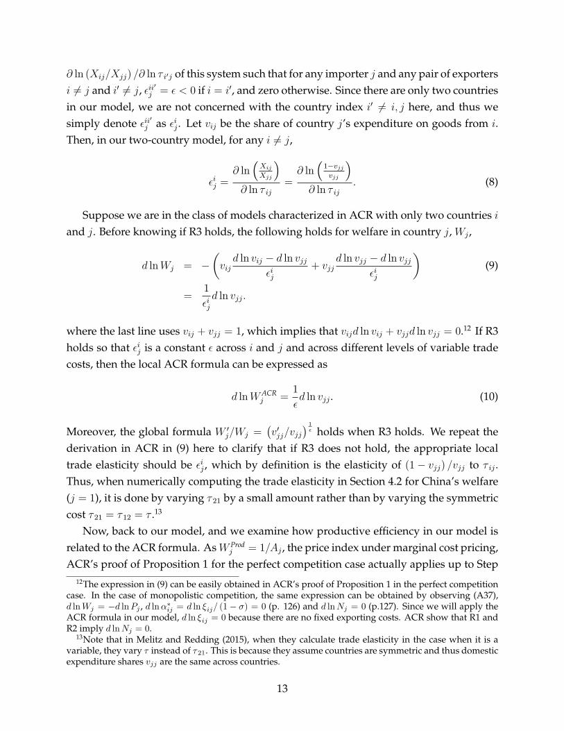
∂ ln (Xij/Xjj) /∂ ln τ i′j of this system such that for any importer j and any pair of exportersi 6= j and i′ 6= j, εii′j = ε < 0 if i = i′, and zero otherwise. Since there are only two countriesin our model, we are not concerned with the country index i′ 6= i, j here, and thus wesimply denote εii′j as εij . Let vij be the share of country j’s expenditure on goods from i.Then, in our two-country model, for any i 6= j,

εij =∂ ln

(XijXjj

)∂ ln τ ij

=∂ ln

(1−vjjvjj

)∂ ln τ ij

. (8)

Suppose we are in the class of models characterized in ACR with only two countries iand j. Before knowing if R3 holds, the following holds for welfare in country j, Wj ,

d lnWj = −(vijd ln vij − d ln vjj

εij+ vjj

d ln vjj − d ln vjjεij

)(9)

=1

εijd ln vjj.

where the last line uses vij + vjj = 1, which implies that vijd ln vij + vjjd ln vjj = 0.12 If R3holds so that εij is a constant ε across i and j and across different levels of variable tradecosts, then the local ACR formula can be expressed as

d lnWACRj =

1

εd ln vjj . (10)

Moreover, the global formula W ′j/Wj =

(v′jj/vjj

) 1ε holds when R3 holds. We repeat the

derivation in ACR in (9) here to clarify that if R3 does not hold, the appropriate localtrade elasticity should be εij , which by definition is the elasticity of (1− vjj) /vjj to τ ij .Thus, when numerically computing the trade elasticity in Section 4.2 for China’s welfare(j = 1), it is done by varying τ 21 by a small amount rather than by varying the symmetriccost τ 21 = τ 12 = τ .13

Now, back to our model, and we examine how productive efficiency in our model isrelated to the ACR formula. AsW Prod

j = 1/Aj , the price index under marginal cost pricing,ACR’s proof of Proposition 1 for the perfect competition case actually applies up to Step

12The expression in (9) can be easily obtained in ACR’s proof of Proposition 1 in the perfect competitioncase. In the case of monopolistic competition, the same expression can be obtained by observing (A37),d lnWj = −d lnPj , d lnα∗ij = d ln ξij/ (1− σ) = 0 (p. 126) and d lnNj = 0 (p.127). Since we will apply theACR formula in our model, d ln ξij = 0 because there are no fixed exporting costs. ACR show that R1 andR2 imply d lnNj = 0.

13Note that in Melitz and Redding (2015), when they calculate trade elasticity in the case when it is avariable, they vary τ instead of τ21. This is because they assume countries are symmetric and thus domesticexpenditure shares vjj are the same across countries.

13

3 with Wj and Pj there replaced with W Prodj and Aj here. That is, letting vij and εij be the

share of country j’s expenditure on goods from i and the trade elasticity under marginalcost pricing, we have

d lnAj =

n∑i=1

vijd ln vij − ln vjj

εij.

Similar to (9), for any i 6= j, the above implies

d lnW Prodj = −d lnAj =

1

εijd ln vjj . (11)

Note that the ACR formula (10) should be applied using actual trade flow to calculatetrade elasticity and domestic expenditure share (that is, actual pricing (2) should be used),whereas (11) uses those under marginal cost pricing. However, there is a special case inwhich vjj = vjj and hence εij = εij . When σ = 1, the preference becomes Cobb-Douglas:

U = exp

(∫ ω

0

ln qωdω

),

and the expenditure share on each good becomes the same (not responsive to prices). Asthe domestic expenditure share is simply the fraction of all goods consumed in countryj that originate in country j, vjj = vjj . By (8), εij = εij . In this case, d lnWACR

j = d lnW Prodj

with the trade elasticity being εij . But, as εij varies with trade shock dτ , where τ = {τ ij},the global ACR formula does not apply.

We have now proved the following proposition. Note in particular that this proposi-tion is applicable to all distributions of productivity draws and of per-product number offirms.

Proposition 1. For infinitesimal changes in τ , the change in the productive efficiency W Prodj can

be expressed as

d lnW Prodj =

1

εijd ln vjj,

where εij and vjj are trade elasticity and domestic expenditure share under marginal cost pricing.When σ = 1 (Cobb-Douglas case), vjj = vjj , εij = εij , and d lnWACR

j = d lnW Prodj .

In the case of σ = 1, this proposition says that for infinitesimal changes in τ , the ACRformula captures productive efficiency but not the total gains from trade. That is, in thiscase,

d lnW Totalj − d lnWACR

j = d lnWA + d lnW Rj .

14

The distributional assumption in BEJK entails d lnWA +d lnW Rj = 0 because the resulting

markup distribution is invariant to trade cost. This is not the case here. Our quantitativeanalysis in Section 4.2 reveals that in the general case of σ > 1, d lnWACR

j is still relativelyclose to d lnW Prod

j ; therefore the total gains d lnW Totalj are larger than d lnWACR

j .For the intuition behind the gap, we distinguish all possible six cases of pricing, markups,

and trade flows in the following table. Without loss of generality, we focus on the marketat country 1, i.e., j = 1. Denote (i, i′) as the pair of locations where the first and secondlowest marginal costs to deliver to country 1 are located. We use (ı) to denote the casewhen the lowest marginal cost is from country i and it charges the monopoly price inequilibrium.

(1, 1) (1, 2) (2, 1) (2, 2) (1) (2)

markup ϕ∗1ϕ∗∗1

τwϕ∗1ϕ∗2

ϕ∗2τwϕ∗1

ϕ∗2ϕ∗∗2

σσ−1

σσ−1

price 1ϕ∗∗1

τwϕ∗2

1ϕ∗1

τwϕ∗∗2

σσ−1

1ϕ∗1

σσ−1

τwϕ∗2

markup affected by τ No Yes Yes No No Noimport affected by τ No No No Yes No Yes

Note that for infinitesimal changes, the effect of a good ω switching between casescan be ignored because at the border between any two cases, the markups must be thesame. Thus, apart from the general equilibrium effect on macro variables, the above tableprovides a comprehensive anatomy of the effect of changes in τ . Thus, apart from thegeneral equilibrium effect onRj and Pj , import is affected by τ directly in the cases whereprices are affected by τ and the suppliers are located at country 2. We ignore the effect onexport because import is what is needed for the ACR formula. To look at pro-competitiveeffects, we look at only two cases where markups are affected by trade cost – (1, 2) and(2, 1). In Case (1, 2), a lower τ decreases both the price and markup but has no effect onimport because the supplier is domestic; this is similar to the entry-deterence examplementioned in the introduction. In Case (2, 1), a lower τ increases the markup but doesnot affect the price and import because the foreign supplier is only constrained by thedomestic best. Thus, in cases where markups are affected by τ , imports are unaffected. Ifthe expenditure share of each case is unaffected by small changes in τ , then the welfareimpacts of τ via markups are totally independent of imports (Proposition 1). The reasonwhy Proposition 1 need not hold under σ > 1 is that changes in trade cost τ may changethe expenditure shares across goods and hence across different cases. Nevertheless, itwill be seen in the quantitative analysis in Section 4.2 that the effects due to changes inexpenditure share are minor, as the extra gains from trade over the ACR formula remainroughly those due to pro-competitive effects.

15

The above table shows how head-to-head competition separates markups and import.In contrast, the total gains from trade in EMX can be captured by the ACR formula be-cause even with finite number of firms, each firm owns a variety and hence a demandcurve along which the pricing is determined, taking into account of strategic interactionsamong firms. A change in τ changes the foreign supplier’s delivered marginal cost, andtherefore changes the price, markup, and import simultaneously. Similarly, even thoughthe ACR formula must be modified in Arkolakis et al. (2017) to account for the changefrom CES preference to a general preference that allows variable markup, the fact thateach firm owns a variety under monopolistic competition still makes trade flows suffi-cient statistics for welfare gains from trade.

3 Quantifying the Model

We use the following two steps to quantify the model. First, we estimate the markupdistribution and infer the elasticity of substitution from such distribution. Then, given σ,measures of {w,R1, R2}, we use the moments of markups, trade flows, number of firmsand fraction of exporters to estimate the remaining parameters by SMM. Note that unlikeEMX whose benchmark focuses on symmetric countries, our empirical implementationfocuses on asymmetric countries, as the large wage gap between China and the ROWshould not be ignored since it may have a large impact on parameter estimates, as wellas potential large general equilibrium effects in counter-factuals. Despite the lack of firm-level data in the ROW, we demonstrate that separating moments of exporters and non-exporters can help identify the different parameters of the two countries.

3.1 Data

Our firm-level data set comes from the Economic Census data (1995 and 2004) fromChina’s National Bureau of Statistics (NBS), which covers all manufacturing firms, in-cluding SOEs. The sample sizes for 1995 and 2004 are 458, 327 and 1, 324, 752, respec-tively.14 The advantage of using this data set, instead of the commonly used firm-levelsurvey data set, which reports all SOEs and only those private firms with revenues of atleast 5 million renminbi, is that we do not have to deal with the issue of truncation. Aswe are concerned with potential resource misallocation between firms, it is important to

14The original data sets have larger sample sizes, but they also include some (but not all) non-manufacturing industries, as well as firms without independent accounting and village firms, which en-tail numerous missing values. The final sample is obtained after excluding these cases and adjusting forindustrial code consistency.

16

have the entire distribution. We estimate the models separately for the years 1995 and2004.

We obtain world manufacturing GDP and GDP per capita from the World Bank’sWorld Development Indicators (WDI). The aggregate Chinese trade data is obtained fromthe UN COMTRADE.

3.2 Estimation of Markups

Under constant returns to scale assumption, a natural way to estimate markups is bytaking the ratio of revenue to total costs, i.e., revenue productivity, or what we call rawmarkup. However, it is important to recognize that, in general, raw markups may differacross firms, not only because of the real markup differences, but also because of differ-ences in the technology with which they operate. To control for this potential source ofheterogeneity, we use modern IO methods to purge our markup estimates of the differ-ences in technology. In particular, we estimate markups following DLW’s approach,15

who calculate markups as

mω =θXωαXω

,

where θXω is the input elasticity of output for input X , and αXω is the share of expenditureon input X in total revenue. To map our model into firm-level data, we relax the assump-tions of a single factor of production and constant returns to scale. Following DLW, weassume a translog production function.16 The estimation of firm-level markup hinges onchoosing an input X that is free of any adjustment costs, and the estimation of its outputelasticity θXω . As labor is largely not freely chosen in China (particularly SOEs) and capitalis often considered a dynamic input (which makes its output elasticity difficult to inter-pret), we choose intermediate materials as the input to estimate firm markup (see alsoDLW). The full details of the markup estimation are relegated to Appendix A2.

Table 1 gives summary statistics of the markup distribution,17 with breakdowns ineach year and between exporters and non-exporters. Observe that the (unweighted)

15We also conduct estimation and counter-factual analysis under raw markups as a robustness check.16In our implementation of the DLW approach using Chinese firm-level data under the translog produc-

tion function, which allows variable returns to scale, it turns out that the returns to scale are quite closeto constant. See Table A1 in the appendix. Interestingly, EMX also found similar results using Taiwanesefirm-level data.

17Following the literature, e.g., Goldberg, De Loecker, Khandelwal and Pavcnik (2015) and Lu and Yu(2015), we trim the estimated markup distribution in the top and bottom 2.5 percentiles to alleviate theconcern that the extreme outliers may drive the results. Our results are robust to alternative trims (e.g, thetop and bottom 1%; results are available upon request). We also drop estimated markups that are lowerthan one, as our structural model does not generate such markups.

17

mean markups all decrease between 1995 and 2004 for all firms, both exporters and non-exporters. The (unweighted) standard deviation of markups decreases for non-exporters,but increases slightly for exporters. Because there are more non-exporters than exportersand the decrease in non-exporters’ standard deviation is larger than the increase in ex-porter’s standard deviation, the overall standard deviation decreases. Almost all of thepercentiles decreased between 1995 and 2004. This is consistent with the pattern seen inFigure 1 where the entire distribution becomes more condensed.

However, we note that the pattern described in Table 1 only hints at the existence ofpro-competitive effects. The reduction of dispersion of firm markups does not necessar-ily mean that the allocative efficiency increases because allocative efficiency depends onconsumers’ markups rather than firms’ markups. It does show that the markets facingChinese firms became more competitive. Also, we cannot reach a conclusion yet aboutthe relative markup effect, as we do not observe the consumers’ aggregate markup di-rectly. We need to quantify the model and simulate both types of markups to conductwelfare analysis.

3.3 Elasticity of Substitution

As a preference parameter, we infer a common elasticity of substitution σ for both years.Note that the model implies thatm ∈

[1, σ

σ−1

], and hence the monopoly markup is the up-

per bound of markup distribution. Recall the economics behind this. An active firm of aproduct charges the second lowest marginal cost when such cost is sufficiently low. Whenthe second marginal cost is high, the markup is bounded by the monopoly markup be-cause the firm’s profit is still subject to the substitutability between products. The higherthe substitutability (σ), the lower the monopoly markup the firm will charge.

As we examine the effects of markups, we infer σ using the upper bound of themarkup distribution. Considering the possibility of measurement errors and outliers,we equate σ/ (σ − 1) to the 99th percentile of the estimated markup distribution (usingthe pooled sample from 1995–2004). We obtain σ = 1.40, which reflects that the 99th per-centile is around 3.5.18 This calibrated σ = 1.40 is strikingly similar to the estimate ofthe same parameter (1.37) in Simonovska and Waugh (2014b) with the optimal weightingmatrix in their method of moments procedure.

The inferred σ here is quite different from those estimates in models that feature con-stant markups (often a CES preference coupled with either monopolistic competition or

18Note that this estimate of σ is not sensitive to sample size. In our multi-sector exercise, σs is separatelyinferred for each sector s using the markup distribution of that sector. The unweighted mean of σs is 1.44,and 23 out of 29 σs are within one standard deviation from the mean, (1.27, 1.61). See Section 5.1.

18

perfect competition). This is essentially because σ/ (σ − 1) in our model is the upperbound rather than the average of markups. Under a constant-markup model and usingthe harmonic mean of firm markups in 1995, 1.259, this implies σ = 4.86. However, inthe current model, this value of σ implies that m ∈ [1, 1.259], which cuts 50.6% off theestimated markup distribution. Then, these large markups where most distortions comefrom are ignored. In fact, the pro-competitive effects of trade become negligible underm ∈ [1, 1.259] because the associated allocative efficiency is much closer to the first-bestcase (constant markup) without the very skewed larger half of the markups. EMX alsofound that the extent of pro-competitive effects depends largely on the extent to whichmarkups can vary in the model.

Note that in BEJK, the trade elasticity is given the tail index of the Frechét distribution,and is independent of the elasticity of substitution σ. In our model where the productivitydraws deviate from Frechét, σ may potentially matter in determining trade elasticity, butthe effect seems small, as we will see in Section 4.2 that the trade elasticities in our modelare quite close to those found by Simonovska and Waugh (2014b) under the BEJK model.

3.4 Simulated Method of Moments

3.4.1 Method

We estimate the remaining parameters using SMM for 1995 and 2004 separately. It isimportant to allow all parameters to vary between the two years so that the changes inthe environment of the Chinese economy can be reflected. If we instead have the changein trade cost τ in between two years explain all the changes in the observed moments,then the role of trade cost may be exaggerated.

For i = 1, 2, the remaining parameters are

τ : trade costγ : total measure of goodsλi : mean number of entrants per productµi : mean parameter of log-normal productivity drawηi : standard deviation parameter of log-normal productivity draw

Note that for productivity, we normalize µ2 = 0 (when lnϕ is zero, ϕ = 1) becauseonly the relative magnitude of µ1 to µ2 matters. Choosing µ2 amounts to choosing a unit.In order to use SMM to estimate these seven parameters, we need at least seven mo-ments. We use the following 12 moments: the import and export shares; relative numberof firms; fraction of exporters; weighted mean and standard deviation of cost shares for

19

both exporters and non-exporters; and the median and 95th percentile of cost shares forexporters and non-exporters.19

Recall that the actual measure of goods is given by (1): ω = γ[1− e−(λ1+λ2)

], but this

is not directly observed. What is observable is the number of active Chinese firms:

N1 = γ(1− e−λ1

)× Pr

[1

ϕ∗1ω<wτ

ϕ∗2ω

].

Divide both sides by N , a large number that is chosen for normalization. The moment weuse is the relative number of Chinese firms:

N1

N=γ(1− e−λ1

)N

× Pr

[1

ϕ∗1ω<wτ

ϕ∗2ω

], (12)

The choice of N does not affect the estimates, but we must choose the same N for both1995 and 2004 in order to gauge the increase in γ. For this purpose, we choose N to be 2

million.20

As our data shows whether a firm is an exporter or not, we use moments of exportersand non-exporters separately because the way in which parameters of countries 1 and 2(China and the ROW) enter these moments differs between these two groups. The intu-ition is clear: Chinese exporters face direct competition in the ROW’s markets and non-exporters face foreign competition on their home turf. As we lack firm-level data from theROW, this approach is crucial for backing out the parameters of the ROW.21 The parame-ters of the ROW is not needed in a symmetric-country estimation/calibration, which mayexplain why it is often adopted in the literature. We will also estimate a symmetric coun-try version for comparison. Nevertheless, our exercise demonstrates that this approach ofseparating moments of exporters and non-exporters works well for asymmetric-countryestimation.

Note that our model structure implies that all of the above-mentioned moments canbe simulated for a given set of parameters and observed macro variables {w,R1, R2}.Thus, our SMM procedure essentially searches for the set of parameters that are mostconsistent with the observed micro moments given observed macro variables {w,R1, R2}.

19The import share is the import penetration ratio, i.e. IM/(R1-EX+IM), and the export share is the totalexport divided by the same denominator. All the cost share moments are weighted by revenues.

20Recall that we have 1, 324, 752 firms in our 2004 data. Also, larger N generates a larger number of goods(and hence draws from both distributions in the model) in simulation, and the law of large numbers helpsto generate more precise moments.

21Whereas using such firm-level data with information on firms’ exporting status gives the advantageof backing out parameters for the ROW, it also implies that one cannot use a n-country model with n ≥ 2unless one can gather firm-level data for all of these countries, which is a daunting task.

20

One advantage of this approach is that we do not have to measure or estimate the difficultobject country sizes {L1, L2} as this may well depend on human capital in addition topopulation sizes and other things.22 After we obtain parameter estimates, we simulatethe model given observed macro variables {w,R1, R2} to impute {L1, L2} by simulatingthe labor demand across all goods and using the labor-market clearing conditions. Then,our counter-factual is based on the parameter estimates and the imputed {L1, L2}, and ofcourse the macro variables {w,R1, R2} are endogenous in counter-factuals.

How the macro variables {w,R1, R2} are obtained from data is as follows. To calculatew = w2/w1, we first obtain the GDP per capita of China and the ROW from WDI.23 Wethen calculate wi by multiplying GDP per capita by the labor income shares for the ROWand China, which are taken from Karabarbounis and Neiman (2014).24 For R1 and R2, wefirst obtain the manufacturing GDPs of China and the ROW from WDI data. We then usethe input-output table for China (2002) and the US (1997–2005) to obtain GDP’s share oftotal revenue. We then use such shares and the manufacturing GDPs to imputeR1 andR2

as total revenue. Although our model does not distinguish value added and revenue, wechoose to interpret Ri as total revenue rather than GDP to be consistent with our exportand import moments, which are also in terms of revenue.

3.4.2 SMM Result

The estimation result is shown in Table 2. The model fits the data moments reasonablywell, and the small standard errors indicate that each parameter is relatively preciselyestimated. For each year (1995 or 2004), we impute {L1, L2} given the parameter esti-mates and observed macro variables {w,R1, R2}. Then, under parameter estimates andthe imputed {L1, L2}, we simulate {w,R1, R2}. Note that the simulated {w,R1, R2} andthe observed ones need not be the same. Nevertheless, the bottom three rows in Table 2show that they turn out to be quite close,25 serving as additional validation of the model.

As we estimate the models for 1995 and 2004 separately, the changes of the parametersare strikingly consistent with well-known empirical patterns about the Chinese economyduring this period. From 1995 to 2004, the estimate of τ shows a dramatic decrease from2.31 to 1.66. The measure of goods γ more than triples from 0.26 to 0.85. This basically re-

22Moreover, it is also difficult to find a robust way to combine the population size and human capitalacross different countries in the rest of the world.

23The ROW’s GDP per capita is the population-weighted average of GDP per capita across all countriesother than China.

24The ROW’s labor share is the weighted average of labor share across all countries besides China, withthe weight being relative GDP.

25Here, the largest discrepancy between data values and simulated value is the total revenue of the ROWin 1995, which is about 10.5%. For all the other numbers, the discrepancies are all less than 5.2%.

21

flects the sharp increase in the number of firms between the two Economic Censuses, from458,327 in 1995 to 1,324,752 in 2004, which is almost triple. The mean number of entrantsper product in China (λ1) increased from 2.44 to 2.61, whereas in the ROW it increasedfrom 5.29 to 5.83. China’s mean log productivity (µ1) relative to the ROW increased from−2.40 to −1.79. These numbers are negative, meaning that China’s productivity is lowerthan that of the ROW (µ2 is normalized to 0). Also, we see a slight decrease in the dis-persion parameter of the productivity distribution in both countries (η1, η2). Interestingly,the productivity dispersion is larger in China than in the ROW, which is consistent withthe finding by Hsieh and Klenow (2009).26

Based on the 2004 estimation, we calculate a Jacobian matrix in which each entry givesa rate of change of a moment to a parameter, and this is shown in Table 3. The larger theabsolute value of a rate of change, the more sensitive this moment is to the parameter,and hence the more useful this moment is in identifying this parameter, at least at thelocal area of the optimal estimates. With such Jacobian matrices, the asymptotic variance-covariance matrices of the optimal estimates can be calculated to produce the standarderrors reported in Table 2.

Trade cost τ affects almost all moments significantly, and it is natural to see that thetwo trade moments, the relative number of Chinese firms and the fraction of exportersare particularly strong for identifying this. Interestingly, when τ increases, the 95th per-centiles of markups for both exporters and non-exporters increase sharply. For non-exporters, this is intuitive because a higher τ provides non-exporters more insulationfrom foreign competition, and the top non-exporters gain more from this. For exporters,a higher τ makes it harder for them to compete in foreign markets, but recall that an ex-porter’s markup is a harmonic mean of the markups in both the domestic and foreignmarkets. It must be that the gains in markups at home outweigh the losses in markups inforeign markets.

For λ1 and λ2, the 95th percentiles of markups and the relative number of active firmsare crucial in identifying these two parameters, with the trade moments playing some roleas well. The intuition is as follows. Fixing other parameters, when λi increases, the num-ber of entrants per product in country i increases. Due to the non-fat-tailed nature of theproductivity distribution, the ratio between the top two draws is narrowed, but since this

26The mean of a log-normal distribution is eµ+η2/2. According to our estimates of µ1 and η1 in these two

years, this translates to an annual productivity growth rate of 6.9%. This impressive growth rate is actuallysimilar to the 7.96% estimated by Brandt, Van Biesebroeck and Zhang (2012). Note that the 6.9% growthrate here is relative to the ROW. If the ROW also grows in their productivity, the actual productivity growthrate could be even higher. In fact, Brandt, Van Biesebroeck, Wang, and Zhang (2012) find a 12% average TFPgrowth rate at industry level. The data used in both above-mentioned papers is the annual manufacturingsurvey data from 1998 to 2007.

22

ratio is indeed the markup and since this is particularly pronounced for the top markups,the 95th percentiles are particularly useful in identifying these two parameters. The factthat we observe increases in λi during this period may reflect that the 95th percentiles ofmarkups decrease during this period. Intuitively, the relative number of (active) Chinesefirms is also useful for identifying λ1, as seen clearly in (12).27

For the measure of goods γ, it is obvious that the relative number of Chinese firmsis the most useful moment. An increase in mean productivity parameter µ1 increasesexport share, the number of Chinese firms, and the fraction of exporters, but decreases theimport share. These are all intuitive. However, an increase in µ1 sharply increases the 95thpercentile markup for non-exporters but sharply decreases the 95th percentile markup forexporters. This is because top non-exporters are actually not the most productive firms– their productivities are somewhere in the middle of the distribution and hence theygain in markup by having higher productivity. In contrast, top exporters are the mostproductive firms, and they lose in markup when they become even more productive, dueto the compression at the upper tail of the productivity distribution.

For η1 and η2, first note that they are not only dispersion parameters, but their in-creases induce increases in means as well. Hence, the direction of changes due to a changein η1 is similar to that of a change in µ1, but the intensities are quite different. For example,η1 has much larger effects on moments of markups, including both means and standarddeviations of the cost shares, than µ1. Moreover, the 95th percentile markup for exportersis extremely sensitive to η1 because η1 affects the top productivities much more than µ1.Also note the interesting pattern: η1 and η2 almost always affect moments in oppositeways. An increase in η2 increases both the mean and dispersion of the ROW’s productiv-ity, and this increases China’s import share, and decreases China’s export share, numberof firms and fraction of exporters. It decreases Chinese non-exporters’ median and 95thpercentile markups, but increases those of Chinese exporters.

Finally, we discuss a point that is often mentioned in studies of the Chinese econ-omy. China underwent various reforms, including but not limited to trade reforms, inthis decade. One notable reform is that of SOEs during the late 90s, which is well knownto have made China’s various industries more competitive. Although we do not modelthe source of distortion explicitly in our model and rather treat markups (and their dis-tribution) as a reflection of distortion, the fact that we observe increases in both λ1 and γ

may be partly due to these reforms. The compression in markup distribution (Table 1 and

27Trade flows are also useful, as an increase in λ1 raises active firms’ productivities in China, increasingthe export share and reducing the import share. On the other hand, an increase in λ2 raises active firms’productivities in the ROW, increasing the import share and reducing the export share in China.

23

Figure 1) and the increasing number of manufacturing firms are also consistent with theabove-mentioned reforms.

4 Gains from Trade

In this section, we conduct a battery of counter-factual analyses to examine the welfaregains from trade.

4.1 Welfare Analysis: Between 1995 and 2004 and from Autarky

To examine gains from trade, we conduct two counter-factual analyses by fixing all pa-rameter values at the 2004 level and changing only τ . In the first analysis, we simulatewelfare and its components when τ is changed to the 1995 level, and we calculate thepercentage changes of welfare and its components. In the second analysis, we take τ toan inhibitive value so that the economy becomes autarky.

The results are shown in Table 4. The welfare gains of changing τ from 1995’s level to2004’s level are 9.4%, in which allocative efficiency accounts for 22.3% (2.1/9.4) and rela-tive markup effect accounts for 3.1% (0.3/9.4). Thus, these pro-competitive effects jointlyaccount for 25.4% of the total gains from trade. In fact, both aggregate markups M sell andMbuy decrease during this period, which is a natural result under trade liberalization, butthe percentage decrease in the consumers’ aggregate markup Mbuy is larger. Overall, al-though the relative markup effect is positive, it is relatively small, whereas the combinedeffect can account for about a quarter of the total gains. The total gains from autarky to2004’s τ are, of course, much larger, at 33.4%, but the decomposition is similar to the firstanalysis.

For the intuition regarding the source of the gains due to allocative efficiency, recallthe six cases of markups facing Chinese consumers distinguished in Section 2.6. A changein trade cost affects markups only in cases (1, 2) and (2, 1). Trade liberalization depressesmarkups in case (1, 2), but increases markups in case (2, 1). Because foreign firms typ-ically face fiercer competition due to the trade barrier, case (1, 2) has on average highermarkups relative to case (2, 1); thus trade liberalization reduces markup dispersion andenhances allocative efficiency.

Next, we examine whether the result of “diminishing returns in openness” in EMXholds here. The following table summarizes the welfare gains reported in their study,as well as the breakdown in Ricardian gains and allocative efficiency. There is an obvi-ous “diminishing returns” in allocative efficiency, as the opening up from autarky to 10%

24

import share improves welfare by 1.2%, whereas further opening up from 10% to 20% im-proves welfare by only 0.3%. But such a diminishing-returns pattern does not show up inthe Ricardian component. As a result, the contribution of allocative efficiency diminishesrapidly from 1.2/3.1 ≈ 38% to 0.3/2.8 ≈ 10.7%.

Import share %∆ in EMX Importance of WA

Total Welfare Ricardian WA

0 to 10% 3.1 1.9 1.2 38.7%

10% to 20% 2.8 2.5 0.3 10.7%

Panel B of Table 4 reports the result from a similar exercise. Note that EMX’s pro-competitive effect only includes allocative efficiency but not the relative markup effectas their formulation focuses on symmetric countries. To compare, we ignore the relativemarkup effect. A similar diminishing returns pattern in allocative efficiency is obvious,dropping from 5.5% to 1.5%. But, unlike in EMX, we also see sharp diminishing returnsin our counter-factuals for total welfare and the Ricardian component. As a result, we donot see a diminishing contribution in allocative efficiency. Indeed, the contribution staysaround 24%, which is quite close to the results reported in Panel A.

Looking at both panels together, the contribution of pro-competitive effects range from23.3% to 27.6%, and the contribution of allocative efficiency ranges from 22.3% to 24.6%.Despite the differences in model structures, our estimates turn out to be in the ballpark ofEMX’s estimates, which range from 11% to 38%.

4.2 Comparison with the ACR Formula

In this subsection, we compare the welfare gains in this model with the ACR formulain two ways. First, we compare with the local ACR formula for small changes in tradecost. Second, as trade elasticity is a variable, we integrate the local formula to examinethe gains from 1995’s τ to 2004’s τ in a similar fashion to Panel A of Table 4.

For the first comparison, recall from Section 2.6 that for the case of σ = 1 (Cobb-Douglas), the ACR formula captures the gains in productive efficiency for small changesin trade costs, but not the total gains from trade. For general σ > 1, analytical results onthe comparison with the ACR formula are not available, and here we provide a quantita-tive analysis based on the estimated models at 1995 and 2004. For this exercise, we investi-gate the effect of a small reduction h in the logarithm of trade cost so that ln τ ′ = ln (τ)−h.The results are reported in Table 5. Here, the welfare gains are expressed in terms of elas-ticity to trade cost, i.e., d ln (W ) /d ln τ , where W can be W Total,W Prod,WA×WR, or WACR.

25

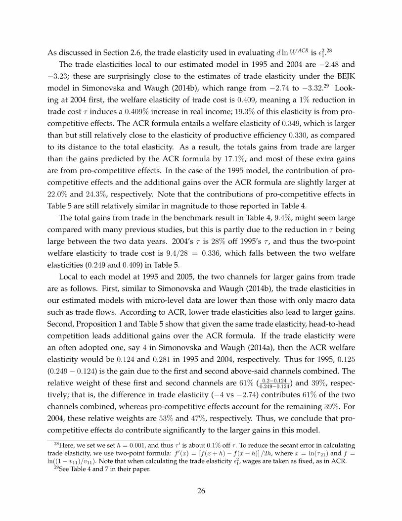
As discussed in Section 2.6, the trade elasticity used in evaluating d lnWACR is ε21.28

The trade elasticities local to our estimated model in 1995 and 2004 are −2.48 and−3.23; these are surprisingly close to the estimates of trade elasticity under the BEJKmodel in Simonovska and Waugh (2014b), which range from −2.74 to −3.32.29 Look-ing at 2004 first, the welfare elasticity of trade cost is 0.409, meaning a 1% reduction intrade cost τ induces a 0.409% increase in real income; 19.3% of this elasticity is from pro-competitive effects. The ACR formula entails a welfare elasticity of 0.349, which is largerthan but still relatively close to the elasticity of productive efficiency 0.330, as comparedto its distance to the total elasticity. As a result, the totals gains from trade are largerthan the gains predicted by the ACR formula by 17.1%, and most of these extra gainsare from pro-competitive effects. In the case of the 1995 model, the contribution of pro-competitive effects and the additional gains over the ACR formula are slightly larger at22.0% and 24.3%, respectively. Note that the contributions of pro-competitive effects inTable 5 are still relatively similar in magnitude to those reported in Table 4.

The total gains from trade in the benchmark result in Table 4, 9.4%, might seem largecompared with many previous studies, but this is partly due to the reduction in τ beinglarge between the two data years. 2004’s τ is 28% off 1995’s τ , and thus the two-pointwelfare elasticity to trade cost is 9.4/28 = 0.336, which falls between the two welfareelasticities (0.249 and 0.409) in Table 5.

Local to each model at 1995 and 2005, the two channels for larger gains from tradeare as follows. First, similar to Simonovska and Waugh (2014b), the trade elasticities inour estimated models with micro-level data are lower than those with only macro datasuch as trade flows. According to ACR, lower trade elasticities also lead to larger gains.Second, Proposition 1 and Table 5 show that given the same trade elasticity, head-to-headcompetition leads additional gains over the ACR formula. If the trade elasticity werean often adopted one, say 4 in Simonovska and Waugh (2014a), then the ACR welfareelasticity would be 0.124 and 0.281 in 1995 and 2004, respectively. Thus for 1995, 0.125

(0.249− 0.124) is the gain due to the first and second above-said channels combined. Therelative weight of these first and second channels are 61% ( 0.2−0.124

0.249−0.124) and 39%, respec-

tively; that is, the difference in trade elasticity (−4 vs −2.74) contributes 61% of the twochannels combined, whereas pro-competitive effects account for the remaining 39%. For2004, these relative weights are 53% and 47%, respectively. Thus, we conclude that pro-competitive effects do contribute significantly to the larger gains in this model.

28Here, we set we set h = 0.001, and thus τ ′ is about 0.1% off τ . To reduce the secant error in calculatingtrade elasticity, we use two-point formula: f ′(x) = [f(x+ h)− f(x− h)] /2h, where x = ln(τ21) and f =ln((1− v11)/v11). Note that when calculating the trade elasticity ε21, wages are taken as fixed, as in ACR.

29See Table 4 and 7 in their paper.

26

For the second comparison, we integrate the local ACR formula to compute what theirformula would predict for a change in trade cost between 1995 and 2004’s levels. Werelegate the calculation details to Appendix A3. The result is that the gains from tradeaccording to the ACR formula are 7.4%. As the total gains from trade 9.4% (Table 4),they are 27.0% higher than the ACR formula. If the trade elasticity were a constant at −4,then the ACR formula predicts a welfare gain of 5.3%.30 Thus, the first channel (due todifference in trade elasticity) accounts for 51.2% (7.4−5.3

9.4−5.3) of the additional gains, whereas

the second channel (due to head-to-head competition) accounts for the remaining 48.8%.These numbers are similar to those found in the first comparison.

4.3 Symmetric Countries

For the purposes of investigating the role played by the asymmetry between China andthe rest of the world, especially in terms of the differences in relative wage and productiv-ity, we also estimate a symmetric-country case. The assumption of symmetric-countriesis often made in the literature because it allows greater tractability and less data require-ment. Nevertheless, ignoring cross-country differences may miss important gains fromtrade. We demonstrate this point here.

The estimation results are shown in Table 6 and the counter-factual results in Table 7.The changes in trade cost τ , measure of goods γ and number of entrants per product λbetween 1995 and 2004 are all in the same direction as in the benchmark case. Note thatthe estimated λ is similar to a weighted average of estimated λ1 and λ2, with the ROWweighted more heavily, since the ROW is much larger than China. Also, observe thatalthough the standard errors here are somewhat smaller than those in the benchmark es-timation, the fit of moments becomes significantly worse. This is because there are fewerparameters in the symmetric-country estimation, reflecting the fact that the symmetric-country estimation obscures the large discrepancy in entry and productivity distributionseen in Table 2. It may also be partly because the symmetric-country model misses out thegeneral equilibrium effect in the adjustment of relative wages, which change from 10.5 to5.3 (See Table 2), meaning that Chinese wages relative to the ROW almost double in thisdecade.

For counter-factual results, first note that the relative markup effect does not show upin Table 7 because this term drops out under symmetric countries. Note that the overallwelfare gains become much smaller than the benchmark case (e.g. 2.7% versus 9.4%).

30Under the 2004 parameters, domestic consumption share drops from 0.9065 to 0.7368 when trade costτ falls from the 1995 level to the 2004 level.

27

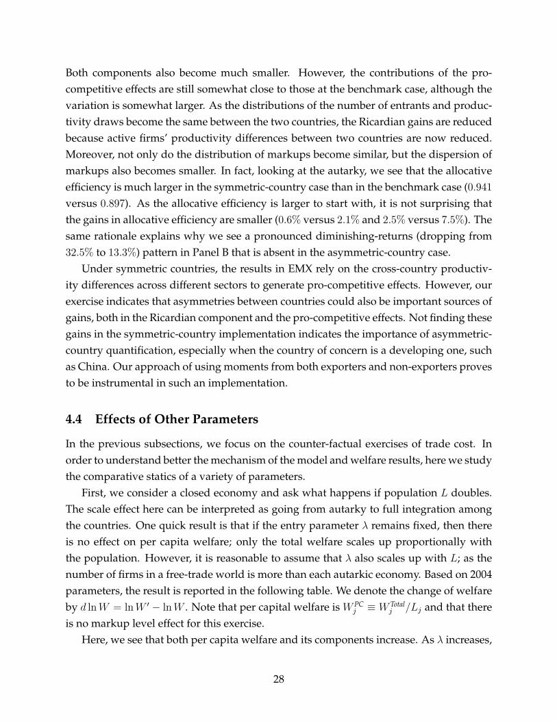
Both components also become much smaller. However, the contributions of the pro-competitive effects are still somewhat close to those at the benchmark case, although thevariation is somewhat larger. As the distributions of the number of entrants and produc-tivity draws become the same between the two countries, the Ricardian gains are reducedbecause active firms’ productivity differences between two countries are now reduced.Moreover, not only do the distribution of markups become similar, but the dispersion ofmarkups also becomes smaller. In fact, looking at the autarky, we see that the allocativeefficiency is much larger in the symmetric-country case than in the benchmark case (0.941

versus 0.897). As the allocative efficiency is larger to start with, it is not surprising thatthe gains in allocative efficiency are smaller (0.6% versus 2.1% and 2.5% versus 7.5%). Thesame rationale explains why we see a pronounced diminishing-returns (dropping from32.5% to 13.3%) pattern in Panel B that is absent in the asymmetric-country case.

Under symmetric countries, the results in EMX rely on the cross-country productiv-ity differences across different sectors to generate pro-competitive effects. However, ourexercise indicates that asymmetries between countries could also be important sources ofgains, both in the Ricardian component and the pro-competitive effects. Not finding thesegains in the symmetric-country implementation indicates the importance of asymmetric-country quantification, especially when the country of concern is a developing one, suchas China. Our approach of using moments from both exporters and non-exporters provesto be instrumental in such an implementation.

4.4 Effects of Other Parameters

In the previous subsections, we focus on the counter-factual exercises of trade cost. Inorder to understand better the mechanism of the model and welfare results, here we studythe comparative statics of a variety of parameters.

First, we consider a closed economy and ask what happens if population L doubles.The scale effect here can be interpreted as going from autarky to full integration amongthe countries. One quick result is that if the entry parameter λ remains fixed, then thereis no effect on per capita welfare; only the total welfare scales up proportionally withthe population. However, it is reasonable to assume that λ also scales up with L; as thenumber of firms in a free-trade world is more than each autarkic economy. Based on 2004parameters, the result is reported in the following table. We denote the change of welfareby d lnW = lnW ′ − lnW . Note that per capital welfare is W PC

j ≡ W Totalj /Lj and that there

is no markup level effect for this exercise.Here, we see that both per capita welfare and its components increase. As λ increases,

28

there are more draws from the productivity distribution. Hence, there are gains due toincreased productivity because “the best” now becomes better. There are also gains inallocative efficiency because of the compression of the ratio between the top two pro-ductivities when there are more draws from a non-fat-tailed distribution.31 The gains inallocative efficiency here are relatively modest compared with the gains due to enhancedproductivity.

L and λ doubles η doubles

d lnW PC1 0.41 0.32

d lnW Prod1 0.35 0.35

d lnWA1 0.06 −0.03

In the case where the standard deviation of log-productivity doubles, both per capitawelfare and productivity efficiency increase, but the allocative efficiency decreases. Theincrease in productive efficiency is readily comprehensible. As η increases, not only doesit increase the mean, but the top productivity is increased even more as the dispersion atthe right-tail increases. In contrast, the increase in the dispersion at the right-tail enlargesthe ratio between the top two productivities, and thus increases markup dispersion andreduces allocative efficiency. However, the effect on productive efficiency dominates andthus per capita welfare still increases.

Next, we return to open economy, and consider symmetric countries for clarity. Wehave seen the effect of trade liberalization in symmetric-country case in the previous sub-section. Here, we want to investigate the role of productivity dispersion (η) and the meannumber of draws (λ, which reflects market structure) on gains from trade. As such, wereplicate the exercise of gains from trade between 1995 and 2004, but under different lev-els of η (Panel A of Table 8), as well as under different levels of λ (Panel B of Table 8).

The middle columns of both panels are the same as that reported in the panel A ofTable 7. Panel A shows that the larger the dispersion of the productivity distribution, thelarger the gains from trade in total and in productive efficiency. When the productivitydraws are more dispersed and hence more skewed to the right, the best productivity ineach country is therefore higher, increasing the gains from trade via productive efficiency.There are always positive gains from trade via improved allocative efficiency, but themagnitude is relatively stable. Thus, the contribution of allocative efficiency diminishesfrom as large as 60% at 0.5 times η0, the standard deviation at 2004, to as small as 14% at1.5 times η0.

31Holmes et al. (2014) highlight this result.

29

In Panel B, gains from trade in total and the two components are all decreasing inthe level of λ. With a given distribution of productivity draws, the more draws suggestthat the top productivity and the ratio between the top two are both operating at a righterpart of the tail. The fact that the log-normal distribution is not fat-tailed implies that tradeliberalization induces smaller increases in the productivities of actual suppliers when λ ishigher, because they were already quite high before trade liberalization. Also, when λ ishigher, the same non-fat-tailed nature implies that trade liberalization induces a smallerreduction in the ratio of the top two productivities because they were already small beforetrade liberalization. The diminishing speed of these two components in λ are roughlythe same, resulting in a relatively stable contribution of pro-competitive effects acrossdifferent λ’s.

4.5 Robustness

We conduct four robustness checks. Recall that in the benchmark case, the counter-factualanalyses are based on 2004 estimates and change τ back to the 1995 level. In our firstrobustness check, we conduct a counter-factual analysis based on 1995 estimates andchange τ to the 2004 level. In our second check, we use an alternative measure of markupsto estimate the model and run counter-factuals. That is, by invoking the constant-returns-to-scale assumption, we calculate raw markups by taking the ratio of revenue to total costs.For our third check, recall that we used the 99th percentile of the markup distribution toinfer σ, but now we also report results based on the 97.5th percentile. In our fourth check,we return to the benchmark but allow for trade imbalance in the model.

The results are reported in Table 9. We omit the numbers of the level of total welfareand its components, and simply report the corresponding percentage changes. The totalgains from trade between 1995 and 2004 range between 5.8% and 7.7%, and the contribu-tion of pro-competitive effects ranges from 19.4% to 27.3%, and that of allocative efficiencyranges from 19.0% to 22.4%. These indicate that the importance of pro-competitive effectsremains similar, and the allocative efficiency still accounts for the bulk of gains from tradeexcept the case with trade imbalance.

The only difference between the first robustness check and the benchmark is that allparameters besides τ are fixed at the 1995 levels instead of at the 2004 levels. Both theoverall gains and the pro-competitive effects are smaller in the first robustness check thanin the benchmark. As China had smaller productivity and smaller entry in 1995, thisindicates a complementary effect between trade liberalization and other fundamentals inthe sense that there are more gains from trade when productivity and entry are higher.

30

Next, note that the σ inferred from raw markups is about 1.67, which implies a smallerupper bound of markups and hence a smaller markup dispersion than the benchmarkcase. So it is not surprising that the pro-competitive effects are slightly less importantunder raw markups. This also explains why using the 97.5th percentile of the markupdistribution to infer σ also induces smaller pro-competitive effects.

There were substantial trade surpluses in China in both 1995 and 2004. They accountfor 2.25% of China’s manufacturing sales in 1995 and 2.63% in 2004. To accommodatetrade imbalance, we follow the literature by allowing an exogenous trade deficit Di foreach country i with the requirement that D1 + D2 = 0.32 With trade deficits, the totalincome in country i is Ri + Di. As China has a trade surplus in both years, we can sethere D2 = D > 0 and D1 = −D, where D is the size of surplus in China. The detailsabout the equilibrium conditions, the algorithm, and the implementation of SMM of thismodified model can be found in Appendix A4. The contribution from pro-competitiveeffects remain similar to the benchmark results in Table 4. Even though the contributionfrom allocative efficiency remain sizable at 19%, the relative markup effect accounts for8.3% of the total welfare gains, larger than that in all of the previous cases. The intuition isthat compared with the case with balanced trade, trade surplus/deficit makes the wage ratiow higher, making the marginal cost of foreign firms more expensive and hence softeningcompetition that domestic firms face. Thus, Chinese consumers face a larger aggregatemarkup, whereas Chinese firms’ aggregate markup is lower because the increase in for-eign income (R2 + D) increases the weight on the markups earned in the foreign market,which are lower than domestic ones. This difference causes the W R term to be signifi-cantly lower than 1, as compared with the case with balanced trade. With smaller tradecost, the gap between the two aggregate markups is smaller because w is closer to 1 andbecause the differences between exporters’ domestic and foreign markups are smaller.Hence, trade liberalization brings a positive relative markup effect.33

5 Multiple-Sector Economy

The framework in this paper can be easily extended to a multiple-sector economy, whichwe do for three reasons. First, the model is more realistically matched to data, taking intoaccount the cross-sector heterogeneity in trade costs, as well as in productivity distribu-tion, entry effort and preference parameters. Second, we conduct similar welfare analyses

32For example, see Caliendo and Parro (2015).33Autarky is inconsistent with trade imbalance; hence in this case there is no result for the counter-factual

based on autarky.

31

to gauge the robustness of our previous results for this multiple-sector extension. Third,exploiting the variations in sectoral markups and trade costs, we attempt to answer thequestion of whether China liberalized the “right” sectors by examining whether there waslarger trade liberalization in sectors with higher initial markups in 1995.

5.1 Model and Estimation

Model Modification There are S sectors, which are indexed by s = 1, 2, ..., S. The utilityfunction of a representative consumer is

U = ΠSs=1 (Qs)

αs ,

where αs ∈ (0, 1),∑S

s=1 αs = 1, andQs is the consumption of the composite good of sectors given by a CES aggregator:

Qs =

(∫ ωs

0

(qs,ω)σs−1σs dω

) σsσs−1

, for σs > 1,

where σs is the elasticity of substitution of sector s. The aggregate and sectoral priceindices are therefore

Pj = ΠSs=1

(Pjsαs

)αsPjs ≡

(∫ ωs

0

p1−σsjsω dω

) 11−σs

.

The Cobb-Douglas structure implies that PjsQjs = αsRj , and country j’s total expenditureof good sω is given by

Ejsω = αsRj

(pjsωPjs

)1−σs≡ αsRjφjsω,

and the total revenue of all firms at i in sector s is

Rs,i =

∫{sω: χ∗1(sω)=i}

αsR1φ1sωdω +

∫{sω: χ∗2(sω)=i}

αsR2φ2sωdω

For each sector s, all the parameters in the one-sector economy now become sector-specific. That is, for each sector s there is a τ s and a γs, and for sector s and countryi, there is a set {λis, µis, ηis}. For each sector, pricing and markups follow the previous

32

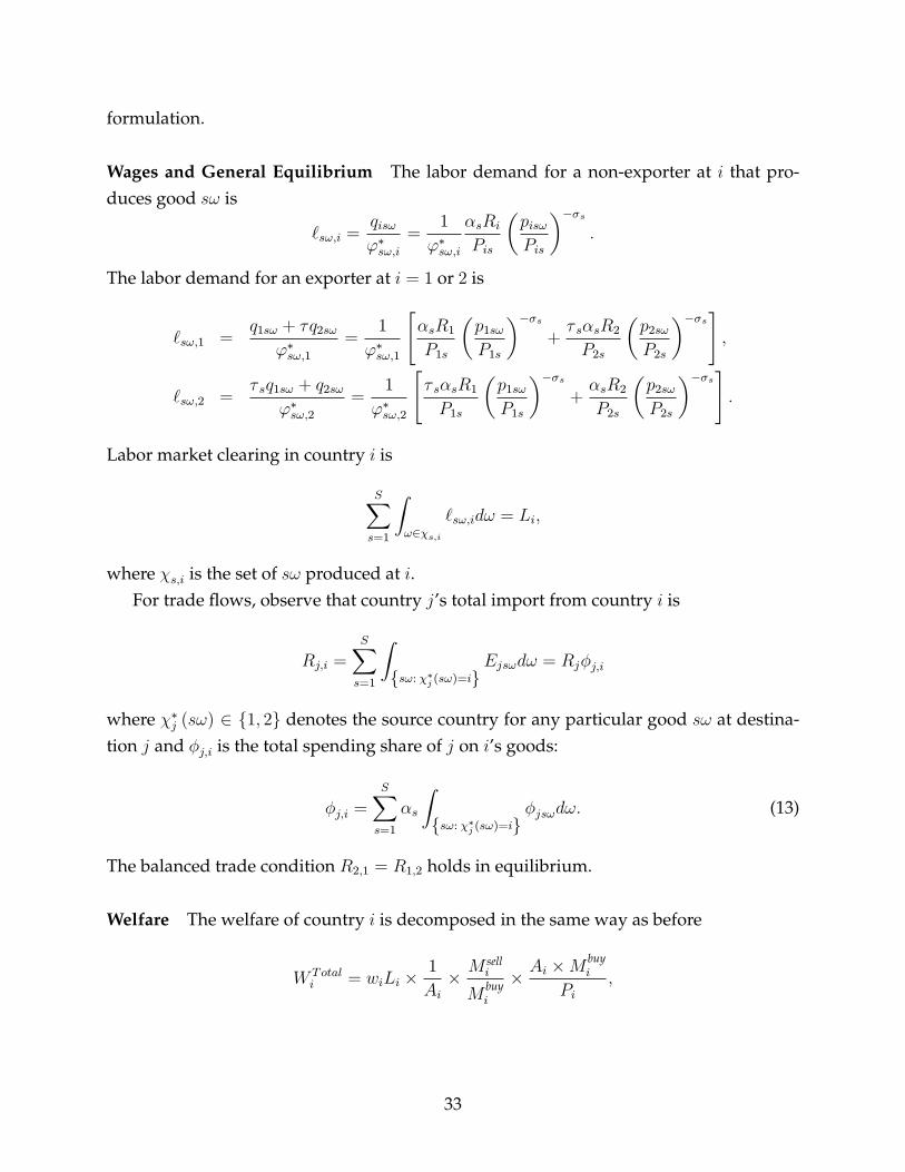
formulation.

Wages and General Equilibrium The labor demand for a non-exporter at i that pro-duces good sω is

`sω,i =qisωϕ∗sω,i

=1

ϕ∗sω,i

αsRi

Pis

(pisωPis

)−σs.

The labor demand for an exporter at i = 1 or 2 is

`sω,1 =q1sω + τq2sω

ϕ∗sω,1=

1

ϕ∗sω,1

[αsR1

P1s

(p1sω

P1s

)−σs+τ sαsR2

P2s

(p2sω

P2s

)−σs],

`sω,2 =τ sq1sω + q2sω

ϕ∗sω,2=

1

ϕ∗sω,2

[τ sαsR1

P1s

(p1sω

P1s

)−σs+αsR2

P2s

(p2sω

P2s

)−σs].

Labor market clearing in country i is

S∑s=1

∫ω∈χs,i

`sω,idω = Li,

where χs,i is the set of sω produced at i.For trade flows, observe that country j’s total import from country i is

Rj,i =S∑s=1

∫{sω: χ∗j (sω)=i}

Ejsωdω = Rjφj,i

where χ∗j (sω) ∈ {1, 2} denotes the source country for any particular good sω at destina-tion j and φj,i is the total spending share of j on i’s goods:

φj,i =

S∑s=1

αs

∫{sω: χ∗j (sω)=i}

φjsωdω. (13)

The balanced trade condition R2,1 = R1,2 holds in equilibrium.

Welfare The welfare of country i is decomposed in the same way as before

W Totali = wiLi ×

1

Ai× M sell

i

Mbuyi

× Ai ×M buyi

Pi,

33

where

Ai = ΠSs=1

(Aisαs

)αs, Pi = ΠS

s=1

(Pisαs

)αs,

Mbuyi =

(S∑s=1

αs

(M

buyis

)−1)−1

, M selli =

Ri

wiLi=

(S∑s=1

Rs,i

Ri

(M sell

is

)−1

)−1

, (14)

and Ais, Pis, and Mbuyis are defined in the same way as before, and M sell

is is

M sellis =

(∫{ω: χ∗s1(ω)=i}

m−11sω

αsR1φ1sω

Rs,i

dω +

∫{ω: χ∗s2(ω)=i}

m−12sω

αsR2φ2sω

Rs,i

dω

)−1

. (15)

The sectoral welfare cannot be further decomposed into the three components as inthe one-sector model. This breaks down because there is no simple analogue of Ri =

wiLi ×M selli at the sectoral level. Indeed, wiLi =

∑sRisM sellis

.

Quantifying the Model To quantify the model, we focus on 29 2-digit manufacturingsectors in Chinese Industrial Classifications (CIC).34 We first calibrate {αs}Ss=1. Recall thatP1sQ1s = αsR1. We use information about expenditure share in China’s 1997 and 2002input-output table to calibrate αst, where t = 1997, 2002. We then set αs to be the averagebetween two years.35 We then follow the same procedure as in the one-sector economycase to infer the elasticity of substitution σs and estimate the remaining parameters bySMM using sectoral firm-level data. Note that one convenience in our framework is thatto implement SMM, moments are generated given wages w and total revenue R1 and R2,and each sector is actually estimated separately, which largely simplifies the estimationand equilibrium computation for counter-factuals.

The parameter estimates are shown in Tables 10A and 10B. In both tables, we alsoreport the (unweighted) mean, standard deviation, maximum and minimum of the es-timates and percentage changes across sectors. There are substantial variations acrossindustries in their moments. The model performs well in accommodating these varia-tions with corresponding variations in the estimates. The changes in the unweightedmeans of parameters between 1995 and 2004 are all consistent with the pattern observedin the one-sector case, except for the parameter η1 (see Table 2). In particular, all esti-

34We include all 2-digit CIC manufacturing sectors except Sector 43 because we do not have the necessarydata to calculate markups for this industry.

35Specifically, we first map the input-output code to 2-digit CIC sectors. Then, we calculate the expendi-ture share for each 2-digit CIC sector, where the expenditure is calculated by subtracting exports from totaluse, which already includes imports.

34

mated trade costs decrease except for Tobacco Processing.36 Also observe that the meanσs is 1.44, which is quite close to our benchmark in the one-sector economy, and σs in mostindustries (23 out of 29) are within one standard deviation from the mean, (1.27, 1.61).

5.2 Gains from Trade

When examining the welfare analysis in the multi-sector economy, we focus on the twokey counter-factuals shown in Table 11. Whereas we changed τ in the one-sector econ-omy, we now change {τ s} for all sectors s from the 2004 values to the 1995 values (or toinhibitive values). The total gains from trade are 7.2% between 1995 and 2004 and 28.2%

from autarky. The contribution of pro-competitive effects here is around 20%, which isslightly smaller than the numbers in Table 4. Similarly, allocative efficiency accounts foralmost all of the pro-competitive effects.

5.3 Did China Liberalize the Right Sectors?

In this subsection, we try to answer the question of whether China liberalized the rightsectors. We examine the relationship between trade liberalization and sectoral consumers’aggregate markup (M buy

1s ) under the 1995 model. That is, if a sector has a higher M buy1s in

1995, do we also actually see a larger degree of trade liberalization between 1995 and2004? The rationale is as follows. Recall from (14) that aggregate markup M

buy1 is a har-

monic mean of sectoral markups (M buy1s ). From both one-sector and multi-sector welfare

analysis, we observe that most pro-competitive gains from trade are due to allocative ef-ficiency. As the overall allocative efficiency depends on the dispersion of markups acrosssectors, if a sector s has higher M buy

1s initially, then allocative efficiency will improve moreif the government targets its trade liberalization more in these higher markup sectors.

A quick examination is to rank the 29 sectors by their values ofM buy1s at 1995 and divide

them into two groups – the first being 15 sectors with the smaller values of M buy1s and the

second being those with the larger values. The weighted average of theM buy1s are then 1.21

and 1.36, respectively. The corresponding weighted average of the changes in trade costsτ s (i.e, ∆τ s = τ s,2004− τ s,1995) are −0.446 and −0.856, respectively. An alternative measureof trade liberalization is the changes in sectoral import tariffs,37 which directly relate tothe WTO entry but do not account for other factors of trade liberalization. In this case, thecorresponding changes are −0.162 and −0.215, respectively. These simple statistics show

36This is mainly because the import and export shares decrease from 0.021 and 0.052 to 0.010 and 0.016in this sector.

37For details of how the sectoral import tariffs are calculated, see Appendix A2.

35

a tendency where the higher the initial level of sectoral markups, the larger the reductionin trade costs (or import tariffs).38

Columns 1 and 5 of Table 12 show similar results by regressing the changes in sectoraltrade costs and in sectoral import tariffs on sectoral markups M buy

1s at 1995.39 Note thatthese descriptive results suffice for our purpose, as we seek only to examine whetherChina on average liberalized the right sectors, smoothing the dispersion of markupsacross sectors, even if this happened by chance. In other words, we do not try to es-tablish causality. Nevertheless, we also examine conditional correlations by followingTrefler (2004) in accounting for factors that may affect the changes in tariffs. Columns 3and 7 show the results when we add controls for log of wage rates, employment, exports,and imports, all at 1995. The rationale of these controls is that they are highly correlatedwith various kinds of protectionism.40 As the share of SOEs is presumably a good indi-cator of protectionism in China, we also add this as a control (see columns 2, 4, 6, and 8).The above-mentioned tendency still remains.41

One often-mentioned merit of trade liberalization (or tariff reduction) is that it is aneasier route to reducing domestic protectionism compared with using domestic indus-trial policies. Before joining the WTO, import tariffs varied greatly in China, but the WTOconditions generally require larger tariff reductions in those industries with higher ini-tial tariffs (see Lu and Yu 2015). We do not know whether the Chinese government hadbenevolent motives and sought to enhance welfare; it could simply be a mechanical resultof China wanting to enter the WTO. In any case, our structural approach allows a wel-fare assessment in the context of sectoral reallocation both in terms of improved overallallocative efficiency (Table 11) and the results in this subsection.

38The tariff data is obtained from World Integrated Trade Solution (WITS), which was developed by theWorld Bank and incorporates trade data from various sources. In particular, we use TRAINS as it coversmore countries and more years. An observation of tariff is an average tariff at HS 6-digit product level.We use “effectively applied rates” (AHS). As WITS does not report China’s import tariffs in 1995, we takeaverages of the 1994 and 1996 tariffs as proxies. In calculating sectoral import tariffs, we use the mappingof HS 6-digit to CIC 2-digit manufacturing sectors using the concordance table from the National Bureau ofStatistics of China. For each sector, we then use imports in the corresponding product or industry from theprevious year (1994 and 2003) as weights to calculate average import tariffs.

39As sector-level data is grouped data from either firms or products, we weight the regressions by tradevolume and imports when the dependent variables are changes in trade cost and import tariffs, respectively.

40For a detailed explanation, see Trefler (2004), p. 878.41All the coefficients on sectoral markup at 1995 are significant except in column 4, which is marginally

insignificant (with a p-value at 0.11). Nevertheless, the value of this coefficient is similar to those in columns1-3. Also, as the sample size is small (29), one should use caution when interpreting the significance levels.

36

6 Conclusion

Using Chinese firm-level data at 1995 and 2004, this paper studies pro-competitive effectsof trade quantitatively under head-to-head competition. The benchmark counter-factualshows that total gains from such improved openness during this period is 9.4%. The pro-competitive effects account for 25.4% of the total gains from trade from 1995 to 2004 and23.3% from autarky to 2004. Allocative efficiency plays a much more important role thanthe relative markup effect.

Local to the estimated models in 1995 and 2004, the total gains from trade are largerthan the gains predicted by the ACR formula by 17% and 24%, respectively. The totalgain from the change in trade cost between 1995’s and 2004’s levels is 27% larger than theACR formula. These additional gains are mostly from pro-competitive effects. This is aresult that is absent in models when a firm monopolizes a variety, such as in Arkolakiset al. (2017), EMX, Feenstra and Weinstein (2016), and other monopolistic competitivemodels. Head-to-head competition is the main reason driving this difference, as detailedin Sections 2.6 and 4.2.

Overall speaking, total gain from trade is relatively large compared with other esti-mates in the literature. Besides the fact that there is a large reduction in trade cost duringthis period, the two channels for the larger gains are the above-mentioned finding thatpro-competitive effects increase the total gains and the lower trade elasticities in our esti-mated models in a similar fashion to Simonovska and Waugh (2014b). We find that bothchannels are important, as pro-competitive effects account for 39% and 47% of the twochannels combined at 1995 and 2004, respectively. Similarly, for the change of trade costfrom 1995’s to 2004’s levels, pro-competitive effects account for 49% of the two channelscombined.

When comparing with the symmetric-country case, we find that the gains from tradeand its components are substantially smaller in the symmetric-country case, indicatingthe important role played by the differences in productivities and markups. The factthat the symmetric-country implementation may obscure sizable gains from trade indi-cates the importance of implementing asymmetric-country estimation, especially whenthe country of concern is a developing one, such as China. Our approach of separatingmoments from exporters and non-exporters proves to be instrumental in such an imple-mentation.

How can one think about policy in this model? In our model, λ (mean number ofdraws) reflects domestic industrial/competition policy, but from a welfare point of view,decreasing trade cost τ is similar to increasing λ. In particular, from autarky to a fully inte-

37

grated world, λ increases without changing any domestic industrial/competition policy.If both trade policy and domestic industrial policy are tools that a government can use,which one to use depends on the relative benefits and costs of implementing these poli-cies.

Exploiting the variations in sectoral markups and trade costs, we find that China onaverage liberalized the “right” sectors in the sense that the dispersion of markups is re-duced because there tended to be larger trade liberalization in sectors with higher initialmarkups. Even though we do not know exactly how this happened, to target trade lib-eralization in sectors with higher markups is a useful take-away. This is particularly sowhen it is difficult to eliminate distortions in some industries via domestic measures.

Appendix

A1. Algorithm of Computing Equilibrium

We describe a procedure that reduces three equilibrium conditions in three unknowns{w,R1, R2} to one equation in one unknown w. This is useful for faster computation.

One-Sector Economy First, observe from the definition of the producers’ aggregatemarkup for country 1:

M sell1 =

R1

w1L1

=

(∫{ω: χ∗1(ω)=1}

m−11ωφ1ωdω +

∫{ω: χ∗2(ω)=1}

m−12ωφ2ω

R2

R1

dω

)−1

=

(∫{ω: χ∗1(ω)=1}

m−11ωφ1ωdω +

∫{ω: χ∗2(ω)=1}

m−12ωφ2ω

φ1,2

φ2,1

dω

)−1

,

in which the second line uses the balanced trade condition R2R1

=φ1,2φ2,1

, where φj,i denotethe total spending share of country j’s consumers on good from country i. Note thatφj,i =

∫{ω: χ∗j (ω)=i} φjωdω only depends on relative wage w, but not on R1 and R2. Hence,

M sell1 becomes a function of w only. For any given w, we can calculate M sell

1 (w). Then,given w1 = 1 and L1, we get R1 (w) = M sell

1 (w)L1. For R2, we use the balanced tradecondition again:

R2 (w) =φ1,2

φ2,1

(w)×R1 (w) .

38

In fact, M selli = Ri

wiLiis equivalent to the labor market clearing condition of country i. Next,

we calculate

M sell2 (w) =

(∫{ω: χ∗1(ω)=i}

m−1ω,1φω,1

φ2,1

φ1,2

(w) dω +

∫{ω: χ∗2(ω)=i}

m−1ω,2φω,2dω

)−1

.

Finally, given L2, we can use the market clearing condition of country 2 to solve for w:

M sell2 (w) =

R2 (w)

wL2

.

Given the solution of w, we obtain R1 and R2 via the Ri (w) formula above.

Multiple-Sector Economy The algorithm for calculating an equilibrium in a multiple-sector economy is similar. From (14) and (15), we can derive the following formula forM sell

1 and M sell2 :

M sell1 =

[S∑s=1

αs

(∫{ω: χ∗s1(ω)=1}

m−11sωφ1sωdω +

∫{ω: χ∗s2(ω)=1}

m−12sωφ2sω

φ1,2

φ2,1

dω

)]−1

M sell2 (w) =

[S∑s=1

αs

(∫{ω: χ∗s1(ω)=2}

m−11sωφ1sω

φ2,1

φ1,2

(w) dω +

∫{ω: χ∗s2(ω)=2}

m−12sωφ2sωdω

)]−1

,

in which φj,i is the total spending share of j on i’s goods given in (13). Then, we stillcalculate R1 (w) = M sell

1 (w)L1, R2 (w) =φ1,2φ2,1

(w)× R1 (w), and M sell2 (w) = R2(w)

wL2; the last is

used to pin down equilibrium wage ratio w.

A2. Estimation of Markups

In this subsection, we provide the details for calculating firm markups using DLW’smethod. Specifically, we assume that firm i at time t has the following production tech-nology42

Qit = Fit (Lit, Kit,Mit, ωit) , (16)

where Lit, Kit, and Mit are the inputs of labor, capital and intermediate materials, respec-tively; ωit denotes firm-specific productivity. The production function F (.) is assumed tobe continuous and twice-differentiable with respect to all of its arguments.

42Note that the framework is robust to any arbitrary number of inputs. As we only observe three in-puts (i.e., labor, capital and intermediate materials) in our data, here we focus on production technologyinvolving only these three inputs.

39

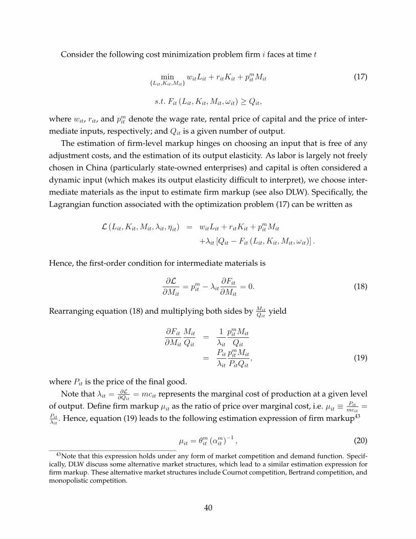
Consider the following cost minimization problem firm i faces at time t

min{Lit,Kit,Mit}

witLit + ritKit + pmitMit (17)

s.t. Fit (Lit, Kit,Mit, ωit) ≥ Qit,

where wit, rit, and pmit denote the wage rate, rental price of capital and the price of inter-mediate inputs, respectively; and Qit is a given number of output.

The estimation of firm-level markup hinges on choosing an input that is free of anyadjustment costs, and the estimation of its output elasticity. As labor is largely not freelychosen in China (particularly state-owned enterprises) and capital is often considered adynamic input (which makes its output elasticity difficult to interpret), we choose inter-mediate materials as the input to estimate firm markup (see also DLW). Specifically, theLagrangian function associated with the optimization problem (17) can be written as

L (Lit, Kit,Mit, λit, ηit) = witLit + ritKit + pmitMit

+λit [Qit − Fit (Lit, Kit,Mit, ωit)] .

Hence, the first-order condition for intermediate materials is

∂L∂Mit

= pmit − λit∂Fit∂Mit

= 0. (18)

Rearranging equation (18) and multiplying both sides by Mit

Qityield

∂Fit∂Mit

Mit

Qit

=1

λit

pmitMit

Qit

=Pitλit

pmitMit

PitQit

, (19)

where Pit is the price of the final good.Note that λit = ∂L

∂Qit= mcit represents the marginal cost of production at a given level

of output. Define firm markup µit as the ratio of price over marginal cost, i.e. µit ≡ Pitmcit

=Pitλit

. Hence, equation (19) leads to the following estimation expression of firm markup43

µit = θmit (αmit )−1 , (20)

43Note that this expression holds under any form of market competition and demand function. Specif-ically, DLW discuss some alternative market structures, which lead to a similar estimation expression forfirm markup. These alternative market structures include Cournot competition, Bertrand competition, andmonopolistic competition.

40

where θmit ≡ ∂Fit∂Mit

Mit

Qitis the output elasticity of intermediate materials and αmit ≡

pmitMit

PitQitis

the share of the expenditure of intermediate materials in total revenue.As the information about the expenditure on intermediate materials and total revenue

is available in the data, αmit can be readily calculated. However, the output elasticity ofintermediate materials, θmit , must be obtained by estimating the production function (16).There is a large literature on the estimation of the production function focusing on how tocontrol for unobserved productivity shocks (for a review, see Ackerberg, Benkard, Berryand Pakes 2007). The solutions range from the instrumental variable estimation to theGMM estimation, and to the control function approach proposed by Olley and Pakes(1996). We adopt the control function approach developed by Ackerberg, Caves and Fra-zier (2006), which comprises a two-step estimation.

Similar to DLW, we assume a translog production function when estimating markups.Specifically, the production function to be estimated is expressed as

qit = βllit + βkkit + βmmit + βlll2it + βkkk

2it + βmmm

2it

+βlklitkit + βkmkitmit + βlmlitmit

+βlkmlitkitmit + ωit + εit, (21)

where the lowercase letters represent the logarithm of the uppercase letters; ωit is firm-specific productivity; and εit is an i.i.d. error term. β= (βl, βk, βm, βll, βkk, βmm, βlk, βkm, βlm, βlkm)

is the vector of production function coefficients.To proxy ωit, Levinsohn and Petrin (2003) assume that

mit = mt (kit, ωit, exit) ,

where exit denotes the exporter status (i.e. taking value 1 if exporters and 0 otherwise).Given the monotonicity of mt (.), we have

ωit = ht (mit, kit, exit) .

In the first stage, we estimate the following equation

qit = φit + εit,

41

where

φit = βllit + βkkit + βmmit + βlll2it + βkkk

2it + βmmm

2it

+βlklitkit + βkmkitmit + βlmlitmit + βlkmlitkitmit + ht (mit, kit, exit) ,

and obtain the estimates of the expected output (φit) and the error term (εit).Meanwhile, to recover all the production function coefficients β in the second stage,

we model firm productivity as following a first-order Markov movement, i.e.

ωit = gt (ωit−1) + ξit,

where ξit is an idiosyncratic shock.From the first stage, the productivity for any given value of β can be computed as

ωit (β) = φit −(

βllit + βkkit + βmmit + βlll2it + βkkk

2it + βmmm

2it

+βlklitkit + βkmkitmit + βlmlitmit + βlkmlitkitmit

).

The idiosyncratic shock to productivity given β, ξit (β), can then be obtained through anon-parametric regression of ωit (β) on ωit−1 (β).

To identify the coefficients of the production function, Ackerberg, Caves and Frazier(2006) assume that capital is determined one period beforehand and hence is not corre-lated with ξit (β). Meanwhile, wage rates and prices of intermediate materials are as-sumed to vary across firms and be serially correlated.

Therefore, the moment conditions used to estimate the coefficients of the productionfunction are

E (ξit (β)Y′it) = 0,

whereYit = {lit−1, l2it−1,mit−1,m

2it−1, kit, k

2it, lit−1mit−1, lit−1kit,mit−1kit, lit−1mit−1kit}.

We estimate the translog production function (21) separately for each 2-digit industryusing the Annual Survey of Manufacturing Firms conducted by the NBS from 1998 to2005. Specifically, we use the logarithm of sales deflated by 2-digit ex-factory price indicesto measure qit, the logarithm of employment to measure lit, the logarithm of the net valueof fixed assets deflated by investment price indices to measure kit, and the logarithm ofintermediate materials44 deflated by input price indices to measuremit; both price indicesare provided by Brandt, Van Biesebroeck and Zhang (2012).

44The value of intermediate materials is calculated as (production costs)−(total wages)−(total welfarebenefits)−(current-year depreciation)×(production costs)/(production costs+selling costs+administrativecosts+financial costs).

42

Once β =(βl, βk, βm, βll, βkk, βmm, βlk, βkm, βlm, βlkm

)is obtained, we can readily cal-

culate the firm markup using equation (20), i.e.

µit = θm

it (αmit )−1 ,

where θm

it = βm + 2βmmmit + βlmlit + βkmkit + βlmklitkit. Production estimates are reportedin Table A1.

A3. Welfare Gains by the ACR Formula with Large Change in Trade

Cost

We first calculate

lnWACR,2004j

WACR,1995j

=

∫ τ2004

τ1995

d lnWACRj (τ) =

∫ τ2004

τ1995

d

(ln vjj (τ)

ε (τ)

).

To numerically calculate the above, we discretize the interval of [τ 2004, τ 1995] by havingan n-grid so that τ 0 = τ 1995, τ 1 = τ 1995 − τ1995−τ2004

n,..., τ i = τ 1995 − i × τ1995−τ2004

n,..., and

τn = τ 2004. The ACR formula for this large change in trade cost is thus calculated by

lnWACR,2004j

WACR,1995j

≈n∑i=1

1

εi[ln vjj (τ i)− ln vjj (τ i−1)] .

We calculate vjj (τ i) precisely at τ i, and we calculate the trade elasticity εi on each i-th gridusing the two-point formula mentioned in footnote 28 at τ = τ i−1+τ i

2. For our numerical

calculation, we use n = 50 so that the grid size is (2.311− 1.664) /50 = 0.01294. Once we

obtain ln

(WACR,2004j

WACR,1995j

), we can then calculate the percentage increase in welfare

WACR,2004j

WACR,1995j

− 1.

A4. Model with Trade Imbalance

To model trade imbalance, we follow the literature by allowing an exogenous trade deficitDi for each country i with the requirement that D1 +D2 = 0. The total income in countryi is therefore Yi = Ri + Di. As China has a trade surplus in both years, we can set hereD2 = D > 0 and D1 = −D, where D is the size of surplus in China.

Labor demand in country i from a non-exporter that produces input ω is

`ω,i =qiωϕ∗ω,i

=1

ϕ∗ω,i

Ri +Di

Pi

(piωPi

)−σ.

43

For an exporter at i, its labor demand is

`ω,1 =q1ω + τq2ω

ϕ∗ω,1=

1

ϕ∗ω,1

[R1 −DP1

(p1ω

P1

)−σ+τ (R2 +D)

P2

(p2ω

P2

)−σ]

`ω,2 =τq1ω + q2ω

ϕ∗ω,2=

1

ϕ∗ω,2

[τ (R1 −D)

P1

(p1ω

P1

)−σ+R2 +D

P2

(p2ω

P2

)−σ].

Labor market clearing in country i is again∫ω∈χi

`ω,idω = Li. The previous balanced tradecondition (6) is now modified as (R2 +D)φ2,1 = (R1 −D)φ1,2 +D, or equivalently,

R2φ2,1 = R1φ1,2 +D(φ2,2 − φ1,2

), (22)

where φj,i is the total spending share of j on i’s goods:

φj,i =

∫{ω: χ∗j (ω)=i}

φjωdω.

Similar to Section 2.4, the equilibrium {w,R1, R2} is determined by the two labor marketclearing conditions and (22).

The algorithm for computing equilibrium is more complicated than the benchmarkmodel. First, observe from the definition of the producers’ aggregate markup for country1:

M sell1 =

R1

w1L1

=

∫{ω: χ∗1(ω)=1} φ1ωY1dω +

∫{ω: χ∗2(ω)=1} φ2ωY2dω∫

{ω: χ∗1(ω)=1}m−11ωφ1ωY1dω +

∫{ω: χ∗2(ω)=1}m

−12ωφ2ωY2dω

=

(∫{ω: χ∗1(ω)=1}

m−11ω

φ1ω (R1 −D)

R1

dω +

∫{ω: χ∗2(ω)=1}

m−12ω

φ2ω (R2 +D)

R1

dω

)−1

=

((1− D

R1

)∫{ω: χ∗1(ω)=1}

m−11ωφ1ωdω +

(φ1,2

φ2,1

+D

R1

1− φ1,2

φ2,1

)∫{ω: χ∗2(ω)=1}

m−12ωφ2ωdω

)−1

Recall that φj,i =∫{ω: χ∗j (ω)=i} φjωdω only depends on relative wage w, but not on R1 and

R2. Hence, M sell1 becomes a function of w and R1 only. For any given R1 and w, we can

calculate M sell1 (w,R1). Then, given w1 = 1 and L1, we can solve for R1 as a fixed point in

R1 = M sell1 (w,R1)L1 and obtain R1 (w). For R2, we use (22) again:

R2 (w) = R1 (w)φ1,2

φ2,1

+D

(1− φ1,2

φ2,1

− 1

).

44

In fact, M selli = Ri

wiLiis equivalent to the labor market clearing condition of country i. Next,

we calculate

M sell2 (w) =

(R1 (w)−DR2 (w)

∫{ω: χ∗1(ω)=i}

m−11ωφ1ωdω +

R2 (w) +D

R2 (w)

∫{ω: χ∗2(ω)=i}

m−12ωφ2ωdω

)−1

,

Finally, given L2, we can use the market clearing condition of country 2 to solve for w:

M sell2 (w) =

R2 (w)

wL2

.

Given the solution of w, equilibrium R1 and R2 can be obtained using the above proce-dure.

The SMM result of the modified model is presented in Table A2.

45

References

Ackerberg, D., C. L. Benkard, S. Berry, and A. Pakes (2007), “Econometric Tools for Ana-lyzing Market Outcomes" in Handbook of Econometrics, Volume 6A, ed. James J. Heck-man and Edward E. Leamer, 4171–276. Amsterdam and Boston: Elsevier, North-Holland.

Ackerberg, D., K. Caves, and G. Frazer (2006), “Structural Identification of ProductionFunctions", working paper, UCLA.

Alvarez, Fernando and Robert Jr. Lucas (2007), "General Equilibrium Analysis of theEaton-Kortum model of International Trade," Journal of Monetary Economics, 54(6): 1726-1768.

Arkolakis, C., A. Costinot, and A. Rodriguez-Clare (2012), “New Trade Models, Same OldGains?,” American Economic Review, 102(1): 94–130.

Arkolakis, C., A. Costinot, D. Donaldson, and A. Rodriguez-Clare (2017), “The ElusivePro-Competitive Effects of Trade,” working paper, Yale University, February 2017.

Asturias, Jose, Manuel García-Santana, and Roberto Ramos (2017), “Competition and theWelfare Gains from Transportation Infrastructure: Evidence from the Golden Quadri-lateral of India,” working paper, Georgetown University Qatar.

Atkeson, A., and A. Burstein (2008), “Pricing to Market, Trade Costs, and InternationalRelative Prices,” American Economic Review, 98(5): 1998–2031.

Behrens, K., and Y. Murata, (2012) “Trade, Competition, and Efficiency,” Journal of Inter-national Economics, 87(1): 1-17.

Bernard, A. B., J. Eaton, J. B. Jensen, and S. Kortum (2003), “Plants and Productivity inInternational Trade,” American Economic Review, 93(4): 1268–1290.

Brandt, L., J. Van Biesebroeck, L. Wang and Y. Zhang (2012), “WTO Accession and Perfor-mance of Chinese Manufacturing Firms,” working paper, Department of Economics,University of Toronto.

Brandt, L., J. Van Biesebroeck, Y. Zhang (2012), "Creative Accounting or Creative Destruc-tion: Firm Level Productivity Growth in Chinese Manufacturing", Journal of Develop-ment Economics, 97(2): 339–351.

Caliendo, L. and F. Parro (2015), “Estimates of the Trade and Welfare Effects of NAFTA,”Review of Economic Studies, 82(1): 1-44.

de Blas, B., and K. Russ (2015), “Understanding Markups in the Open Economy underBertrand Competition,” American Economic Journal: Macroeconomics, 7(2): 157-80.

di Giovanni, J., A. A. Levchenko and J. Zhang (2014), “The Global Welfare Impact ofChina: Trade Integration and Technological Change,” American Economic Journal: Macro-

46

economics, 6(3): 153-183.De Loecker, J. and F. Warzynski (2012), “Markups and Firm-level Export Status,” American

Economic Review, 102(6): 2437-2471.Devereux, M. B and K. M. Lee (2001), “Dynamic Gains from International Trade with

Imperfect Competition and Market Power,” Review of Development Economics, 5(2): 239-255.

Dixit, A. K. and J. E. Stiglitz (1977), “Monopolistic Competition and Optimum ProductDiversity,” American Economic Review, 67(3): 297-308.

Dhingra, S., and Morrow, J. (2016), “Monopolistic Competition and Optimum ProductDiversity Under Firm Heterogeneity,” working paper, London School of Economics.

Eaton, J. and S. Kortum (2002), “Technology, Geography, and Trade,” Econometrica, 70(5):1741–1779.

Eaton, J., S. Kortum, and S. Sotelo (2013), “International Trade: Linking Micro and Macro,”in Advances in Economics and Econometrics: 1st ed. Vol 2. Cambridge: Cambridge Uni-versity Press: 329–370.

Edmond, C., V. Midrigan, and D. Y. Xu (2015), “Competition, Markups, and the Gainsfrom International Trade,” American Economic Review, 105(10): 3183–3221.

Epifani, P., and G. Gancia (2011), “Trade, markup heterogeneity and misallocations,” Jour-nal of International Economics, 83(1): 1-13.

Fajgelbaum, P. D., and Khandelwal, A. K. (2016), “Measuring the unequal gains fromtrade,” Quarterly Journal of Economics, 131(3): 1113-1180.

Feenstra, R. C. (2014), “Restoring the Product Variety and Pro-competitive Gains fromTrade with Heterogeneous Firms and Bounded Productivity,” NBER Working PaperNo. 19833, January 2014.

Feenstra, R. C., and Weinstein, D. E. (2016). “Globalization, Markups and U.S. Welfare,”Journal of Political Economy, forthcoming.

Goldberg, P. K., J. De Loecker, A. K. Khandelwal, and N. Pavcnik (2015), “Prices, Markupsand Trade Reform,” Econometrica, forthcoming.

Head, K., T. Mayer, and M. Thoenig (2014), “Welfare and Trade without Pareto,” AmericanEconomic Review (Papers and Proceedings), 104(5): 310–316.

Helpman, E., M. Melitz, and Y. Rubinstein (2008), “Estimating Trade Flows: Trading Part-ners and Trading Volumes.” Quarterly Journal of Economics 123: 441–487.

Holmes, T. J., W.-T. Hsu, and S. Lee (2014), “Allocative Efficiency, Mark-ups, and theWelfare Gains from Trade," Journal of International Economics, 94(2): 195–206.

Hsieh, C.-T. and P. J. Klenow (2009), “Misallocation and Manufacturing TFP in China andIndia,” Quarterly Journal of Economics, 124(4): 1403–1448.

47

Hsieh, C. T., and Ossa, R. (2016), “A global view of productivity growth in China,” Journalof International Economics, 102: 209-224.

Karabarbounis, L., and B. Neiman (2014), “The Global Decline of the Labor Share,” Quar-terly Journal of Economics, 129(1): 61–103.

Krugman, P. R. (1979), “Increasing returns, monopolistic competition, and internationaltrade,” Journal of international Economics, 9(4): 469-479.

Levinsohn, J. A., and A. K. Petrin (2003), “Estimating Production Functions Using Inputsto Control for Unobservables,” Review of Economic Studies, 70(2): 317–342.

Lipsey, R. G. and Kelvin Lancaster (1956-1957), “The General Theory of Second Best,”Review of Economic Studies, 24(1): 11-32.

Lu, Y. and L. Yu (2015), “Trade Liberalization and Markup Dispersion: Evidence fromChina’s WTO Accession,” American Economic Journal: Applied Economics, 7(4): 221–253.

Markusen, J. (1981), “Trade and the Gains from Trade with Imperfect Competition,” Jour-nal of International Economics, 11: 531-551.

Melitz, M. J. (2003), “The impact of trade on intra-industry reallocations and aggregateindustry productivity,” Econometrica, 71(6): 1695-1725.

Melitz, M. J., and G. Ottaviano (2008), “Market Size, Trade, and Productivity,” Review ofEconomic Studies, 75(1): 295–316.

Melitz, M. J., and S. J. Redding (2015), “New Trade Models, New Welfare Implications,”American Economic Review, 105(3): 1105–46.

Olley, G. S., and A. Pakes (1996), “The Dynamics of Productivity in the Telecommunica-tions Equipment Industry,” Econometrica 64, 1263–1298

Ottaviano, G., T. Tabuchi, and J.-F. Thisse (2002), “Agglomeration and Trade Revisited,"International Economic Review, 43(2): 409–435.

Restuccia, D., and R. Rogerson (2008), “Policy Distortions and Aggregate Productivitywith Heterogeneous Plants,” Review of Economic Dynamics, 11: 707–720.

Robinson, Joan (1934), The Economics of Imperfect Competition, Macmillan.Salvo, A. (2010), “Inferring Market Power under the Threat of Entry: The Case of the

Brazilian Cement Industry,” RAND Journal of Economics, 41(2): 326–350.Schmitz, Jr. J. A. (2005), “What Determines Productivity? Lessons from the Dramatic

Recovery of the U.S. and Canadian Iron Ore Industries Following Their Early 1980sCrisis,” Journal of Political Economy, 113(3): 582–625.

Simonovska, I., and Waugh, M. E. (2014a), “The elasticity of trade: Estimates and evi-dence,” Journal of International Economics, 92(1): 34-50.

Simonovska, I., and Waugh, M. E. (2014b), “Trade models, trade elasticities, and the gainsfrom trade” NBER working paper w20495.

48

Trefler, D. (2004), “The Long and Short of the Canada-U.S. Free Trade Agreement,” Amer-ican Economic Review, 94(4): 870–895.

Weinberger, A. (2015), “Markups and Misallocation with Trade and Heterogeneous Firms,”Globalization and Monetary Policy Institute Working Paper No. 251, Federal ReserveBank of Dallas.

Zhelobodko, E., Kokovin, S., Parenti, M., and Thisse, J. F. (2012), “Monopolistic competi-tion: Beyond the constant elasticity of substitution,” Econometrica, 80(6): 2765-2784.

49

01

23

dens

ity

1 1.5 2 2.5 3markup

19952004

Figure 1: Markup Distributions (1995 versus 2004)

50

Year 1995 2004 1995 2004 1995 2004

Mean 1.428 1.372 1.340 1.318 1.432 1.379

Std. dev. 0.495 0.479 0.431 0.438 0.498 0.483

p1 1.005 1.004 1.003 1.004 1.005 1.004

p5 1.022 1.019 1.017 1.017 1.023 1.019

p10 1.044 1.036 1.034 1.032 1.045 1.037

p25 1.114 1.091 1.084 1.077 1.116 1.093

p50 1.262 1.207 1.120 1.168 1.266 1.213

p75 1.538 1.437 1.414 1.362 1.544 1.447

p90 2.015 1.893 1.784 1.747 2.023 1.909

p95 2.464 2.379 2.199 2.183 2.475 2.400

p99 3.528 3.509 3.299 3.364 3.537 3.523

Table 1: Detailed Markup Distributions

All firms Exporters Non-exporters

51

Predetermined

w Relative wages (the ROW to China)

R1 China's manufacturing sales ($b)

R2 ROW's manufacturing sales ($b)

σ Inferred from p99 markup

Moments for SMM Data Model Data Model

import share 0.130 0.144 0.222 0.262

export share 0.153 0.190 0.249 0.277

relative number of firms 0.210 0.219 0.596 0.616

fraction of exporters 0.044 0.024 0.105 0.062

mean cost share for exporters 0.845 0.798 0.801 0.804

std of cost share for exporters 0.135 0.142 0.142 0.124

p50 markup for exporters 1.120 1.212 1.168 1.203

p95 markup for exporters 2.199 2.457 2.183 1.839

mean cost share for non-exporters 0.789 0.712 0.829 0.775

std of cost share for non-exporters 0.147 0.187 0.139 0.152

p50 markup for non-exporters 1.266 1.391 1.213 1.264

p95 markup for non-exporters 2.475 2.775 2.400 2.056

Estimates s.e.  Estimates s.e. 

2.311 0.020 1.664 0.005

0.261 0.002 0.849 0.005

2.442 0.062 2.607 0.040

5.286 0.061 5.828 0.063

-2.401 0.024 -1.785 0.009

0.444 0.008 0.410 0.001

0.349 0.016 0.293 0.011

Simulated macro variables under estimated parameters Data Model Data Model

w 10.5 10.3 5.3 5.3

R1 918,291 954,812 2,343,328 2,398,028

R2 9,397,500 8,410,637 14,737,500 13,974,893

η_2, std of log productivity, ROW

Notes: All units, if any, are in billions USD, current price. The import share is the import penetration ratio, i.e. IM/(R1-EX+IM),

and the export share is the total export divided by the same denominator. All the cost share moments are weighted by firms'

revenues. Recall that a firm's cost share is the inverse of its markup. p# denotes the #-th percentile.

14,737,500

1.40

μ_1, mean of log productivity, China relative to ROW

η_1, std of log productivity, China

λ_1, Poisson parameter, China

λ_2, Poisson parameter, ROW

Parameter values

τ, trade cost

γ/ , measure of goods relative to

9,397,500

1.40

918,291 2,343,328

Table 2: SMM Results

1995 2004

10.5 5.3

52

moments τ γ λ_1 λ_2 μ_1 η_1 η_2

import share -0.514 0.005 -0.076 0.002 -0.246 -0.004 0.586

export share -0.977 0.007 0.087 -0.070 1.169 0.726 -0.345

relative number of firms 0.316 0.775 0.110 -0.013 0.479 0.212 -0.922

fraction of exporters -0.214 0.001 0.007 -0.012 0.154 0.190 -0.026

mean cost share for exporters -0.024 0.001 0.013 0.006 0.026 -0.102 -0.062

std of cost share for exporters 0.009 -0.012 -0.009 -0.012 -0.022 -0.139 0.074

p50 markup for exporters 0.038 0.009 -0.020 -0.005 -0.029 0.168 0.034

p95 markup for exporters 0.369 -0.132 -0.185 -0.164 -0.594 -12.864 1.008

mean cost share for non-exporters -0.109 -0.001 0.019 0.002 -0.066 -0.367 0.092

std of cost share for non-exporters 0.070 -0.001 -0.006 -0.001 0.031 0.186 -0.029

p50 markup for non-exporters 0.176 0.007 -0.037 -0.004 0.141 0.619 -0.189

p95 markup for non-exporters 1.019 -0.031 -0.111 -0.025 0.583 2.772 -0.522

Table 3: Jacobian Matrix

Notes: Each entry of this table gives the rate of change of a moment to a parameter. This is based on the

benchmark estimation of the 2004 model. The larger the absolute value of the rate of change, the more sensitive

this moment is to the parameter, and the more useful this moment is in identifying this parameter.

53

Under 2004

estimates τ at 1995 % change Autarky % change

τ, trade cost 1.664 2.311 1,000,000

Welfare

Total Welfare 1.90E+21 1.73E+21 9.4% 1.42E+21 33.4%

W_Prod 1.04E+15 9.78E+14 6.8% 8.44E+14 23.8%

W_A 0.965 0.945 2.1% 0.897 7.5%

W_R 1.003 1.000 0.3% 1.000 0.3%

Contribution to total welfare

W_A and W_R 25.4% 23.3%

W_A 22.3% 22.4%

Autarky

10% import

share

% change

from autarky

20% import

share

% change

from 10%

import share

τ, trade cost 1,000,000 2.252 1.810

Welfare

Total Welfare 1.42E+21 1.74E+21 22.6% 1.85E+21 6.0%

W_Prod 8.44E+14 9.81E+14 16.2% 1.02E+15 4.3%

W_A 0.897 0.946 5.5% 0.960 1.5%

W_R 1.000 1.000 0.0% 1.002 0.2%

Contribution to total welfare

W_A and W_R 24.2% 27.6%

W_A 24.2% 24.6%

Panel B: Counter-factual from autarky

Notes: In Panel A, all the analysis is done under 2004 estimates, and only the trade cost (τ) changes.

The reported percentage changes in this panel are under the changes from the corresponding τ to

2004's τ. Panel B reports results when τ is changed from an inhibitive level (autarky) to the level that

entails 10%, and then from 10% to 20%, with other parameters fixed at the 2004 estimates.

Panel A: Counter-factual from 2004 estimates

Table 4: Counter-factual Analysis

54

Total

Welfare

Gains

Gains in

Productive

Efficieny

Pro-

competitive

Gains

Contribution

of Pro-

competitive

Effects

Trade

Elasticity

Gains by the

ACR

formula

Additional

gains over

the ACR

formula

1995 0.249 0.194 0.055 22.0% -2.48 0.200 24.3%

2004 0.409 0.330 0.079 19.3% -3.23 0.349 17.1%

`

Table 5: Welfare Analysis Local to the Estimated Model and Comparison with the

ACR Formula

Notes: All the welfare gains here are calculated in terms of welfare elasticity to trade cost, i.e., dln(W)/dln(tau),

where W could be total welfare or its components, or the one according to the ACR formula. For both the 1995

and 2004 models, we calculate the welfare gains and its components from estimated tau to the case where

ln(tau')=ln(tau)-h, where h = 0.001. To reduce secant error in calculating trade elasticity, we use two-point

formula: f'(x) = (f(x+h)-f(x-h))/2h, and here x=ln(tau21) and f = ln((1-v11)/v11). As in ACR, the trade elasticity

calculated here is partial, i.e., wages are fixed at the initial equilibrium.

55

Predetermined

w Relative wages (the ROW to China)

R1 China's manufacturing sales ($b)

R2 ROW's manufacturing sales ($b)

σ Inferred from p99 markup

Moments Data Model Data Model

import share 0.130 0.053 0.222 0.117

export share 0.153 0.049 0.249 0.114

relative number of firms 0.210 0.213 0.596 0.611

fraction of exporters 0.044 0.064 0.105 0.140

mean cost share for exporters 0.845 0.731 0.801 0.747

std of cost share for exporters 0.135 0.158 0.142 0.142

p50 markup for exporters 1.120 1.370 1.168 1.334

p95 markup for exporters 2.199 2.564 2.183 2.052

mean cost share for non-exporters 0.789 0.759 0.829 0.793

std of cost share for non-exporters 0.147 0.170 0.139 0.148

p50 markup for non-exporters 1.266 1.289 1.213 1.230

p95 markup for non-exporters 2.475 2.399 2.400 1.995

Estimate s.e. Estimate s.e.

2.329 0.008 1.738 0.003

0.228 0.002 0.699 0.003

3.635 0.010 4.219 0.080

0.399 0.003 0.407 0.005

Notes: All the units, if any, are in billions USD, current price. For the detailed definition of moments, see Table 2.

λ, Poisson parameter

η, std. of log productivity

Parameter values

τ, trade cost

γ/ , measure of goods relative to

918291 2343328

1.40 1.40

Table 6: SMM Results (Symmetric Countries)

1995 2004

1.0 1.0

918291 2343328

56

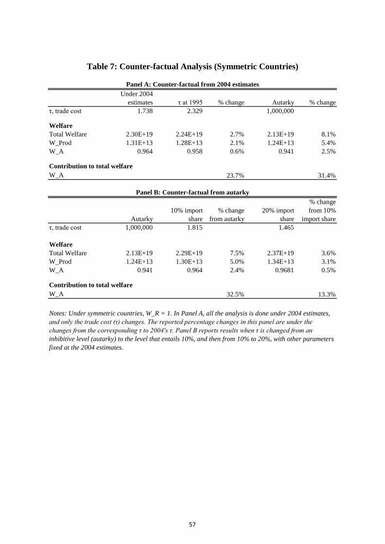
Under 2004

estimates τ at 1995 % change Autarky % change

τ, trade cost 1.738 2.329 1,000,000

Welfare

Total Welfare 2.30E+19 2.24E+19 2.7% 2.13E+19 8.1%

W_Prod 1.31E+13 1.28E+13 2.1% 1.24E+13 5.4%

W_A 0.964 0.958 0.6% 0.941 2.5%

Contribution to total welfare

W_A 23.7% 31.4%

Autarky

10% import

share

% change

from autarky

20% import

share

% change

from 10%

import share

τ, trade cost 1,000,000 1.815 1.465

Welfare

Total Welfare 2.13E+19 2.29E+19 7.5% 2.37E+19 3.6%

W_Prod 1.24E+13 1.30E+13 5.0% 1.34E+13 3.1%

W_A 0.941 0.964 2.4% 0.9681 0.5%

Contribution to total welfare

W_A 32.5% 13.3%

Panel B: Counter-factual from autarky

Notes: Under symmetric countries, W_R = 1. In Panel A, all the analysis is done under 2004 estimates,

and only the trade cost (τ) changes. The reported percentage changes in this panel are under the

changes from the corresponding τ to 2004's τ. Panel B reports results when τ is changed from an

inhibitive level (autarky) to the level that entails 10%, and then from 10% to 20%, with other parameters

fixed at the 2004 estimates.

Panel A: Counter-factual from 2004 estimates

Table 7: Counter-factual Analysis (Symmetric Countries)

57

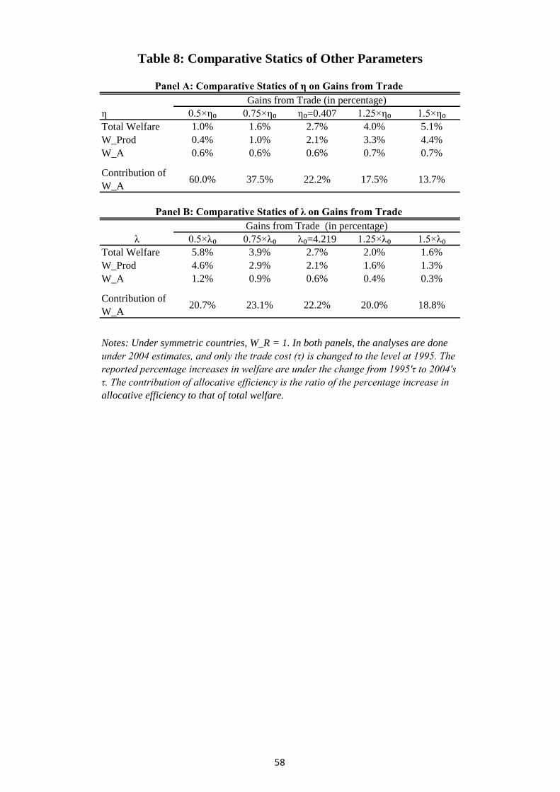
η 0.5×η₀ 0.75×η₀ η₀=0.407 1.25×η₀ 1.5×η₀

Total Welfare 1.0% 1.6% 2.7% 4.0% 5.1%

W_Prod 0.4% 1.0% 2.1% 3.3% 4.4%

W_A 0.6% 0.6% 0.6% 0.7% 0.7%

Contribution of

W_A60.0% 37.5% 22.2% 17.5% 13.7%

λ 0.5×λ₀ 0.75×λ₀ λ₀=4.219 1.25×λ₀ 1.5×λ₀

Total Welfare 5.8% 3.9% 2.7% 2.0% 1.6%

W_Prod 4.6% 2.9% 2.1% 1.6% 1.3%

W_A 1.2% 0.9% 0.6% 0.4% 0.3%

Contribution of

W_A20.7% 23.1% 22.2% 20.0% 18.8%

Table 8: Comparative Statics of Other Parameters

Panel A: Comparative Statics of η on Gains from Trade

Panel B: Comparative Statics of λ on Gains from Trade

Notes: Under symmetric countries, W_R = 1. In both panels, the analyses are done

under 2004 estimates, and only the trade cost (τ) is changed to the level at 1995. The

reported percentage increases in welfare are under the change from 1995'τ to 2004's

τ. The contribution of allocative efficiency is the ratio of the percentage increase in

allocative efficiency to that of total welfare.

Gains from Trade (in percentage)

Gains from Trade (in percentage)

58

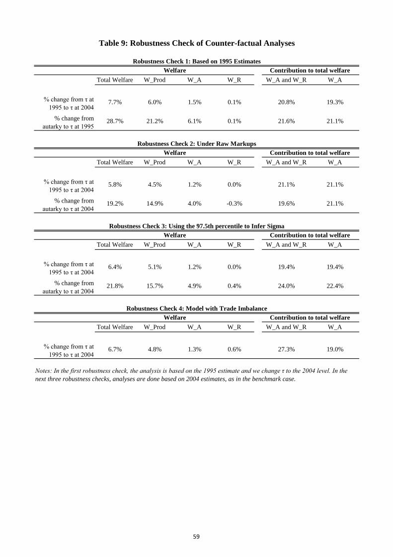
Total Welfare W_Prod W_A W_R W_A and W_R W_A

% change from τ at

1995 to τ at 2004 7.7% 6.0% 1.5% 0.1% 20.8% 19.3%

% change from

autarky to τ at 199528.7% 21.2% 6.1% 0.1% 21.6% 21.1%

Total Welfare W_Prod W_A W_R W_A and W_R W_A

% change from τ at

1995 to τ at 2004 5.8% 4.5% 1.2% 0.0% 21.1% 21.1%

% change from

autarky to τ at 200419.2% 14.9% 4.0% -0.3% 19.6% 21.1%

Total Welfare W_Prod W_A W_R W_A and W_R W_A

% change from τ at

1995 to τ at 2004 6.4% 5.1% 1.2% 0.0% 19.4% 19.4%

% change from

autarky to τ at 200421.8% 15.7% 4.9% 0.4% 24.0% 22.4%

Total Welfare W_Prod W_A W_R W_A and W_R W_A

% change from τ at

1995 to τ at 2004 6.7% 4.8% 1.3% 0.6% 27.3% 19.0%

Contribution to total welfare

Table 9: Robustness Check of Counter-factual Analyses

Robustness Check 1: Based on 1995 Estimates

Notes: In the first robustness check, the analysis is based on the 1995 estimate and we change τ to the 2004 level. In the

next three robustness checks, analyses are done based on 2004 estimates, as in the benchmark case.

Welfare Contribution to total welfare

Robustness Check 2: Under Raw Markups

Welfare

Welfare Contribution to total welfare

Robustness Check 3: Using the 97.5th percentile to Infer Sigma

Welfare Contribution to total welfare

Robustness Check 4: Model with Trade Imbalance

59

cic2d Industry definition σ α 1995 2004 % change 1995 2004 % change 1995 2004 % change 1995 2004 % change

13 Food processing 1.51 0.049 0.018 0.044 139.1 2.47 2.347 -4.9 25.6 16.6 -35.2 1.97 2.01 2.5

14 Food manufacturing 1.33 0.017 0.009 0.018 109.2 4.62 2.49 -46.1 17.5 9.9 -43.6 3.93 2.27 -42.3

15 Beverage manufacturing 1.21 0.014 0.009 0.015 72.4 4.80 3.33 -30.7 25.3 7.7 -69.8 3.83 3.09 -19.3

16 Tobacco processing 1.22 0.014 0.0003 0.0002 -29.8 4.49 4.81 6.9 37.9 9.8 -74.3 3.26 4.38 34.4

17 Textile industry 1.49 0.059 0.013 0.049 269.5 1.88 1.69 -10.4 19.7 7.6 -61.4 1.57 1.57 -0.3

18 Garments & other fiber products 1.37 0.023 0.009 0.028 204.7 3.52 2.91 -17.2 10.8 9.2 -15.0 3.18 2.67 -16.0

19 Leather, furs, down & related products 1.39 0.016 0.006 0.014 136.9 1.96 1.61 -18.0 9.9 5.5 -44.3 1.79 1.53 -14.6

20 Timber processing, bamboo, cane, palm

fiber & straw products1.40 0.011 0.009 0.026 198.8 2.10 1.64 -21.9 7.8 2.6 -67.1 1.95 1.60 -17.9

21 Furniture manufacturing 1.26 0.008 0.005 0.015 215.2 2.47 1.92 -22.2 8.3 1.0 -88.0 2.28 1.90 -16.6

22 Papermaking & paper products 1.48 0.020 0.008 0.025 200.5 2.59 2.16 -16.3 23.7 4.0 -83.0 2.09 2.08 -0.5

23 Printing industry 1.29 0.009 0.010 0.027 157.5 2.68 2.28 -15.1 5.3 0.9 -83.5 2.55 2.26 -11.4

24 Cultural, educational & sports goods 1.35 0.007 0.002 0.009 254.9 2.11 1.72 -18.7 4.1 1.5 -64.3 2.03 1.70 -16.6

25 Petroleum processing & coking 1.45 0.050 0.001 0.006 346.7 1.96 1.54 -21.6 8.6 5.0 -42.2 1.80 1.46 -18.9

26 Raw chemical materials & chemical

products1.50 0.072 0.015 0.073 382.9 2.51 1.74 -30.5 14.6 7.2 -51.0 2.19 1.62 -25.7

27 Medical & pharmaceutical products 1.33 0.017 0.004 0.007 71.9 4.43 2.76 -37.7 6.9 3.8 -44.9 4.15 2.66 -35.8

28 Chemical fiber 2.01 0.010 0.001 0.003 337.5 3.16 2.23 -29.4 22.0 4.9 -77.7 2.59 2.12 -17.9

29 Rubber products 1.50 0.010 0.003 0.009 237.4 2.09 1.84 -11.8 20.2 11.0 -45.6 1.74 1.66 -4.5

30 Plastic products 1.54 0.027 0.011 0.045 320.7 1.76 1.72 -2.4 13.9 5.4 -61.0 1.55 1.63 5.4

31 Nonmetal mineral products 1.35 0.050 0.035 0.094 172.8 4.62 2.39 -48.3 12.8 5.9 -54.0 4.10 2.26 -44.9

32 Smelting & pressing of ferrous metals 1.78 0.092 0.005 0.013 159.1 2.46 2.17 -11.6 10.9 4.9 -55.2 2.22 2.07 -6.6

33 Smelting & pressing of nonferrous metals 1.67 0.031 0.002 0.009 294.3 2.12 1.83 -13.9 7.7 3.9 -49.4 1.97 1.76 -10.7

34 Metal products 1.43 0.032 0.014 0.048 249.6 1.98 1.76 -10.8 13.2 4.0 -69.9 1.75 1.70 -2.8

35 Ordinary machinery 1.50 0.052 0.017 0.084 393.0 3.07 1.64 -46.6 17.5 5.1 -71.0 2.61 1.56 -40.3

36 Special purpose equipment 1.35 0.030 0.011 0.038 241.5 2.41 1.61 -33.2 16.6 5.3 -68.2 2.07 1.53 -26.0

37 Transport equipment 1.36 0.076 0.014 0.036 161.0 2.62 2.18 -16.8 43.5 12.7 -70.8 1.83 1.93 5.9

39 Electric equipment & machinery 1.51 0.061 0.012 0.037 197.9 1.71 1.53 -10.5 11.3 3.0 -73.0 1.54 1.48 -3.4

40 Electronic & telecommunications

equipment1.34 0.121 0.005 0.017 271.3 2.19 1.51 -31.1 13.5 1.3 -90.5 1.93 1.49 -22.8

41 Instruments, meters, cultural & office

equipment1.35 0.013 0.004 0.012 194.4 1.85 1.52 -18.2 15.7 4.3 -72.6 1.60 1.45 -9.2

42 Other manufacturing 1.32 0.009 0.006 0.016 173.0 2.30 1.68 -26.9 8.8 2.8 -67.8 2.12 1.64 -22.7

Mean 1.44 0.034 0.01 0.03 211.52 2.72 2.09 -21.23 15.64 5.74 -61.87 2.35 1.97 -13.77

Standard

deviation0.17 0.029 0.01 0.02 95.89 0.96 0.70 13.23 9.12 3.66 17.25 0.80 0.62 16.52

Max 2.01 0.121 0.03 0.09 392.98 4.80 4.81 6.95 43.46 16.57 -14.99 4.15 4.38 34.39

Min 1.21 0.007 0.00 0.00 -29.81 1.71 1.51 -48.28 4.08 0.87 -90.54 1.54 1.45 -44.90

γ

Table 10A: Estimation Result in Multi-Sector Model (Part A)

τ Tariff Non-tariff τPredetermined

60

cic2d Industry definition 1995 2004 % change 1995 2004 % change 1995 2004 % change 1995 2004 % change 1995 2004 % change

13 Food processing 2.78 3.05 9.9 5.40 6.9 26.8 -2.37 -1.67 29.8 0.43 0.46 8.2 0.38 0.37 -4.8

14 Food manufacturing 3.03 3.11 2.5 4.25 4.6 8.7 -1.51 -1.50 0.7 0.15 0.34 136.2 0.33 0.34 0.2

15 Beverage manufacturing 3.05 3.24 6.2 5.82 4.5 -23.1 -1.20 -1.23 -2.7 0.11 0.22 95.7 0.09 0.16 82.1

16 Tobacco processing 2.75 3.18 15.8 6.00 5.6 -6.3 -2.38 -1.33 44.0 0.34 0.44 28.6 0.27 0.20 -23.6

17 Textile industry 3.04 3.25 6.9 5.73 6.3 10.2 -2.36 -1.78 24.6 0.35 0.38 9.2 0.35 0.17 -50.8

18 Garments & other fiber products 3.03 3.22 6.2 5.27 6.6 25.5 -2.15 -0.93 56.7 0.55 0.42 -23.9 0.11 0.42 269.7

19 Leather, furs, down & related products 2.85 3.21 12.7 5.13 4.6 -10.4 -2.19 -1.75 20.1 0.33 0.37 11.1 0.44 0.26 -40.3

20 Timber processing, bamboo, cane, palm

fiber & straw products2.85 2.98 4.7 5.26 5.4 2.7 -2.40 -1.74 27.5 0.41 0.32 -20.0 0.40 0.25 -38.7

21 Furniture manufacturing 2.51 2.87 14.4 5.53 5.0 -9.6 -2.03 -1.66 18.1 0.24 0.37 56.4 0.26 0.08 -70.6

22 Papermaking & paper products 3.02 2.76 -8.4 5.59 6.1 9.1 -2.33 -1.79 23.3 0.29 0.41 43.3 0.52 0.44 -16.4

23 Printing industry 2.97 2.61 -12.2 6.41 5.6 -12.7 -2.37 -1.78 24.9 0.35 0.42 18.7 0.09 0.18 106.3

24 Cultural, educational & sports goods 2.44 3.02 23.9 5.06 4.6 -8.6 -2.14 -1.70 20.5 0.38 0.42 9.0 0.28 0.15 -46.4

25 Petroleum processing & coking 2.70 2.87 6.3 5.37 6.1 13.8 -2.25 -1.84 18.3 0.21 0.32 51.8 0.36 0.32 -12.3

26 Raw chemical materials & chemical

products2.63 1.97 -25.1 4.84 6.7 39.0 -2.52 -1.92 23.7 0.43 0.51 17.1 0.52 0.36 -31.1

27 Medical & pharmaceutical products 2.99 2.66 -11.1 6.23 5.0 -19.4 -2.09 -1.61 23.1 0.54 0.50 -8.3 0.17 0.39 130.7

28 Chemical fiber 2.44 2.89 18.2 5.47 4.5 -17.6 -2.59 -1.75 32.5 0.46 0.26 -43.3 0.51 0.44 -14.5

29 Rubber products 3.36 2.61 -22.3 5.57 4.6 -18.2 -2.27 -1.72 24.0 0.30 0.37 22.5 0.15 0.15 5.1

30 Plastic products 2.73 3.13 14.6 5.31 5.8 9.1 -2.39 -1.67 30.2 0.31 0.34 11.0 0.21 0.26 22.6

31 Nonmetal mineral products 3.03 3.03 0.1 4.95 5.6 12.5 -1.59 -1.39 12.7 0.25 0.28 11.0 0.20 0.34 65.3

32 Smelting & pressing of ferrous metals 2.87 3.16 10.1 6.50 4.4 -32.5 -2.40 -1.60 33.3 0.06 0.10 59.4 0.34 0.40 20.0

33 Smelting & pressing of nonferrous metals 2.29 2.54 11.2 5.83 5.8 -0.6 -2.46 -1.77 28.1 0.36 0.40 9.5 0.23 0.33 41.7

34 Metal products 3.03 2.83 -6.7 5.54 5.8 5.2 -2.42 -1.82 24.6 0.37 0.39 5.1 0.24 0.09 -60.4

35 Ordinary machinery 2.24 2.50 11.6 4.64 7.3 56.7 -2.44 -1.79 26.8 0.40 0.42 3.8 0.52 0.31 -39.9

36 Special purpose equipment 2.12 2.49 17.3 5.17 6.9 33.3 -2.63 -1.80 31.4 0.34 0.40 19.4 0.52 0.42 -19.5

37 Transport equipment 2.74 2.53 -7.6 6.12 5.9 -3.9 -2.38 -1.72 27.5 0.38 0.42 8.6 0.29 0.30 6.2

39 Electric equipment & machinery 2.44 2.95 20.9 5.93 5.9 0.0 -2.43 -1.77 27.0 0.31 0.40 28.5 0.16 0.34 114.4

40 Electronic & telecommunications

equipment2.41 2.47 2.5 5.81 5.9 1.8 -2.36 -1.77 25.1 0.51 0.53 3.5 0.52 0.44 -16.0

41 Instruments, meters, cultural & office

equipment2.38 2.18 -8.7 4.95 5.8 16.2 -2.41 -1.75 27.5 0.45 0.46 1.9 0.51 0.44 -13.4

42 Other manufacturing 2.73 3.20 17.4 5.36 5.8 8.7 -2.25 -1.74 22.7 0.52 0.43 -17.6 0.34 0.16 -52.4

Mean 2.74 2.84 4.52 5.48 5.64 4.02 -2.25 -1.67 25.03 0.35 0.38 19.19 0.32 0.29 10.80

Standard

deviation0.30 0.34 12.66 0.52 0.81 19.75 0.32 0.21 10.82 0.12 0.09 35.61 0.14 0.11 72.80

Max 3.36 3.25 23.89 6.50 7.27 56.75 -1.20 -0.93 56.74 0.55 0.53 136.22 0.52 0.44 269.74

Min 2.12 1.97 -25.11 4.25 4.39 -32.53 -2.63 -1.92 -2.72 0.06 0.10 -43.25 0.09 0.08 -70.59

Table 10B: Estimation Result in Multi-Sector Model (Part B)

λ_1 λ_2 μ_1 η_1 η_2

61

Total Welfare W_Prod W_A W_R W_A and W_R W_A

% change from τ at

1995 to τ at 2004 7.2% 5.7% 1.4% 0.0% 20.0% 19.7%

% change from

autarky to τ at 200428.2% 21.1% 5.9% -0.1% 20.6% 20.9%

Notes: Similar to Table 4, all the analyses in Panel A are done under 2004 estimates, and only the trade costs change. The

reported percentage changes in this panel are under the changes from the corresponding τ to 2004's.

Table 11: Counter-factual Analysis in Multiple-Sector Economy

Welfare Contribution to total welfare

62

Dependent variable

(1) (2) (3) (4) (5) (6) (7) (8)

Sectoral markup at

1995-2.109** -1.774** -1.980* -1.856 -0.343** -0.378** -0.581* -0.596*

(0.799) (0.833) (1.063) (1.117) (0.154) (0.164) (0.296) (0.303)

SOE share 0.242 -0.967 -0.029 0.042

(0.157) (0.728) (0.032) (0.171)

Log wage at 1995 -0.072 -0.056 -0.065 -0.064

(0.209) (0.218) (0.066) (0.068)

Log employment at

1995-0.153 -0.352 -0.021 -0.011

(0.125) (0.218) (0.029) (0.056)

Log export at 1995 0.166** 0.181** -0.045*** -0.047**

(0.077) (0.087) (0.016) (0.017)

Log import at 1995 -0.035 0.060 0.047** 0.044*

(0.063) (0.116) (0.020) (0.024)

R2 0.169 0.186 0.386 0.449 0.108 0.114 0.363 0.366

Table 12: Did China Liberalize the Right Sectors?

Changes in trade costs between 1995 and 2004 Changes in import tariffs between 1995 and 2004

Notes : The regression is weighted by sectoral trade volume and sectoral imports when the dependent variable is the change in

trade cost and import tariff, respectively. Note that the sample size is small (29), and hence one should use caution when

interpreting the significance levels.* Significant at the 10 percent level.** Significant at the 5 percent level. *** Significant at

the 1 percent level.

63

Industry Median IQR Median IQR Median IQR Median IQR Median IQR Obs.

Food processing 0.09 [0.07,0.13] 0.03 [0.01,0.05] 0.86 [0.81,0.90] 0.99 [0.98,1.00] 0.99 [0.98,1.00] 104,518

Food manufacturing 0.14 [0.11,0.18] 0.05 [0.02,0.08] 0.82 [0.76,0.87] 1.02 [1.00,1.04] 1.03 [1.00,1.04] 48,295

Beverage manufacturing 0.19 [0.14,0.25] 0.02 [-0.01,0.05] 0.78 [0.71,0.84] 1.01 [0.97,1.04] 1.01 [0.98,1.04] 41,894

Tobacco processing 0.17 [0.03,0.33] 0.24 [0.10,0.35] 0.73 [0.64,0.82] 1.14 [1.05,1.23] 1.14 [1.04,1.22] 731

Textile industry 0.16 [0.11,0.22] 0.04 [0.03,0.05] 0.84 [0.77,0.89] 1.03 [0.99,1.06] 1.02 [0.99,1.05] 113,001

Garments and other fiber products 0.23 [0.15,0.35] 0.05 [0.04,0.07] 0.75 [0.64,0.84] 1.02 [1.00,1.05] 1.02 [1.00,1.05] 72,381

Leather, furs, down and related products 0.20 [0.12,0.28] 0.01 [0.00,0.02] 0.81 [0.73,0.88] 1.01 [1.00,1.03] 1.01 [1.00,1.03] 34,655

Timber processing, bamboo, cane, palm fiber and

straw products0.15 [0.10,0.21] 0.03 [0.03,0.04] 0.83 [0.76,0.88] 1.01 [0.99,1.02] 1.00 [0.99,1.02] 57,283

Furniture manufacturing 0.38 [0.33,0.44] -0.02 [-0.03,0.00] 0.99 [0.90,1.07] 1.37 [1.30,1.44] 1.38 [1.32,1.46] 34,126

Papermaking and paper products 0.26 [0.23,0.29] 0.05 [0.04,0.06] 0.85 [0.80,0.89] 1.15 [1.13,1.19] 1.16 [1.13,1.20] 55,606

Printing industry 0.24 [0.21,0.26] 0.11 [0.08,0.15] 0.86 [0.77,0.94] 1.24 [1.17,1.29] 1.25 [1.18,1.30] 57,993

Cultural, educational and sports goods 0.23 [0.15,0.34] 0.06 [0.05,0.08] 0.79 [0.70,0.86] 1.07 [1.04,1.11] 1.06 [1.04,1.10] 20,987

Petroleum processing and coking 0.10 [0.07,0.14] 0.06 [0.05,0.07] 0.83 [0.78,0.87] 0.99 [0.98,1.00] 0.99 [0.98,1.00] 10,430

Raw chemical materials and chemical products 0.22 [0.18,0.25] 0.04 [0.03,0.05] 0.72 [0.67,0.76] 0.97 [0.96,0.97] 0.96 [0.96,0.97] 108,197

Medical and pharmaceutical products 0.25 [0.18,0.32] 0.19 [0.13,0.26] 0.65 [0.55,0.74] 1.08 [1.04,1.12] 1.08 [1.04,1.11] 17,595

Chemical fiber 0.05 [0.01,0.09] 0.16 [0.15,0.18] 0.73 [0.69,0.76] 0.94 [0.92,0.95] 0.94 [0.92,0.95] 4,925

Rubber products 0.23 [0.19,0.27] 0.06 [0.06,0.07] 0.79 [0.73,0.83] 1.08 [1.06,1.09] 1.07 [1.06,1.09] 20,664

Plastic products 0.14 [0.09,0.19] 0.06 [0.05,0.07] 0.83 [0.77,0.88] 1.01 [1.00,1.03] 1.01 [1.00,1.03] 92,509

Nonmetal mineral products 0.15 [0.09,0.22] 0.05 [0.04,0.06] 0.80 [0.72,0.86] 0.98 [0.97,1.01] 0.98 [0.97,1.00] 226,792

Smelting and pressing of ferrous metals 0.10 [0.07,0.14] 0.03 [0.03,0.04] 0.85 [0.80,0.90] 0.98 [0.97,0.99] 0.98 [0.97,0.99] 29,102

Smelting and pressing of nonferrous metals 0.12 [0.08,0.16] 0.03 [0.03,0.04] 0.84 [0.79,0.88] 0.99 [0.99,1.00] 0.99 [0.99,1.00] 20,671

Metal products 0.17 [0.13,0.23] 0.09 [0.08,0.11] 0.71 [0.66,0.76] 0.97 [0.96,1.00] 0.97 [0.95,0.99] 117,081

Ordinary machinery 0.20 [0.16,0.26] 0.08 [0.06,0.09] 0.80 [0.73,0.85] 1.07 [1.06,1.09] 1.07 [1.06,1.08] 148,586

Special purpose equipment 0.24 [0.22,0.28] 0.08 [0.06,0.10] 0.79 [0.73,0.85] 1.13 [1.09,1.16] 1.13 [1.10,1.16] 77,157

Transport equipment 0.16 [0.11,0.22] 0.07 [0.06,0.09] 0.76 [0.69,0.82] 0.99 [0.99,1.00] 0.99 [0.98,1.00] 75,943

Electric equipment and machinery 0.15 [0.11,0.21] 0.06 [0.05,0.07] 0.79 [0.73,0.84] 1.00 [0.99,1.01] 1.00 [0.99,1.01] 63,631

Electronic and telecommunications equipment 0.23 [0.17,0.30] 0.10 [0.09,0.11] 0.73 [0.65,0.80] 1.06 [1.05,1.08] 1.06 [1.05,1.08] 48,716

Instruments, meters, cultural and office equipment 0.20 [0.13,0.29] 0.09 [0.07,0.10] 0.72 [0.63,0.79] 1.00 [0.97,1.04] 1.00 [0.96,1.03] 25,494

Other manufacturing 0.21 [0.14,0.29] 0.06 [0.04,0.07] 0.78 [0.70,0.84] 1.02 [1.00,1.06] 1.02 [1.00,1.05] 39,978

Table A1: Production Function Estimates

Panel A: Output Elasticity With Respect to … Panel B: Returns to Scale

Materials

Notes: IQR means inter-quartile range. In Panel B, we calculate the r in k^rY=F(kK,kL,kM), where Y,K,L,M are output, capital, labor, and material, respectively. The calculation is local to

the data values and our estimate. The columns under "double" and "triple" are the results when k is chosen to be 2 and 3, respectively.

Double TripleLabor Capital

64

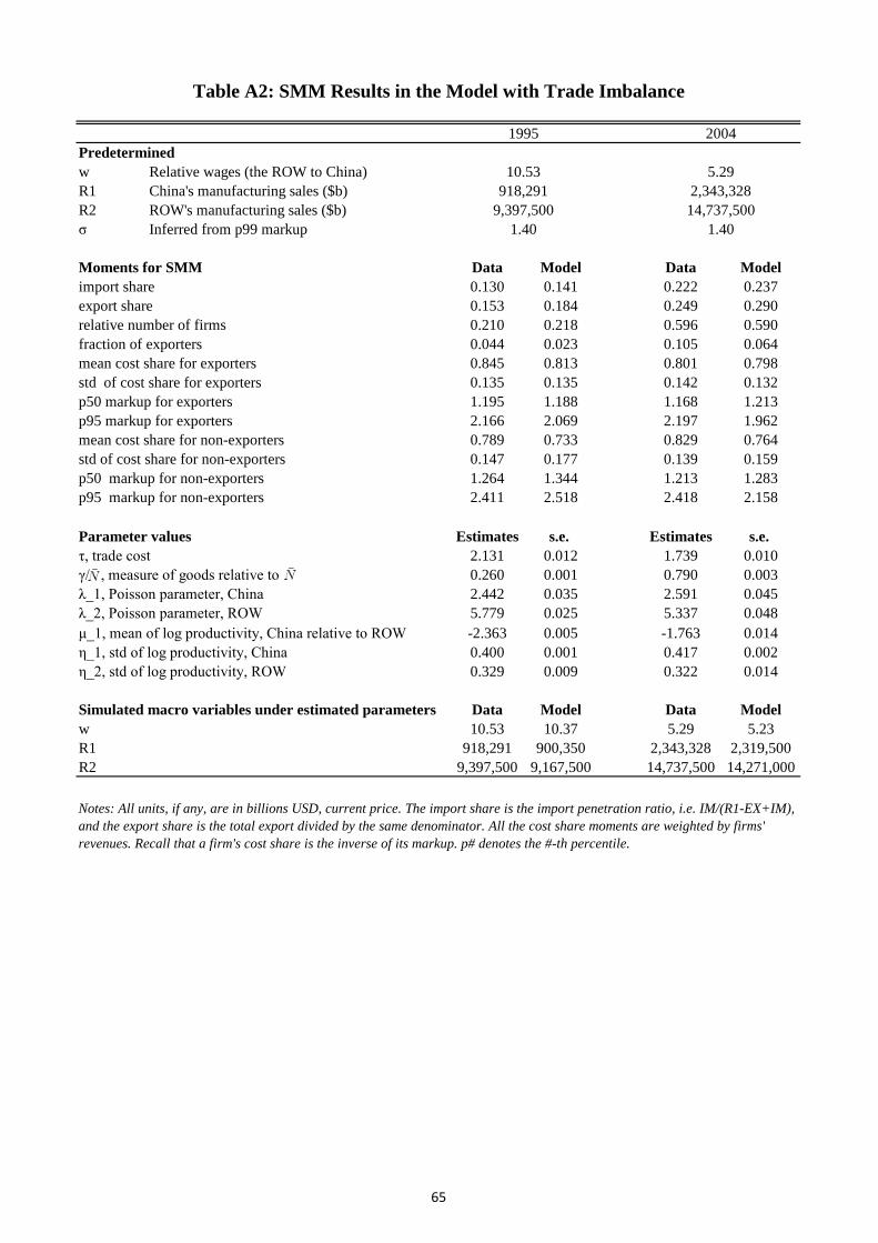
Predetermined

w Relative wages (the ROW to China)

R1 China's manufacturing sales ($b)

R2 ROW's manufacturing sales ($b)

σ Inferred from p99 markup

Moments for SMM Data Model Data Model

import share 0.130 0.141 0.222 0.237

export share 0.153 0.184 0.249 0.290

relative number of firms 0.210 0.218 0.596 0.590

fraction of exporters 0.044 0.023 0.105 0.064

mean cost share for exporters 0.845 0.813 0.801 0.798

std of cost share for exporters 0.135 0.135 0.142 0.132

p50 markup for exporters 1.195 1.188 1.168 1.213

p95 markup for exporters 2.166 2.069 2.197 1.962

mean cost share for non-exporters 0.789 0.733 0.829 0.764

std of cost share for non-exporters 0.147 0.177 0.139 0.159

p50 markup for non-exporters 1.264 1.344 1.213 1.283

p95 markup for non-exporters 2.411 2.518 2.418 2.158

Estimates s.e.  Estimates s.e. 

2.131 0.012 1.739 0.010

0.260 0.001 0.790 0.003

2.442 0.035 2.591 0.045

5.779 0.025 5.337 0.048

-2.363 0.005 -1.763 0.014

0.400 0.001 0.417 0.002

0.329 0.009 0.322 0.014

Simulated macro variables under estimated parameters Data Model Data Model

w 10.53 10.37 5.29 5.23

R1 918,291 900,350 2,343,328 2,319,500

R2 9,397,500 9,167,500 14,737,500 14,271,000

Notes: All units, if any, are in billions USD, current price. The import share is the import penetration ratio, i.e. IM/(R1-EX+IM),

and the export share is the total export divided by the same denominator. All the cost share moments are weighted by firms'

revenues. Recall that a firm's cost share is the inverse of its markup. p# denotes the #-th percentile.

γ/ , measure of goods relative to

λ_1, Poisson parameter, China

λ_2, Poisson parameter, ROW

μ_1, mean of log productivity, China relative to ROW

η_1, std of log productivity, China

η_2, std of log productivity, ROW

τ, trade cost

Table A2: SMM Results in the Model with Trade Imbalance

1995 2004

10.53 5.29

918,291 2,343,328

9,397,500 14,737,500

1.40 1.40

Parameter values

65