COMPARISONS OF APPROXIMATE F TEST AND A PROCEDURE

FOR THE DEVELOPMENT OF AN ALTERNATIVE

by

BARBíjy JA ÎE KEENUM, B.S.

A THESIS

IN

MATHEMATICS

Submitted to the Graduate Faculty of Texas Tech University in Partial Fulfillment of the Requirements for

the Degree of

MASTER OF SCIENCES

Approved

Accepted

August, 1974

TTC

T3

V^tS-lM^4

ACKNOWLEDGEMENTS

I would like to thank Dr. James M. Davenport for hls

assistance in the preparation of this paper and computer

programs used for numerical calculations. I am grateful

to Dr. Truman Lewis for serving on my thesis committee^

I am deeply indebted to Dr. James M. Davenport, Dr^ Thomas

Boullion, Dr^ Benjamin Duran, Dr. Truman Lewis, and Mr.

Jack D. Towery for their guidance and encouragement in my

statistical studies.

ii

CONTENTS

ACKNOWLEDGEMENTS ii

TABLES iv

ILLUSTRATIONS V

I. INTRODUCTION 1

II. EARLIER COMPARITIVE STUDIES 4

III. ADDITIONAL COMPARITIVE STUDIES OF

PROCEDURES FOR TESTING 6 = ®i+®2 ®

IV. MOTIVATION FOR THE DEVELOPEMENT OF

AN IMPROVED PROCEDURE 38

V. CONCLUSIONS AND RECOMENDATIONS 43

REFERENCES 45

APPENDIX 47

111

TABLES

1. Probability of a Type-I Error for Satterthwaite's

Procedure at the Apparent .05 Level

and n^ = 1 13

2. Probability of a Type-I Error for Hoel's

Procedure at the Apparent .05 Level and

nj = 1 13

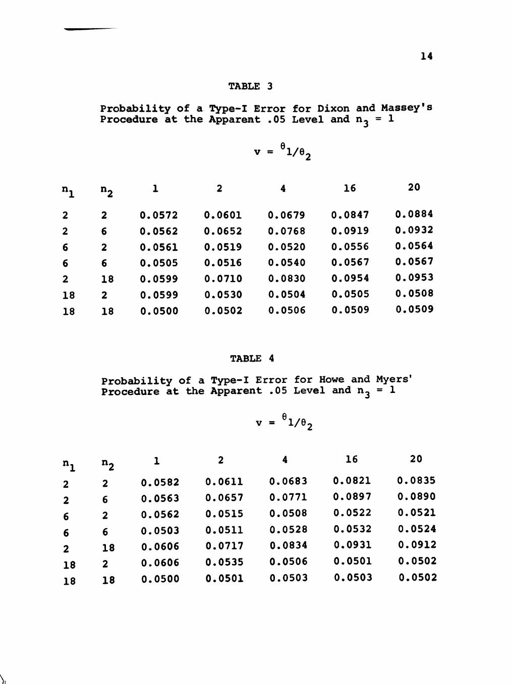
3. Probability of a Type-I Error for Dixon

aná Massey's Procedure at the Apparent •05 Level and n^ = 1 14

4. ProbcdDÍlity of a Type-I Error for Howe and

ítyers' Procedure at the Apparent .05 Level

and n^ = 1 14

5. Probability of Type-I Error for Cochran's

cuid Satterthwaite * s Procedures at the

Apparent .05 Level and n« = 1 35

IV

ILLUSTRATIONS

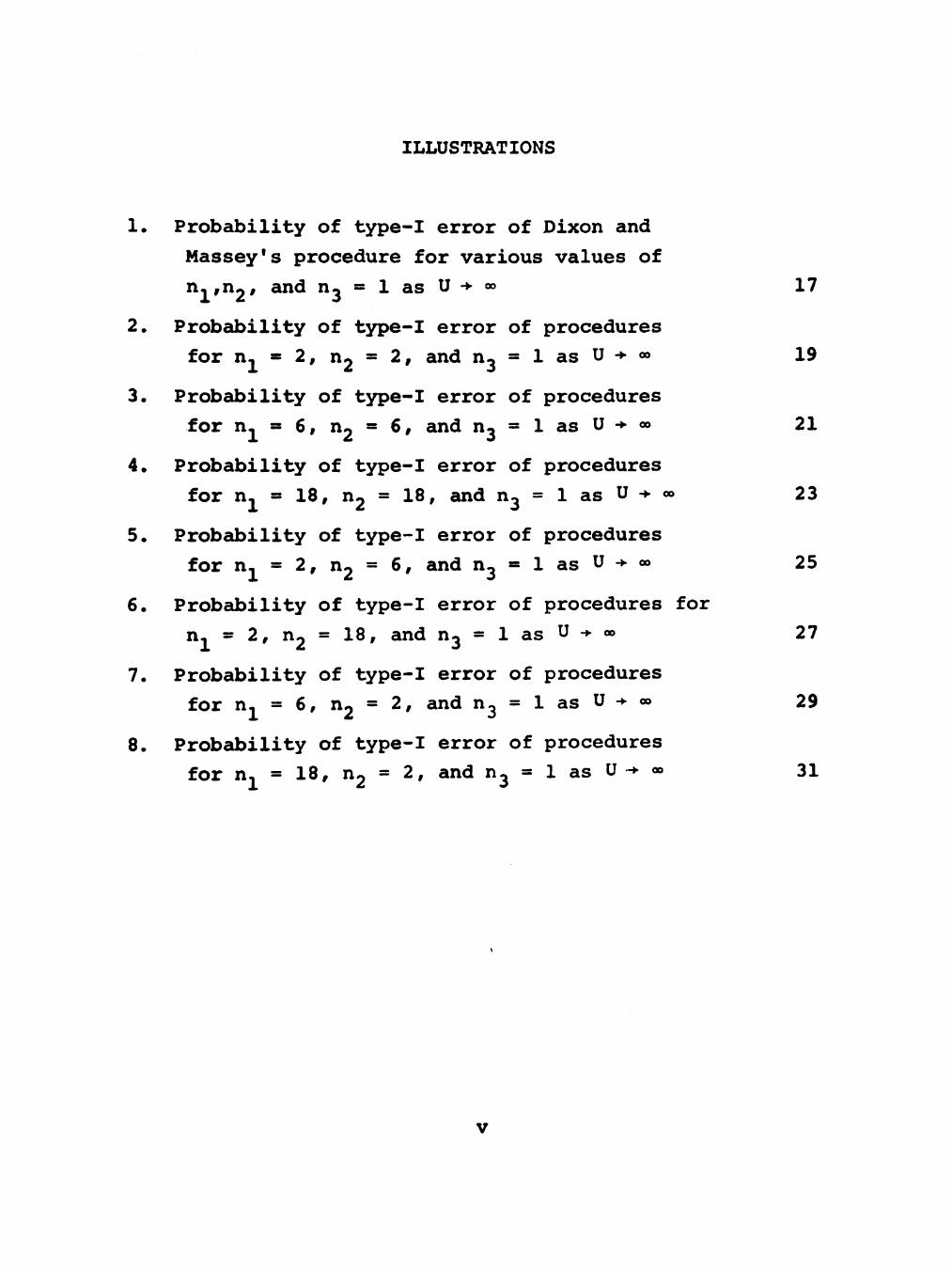
1. Probability of type-I error of Dixon and

Massey's procedure for various values of n.fTi^t and n^ = 1 as U -• » 17

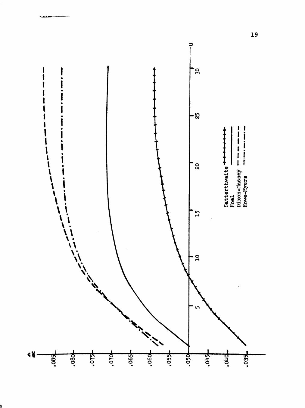
2. Probêújility of type-I error of procedures for n, = 2, n, = 2, and n^ = 1 as U - oo 19

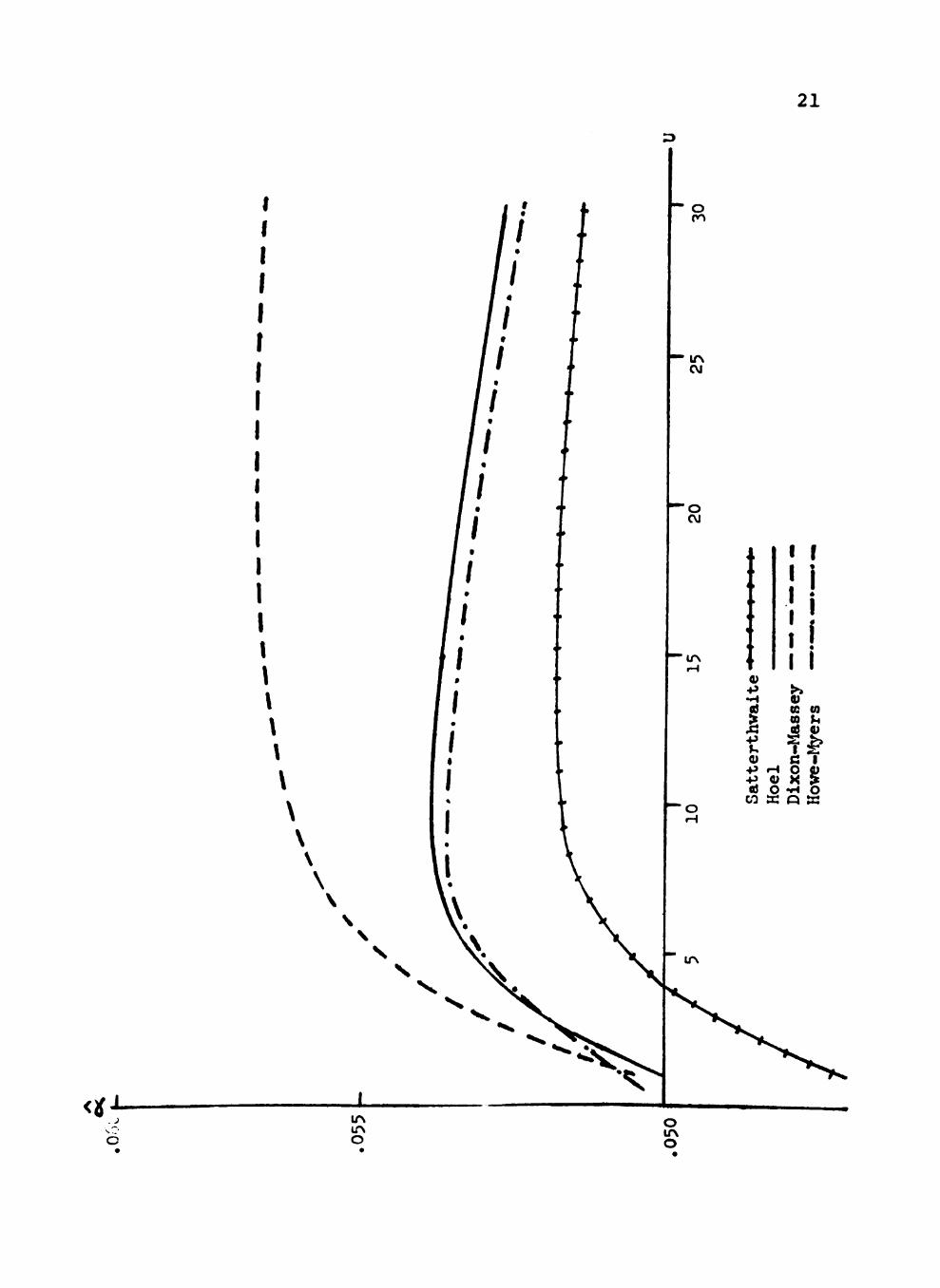
3. Probability of type-I error of procedures for n, = 6, n, = 6, and n^ = 1 as U -• <» 21

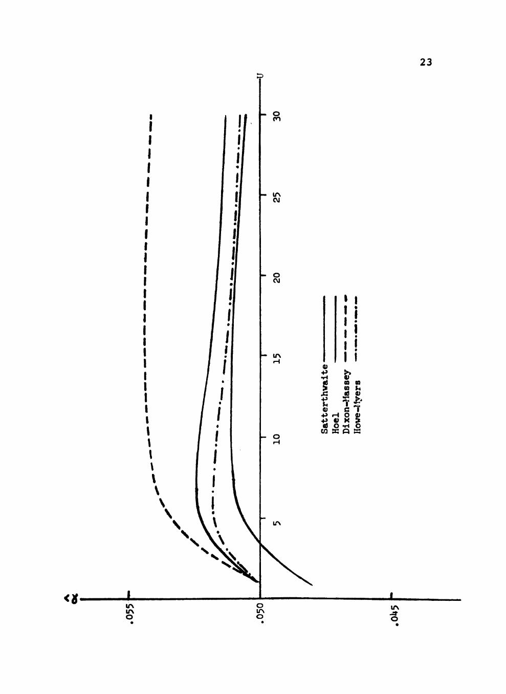
4. Probability of type-I error of procedures for n- = 18, n^ = 18, and n^ = 1 as U -> « 23

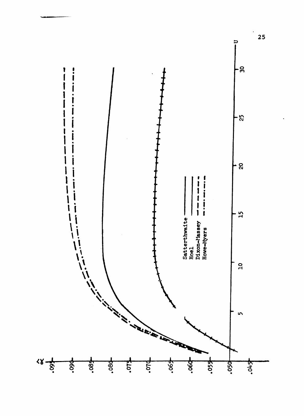
5. Probability of type-I error of procedures

for n, = 2, n^ = 6, and n^ = 1 as U -• » 25

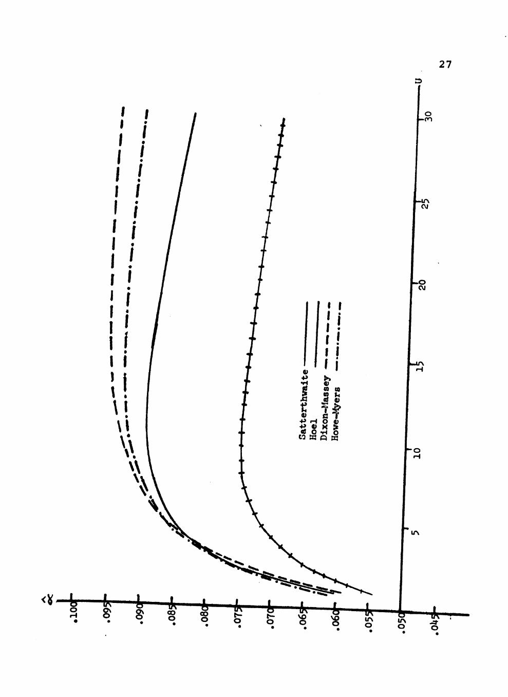
6. Probability of type-I error of procedures for n- = 2, n^ = 18, and n^ = 1 as U -> » 27

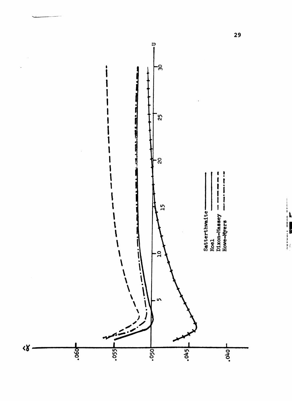
7. Probability of type-I error of procedures for n, = 6, n^ = 2, and n^ = 1 as U ^ » 29

8 Probability of type-I error of procedures for n, = 18, n^ = 2, and n^ = 1 as U -• « 31

Chapter 1

Introduction

In many statistical investigations, it is desiraúsle

to test hypotheses involving linear combinations of var-

iauice and covariance components for which an F-test of the

usual type does not exist^ A simple example is the Behren-

Fisher problem of comparing the means of two normal pop-

ulations with unknown and not necessarily equal variance

parauneters^ The following stuây considers one specific

case, testing the relation

6 3 = 6 ^ + 02

versus e^ > 6, + Ø^ (1)

where 6., i = 1*2,3 denotes variances from populations

which are assumed to be normally distributed^

Several methods have been suggested for testing hypo-

thesis (1)• Due to the approximate nature of these pro-

cedures, the value of the probability of the type-I error

is not exact^ Also, the implementation of many tests may

be considered impractical in various situations^

This study attempts to determine which of several

tests is "best" with respect to the closeness of the size

to the desired a and the simplicity of the procedure^

Chapter 2 is a survey of established guidelines. In Chap-

ter 3, five procedures are considered which have been pro-

posed by

1. Satterthwaite

2. Hoel

3. Dixon and Massey

4. Howe and Myers

5. Cochran.

The true size of the tests has been calculated, assuming a

desired confidence interval of 95 percent. The probability

of a type-I error is found by the following equation which

is derived in Chapter 3:

a = Pr(type-I error]

= ^o PIO ' fa[n3,f]-'^l"Î9(u)du

where Q = Central F statistic with n^ and n,+no 3 1 2

degrees of freedom,

F . ^. = the a upper percentage point of the a vn^ f r /

F-distribution with n^, the numerator degrees

of freedom and f, the estimated denominator

degrees of freedom

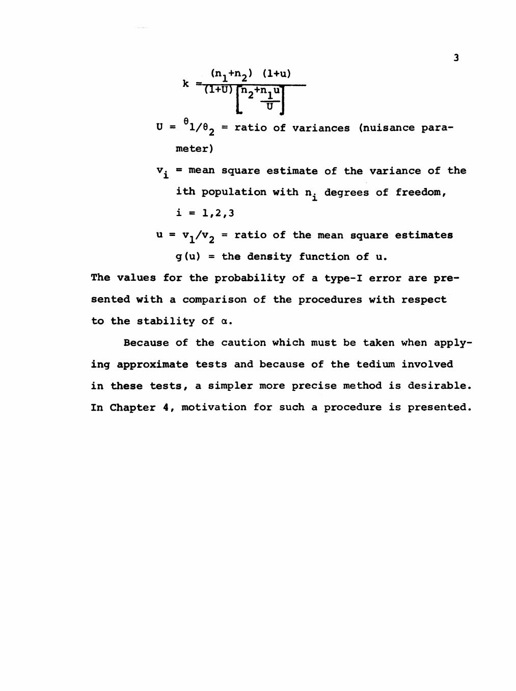
(n,+n,) (1+u) k =- ^ ^ TT+ y n^+ryi

u Q

U = l/Q^ ~ ratio of variances (nuisêuice para-

meter)

v^ = meéui square estimate of the variance of the

ith population with n. degrees of freedom,

i = 1,2,3

u = Vj /v = ratio of the mean square estimates

g(u) = the density function of u.

The values for the probability of a type-I error are pre-

sented with a comparison of the procedures with respect

to the stability of a.

Because of the caution which must be taken when apply-

ing approximate tests and because of the tedium involved

in these tests, a simpler more precise method is desirable.

In Chapter 4, motivation for such a procedure is presented.

Chapter 2

Earlier Comparative Studies

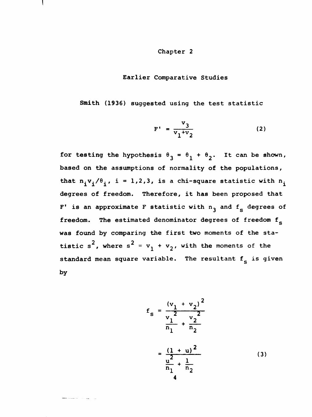
Smith (1936) suggested using the test statistic

F' = — T ^ (2) v^+V2

for testing the hypothesis Ø^ = 6. + Ø^. It cam be shown,

based on the assumptions of normality of the populations,

that n.v./e., i = 1,2,3, is a chi-square statistic with n.

degrees of freedom. Therefore, it has been proposed that

F' is an approximate F statistic with n^ and f degrees of

freedom. The estimated denominator degrees of freedom f

was found by comparing the first two moments of the sta-

2 2 tistic s , where s ~ ^i "*" 2' ^^^ ^ ® moments of the

stemdard mean square variable. The resultant f is given

by

(Vl ^ V2)'

^s 3 T-

n^ "2

. (1 + u ) ^

u . 1 (3)

n^ "" n^

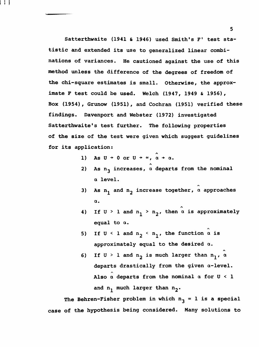
Satterthwaite (1941 & 1946) used Smith's F' test sta-

tistic and extended its use to generalized linear combi-

nations of variances. He cautioned against the use of this

method unless the difference of the degrees of freedom of

the chi-square estimates is small. Otherwise, the approx-

imate F test could be used. Welch (1947, 1949 & 1956),

Box (1954), Grunow (1951), and Cochran (1951) verified these

findings. Davenport and Webster (1972) investigated

Satterthwaite's test further. The following properties

of the size of the test were given which suggest guidelines

for its application:

1) AsU-^-OorU-*-*, a-^a.

2) As n^ increases, a departs from the nominal

a level.

3) As n, and n^ increase together, a approaches

a. A.

4) If U > 1 and n, > n^, then a is approximately

equal to a.

5) If U < 1 and n^ < n,, the function a is

approximately equal to the desired a.

6) If U > 1 and n, is much larger than n,, a

departs drastically from the given a-level.

Also a departs from the nominal a for U < 1

and n, much larger than n^*

The Behren-Fisher problem in which n^ = 1 is a special

case of the hypothesis being considered^ Many solutions to

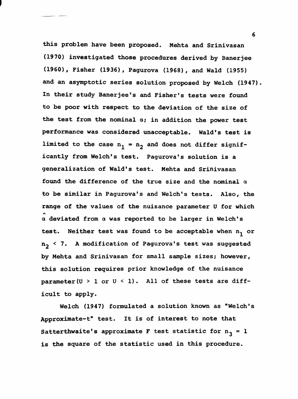
this problem have been proposed. Mehta and Srinivasan

(1970) investigated those procedures derived by Banerjee

(1960), Fisher (1936), Pagurova (1968), and Wald (1955)

and an asymptotic series solution proposed by Welch (1947)

In their study Banerjee's and Fisher's tests were found

to be poor with respect to the deviation of the size of

the test from the nominal a; in addition the power test

performcuice was considered unacceptable. Wald's test is

limited to the case n, = n, and does not differ signif-

icantly from Welch's test. Pagurova's solution is a

generalization of Wald's test. Mehta and Srinivasan

found the difference of the true size and the nominal a

to be similar in Pagurova's and Welch's tests. Also, the

range of the values of the nuisance parêuneter U for which A.

a deviated from a was reported to be larger in Welch's

test. Neither test was found to be acceptable when n. or

n^ < 7. A modification of Pagurova's test was suggested

by Mehta and Srinivasan for small sample sizes; however,

this solution requires prior knowledge of the nuisance

parameter(U > 1 or U < 1). All of these tests are diff-

icult to apply.

Welch (1947) formulated a solution known as "Welch's

Approximate-t" test. It is of interest to note that

Satterthwaite's approximate F test statistic for n^ = 1

is the square of the statistic used in this procedure.

Wang (1971) made a comparison of the approximate-t test

and the asymptotic series solution proposed by Welch for

the case a = .05 and a = .01. Deviation of the true

probability of a type-I error from a was found to be

slightly larger for the t-test. However, Wang (1971)

suggested the use of the approximate t-test due to the

ease of using the usual t tables and the fact that tables

of critical values for the asymptotic series solution are

available for only selected values of a. Preference for

"Welch's Approximate t" test was also supported by

Davenport éuid Webster (1974). Comparison was made of this

test to those results reported by Mehta and Srinivasan

(1970). It was shown that in general, Welch's approximate

test was better than Banerjee's and Fisher's, and less

stable than the others with respect to a. However, it was

suggested that ease in carrying out the t-test might be

ample justification for the use of "Welch's Approximate

t" test.

Chapter 3

Additional Comparative Studies of

Procedures for Testing ^2~^í^^2

An investigation of the stability of the size of

five procedures for testing the hypothesis given in

equation (1) has been conducted in order to present com-

parative guidelines for their use. Those procedures due

to Satterthwaite, Hoel, and Dixon and Massey, and Howe

and Myers' infinite series solution make use of Smith's

F' statistic, but suggest different methods for estimating

f, the denominator degrees of freedom. These estimates

are as follows:

Satterthwaite

f . 11±J1)1 (4)

n^ n^

Dixon and Massey

^D-M - , 2 Í5> rTjTT n^+l

8

Hoel

n^+2 ^2+2

Howe and Myers

^H-M " ^ " 2/(m(u) - 1)

where

00

kl u k+1 . k! 1 k+1 m(u) = 1 + 1 -^ ^ ^ •' + . ^» . £, k 1+u k n -• n (^ + j) n (^ + j)

j=l ^ j=l ^

2 l+^

Due to the reciprocal relation of the F distribution.

F <" l' 2> ^rj.r^) '

the value of the type-I error for specific values of U,

n, ,^2 is the same as for /U when the roles of n, and

n^ are interchanged. Therefore, without loss of general-

ity, values of a are presented for U > 1 only. Also,

calculations of a were restricted to the Behren-Fisher

problem (n^ = D • It is believed due to the nature of

the tests, that the effect of an increased value of n^

10

on a for tests considered in this chapter is the saroe as

that reported by Davenport and Webster (1971) for

Satterthwaite's procedure. Specifically, as n^ increases,

a departs from the nominal a level. Also the results re-

ported may be extended to the alternate hypotheses

83 < e^ + e^

êUld

63 e^ + 63

by applying usual techniques.

The method employed for finding the true probêúsility

of the type-I error of the approximate F tests is that

used by Davenport and Webster (1971). The size of the

test is given by

" = ^<^' * ^tnj.f])

where F , f\ ^^ ^^® ^^^ upper percentage point of the

F-distribution with n^ and f degrees of freedom. Due to /v

the âependency of f on u, a is a function of u, so that

PÍF' > F^, ^i) = í P(A|u)g(u)du (7) ain^»IJ Q

11

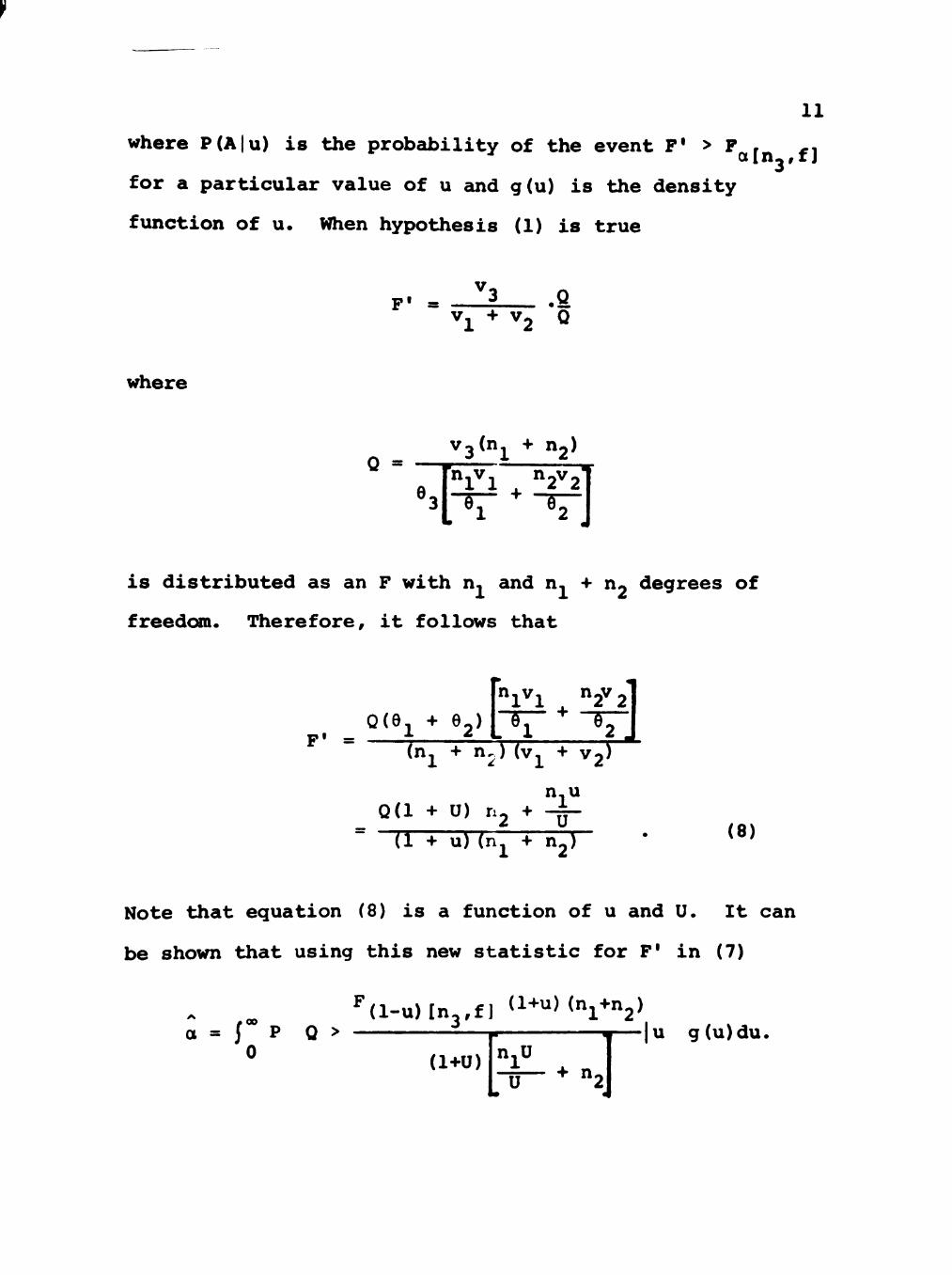
where P(A|u) is the probability of the event F' > F , ^, ain.^ij

for a particular value of u êmd g(u) is the density

function of u. When hypothesis (1) is true

F' = .Q v^ + V2 Q

where

Q = V3(n^ + nj)

e n^v^ n^v^

is distributed as an F with n^ and n, + n^ degrees of

freedom. Therefore, it follows that

F« =

K^l , "2 2 QiQ-^ + e ) ["T[~ T^

in^ + n7) iv^ + vj)

Q(l + U) n^ +

(1 + u) (Hj + n^)

n,u

(8)

Note that equation (8) is a function of u and U^ It can

be shown that using this new statistic for F' in (7)

. ^ ^(l-u)ln,,fj (l+u)(n^+n2) a = I P Q > -*

0 (1+U) nj U + n.

u g(u)âu^

12

This method of evaluating a was employed in computer pro-

grams, integration being accomplished by numerical

techniques^ The probabilities of the type-I error are

given in tables 1 - 4 for specific values of U, n^ and

nj with n- = l

V V

13

TABLE 1

Probability of a Type-I Error for Satterthwaite's Procedure at the Apparent 05 Level and n- = 1

V = ®i/e.

n. n. 16 30

2 2

6

6

2

18

18

2

6

2

6

18

2

18

0^0352

0^0469

0^0468

0^0471

0^0544

0^0544

0^0496

0.0373

0.0537

0.0441

0.0480

0.0627

0.0494

0.0498

0.0432

0.0621

0.0451

0.0501

0.0709

0.0480

0.0501

0.0564

0.0695

0.0498

0.0518

0.0743

0^0495

0^0502

0^0589

0^0675

0^0507

0^0514

0^0705

0^0499

0^0501

TABLE 2

Probability of a Type-I Error for Hoel's Procedure at the Apparent •OS Level and n^ = 1

V = ®i/e.

"1

2

2

6

6

2

18

18

n^

2

6

2

6

18

2

18

0.0503

0^0549

0^0548

0^0500

0^0607

0.0607

0.0500

0.0529

0.0637

0.0505

0.0509

0.0718

0.0535

0.0502

0.0595

0.0744

0.0501

0.0528

0.0830

0.0505

0.0504

16

0.0714

0.0833

0.0521

0.0536

0.0888

0.0501

0.0504

30

0.0716 0.0801

0.0521

0.0527

0.0839

0.0502

0.0503

14

TABLE 3

Probability of a Type-I Error for Dixon and Massey's Procedure at the Apparent .05 Level and n^ = 1

n. n. 16 20

2

2

6

6

2

18

18

2

6

2

6

18

2

18

0.0572

0.0562

0.0561

0.0505

0^0599

0^0599

O^OSOO

0.0601

0.0652

0.0519

0.0516

0.0710

0.0530

0.0502

0.0679

0.0768

0.0520

0.0540

0.0830

0.0504

0.0506

0.0847

0.0919

0.0556

0.0567

0.0954

0.0505

0.0509

0.0884 0.0932

0.0564

0.0567

0.0953

0.0508

0.0509

TABLE 4

Probability of a Type-I Error for Howe and Myers' Procedure at the Apparent .05 Level and n^ = 1

V = ®i/e.

"1

2

2

6

6

2

18

18

n^

2

6

2

6

18

2

18

0.0582

0.0563

0.0562

0.0503

0.0606

0.0606

0.0500

0.0611

0.0657

0.0515

0.0511

0.0717

0.0535

0.0501

0.0683

0.0771

0.0508

0.0528

0.0834

0.0506

0.0503

16

0.0821

0.0897

0.0522

0.0532

0.0931

0.0501

0.0503

20

0.0835

0.0890

0.0521

0.0524

0.0912

0.0502

0.0502

15

Values for the size of the tests due to Satter-

thwaite, Hoel, Dixon and Massey, and Howe and Myers sup-

ports the following relationships between the test

statistic parêuneters and the type-I error a:

1. As n^ = n^ increases in values, a

approaches a. /s

2. For U > 1 and small n^,a is unstable;

the discrepancy increases as n^ in-

creases.

3. For U < 1 and small n~, as n in-

creases the difference of a and a

increases.

4. When U > 1 and n.. small, a is close

to a, also a approaches the nominal

a as n., increases. i /\

5. When U < 1 and n, small, a is close to

a, and a approaches the nominal a as

xiy increases.

The preceding trend was fcund to be most exaggerated

in the procedure proposed by Djxon and Massey. Type-I

errors for Dixon and Massey's test are presented in Figure 1.

Satterthwaite's procedure is the most conservative

of the tests considered, as secn in figures 2 - 8 .

It can be shown that

fg i H "< S ' D-M'-

M í 1

3 u>

II

!-•

P 0)

G

4-

8 .

P) t3 Di

S P) (0 01 (D

»< -

co •0 n 0 o (D o. C ^{ (D

»-h O H{

< P> H{ H-0 c cn < 0) »-• c: (D (0

0 M>

»«í H' ^ .

»-• • •

*\3 H 0 tx P> cr H-M H-rt

^<

0 hh

rt »<

(D 1

H

(D ^

0 H

0 H í

o H-X 0 3

û % û i • 1

p

0 0 ' ^ ^ fH VO CVJ

l A l / \ O

O l A O

l/N

O

~ r' • —

UL

P F F F F F

> > > > > >

Q) 0)

C

4-

8 •

»0 H{ 0 o (D Oi c n (D (0

M» 0 •1

3 H'

II

> ^

3 lO

II

to ^

p) 3 Oi

3 CJ

II

^ H-

vQ •

N) • •

0 tr p) cr H-

H-rt

•< 0

r t ^< »0 (D 1

H

(D ^l

0 H{

0 H»

I I I I I

19

0)

•H aS

• p u 9)

& n m 09 u

4J H O 4) •p 0) X :» «5 O •H C CC X Q X

F F F F F F ^

\) [) \) \) [) \)

0) (0

G

+ 8

.

^ >1 0 O (D Oi c h (D (0

Mí 0 H

3 M

II

o\ ^

P lO

II

o\ ^

P) 9 Oi

3 OJ

II

^ H-

^ •

U> • •

»X3

0 CT 0) 0* H-

H-r t

*<

0 M»

r t

»0 (D 1

H

(D l-{ b{ 0 H

0 Mí

íl )l I Él )l »

O 00

21

<if-L

o

\

\

\

/

/

/

/

\r\ OJ

o OJ

i ,

( >

H 1 V +> •H ^ ^

.:: •p u u

1 r J 1 1 îí 1 1 >» 0) æ n tt >4 0) 0)

= é c i

O

F T

P) 01

C!

+ 8

.

»0 h 0 0 (D Oi (S H (D 01

M> 0 n 3

!-•

II

M 00 ^

P lO

II

!-• 00

^

0) :3 Oi

3 u>

•fl H-

vQ .

i ^ • •

»d H{ 0 tr & H-

H-rt

*< 0 M»

rt

•T3 (D 1

H

(D

h 0 h

0 M)

23

P M M P

(D 01

G

4-

8 .

»0 M 0 O (D Oi C M (D 01

M» O »1

3 !-•

II

lO ^

3 lO

II

<r> «

(D 3 Oi

3 CJ

II

• ^

H-vQ •

U l • •

0 cr & H-»-• H-rt

O M»

rt *< »0 (D 1

H

(D H

0 ^

0 M»

\ ;i M i k ll ll .

25

p) 01

G

4-

8 .

•0 h 0 o (D Oi

c H (D 01

M» 0 H

3 M

II

lO ^

3 lo

II

M æ ^

P) 3 Oi

3 u>

^ H-

vQ .

<T> • •

^ ^ o cr & H-!-• H-rt

*< O Mi

r t ^< »0 (D 1

H

(D H{ H{ 0 t-{

0 H\

27

i

;l !

Ut 01

G

4-

8 •

»0 h 0 0 (D Oi

c tt (D 01

Mî 0 H

3 M

II

m *

3 lO

II

lO ^

01 3 Oi

3 u>

II

•fl H-

vQ .

^ * t

•d

0 tr g-H-»-• H-

4 O M)

r t *< »0 (D 1

H

(D t{ h 0 H

0 Mí

29

<y

I i a> •p •H

s X t 0> •p •p tf co

H « O X

>» 0) n n n >4 ti o>

Ê* a 1 o o> X >

•H O Q X

vo O

U\ U\ O

O l A O

u\ J^ O

O

o

••

7

(U 01

G

4"

8 .

tJ h 0 o (D Oi

c H (D 01

M) 0 h

3 !-•

II

M 00

^

3 ro

11

lO

(U 3 Oi

3 o>

II

^ H-vQ .

00 * .

t{ 0 cr & H^

H^ rt *<

O M>

r t »<

(D i

H

(D K

0 H

O M>

, '1 , 1

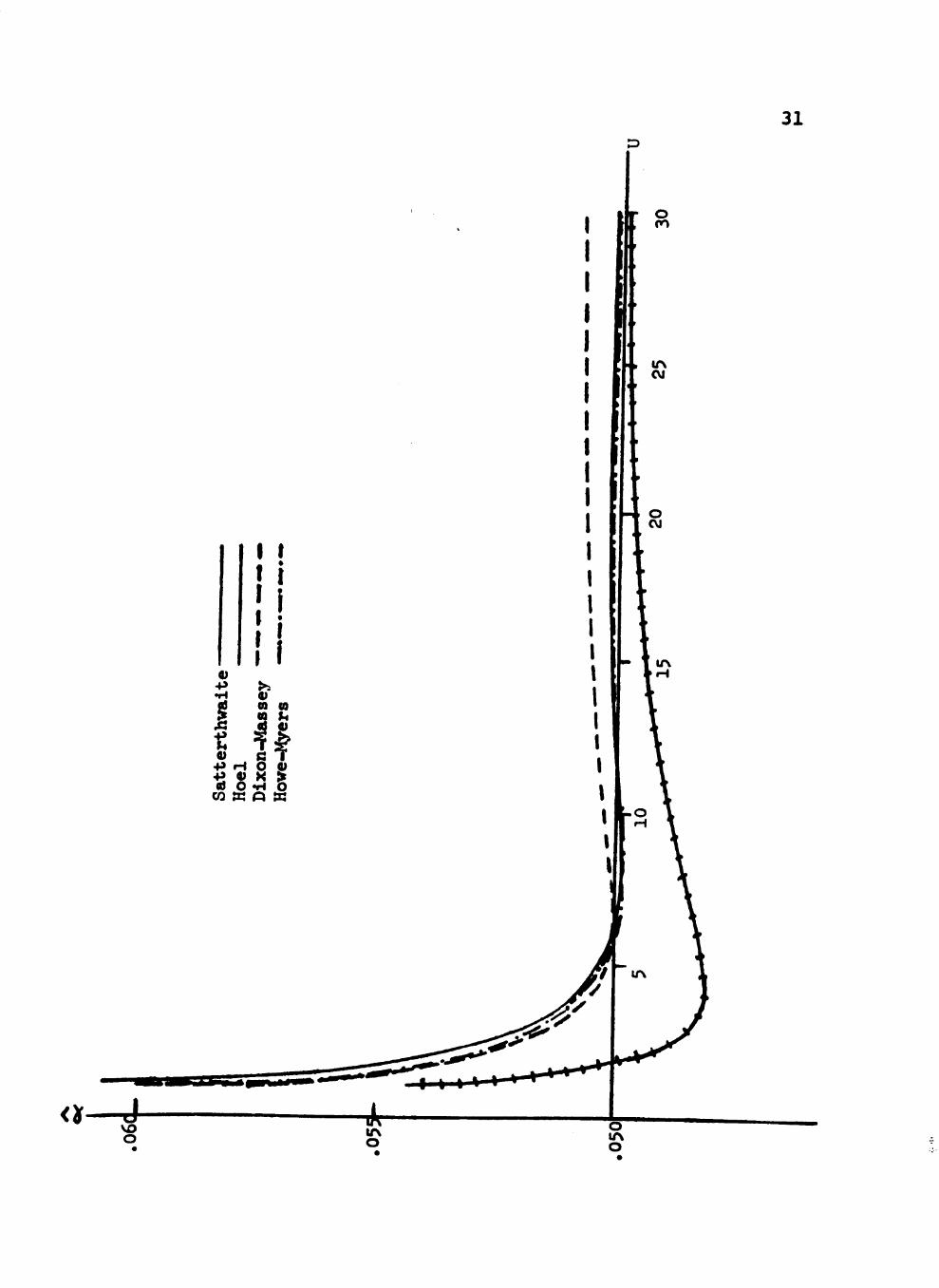
31

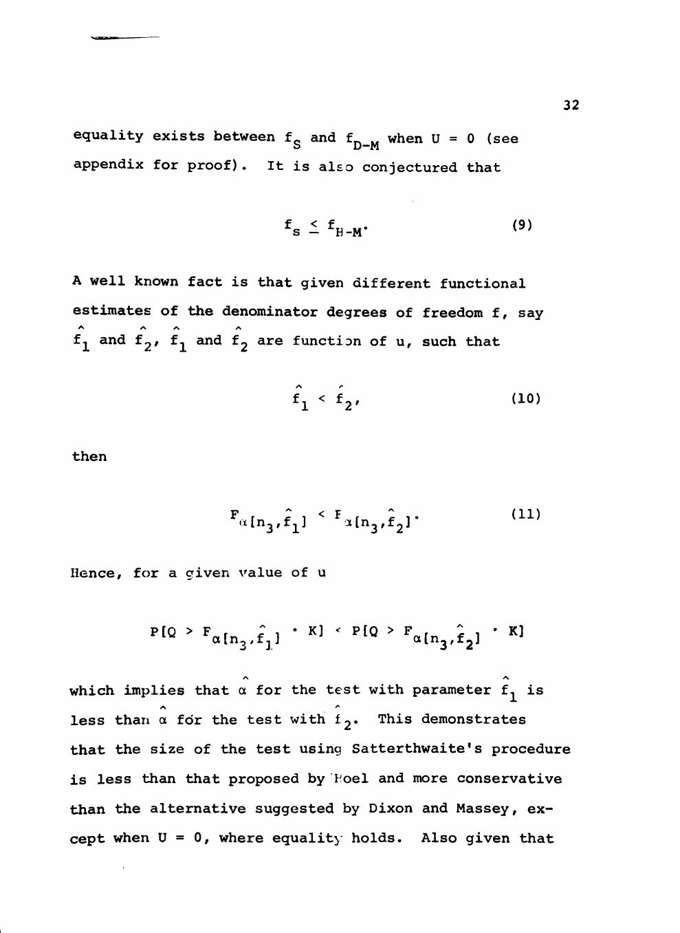
32

equality exists between f. and f when U = 0 (see o D—M

appendix for proof). It is also conjectured that

s i h-M- <9)

A well known fact is that given different functional

estimates of the denominator degrees of freedom f, say

fj and f / fj and f are functÍDn of u, such that

^l < ^2' ^^^^

then

F r í 1 < F r 2 i. (H)

l i e n c e , f o r a g i v e n v a l u e of u

P[Q > F r r , • K] < P[Q > F , 2 1 • ^^ ^ [ n ^ ^ f j ] ' ^ a í n ^ ^ f ^ ]

K]

which implies that a for the test with parameter f, is

less than a fdr the test with í^. This demonstrates

that the size of the test using Satterthwaite's procedure

is less than that proposed by Hoel and more conservative

than the alternative suggested by Dixon and Massey, ex-

cept when U = 0, where equalit - holds. Also given that

33

inequality (9 ) holds, the size of Satterthwaites test is

also less than or equal to the size of the procedure

suggested by Howe and Myers.

For Satterthwaite's procedure a is generally close

to the desired a level and the range of values of the

nuisance parameter for which there is large deviation

from the nominal a is less in most cases. However, the

case n. = 18, n^ = 2, U > 1 merits closer inspection.

Under these conditions the behavior of a due to Hoel's

test is better than Satterthwaite's (see figure 8). It

is therefore suspected that given U > 1, small n^ and

large n, or U < 1, small n.. and large n^t Hoel's pro-

cedure should be used.

The "Cochran t-test" is an asymptotically normal

solution of the Behren - Fisher problem. This pro-

cedure applies the test statistic

"'l" ""^ (12)

where X. is the arithmetic mean of the ith population,

i = 1,2. The critical point C is given by

V,t + V t^ c = ^ ^ ^ ^ (13) ^ V^ + V^ ^ '

where t. is the 100 (l-a/2) percentage point of the

34

t-distribution with n. degrees of freedom. /

Specific values of a resulting frora Satterthwaite's

test were evaluated for comparison with the size of the

"Cochran t-test" reported by Lauer and Han (1971). These

are presented in table 5 along with the maximum deviation

of a from a for each test over the given four values of U.

It is observed that Cochran's test is more conservative

than Satterthwaite's.

It is believed that further investigation is needed

in order to present specific guidelines for determining

when Cochran's t-test should be applied. However, it

appears that when n^ is much larger than n and U is

assumed to be greater than one, Cochran's test is "best"

with respect to the closeness of a to the desired a. For

all other cases, Satterthwaite's test appears better than

Cochran's. Therefore, if U < 1 or no prior knowledge of

its value is known, Satterthwaite's procedure should be

employed.

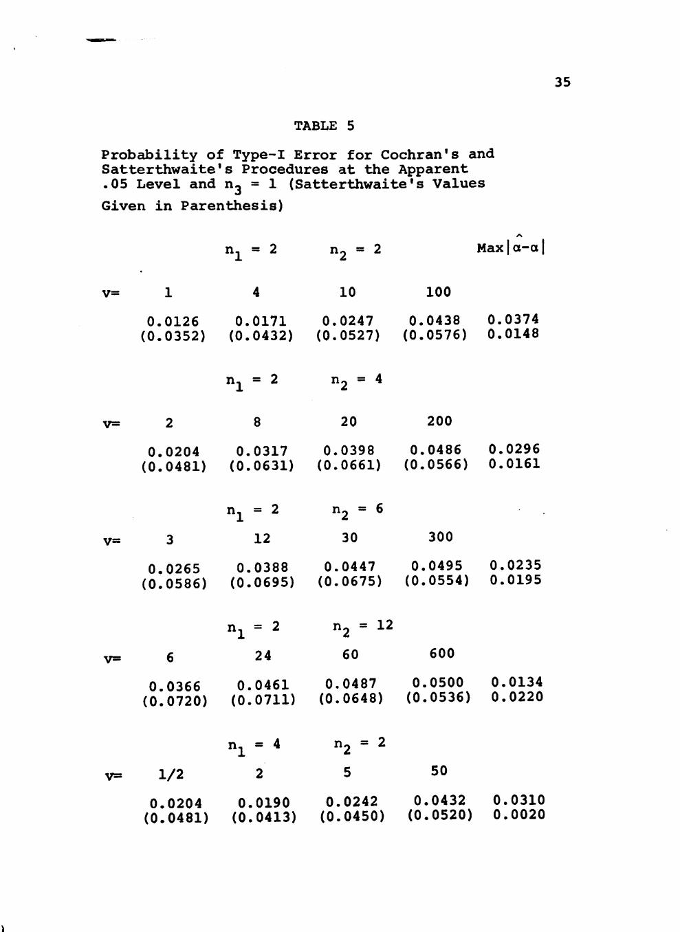
TABLE 5

Probability of Type-I Error for Cochran's and Satterthwaite's Procedures at the Apparent .05 Level and n^ = 1 (Satterthwaite's Values

Given in Parenthesis)

35

n, = 2 n^ = 2 Max a-a

v= 10 100

0.0126 (0.0352)

0.0171 (0.0432)

0.0247 (0.0527)

0.0438 (0.0576)

0.0374 0.0148

n, = 2 n^ = 4

v= 8 20 200

v=

v=

v=

0.0204 (0.0481)

3

0.0265 (0.0586)

6

0.0366 (0.0720)

1/2

0.0204 (0.0481)

0.0317 (0.0631)

n, = 2

12

0.0388 (0.0695)

n, = 2

24

0.0461 (0.0711)

n, = 4

2

0.0190 (0.0413)

0.0398 (0.0661)

n^ = 6

30

0.0447 (0.0675)

n^ = 12

60

0.0487 (0.0648)

n^ = 2

5

0.0242 (0.0450)

0.0486 (0.0566)

300

0.0495 (0.0554)

600

0.0500 (0.0536)

50

0.0432 (0.0520)

0.0296 0.0161

0.0235 0.0195

0.0134 0.0220

0.0310 0.0020

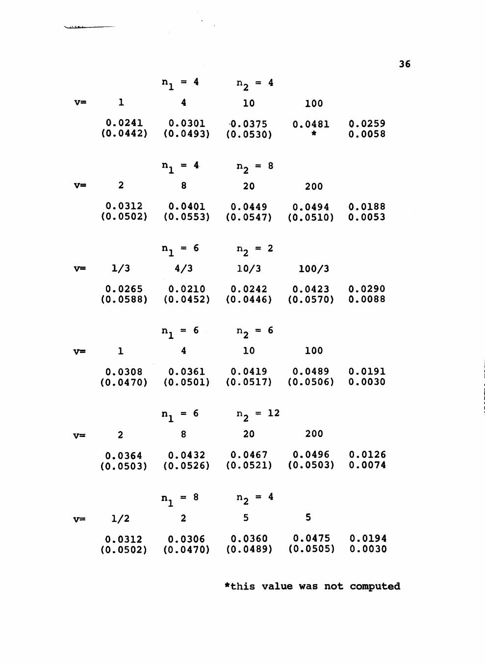
36

v=

v=

v=

v=

v=

v=

1

0.0241 (0.0442)

2

0.0312 (0.0502)

1/3

0.0265 (0.0588)

1

0.0308 (0.0470)

2

0.0364 (0.0503)

1/2

0.0312 (0.0502)

n, = 4

4

0.0301 (0.0493)

n3_ = 4

8

0.0401 (0.0553)

n, = 6

4/3

0.0210 (0.0452)

n^ = 6

4

0.0361 (0.0501)

n.. = 6

8

0.0432 (0.0526)

2

0.0306 (0.0470)

n^ = 4

10

0.0375 (0.0530)

n^ = 8

20

0.0449 (0.0547)

n^ = 2

10/3

0.0242 (0.0446)

n^ = 6

10

0.0419 (0.0517)

^2 = 2

20

0.0467 (0.0521)

n^ = 4

5

0.0360 (0.0489)

100

0.0481 *

200

0.0494 (0.0510)

100/3

0.0423 (0.0570)

100

0.0489 (0.0506)

200

0.0496 (0.0503)

5

0.0475 (0.0505)

0.0259 0.0058

0.0188 0.0053

0.0290 0.0088

0.0191 0.0030

0.0126 0.0074

0.0194 0.0030

*this value was not computed

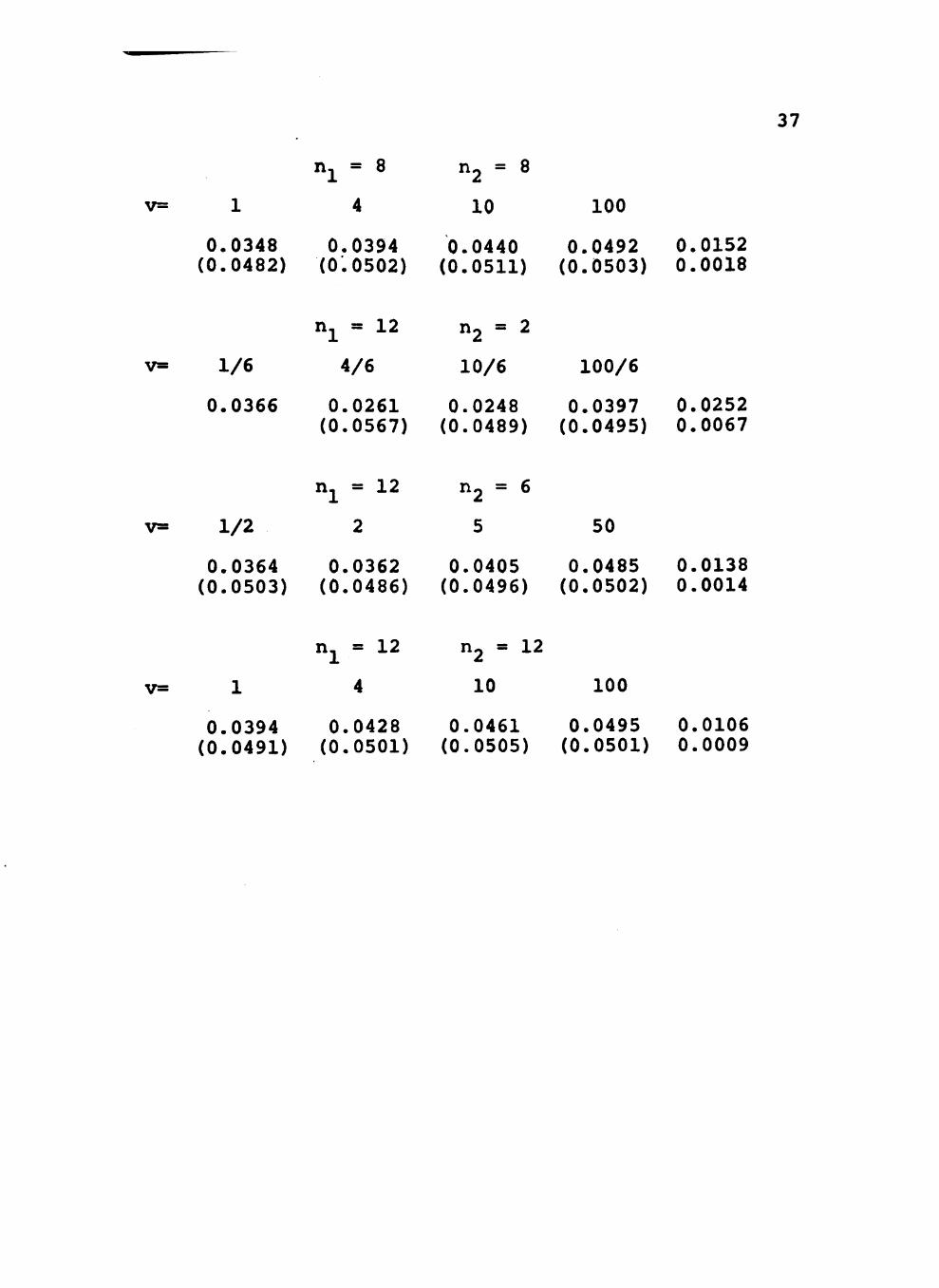
37

v=

v=

v=

v=

1

0.0348 (0.0482)

1/6

0.0366

1/2

0.0364 (0.0503)

1

0.0394 (0.0491)

n^ = Q

4

0.0394 (0.0502)

n^ = 12

4/6

0.0261 (0.0567)

n^ = 12

2

0.0362 (0.0486)

n^ = 12

4

0.0428 (0.0501)

n^ = 8

10

0.0440 (0.0511)

n^ = 2

10/6

0.0248 (0.0489)

n^ = 6

5

0.0405 (0.0496)

n^ = 12

10

0.0461 (0.0505)

100

0.0492 (0.0503)

100/6

0.0397 (0.0495)

50

0.0485 (0.0502)

100

0.0495 (0.0501)

0.0152 0.0018

0.0252 0.0067

0.0138 0.0014

0.0106 0.0009

Chapter 4

Motivation for the Development of

an Improved Procedure

Available tests for evaluating hypothesis (1) often

involve approximate procedures. Therefore, a simple, con-

cise, approximate solution to the problem which is as good

as, if not better than existing ones is needed. A search

for such a procedure has been conducted. At present this

problem is unresolved; however, motivation for the develop-

ment of an improved test is presented.

As previously shown, the true probability of a type-

1 error a is given by

a = Jo P(Q > F„(n,,f)' k]g(u)du.

Note that Q is a central F statistic with n^ and n, + n^

degrees of freedom. By letting f = n^ + n^ the percentage

point is now F , „ 4.« \ ^^^ i^ from the same distribution

as Q and no longer a function of u. Let h = h(u;n,^n^)

be some function such that h is approximately equal to k,

hence k/h = 1. The probability of type-I error is

38

39

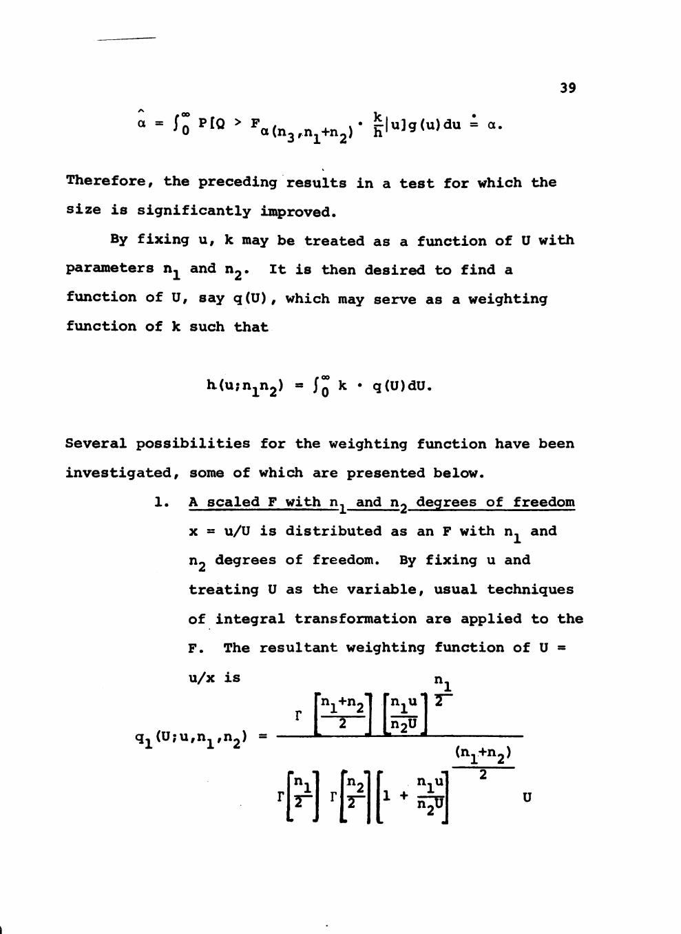
a = ÍÂ PlQ > F , ,• ^|u]q(u)du = a. ''O ^^ aín^^n^^+n^) h' '' ^ '

Therefore, the preceding results in a test for which the

size is significantly improved.

By fixing u, k may be treated as a function of U with

parameters n ^ and n^. It is then desired to find a

function of U, say q(U), which may serve as a weighting

function of k such that

KCu^nj^n^) = ÍQ k • q(U)dU.

Several possibilities for the weighting function have been

investigated, some of which are presented below.

1• A scaled F with n, and n^ degrees of freedom

X = u/U is distributed as an F with n^ and

n^ degrees of freedom. By fixing u and

treating U as the variable, usual techniques

of integral transformation are applied to the

F. The resultant weighting function of U =

u/x is

qj^(U;u,nj^,n2) = ' pp\ [ ] 3 -

Mflh^ (n +n )

U

40

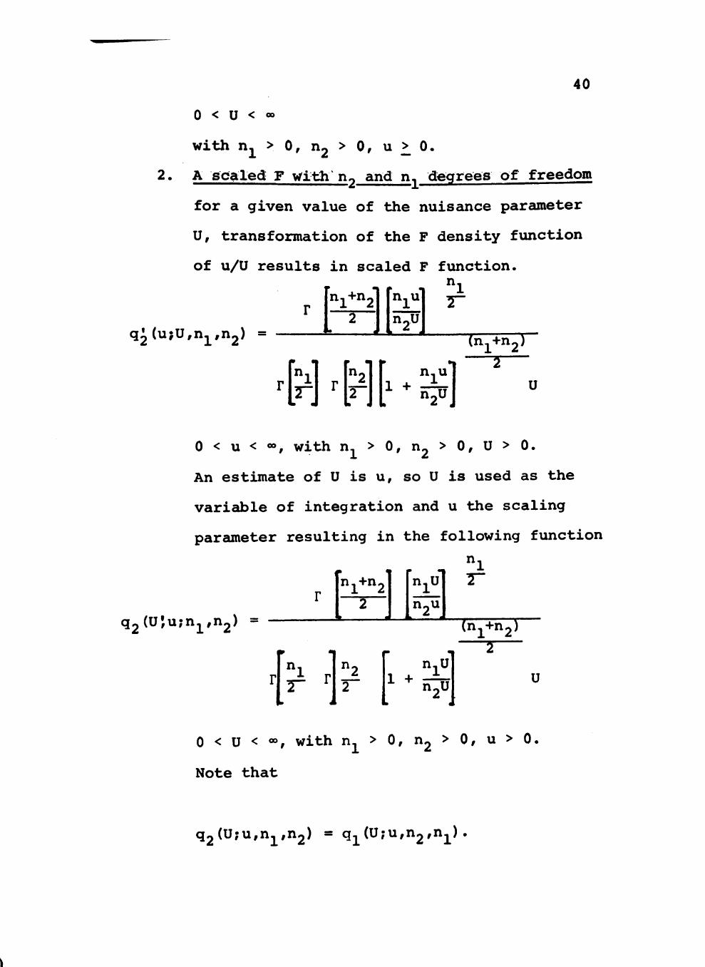
0 < u < »

with n, > 0, n, > 0, u > 0.

2. A scaled F with n^ and n ^ degrees of freedom

for a given value of the nuisance parameter

U, transformation of the F density function

of u/U results in scaled F function. n.

q^(u?U,nj^,n2) =

H'Mh l (n^+n^)

U

0 < u < «>, with n, > 0 , n 2 > 0 , U > 0 .

An estimate of U is u, so U is used as the

varicúsle of integration and u the scaling

parameter resulting in the following function

q^^Uîu^n^^^n^) =

n^+n^ n U

n^u

^l 7"

[^l 1^2 r l"

(n^+n^)

2

u

0 < U < ~, with n ^ > 0 , n 2 > 0 , u > 0 .

Note that

q^^U^u^n^^n^) = q ^ (U^u^n^fnj^) .

41

3. A chi-square with u degrees of freedom

Since u is an estimate of U and Ely] = y

where y is distributed chi-square with y

degrees of freedom, it seems reasonable to

let u be the degrees of freedom of the chi-

square prior function.

4. Chi-square with n^u/^n^-^) degrees of freedom

u/U is distributed F, . , therefore (nj n )

E[u/U] = ^2/(^2-2) which implies E[u] =

^2^/(^2-2) and U ^n^Eíuj/^n^-^). Therefore

n^u/^n^-^) is chosen as the degrees of free-

dom of the chi-square function.

5. Normal with mean u aná arbitrary variance

All weighting functions considered, when applied as pre-

viously suggested, resulted in unstable values of a; hence,

did not improve the approximate test.

It is suggested that the technique of curve fitting

may be applied to obtain a function h^u^n^^n^). Also an

investigation of the denominator degrees of freedom of the

F' statistic might be of value. A new procedure has been

evaluated for which the estimated denominator degrees of

freedom f is given by

f = minlfjj^^^n^^+n^].

42

The probability of a type-I error is more conservative

than that which resxilts from Howe and Myers' infinite

series solution and greater than Satterthwaites. This

technique, however, does not result in an improved test.

Chapter 5

Conclusions and Recomendations

Procedures for testing the hypothesis 63 = Ôi + ^2

are approximate and therefore the value of the type-I

error is not exact. Instability of the size of the test

is related to the parameters n, n^^n^ and U = ^-t/^o ^"^

the chosen procedure. Consequently, the size of the sample

taken from the population should be carefully determined

with consideration given to the relation of 6, to B^,

when it is known. Also the test should be chosen with

respect to the available degrees of freedom and the value

of the nuisance pareuneter.

Given no prior knowledge of the value of the nuisance

parameter, large, equal sample sizes should be taken when-

ever possible. Satterthwaite's relatively simplistic pro-

cedure may then be applied with confidence due to the sta-

bility of the test when the degrees of freedom are large

and equal.

When the situation is such that only small equal

sample sizes are available, Mehta and Srinivasan's mod-

ification of Pagurova's procedure may be used. However

the procedure involves knowledge as to whether U is great-

er thcui or less than one. Howe and Myers (1970) have 43

44

suggested euiother procedure which is good when n. and n^

cure small and equal. For the case being considered the

test criterion C(v,, v^, a) déveloped by Howe and Myers

is such that, given the null hypothesis is true.

Prlv^ > C{V^,V2,OL)] = a.

C(v,,V2,cx) is a series expansion developed by successive

approximations and involves the upper lOOa percentage

point of the gamma distribution with parameters a = 3/2

and 3 = 1 . This procedure's complexity makes it imprac-

tical in m£uiy situations and the technique involved is

beyond the intended extent of this text; therefore, the

equation for C(v, v yOi) is not included here.

If the relationship of 6. cuid 6 is known, then a

larger scunple should be taken from the population with

greatest variance. Then Hoel's test may be applied with

confidence. If however, it is necessary for a much

larger sample size to be taken from the population with

least variability, application of Cochran's test is

suggested.

REFERENCES

Banerjee, S.K. (1960). "Approximate Confidence Interval

for Linear Functions of Means of k Populations When

the Population Variances are Not Equal," gankhva 22,

357-8.

Box, G.E.P. (1954). "Some Theorems on Quadradic Forms

Applied in the Study of Analysis of VaricUice Problems,

I. Effect of Inequality of Variance in the One-Way

Classification," Ann. Math. Sta^^. 25, 290-302.

Cochran, W.G. (1951). "Testing a Linear Relation Among

Variances," Biometrics 7, 17-32.

Davenport, James M., and Webster, J.T., (1972). "Type-I

Error and Power of the Test Involving a Satter-

thwaite's Approximate F Statistic," Techometrics 14,

555-69.

Fisher, R.A. (1936). "The Fidueial Argument in Statistical

Inference," Ann• Euaei 6, 62-71.

Grunow, D.G.C. "Test for the Significance of the

Difference between Means in Two Normal Populations

having Unequal Variances." Bíf metrik 38, 252-256.

Howe, R.B. and Myers, R.H. (1970) , "An Alternative to

Satterthwaite's Test Involving Positive Linear

Combinations of Variance Components." J. Am. Stat.

Assn. 65, 404-412.

Lauer, G.N. (1971), "Power of Cochran's Test in Behren-

Fisher Problems." Unpublished Ph.D. Thesis, Ames,

lowa, Library, lowa State University of Science

and Technology.

45

46

Mehta, J.S., and Sriniuasan, R. (1970). "On the Behrens-

Fisher Problem." Biometr: |c 57, 649-55.

Pagurova, V.I. (1968), "Tests of Comparison of Mean Values

Based on Two Normal Samples." (Russian.) No. 5 Com-

puting Center of the Academy of Sciences of the

U.S.S.R. Moscow.

Satterthwaite, F.E. (1941). "Synthesis of Variance."

Psvchometril^^ 6, 309-16.

Satterthwaite, F.E. (1946). "An Approximate Distribution

of Estimates of Variance Components." Biometrics 2,

110-4.

Smith, H.F. (1936), "The Problem of Comparing the Results

of Two Experiments with Unequal Errors." Journal of

the Cottngil fgr Sgienti^jc and n^ugtrifll Researgh 9, 211-2.

Wald, A. (1955), "Testing for Difference Between the Means

of Two Normal Populations with Unknown Standard

Deviations." Selected Papers in Stat^stic s and

Prf^bahilítY by A. Wald, New York: McGraw-Hill.

Wang, Y.Y. (1971). "Probabilities of the Type-I Errors

of the Welch Tests for the Behrens-Fisher Problem."

.T. Am- Stat. Assn. 66, 605-8.

Welch, B.L. (1947). "The Generalization of Students'

Problem when Several Different Population Variances

are Involved." Biometrika 34, 28-35.

Welch, B.L. (1949). "Further Notes on Mrs. Aspin's Tables

and on Certain Approximations to the Tabled Function."

Biometrika 36, 293-6.

Welch, B.L. (1956). "On Linear Combinations of Several

Variances." J, Amer. Stat. ^fg§^9f 51, 132-48.

APPENDIX: THEOREMS AND PROOFS

48

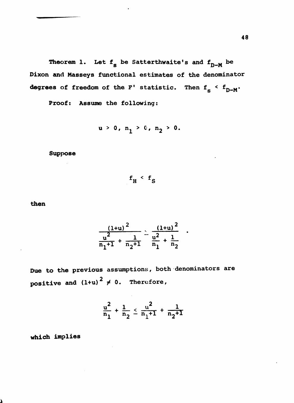
Theorem 1. Let f be Satterthwaite' s aná f^ „ be S D—M

Dixon and Masseys functional estimates of the denominator

degrees of freedom of the F' statistic. Then f < f -M* Proof: Assiune the following:

u > 0, n- > 0, n^ > 0.

Suppose

^H^ ^S

then

(1+u)^ 2 1 -

n , + l ' n^+l

(1+u)^

n^ "2

Due to the previous assumptions, both denominators are

positive and (1+u)^ j^ 0. Therefore,

HÍ + i- < - H L + 1 n, n^ — n,+l n^+l

which implies

49

u2 1 n^(nj^+1) •*• njnipT) - ^'

But thi8 i8 i]npo88Íble.

Hence, f^ < f^_^.

Theorem 2. Let f be Satterthwaite's and f„ Hoel's

functional estimates of the denominator degrees of free-

dom of the F* statistic. Then f < f„. S — H

Proof: Assume the following

u > 0, n, > 0 and n^ > 0.

Suppo8e

^H < ^S

then

(1+u)^ . (1-m)^ . 2

!íl + i- ^ + ^ n, n^ nj +2 n^+^

Given the preceding assunptions the following steps are

obtained U8ing ordinary algebraic techniques.

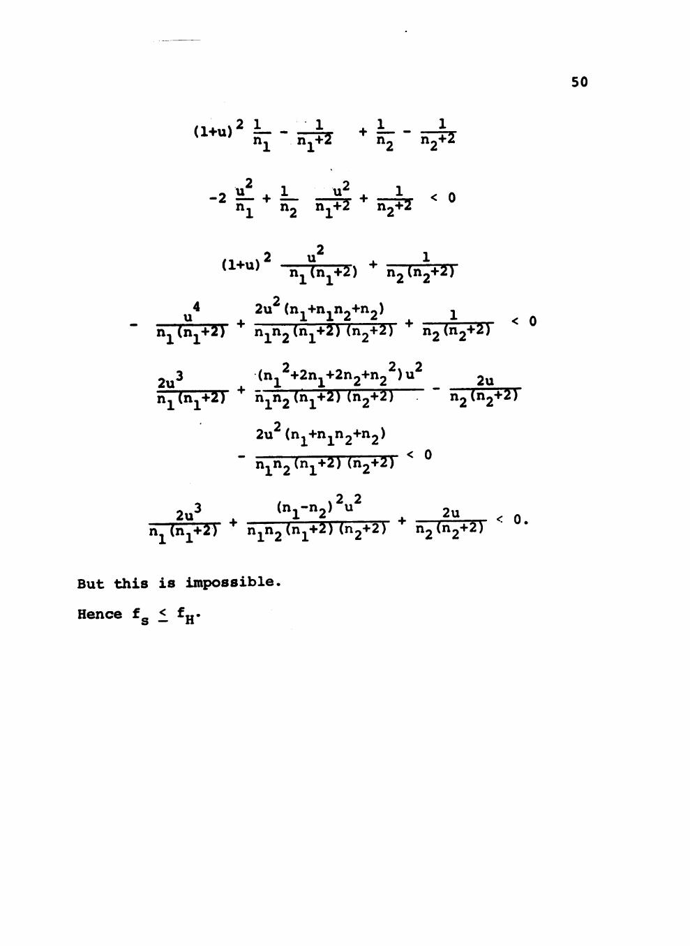
50

< 0

<^*«>'^-n^ *k-4^

-2^ + í- —4 + —K < 0 " l "^2 "^T*^ ^2+2

2 2 j <^*''> nJn^+2) * n j (n^+^)

^4 2u (nj +nj n^+n ) j n ^TnJjTÎT "*" nj^n^^nj^+î) (n^+Z) **" n^ín^+^)

25i3 (n^^+2n^+2n2+n2^)u^ 2u îrjTK~+2T "*" h^n^in^+^) (^2+2) " ' n^ín^+Z)

2u (n^+n^n^+n^)

nj^n^ínj^+^) (n^+Z) ^ ^

2^3 ( n ^ - n 2 ) V ^u . ^ n^(n^+Í) * n^n2(n^+2)(n2+2) * n^ín^+^) "*

But this is impo88Íble

Hence fg — ^H*