COASTAL ENGINEERING

Coastal Engineering 3 1 (1997) 163- 198

Comparisons between sediment transport models and observations made in wave and current flows

above plane beds

A.G. Davies aV*, J.S. Ribberink bP1, A. Temperville ‘, J.A. Zyserman d

a School of Ocean Sciences, Universiry oj’wnles (Bangor), Marine Science Laborutories, Menui Bridge.

Gwynedd, LL59 SEY, UK

b De@ Hydraulics, P.O. Box 152. NL-8300 AD Emmeloord, The Netherlands

’ Institut de M&unique de Grenoble. B.P. 53, F-38041 Grenoble. France

d Danish Hydraulic Instirute. Agern Alle 5, DK-2970 Horsholm, Denmark

Received 15 March 1996; accepted 20 December 1996

Abstract

As a part of the MAST2 GS-M Coastal Morphodynamics project, the predictions of four sediment transport models have been compared with detailed laboratory data sets obtained in the bottom boundary layer beneath regular waves, asymmetrical waves, and regular waves superim- posed co-linearly on a current. Each data set was obtained in plane bed, sheet flow, conditions and each of the four untuned numerical models has provided a one-dimensional vertical (lDVj, time-varying, representation of the various experimental situations. Comparisons have been made between the model predictions and measurements of both time-dependent sediment concentration, and also wave-averaged horizontal velocity and concentration. For the asymmetrical waves and for the combined wave-current flows, comparisons have been made with vertical profiles of the cycle-averaged sediment flux, and also with the vertically-integrated net sediment transport rate. Each of the turbulence diffusion models gives an accurate estimate of the net transport rate (invariably well within a factor of 2 of the measured value). In contrast, none of the models provides a good detailed description of the time-dependent suspended sediment concentration, due mainly to the inability of conventional turbulence diffusion schemes to represent the entrainment of sediment into suspension by convective events at flow reversal. However, in the cases considered here, this has not seriously affected the model predictions of the net sediment flux, due

’ Corresponding author. ’ Present address: University of Twente, Faculty Technology and Management, Department of Civil

Engineering, P.O. Box 217, Enschede, The Netherlands.

0378.3839/97/$17.00 Copyright 0 1997 Elsevier Science B.V. All rights reserved.

PII SO378-3839(97)00005-7

164 A.G. Davies et al./Coustal Engineering 31 (1997) 163-198

to the dominance of the near-bed transport. The comparisons in this paper are aimed not only at testing the predictive capability of existing sediment transport modelling schemes, but also at highlighting some of their deficiencies.

Keywords: Comparison of models; Current flows; Plane beds; Sediment transport models; Transport models;

Wave flows

1. Introduction

The accurate prediction of net sediment transport rates in coastal areas presents a

major challenge to engineers and oceanographers concerned with such problems as onshore-offshore sediment transport and long-term morphological change. It is not surprising, therefore, that numerous models of sediment transport by waves and currents

have been proposed, ranging from simple quasi-steady models based on Bagnold’s energetic principles to complex numerical models involving higher-order turbulence closure schemes. Only recently have sufficiently detailed near-bed velocity and sediment

concentration data become available to test not only the overall predictions of net sediment transport made by different modelling schemes but also, very importantly, the accuracy with which these schemes represent detailed boundary layer processes in reversing oscillatory flows.

Following the instructive intercomparison of hydrodynamical models of wave-cur- rent interaction in the bottom boundary layer carried out in the MAST1 G6-M Coastal Morphodynamics project (see Soulsby et al., 19931, it was decided to carry out a comparison of models of sediment transport in wave and current flow in the subsequent MAST2 G8-M project. This paper presents the results of the intercomparison, and assesses not only the predictive capabilities of existing modelling schemes, but also their potentially serious limitations.

The data used in the present comparisons were obtained during the MAST G6-M and G8-M projects by Ribberink and Al-Salem (1992, 1994, 1995) for regular symmetrical and asymmetrical waves, and by Katopodi et al. (1994a,b) for combined wave and current flows. The experiments were carried out in the Large Oscillating Water Tunnel (LOWT) at Delft Hydraulics, The Netherlands. All of the data were obtained in wave-dominated conditions above plane sand beds, corresponding to very vigorous conditions in nature.

Within the G8-M group, four existing numerical models were made available for the present study. Each of these models was of the conventional turbulence diffusion type and was run, for the sheet flow conditions of present interest, in a one-dimensional vertical (lDV> manner. The detailed temporal and vertical resolution in the LOWT data allowed a range of comparisons to be made between the observations and the model predictions, from time-dependent sediment concentrations during the wave cycle, to the measured net (i.e. temporally and vertically averaged) sediment transport rates.

It is well known that hydrodynamical processes in the wave and current bottom boundary layer are highly nonlinear (see, e.g., Soulsby et al., 1993). However, nonlin- earity is even more pronounced in relation to sediment transport processes, due to the additional constraints of the threshold condition for sediment motion and of the

A.G. Dooies et al./ Coastul Engineering 31 (1997) 163-198 165

nonlinear relationship between the bed shear stress and the sediment pick-up rate. It is

therefore surprising that simple, quasi-steady, representations of sediment transport in unsteady flow (e.g., Bailard, 1981) have achieved such wide acceptance. This, however, is due primarily to the simplicity offered by these methods in terms of practical application, rather than to their validity in representing physical processes correctly. For example, the neglect in such models of a description of the height- and time-varying nature of the velocity and sediment concentration fields means that they cannot represent either detailed suspension effects in unsteady flow, or the vertical structure of the net sediment flux. This objection extends also to time-averaged (“current-related”) ap- proaches for the prediction of the suspended sediment transport rate adopted by, for

example, Glenn and Grant (1987) and van Rijn (1991), which neglect the potentially

important “wave-related” contribution to the net transport. This is not to say that more

complicated turbulence modelling schemes, involving time-variation in velocity and concentration, necessarily represent oscillatory boundary layer processes correctly. It will be shown later that our present incomplete understanding of momentum transfer, and of the associated sediment pick-up, in reversing oscillatory flows imposes poten- tially severe limitations on all existing predictive methods.

The “wave-related” contribution to the suspended sediment flux, which is poten- tially important for grains confined to the oscillatory boundary layer, arises from unsteadiness both in the sediment entrainment rate from the bed and in the vertical diffusivity of sediment (see, e.g., Fredsoe, 1993; Davies, 1995). At a particular height (2) in the wave boundary layer, the phase relationship between the sediment concentra- tion c( z,t> and horizontal velocity U( z,t) (t = time) significantly influences the wave- related contribution in a way which may either enhance or inhibit the net flux and which may, in some circumstances, dominate the suspended sediment transport. This has been demonstrated in experiments carried out in sheet flow conditions by Ribberink and Al-Salem (1992, 1995) for asymmetrical waves, who found that unsteadiness in u and c produced an “onshore” net transport of sediment close to the bed, and an “offshore” transport above this in the outer suspension layer. The importance of the “wave-related” contribution has been demonstrated in the laboratory for combined wave-current flows by Murray et al. (1991) for regular waves above both rippled and plane beds, by Villaret and Perrier (1992) for rippled beds, and by van Rijn et al. (1993) for irregular waves above rippled beds. In each of these studies, the wave-related transport was directed against the current direction. Field observations showing the variability of wave-related transport with height above the bed have been reported by Vincent and Green (1990).

The first attempt to predict time and height variations in suspended sediment concentration during a wave-cycle, thereby allowing the wave-related transport to be estimated, was made by Bakker (1974). He used a mixing length approach to derive a time-varying eddy viscosity (E), which was set equal to the sediment diffusivity (es). This approach was extended, and applied in plane bed, sheet flow, conditions by Ribberink and Al-Salem (1995), whose model is one of the four tested here. This is referred to hereafter as the “mixing length model”.

Fredsae et al. (1985) used an eddy viscosity approach to model the vertical distribution of suspended sediment beneath large, sinusoidal waves above plane beds. Here the instantaneous bed shear stress and velocity profiles were found by application

166 A.G. Davies et ul./Coustul Engineeriq 31 (1997) 163-198

of the momentum integral method for the wave boundary layer, as described by Fredspre (1984). In this work the assumption was again made that E = es, and the effects of both sediment gradation and also the superimposition of a current were considered. The Danish Hydraulic Institute’s “STP model”, which has evolved from this earlier work, is

also one of the four models tested here. A number of numerical turbulence-closure models have been used to study sediment

transport above plane beds in oscillatory flow. In the present comparisons, two typical

models of differing complexity are represented, namely the One-equation, turbulent kinetic energy, closure mode1 of Davies (1995) (see also Li and Davies, 1996) and the k-L closure mode1 of Huynh Thanh et al. (1994). These are referred to below as the “t.k.e. model” and the “k-L model”, respectively. Both models have been applied previously to problems involving unsteady boundary layer flows.

Each of the four models referred to above represents momentum transfer in the bottom boundary layer on the basis of conventional turbulence diffusion arguments which might be expected to provide an appropriate basis for modelling the boundary layer structure, and the associated distribution of suspended sediment, above plane

beds. In fact, three of the four models considered here are valid only for energetic flows in which the bed remains flat, such that a “sheet-flow” layer of high concentration exists at the fluid-sediment interface. In contrast, the STP model may be used also for less energetic flows above rippled beds (though, in all of the present applications, it predicted that the bed should be plane).

The main features of the present models are summarized in Section 2. This is followed in Section 3 by a series of comparisons between the models and data for regular symmetrical and asymmetrical waves, and also co-linear combined wave and current flows. Finally, in Section 4, the limitations of the existing modelling schemes are discussed and, in Section 5, the conclusions of the study are presented.

2. Sediment transport models

The four models represented in this comparison are listed in Table 1, where a recent reference is cited for further details of each formulation. The models are listed in order of increasing complexity, the main difference between the models lying in the more or less complicated turbulence-closure scheme adopted.

Each of the model formulations may be characterized as follows. The linearized momentum equation for the horizontal velocity component (u) in the x-direction may be written:

au lap a au --- dt= pax az +- ‘az i i

where p is the pressure; p is the fluid density; E( z,t> is the eddy viscosity; t is the time; and z is the upward vertical direction. The assumption of horizontally-uniform (1DV) flow conditions made in Eq. (1) is justified by the use in the later comparisons only of experimental data obtained in laboratory tunnels, in which wave boundary layer

Tab

le

I M

odel

ch

arac

teri

stic

s

Mod

el

Tur

bule

nce

clos

ure

Tra

nspo

rt

mod

e R

efer

ence

co

ncen

trat

ion

p-fa

ctor

T

urbu

lenc

e R

efer

ence

fo

r

(=

Es/

E)

dam

ping

fu

rthe

r de

tails

incl

uded

mix

ing

leng

th

mix

ing

leng

th

(1)

susp

ende

d lo

ad

only

E

F76

* at

z=

2D

p=1

no

Rib

beri

nk

and

Al-

Sale

m

(199

5)

STP

eddy

vi

scos

ity

susp

ende

d +

ZF9

4+

settl

ing

p=1

no

Fred

sple

et

al.

(198

5)

bed

load

(E

F f

orm

ula)

co

rrec

tion

at

z =

2 D

t.k.e

. k-

clos

ure

+ su

spen

ded

+ E

Fl6

* +

p=

1 in

tke

. L

i an

d D

avie

s (I

996

)

sim

ilari

ty

bed

load

(M

PM

fo

rmul

a)

settl

ing

corr

ectio

n eq

uatio

n on

ly

kalin

g at

7=

2D

k-L

k-L

clos

ure

susp

ende

d lo

ad

only

E

F76

+ se

ttlin

g p

+ l(

see

text

) ye

s H

uynh

T

hanh

et

al.

(199

4)

corr

ectio

n at

z

= 20

EF

= E

ngel

und

and

Fred

soe

(197

6); M

PM

= M

eyer

-Pet

er

and

Mul

ler

(I 9

48).

168 A.G. Dauies et ul./Cou.stal Engineering 31 (1997) 163-198

phenomena associated with vertical velocity effects, such as streaming, were absent. In addition, the flow is assumed to be rough turbulent in each formulation, with the boundary condition for velocity at the bed taken as:

u=O on 2. = 20 (2)

where the bed roughness length-scale ( z,) is related to the equivalent roughness (k,) by z. = kJ30 and, as usual, k, = 2.50 where D is the median grain diameter. Thus k,

remains constant throughout the wave cycle, neither high concentration effects in the

sheet flow layer, nor vertical oscillations of the bed, being represented directly in any of the formulations. In the present comparisons for waves alone, the measured free-stream velocity u,(t) at a selected height above the bed has been used to determine the pressure gradient ap/ax (= -p . au,/&) and thus provide the upper boundary condition for u(z,T). All the models make the usual assumption that the boundary layer is thin, and that the pressure variation across it is zero. For combined wave-current flows, a zero stress condition has been imposed at a large height above the bed in most of the models, and the measured velocity at a selected level (above the oscillatory boundary layer) has been used to determine both the mean and time-varying components of the pressure gradient driving the flow. (The references cited in Table 1 for the respective models give details of the running procedures adopted to obtain the final converged solutions for wave-current flow discussed later.)

The (mean) motion of sand grains in suspension is assumed to be identical to that of the fluid apart from their settling velocity (w,), and the vertical distribution of suspended sediment is modelled on the basis of the sediment continuity equation:

where c(z,t) is the sediment concentration; and E, is the sediment diffusivity. At the bed, a “reference concentration” has been used:

c=c,(t) at ~=a (4)

where a = 2 D. At the upper boundary (in the free stream) the vertical sediment flux is assumed to be zero.

Each modelling scheme comprises a suspended load region above the reference height (z = a), and a bedload region below this. In two of the models (mixing length and k-L), only the suspended load is calculated. In the two remaining models, the sediment transport rate includes a bedload contribution based on a standard transport rate formula. In the STP model, a time-varying bedload estimate is obtained using Engelund and Fredsoe’s (1976) formula, which is then time-averaged to yield the net bedload transport. A similar procedure is used in the t.k.e. model, though here the Meyer-Peter and Muller (1948) formula has been used. (It should be noted that this formula was derived for relatively low flow stages, and that when it is applied in the present, vigorous, oscillatory sheet flow conditions, it predicts slightly smaller transport rates than does the Engelund and Fredsoe formula; see Li and Davies, 1996.) The justification for using transport rate formulae derived from bedload conditions in steady flow lies in the fact that bedload transport is established virtually instantaneously in

A.G. Davies et al./ Cmstal Engineering 31 (1997) 163-198 169

response to a time-varying near-bed flow. This has been explained by Madsen (1991), at

least for low transport rates, and it has also been demonstrated experimentally by Ribberink and Al-Salem (1995), whose time-dependent concentration data display an instantaneous response in the lowest parts of the sheet flow layer. The inclusion of a bedload estimate in some of the present models, but not in others, is rather arbitrary and is not supported by consistent physical arguments.

Each of the models utilises a time-varying reference concentration as the bottom

boundary condition for the suspended sediment (as indicated by the codes in Table 1). EF76 refers to the semi-empirical formula of Engelund and Fredsoe (1976) for the sediment concentration c = c, at the reference height z = a = 2 D, and EF76 * to the

modification to this formula proposed by Fredspre et al. (1985). ZF94 refers to the empirical reference concentration formula of Zyserman and Fredsoe (1994). Although based on steady flow experiments, each of these formulae has been applied here in an instantaneous, quasi-steady, manner, in response to the time-varying bed shear stress predicted by the associated hydrodynamical model. Again, this approach may be justified in terms of the virtually instantaneous response of the near-bed transport to the time-varying flow (Madsen, 1991; Ribberink and Al-Salem, 1995). However, as pointed out by Nielsen (1991), a difficulty arises in applying the reference-concentration approach in time-dependent suspension problems, since there is no instantaneous equilibrium between the bed shear stress and the suspended concentration due to sediment settling from above. Both Nielsen (1991) and Soulsby (1991) argued that this difficulty could best be overcome by use of a time-varying “pick-up function”, defined in terms of the near-bed concentration gradient ac/az, rather than the time-varying reference concentration. However, in connection with the data discussed later, it has been shown by Davies and Li (1997) that, if the reference concentration EF76* is replaced by a pick-up function based upon EF76 * , the quasi-steady use of this pick-up function leads to very small changes in the model results. In other words, the use of the pick-up function approach in conventional turbulence diffusion modelling schemes appears to yield little practical advantage, at least in the present applications. In contrast, the possible advantages of the use of pick-up functions within a Lagrangian modelling framework have been pointed out by Black (1994). It may be noted, finally, that allowance has been made for sediment settling in three of the present models (see Table 1) by the choice of a reference concentration which is the maximum of the two concentrations predicted instantaneously by: (1) use of the EF76, EF76 * or ZF94 formula, as appropriate; and (2) the assumption of pure settling under gravity (i.e. grains settling with velocity w,) between the previous model time-step and the present one. This device, which was first used by Hagatun and Eidsvik (1986), makes some allowance for the dominance of sediment settling at certain phase instants in the wave cycle. However, in practice, it has little effect on the results since, in the situations discussed later, the value given by the reference concentration formula is the maximum value at almost every time-step during the wave cycle.

Turbulent kinetic energy damping by vertical gradients in suspended sediment concentration is included in two of the models, even though this raises a question of inconsistency in relation to their use of the EF76 or EF76” formulae, which were derived assuming no damping. The form of the t.k.e. model used in the present

170 A.G. Dauies et al./Coustal Engineering 31 (1997) 163-198

comparisons is that presented recently by Li and Davies (1996), which includes damping of the turbulent kinetic energy, but no (significant) change in the turbulence length-scale. The damping process is represented in a more complete way in the k-L model, which incorporates an additional buoyancy effect, but it is not included in the mixing length and STP models. In practice, turbulence damping has a very small effect on the t.k.e. model results (as demonstrated by Li and Davies, 1996); in contrast, its effect on the

k-L model results is much greater. The factor p (= E,/E) relating the sediment diffusivity (6,) to the eddy viscosity (E) is assumed to be equal to unity in the three simpler models, but in the k-L model is assumed to decrease (from the value 4/3) as

the sediment-induced vertical density gradient increases. [For a recent discussion relating to the p-factor, see Davies (1995).] Finally, only the STP model allows for the effect of graded sediments, by application of the method described by Zyserman and Fredsoe (1996). This involves calculating the sediment settling velocity, and solving Eq. (3), for

every size fraction of sediment in suspension. For the purposes of the comparisons which follow, an uncalibrated version of each

model has been used. In other words, the published version of each model, correspond- ing to the reference cited in Table 1, has been used here, and no tuning of the model constants for the particular data sets has been carried out.

3. Model comparisons with data

In the comparisons discussed below the aim has been to compare the predictions of the various 1DV models discussed in Section 2, with emphasis both on the net sediment fluxes above the plane beds in question, and also on the more detailed behaviour of the

models, e.g. time-variation in sediment concentration c( z,t> at different heights (7.) above the bed. The data sets used for this purpose are those obtained by Ribberink and Al-Salem (1992, 1994, 1995) and Katopodi et al. (1994a,b) in the Large Oscillating Water Tunnel (LOWT) (1.5 m X 1.1 m X 0.3 m) at Delft Hydraulics. Since the experiments were carried out in a tunnel, the hydrodynamical conditions were horizon- tally uniform and, therefore, effects associated with vertical wave velocities, such as streaming, were absent. All of the model simulations were carried out assuming horizontally uniform flow conditions.

Detailed comparisons are presented below between two “Series C” experiments in

the LOWT: (a) “Condition 3”, sinusoidal waves above a plane bed; and (b) “Condition 1 “, regular asymmetrical waves above a plane bed. In addition, Ribberink and Al-Salem’s (1994) earlier “Series B” experiments, carried out with regular asymmetrical waves, have been used to assess the performance of the various models in predicting net sediment transport rates. Finally, four “Series E” experiments involving co-linear combined wave-current flows have been considered.

3.1. Comparisons with Ribberink and Al-Salem’s (1992, 1995) “Condition 3”: sinu- soidal waves

This data set was obtained in the LOWT, with large sinusoidal waves above a plane bed: wave period T = 7.2 s, velocity amplitude U, = I .70 m s- ’ and median grain

A.G. Dries et al./ Coustul Engineering 31 (1997) 163-198 171

diameter D = D,, = 0.21 mm (with D,,= 0.15 mm and D,, = 0.32 mm). Velocity maxima in the free-stream correspond to t = T/4 and 3T/4. Suspended sediment concentrations were measured principally with an optical concentration meter (OPCON) located at the centre-line of the tunnel, and horizontal velocity was measured with a

laser Doppler system (LDFM). Concentrations in the sheet flow layer were measured using a conductivity concentration meter (CCM) (for details, see Ribberink and Al-Salem,

1992). It should be noted that three of the four models were run with the fixed settling velocity ws = 2.6 cm s- ’ corresponding to the median grain diameter D = 0.21 mm. However, the STP model was run with a different settling velocity for each size fraction

in suspension; on the basis of the procedure of Rubey (1933), the STP model gave W, = 2.5 cm s-’ for the size fraction corresponding to D = 0.21 mm.

In Fig. 1 the predictions of the four models are compared with time-varying sediment concentrations c(z,t) measured at four representative heights above the original bed level z = 0 (i.e. the undisturbed bed level prior to the start of the experiment, which has been identified with the origin of z in all of the comparisons here). At the two lower levels (z = 0.5 and 1.1 cm>, the models all make a fairly similar prediction for the phase of c(z,r) and this is in broad agreement with the data. At the third level (z = 3.1 cm), the measured time-series of c(z,t> develops a more complicated structure, and agree- ment in phase between the models and the data is lost. At the highest level shown (z = 5.5 cm), the model predictions differ from one another, and no model represents the data adequately. However, despite their failure to predict the phase angle of c( z,t) in the outer suspension layer, at least three of the models provide a reasonably accurate vertical profile of cycle-mean concentration (c), as shown in Fig. 2. As may be seen also in Fig. 1, the mixing length model tends to overpredict (c) at all levels. This is due to the relatively large sediment diffusion coefficient in this model, especially at the higher elevations.

It may be noted here that results from a fifth model, namely the Reynolds stress model of Brors and Eidsvik (19941, were compared with the “Condition 3” data as a part of the present study (see Davies et al., 1994). But even this more sophisticated model, based upon a simplified two-phase flow approach, failed to improve upon the predictions of the four simpler models.

The reason for the failure of the models to predict the phase angle of the time-depen- dent concentration c( z,t> is the appearance, at around the time of flow reversal in the free-stream (t = 0 and 3.6 s>, of an additional peak in sediment concentration. Near the bed (z = 0.5 cm> at time t = 3.6 s, this peak is relatively small, and the time-series of concentration in each wave half-cycle is dominated by the main &&sion peak associated with the maximum velocity, and hence maximum bed shear stress, during the wave cycle. But with increasing height, the additional peak grows in relative importance (z = 1.1 cm), becoming roughly equal in size to the diffusion peak for 2.1 cm ,< z ,< 2.6 cm (not shown), becoming larger than it at z = 3.1 cm, and dominating the concentra- tion time-series at z = 5.5 cm. The nature and importance of this additional concentra- tion peak, which we refer to here as the convection peak, is discussed in Section 4.

The progressive mismatch in the phase angle of peak concentration, with increasing height above the bed, between the data and all of the models (Fig. 11, is due to the fact that, while conventional turbulence diffusion models represent the dz@uion peak, albeit

172 A.G. Dauies et ul. / Coustul Engineering 31 (1997) 163-198

A.G. Davies et al. /Coastal Engineering 31 (1997) 163-198

102 t.k.e. c3 ._...____________.._............... mixing length -..--__-..--__-..--__k_L

------------ S,p

+

Eu N

I I I

loo lo1 lo2 10 cc> (g/l)

1 173

Fig. 2. Comparison between model predictions and the profile of cycle-mean concentration measured (+I with

the OPCON by Ribberink and Al-Salem (1992, 1995): “Condition 3”, large sinusoidal waves.

somewhat inaccurately in the present case, they do not include a sufficiently refined description of the boundary layer physics to represent the convection peak. This is illustrated in Fig. 3 where the approximate agreement in phase angle between the models and the data (diffusion peak) near the bed is replaced by a substantial disagreement between the models and the data (convection peak) at the higher levels. In anticipation of the later results, it may be noted that this disagreement does not greatly affect calculations of the net sediment transport, since most of the transport in the present experiments, and also in the model predictions, occurs very close to the bed where the phase angle is predicted with sufficient accuracy.

3.2. Comparison with Ribberink and Al-Salem’s (1995) “Condition 1”: regular asym- metrical waues

This experiment was carried out in the LOWT, with asymmetrical waves above a plane bed. For a free-stream flow defined (at z = 20 cm) by:

um( t) = U, + U, sin( wt) - CJ2 cos(2ot) (5)

174 A.G. Duuies ef d./Cou.stul Engineering 31 (1997) 163-198

6 -

5

4

2 -3 N

2

1

c3 ~~~..............._.........~~.~.. - ..-..-.. -..-..-.. .-----------

I convection

X ,:’

,,.’

g” ion j

& data

I I I I I T I I I

-20 20 40 60 80 100 120 140 160

phase lag (deg)

J

Fig. 3. Comparison between predicted and measured phase-lag of peak suspended concentration after peak

free-stream velocity, for Ribberink and Al-Salem’s (1992, 1995) “Condition 3”: large sinusoidal waves. The

results for the models correspond to the basic diffusion peak at all heights, whereas the the measured phase

lags include both the “diffusion” peak which is dominant near the bed, and the “convection” peak which is

dominant in the outer suspension layer, as indicated by the respective fidl lines.

“Condition 1” corresponds to T = 2 n/w = 6.5 s, (I, = 0.025 m s- ’ , U, = 0.845 m SK’ and U, = 0.265 m s- ’ , with D = 0.21 mm as before. The existence of the small residual current U, in the tunnel has been discussed by Ribberink and Al-Salem (1995).

A comparison between the “Condition 1” data and predictions of the present models for the time-dependent concentrations, reported previously by Davies et al. (1994), showed many of the features described above for “Condition 3”. In the case of “Condition 1”) however, the time-dependent concentrations showed pronounced asym- metry, with maximum concentrations occurring after the passage of the (implied) wave crest. Convective effects at flow reversal were again important, and the phase of peak concentration was therefore poorly predicted in the outer suspension layer.

Here, for brevity, we present only the predicted vertical profiles of cycle-mean concentration (c) in comparison with the data obtained using the OPCON probe and also by suction (Fig. 4). As in the case of the sinusoidal waves (“Condition 3”, Fig. 21, the agreement is generally convincing. However, some significant variations may be

A.G. Davies et al./Coastal Engineering 31 (1997) 163-198 175

t.k.e. _________..________.............. mixing length

_..-..-..- .._.. -.. k_,_

----------_ STP

@ Q

Fig. 4. Comparison between model predictions and the profile of cycle-mean concentration measured by Ribberink and Al-Salem (1992, 1995): “Condition l”, regular asymmetrical waves. The concentration data

were obtained with the OPCON probe ( +) and by suction (0).

noted between the predictions of the different models. For example, the mixing length model again tends to overpredict (c). In contrast, the STP model predicts (c) (measured with the OPCON) rather accurately for z < 1 cm, though it tends to underpredict (c) for z > 1 cm. Clearly, there is a large amount of scatter in the data, and a large systematic difference between the data points measured with the OPCON and by suction. In fact, the scatter in the data points has the same magnitude as the variations between the model predictions.

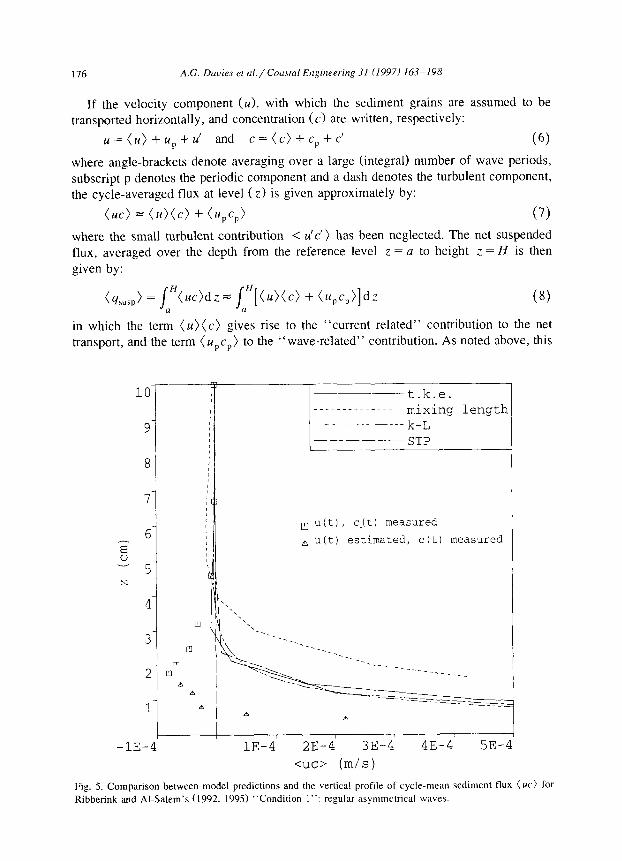
Beneath asymmetrical waves there is a net transport of sediment both in the near-bed, sheet flow, layer and in the outer suspension layer. As noted in Section 1, the magnitude and direction of the net transport is often strongly influenced by the so-called “wave-related” contribution and, in the absence of a significant current, is necessarily dominated by this effect. It should be added, however, that the detailed representation of any small residual currents (e.g., the near-bed current associated with the component U, in Eq. (5)) in model formulations can affect net transport calculations significantly, as shown recently by Davies and Li (1997).

176 A.G. Dauirs rt crl./Cocrstal Engineering 31 (1997) 163-198

If the velocity component (u), with which the sediment grains are assumed to be transported horizontally, and concentration (c) are written, respectively:

u=(u)+u,+u’ and c=(c) +cr+c’ (6)

where angle-brackets denote averagin, 0 over a large (integral) number of wave periods,

subscript p denotes the periodic component and a dash denotes the turbulent component, the cycle-averaged flux at level ( z) is given approximately by:

(UC) = (u)(c) + (upcp) (7)

where the small turbulent contribution < u’c’) has been neglected. The net suspended flux, averaged over the depth from the reference level z = a to height z = H is then

given by:

(qsusp) = /H(Uc)di= (“[(u>(c) + (n,c,)]dz u a

(8)

in which the term (U)(C) gives rise to the “current related” contribution to the net

transport, and the term (arcs> to the “ wave-related’ ’ contribution. As noted above, this

10

9

Y t.k.e.

---_----~~-____~~i~i~g length

_.__.._~.- k_L

_-_--- Srp

a

7 k

I q u(t), c_(t) measured 6 :

E _

A u(t) estimated, c(t) measured

I I , I -lE-4 lE-4 2E-4 3E-4 4E-4 5E-4

<UC> (m/s)

Fig. 5. Comparison between model predictions and the vertical profile of cycle-mean sediment flux (UC) for

Ribberink and Al-Salem’s (1992, 1995) “Condition I”: regular asymmetrical waves.

A.G. Davies et ul./Coasral Engineering 31 (1997) 163-198 177

latter term is likely to make the dominant contribution to the transport rate if (u) is very

small. In Fig. 5 the predicted vertical profiles of (UC) are compared with the data for the

Series C “Condition 1” experiment. Both the models and the data show “onshore” (positive) transport in the near-bed layer, and “offshore” (negative) transport in the outer suspension layer. [As indicated, the “measured” values of (UC) near the bed were based on measured values of c combined with estimated values of u, which could not

be measured reliably by the LDFM in the presence of the high sediment concentrations near the bed.] In fact, the net onshore transport was the dominant effect in the present

experiment, the offshore transport representing only about 5% of the total flux. Although there is qualitative agreement between the predicted profiles of (UC) and the data, the height of zero flux is overestimated by the various models by a factor of at least 4 times.

This is again indicative of the limitations of pure turbulence diffusion models in unsteady flows, and can probably be attributed to the neglect of convective effects at flow reversal in the model formulations. In the present case of “Condition l”, and also for the asymmetrical waves discussed below in Section 3.3, the net sediment transport was dominated by the flux in the near-bed layer. Any inaccuracy in the prediction of (UC) in the outer layer in these cases is therefore relatively unimportant in the

determination of ( qSuSP >.

3.3. Comparison with Ribberink and Al-Salem’s (1994) Series B experiments: regular

asymmetrical waves

The Series B experiments were carried out in the LOWT with a range of regular asymmetrical waves. Each experiment was again carried out in plane bed, sheet flow, conditions, and with the same sediment (D = 0.21 mm). The net transport rate was estimated from sediment traps and bed profiles. No time-dependent measurements were made in these earlier Series B experiments.

The total predicted and observed transport rates are plotted for the respective models in Fig. 6 for nine Series B experiments; for full details of the parameter settings, see Ribberink and Al-Salem (1994). Also included in Fig. 6 is the Series C “Condition 1” experiment discussed in Section 3.2, which is identified by a different plotting symbol. Perfect agreement between the model estimates and the experimental observations corresponds to the 45” line. It may be seen that each model predicts the sediment flux to within a factor of about 2 around this line, almost without exception. If an even more stringent test of model accuracy is applied, namely a factor of 13 around the perfect agreement line, the t.k.e, mixing length, k-L and STP models predict the net sediment flux within this band in lOO%, 60%, 70% and 90% of the 10 cases considered, respectively. As in the case of the “Condition 1” experiment, the net transport was dominated by the flux in the near-bed layer in each of the Series B cases. It should be recalled (see Section 2) that two of the four models (i.e. the STP and t.k.e. models) include a bedload transport estimate. In these cases the quantity plotted in Fig. 6 is:

(9) = (qsusp) +&I) (9)

where (qbed) corresponds to the net bedload transport in the height range 0 < z < a. In the case of the mixing length and k-L models, the quantity plotted is ( qSuS,). According

A.G. Dauics et ul./Coas~ul Engineering 31 (1997) 163-198

IO1 20 50 102 20

2" STP model

Units of <q>:

x10-’ m2 s-’

~9, computed

A.G. Daoies et al./ Coustul Engineering 31 (1997) 163-198 179

Table 2

Model input parameters for Series E experiments

Experiment (u) at z = 7.5 cm

Cm s- ‘1

El 0.150

E2 0.210

E3 0.285

E4 0.410

“1 (m s- ‘1

1.685 7.2

1.475 7.2

1.136 7.2

0.955 7.2

to the t.k.e. model results, the magnitude of (qsusP > is roughly twice that of ( qbed) in the present conditions.

Also included in Fig. 6 is a set of results obtained using an earlier version of the SIP model, in which the Engelund and Fredsoe (EF76 * > reference concentration formula has been used rather than ZF94 (see Fig. 6e). Since EF76 (or EF76 * > has been used in the

three other models (see Table 11, a comparison of the results in Fig. 6a-c and e, gives an indication of the differences which arise in (q) as a result of the differing representations of the turbulence diffusion process in the outer suspension layer in the respective models. This comparison is complicated, however, by the inclusion of graded sediment sizes in the earlier STP model. In fact, the predictions of the mixing length, t.k.e. and STP(EF76 * > models are rather similar, each model tending to overpredict (q)

somewhat. [The tendency of the k-L model to underpredict (q) in comparison with the other models is due to the fact that no estimate is included for ( qkd).] Evidently, the tendency of the STP model to overpredict (q) is largely removed if the reference concentration formula EF76 * (Fig. 6e) is replaced by ZF94 (Fig. 6d).

3.4. Comparisons with Katopodi et al.‘s (1994a,b) Series E experiments: combined

wave-current flow

The final experiments considered in this section were carried out more recently in the LOWT, following the addition of a recirculating-flow pumping system to the tunnel which allows a steady current to be added co-linearly to the waves (for details, see Katopodi et al., 1994a,b). In the Series E experiments, time-dependent measurements of u and c were made at various heights above the bed for four sinusoidal wave and current combinations (El to E4) under plane bed, sheet flow, conditions. These experimental conditions, which are defined in Table 2, were designed in such a way that, with increasing condition number (El + E4), the free-stream velocity amplitude of the wave (II,) decreased, while the cycle-averaged net current (u) increased. All four conditions may be considered to be wave-dominated cases. As indicated in the table, the matching level for (u) between the models and experiments was chosen as z = 7.5 cm. In experiments El-E4, the median grain size of the suspended sediment showed some

Fig. 6. Comparison between predicted ((9) or (qrusp). see Table 1) and observed net sediment transport rates for 9 of Ribberink and Al-Salem’s (1994) Series B experiments (0) and also for the Series C “Condition 1”

experiment (A). The fir11 45” line indicates perfect agreement. The dashed and dotted kws indicate factor * 1 f

and f 2 agreement bands, respectively.

180 A.G. Douies et crl./Coustal Engineering 31 (1997) 163-198

variation with height above the bed, from D = 0.21 mm near the bed to 0.18 mm for elevations z > 4 cm. In the STP model a settling velocity was calculated for each sediment size fraction in suspension (cf. Section 3.1). For the remaining model comparisons, the representative value of settling velocity ws = 0.025 m SK’ was used

(corresponding to D = 0.20 mm>, and the bottom roughness was taken as z,, = k,/30 = D/12 = 0.00175 cm.

Comparisons between the models and the measurements for the cycle-averaged

vertical profiles of horizontal velocity ( U) and sediment concentration ( c) are shown in Figs. 7 and 8, respectively. Each of the model predictions for (u) in Fig. 7 has been constrained to converge on the measured value at z = 7.5 cm and so, not surprisingly, the agreement with the data throughout the boundary layer is generally good. The only exceptions are El, and to a lesser extent E2, for which the velocity shear at the measurement levels is underpredicted.

No such constraint applies to the profiles of (c) in Fig. 8. Here the plotted data include both the concentration in the suspension layer (z 3 5 mm) measured with the OPCON, and the concentration in the sheet flow layer (z { 5 mm) measured with the CCM. It may be noted that a substantial jump in the values of (c) occurs at z = 5 mm, from the rather lower values measured with the OPCON to the much larger values measured with the CCM. This feature of the data has a very important influence on the results which follow. As in the earlier comparisons, level z = 0 corresponds to the undisturbed bed level prior to the start of the experiment. This choice for the origin of z_ is clearly important in defining the relationship between the model solutions and the data points, not only in Fig. 8 but also in the later figures.

Each of the models makes a reasonable estimate of (c) in the suspension layer, though there is a tendency for (c) to be overestimated, especially by the mixing length model. However, in the upper part of the sheet flow layer, where large concentration gradients arise, all of the models greatly underestimate (c). It should be noted that some inaccuracy may exist in the CCM data in this layer, for example as a result of possible errors of l-2 mm in the vertical positioning of the instrument. It may also be argued that inaccurate predictions of (c) in the sheet flow layer are to be expected, since all of the models represent the sediment as suspended load above a fixed reference level z = a = 20, with concentration governed solely by turbulence diffusion arguments. Detailed processes occurring in the sheet flow layer, including high concentration effects and vertical oscillations of the bed, are not represented in any of the models, though it may be noted that the reference concentration formulae used (see Table 1) necessarily incorporate features of the high-concentration layer, albeit indirectly.

Comparisons are made in Fig. 9 between the model predictions and time-series of concentration c( z_,t> measured at 8 levels above the bed in the case of experiment El (largest wave, smallest current). Velocity maxima in the free-stream correspond to t = T/4 and 3T/4. As expected from Fig. 8, the concentration in the upper sheet flow layers (z = 0.26, 0.56 and 0.65 cm; Fig. 9a> is underestimated by the models. However the phase variations in c are captured quite well at these heights, as is the small amount of asymmetry in c between successive wave half-cycles (i.e. larger concentrations in the second half-cycle when the wave motion was in the current direction). A significant deficiency in all of the model solutions is their inability to predict the large concentra-

A.G. Davies et d./Coastul Engineering 31 (1997) 163-198

P

(U=‘) 2

m N

-

1

mixing length

-..-..-..-..-..-

k_L

0 _-----_-----STP

10-l

10°

lo1

102

lo3

Concentration

(g/l)

10-l

loo

101

102

103

Concentration

(g/l)

0 -_______---_STP

10-l

10°

lOI

102

103

Concentration

(g/l)

10-l

loo

lOI

102

lo3

Concentration

(g/l)

-I

Fig.

8.

Com

pari

son

betw

een

mod

el

pred

ictio

ns

and

the

prof

ile

of c

ycle

-mea

n se

dim

ent

conc

entr

atio

n (c

) m

easu

red

by

Kat

opod

i et

al.

(199

4a,b

):

Seri

es

E,

co-l

inea

r

sinu

soid

al

wav

e an

d cu

rren

t fl

ow,

expe

rim

ents

(E

l -E

4)

as

indi

cate

d.

Time

(s)

600

2 500

\ m

; 400

.4

u a 300

2 G x 200

5

u

6 0

0 -

- -

..-...

m

easu

re’j

t.k.e.

z=O

.56

crq

,500

mixing len&h

ii

-..-..-..-..-..-

k_L

/ j

I :;

.

: : i‘i\.I ; I

. ..-

.....-

..... -.

.. m

eas”

red

t.k.e.

.._.__

mixing length

-._-..-.._..___

k_L

-___----___STP

1 2

3 Time

1 2

3

4

5

6

7

5

6

I

Time

(s)

Fig.

9.

C

ompa

riso

n be

twee

n th

e m

odel

pr

edic

tions

an

d tim

e-de

pend

ent

conc

entr

atio

ns

c(z,

t)

mea

sure

d ab

ove

the

orig

inal

be

d le

vel

(z

= 0)

by

K

atop

odi

et

al.

(199

4a,b

):

Seri

es

E,

expe

rim

ent

El,

co-l

inea

r si

nuso

idal

w

ave

and

curr

ent

flow

. T

he

com

pari

sons

fo

r th

e re

spec

tive

mod

els

are

mad

e:

(a)

at

thre

e re

pres

enta

tive

heig

hts

in t

he u

pper

sh

eet

flow

la

yer

(a

= 0.

26,

0.56

an

d 0.

65

cm);

an

d (b

) at

fiv

e he

ight

s in

the

su

spen

sion

la

yer

(z =

I .

45,

2.35

, 3.

65,

5.35

an

d 7.

1 cm

).

__...

......

......

. m

ixin

g le

ng

th

z=1.45 cm

_/ ‘-‘

-..

,: ‘..

,:

;.’

,.,’

r

1

2 3

4 5

6 I

Tim

e (s

)

7~

I-

1 2’

3r

4

5’

6 I’

Tim

e (s

)

45

_....

. -

- .._

... m

easu

red

J---

-z-

4 0

mix

ing

len

gth

z =2...,3

5 cm

,,..

'..,

,.I

.:' 'I.,,

.;'

“.

;:

'i.

2 35

-_.._

.._

.._..

-.._

k_

L

----

__--

----

S

T,F

’.-.’ . .

..,

1 r

1 2

3 4

5 6

7

Tim

e (s

)

1 2

3

4

5

6

I

Time

(s)

Fig

. 9

(con

tin

ued

).

A.G. Dauirs er ul./Cous~al Engineering 31 (1997) 163-198 185

_ _ __._. _ _.._ measured

2 12.5 .rl % 10.0 ,__.. .-...-- ._______ Y N__, ,/

(..’

6 -

7.5 ‘.._., ;.’

,:

s “.. .._..__

‘..___ ‘...._ ,..I ,. _,.___... . . . . . . . ..__.__.. .‘.. . .._..__ ,,.:’

8 5.0 ‘.. . . .._ ___ __.. .” .. ._.__ ~~‘..._..__. _,.:

1 2 3 4 5 6 7

Time (s)

Fig. 9 (continued).

(a) 2.5

2.0

1.5

E - 1.c N

0.5

0.c

suspension laye

pick-up la:

hta

2r

-0.2 -0.1 0.1 0.2 C

Sediment flux (m/s)

Fio IO. Comparison between (a) measured and (b) predicted, phase-averaged, vertical profiles of sediment

flti (UC) at eight instants during the wave cycle: Series E, experiment El.

186 A.G. Davies et ul./Crxxs~al Enginrering 31 (1997) 163-198

(b) 2.5

2.0

1.5

s - 1.0 N

0.5

l-0 i

!- -T/8 ----a T/ 4

b 3T/8

T/2 b 5Tl8

-.v- 3T/4

-mt-- lT/8,

El t.k.e.

-0.2 -0.1 0.1 0.2 0.3

2.5

2.0

1.5

% - 1.0 N

0.5

0.0

-0 _:

Sediment flux (m/s)

L E

-0.1 0.1 0.2 0.

Sediment flux (m/s)

Fig. 10 (continued).

A.G. Duuies er al./Coastal Engineering 31 (1997) 163-198

(b) 2.5

2.0 PST/t -3T/4

1.5

3 - 1.0 N

0.5

0.0

Sediment flux (m/s)

2.5

2.0

1.5

E - 1.0 N

0.5

0.0

STP El

-0.2 -0.1 0.1 0.2 0.3

Sediment flux (m/s)

Fig. 10 (continued).

187

188 A.G. Dauies ef al./ Cocrslal Engineering 31 (1997) 163-198

r ; : I

cc P u3 tr -3 m N

(“3) =

8’c c

-4E

-4’

4E-4'

8E-4

12E-k

16E-4

20E-4' 24E-.

Sediment

flux

(m/s)

81

7 6

-z5

u4

N

I

3 2 1 L E

3

‘._ ‘\

‘...

‘....

~

OE-4

4E-4

BE-4

12E-4

16E-4

20E-4

243-4

Sediment

flux

(m/s)

8

7

6

T5

v4

N

3

2

1

8

7

6

T5

v4

N

3

2

1

I r-

q

Measured

._........__.__._....~-._~.~~.~..

mixing

length

_._-.._..-..-.--

l&_L

-----_____-_STP

E2

I

OE-4

4E-4

BE-~

12E-4

16~-4' 20E-4

243-4'

Sediment

flux

(m/s)

‘4

OE-

4E-4

BE-~

12E-4

16E-4

20E-4

24E-1

Sediment

flux

(m/s)

Fig.

12

. C

ompa

riso

n be

twee

n pr

edic

ted

([in

es)

and

mea

sure

d (s

ynzh

ok),

cy

cle-

aver

aged

, ve

rtic

al

prof

iles

of

tota

l fl

ux

(UC

) in

th

e su

spen

sion

la

yer:

Se

ries

E

,

expe

rim

ents

E

l-E

4.

The

res

pect

ive

figu

res

show

th

e pr

edic

ted

prof

iles

of

(UC

) fo

r th

e fo

ur

mod

els

for

expe

rim

ents

E

l-E

4.

190 A.G. Dauirs er d./Coa.stul Enginerring 31 (1997) 163-198

tion peak at each flow reversal (t = 0 and T/2). The origin of this peak may be seen very clearly in the upper sheet flow layer. It then propagates up as a “convection” peak (cf. Section 3.1) into the suspension layer, where it “widens” (Z = 1.45 cm), and then coalesces with the basic “diffusion” peak at the higher measurement levels (Fig. 9b). As in the earlier case of “Condition 3”, the models capture the diffusion peak reasonably well in the lower part of the suspension layer (2 = 1.45 cm). Here, in

general, the models are in quite good agreement with concentration measured by the OPCON. But, as noted above, they fail to predict the convection peak at flow reversal, resulting in rather poor agreement between the models and the measurements in the upper part of the suspension layer (z > 2.35 cm).

Since the present models do not represent processes occurring in the upper sheet flow layer, it is to be expected that their detailed predictions of the suspended sediment flux will differ from the measurements. This is seen in Fig. 10 in which a comparison is

made for experiment El between predicted and measured, phase-averaged, vertical profiles of sediment flux (UC) at eight instants during the wave cycle. The measured profiles (Fig. 1Oa) show transport occurring not only in the suspension and sheet flow layers, but also in the “pick-up layer” (i.e. z < 1 mm). The measurements also display pronounced asymmetry, particularly in the sheet flow layer, with large positive fluxes corresponding to the half-cycle (T/2 < t < T) in which the (positive) wave motion is superimposed on the (positive) current. As far as the predictions (Fig. lob) are concerned, each model is constrained by the assumption of no-slip at the zO-level, where the flux must be zero. Above this some asymmetry does occur in the uc-profiles for the reasons given above, and the peak values of UC in 0 < z < 1 cm are of the same magnitude as the peak values measured in the sheet flow layer. But the predicted values of UC in the upper sheet flow layer are too small according to the data. This is not surprising in view of the large values of c measured at these heights (Figs. 8 and 9a).

The cycle-averaged vertical profiles of suspended sediment flux are shown in Figs. 11 and 12. In Fig. 11 profiles of total sediment flux (UC) are shown for the respective models for experiment El, together with profiles for the “current-related” (( u)( c>> and “wave-related” ((u,c,>> contributions. In Fig. 12 the predicted profiles of (UC) are compared with the data for experiments El to E4, respectively. As in the case of the asymmetrical waves discussed earlier (“Condition I”, Section 3.2), the measured profiles for El and E2 display a reversal in the direction of net transport in the suspension layer. In the lower suspension layer the flux is in the current direction while, at heights above about 3 cm, the transport is in the opposite direction due to the dominance of the wave-related contribution. This effect becomes less pronounced in E3 and E4 in which the wave velocity amplitudes, and hence wave-related transport, are less important. In a qualitative sense, the models capture the main features of the net transport profiles, as was found earlier for the asymmetrical waves (see Fig. 5). But, once again, the height of the change in direction of (UC) is overestimated (at least for El and E2) by a factor of 2 or more. More generally, the models tend to overpredict (UC), which is not surprising in view of their tendency to overpredict (c) in the suspension layer (see Fig. 8).

In view of the many limitations of the model predictions highlighted above, it might be expected that poor agreement would be found between the predicted total (i.e.

A.G. Dauics et ul./Cou.stul Engineering 31 (1997) 163-198 191

t.k.e. 200

<CP computed

Units of <q>: x10m6 m* s-’

Fig. 13. Comparison between predicted (( q) or ( qs >, as indicated) and observed net sediment transport rates

for Katopodi et al.‘s (1994a, b) Series E experiments. The Jill 45” line indicates perfect agreement. The

&shed and dotred lines indicate factor f 1; and k 2 agreement bands, respectively.

temporally and vertically integrated) sediment transport rate and the values measured in the four Series E experiments. In fact, this turns out not to be the case, as shown in Fig. 13 and Table 3. (Here the “measured” values of (q) are slightly corrected estimates of transport, corresponding to conditions along the centre-line of the LOWT. The correc-

tion has been made to account for side-wall effects in the tunnel in the presence of a current, and allows a better basis for comparison between the observations and the models.) The model predictions of total transport in Table 3 all lie within a factor of 2 of the measured values. In fact, the results for the STP model all lie within 4% of the measured values, the corresponding figures for the k-L, t.k.e. and mixing length models being 20%, 28% and 86%, respectively. The tendency for (q) to be overpredicted by the mixing length model may again be attributed to its overprediction of (c) (see Fig.

192 A.G. Douirs et aI./ Coustul Engineering 31 (1997) 163-198

Table 3 Measured and predicted net sediment fluxes (q) (X 10m6 m’ s- ‘) for the Series E experiments

Experiment Measured flux, Models

(q) mixing length STP tke. k-L

(q) (%“*J ((I) (%“S[,) (q)

( %usp )c ( > (surp) ((1) (Ysusp)

‘lsurp c (%“SP)C (q > ( qsusp )w ( Ysusp )w (%usp)w

susp c (Ysusp)w

El 107.2 163.6 163.6 104.2 98.3 I 11.7 78.4

102.4 38.3 38.4

61.2 60.0 40.0

E2 111.8 170.4 170.4 II I.5 103.1 112.6 78.8

97.4 37.7 32.6

73.0 65.4 46.2

E3 80.8 144.7 144.7 17.5 66.3 103.7 71.4

68.5 22.4 26.0

76.2 43.9 45.4

E4 84.4 157.2 157.2 83.7 66.9 106.6 72.6

74.8 27.7 30.3

82.4 39.2 42.3

109.2 109.2

36.8

72.3

III.8 III.8

37.5

16. I

73.8 73.8

22.1

51.7

67.5 67.5

22.4

45.0

The suspended load contribution to each predicted value of (q>, and its breakdown into current- and

wave-related components, is also tabulated.

8). As noted earlier, the STP and t.k.e. models include both suspended load and bedload transport components. For the STP model, the suspended load contributes 80-94% of the total transport in experiments El -E4; for the t.k.e. model the corresponding figures are 68-70%. (For the remaining models, the values of (q) and ( qsusp) in Table 3 are identical, since a bedload component is not included.)

4. Discussion

The predictions of the four turbulence diffusion models for the net sediment transport rates ((q)) measured beneath asymmetrical waves (Section 3.3) and combined waves and currents (Section 3.4) would be considered extremely good in coastal engineering practice. It should be noted, however, that all of the situations considered earlier involved the one common sand size D = 0.21 mm (fine sand), for which (q) was dominated by near-bed transport in the sheet flow and lower suspension layers, with only a relatively small contribution being made by the outer suspension layer. In other words, the accuracy of the estimates of concentration in the outer layer was of relatively little practical importance. For finer sediment sizes in suspension, the situation may be expected to be rather different. This has been demonstrated by Ribberink and Chen (1993) who carried out experiments in the LOWT with large asymmetrical waves above

. a plane sand bed of gram stze D,, = 0.13 mm. The importance of transport in the outer suspension layer has also been demonstrated in wave and current conditions, similar to

A.G. Douies et al./ Coastul Engineering 31 (1997) 163-198 193

those discussed earlier, by Murray et al. (1991) using the grain size D = 0.12 mm. In this series of combined flow experiments above plane beds, the net flux (q) was shown to be influenced strongly by a negative wave-related contribution to the suspended sand transport in the approximate height range 1- 10 cm.

The success of the four turbulence diffusion models in predicting (q) with consider-

able accuracy may be contrasted with the failure of any of the models to represent the details of the time- and height-varying sediment concentration satisfactorily. In particu- lar, none of the present models represents the peaks in suspended sediment concentration which were measured at flow reversal. This apparent inconsistency is explained by the fact that (q) was dominated by near-bed processes and that, at the times in the wave cycle when the concentration peaks occurred, the flow velocities were small. It may be noted that, in the laboratory experiments of Murray et al. (1991) and Ribberink and Chen (1993) convective effects at flow reversal were far more pronounced than any seen in the concentration data discussed in Section 3. Moreover, they were found to have an important effect on the net sediment transport, by influencing the concentration for a significant period during the half-cycle after their initial appearance. In the combined flows studied, the effect of the large convective peak observed at flow reversal following the wave + current half-cycle was to enhance the wave-related component of transport in the negative direction (i.e. in the direction opposing the current). In a similar way, the large convective peak occurring after the passage of the crest of an asymmetrical wave will tend to enhance suspended concentrations at the time in the wave cycle when transport is in the offshore direction, and so enhance the offshore wave-related transport.

At the present time, there are no well-established modelling methods to account for convective effects of the type described above. The simulation of Ribberink and Al-Salem’s asymmetrical wave “Condition 1” carried out by Black (1994) produced very good agreement with the measured concentrations by use of a strongly, and discontinuously, time-varying eddy viscosity. Unfortunately, no general rules applicable in other situations may be inferred from Black’s study. However, the need for modelling approaches to account for convective effects arising from oscillatory boundary layer instabilities in the adverse pressure gradient conditions leading up to flow reversal seems unquestionable. As noted earlier, each of the present models assumes that the boundary layer remains thin and well behaved throughout the wave cycle, whereas the sediment concentration data suggest a breakdown of the oscillatory boundary layer structure at around the time of flow reversal. In the absence of any measurements of the near-bed velocity field to accompany the detailed concentration time-series in Figs. 1 and 9, the explanation for the convective peaks remains rather unclear.

Since all of the experiments considered in this study were carried out above plane beds and at high wave Reynolds numbers (Re = lJF/ov 3 3 X IO’, where u = kinematic viscosity), conventional turbulence modelling schemes might be expected to act as a good starting point to describe the oscillatory boundary layer phenomena observed (except possibly around times of flow reversal). This statement would certainly be true if the present wave conditions were imposed above a flat, “not too rough”, immobile bed, since momentum transfer would be dominated by random turbulent processes in these circumstances. Only above “very rough” immobile beds, and at rather lower values of

194 A.G. Daures et ol./Coustul Engineering 31 (1997) 163-198

Re, is momentum transfer known to be dominated by well-organised, periodic, convec- tive events associated with eddy shedding from individual roughness elements at flow reversal (e.g., Sleath, 1987). Yet, at high Re values above a mobile oscillating sheet flow layer, some analogous form of well-organised momentum transfer, leading to convective sediment entrainment, has now been observed in several different experi- ments. It is possible that the techniques which have been proposed for modelling oscillatory flow above very rough immobile beds (Sleath, 1991; Nielsen, 1992; Davies and Villaret, 1997) may prove to be applicable also in these mobile bed situations.

The present turbulence diffusion modelling schemes have two further limitations which should be mentioned briefly. First, the use of a time-varying sediment reference

concentration presents great uncertainties, even above flat beds. All of the present models utilize, in a quasi-steady manner, a reference concentration formula derived for

steady flow conditions. As noted in Section 2, this is questionable conceptually, and some advantages may be gained by using the alternative “pick-up function” form of unsteady bottom boundary condition for the suspended sediment. In addition, the particular assumptions under which steady flow reference concentrations are derived (e.g., logarithmic mean velocity profile, no damping of turbulence by sediment) make it difficult to incorporate in models, in a consistent way, potentially important processes such as turbulence damping and hindered settling. It should be noted, however, that these two effects are accounted for, albeit indirectly, in the reference concentration formula ZF94 used in the STP model. (This formula has been designed for practical use, based on conventional logarithmic velocity and Vanoni-type concentration profiles, even in situations in which stratification effects are important.)

Second, the four models discussed in this paper are primarily models of sediment in suspension, and they do not include physical processes which occur in the high-con- centration, sheet flow, layer. Although the STP and t.k.e. models do represent bedload transport, this is achieved only by the quasi-steady use of a bedload transport rate formula, derived for steady flow conditions. The consistency of this approach in terms of the choice of a matching level between the bedload and suspended load layers is highly questionable. However, the use of more consistent two-phase modelling ap- proaches to provide a continuous description of processes from the immobile bed, though the sheet flow layer, and into the suspension layer, is not yet well established. The future use of two-phase flow models should, in principle, overcome present uncertainties such as the definition of the origin of height (z> in comparisons between model results and data.

5. Conclusions

The predictions of four sediment transport models have been compared with labora- tory data obtained above plane beds in an oscillating water tunnel. The measurements were made beneath regular symmetrical and asymmetrical waves, and also in wave- dominated combined wave and current flows. The hydrodynamical conditions both in the experiments and in the model simulations were horizontally uniform. In terms of their predictions for the net (i.e. temporally and vertically averaged) sediment transport rate, each of the models agrees with the measured values to within a factor of 2 in

A.G. Davies et ul./Coa.stal Engineering 31 (19971 163-198 195

almost every case. If the models are assessed according to a more stringent criterion involving a factor of 1; around the measured value, their relative performance may be judged from Figs. 6 and 13.

By the standards existing in coastal engineering practice, the accuracy achieved by the models in terms of the net sediment transport rate is very good indeed. However, this may be due in large part to the sand size (D = 0.2 mm) considered throughout this study, for which transport was dominated by processes in the sheet flow and lower suspension layers, enabling the models to make accurate predictions of the net transport. It is likely that significantly less good agreement would have been achieved had the experiments been carried out with finer sediment in the same wave and current conditions, since transport in the outer suspension layer would then have been of greater

relative importance. The underlying weaknesses of the models used here, and of all other models based on

conventional turbulence diffusion arguments, have been revealed by the comparisons made with detailed time-dependent measurements of sediment concentration. First, each of the models is aimed primarily at the prediction of the sediment distribution in the low concentration suspension layer; none of the models represents conditions in the high concentration upper sheet flow layer. Second, even in the high wave Reynolds number, sheet flow, conditions studied here, convective mechanisms have been shown to play an important role in entraining sediment into suspension. None of the models is able to represent the phenomenon of convective entrainment at flow reversal, which arises from instability in the oscillatory sheet flow layer and affects the time-varying sediment concentration in both the sheet flow and suspension layers. The potential importance of this effect in relation to the “wave-related” net sediment transport is now well established, and has been demonstrated here, albeit indirectly, through the shortcomings of the model predictions in comparison with detailed measurements of time-dependent sediment concentrations and fluxes during the wave cycle (Figs. 1, 9 and 10).

The initial aim of this intercomparison was to assess the relative strengths and weaknesses of four models based on more or less sophisticated modelling schemes for the turbulence. In fact, some of the differences between the model predictions have been found to be rather small compared with the differences between the models and the observations. Moreover, the scatter and uncertainty in the data have, in some instances, been comparable with the variation in the model predictions. Although the physical processes represented by the individual models are rather different (e.g., one model includes graded sediment effects, two models include turbulence damping by suspended sediment, and so on - see Table 11, it is not possible on the basis of the results discussed here to argue strongly for the use of one model in preference to another. Certainly, on the present evidence, no clear-cut case can be made for the advantages of sophisticated turbulence closure schemes, since the simpler models perform just as well. However, it is possible that the more sophisticated schemes would be the more accurate ones in conditions dominated by suspended sediment transport, particularly if the mechanism of convective entrainment at flow reversal was included in the model formulation.

In order to advance our knowledge of sediment transport above plane beds, and hence improve the accuracy of predictive modelling schemes, new experimental research is

196 A.G. Dauks et d./Cou.stal Engineering 31 (1997) 163-198

required to determine, in the first place, the velocity field within the oscillatory sheet flow layer, to accompany our existing knowledge of the concentration field. [Such oscillatory flow measurements have been made by Dick and Sleath (1991) using light-weight particles, but no comparable measurements have yet been made for cases involving sand grains.] It should be possible to use such data to define improved bottom boundary conditions for the suspension layer (e.g., improved pick-up functions), as well as to obtain soundly based formulations for the (time-varying) hydraulic roughness of

the bed. In addition, by use of measurements of the vertical velocity field at times of flow reversal, it should be possible to develop convection-diffusion arguments which

properly represent sediment entrainment throughout the wave cycle. Ultimately, by the use of sophisticated two-phase flow models, it should be possible to obtain a continuous description of grain-grain and fluid-grain interactions from the stationary bed, into the collision (i.e. sheet flow) layer, and then upwards into the suspension layer.

Acknowledgements

This study was carried out as part of the MAST2 G8-M Coastal Morphodynamics project, supported financially by the Commission of the European Communities, Direc- torate General for Science, Research and Development under contract number MAS2- CT92-0027. Much of the work was also co-sponsored by national funding agencies, including: - UK Ministry of Agriculture, Fisheries and Food (Contract CSA2288) - Dutch Ministry of Transport and Public Works (Coastal Genesis) - French Programme Nationale d’oce’anographie C6tiere (PNOC) - Danish Technical Research Council (STVF)

The authors are greatly indebted to the following people for their help during the preparation of this paper: at UCNW, Zihong Li and Andy Peet; at Delft Hydraulics, Marjolein Janssen; and, at L.E.G.I., Tran Thu Tam. The authors would also like to thank their colleagues in the MAST2 project, especially those in “Working Group D: Wave-Current-Sediment Interaction”, for their contributions and discussions. Particu- lar thanks are extended to Jorgen Fredsoe, Richard Soulsby, Mutlu Sumer, Jan van de Graaf and Leo van Rijn, for their helpful comments.

References

Bailard, J.A., 1981. An energetics total load sediment transport model for a plane sloping beach. J. Geophys. Res., 86(Cl I): 109X-10954.

Bakker, W.T., 1974. Sand concentration in an oscillatory flow. Proc. 14th Int. Conf. on Coastal Engineering, Copenhagen, Am. Sot. Civ. Eng., New York, NY, pp. I l29- I 148.

Black, K., 1994. Suspended sediment load during an asymmetric wave cycle over a plane bed. Coast. Eng., 23:

95-114.

Brors, B. and Eidsvik, K.J., 1994. Oscillatory boundary layer flows modelled with dynamic Reynolds stress turbulence closure. Cont. Shelf Res., 14: I455 1475.

Davies, A.G., 1995. Effects of unsteadiness on the suspended sediment flux in colinear wave-current flow.

Cont. Shelf Res., 15(8): 949-979.

A.G. Davies et crl./Coustul Engineering 31 (1997) 163-198 197

Davies, A.G. and Li, Z., 1997. Modelling sediment transport beneath regular symmetrical and asymmetrical

waves above a plane bed. Cont. Shelf Res., 17(5): 555-582.

Davies, A.G. and Villaret, C., 1997. Oscillatory flow over rippled beds: Boundary layer structure and

wave-induced Eulerian drift. In: J.N. Hunt (Editor), Gravity Waves in Water of Finite Depth, Ch. 6.

Advances in Fluid Mechanics, Computational Mechanics Publications, pp. 215-254.

Davies, A.G., Eidsvik, K.J., Ribberink, J.S., Temperville, A. and Zyserman, J.A., 1994. Intercomparison of

models of wave-current-sediment interaction. MAST2 G8-M Coast. Morphodyn. Proj., Gregynog Overall

Workshop, Sept. 1994, Abstr. 3.14, 4 pp., published by Delft Hydraulics, Delft.

Dick, J.E. and Sleath, J.F.A., 1991. Velocities and concentrations in oscillatory flow over beds of sediment. J.

Fluid Mech., 233: 16.5-196.

Engelund, F. and Fred%%, J., 1976. A sediment transport model for straight alluvial channels. Nord. Hydrol.,

7: 293-306.

Fredsoe, J., 1984. Turbulent boundary layers in wave-current motion. Proc. Am. Sot. Civ. Eng., J. Hydraul.

Eng., 110: 1103-l 120.

Fredsoe, J., 1993. Modelling of non-cohesive sediment transport processes in the marine environment. Coast.

Eng., 21: 71-103.

Fredsoe, J., Andersen, O.H. and Silberg, S., 1985. Distribution of suspended sediment in large waves. Proc.

Sot. Am. Sot. Civ. Eng., J. Waterway, Port, Coast. Ocean Eng., 11 l(6): 1041-1059.

Glenn, SM. and Grant, W.D., 1987. A suspended sediment stratification correction for combined wave and

current flows. J. Geophys. Res., 92(C8): 8244-8264.

Hagatun, K. and Eidsvik, K.J., 1986. Oscillating turbulent boundary layer with suspended sediments. J.

Geophys. Res., 91(Cll): 13045-13055.

Huynh Thanh, S., Tran Thu, T. and Temperville, A., 1994. A numerical model for suspended sediment in

combined currents and waves. In: M. Belorgey, R.D. Rajaona and J.F.A. Sleath (Editors), Sediment

Transport Mechanisms in Coastal Environments and Rivers. EUROMECH 310, Le Havre, Sept. 1993,

World Scientific, Singapore, pp. 122- 130. Katopodi, I., Ribberink, J.S., Ruol, P., Koelewijn, R., Lodahl, C., Longo, S., Crosato, A. and Wallace, H.,

1994a. Intra-wave sediment transport in an oscillatory flow superimposed on a mean current. Delft

Hydraulics, Delft, Rep. H-1684, Part III.

Katopodi, I., Ribberink, J.S., Ruol, P. and Lodahl, C., 1994b. Sediment transport measurements in combined

wave current flows. Proc. of Coastal Dynamics ‘94, Barcelona, Am. Sot. Civ. Eng., New York, NY, pp.

837-851. Li, Z. and Davies, A.G., 1996. Towards predicting sediment transport in combined wave-current flow. Proc.

Am. Sot. Civ. Eng., J. Waterway, Port, Coast. Ocean Eng., 122(4): 157-164. Madsen, O.S., 1991. Mechanics of cohesionless sediment transport in coastal waters. Proc. of Coastal

Sediments ‘91, Am. Sot. Civ. Eng., New York, NY, pp. 15-27.

Meyer-Peter, E. and Muller, R., 1948. Formulas for bed-load transport. In: Report of 2nd Meeting of the International Association of Hydraulic and Structural Research, Stockholm, pp. 39-64.

Murray, P.B., Davies, A.G. and Soulsby, R.L., 1991. Sediment pick-up in wave and current flows. In: R.L.

Soulsby and R. Bettess (Editors), Proceedings of EIJROMECH 262 Colloquium on Sand Transport in

Rivers, Estuaries and the Sea, Wallingford, June 1990, Vol. 1. A.A. Balkema, Rotterdam, pp. 37-43. Nielsen, P., 1991. Combined convection and diffusion: a new framework for suspended sediment modelling.

Proc. of Coastal Sediments ‘91, Seattle, WA, Vol. 1. Am. Sot. Civ. Eng., New York, NY, pp. 418-431.

Nielsen, P., 1992. Coastal Bottom Boundary Layers and Sediment Transport. World Scientific, Singapore, 324

PP. Ribber-ink, J.S. and Al-Salem, A.A., 1992. Time-dependent sediment transport phenomena in oscillatory

boundary layer flow under sheet-flow conditions. Delft Hydraulics, Delft, Data Rep. H 840.20, Part VI, Dec. 1992, 130 pp.

Ribberink, J.S. and Al-Salem, A.A., 1994. Sediment transport in oscillatory boundary layers in cases of rippled beds and sheet flow. J. Geophys. Res., 99(C6): 12707- 12727.

Ribberink, J.S. and Al-Salem, A.A., 1995. Sheet flow and suspension of sand in oscillatory boundary layers.

Coast. Eng., 25: 205-225. Ribberink, J.S. and Chen, Z., 1993. Sediment transport of fine sand under asymmetric oscillatory flow. Delft

Hydraulics, Delft, Data Rep. H 840.20, Part VII, Jan. 1993.

198 A.G. Dauirs et ul./ Cocr.stcrl Engineering 31 (1997) 163-198

Rubey, W.W., 1933. Settling velocities of gravel, sand and silt. Am. J. Sci., 25: 325-338.

Sleath, J.F.A., 1987. Turbulent oscillatory flow over rough beds. J. Fluid Mech., 182: 369-409.

Sleath, J.F.A., 1991. Velocities and shear stresses in wave-current flows. J. Geophys. Res., 96(C8):

15237- 15244. Soulsby, R.L., 1991. Aspects of sediment transport by combined waves and currents. Hydraul. Res.,

Wallingford, Hydraul. Res. Publ. Pap. No. 54, 14 pp.

Soulsby, R.L., Hamm, L., Klopman, G., Myrhau,, 0 D., Simons, R.R. and Thomas, G.P., 1993. Wave-current

interaction within and outside the bottom boundary layer. Coast. Eng., 21: 41-69.

van Rijn, L.C., 1991. Sediment transport in combined currents and waves. In: R.L. Soulsby and R. Bettess

(Editors), Proceedings of EUROMECH 262 Colloquium on Sand Transport in Rivers, Estuaries and the

Sea, Wallingford, June 1990, Vol. I. A.A. Balkema, Rotterdam, pp. 3-15.

van Rijn, L.C., Nieuwjaar, M.W.C., van der Kaay, T., Nap, E. and van Kampen, A., 1993. Transport of fine

sands by currents and waves. Proc. Am. Sot. Civ. Eng., J. Waterway, Port, Coast. Ocean Eng., 119(2):

123-143.

Villaret, C. and Perrier, G., 1992. Transport of fine sand by combined waves and current: an experimental

study. Electr. Fr., Rep. No. HE-42/92.68, 81 pp.

Vincent, C.E. and Green, M.O., 1990. Field measurements of the suspended sand concentration profiles and

fluxes and of the resuspension coefficient y0 over a rippled bed. J. Geophys. Res., 95(C7): 11591-I 1601.

Zyserman, J.A. and Fredsoe, J., 1994. Data analysis of bed concentration of suspended sediment. Proc. Am. Sot. Civ. Eng., J. Hydraul. Eng., 120(9): 1021-1042.

Zyserman, J.A. and Fredsoe, J., 1996. Validation of a deterministic sediment transport model for sheet-flow

conditions. Inst. Hydrodyn. Hydraul. Eng. (ISVA), Tech. Univ. of Denmark, Lyngby, Progr. Rep. 76, July

1966, pp. 3-9.