comparison study of flow in a compound channel

ITB J. Eng. Sci. Vol. 39 B, No. 2, 2007, 67-97 67

Received August 13th, 2007, Revised March 13th, 2008, Accepted for publication March, 25th, 2008.

Comparison Study of Flow in a Compound Channel: Experimental and Numerical Method Using Large Eddy

Simulation SDS-2DH Model

Eka Oktariyanto Nugroho1 & Syunsuke Ikeda2

1 Water Resources Engineering, Study Program of Civil Engineering, 0Faculty of Civil and Environmental Engineering, Bandung Institute of Technology

2 Professor, Department of Civil and Environmental Engineering, 1Tokyo Institute of Technology, Japan

Abstract. Flow modeling in a compound channel is a complex matter. Indeed, due to the smaller velocities in the floodplains than in the main channel, shear layers develop at the interfaces between two stage channels, and a momentum transfer corresponding to this shear layer affects the channel conveyance. Since a compound channel is characterized by a deep main channel flanked by relatively shallow flood plains, the interaction between the faster fluid velocities in the main channel and the slower moving flow on the floodplains causes shear stresses at their interface which significantly distort flow and boundary shear stress patterns. The distortion implies that flow field in rivers is highly non homogeneous turbulent, which lateral transport of fluid momentum and suspended sediment are influenced by the characteristics of flow in rivers. The nature of mechanism of lateral transport needs to be understood for the design of river engineering schemes that rely upon realistic flow. Furthermore, the flows in river are also almost turbulent. This means that the fluid motion is highly random, unsteady, and three-dimensional. Due to these complexities, the flow cannot be properly predicted by using approximate analytical solutions to the governing equations of motion. With the complexity of the problems, the solution of turbulent is simplified with mathematics equation. The momentum transfer due to turbulent exchanges is then studied experimentally and numerically. Experimental data is obtained by using Electro Magnetic Velocimetry and Wave Height Gauge. The Large Eddy Simulation Sub Depth Scale (LES SDS)-2 Dimensional Horizontal (2DH) Model is used to solve the turbulent problem. Successive Over Relaxation (SOR) method is employed to solve the numerical computation based ob finite difference discretization. The model has been applied to the compound channel with smooth roughness. Some organized large eddies were found in the boundary between main channel and flood channel. At this boundary the transverse velocity profile exhibits a steep gradient, which induces significant mass and momentum exchange, acts as a source of vorticity, and generates high Reynolds stresses.

68 Eka Oktariyanto Nugroho & Syunsuke Ikeda

The Large Eddy Simulation SDS-2DH model enables to predict quite successfully the wavelength of some observed vortices. The estimated vortex wavelengths agree again with the measurements and the theoretical predictions. The present model is proven to be a useful tool for engineering applications, as it can simulate the dynamic development of large eddies.

Keywords: compound channel; LES model; SOR; SDS-2DH; turbulent; two dimensions flow.

1 2Introduction The flow in channel or a conduit having a free surface is called free surface flow or open channel flow. Flow in rivers, streams, irrigation or power canals, flumes, chutes, aqueducts, spillways and drainage ditches are typical examples of free surface flow. For many problems encountered by hydraulic engineers, the analysis of free surface flow is required, e.g., heat and mass transport, dispersion and dilution of pollutants, flood forecasting, erosion and siltation of rivers and man-made canals.

A compound channel is a naturally occurring feature of any river or stream. Many rivers consist of a channel with adjacent floodplains. The bottom of the floodplain is generally higher and rougher than the bottom of the main channel, so that during flood the river consists of a relatively deep channel and shallow floodplains, a so-called compound channel. The word compound refers to the channel's ability to handle two stages of flow: normal flow and flood flow. Some of the main hydraulic features of compound channel flow are shown in Figure 1 for a symmetric two-stage channel with a trapezoidal cross-section.

Since a compound channel is characterized by a deep main channel flanked by relatively shallow flood plains, the interaction between the faster fluid velocities in the main channel and the slower moving flow on the floodplains causes shear stresses at their interface which significantly distort flow and boundary shear stress patterns. The distortion implies that flow field in rivers is highly non homogeneous turbulent, which lateral transport of fluid momentum and suspended sediment are influenced by the characteristics of flow in rivers. The nature of mechanism of lateral transport needs to be understood for the design of river engineering schemes that rely upon realistic flow or sediment routing models. This mechanism of real flow at river can be seen in Figure 2.

Furthermore, flows in river are mainly categorized as shallow water flows in which the horizontal scale of flow geometry is much larger than the vertical scale. Also the flows in river are almost turbulent. This means that the fluid motion is highly random, unsteady, and three-dimensional. Due to these

Comparison Study of Flow in a Compound Channel 69

complexities, the flow cannot be properly predicted by using approximate analytical solutions to the governing equations of motion. With the complexity of the problems, the solution of turbulent is simplified with mathematics equation.

Turbulent fluctuations are then approximated by a suitable averaging of the governing equations. These averaged equations describe the complete effect of turbulence on the average motion. This representation is usually referred to as turbulence modeling.

Figure 1 Hydraulic parameters associated with floodplain flow in a compound channel (Shiono, K. & Knight, D.W., [1]).

Direction of flow

Figure 2 Vortices at the interface between the main channel and floodplain flow, Medicine Hat, Alberta (Tuitoek, D.K., [2]).


2 3Methodology

2.1 6Experimental Set Up In order to support the experimental part of this work, the tilting laboratory flume is used. This flume is 40 cm wide, and its overall length equals 1400 cm. The longitudinal slope of the bed is 0.001. The major hydraulic variables are summarized in Table 1. Sketch and picture of the laboratory flume cross section are shown in Figure 3 and Figure 4.

Tabel 1 Major hydraulic variables of experiments.

Channel length (L) Channel width (B) Main channel width (Bm) Flood channel width (Bf) Main channel depth (Hm) Flood channel depth (Hf) Longitudinal Bed Slope (I)

1400 cm 40 cm 24 cm 16 cm 6.2 cm 1.2 cm 1.0 x 10-3

24 cm

Bm

16 cm

Bf

Flow direction

Figure 3 Laboratory flume cross section.

The performed measurements include: (1) water level and (2) velocity. The water levels were measured using an automatic wave height gauge (WHG) mounted on the measurement trolley. The electromagnetic velocimetry (EMV) is used for measuring velocity in the edge boundary of flood channel and main channel.

The frequency for obtaining the data is put to 100 Hz with 30 second time recording. Velocity measurements are conducted in transverse direction of the channel for 2 cm interval while height measurement is done for one point near the boundary of main and flood channel. The location of both measurements can be seen in Figure 4.


x (m)

y (m)

0 2 4 6 8 10 12 14

flood channel (Bf)

main channel (Bm)

location of measurement

6.4

water tank circulationflow direction

water tank circulation

A

A

16

40

A

A

16 cm

24 cm

Bf

Bm

position of WHG

1 cm

EMV, 2 cm interval

16 cm24 cm

Hf = 1.2 cm

WHG

Hm = 6.2 cm

BfBm

1 cm

1 cm

EMV

1 cm

2 cm interval

Figure 4 Channel sketch, plan view, cross section (A-A) and location of measurement.

2.2 7Numerical Method (LES SDS – 2DH)

2.2.1 1 2Large Eddy Simulation (LES) Method LES is a compromise between DNS and RANS. The main idea behind LES is to filter out the fine or high frequency scales of motion and leave the large scales to be solved directly, while the effects of the small eddies on the large eddies are modeled (by using model such as Smagorinsky model, buoyancy-modified Smagorinsky model, structure function model, etc). This approach is motivated by one of the most important features of turbulent flows, irregularity. Indeed, homogenous, isotropic turbulence (when sufficiently far away from the walls) is believed to have a random nature. The fact that it is random suggests that it has a universal character and the effects of the smaller scales should be capable of being represented by a model and thus predictable. On the other hand, the larger eddies in a turbulent flow are widely believed to be deterministic, hence predictable once the effects of the smaller eddies on them is known.


Furthermore, these larger eddies are often the most important flow structures and carry the most energy.

The LES method consist the following steps:

1. decompose flow variables into large and small scale parts, with the large scale part purportedly defined by a filtering process;

2. filter the governing equations, and substitute the decomposition from part 1 into the nonlinear terms to construct the unclosed terms to be modeled;

3. model these unresolved stresses; 4. solve for the large-scale contribution (while essentially ignoring the small-

scale part).

2.2.1.1 1 6LES Decomposition The LES decomposition was introduced by Deardorf [3] and was first analyzed in detail or the incompressible Navier Stokes equations by Leonard [4]. It is constructed by applying a local spatial filter (or in the simplest case, spatial average) to all appropriate variables. The LES is written decomposition as

( ) ( ) ( ), ,u x t u x t u x t′= + , (1)

In this decomposition, u is usually termed the large or resolved scale part of the solution, and is called the small-scale, or subgrid-scale (SGS), or unresolved part. It is important to note that both resolved and unresolved scales depend on both space and time, and this is a major distinction and advantage compared with the Reynolds decomposition.

'u

2.2.1.2 1 7Filter In LES a low-pass, local, spatial filter is applied to the Navier-Stokes equations, instead of an ensemble or temporal average. The main idea is similar to that of Reynolds-averaging in which the equations governing the mean components of the flow are derived. The mean components can be thought of as the largest of the scales in the turbulence. With spatial filtering, the equations governing the larger components of the turbulent scales are derived. A Filtered variable results from the convolution of a resolved variable with a filter kernel as shown in (2):

( ) ( ) ( ),u x G x x u x dx∞

−∞

′ ′= − Δ∫ ′ (2)


The filter kernel, , is a weighting function whose support varies depending on the filter type. The most commonly used filters in LES are the Tophat, Gaussian, and Sharp Spectral filters (Ikeda, [5]).

( ,G r Δ)

)

The effect of filtering can be seen in the sketch shown in Figure 5, which the filtered component of a function and the original function are depicted. The filtering operation serves to damp scales on the order of the filter width denoted as . The width is a certain characteristic length of the filter. The filter kernel

is scaled such that if the function to be filtered is a constant, the resulting filtered function is that same constant.

ΔG x( , y

≈ Δ

( )f x

( )f x

Τ

Figure 5 Sketch of function ( )f x and its filtered component ( )f x .

In equation (1) u is formally the filtered solution corresponding to equation (2).

It is easily shown that, in general, u u≠ and 0u′ ≠ . The filtering method described above is applied to the Navier-Stokes equations, which now describe only the motion of the large scales.

Continuity Equation The continuity equation for incompressible fluid is written as:

0u v wx y z

∂ ∂ ∂+ + =

∂ ∂ ∂ (3)

Because the continuity equation is linear, filtering does not change it significantly:

0u v wx y z

∂ ∂ ∂+ + =

∂ ∂ ∂ or 0i

i

ux

∂=

∂ (4)

Momentum Equation The momentum equation is filtered in the same manner. The obtained equations may be written as:


(2

2

1i i i )j i ji jj i j j

u u p uut x x x x

υρ

∂ ∂ ∂ ∂ ∂+ = − + − −

∂ ∂ ∂ ∂ ∂u u u u (5)

where:

( i jij i ju u u uτ = − ) (6)

0 0ij ijij

i j i j i jij j i i j

L RC

u u u u u u u u u uτ≈ ≈

′ ′ ′= − + + + ′ (7)

The last term in equation (5) appears additional term, which called subgrid scale (SGS). This additional terms need to be modeled.

2.2.1.3 1 8Subgrid Scale (SGS) As described above, Lij , Cij , Rij are the subgrid scale (SGS) Leonard, Cross and Reynolds stresses, respectively. The Leonard stresses represent the interaction among the resolved scales and can be computed directly. The Cross terms represent the interaction among the resolved and unresolved scales while the Reynolds stresses describe the interaction among the unresolved ones. In RANS modeling, the Leonard and Cross terms go to zero (equation 7). This is in general the case for LES, although using the cutoff filter in spectral space results in only the Reynolds term. The decomposition affects the derivation of the turbulent kinetic energy equations. Many modeling approaches guided by RANS modeling is based on only the Reynolds terms.

The Leonard term and Cross term are approximately equal (Salvetti, M. V., & Banerjee, S., [6]). They were typically dropped from consideration because their order of magnitude was the same as the order of magnitude of the discretisation error (Worthy, J., [7]). The last, Reynolds- stresses need to be modeled.

Smagorinsky model is used to solve the remaining term. This model is based on Eddy viscosity concept as written as:

23

i jGi j e ij

j i

u uu u Kx x

υ δ⎛ ⎞∂ ∂′ ′ = + +⎜ ⎟⎜ ⎟∂ ∂⎝ ⎠

(8)

Ge vc Kυ = Δ (9)

3

2Gc Kεε =

Δ (10)


By applying the Smagorinsky model and only Reynolds stress affected, equation (5) becomes:

(2

2

1i i ij i j

j i j j

u u p uut x x x x

υρ

∂ ∂ ∂ ∂ ∂ )u u′ ′+ = − + −∂ ∂ ∂ ∂ ∂

(11)

2.2.2 1 3SDS-2DH Equation As the phenomenon to be investigated is mainly two-dimensional, a depth-averaged model will be preferred to a complete three-dimensional model solving the Navier-Stokes equations, in order to limit the programming complexity and the computational cost. The model that will be used is the so-called SDS-2DH model, originally proposed by Nadaoka and Yagi [8]. This model, whose principle will be described below, produces indeed satisfactory results when modeling horizontal vortices due to transverse shearing in partly-vegetation-covered channels.

According to Nadaoka and Yagi [8], the turbulence structure of a shallow-water flow is characterized by the coexistence of 3D turbulence, having length scales less than the water depth, and horizontal two-dimensional eddies with much larger length scales. As a result, the spectral structure of such a flow can be depicted as on Figure 6 a first peak corresponds to the horizontal 2D vortices generated by the transverse shearing. In this area, an inverse cascade of spectral energy can be observed, due to processes like vortex pairing; while a direct attenuation also exists, due to dissipation by bottom friction. A part of this dissipated energy may be supplied to 3D turbulence, at higher wave-number α; while bottom friction may also directly provide 3D turbulent energy.

Figure 6 Turbulent energy spectrum in a depth-averaged flow with a shear layer, according to Nadaoka and Yagi [8].


This proposed SDS-2DH model, in principle, is similar to LES, according to the length scales to be modeled. Indeed, similarly to the SDS-2DH model, LES models solve explicitly the large turbulence scales, while the smaller scales are modeled implicitly, using a so-called subgrid model. However, when the grid size reduces, LES results tend towards the results obtained from a DNS simulation, in which all turbulence scales are modeled, from the larger one to the smaller one, which corresponds to molecular dissipation. This means that, when decreasing the grid size, an LES subgrid model will converge towards molecular viscosity.

Based on equation (4) and (11) the SDS-2DH equations will be derived. Rewrite these equations as written as:

0u v wx y z

∂ ∂ ∂+ + =

∂ ∂ ∂ (12)

2 2 2

2 2 20

1 ' ' ' ' ' 'u u u u p u u u u u u v u wu v wt x y z x x y z x y z

υρ

⎛ ⎞ ⎛∂ ∂ ∂ ∂ ∂ ∂ ∂ ∂ ∂ ∂ ∂+ + + = − + + + − + +⎜ ⎟ ⎜∂ ∂ ∂ ∂ ∂ ∂ ∂ ∂ ∂ ∂ ∂⎝ ⎠ ⎝

⎞⎟⎠

(13) 2 2 2

2 2 20

1 ' ' ' ' ' 'v v v v p v v v v u v v v wu v wt x y z y x y z x y z

υρ

⎛ ⎞ ⎛∂ ∂ ∂ ∂ ∂ ∂ ∂ ∂ ∂ ∂ ∂+ + + = − + + + − + +⎜ ⎟ ⎜∂ ∂ ∂ ∂ ∂ ∂ ∂ ∂ ∂ ∂ ∂⎝ ⎠ ⎝

⎞⎟⎠

(14)

Reynolds stresses is defined as:

13

jii j t ij

j ih

uuu u dz kH x x

η 2υ δ−

⎛ ⎞∂∂′ ′− − = + −⎜ ⎟⎜ ⎟∂ ∂⎝ ⎠∫ (15)

where υt is the eddy viscosity; δij is the Kronecker symbol (δij = 1 for i = j; and δij = 0 for i j); and k is the kinetic turbulent energy. ≠

223xx t

u kx

τ υ ∂⎛ ⎞= −⎜ ⎟∂⎝ ⎠, 22

3yy tv ky

τ υ⎛ ∂

= −⎜ ∂⎝ ⎠

⎞⎟ (16)

xy yx tu vy x

τ τ υ⎛ ⎞∂ ∂

= = +⎜ ∂ ∂⎝ ⎠⎟ (17)

2

2fb

bx

CaC u u vh

2τη

⎛ ⎞= + +⎜ ⎟+⎝ ⎠

(18)


Where bx

τ is defined as bottom stresses due to bottom friction and vegetation

drag, is defined as vegetation density parameter, is defined as drag coefficient of vegetation and

a bC

fC is defined as bottom friction coefficient ( fC = 0.00622, Ikeda [9]). Since this model is for smooth roughness, the vegetation density and drag coefficient are equal to zero. As a result, the SDS-2DH equations can be summarized as: (I) Large Scale (LS) a. Depth Averaged Continuity Equations

( ) ( )

0h U d h V

t x dyη ηη ⎡ ⎤ ⎡ ⎤∂ + +∂ ⎣ ⎦ ⎣ ⎦+ +

∂ ∂= (19)

b. Depth Integrated Momentum Equations

2 2

0 2

2 23

fd

t t

Cacu u uu v g gS u u vt x y x h

u vk ux x y x

ηη

υ υ

∂ ∂ ∂ ∂ ⎛ ⎞+ + = − + − + +⎜ ⎟∂ ∂ ∂ ∂ +⎝ ⎠

y⎡ ⎤∂ ∂ ∂ ∂ ∂⎛ ⎞⎛ ⎞+ − + +⎜ ⎟ ⎢ ⎥⎜ ⎟∂ ∂ ∂ ∂ ∂⎝ ⎠ ⎝ ⎠⎣ ⎦

(20)

2 2( )2

2 23

fb

t t

Cacv v vu v g v u vt x y y h

v vky y x x y

u

ηη

υ υ

∂ ∂ ∂ ∂+ + = − − + +

∂ ∂ ∂ ∂ +

⎡ ⎤∂ ∂ ∂ ∂ ∂⎛ ⎞ ⎛+ − + +

⎞⎢ ⎥⎜ ⎟ ⎜∂ ∂ ∂ ∂ ∂⎝ ⎠ ⎝

⎟⎠⎣ ⎦

(21)

(II) Subgrid Scale = Sub Depth Scale (SDS) c. SDS Turbulence The depth-averaged kinetic energy of SDS turbulence, k is evaluated with the following energy-transport equations (k-equation model):

t tkh kv

k k

Dk k k P PDt x x y y

υ υ εσ σ

⎛ ⎞ ⎛ ⎞∂ ∂ ∂ ∂= + + +⎜ ⎟ ⎜ ⎟∂ ∂ ∂ ∂⎝ ⎠ ⎝ ⎠

− (22)

The eddy viscosity tυ and the energy dissipation rateε are evaluated by k and l according to the usual k-equation model.

2

tkCμυε

= (23)


3

2

dkCl

ε = (24)

For the model parameters, Cμ , and dC kσ , the standard values ,

and

0.09Cμ =

0.17dC = 1.0kσ = are adopted here.

The turbulence length-scale l is expressed as

l hα= , which 0.1α =

On the assumption that the horizontal and vertical length scales of the SDS turbulence are nearly the same and the SDS turbulence is generated only by bottom friction, α may be estimated to be 0.067 as the value corresponding to that for the usual log-profile of velocity. For more general cases in which other sources of the SDS turbulence like horizontal shear exist, α may be different from 0.067. The detailed consideration of α for these general cases requires knowledge of the shallow-water turbulence structure itself. For this reason in the present study α is assumed to be 0.1 as a tentative simple evaluation. Although more general ways to evaluate l should be developed in future studies, it should be noted here that the direct dependence of l on the local water depth h, as expressed above, is one of the most important conceptual points for the modeling of the SDS turbulence.

Pkh and Pkv are calculated with the following relations from Rastogi and Rodi [10] with additional term in Pkv due to vegetation drag by Ikeda [5]:

2 22

2 2 2kh tu v u vPx y y x

υ⎡ ⎤⎛ ⎞ ⎛ ⎞∂ ∂ ∂ ∂⎛ ⎞= + + +⎢ ⎥⎜ ⎟ ⎜ ⎟⎜ ⎟∂ ∂ ∂ ∂⎝ ⎠⎢ ⎥⎝ ⎠ ⎝ ⎠⎣ ⎦

(25)

( )1.5

2 2

2d

kv f

ac hP c u v⎡⎛ ⎞= + +⎜ ⎟⎢ ⎥⎝ ⎠⎣ ⎦l⎤ (26)

The Pkh term corresponds to the turbulent kinetic energy production, due to the interaction between the turbulent shear stress and the depth-averaged velocity gradient.

The terms Pkv is source term, who absorb all the secondary terms originating from non-uniformity of vertical profiles. The main contribution to this term arises from significant vertical velocity gradients near the bed. It expresses therefore the turbulent kinetic energy production due to bed friction and vegetation drag.


2.2.3 1 4Numerical Solution The SDS-2DH equation is solved with finite difference method which successive over relaxation (SOR) is applied to numerical computation. There exist a number of approaches for the discretization of those equations. A sTable finite difference method is based on using a so called staggered grid (type Arakawa C, McKibben , J. F. [11]), when the unknown variables u, v and η lie at different grids shifted with respect to each other. Figure 7 shows the staggered grid scheme. That simple model of staggered grid gives possibility to use simple discretization and prevent numerical instabilities forming within the model.

The first spatial discretisation makes use of a staggered "marker-and-cell" (MAC) mesh (Bousmar, D. [12]), slightly adapted for shallow-water flow modeling. In such a mesh, the velocities u and v are defined for positions situated at a middle distance between the points where the water level η are defined (Figure 7). This location enables an easy estimation of the water level η value at any point of interest (η , U, V) using a linear interpolation. Such a staggered mesh provides a good coupling between the velocities and the water depth, insuring a very good mass and momentum conservation during the resolution, this condition is indeed required for the uniform-flow modeling with cyclic boundary condition.

Figure 7 Staggered Grid MAC (Marker And Cell).

Additionally, the values of the viscosity υt, and of the turbulent kinetic energy k are defined at the same locations as the water level η . Each equation from (19), (20) and (21) are then discretized with a computational molecule centered on the location where the value varying with the time is defined : on the water-level η definition point for the continuity equation (19) and for the turbulent kinetic energy transport equation (22); on the longitudinal-velocity U definition point for the x momentum equation (20); and on the transverse-velocity V definition point for the y momentum equation (21).


Momentum equations are written using upwind scheme while the first order derivative in the continuity equation is written using centered difference operator. When the value of a variable is needed on a point different of its definition point, this value is interpolated from adjacent values.

2.2.3.1 1 9Continuity Equation Discretization The continuity equation discretized on staggered grid can be written as follows:

( )[ ] ( )[ ] 0dh u h vt x dyη η η∂ ∂

+ + + +∂ ∂

=

( ) ( )

( ) ( )

1, ,

1, 2, 1, ,1, 1, 1, 1,

, 1 , 2 , 1 ,, 1 , 1 , 1 , 1

2 2

2

2 20

2

n ni j i j

n n n ni j i j i j i jn n n n

i j i j i j i j


i j i j i j i j

tu u u u

h h

xv v v v

h h

y

η η

η η

η η

+

+ + −+ + − −

+ + −+ + − −

⎡ ⎤−⎣ ⎦Δ

⎡ ⎤⎛ ⎞ ⎛+ ++ − +⎢ ⎥⎜ ⎟ ⎜⎜ ⎟ ⎜⎢ ⎥⎝ ⎠ ⎝⎣ ⎦+

Δ⎡ ⎤⎛ ⎞ ⎛ ⎞+ +

+ − +⎢ ⎥⎜ ⎟ ⎜ ⎟⎜ ⎟ ⎜ ⎟⎢ ⎥⎝ ⎠ ⎝ ⎠⎣ ⎦+ =Δ

⎞⎟⎟⎠ (27)

Figure 8 Points on a grid used for continuity equation solving.


2.2.3.2 d grid can be written as

on

2 0Momentum Equation Discretization The momentum equations discretized on staggerefollows:

X- directi

2 2

0( )

2

2 23

fb

t t

cacu u uu v g gs u u vt x y x h

u v uk hx x y x y

ηη

υ υ

∂ ∂ ∂⎛ ⎞− + − + − + +⎜ ⎟∂ ∂ ∂ ∂ +⎝ ⎠

∂=

⎡ ⎤∂ ∂ ∂ ∂ ∂⎛ ⎞⎛ ⎞+ − + +⎜ ⎟ ⎢ ⎥⎜ ⎟∂ ∂ ∂ ∂ ∂⎝ ⎠ ⎝ ⎠⎣ ⎦

(28)

, , , ,

0n n n n

i j i j i j i j i j

u,

nA AP AI AF ANt

∂= + − + + +

∂ (29)

Y- direction

2 2( )

2

2 23

fb

t t

cacv∂=

v vu v g v u vt x y y h

v v uky y x x y

ηη

υ υ

∂ ∂ ∂⎛ ⎞− + − − + +⎜ ⎟∂ ∂ ∂ ∂ +⎝ ⎠

⎡ ⎤∂ ∂ ∂ ∂ ∂⎛ ⎞ ⎛ ⎞+ − + +⎢ ⎥⎜ ⎟ ⎜ ⎟∂ ∂ ∂ ∂ ∂⎝ ⎠ ⎝ ⎠⎣ ⎦

(30)

, , , , , , , , , ,

0i j k i j k i j k i j k i j k

v B BP BI BF BNt

∂= + − + + +

∂ (31)

Term in Left Hand Side (LHS)

1

, ,

n n

i j i ju uu + −∂

=, first orde

t t∂ Δr, forward difference approximation (32)

1

, ,

n n

i j i jv vv

t t

+ −∂=

∂ Δ, first order, forward difference approximation (33)

First term in Right Hand Side (RHS)

,

0n

i j

u u u uu v u v∂ ∂ ∂ ∂⎛− − = − +⎜ ⎟ A

x y x y⎞

=∂ ∂ ∂ ∂⎝ ⎠

(34)


( )

( ) ( )

( )

2, 1, 1, 2,,

2, 1, 1, , 2,,

,, 2 , 1 , 1 , 21, , 1, 1 , 1

1,

8

124 6

120

814 12

n n n nni j i j i j i ji j

n n n n nni j i j i j i j i ji j

ni j n n n nn n n n

i j i j i j i ji j i j i j i j

ni j

u u u uux

u u u u uABS u

xA

u u u uv v v vy

v vABS

α

α

+ + − −

+ + − −

+ + − −− − + +

−

⎡ ⎤− + − +⎣ ⎦Δ

⎡ ⎤− + + +⎣ ⎦+Δ

= − ⎡ ⎤− + − ++ + + ⎣ ⎦+Δ

++

( ), 2 , 1 , 1 , , 2, 1, 1 , 14 61

4 12

n n n n nn n ni j i j i j i j i ji j i j i j

u u u u uv vy

+ + − −− + +

⎡ ⎤⎢ ⎥⎢ ⎥⎢ ⎥⎢ ⎥⎢ ⎥⎢ ⎥⎢ ⎥⎢ ⎥⎢ ⎥⎢ ⎥

⎡ ⎤− + + +⎛ ⎞⎢ ⎥+ + ⎣ ⎦⎜ ⎟⎢ ⎥⎜ ⎟ Δ⎢ ⎥⎝ ⎠⎣ ⎦

(35)

Similar for y direction:

,

0n

i j

v v v vu v u v Bx y x y

∂ ∂ ∂ ∂⎛ ⎞− − = − + =⎜ ⎟∂ ∂ ∂ ∂⎝ ⎠

(36)

( )

( )

2, 1, 1, 2,, 1 , 1, 1 1,

2, 1, 1, , 2,, 1 , 1, 1 1,

,

, 2 , 1,

814 12

4 614 4

08

n n n nn n n ni j i j i j i ji j i j i j i j

n n n n nn n n ni j i j i j i j i ji j i j i j i j

ni j n nn

i j i ji j

v v v vu u u ux

v v v v vu u u uABS

xB

v vvy

α

+ + − −− + − +

+ + − −− + − +

+ +

⎡ ⎤− + − ++ + + ⎣ ⎦Δ

⎡ ⎤− + + +⎛ ⎞+ + + ⎣ ⎦+ ⎜ ⎟⎜ ⎟ Δ⎝ ⎠= −− + −

+Δ

( )

( ) ( )

, 1 , 2

, 2 , 1 , 1 , , 2,

12

4 6

4

n ni j i j

n n n n nni j i j i j i j i ji j

v v

v v v v vABS v

yα

− −

+ + − −

⎡ ⎤⎢ ⎥⎢ ⎥⎢ ⎥⎢ ⎥⎢ ⎥⎢ ⎥⎢ ⎥⎡ ⎤+⎢ ⎥⎣ ⎦⎢ ⎥⎢ ⎥⎢ ⎥⎡ ⎤− − + +⎣ ⎦⎢ ⎥+⎢ ⎥Δ⎣ ⎦

(37)

In this computation 3α = is been used. The scheme is called K-K (Kawamura-Kuwahara) scheme.

Second term in RHS

,n

i jg APηx

∂=

∂, ( )1, , 1, 2,

,

2 2 1 12 3

n n n ni j i j i j i jn

i jAP gx

η η η η+ − −+ − −=

Δ (38)

,n

i jg BPηy

∂=

∂, ( ), 1 , , 1 , 2

,

2 2 1 12 3


i jBP gy

η η η η+ − −+ − −=

Δ (39)


Third term in RHS

, 0

n

i jAI gs= , (40)

,0n

i jBI =

Fourth term in RHS

2 2

,2nfd

i j

cac u u v AFhη

⎛ ⎞− + + =⎜ ⎟+⎝ ⎠

(41)

( )( )

( ) ( )

( )

1 3 1 3, 1,2

,, ,

, , 1, 1,

22 1, , 1, 1 , 1

,

22

2

4

n ni j i jn

manningd i jn ni j i j n n n n

i j i j i j i j


i j

h hgnac

AF uh h

v v v vABS u ABS

η η

− −−

− −

− − + +

⎛ ⎞+⎜ ⎟

⎜ ⎟⎜ ⎟= − +

⎡ ⎤⎜ ⎟+ + +⎢ ⎥⎜ ⎟

⎜ ⎟⎢ ⎥⎣ ⎦⎝ ⎠⎛ ⎞⎛ ⎞+ + +⎜ ⎟+ ⎜ ⎟⎜ ⎟⎜ ⎟⎝ ⎠⎝ ⎠

(42)

2 2

, ,

f

y i

cj k

f v u v BFhη

− − + =+

(43)

( )( )

( ) ( )

( )

1 3 1 3, , 12

,, ,

, , , 1 , 1

22, 1 , 1, 1 1,

,

22

2

4

n ni j i jn

manningd i jn ni j i j n n n n

i j i j i j i j

n n n ni j i j i j i j n

i j

h hgnac

BF vh h

u u u uABS ABS v

η η

− −−

− −

− + − +

⎛ ⎞+⎜ ⎟

⎜ ⎟⎜ ⎟= − +

⎡ ⎤⎜ ⎟+ + +⎢ ⎥⎜ ⎟

⎜ ⎟⎢ ⎥⎣ ⎦⎝ ⎠⎛ ⎞⎛ ⎞+ + +⎜ ⎟+⎜ ⎟⎜ ⎟⎜ ⎟⎝ ⎠⎝ ⎠

(44)

Fifth term in RHS

,

223

n

t t

u v uk Ax x y x y

υ υ⎡ ⎤∂ ∂ ∂ ∂ ∂⎛ ⎞⎛ ⎞+ − + + =⎜ ⎟ ⎢ ⎥⎜ ⎟∂ ∂ ∂ ∂ ∂⎝ ⎠ ⎝ ⎠

i jN

⎣ ⎦

(45)


( ) ( ) ( )

, 1,

, 1 1, 1

1, 1,, ,

, 1 , 2 1, 1 1, 2

2 22,0 2,03 3

1 2 2 2

i j i j

i j i j

n ni j i jn n n n n

i j t i j t i j

n n n n n nt t i j i j i j i j

u uAN SDS SDS 1,

1x x x

v v v v

x

υ υ

υ υ

−

+ − +

+ −−

+ + − + − +

⎡ ⎤⎛ ⎞ ⎛⎛ ⎞ ⎛ ⎞⎢ ⎥= − − − −⎜ ⎟ ⎜⎜ ⎟ ⎜ ⎟⎜ ⎟ ⎜ ⎟⎜ ⎟ ⎜Δ Δ⎢ ⎥⎝ ⎠ ⎝ ⎠⎝ ⎠ ⎝⎣ ⎦

⎡ ⎛ ⎞+ + +⎢ ⎜ ⎟+ −⎢ ⎜ ⎟ Δ⎝ ⎠⎣

( )

⎞⎟⎟ Δ⎠

( ) ( )

( ) ( )

, 1 1, 1

, 1,

, 1 , 1, 1 1,

, 1 , 1

1 1 2 2 2 2

1 1 2

i j i j

i j i j


n nt t n n

i j i j

v v v v

x y

u uy y

υ υ

υ υ

− − −

−

− − − −

+ −

⎤+ + + ⎥− −⎥Δ Δ⎦

++ +

Δ Δ

(46)

,

223

n

t t

v v uk By y x x y

υ υ⎡ ⎤∂ ∂ ∂ ∂ ∂⎛ ⎞ ⎛ ⎞

+ − + + =⎢ ⎥⎜ ⎟ ⎜ ⎟∂ ∂ ∂ ∂ ∂⎝ ⎠ ⎝ ⎠i j

N⎣ ⎦

(47)

( ) ( ) ( )

, , 1

1, 1, 1

, 1 , 1, ,

1, , 2 1, 1 2, 1

2 22,0 2,03 3

1 2 2 2

i j i j

i j i j

n ni j i jn n n n n

i j t i j t i j


v vBN SDS SDS

y y

u u u u

y

υ υ

υ υ

−

+ + −

+ −−

+ + + − + −

⎡ ⎤⎛ ⎞ ⎛⎛ ⎞ ⎛ ⎞⎢ ⎥= − − − −⎜ ⎟ ⎜⎜ ⎟ ⎜ ⎟⎜ ⎟ ⎜ ⎟⎜ ⎟ ⎜Δ Δ⎢ ⎥⎝ ⎠ ⎝ ⎠⎝ ⎠ ⎝⎣ ⎦

⎡ ⎛ ⎞+ + +⎢ ⎜ ⎟+ −⎢ ⎜ ⎟ Δ⎝ ⎠⎣

( )

, 11y

⎞⎟⎟ Δ⎠

( ) ( )

( ) ( )

1, 1, 1

, , 1

1, , 1, 1 , 1

1, 1,

1 1 2 2 2 2

1 1 2

i j i j

i j i j


n nt t n n

i j i j

u u u u

dy x

u ux x

υ υ

υ υ

− − −

−

− − − −

+ −

⎤+ + + ⎥− −⎥ Δ⎦

++ +

Δ Δ

(48)

2.2.3.3 2 1Turbulent Kinetic-Energy Transport (k) Equation Discretization

The turbulent kinetic-energy transport equations discretized on staggered grid is written as follows:


t tkh kv

k k

Dk k k k k ku u P PDt t x y x x y y

υ υ εσ σ

⎛ ⎞ ⎛ ⎞∂ ∂ ∂ ∂ ∂ ∂ ∂= + + = + + + −⎜ ⎟ ⎜ ⎟∂ ∂ ∂ ∂ ∂ ∂ ∂⎝ ⎠ ⎝ ⎠

2 22

2 2 2kh tu v u vPx y y x

υ⎡ ⎤⎛ ⎞ ⎛ ⎞∂ ∂ ∂ ∂⎛ ⎞= + + +⎢ ⎥⎜ ⎟ ⎜ ⎟⎜ ⎟∂ ∂ ∂ ∂⎝ ⎠⎢ ⎥⎝ ⎠ ⎝ ⎠⎣ ⎦

( )1.5

2 2

2d

kv f

ac hP c u v⎡ ⎤⎛ ⎞= + +⎜ ⎟⎢ ⎥⎝ ⎠⎣ ⎦l

t tkh kv

k k

k k k k ku u P Pt x y x x y y

υ υ εσ σ

⎛ ⎞ ⎛ ⎞⎛ ⎞∂ ∂ ∂ ∂ ∂ ∂ ∂= − + + + + + −⎜ ⎟ ⎜ ⎟⎜ ⎟∂ ∂ ∂ ∂ ∂ ∂ ∂⎝ ⎠ ⎝ ⎠ ⎝ ⎠

(49)

, , , ,

0n n n n

i j i j i j i j i j

k SA SAN SAPS SAPD SEPt

∂= + + + + −

∂ ,

n (50)

Term in Left Hand Side (LHS)

1

,

n

i j i jk kk

t t

+ −∂=

∂ Δ,

n , first order, forward difference approximation (51)

First term in Right Hand Side (RHS)

,0ni j

k ku u SAx y

⎛ ⎞∂ ∂− + =⎜ ⎟∂ ∂⎝ ⎠

(52)

( ) ( )

( ) ( )

( )

2, 1, 1, 2,, 1,

2, 1, 1, , 2,, 1,

,, 2 , 1 , 1 , 2, , 1

, , 1

8

124 6

120

8

12

n n n nn ni j i j i j i ji j i j

n n n n nn ni j i j i j i j i ji j i j

ni j n n n nn n

i j i j i j i ji j i j

ni j i j

k k k ku u

xk k k k kABS u u

xSA

k k k kv vy

ABS v v

α

α

+ + − −+

+ + − −+

+ + − −+

+

⎡ ⎤− + − ++ ⎣ ⎦Δ

⎡ ⎤− + + ++ ⎣ ⎦+Δ

= −⎡ ⎤− + − ++ ⎣ ⎦+

Δ

++

( ) ( ), 2 , 1 , 1 , , 24 6

12

n n n n nni j i j i j i j i jk k k k k

y+ + − −

⎡ ⎤⎢ ⎥⎢ ⎥⎢ ⎥⎢ ⎥⎢ ⎥⎢ ⎥⎢ ⎥⎢ ⎥⎢ ⎥⎢ ⎥

⎡ ⎤− + + +⎢ ⎥⎣ ⎦⎢ ⎥Δ⎢ ⎥⎣ ⎦

(53)


Second term in RHS

,nt ti j

k k

k k SANx x y y

υ υσ σ

⎛ ⎞ ⎛ ⎞∂ ∂ ∂ ∂+ =⎜ ⎟ ⎜ ⎟∂ ∂ ∂ ∂⎝ ⎠ ⎝ ⎠

(54)

( )( ) ( ) ( )

( )( )

( )( ) ( )

( )

, 1, 1,

, , 1 , 1

1, 1, 1, 1,, 2 2

, 1 , 1 , 1 , 12 2

4

4

i j i j i j

i j i j i j


i j t t t

n n n ni j i j i j i jn n n

t t t

k k k kSAN

x x

k k k k

y y

υ υ υ

υ υ υ

+ −

+ −

+ − + −

+ − + −

+ += + +

Δ Δ

+ ++ + +

Δ Δ

(55)

Third term in RHS

2 22

,2 2 2 nkh t i j

u v u vP Sx y y x

υ⎡ ⎤⎛ ⎞ ⎛ ⎞∂ ∂ ∂ ∂⎛ ⎞= + + + =⎢ ⎜ ⎟ ⎜ ⎟⎜ ⎟∂ ∂ ∂ ∂⎝ ⎠⎢ ⎥⎝ ⎠ ⎝ ⎠⎣ ⎦

APS⎥ (56)

( ) ( )

( )

,

2 2

1, 2, 1, , , 1 , 2 , 1 ,,

, 1 1, 1 , 1 1, 1 1, 1, 1 1, 1,

2 22 2

2

i j

n n n n n n n ni j i j i j i j i j i j i j i jn n

i j t

n n n n n n ni j i j i j i j i j i j i j i j

u u u u v v v vSAPS

x y

u u u u v v v uy

υ + + − + + −

+ + + − + − + + + − − +

⎡ ⎛ ⎞ ⎛+ − + + − +⎢ ⎜ ⎟ ⎜= +⎢ ⎜ ⎟ ⎜Δ Δ⎝ ⎠ ⎝⎢⎣

+ − + + − ++ +

Δ( )

⎞⎟⎟⎠

2

1

2

n

y

⎛ ⎞⎜ ⎟⎜ ⎟Δ⎝ ⎠

(57)

Fourth term in RHS

( )

32

2 2

,2nd

kv f i j

ac hP c u v l SAPD⎡ ⎤⎛ ⎞= + + =⎜ ⎟⎢ ⎥⎝ ⎠⎣ ⎦

(58)

( ) ( ) ( ) ( )( )3

21 2 22 3, , , , 1, , ,

,,

2.86*1.22

n n n n n n ni j i j i j i j i j i j i j

ni j n

i j

gn h h u u v vSAPD

h

η

α

−

+ +⎡ ⎤⎛ ⎞+ + + + +⎜ ⎟⎢ ⎥⎝ ⎠⎣ ⎦=

1

(59)

Fifth term in RHS

32

,

n

d i

kC SEl

=j

P (60)


( )3

2

,

,

,

n

i jn

i j d n

i j

kSEP C

hα=

(61)

With stability criteria:

( ) ( )2 2

12 23

2t t

tu vx y x y

υ υΔ ≤

⎛ ⎞+ + +⎜ ⎟Δ Δ Δ Δ⎝ ⎠

(62)

2.2.4 1 5Computational Condition To specify the initial flow condition for the numerical simulation, preliminary one-dimensional (1D) computations have been made in which the eddy viscosity is evaluated only with the SDS turbulence. A white noise, the magnitude of which is 1% of the velocity of flow in the main channel, is imposed at the boundary to stimulate the development of horizontal vortices. The present computation is performed under the stream wise uniform condition on the time-averaged velocity and the water depth. On the velocity and water surface fluctuations due to the horizontal large scale eddies, a cyclic boundary condition at the upstream and downstream boundaries may be applied like LES computation of free shear layer. Therefore u, v and η at y on the upstream boundary are assumed to be the same as those at y on the downstream boundary. At the sidewalls, on the other hand, the slip condition (63) was imposed because the influence of boundary layers is limited to the region close to the sidewalls and, hence, may be negligible in the mixing process around the boundary between flood channel and free stream.

0, 0tu vy

υ ∂= =

∂, at the sidewalls (63)

The initial turbulent kinetic energy field is set to zero. Simulation is done with the following condition:

Tabel 2 Computational domain and grid size and time step.

Channel Width (B) Slope (I) Main channel depth (Hm) Roughness (n) Longitudinal domain size Longitudinal grid size ( xΔ ) Transverse domain size Transverse grid size ( yΔ ) Time step ( ) tΔ

40 cm 1.0 x 10-3 6.0 cm 0.0103 15 m 1.0 cm 40 cm 0.5 cm 0.01


3 4Results and Discussions

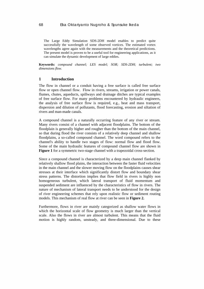
3.1 8Temporal Development of Horizontal Vortices The development of horizontal vortices can be described by using numerical computation as follow:

a. The longitudinal wavelength ( λ ) of vortices varies between 42 cm and 136 cm in statistical equilibrium. The result of this calculation is depicted on Figure 9 and 10.

b. The value of the wavelength ( λ ) both experiment and simulation are shown in Table 3. The mean value of the wavelength of the vortices predicted (simulation) at the observation point (at x=6400 cm, y=17 cm, as depicted on Figure 4) is 73.3 cm. The corresponding length was 76.9 cm, which agrees with the prediction. The calculation for finding the time period (T) of the wavelength (measurement) is done with Fast Fourier Transform (FFT). The result of spectrum graph is depicted in Figure 11.

c. Vorciticy field as shown in Figure 12, at several times, 10 st = , 30 st = , 60 st = , 90 st = , 120 s and 150 st = t = , indicating that small scale

horizontal vortices appear first and they grow by merging with each other. In the beginning flow, appears weak flow with the corresponding accumulation of vortices in five regions. After t = 90 s, the spatial pattern of vorticity has been found to reach an equilibrium state which the two large vortices formed.

-0.5

-0.4

-0.3

-0.2

-0.1

0

0.1

0.2

0.3

0.4

0.5

0 10 20 30 40 50 60 70 80 90 100 110 120 130 140 150

Time (sec)

η (m

m)

Figure 9 Variation of water surface elevation at measurement point, x=6400 cm and y=17 cm (numerical calculation).


Tabel 3 Comparison value of wavelength ( λ ).

u (m/s) Re Froude T (s) λ (m) Simulation 0.265 15887 0.345 2.77 0.733 Measured 0.297 17826 0.387 2.59 0.769

0

20

40

60

80

100

120

140

0 10 20 30 40 50 60 70 80 90 100 110 120 130 140 150

Time (sec)

λ (c

m)

Figure 10 Variation of wave length ( λ ) at measurement point, x=6400 cm and y=17 cm (numerical calculation).

f=0.39 s-1f=0.39 s-1

Figure 11 Result of FFT at measurement point, x=6400 cm and y=17 cm (from experiment data).


Figure 12 Temporal development of horizontal vortices; Spatial distribution vorticity at t=10 sec,30 sec, 60 sec, 90 sec, 120 sec and 150 sec.

Figure 13 Temporal development of horizontal vortices; Spatial distribution water surface η at t=10 sec, 30 sec, 60 sec, 90 sec, 120 sec and 150 sec.

y(m

) 0 .1

0 .2

0 .3

0 .4

y(m

) 0 .1

0 .2

0 .3

0 .4

y(m

) 0 .1

0 .2

0 .3

0 .4

y(m

) 0 .1

0 .2

0 .3

0 .4

y(m

) 0 .1

0 .2

0 .3

0 .4

x (m )

y(m

)

0 0 .2 0 .4 0 .6 0 .8 1 1 .2 1 .4 1 .6 1 .8 2

0 .1

0 .2

0 .3

0 .4

F lo wv o r: -4 .5 -4 -3 .5 -3 -2 .5 -2 -1 .5 -1 -0 .5

10

30

60

90

120

150

150

120

90

60

30

10

y(m

)

0

0 .1

0 .2

0 .3

0 .4

y(m

)

0

0 .1

0 .2

0 .3

0 .4

y(m

)

0

0 .1

0 .2

0 .3

0 .4

y(m

)

0

0 .1

0 .2

0 .3

0 .4

y(m

)

0

0 .1

0 .2

0 .3

0 .4

x (m )

y(m

)

0 0 .2 0 .4 0 .6 0 .8 1 1 .2 1 .4 1 .6 1 .8 20

0 .1

0 .2

0 .3

0 .4

F lo w

e ta : -0 .0 0 0 1 6 m -0 .0 0 0 1 2 m - 8 E - 0 5 m -4 E - 0 5 m -8 .1 3 1 5 2 E -2 0 4 E - 0 5 m 8 E -0 5 m 0 .0 0 0 1 2 mmeta: -0.00016m -0.00012m -8E-05m -4E-05m -8.13152E-20m 4E-05m 8E-05m 0.00012m


0

5

10

15

20

25

30

35

40

45

50

00.050.10.150.20.250.30.350.4 y (m)

(cm

/sec

)

ExperimentNumerical Simulation

main channel (Bm) = 0.24 m flood channel (Bf) = 0.16 m

Figure 14 Transverse profiles of mean velocity at x=6400 cm.

0

0.5

1

1.5

2

2.5

3

3.5

4

4.5

5

00.050.10.150.20.250.30.350.4 y (m)

stre

ss (g

/cm

/s2)

Reynolds Stress(Measurement)Large Scale (LS)SDS from subgrid scaleTotal Reynolds stress (LS+SDS)

main channel (Bm) = 0.24 m flood channel (Bf) = 0.16 m

Figure 15 Reynolds stress profiles at x = 6400 cm.


η (m

m)

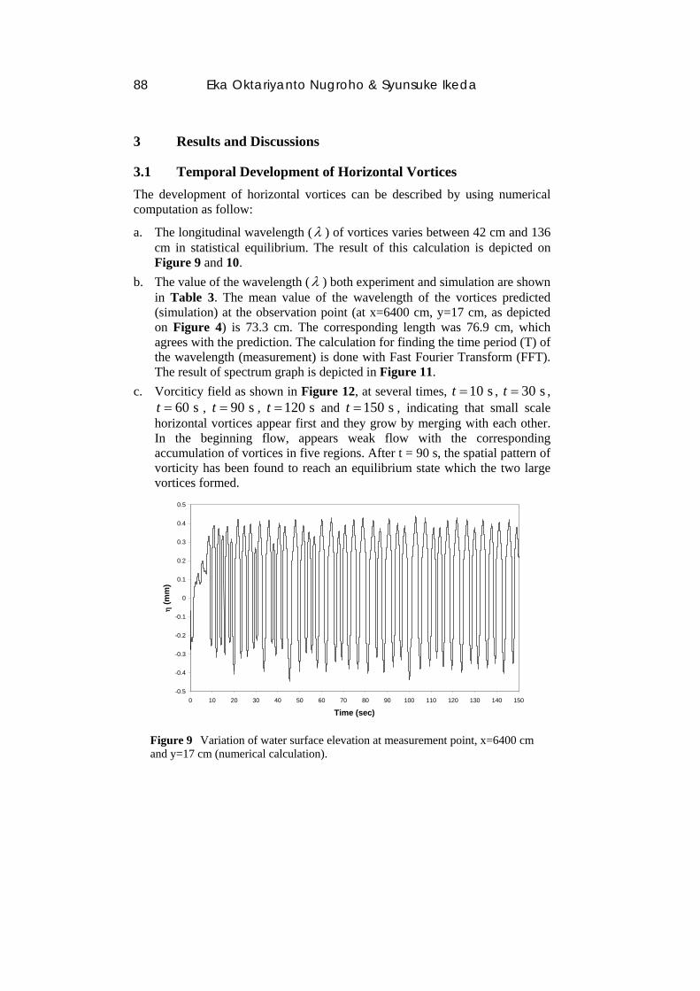
Figure 16 Temporal variation of free surface at x=6400 cm and y=17 cm (measured).

η (c

m)

Figure 17 Calculated variation of free surface at x=6400 cm and y=17 cm.

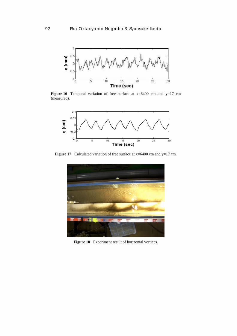
Figure 18 Experiment result of horizontal vortices.


Figure 19 Velocity with water surface contour.

Figure 20 Velocity with vorticity contour.

eta: -0.00016m -0.00012m -8E-05m -4E-05m -8.13152E-20m

3.2 9Instantaneous Flow Field The instantaneous 2D velocity with water surface contour and vorticity field are depicted in Figure 19 and 20, respectively, in which the velocity field is seen in the frame moving with the temporally averaged velocity at the boundary of the main channel and the flood channel (y = 16 cm). The maximum vorticity locates upstream of the geometrical center of the vortex. The vortices are inclined toward the longitudinal direction, which is important in producing the Reynolds stress.

The instantaneous free surface elevation calculated is shown in Figure 19, in which it is clear that the elevation is low near the center of the vortices. Figure 19 and 20 give comparison, which it is found that the regions with water surface depression nearly coincide with the central parts of horizontal vortices.

The variations of free surface elevation at y = 16 cm are depicted in Figure 16 and 17 for the measurement and prediction, respectively. The range of time is chosen for the 30 second in the end of calculation (It means from t=120 sec to 150 sec), with assumption that both of calculation and measurement are stable.

4E-05m 8E-05m 0.00012m

x (m)

y(m

)

0 0.2 0.4 0.6 0.8 1 1.2 1.4 1.6 1.8 2

0.1

0.2

0.3

0.4

0.3m/secFlow

vor: -4.5 -4 -3.5 -3 -2.5 -2 -1.5 -1 -0.5

x (m)

y(m

)

0 0.2 0.4 0.6 0.8 1 1.2 1.4 1.6 1.8 2

0.1

0.2

0.3

0.40.3m/secFlow


In the measurement graph, the range of the variation of height water surface and time period are similar. The calculation of time period gives the same result. Figure 18 and 20 give comparison the vorcity, it is found similar

3.3 1 0Temporally-Averaged Flow Field The lateral velocity distribution is shown in Figure 14. The agreement is reasonable. However, the measured values near y = 16 cm are a little smaller than the prediction, the reason for which is the existence of secondary flow which is fairly large near the boundary of the main channel and the flood plain. It transports near-bottom small fluid momentum toward the free surface, inducing small longitudinal flow velocity at around y = 20 cm. The present model cannot include the effect of secondary flow.

3.4 1 1Reynolds Stress The contribution of horizontal vortices shows the major part of the Reynolds stress as shown in Figure 14. Figure 14 shows the transverse distribution of the Reynolds stress (RS), there is a small difference between the computed maximum stress and the measured one, the profile of stress and the location of the maximum stress are similar. The Reynolds stress (Rs) is obtained from the sum of the stress from large-scale (LS) term and that from the subgrid scale (SDS). The large-scale is computed with the result of the computation while the subgrid scale is evaluated by the eddy-viscosity model with the SDS turbulent viscosity given by equation (22). The contribution of Reynolds stress from the explicitly computed large-scale (LS) eddies is larger than that from the modeled subgrid scale (SDS) eddies. The maximum of the Reynolds Stress occurs at the interface where the velocity gradient is the greatest.

4 5Conclusion A Large Eddy Simulation SDS-2DH model has been applied to study the lateral momentum transfer in compound channel which instantaneous structure of horizontal vortices and temporally-averaged velocity distribution have significant effect.

The results show the horizontal vortice occurs at the boundary between main channel and the flood channel where significant momentum exchange occurs.

The present model is proven to be a useful tool for engineering applications.


Acknowledgment Firstly, I would like to express my gratitude to Professor Syunsuke Ikeda. His supervision, support and patience were constant throughout this work and encouraged me to go on. My thanks go also to Dr. Akamatsu and Dr. Osawa. Their advices were very helpful and I benefited from their knowledge I am grateful to my sponsors, Tokyo Institute of Technology, on commission from the Ministry of Education, Culture, Sports, Science and Technology (MEXT), Japan, in collaboration with United Nations Educational, Scientific and Cultural Organization (UNESCO), who made this project viable.

Notations The following symbols are used in this paper: a = vegetation density parameter B = channel width Bf = flood channel width Bm = main channel width

bC = drag coefficient of vegetation

fC = bottom friction coefficient

Cμ = turbulence model parameter, a numerical constant

dC = turbulence model parameter, a numerical constant g = gravitational acceleration h = mean water depth H = total water column height (total depth) Hf = flood channel depth Hm = main channel depth ,i j = 1,2,3 and repeated indices show summation I = longitudinal channel bed slope l = length scale of SDS turbulence n = manning’s coefficient p = pressure

ap = pressure at the free surface

khp = energy production rate of turbulence due to horizontal shear

kvp = energy production rate of turbulence due to vertical shear/bottom friction

0S = longitudinal channel bed slope (x direction) t = time


u = depth averaged velocity in x direction u = mean or large scale velocity in x direction u′ = fluctuation or small scale/subgrid-scale velocity in x direction U = depth averaged velocity in x direction v = depth averaged velocity in y direction

v = mean or large scale velocity in y direction v′ = fluctuation or small scale/subgrid-scale velocity in y direction V = depth averaged velocity in x direction w = depth averaged velocity in direction zw = mean or large scale velocity in z direction w′ = fluctuation or small scale/subgrid-scale velocity in z direction , , x y z = longitudinal, transverse and vertical coordinate, respectively

ix = Cartesian coordinates, , x y and zα = a numerical constant β = Boussinesq coefficient δij = Kronecker ε = dissipation rate of kinetic energy η = water surface displacement λ = wave length μ = dynamic viscosity ρ = water density

kσ = a numerical constant

tυ = eddy viscosity

bxτ = bottom shear stress in x direction

byτ = bottom shear stress in y direction

References [1] Shiono, K., & Knight, D.W., Turbulent Open-Channel Flows with

Variable Depth Across the Channel, Journal of Fluid Mechanics, 222, 617-646, 1991.

[2] Tuitoek, D. K., Coupled Equations for Modeling Unsteady Flow in Channels with Floodplains, Thesis for Doctor’s Degree, Department Civil and Environmental Engineering, Faculty of Engineering, University of Alberta, Canada, 1995.

[3] Deardorf, J.W., A Numerical Study of Three-Dimensional Turbulent Channel Flow at Large Reynolds Numbers, Journal Fluid Mech., Cambridge, England, UK, 41, 453-480, 1970.


[4] Leonard, A., On The Energy Cascade in Large-Eddy Simulations of Turbulent Fluid Flows, Technical Report Rep. TF-1, Thermosciences Div., Stanford University, Dept. Mech. Eng., Stanford, CA 94305, California, 1973.

[5] Ikeda, S., Hydraulics, Gijyutsudou Syuppan, Tokyo (In Japanese), 1999. [6] Salvetti, M. V., & Banerjee, S., A Priori Tests of a New Dynamic

Subgrid-Scale Model for Finite-Difference Large Eddy Simulations, Phys. Fluids, 7 (11), 1995.

[7] Worthy, J., Large Eddy Simulation of Buoyant Plumes, Thesis for Doctor’s Degree, School of Mechanical Engineering, Cranfield University, 2003.

[8] Nadaoka, K. & Yagi, H., Shallow Water Turbulence Modeling and Horizontal Large-Eddy Computation of River Flow, Journal of Hydraulic Engineering, ASCE, 124(5), 493-500, 1998.

[9] Ikeda, S., Ohta K., & Hasegawa, H., Instability-Induced Horizontal Vortices in Shallow Open-Channel Flows with an Inflection Point in Skewed Velocity Profile, J. Hydroscience and Hydraulic Engineering Tech., Japan Society of Civil Engineers, 12(2), 69-84, 1994.

[10] Rastogi, A.K., & Rodi, W., Predictions of Heat and Mass Transfer in Open Channels, Journal of the Hydraulics Division, ASCE, 104(3), 397-420, 1978.

[11] McKibben , J.F., A Computational Fluid Dynamics Model for Transient Three-Dimensional Free Surface Flows, Thesis for Doctor’s Degree, Institute of Paper Science and Technology, Atlanta, Georgia, 1993.

[12] Bousmar, D., Flow Modelling in Compound Channels, Momentum Transfer between Main Channel and Prismatic or Non-Prismatic Floodplains, Thesis for Doctor’s Degree, Faculté des Sciences Appliquées, Unité de Génie Civil et Environemental, Université catholique de Louvain, France, 2002.

[13] Ikeda, S., Invited Lecture: Role of Lateral Eddies in Sediment Transport and Channel Formation, River Sedimentation, Jayawardena, Lee & Wang, eds., Balkema, Rotterdam, 195-205, 1999.

[14] Ikeda, S., et al, Large Eddy Simulation of Flow and Sediment Transport in Compound Channels, 3rd Int. Symposium on Turbulence, Heat and Mass Transfer, Tokyo, Japan, 2000.

[15] Nugroho, Eka, O., & Ikeda, S., Application Large Eddy Simulation SDS-2DH Model to Flow in A Compound Channel, Working Report, Tokyo Institute of Technology-UNESCO International Research Course for the Environment, 2006.

[16] Rodi, W., Turbulence Models and Their Application in Hydraulics: A State of The Art Review, IAHR book publications, Delft, 1980.

comparison study of flow in a compound channel

Documents