HAL Id: ujm-00461006https://hal-ujm.archives-ouvertes.fr/ujm-00461006

Submitted on 30 May 2016

HAL is a multi-disciplinary open accessarchive for the deposit and dissemination of sci-entific research documents, whether they are pub-lished or not. The documents may come fromteaching and research institutions in France orabroad, or from public or private research centers.

L’archive ouverte pluridisciplinaire HAL, estdestinée au dépôt et à la diffusion de documentsscientifiques de niveau recherche, publiés ou non,émanant des établissements d’enseignement et derecherche français ou étrangers, des laboratoirespublics ou privés.

Comparison of the efficiency, MTF and chromaticproperties of four diffractive bifocal intraocular lens

designsFannie Castignoles, Manuel Flury, Thierry Lépine

To cite this version:Fannie Castignoles, Manuel Flury, Thierry Lépine. Comparison of the efficiency, MTF and chromaticproperties of four diffractive bifocal intraocular lens designs. Optics Express, Optical Society ofAmerica, 2010, 18 (5), pp.5245-5256. <10.1364/OE.18.005245>. <ujm-00461006>

Comparison of the efficiency, MTF and

chromatic properties of four diffractive bifocal

intraocular lens designs

Fannie Castignoles 1*, Manuel Flury

1, and Thierry Lepine

1,2

1Université de Lyon, F-42023, Saint-Etienne, France;

CNRS, UMR 5516, Laboratoire Hubert Curien, F-42000, Saint-Etienne, France;

Université de Saint-Etienne, Jean-Monnet, F-42000, Saint-Etienne, France 2Institut d'Optique Rhône-Alpes 18 rue Benoît Lauras F-42000 Saint-Etienne, France

*fannie.castignoles@univ-st-etienne.fr

Abstract: The aim of this paper is to compare the properties of four

different profiles which can be used as multifocal intraocular lens. The

Hankel transform based on the theory of scalar diffraction is applied to a

binary profile, a parabolic one, a parabolic profile with holes, and finally a

sinusoidal one. This enables to study the various distributions of the

diffractive efficiencies and the axial chromatism. The image quality is

evaluated by means of simulations of the MTFs with Zemax®. Finally we

propose a new way to graphically synthesize all the properties of these

lenses, using a radar graph.

References and links

1. J. A. Davison, and M. J. Simpson, “History and development of the apodized diffractive intraocular lens,” J.

Cataract Refract. Surg. 32(5), 849–858 (2006).

2. A. L. Cohen, “Diffractive bifocal lens designs,” Optom. Vis. Sci. 6, 461–468 (1993).

3. V. Moreno, J. F. Roman, and J. R. Salguerio, “High efficiency diffractive lenses: Deduction of kinoform

profile,” Am. J. Phys. 65(6), 556–562 (1997).

4. B. Kress, and P. Meyrueis, Digital Diffractive Optics: An introduction to planar diffractive optics and related

technology (John Wiley and Sons, 2000).

5. D. Baude, PhD-thesis, “Caractérisation, optimisation et réalisation de composants optiques multifocaux

diffractifs et réfractifs,” Université Paris-Sud, centre d’Orsay, France (1990).

6. A. L. Cohen, “Progressive intensity phase bifocal,” US patent application 438,320 (November 1989).

7. M. Guizar-Sicairos, and J. C. Gutiérrez-Vega, “Computation of quasi-discrete Hankel transforms of integer order

for propagating optical wave fields,” J. Opt. Soc. Am. A 21(1), 53 (2004).

8. A. Lang, and V. Portney, “Interpreting multifocal intraocular lens modulation transfer functions,” J. Cataract

Refract. Surg. 19(4), 505–512 (1993).

9. A. L. Cohen, “Diffraction bifocal with adjusted chromaticity,” US patent application 553,336 (July 1990).

10. A. L. Cohen, “Diffractive multifocal optical device,” US patent application 456,226 (December 1989).

11. L. N. Thibos, M. Ye, X. Zhang, and A. Bradley, “The chromatic eye: a new reduced-eye model of ocular

chromatic aberration in humans,” Appl. Opt. 31(19), 3594–3600 (1992).

1. Introduction

Multifocal intraocular lenses are nowadays widely used in the correction of presbyopia,

offering the pseudophakic patient far and near vision with one implant [1].

The profile of such bifocal diffractive lenses can be binary or continuous with various

forms (parabolic, hyperbolic, sinusoidal…). This profile will determine the optical properties

of the lens, notably in terms of efficiency, MTF (modulation transfer function) and

chromatism.

In the present manuscript we will study four important multifocal diffractive profiles (a

parabolic one, a parabolic profile with holes, a sinusoidal one and a binary one) with a

common addition of + 3 dioptres ( + 3 D is the power of the IOL lens which corresponds to an

equivalent of + 2.4D of glass addition), and we will compare their properties in a radar graph

that highlights their respective characteristics.

The first criterion retained for this study is the diffractive efficiency at 550 nm, which will

be obtained with a Hankel transform of the profile at stake. In a second part, a simplified

model in Zemax® is employed to compare the MTF of the near and the far focus, at 550 nm.

Eventually in a third part, the diffractive efficiency and the MTF at 440 nm and 640 nm are

calculated, shedding light on the effects of chromatism due to the different profiles. All theses

data are then gathered in a single figure in part 6.

2. Description of the lenses designs

Multifocal intraocular lenses used to correct presbyopia are made of a carrier lens which

determines the power for the far vision of the bifocal, whereas the diffractive profile provides

the added power (used to correct the near vision) [2]. In this paper we will only study planar

lenses in order to focus on the addition of power and the bifocality provided by the diffractive

profile. This work can be easily transposed to a curved IOL, if the diffractive orders are

moved on the power scale according to the refractive power added to the base of the lens.

All the lenses studied in this paper have a diameter of 3 mm, corresponding to the average

diameter for eye pupils in photopic light. The choice of the addition is + 3D which

corresponds to a focal length of 333 mm. The radii of the annular concentric zones depend on

the focal length. In a parabolic profile, a parabolic profile with holes, and a sinusoidal one the

rings are spaced according to the formula [3]:

( ) 2R k k f λ= ⋅ ⋅ ⋅ (1)

where R (k) is the zone radii and k is the integer which corresponds to the kth

zone.

Otherwise in the binary profile which consists of full and empty zones, the radii of the full

zones are equal to [3]:

( )' ,R k k f k oddλ= ⋅ ⋅ (2)

Thus the parabolic, parabolic with holes, and sinusoidal lenses with a 3 mm diameter

contain 6 annular concentric zones, and the binary profile contains 6 empty and 6 full zones.

In order to have a bifocal lens which divides light fairly equally between the two images, the

steps of the diffractive profile must delay light of ½ wavelength [2,3]. The height of the steps

is equal to:

max

0.5h

n

λ⋅=∆

(3)

where ∆n is the difference in the refractive index between the lens and its environment, and λ

is the design wavelength of the lens (here λ = 550 nm).

However an exception is made to the sinusoidal profile, which needs a maximum height

of:

'

max

0.415h

n

λ⋅=

∆(4)

to become bifocal with the same efficiency in the near and far focus [2]. The four different

profiles examined in this paper are represented in Fig. 1.

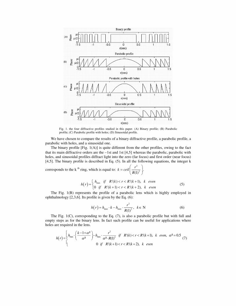
Fig. 1. the four diffractive profiles studied in this paper. (A) Binary profile; (B) Parabolic

profile; (C) Parabolic profile with holes; (D) Sinusoidal profile.

We have chosen to compare the results of a binary diffractive profile, a parabolic profile, a

parabolic with holes, and a sinusoidal one.

The binary profile [Fig. 1(A)] is quite different from the other profiles, owing to the fact

that its main diffractive orders are the −1st and 1st [4,5] whereas the parabolic, parabolic with

holes, and sinusoidal profiles diffract light into the zero (far focus) and first order (near focus)

[4,5]. The binary profile is described in Eq. (5). In all the following equations, the integer k

corresponds to the k th

ring, which is equal to: 2

2(1)

rk ceil

R

=

.

( ) max '( ) '( 1),

0 '( 1) '( 2),

h if R k r R k k evenh r

if R k r R k k even

< < +=

+ < < +(5)

The Fig. 1(B) represents the profile of a parabolic lens which is highly employed in

ophthalmology [2,3,6]. Its profile is given by the Eq. (6):

( )2

max max 2,

(1)

rh r h k h k

R= ⋅ − ⋅ ∈Ν (6)

The Fig. 1(C), corresponding to the Eq. (7), is also a parabolic profile but with full and

empty steps as for the binary lens. In fact such profile can be useful for applications where

holes are required in the lens.

( )

2

max max 2

1 ²'( ) '( 1), , ² 0.5

² ² (1)

0 '( 1) '( 2),

k rh h if R k r R k k even

h r R

if R k r R k k even

αα

α α − + ⋅ − ⋅ < < + = = ⋅ + < < +

(7)

The last profile, Fig. 1(D) and Eq. (8) is sinusoidal, and can be employed in some

applications instead of the parabolic one. In particular, a sinusoidal profile advantageously

exhibits thinner and smoother steps [2,6].

( )' 2

max

21 ( 1) cos( )

2 (1)

kh rh r

Rπ

= ⋅ − − ⋅ ⋅

(8)

3. Diffractive efficiencies at 550 nm

3.1. Methods

One way to calculate the diffractive efficiencies is to use a Fourier transform [5]. In fact when

the transmission function t is periodic in r2, it can be expressed as a Fourier sum:

( ) ²exp 2 .

(1)²p

p Z

rt r C i p

Rπ

∈

= ⋅

∑ (9)

where R(1) is the period of the function t in the r2 space and the

pC are the coefficients given

by:

(1)²

0

1( )exp 2

(1)² (1)²

R

p

uC t r i p du

R Rπ

= − ⋅ ⋅

∫ (10)

The diffractive efficiency pη of each order p will be the squared modulus of its

coefficient in the Fourier series of the transmission function t:

²p pCη = (11)

However, even if the Fourier transform is a rapid and useful tool to calculate the

efficiencies of a diffractive lens, it is limited to transmission functions periodic in the r2 space,

which is not always the case. For instance sawtooth profiles cannot be described with the

Fourier transform. Moreover the pupil is not taken into account in this method.

That is why another method based on wave propagation is employed. This method is

based on the theory of scalar diffraction and allows the efficiency of each kind of design to be

calculated. Moreover the propagation of the field can be studied and represented, which is of

interest to observe the variation of focal length of our systems.

This wave propagation is numerically implemented in Matlab, as is described in reference

[7]. Quasi-discrete Hankel transform of the 0 order is used to adapt the circularly symmetric

function of the different transmission functions.

The lens is normally illuminated with an incident plane wave.

The efficiencies of the convergent orders (negatives orders in our convention) are

calculated from the square modulus of the field. Thus for each order the energy contained in

the first ring of the corresponding Airy pattern (at the focal plane and its fractions f/2, f/3 …)

corresponds to 84% of the diffractive efficiency in this order.

The efficiencies of the divergent orders (positives ones), are calculated in the same way,

applying the Hankel transform to the complementary phase of the diffractive lens.

Finally the calculation of the zero-order efficiency requires the use of an additional perfect

refractive lens to determine the efficiency of the diffractive lens in its focal plane.

3.2. Results

Fig. 2. Distribution of the diffractive efficiencies at 550 nm for the four different lenses. (A)

Parabolic profile; (B) Parabolic profile with holes; (C) Sinusoidal profile; (D) Binary profile

In Fig. 2 are represented the distributions of the diffractive efficiencies between the orders −2to + 2, for each of the four profiles described in Fig. 1. The total efficiencies plotted in Fig. 2

do not add to 100% because the orders greater than +/−2 have finite but small efficiencies too.

As it was explained previously, the diffractive efficiency of the binary profile [Fig. 2(D)]

is shared between the −1st and 1st order with about 37% of efficiency. Moreover there is no

efficiency for the even orders which is a characteristic of binary diffractive lenses. The

diffractive efficiencies of the parabolic profile [Fig. 2(A)] are about 40% but affect the −1st

and 0th orders. Furthermore its −2nd and 1st orders have a non negligible efficiency of about

5%. The parabolic profile with holes [Fig. 2(B)], has slightly lower diffractive efficiencies in

the −1st and 0th order compare to the parabolic lens. It has also a non negligible efficiency in

the −2nd and 1st orders (reaching 10%), which can lead to halos. The sinusoidal profile

[Fig. 2(C)], keeps diffractive efficiencies close to 40% in the −1st and 0th orders, but exhibits

also quite important efficiency in the first order.

4. Simulation of the MTF at 550 nm

A second performance characteristic of the different profiles is the modulation transfer

function, which provides the spatial frequency response of the imaging system [8]. The MTFs

are calculated with Zemax®, which is a software used to design optical systems and perform

optical simulations. The four diffractive lenses are created from their radial coordinates

inserted in a .TOB file in Zemax®. The resulting non sequential objects are then inserted in a

very simplified model of the eye described in Fig. 3.This optical system allows to simulate

the MTF at the focal plane of the eye, for both a near and a far object.

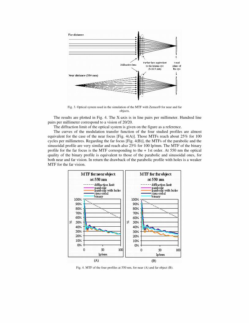
Fig. 3. Optical system used in the simulation of the MTF with Zemax® for near and far

objects.

The results are plotted in Fig. 4. The X-axis is in line pairs per millimeter. Hundred line

pairs per millimeter correspond to a vision of 20/20.

The diffraction limit of the optical system is given on the figure as a reference.

The curves of the modulation transfer function of the four studied profiles are almost

equivalent for the case of the near focus [Fig. 4(A)]. Those MTFs reach about 25% for 100

cycles per millimetres. Regarding the far focus [Fig. 4(B)], the MTFs of the parabolic and the

sinusoidal profile are very similar and reach also 25% for 100 lp/mm. The MTF of the binary

profile for the far focus is the MTF corresponding to the + 1st order. At 550 nm the optical

quality of the binary profile is equivalent to those of the parabolic and sinusoidal ones, for

both near and far vision. In return the drawback of the parabolic profile with holes is a weaker

MTF for the far vision.

Fig. 4. MTF of the four profiles at 550 nm, for near (A) and far object (B).

5. Effects of chromatism

5.1. Introduction

An important drawback of a diffractive lens is its wavelength dependency [5,9]. In fact the

wavelength plays directly a part in the radius of the circular rings [Eq. (1), (2)], and in the

height of those rings [Eq. (3), (4)]. Moreover the variation of λ implies also a variation of the

refractive index n, which in its turn causes a modification of the radius and height of the rings.

However, this dispersion of the material n (λ) is insignificant compared to the variation of λ

itself. For example, with Polycarbonate (a very dispersive material with νd = 30) in air, and

for λ varying from 440 nm (blue) to 640 nm (red), d n

n

∆

∆is negligible compared to

dλλ

[Eq. (12), (13)]. However this is true for materials in air, but can be false for multilayer

components where d n

n

∆

∆may become important.

640 4400.364

550

dλλ

−= = (12)

[ ] [ ][ ]

(640) (440) (1.581 1.610)0.049

(550) 1.590 1

air air

air

n n n nd n

n n n

− − −∆ −= = =

∆ − − (13)

The variations of the radii and the height of the rings have an impact on the focal length

and the optical power of the lens, on the diffractive efficiencies and on the MTFs. These

produced modifications are compared in this paragraph for the four different profiles. The

results are calculated at 440 nm (blue), 550 nm (design wavelength) and 640 nm (red), using

the Hankel transform and Zemax® as it was described before.

5.2. Effects of chromatism on the focal length and the optical power

Given that the focal length is linked to the radii of the annular zones [Eq. (1), (2)], the

variation of λ will have an effect on f and as a direct consequence on the optical power of the

lens [9]:

0

0

PP P P

λ λλ λ⋅ ∆

= ⇒ ∆ = ⋅ (14)

According to the Eq. (14), the variation of the power of the lens between blue and red

(Table 1) depends only on the value of the power for the calculated order. We can thus

calculate ∆P for the first convergent order (−1st) which will be the same for the four profiles

studied here:

Table 1. Variation of the convergent focal length with wavelength.

λ (nm) Focal length (mm)

of the −1st order

Optical power (dioptres)

440 416 2.404

550 333 3.0

640 286 3.496

Thus the power deviation equals: ∆P = P red – P blue = 3.496-2.404 = 1.09 D, where P red is

the power of the lens for red light and P blue the power for blue light. ∆P is positive which is

characteristic of diffractive convergent components.

Besides, the variation in power for the higher convergent orders will increase

proportionally to the power. Thus, ∆P corresponding to the −2nd order will be twice as high

as ∆P for the −1st one. However in the case of the parabolic, parabolic with holes, and

sinusoidal profiles studied in this paper, the near focus is given by the first negative order, and

higher orders will thus not be considered.

Noteworthy, the far vision provided with the 0th order has no variation in its focal length

(infinite) caused by chromatic effects.

In return the two orders (−1st and 1st) used for near and far visions with the binary profile

suffer from chromatic effects. Furthermore, the positions of the red and blue foci for the far

vision ( + 1st divergent order) will be the opposite of the near foci ones, so that the binary

profile displays the disadvantage of being added to the chromatism of the human eye [10,11].

5.3. Effects of chromatism on the distribution of the diffractive efficiencies

The change in the phase difference with λ will lead to a variation of the distribution of the

efficiencies, and the MTFs.

Thus the variations of the diffractive efficiencies of the two interesting orders for each

profile are plotted versus λ in Fig. 5 . They are calculated with the Hankel transform.

Fig. 5. Variations of the diffractive efficiencies versus λ

The three parabolic, parabolic with holes, and sinusoidal profiles studied here behave the

same way, so that the convergent −1st order decreases with λ, whereas the 0th order rises.

Near 550 nm those two orders cross each other and reach about 40% of efficiency for the

parabolic and the sinusoidal profile, and about 35% for the parabolic profile with holes. This

latter has lower efficiencies throughout the curve. At 440 nm the three profiles proposed here

are much more efficient for the near vision. On the contrary, at 640 nm, the dominant order is

the far vision one.

The binary profile has a very different behavior, given that the −1st and + 1st orders have

the same variation of efficiency with λ. Moreover this variation is much weaker than the

other. Regarding the efficiencies’ variations with λ, the binary profile is much more balanced

than the others. This phenomenon can be intuitively understood since the complementary

form of a binary lens is also a binary lens. This complementarity explains the balanced results

between the positive and negative orders, whatever the wavelength.

5.4. Effects of chromatism on the MTFs

The impact of a wavelength change is also high in the MTFs (Fig. 6). First, the MTFs are now

calculated in the focus corresponding to the blue and red foci. Moreover, the variation of the

diffractive efficiencies has positive or negative impacts on the MTFs. In fact, the behavior of

the MTFs is directly linked to the variations of efficiency. Thus the higher the diffractive

efficiency is, the better the MTF curve will be. This is due to the fact that higher diffractive

efficiency in a useful order means lower stray light, and thus less contrast lost.

Thus the phenomena observed with the variations of efficiency are similar for the MTFs.

Indeed whereas the MTFs in blue and red for the binary profile are similar, it is obvious that

the parabolic, parabolic with holes, and sinusoidal profile’s MTFs are not balanced. Whereas

in blue light the near vision becomes strongly better than for the binary profile, the situation is

reversed in red light. On the contrary the MTF of the binary profile is higher than the three

other profiles’ MTFs for the far object in blue, and inversely in red light.

Fig. 6. MTFs for the near and far vision, at 440 nm and 640 nm.

6. Synthesis of the different properties of each profile in a radar graph

In order to collect all the data previously obtained, a new way of illustrating the different

properties of each profile was employed in a “radar-type” graph (Fig. 7). The diffractive

efficiencies at 440 nm, 550 nm and 640 nm are plotted for the two useful orders. Besides

punctual data on the MTF curves representative of the quality of the vision have to be

selected. Thus the values of the MTF for near and far objects have been plotted at a frequency

of 100 lp/mm, which corresponds to a visual acuity of 20/20. Furthermore it is interesting to

represent the properties for the near vision in front of those of the far one. This underlines the

symmetry of the results of the binary profile for near and far vision, contrary to the

dissymmetry of the parabolic, parabolic with holes, and sinusoidal profiles behaviors.

Fig. 7. radar graphs for the four different profiles.

Advantages and drawbacks of each design can be assessed by the superimposition of those

figures in a same graph (Fig. 8). The choice of the profile will then depends on the specific

needs of the designer. For instance the use of a binary profile can be interesting for a bifocal

lens requiring two balanced diffractive orders, and a small dependence with λ. Otherwise the

superimposition of the merit figures for the parabolic and the sinusoidal designs highlights the

similarity of their results. In return, the inclusion of the figure for the parabolic profile with

holes inside the parabolic and sinusoidal profiles figures shows that only diffractive lenses

that absolutely require holes can take advantage out of it.

Fig. 8. Superimposition of the radar graphs for the four different profiles.

7. Conclusion

This paper provides a study of the properties of four designs that can be used for multifocal

diffractive lenses with a view to correcting presbyopia.

The binary profile, which diffracts light into the −1st and + 1st order, and the parabolic

one, often used in diffractive IOL are well known in the art. The third one, a sinusoidal profile

is sometimes used as a variant of the parabolic one. The study of the distribution of the

diffractive efficiencies and the MTFs for several wavelengths shows that those two latter

profiles exhibit very similar behaviors. On the contrary, the binary profile gives quite

different results. Indeed its symmetric behavior leads to two main orders very balanced and

less wavelength dependent. However other criterion like the sign of its chromatism must be

considered before use. Besides, an intermediate design made of a parabolic profile with holes

(like the binary one) has been compared to the previous ones. The results obtained with the

Hankel transform and the Zemax® simulations show a slightly lower efficiency and MTF

compared to the other profiles. It can still be used in a system where holes are needed.

Finally a radar graph (Fig. 8) is proposed to better comprehend the different parameters

involved in the choice of a specific profile. This graph takes into account the distribution of

efficiencies of the two main diffractive orders at 440 nm, 550 nm, and 640 nm and draws a

parallel with the corresponding MTFs which illustrates the variation in image quality.

However although this radar graph consists in a useful tool, the choice of a profile should also

take into account the fabrication technology. For instance the choice of a binary lithography

technology will be more appropriated for a binary profile, whereas the use of diamond tool or

grey-tone lithography enables to design continuous profiles. Other parameters like

geometrical constraints of the lens may also play a role in the choice of the profile.

Acknowledgements

The authors wish to thank G. Cohen and P. Chavel for their helpful discussions and the

National Association for Research and Technology (ANRT) for its financial support.