comparison of the device lifetime in wireless networks for

HAL Id: hal-01649135https://hal.archives-ouvertes.fr/hal-01649135

Submitted on 27 Nov 2017

HAL is a multi-disciplinary open accessarchive for the deposit and dissemination of sci-entific research documents, whether they are pub-lished or not. The documents may come fromteaching and research institutions in France orabroad, or from public or private research centers.

L’archive ouverte pluridisciplinaire HAL, estdestinée au dépôt et à la diffusion de documentsscientifiques de niveau recherche, publiés ou non,émanant des établissements d’enseignement et derecherche français ou étrangers, des laboratoirespublics ou privés.

Comparison of the Device Lifetime in Wireless Networksfor the Internet of Things

Elodie Morin, Mickael Maman, Roberto Guizzetti, Andrzej Duda

To cite this version:Elodie Morin, Mickael Maman, Roberto Guizzetti, Andrzej Duda. Comparison of the Device Life-time in Wireless Networks for the Internet of Things. IEEE Access, IEEE, 2017, 5, pp.7097 - 7114.�10.1109/ACCESS.2017.2688279�. �hal-01649135�

https://hal.archives-ouvertes.fr/hal-01649135

https://hal.archives-ouvertes.fr

Received January 24, 2017, accepted March 1, 2017, date of publication April 7, 2017, date of current version June 7, 2017.

Digital Object Identifier 10.1109/ACCESS.2017.2688279

Comparison of the Device Lifetime in WirelessNetworks for the Internet of ThingsÉLODIE MORIN1,2,3, MICKAEL MAMAN2, ROBERTO GUIZZETTI1,AND ANDRZEJ DUDA3, (Member, IEEE)1STMicroelectronics, 38140 Crolles, France2CEA-LETI, MINATEC, 38000 Grenoble, France3CNRS Grenoble Informatics Laboratory, Grenoble Institute of Technology, Grenoble Alps University, 38000 Grenoble, France

Corresponding author: Élodie Morin ([email protected])

This work was supported in part by the French Ministry of Research projects DataTweet under Contract ANR-13-INFR-0008-01 and inpart by the PERSYVAL-Laboratory under Contract ANR-11-LABX-0025-01.

ABSTRACT This paper presents a comparison of the expected lifetime for Internet of Things (IoT) devicesoperating in several wireless networks: the IEEE 802.15.4/e, Bluetooth low energy (BLE), the IEEE 802.11power saving mode, the IEEE 802.11ah, and in new emerging long-range technologies, such as LoRa andSIGFOX. To compare all technologies on an equal basis, we have developed an analyzer that computes theenergy consumption for a given protocol based on the power required in a given state (Sleep, Idle, Tx, and Rx)and the duration of each state. We consider the case of an energy constrained node that uploads data to a sink,analyzing the physical (PHY) layer under medium access control (MAC) constraints, and assuming IPv6traffic whenever possible. This paper considers the energy spent in retransmissions due to corrupted framesand collisions as well as the impact of imperfect clocks. The comparison shows that the BLE offers the bestlifetime for all traffic intensities in its capacity range. LoRa achieves long lifetimes behind 802.15.4 and BLEfor ultra low traffic intensity; SIGFOX only matches LoRa for very small data sizes. Moreover, consideringthe energy consumption due to retransmissions of lost data packets only decreases the lifetimes withoutchanging their relative ranking. We believe that these comparisons will give all users of IoT technologiesindications about the technology that best fits their needs from the energy consumption point of view. Ouranalyzer will also help IoT network designers to select the right MAC parameters to optimize the energyconsumption for a given application.

INDEX TERMS Internet of Things (IoT), wireless sensor networks, 6LoWPAN, 802.15.4e, TSCH,802.11ah, Bluetooth low energy, LoRa, SIGFOX, energy consumption model, clock drift.

I. INTRODUCTIONThe Internet of Things (IoT) aims at connecting small con-strained devices to the Internet via the IP protocol, whichenables new communicating applications. Ultra low energyconsumption is critical for IoT devices since they mostlyoperate on batteries and they need to reach lifetimes ofthe order of several years without battery replacement. Lowpower operation becomes even more challenging for nodesthat harvest energy from the environment, for instance usingsolar panels. They can only consume a small amount ofenergy over short time intervals that needs to be compensatedby energy intake. An estimation of the energy consumptionand the device lifetime is thus crucial for choosing the mostappropriate technology and finding the optimal settings ofconfiguration parameters.

Until recently, ultra low-power devicesmainly relied on the802.15.4 standard [1] that was specifically designed for low

energy consumption. However, the work by Tozlu [2] showedthat some 802.11 devices can also benefit from good energyefficiency in 802.11b Power Saving Mode (PSM) [3] andeven outperform 802.15.4. Bluetooth Low Energy (BLE) [4]has also added another competitor to the low-power stan-dards, and besides the short-range solutions, emerging long-range technologies such as 802.11ah [5], LoRa [6], andSIGFOX [7] also aim at high energy efficiency.

In this paper, we present a comparison of the expected life-time for IoT devices operating in the wireless networks listedin Table 1: beacon-enabled IEEE 802.15.4, the Time SlottedChannel Hopping (TSCH) variant of IEEE 802.15.4e [8],Bluetooth Low Energy (BLE), IEEE 802.11 PSM, and futureIEEE 802.11ah. We also consider the emerging long-rangetechnologies (LoRa and SIGFOX) to see how they performcompared to other protocols. We assume IPv6/6LoWPANprotocols whenever possible (see Fig. 1) and carefully

VOLUME 5, 20172169-3536 2017 IEEE. Translations and content mining are permitted for academic research only.

Personal use is also permitted, but republication/redistribution requires IEEE permission.See http://www.ieee.org/publications_standards/publications/rights/index.html for more information.

7097

É. Morin et al.: Comparison of the Device Lifetime in Wireless Networks for IoT

TABLE 1. Overview of the analyzed technologies.

FIGURE 1. Protocol stack of the considered technologies.

analyze the energy consumption patterns for duty-cycledMAC layers to derive the lifetimes.

A. MOTIVATION AND RESEARCH GOALSThemotivation for this paper comes from the observation thatmany different wireless technologies can be used for IoT andthere is no exhaustive comparison in the literature of theirenergy consumption that would help to make right decisionabout deployment of a given network. Although some char-acteristics of the considered technologies, such as the rangeor the used bandwidth, are not directly comparable, there isa need for a thorough comparison of the energy efficiencyto identify their key factors and limitations. Many overviewsof different wireless networks exist [9]–[13], but to the bestof our knowledge, no previous work compares a large set ofwireless networks for IoT from the energy efficiency pointof view while setting them on an equal basis. Some papersjust study two technologies [14], [15], but a comparison withother possible solutions is still missing. Such a comparisonwith all technologies laid on the same basis can bring tolight the respective advantages and drawbacks to drive thefuture developments for improving performance and energyconsumption.

Another motivation of our work is to extend the energyconsumption models that reflect the operation of duty-cycledMAC layers, which is often neglected in energy consumptionstudies. Before recent papers that set the principles of theenergy model we use [16]–[18], energy consumption modelsonly took into account the following main aspects: transmis-sion power, distance between two nodes, packet size, andpath loss [19]–[23]. This approach onlymodeled the behaviorof the physical layer and it did not reflect the operation of

duty-cycled IoT devices in a realistic way. Our goal was toextend the recent realistic energy consumption models to allconsidered technologies and make them available through anopen source tool allowing anybody to play with the networkparameters and quickly estimate lifetimes.

Finally, we want to evaluate the impact of pushing the IPprotocols to constrained IoT devices by taking into accountnot only the hardware performance and duty-cycled MACoperation, but also the protocol overhead (headers and frag-mentation), along with the cost of keeping an active connec-tion and time synchronization between two nodes. In this way,we can evaluate the impact of all layers on energy consump-tion and performance. The overall goal of this paper is to helpall users of IoT technologies to choose the technology thatbest fits their needs from the perspective of energy efficiency.

B. ASSUMPTIONS, RESEARCH METHOD,AND CONTRIBUTIONWe consider the case of an energy constrained node (battery-operated or energy harvesting) that generates and uploadsdata to a sink (uplink traffic). We adopt the view of an IoTdevice that connects to the network and wants to stay alivefor the longest time. We limit the scope of the paper to asingle link case, because it is the current most common con-figuration setup, a kind of a baseline for comparisons (notethat many papers limit the scope to a single link case, e.g. theanalytical energy consumption model of B-MAC proposedby Polastre et al. [24]). Moreover, the topology of all theconsidered networks except 802.15.4 is a star one in whicha node connects to or associates with a main-powered nodeto obtain Internet connectivity. In the future work, we planto extend the analysis to multi-hop 802.15.4 and upcomingmesh BLE networks.

Our research method consists of analyzing energyconsumption of each technology by considering a real-istic energy model in which the main energy con-sumers (radio transceiver, microcontroller) alternate betweenactive and inactive states (Tx, Rx, Idle, Sleep) withknown power consumption patterns and timing con-straints defined by the MAC layers. We derive the modelfrom the previous proposals for 802.15.4/e [16]–[18],extend them to other MAC technologies, and use it to analyzethe technologies in function of different parameters.

For the presented analysis, we assume the applicationtraffic workload composed of variable UDP (User DatagramProtocol) packet sizes over IPv6/6LoWPAN protocols when-ever possible (see Fig. 1) or over a given MAC layer oth-erwise. The analysis takes into account the energy spentin data frame retransmissions due to corrupted frames andcollisions. We consider the energy consumption for differenthardware platform parameters (i.e. energy consumption perstate) to find the parameters resulting in the minimal energyconsumption. We then adopt the minimal energy hardwareplatforms to compute the lifetime of the considered technolo-gies for application trafficwith varying intensity, Packet ErrorRate (PER), and clock precision. The premise is that even if

7098 VOLUME 5, 2017


such an idealized device does not yet exist, it represents thebest-in-class energy performance enabling the comparisonwith other technologies.

The main new scientific contributions of the paper withrespect to the state of the art are the following:• we extend a realistic energy model that takes intoaccount the behavior of the PHY and MAC layers to allconsidered technologies,

• we develop an open-source lifetime analyzer, a tool forestimating the lifetime of a given network based on themain hardware and MAC parameters,

• we use the analyzer to study the impact of higher layerprotocols (fragmentation, protocol overhead), time syn-chronization, and packet losses on the lifetime (mainconclusions are summarized below),

• we reveal several new results: i) the power consumedin the Sleep state becomes a determining factor of thedevice lifetime for low traffic intensities, ii) 802.15.4consumes less energy than 802.11 PSM for low intensitytraffic, which restrains the findings by Tozlu [2], andiii) asynchronous technologies such as LoRa and SIG-FOX achieve long lifetimes when we assume realisticclocks with drift.

• we discuss the suitability of the technologies for repre-sentative applications corresponding to chosen use casesand study the feasibility of energy harvesting solutions.

Section VI provides the main conclusions of thecomparison.

C. LIMITS OF THE STUDYThe comparison considers networks with different rangesvarying from several meters (BLE) to several kilometers(LoRa, SIGFOX). Moreover, they offer different transmis-sion robustness depending on the Modulation and CodingScheme (MCS) inherent to each technology and chosen trans-mission power. We are aware that energy consumption isonly one aspect to take into account when choosing the righttechnology for a given application use case. Other parameterssuch as throughput, delay, reliability, coverage range, radiatedpower, and cost can also be considered.

For instance, it does not make sense to propose the useof short-range BLE instead of long-range SIGFOX when anapplication requires large coverage. Similarly, there is alwaysa trade-off between the transmission power, the range, and theresulting bit error rate. However, to select the best technologygiven application requirements (performance, energy con-sumption) in a specific communication context (ranges, con-ditions), it is necessary to understand the energy limitationsof each technology and identify the factors that influence thenode lifetime for a given performance level. We provide someinformation on these aspects in Table 1.

Our analysis also makes some simplifications that influ-ence the precision of the energy consumption predictions:a simple probabilistic model of packet loss, constant bit ratetype of the application workload, and single link topologysetup.

The four-state energy consumption model is not suffi-ciently precise for some technologies, so we have added a6-state model for 802.15.4e TSCH in Section V to representthe behavior of this technology better. Since some hardwareplatforms do not operate according to the 6-state model, wecannot use it for all technologies. Nevertheless, we includethe results of both models for TSCH in Section V. Moreresearch is further needed to take advantage of switching themicrocontroller off during radio activity without spending tomuch energy in the wake-up phase.

The hardware model assumes instantaneous transitionsbetween states, but in reality, they take some time, whichresults in additional energy consumption. Finally, we usea linear battery current draw model, but the real batterydischarge process is much more complex. Nevertheless, thelinear model is not that far from complex recursive models(less than 10%) [25] and we compensate this difference bytaking into account parameterable current leakage.

D. STRENGTHS OF THE STUDYThe analyzer presented in this paper gives us a means forquick evaluation of the energy consumption in the mainIoT wireless networks. It realistically models the behaviorof principal protocol layers and takes into account severalfactors important for evaluating energy consumption: proto-col overhead including fragmentation, power drained in thesleep state, packet losses, time synchronization, and varyingapplication traffic.

Our objective of developing an analytical tool obviouslyleads to some simplifications, however, the comparisonswith other studies show sufficient accuracy of its results.Considering all energy consumption factors would require afull-fledged simulator.

E. ORGANIZATION OF THE PAPERTo provide an in-depth understanding of energy consumptionand keep the paper self-contained, we start with a com-prehensive description of MAC operation for each consid-ered technology in Section II. We then present the proposedenergy consumption model and its validation in Section III.Section IV evaluates the impact of hardware parameterson the lifetime and provides the choice of the parametersfor the comparisons. Section V presents the results of ouranalyzer for different application scenarios and identifiesthe main factors that influence energy consumption. Finally,Section VI concludes the paper.

II. BACKGROUND ON WIRELESS NETWORKS FOR IOTWhile this section presents each of the IoT technologiesin detail, we need to discuss several specific assumptionsadopted in our analysis. First, we assume that the radio andthe microcontroller are the most energy-consuming parts ofeach device. Moreover, we consider the model of energyconsumption in which the total energy consumption is com-puted as the power required for each state over the time spentin the state. Our model assumes four different states for an

VOLUME 5, 2017 7099


TABLE 2. Hardware consumption states.

IoT platform: Rx, Tx, Idle, and Sleep illustrated in Table 2with the modes of each component (we give the details of thepower drawn in each state later on).

In addition, we consider a minimal packet structure foranalysis, i.e. we do not consider the security overhead withindata, beacon, and ack frames.We summarize the analyzed IoT standards and technolo-

gies below and present their energy consumption patterns asa function of the MAC operation (state, duration).

A. BEACON-ENABLED 802.15.4802.15.4 [1] is the most popular standard for low-powerwireless networks, largely used in industrial applications andsubject to continuous development [18], [26], [27]. Its typicaltargets are low-power embedded communication systems thatrequire a low data rate and low latency.

The 802.15.4 PHY layer uses the 2.4GHz and sub-1GHzbands. In the 2.4GHz band, 802.15.4 splits the spectrum insixteen 5MHz-wide channels with a 5MHz inter-channelspace. 802.15.4 supports robust transmissions with DSSS(Direct-Sequence Spread Spectrum) and the O-QPSK (OffsetQuadrature Phase Shift Keying) modulation scheme givinga bit rate of 250 kb/s. Multi-hop topologies can extend itsrelatively short ranges (see Table 1).

FIGURE 2. Data frame structure of 802.15.4 (size in bits).

FIGURE 3. Operation of beacon-enabled 802.15.4.

Even if we consider a single link between a leaf nodeand a sink, the beacon-enabled mode is interesting in multi-hop topologies for saving energy at intermediate and leafnodes. In this mode, a coordinator node periodically sendsa beacon to delimit its superframes and invites neighboringassociated nodes to send their data frames (see Fig. 2) duringthe Contention Access Period (see Fig. 3). Nodes operating

according to the beacon-enabled mode can achieve a lowenergy consumption because a node can safely turn its radiooff during the rest of the superframe and wake up at the nextbeacon. Periodic beacons allow keeping time synchronizationbetween nodes.

Nodes in beacon-enabled mode use a slotted Carrier SenseMultiple Access with Collision Avoidance (CSMA/CA)access scheme. In our analysis, we neglect the backoff mech-anism to simplify the model. In this mode, transmissionsfollow the superframe organization shown in Fig. 3 thatpresents: i) a timeline of a node transmitting data to itscoordinator (two acknowledged data frames), ii) the nodestate corresponding to different phases of the superframe. Thesuperframe duration (SD) is defined as follows [1]: SD =15360 ∗ 2SuperframeOrder (SO)µs, with SOmax = 14. Hence,the maximum beacon interval is:

Beacon Intervalmax = 251.658240 s.

B. 802.15.4e/TSCH MODETSCH is part of the 802.15.4-2012 amendment [8] thataddresses the need for deterministic access in industrial appli-cations: channel hopping helps the network to mitigate mul-tipath fading and a periodic schedule using dedicated slots,defined by a channel and timeslot, avoids contention. TSCHmainly aims industrial networks that require an increasedlevel of robustness, reliability, availability, and security.

FIGURE 4. TSCH principles. (a) Example TSCH schedule. (b) Operationstates in a TSCH timeslot.

Fig. 4a shows an example of a TSCH schedule representedby a slotframe that defines a couple (slot, channel) allocatedto a pair of nodes. The standard does not define how to builda schedule and some proposals for scheduling have alreadyappeared [28]–[30]. The TSCH data frame is the same as theclassical 802.15.4 one (see Fig. 2), except that the SequenceNumber field is omitted.Once a node has joined the network, there is no need

of beacon frames to keep nodes synchronized (except forExtended Beacons to advertise the presence of the network).

7100 VOLUME 5, 2017


Whenever the transmitter wants to send a packet, it turnsits radio on at constant tsTxOffset after the beginning ofa timeslot (see Fig. 4b). On frame reception, the receivercomputes the difference between the frame arrival time andthe expected tsTxOffset to adjust its clock with respect tothe transmitter. In addition, an acknowledgment frame (ACK)may also contain a timestamp to adjust the clock. However,if there is no data traffic, nodes need to use specific keep-alive messages for synchronization. The maximum intervalbetween keep-alive messages (empty data frame) is set so thatthe clock drift never exceeds the guard time defined as:

guard time = tsTxOffset − tsRxOffset. (1)

Since we assume a symmetrical clock drift at the receiver andthe transmitter:

keep_aliveperiod ≤guard time

2 ∗ clockAccuracy(2)

Given a clockAccuracy of 40ppm and the default values of thestandard [8] (Table 52e), we used guard time = 1ms, whichleads to keep_aliveperiod ≈ 12.5 s.

C. BLUETOOTH LOW ENERGY (BLE)BLE is the low-energy version of the Bluetooth standard [4].BLE is mostly used for monitoring applications, such as heartrate monitors or remotely controlling the temperature of aroom. An important advantage of the BLE technology isits popularity—BLE is already deployed in the majority ofsmartphones and it is largely used for mobile applications.It defines a master/slave relationship between two nodes in astar topology. BLE does not yet support the mesh topology,but a scatternet topology is already available in version 5.0(a collection of trees) since a node can be a slave and amaster at the same time in different connections. The 6loIETF working group defines the adaptation layer to transmitIPv6 packets over BLE [31].

BLE nodes split the 2.4GHz ISM frequency band into37 dedicated channels, plus 3 advertising channels. The widthof all channels is 2MHzwith inter-channel spacing of 2MHz.BLE uses the GFSK (Gaussian Frequency-Shift Keying)modulation to obtain a maximal 2Mb/s bit rate and takesadvantage of frequency hopping spread spectrum for robusttransmissions. The recent version 5.0 allows fitting differentranges and robustness requirements with four coding schemesleading to several PHY rates: 125 kb/s, 500 kb/s, 1Mb/s,and 2Mb/s. In this analysis, we focus on the highest availabledata rate that results in a minimal energy consumption forsimilar overhead. BLE nodes can change frequency eitherperiodically or at some logical time depending on the fre-quency hopping mode.

BLE offers two different communication modes: asyn-chronous transmissions that involve advertisement pack-ets (ADV) and synchronous transmissions in connectedmode. Asynchronous transmissions only support sending asmall number of bytes, so we focus on the connected modein which slave nodes discover and connect to a master. In this

FIGURE 5. BLE data frame structure (size in bits, if not explicited).

FIGURE 6. BLE operation.

mode, a joining node sends ADV frames on one or severalof the three advertising channels scanned by a master node.After its discovery by the master node, the slave node wakesup at the beginning of each connInterval and waits for aunicast-poll frame from its master before sending its datapacket (see Fig. 5) as shown in Fig. 6.

The slave and the master achieve time synchronizationthrough polling packets sent with amaximal period of 8.0 s bythe master. If there is no data traffic during a long period, theslave needs to wake up at least every 4 connIntervals, whichcorresponds to a period of 32 s, to listen to a poll packet fromits master and reply with an ACK.

FIGURE 7. 802.11b PSM data frame structure (size in bits).

D. 802.11 PSM802.11 PSM is an energy-optimized mode specified in the802.11b version. It targets energy efficiency by enablingactive/sleep duty cycles for associated nodes. In 802.11b,nodes can transmit on one of the thirteen 22MHz widechannels separated by 5MHz. The 802.11b revision speci-fies Complementary Code Keying (CCK) of 8 bits/symbols,which results in a bit rate of 11Mb/s. 802.11 PSM supports astar topology with the Basic Service Set (BSS) and an AccessPoint (AP). Fig. 7 shows the data frame structure.

Fig. 8 presents the principles of the Distributed Coordi-nation Function (DCF) used in 802.11b PSM when a nodesends two data frames in a row to an always-on Access Point.

VOLUME 5, 2017 7101


FIGURE 8. Operation in 802.11 PSM mode.

DCF requires nodes to stay in Rx mode for a random periodof time before sending data, competing with other nodes toaccess the channel. In our setup however, there is no con-tention. The usual value of the beacon interval is 100ms inclassical 802.11 networks. However, the listen interval fieldof the beacon encodes the number of time units on 2B, whichleads to a maximal value of ∼ 18.6 hours.

E. 802.11ah or Wi-Fi HaLoWThe last version of 802.11ah draft standard [5] specifi-cally addresses main IoT requirements: an increased range,increased reliability, and low energy consumption. It can beseen as an optimized 802.11ac PHY layer [32] on sub-1GHzfrequency bands in the PSM mode. The choice of the sub-1GHz band comes from the objective of limiting interferencein the crowded 2.4GHz band. Moreover, the European limi-tation of the duty cycle in this sub-band is not applicable for802.11ah since the transmission scheme is based on ListenBefore Talk and Adaptive Frequency Agility. As in 802.11ac,there are 10 available MCS operating in bands of differentwidths.We consider two extremes:MCS giving the minimumand maximum data rates. The minimum data rate is givenwith MCS10 and 1MHz band (denoted as 10_1), using aBPSK modulation, with a 2*code repetition. The maximumdata rates are given by MCS8 in Europe, 2MHz band (8_2)andMCS9 in the US, 16MHz band (9_16), using a 256-QAMmodulation.

FIGURE 9. 802.11ah data frame structure (size in bits).

802.11ah uses DCF as in 802.11 PSM (see Fig. 8). TheRestricted Access Window (RAW) access scheme is also pos-sible [33], but as DCF and RAW obtain similar performancein a small network [34], we only consider DCF. Fig. 9 showsthe structure of a data frame.

F. SIGFOXSIGFOX is an ultra-narrow-band technology that operatesin the 868MHz frequency band in Europe and 915MHz inthe US. The available PHY rates are 100 b/s for a 100Hzbandwidth and 1000 b/s for a 1 kHz channel width in Europe(and 600 b/s in the US). With sensitivity of −140 dBm, its

announced range is around 40 km. SIGFOX devices cantransmit up to 140 messages per day to the base stationwith a maximum user payload of 12B, so we assumethat applications encapsulate their data directly in MACframes. Moreover, European Telecommunications StandardsInstitute (ETSI) regulation imposes a capacity limitation:SIGFOX operates in the sub-1GHz band, which leadsto a maximum duty-cycle of 0.1% or 1% in 863 −870MHz (depending on the selected sub-band). Note that140 messages per day corresponds to the limitation of 1%duty-cycle with a 100 b/s SIGFOX implementation.

FIGURE 10. SIGFOX Uplink packet structure (size in bits).

At the MAC layer, a device that wants to transmit data,encapsulates it within a packet (see Fig. 10) and trans-mits three times on different random frequencies with dif-ferent channel encoding at each transmission. The networkcan send a downlink packet of 8B, but we do not takeinto account downlink transmissions in our analysis. WhileSIGFOX available data rates are low, the long range of thetechnology and ease of deployment are important key featuresfor many IoT applications.

SIGFOX is an asynchronous technology (as is LoRa)—nodes do not need to wake up at a specific instance forsynchronization. Hence, the energy consumption model ofSIGFOX is simpler than for other technologies: nodes arein Tx state while transmitting data and in Sleep statebetween transmissions. Note that SIGFOX defines an inter-transmission time during which the node is in Idle mode.As this time is negligible compared to the duration of the dataframe, we do not take it into account.

G. LoRaFor long-range IoT applications, the LoRa Alliance proposesa cellular topology with base stations/gateways that receivepackets from devices and relay the data to a server on aTCP connection. Actility (a LoRa partner) and other partnersenabled 6LoWPAN on top of LoRa, but for a fair comparisonwith SIGFOX, we have assumed the transmission of applica-tion data directly over the MAC layer.

LoRa operates in the same band as SIGFOX and 802.11ah,and uses a proprietary modulation based on the Chirp SpreadSpectrum (CSS) that trades data rate for sensitivity within afixed frequency band. The LoRa modulation offers data ratesfrom 0.25 to 11 kb/s in the European frequency band. 250 b/scorresponds to a spreading factor of 12 for a bandwidth of125 kHz, whereas 11 kb/s results from a spreading factor of7 and 250 kHz of bandwidth. Devices can also use FSK mod-ulation to reach a higher data rate of 50 kb/s (not consideredin the analysis).

In our analysis, we assume a Class A LoRa device thattransmits frames as soon as the data is available (no Listen

7102 VOLUME 5, 2017


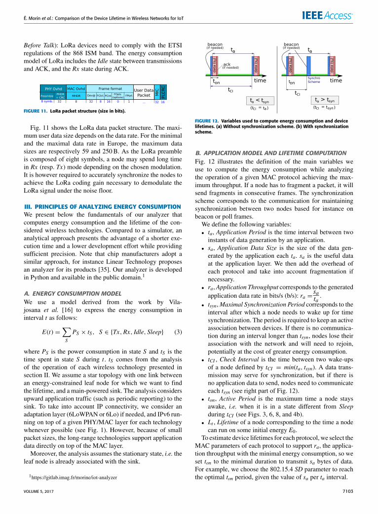
Before Talk): LoRa devices need to comply with the ETSIregulations of the 868 ISM band. The energy consumptionmodel of LoRa includes the Idle state between transmissionsand ACK, and the Rx state during ACK.

FIGURE 11. LoRa packet structure (size in bits).

Fig. 11 shows the LoRa data packet structure. The maxi-mum user data size depends on the data rate. For the minimaland the maximal data rate in Europe, the maximum datasizes are respectively 59 and 250B. As the LoRa preambleis composed of eight symbols, a node may spend long timein Rx (resp. Tx) mode depending on the chosen modulation.It is however required to accurately synchronize the nodes toachieve the LoRa coding gain necessary to demodulate theLoRa signal under the noise floor.

III. PRINCIPLES OF ANALYZING ENERGY CONSUMPTIONWe present below the fundamentals of our analyzer thatcomputes energy consumption and the lifetime of the con-sidered wireless technologies. Compared to a simulator, ananalytical approach presents the advantage of a shorter exe-cution time and a lower development effort while providingsufficient precision. Note that chip manufacturers adopt asimilar approach, for instance Linear Technology proposesan analyzer for its products [35]. Our analyzer is developedin Python and available in the public domain.1

A. ENERGY CONSUMPTION MODELWe use a model derived from the work by Vila-josana et al. [16] to express the energy consumption ininterval t as follows:

E(t) =∑S

PS × tS , S ∈ {Tx,Rx, Idle, Sleep} (3)

where PS is the power consumption in state S and tS is thetime spent in state S during t . tS comes from the analysisof the operation of each wireless technology presented insection II. We assume a star topology with one link betweenan energy-constrained leaf node for which we want to findthe lifetime, and a main-powered sink. The analysis considersupward application traffic (such as periodic reporting) to thesink. To take into account IP connectivity, we consider anadaptation layer (6LoWPAN or 6Lo) if needed, and IPv6 run-ning on top of a given PHY/MAC layer for each technologywhenever possible (see Fig. 1). However, because of smallpacket sizes, the long-range technologies support applicationdata directly on top of the MAC layer.

Moreover, the analysis assumes the stationary state, i.e. theleaf node is already associated with the sink.

1https://gitlab.imag.fr/morine/iot-analyzer

FIGURE 12. Variables used to compute energy consumption and devicelifetimes. (a) Without synchronization scheme. (b) With synchronizationscheme.

B. APPLICATION MODEL AND LIFETIME COMPUTATIONFig. 12 illustrates the definition of the main variables weuse to compute the energy consumption while analyzingthe operation of a given MAC protocol achieving the max-imum throughput. If a node has to fragment a packet, it willsend fragments in consecutive frames. The synchronizationscheme corresponds to the communication for maintainingsynchronization between two nodes based for instance onbeacon or poll frames.

We define the following variables:• ta, Application Period is the time interval between twoinstants of data generation by an application.

• sa, Application Data Size is the size of the data gen-erated by the application each ta. sa is the useful dataat the application layer. We then add the overhead ofeach protocol and take into account fragmentation ifnecessary.

• ra,Application Throughput corresponds to the generatedapplication data rate in bits/s (b/s): ra =

sata.

• tsyn,Maximal Synchronization Period corresponds to theinterval after which a node needs to wake up for timesynchronization. The period is required to keep an activeassociation between devices. If there is no communica-tion during an interval longer than tsyn, nodes lose theirassociation with the network and will need to rejoin,potentially at the cost of greater energy consumption.

• tCI , Check Interval is the time between two wake-upsof a node defined by tCI = min(ta, tsyn). A data trans-mission may serve for synchronization, but if there isno application data to send, nodes need to communicateeach tsyn (see right part of Fig. 12).

• ton, Active Period is the maximum time a node staysawake, i.e. when it is in a state different from Sleepduring tCI (see Figs. 3, 6, 8, and 4b).

• Lt , Lifetime of a node corresponding to the time a nodecan run on some initial energy E0.

To estimate device lifetimes for each protocol, we select theMAC parameters of each protocol to support ra, the applica-tion throughput with the minimal energy consumption, so weset ton to the minimal duration to transmit sa bytes of data.For example, we choose the 802.15.4 SD parameter to reachthe optimal ton period, given the value of sa per ta interval.

VOLUME 5, 2017 7103


If a technology cannot support given application through-put ra, it does not appear on the curves. The representation ofa technology stops when the application traffic correspondsto the maximal capacity of the given protocol.

FIGURE 13. Lifetime computation algorithm.

Based on the variables and the operation principles of eachMAC layer (explained in Section III-A), we compute theenergy consumption over one ta with Eq. 3, in which PS ,the power consumption in state S, is multiplied by tS , thetime spent in state S during one ta. Our lifetime algorithm(see Fig. 13) computes the energy consumed per ta as afunction of application throughput ra and derives Lt , thelifetime of a node. Lt is the number of ta a node can run untilthe initial energy E0 is exhausted.

C. PACKET LOSS MODELFor technologies that use retransmissions, we take intoaccount lost data packets due to imperfect transmission con-ditions or collisions in the following way. Let pfer and prerbe the packet error rate in the forward, respectively reverse,direction: a data packet sent from a node will be lost withprobability pfer while its acknowledgment will suffer from theloss probability of prer . The probability of a lost transmissionat the MAC layer is thus:

PER = pfer + (1− pfer )× prer . (4)

If prer is small compared to pfer (small ACK packets), theprobability reduces to PER = pfer . Assuming packet loss

probability PER, a node performs the following number oftransmissions on the average:

Ntr =1

1− PER. (5)

In the comparisons, we will choose a given level of PER andcompute the energy consumption required to send Ntr dataframes followed by an ACK for one packet generated by theapplication layer.

FIGURE 14. Algorithm of the ComputeEnergyToSendData function.

Fig. 14 gives the details of theComputeEnergyToSendDatafunction in which we take into account the energy con-sumption due to data retransmissions within each applicationperiod ta.

D. BATTERY MODELWe assume an initial battery energy of E0 = 13.5 kJ corre-sponding to two AAA batteries (1250mAh under 1.5V each)and a simple battery model with leakage Eleak of 5% per year,as well as a cutoff voltage when the residual energy reaches10% of E0. For fair comparisons, we assume the same batteryfor all technologies even though a smaller battery can be usedfor some protocols.

IV. IMPACT OF HARDWARE PLATFORMS ANDCHOICE OF THEIR PARAMETERSTo compare the technologies on the same fair basis, we needto choose the hardware parameters for the power consump-tion values. The idea is to identify the parameters that resultin the smallest energy consumption for each technology.

A. TECHNOLOGY-DEPENDENT PARAMETERSWe start with the main parameters of the standards, presentedin Table 3. We also assume 802.15.4 CCADuration of 128µsand use the default TSCH interval values (see TSCH-MACPIB attributes [8]):• timeslotLength = 10ms,• tsTxOffset = 2.120ms,• and tsRxAckDelay = 800µs.

7104 VOLUME 5, 2017


FIGURE 15. Impact of hardware platforms on the lifetime, E0 = 13.5 kJ. (a) Varying sa, constant ta = 100 s. (b) Varying sa, constant ta = 1 s. The legendapplies to both (a) and (b).

TABLE 3. Technology parameters.

TABLE 4. Hardware platform parameters.

B. HARDWARE PLATFORM PARAMETERSWe consider several hardware platforms summarized inTable 4 and evaluate the impact of their power consumptionparameters of Table 2 on the lifetime. By a hardware platformwe mean a SoC with a microcontroller and a radio module.

Fig. 15 compares the lifetimes for the initial energyE0 = 13.5 kJ, constant ta, and varying sa from 1B to 10 kB.This figure clearly shows an important impact of the hardwareparameters: for instance, the lifetime of 802.11 PSM variesfrom ∼ 1.5 to ∼ 4 years for different 802.11 PSM platforms,when ta = 1 s (see Fig. 15b) and ra = 10B/s. The effectis even more important for ta = 100 s (see Fig. 15a).Large differences for 802.15.4 and BLE platforms are alsonotable.

2assuming GreenNet STM32 CPU.

We can notice that the lifetimes are not ranked by thevalues of PTx and PRx , e.g. most of the 802.11 PSM plat-forms perform better than 802.15.4 TelosB even though theTelosB Tx and Rx power consumption is lower than that of802.11 PSM. Actually, the power consumption in these statesis a decisive factor for high data rates (small ta), but when thedata rate is lower (e.g. ta = 100 s), the Tx and Rx powerconsumption becomes less important. In this case, contraryto the common belief, the technologies are ranked by theirPsleep power, since nodes spend much more time in the sleepstate. Hence, hardware designers should also concentrate onthis value in addition to minimizing the Tx and Rx powerconsumption.

TABLE 5. Hardware parameters used for comparisons.

For a fair comparison, we have examined a range of hard-ware platform solutions and used the best-in-class param-eter value for each technology (denoted by the SelectedMin-energy in Tables 4, 5, and Fig. 15). In doing so, we haveeffectively modeled a composite platform that offers ideal-ized performance and results in the best trade-off betweentheir Pidle, PTx , and PRx parameters. Here our assumptionis that while such an idealized device may not yet be onthe market, it is feasible that a single platform offering suchbest-in-class performance exists. Tables 5 and 6 summarizethe chosen hardware parameters that we use to generate theremaining results of the paper.

Moreover, we have chosen to use the same parameters forBLE, 802.15.4, and TSCH because their hardware designis similar (same transmission power and modulation com-

VOLUME 5, 2017 7105


plexity). Hence, we adopt the lowest value of GreenNetfor PIdle, the SmartMeshIP values of PRx and PIdle, alongwith the lowest Psleep value of BLE112. Choosing a com-mon platform presents the advantage of a fair comparisonof the protocols instead of comparing hardware platforms.However, we cannot extend this approach to everytechnology—we keep a large difference in Rx and Tx powerconsumption between the 802.11 standard and the othertechnologies. The difference in the output power (0 dBmcompared to 14 and 18 dBm) is necessary to reach 802.11ranges and therefore justifies a higher Tx power consump-tion. Different modulation schemes explain the difference inthe Rx power consumption—demodulating a more complexscheme costs more energy to achieve an acceptable Bit ErrorRate (BER).

TABLE 6. SIGFOX and LoRa parameters.

For long-range technologies, we adopt the parametersin Table 6.

C. VALIDATION OF THE ANALYZERTo validate our analyzer, we have compared its results withthe SmartMeshIP power estimator [35] of TSCH provided byLinear Technology, using the lowest power mode. We haveconfigured a star topology with one node sending 10 bytes toits parent at each application period ta = 100 s (called report-ing interval) with 100% path stability. The estimator assumesa keep-alive period of tsyn ∼ 4.083 s (∼ 25 keep-alive framesduring 100 s), but it does not exploit the possibility of timesynchronization during data exchange. In this setup, the totalaverage mote current estimated for a downlink slotframe of1024 slots is 4.3µA for a voltage of 3.6V. In a comparablesetup, our analyzer gives the average current consumptionof 4.317µA, less than 1% error.

We have also compared the average energy consumptionof 802.15.4 with the measured value on the GreenNet plat-form [18]: the average current consumption was 3µA forBO = 4 (Beacon Interval of 240ms) with the possibility toskip beacons by the leaf node with a maximum time of tsyn,SO = 1 (Superframe Duration of 15.36ms), and application

3Based on TD1202 [46] with GreenNet microcontroller and BLE112power in sleep state.

4Based on SX1272 [47] with GreenNet microcontroller and BLE112power in sleep state.

period ta = 4min. In an equivalent setup, our analyzer com-putes an average current consumption of 2.46µA. The 18%difference is mainly due to a simplification inherent in ourmodel that does not take into account the energy consumptionof state transitions, nor that of the temperature sensor used inthe GreenNet measurements.

In addition, we have compared the 100B data frame perfor-mance for BLE and 802.15.4 with the performance reportedby Siekkinen et al. [15]. We modify BLE parameters to fitBLE4.0 specification [48], to compare equivalent scenarios.Our results for BLE gives 460KB/J, while 433KB/J wasreported by Siekkinen et al. Similarly, we find 180KB/Jfor the 802.15.4 standard, while Siekkinen et al. reported168KB/J. In both cases, the difference is less than 7%.

To validate the analyzer for long range technologies,we have compared its output with the values measured byMartinez et. al [17] for transmission of a single 12-bytedata packet (i.e. the maximum size for the SIGFOX technol-ogy). In the previous section, we have assumed data packetswithout security for all technologies, but to set up a faircomparison, we have added an additional overhead of 2B tothe minimal SIFGOX packet presented in Fig. 10, becauseSIGFOX imposes the use of HMACs for message authentica-tion at theMAC layer. Martinez et al.measured a current loadof 50mA for three consecutive transmissions of ∼2 s each.Assuming a 3V voltage, this value corresponds to 900mJ.Our analyzer computes a transmission time of 6.24 s with anenergy consumption of 917.28mJ (less than a 5% difference).

Finally, we have compared our results with LoRa measure-ments [17]: for transmission of a 15B data packet and assum-ing a maximum LoRa spread factor, the measured energyconsumption is ∼213mJ. In a similar setup, we compute aconsumed energy of 224mJ, which corresponds to a differ-ence of ∼5%.

These comparisons show that our analyzer yields datawithin 5%-7% of most published measured values andbroadly confirms the consistency of our approach.

V. COMPARISONS OF DEVICE LIFETIMESHaving confirmed the validity of our analyzer, we nowpresent the predicted device lifetimes for the following threecases:

1) assess the impact of application parameters without anypacket loss or clock drift.

2) evaluate the impact of a limited packet loss probabilitywithout clock drift.

3) assess the impact of imperfect clocks with clock drift(but no packet loss).

A. IMPACT OF APPLICATION PARAMETERS,NO PACKET LOSSFig. 16 presents the comparison of the lifetime for fixedvalues of application period ta = 1 day, 100 s, 1 s, and10ms, and for varying data size sa, which results in varyingthroughput ra. As there is no packet loss, PER = 0.

7106 VOLUME 5, 2017


FIGURE 16. Different ta and data size sa in bytes, leading to varying ra, impact lifetime for a starting energy E0 = 13.5 kJ, PER = 0. The bottom x-axis isthe data size in bytes per ta while the top x-axis presents the corresponding data rate ra in b/s. No packet loss or clock drift is assumed. (a) legend.(b) varying sa, constant ta = 1 day. (c) varying sa, constant ta = 100 s. (d) varying sa, constant ta = 1 s. (e) varying sa, constant ta = 10 ms.

With the separation of application period ta and data sizesa, we can distinguish between the energy consumption ofan application that generates sa = 10B every second and anapplication sending sa = 600B every minute, even thoughfor both cases ra = 80 b/s. In the first case, there are 60 trans-missions with the corresponding protocol overhead, whereasin the second case, the application only sends the minimumnumber of frames, depending on the chosen technologymaxi-mum data packet size. This effect explains, for instance, whythe lifetime for a given ra (e.g. 80 b/s) is higher in Fig. 16cthan in Fig. 16d.

The figures include the results for TSCH (marked as6-State Model TSCH with dashed lines) based on a moresophisticated model of energy consumption with two addi-tional states available on recent 802.15.4 platforms thatcan turn their microcontroller off when transmitting [16](see Fig. 17).

For the sub-1GHz frequency band, the ETSI regula-tion recommends a certain duty cycle depending on theused sub-band (e.g. 0.1% for 863-870MHz and 1% for

FIGURE 17. 6-State energy consumption model of TSCH.

868-868.6MHz) when no Listen Before Talk and FrequencyAgility mechanisms are used. Hence, in our study, we dis-play the result for 0.1% as a solid line and the resultfor 1% as a dotted line for the concerned technologies(SIGFOX and LoRA). The duty cycle limit of 1% determinesthe maximal capacity of SIGFOX at 1 kb/s and 100 b/s. More-over, the marketing limitation of SIGFOX to 140 packets perday further limits the capacity of SIGFOX at 1 kb/s and itcorresponds to the 1% duty cycle at 100 b/s.

VOLUME 5, 2017 7107


1) VERY LOW TRAFFIC INTENSITY (ta = 1 DAY)Fig. 16b shows the lifetime comparison for very low trafficintensity ta = 1 day corresponding to the operating condi-tions of long-range technologies. We observe that BLE and802.15.4 achieve the best lifetimes. LoRa performs remark-ably well with an only slightly lower lifetime compared to theshort-range BLE and 802.15.4 standards. SIGFOX achievessimilar lifetimes to LoRa only for extremely low ra, since theavailable bit rate of SIGFOX is 11 times smaller than that ofLoRa.

SIGFOX and LoRa consume more energy as the datasize sa increases. Their lifetime drops because they can onlyhandle small data packet sizes—fragmentation often occurs,which increases the overhead, and consequently the energyconsumption. Moreover, to reach the targeted long ranges,they use high transmission power, which contributes to theincreased energy consumption when they need to transmit forlonger periods.

As seen in Fig. 16b and 16c, SIGFOXandLoRa suffer fromcapacity limitations due to the ETSI regulation in the sub-1GHz band. In addition, ETSI regulation requires that nodesdo not transmit more than a certain number of consecutiveframes per hour. Thus, SIGFOX or LoRa nodes that musttransmit for more than 3.6 s (for 0.1% duty cycle) will have todelay some packets to the next hour, which impacts latency.

A SIGFOX node requires three transmissions to send onedata frame, before it is acknowledged by the base station.In this case, the limit of messages per hour leads to anincapacity to respect the duty cycle limitation in the 863 −870MHz with the rate of 100 b/s. Hence, we advise at leastthe use of the 1% tolerable sub-band to compete with otherIoT technologies.

802.11ah performs significantly worse than LoRa for smalldata sizes and outperforms it for larger data sizes. 802.11ahalso outperforms 802.11 PSM and obtains similar perfor-mance to TSCH. Note that all 802.11ah curves are overlaidin Fig. 16b: we have used the same Psleep value for the three802.11ah technologies (see Table 5). As Psleep value is thedetermining factor for a synchronized technology for verylow data rates, we understand the overlay of the curves.

2) LOW TRAFFIC INTENSITY (ta = 100 s)For sporadic application traffic, BLE achieves the longestlifetime with the 802.15.4 performance not too far behindfor small data sizes (see Fig. 16c). For larger data sizes inFig. 16c, the US variant of 802.11ah with 16MHz of band-width becomes an interesting solution after BLE. In theseconditions, the important overhead of 802.11ah packets ismitigated by a larger maximum data size. For this reason,the fragmentation happens less often than for BLE, whichdecreases the ratio overhead/data for 802.11ah.

Contrary to the findings by Tozlu regarding 802.15.4 and802.11 PSM [2], [49], Fig. 16c shows that 802.15.4 consumesless energy in most cases of low data traffic (up to throughputof 80 b/s) and obtains much longer lifetimes. We can explain

this result with the lower energy consumption of our 802.15.4platform compared to TelosB used in the paper by Tozlu—asexplained earlier, we have chosen the most efficient platformto compute the lifetime of 802.15.4 (see Table 4). The lifetimeof 802.11 PSM becomes better than 802.15.4 only for verylong packets (greater than 1.5 kB), not a usual size for IoTapplications.

3) MEDIUM AND HIGH TRAFFIC INTENSITY (ta = 1 s, 10 ms)For medium and high intensity traffic (see Fig. 16d and 16e,note also the logarithmic y-axis), BLE obtains the longestlifetime although 802.15.4 is traditionally expected to bebetter.

We can identify mainly two reasons for this result:• The 802.15.4 PHY layer is less efficient than BLE dueto a spreading factor of 8 that reduces the bit rate of802.15.4 from 2Mb/s to 250 kb/s, whereas BLE usesthe maximum rate of 2Mb/s. Hence, the bit rate of BLEis 8 times higher than 802.15.4, which leads to a lowerenergy consumption.

• Fragmentation in 802.15.4 starts from 120B of usefulinformation, whereas BLE starts fragmenting at 245B.Since the overhead for a data frame does not depend onthe packet size, 802.15.4 is less efficient than BLE forpackets bigger than 120B.

To validate this explanation, we have changed the bitrate of 802.15.4 to 2Mb/s and set the data frame size to245B. In this setup, 802.15.4 comes close to BLE (as shownin Fig. 19).

Moreover, Figure 19 displays the variation in terms of theBLE energy efficiency performance when selecting differentmodes of Bluetooth Specification 5.0 [4]: the highest avail-able data rate leads to a lower energy consumption becauseit results in the minimal time in radio consuming modes forsimilar overhead (see BLE data packets in Fig. 5).

Our results confirm the findings by Siekkinen et al. [15].They showed that, in the stationary phase, 802.15.4 transmitsless data than BLE for the same amount of energy. Siekkinenet al. also obtained their results on a hardware platform equiv-alent to BLE and 802.15.4. BLE is thus the best technologyin terms of the energy consumption for medium and highdata rates. Nevertheless, it suffers from capacity limitationfor larger data sizes. Note that the case presented in Fig. 16ecorresponds for some technologies to always-on nodes, whenoperating at their maximum capacity (represented by the endof a curve).

For sa > 100B, 802.11 PSM outperforms 802.15.4(see Fig. 16d) and becomes the second most energy-efficienttechnology up to sa > 500B, for which US-only 802.11ah(MCS9, 16MHz) with high modulation rates and large band-width becomes the most energy-efficient technology.

We note that the performance of 802.11ah with a smallerchannel bandwidth, even with high modulation indices suchas the maximum European rate (MCS 8, 2MHz, 7.8Mb/s),is worse than or equivalent to that of 802.11 PSM due to thedifference in the data rate.

7108 VOLUME 5, 2017


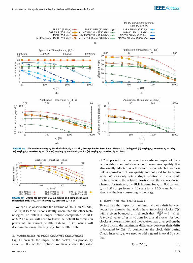
FIGURE 18. Lifetime for varying ra, No clock drift, E0 = 13.5 kJ, Average Packet Error Rate (PER) = 0.2. (a) legend. (b) varying sa, constant ta = 1 day.(c) varying sa, constant ta = 100 s. (d) varying sa, constant ta = 1 s. (e) varying sa, constant ta = 10 ms.

FIGURE 19. Liftime for different BLE 5.0 modes and comparison withtheoretical 2Mb/s 802.15.4 (varying sa, constant ta = 1 s).

We can also observe that the lifetime of 802.11ah MCS10,1MHz, 0.15Mb/s is consistently worse than the other tech-nologies. To obtain a longer lifetime comparable to BLEor 802.15.4, we will need to lower the default transmissionpower of this variant of 802.11ah to 0 dBm, which willdecrease the range, the key objective of 802.11ah.

B. ROBUSTNESS TO POOR CHANNEL CONDITIONSFig. 18 presents the impact of the packet loss probabilityPER = 0.2 on the lifetime. We have chosen the value

of 20% packet loss to represent a significant impact of chan-nel conditions and interference on transmission quality. It isalso usually adopted as a threshold below which a wirelesslink is considered of low quality and not used for transmis-sions. We can only note a slight variation in the absolutelifetime values: the relative positions of the curves do notchange. For instance, the BLE lifetime for ra = 800 b/s withta = 100 s drops from ∼ 15 years to ∼ 13.5 years, but stillstands as the less consuming technology.

C. IMPACT OF THE CLOCK DRIFTTo evaluate the impact of handling the clock drift betweennodes, we assume that nodes have imperfect clocks C(t)with a given bounded drift 1 such that | dC(t)dt − 1| ≤ 1.A typical value of 1 is 40 ppm for crystal clocks. As bothclocks at the transmitter and the receivermay diverge from theperfect clock, the maximum difference between their driftsis bounded by 21. To compensate the clock drift duringCheck Interval tCI , we need to add a guard interval Tg suchthat:

Tg = 21tCI . (6)

VOLUME 5, 2017 7109


TABLE 7. Lifetimes of representative applications, 40 ppm Clock drift, PER = 0.2, and maximum European available rates.

For instance, if tCI = 100 s and 1 = 40 ppm, the guardinterval is 8ms.

FIGURE 20. Timing relationships.

Fig. 20 presents timing relationships between a transmitterand a receiver that need to be awake for a data transmission.The first case assumes perfect clocks so Tx and Rx happenat the same time, which is the baseline case we used togenerate Fig. 16. Three other cases illustrate the operationwith a guard interval Tg tolerating a maximal relative driftof 21 (see Eq. 6) and the situation with different values ofrelative drift (−21, 0, and +21). Note that the case of −21corresponds, from the energy consumption point of view, tothe same situation as the case without the guard interval.Hence, Fig. 16 also gives us the values for −21.To show the impact of the guard interval and the clock drift

on the energy consumption, we have chosen to generate theresults of Fig. 16 for the drift of +21 (with 1 = 40 ppm)for which the receiving node needs to stay awake duringthe longest interval: Fig. 21 shows the corresponding results.We can see that for all synchronous technologies, the timewasted during the guard interval Tg in Rx state leads to con-siderable shorter lifetimes, more than 20% shorter for ta =1 day and BLE (approximately 23.5 years compared to 30).

Note also that for higher traffic intensity, the influence ofthese factors is smaller, so Fig. 21c is almost the same asFig. 16d. In this case, small ta mitigates the wasted time ofTg, since Tg is proportional to tCI that depends on ta.

The impact of the clock drift on the TSCH lifetimeis smaller than for other technologies: less than 10% forta = 1 daywith the enhanced statemodel since TSCH already

specifies a default guard interval of 1ms to compensate for animperfect clock.

For ultra low traffic intensity, LoRa and SIGFOX achievethe best lifetimes, the same ones as previously, thanks totheir asynchronous operation: they do not need to wake upin advance to compensate for the clock drift.

These results call for an adaptive synchronization scheme.Instead of consuming too much energy in guard time andsynchronization maintenance, it may be beneficial for a nodeto lose association, and then reconnect when needed for adata exchange. For example, to maximize efficiency over thelong term, a BLE node would disconnect from the networkduring sleep mode, then reconnect during wake-up. There isan additional overhead for reconnection, but it may be smallerthan the overhead due to clock synchronization. Nevertheless,we note that some mechanisms of clock drift compensationalready exist to cope with the drift issue [50].

D. LIFETIMES OF REPRESENTATIVE APPLICATIONSOur study aims at helping engineers and IoT applicationdevelopers to select the best technology depending on givenapplication requirements. Table 7 summarizes the lifetimesone can expect in a given representative application assumingthe optimal operating conditions of an IoT device with twoAAA batteries. The analyzer computes the lifetimes for thecorresponding application data rates (sa/ta) presented in thefirst column of Table 7.

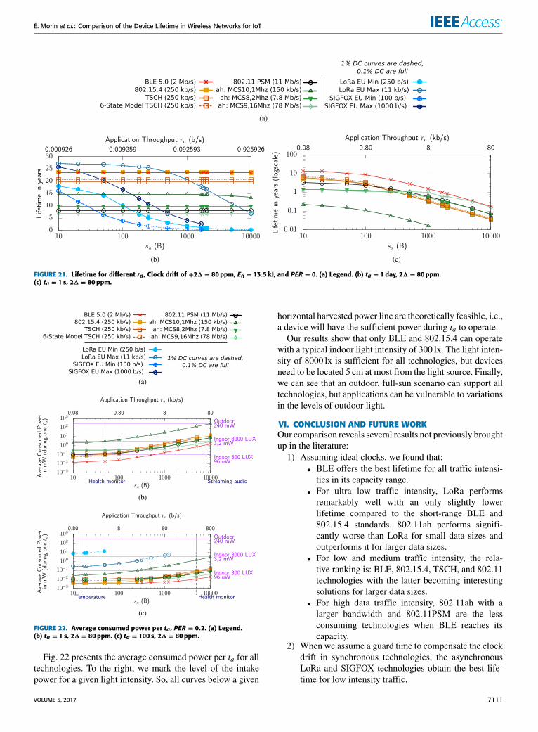
E. ENERGY HARVESTING IoT DEVICESIn this section, we address the issue of IoT devices thatharvest energy from the environment and store energy in asmall capacity battery (e.g. 20mAh). Such devices do nothave a fixed initial amount of energy that determines theirlifetime, but instead, they harvest energy intermittently andthen consume it when operating.

TABLE 8. Harvested power.

We take the example of a GreenNet node with a solar panelof '18 cm2 [18] with the indoor and outdoor values of theharvested power presented in Table 8.

7110 VOLUME 5, 2017


FIGURE 21. Lifetime for different ra, Clock drift of +21 = 80 ppm, E0 = 13.5 kJ, and PER = 0. (a) Legend. (b) ta = 1 day, 21 = 80 ppm.(c) ta = 1 s, 21 = 80 ppm.

FIGURE 22. Average consumed power per ta, PER = 0.2. (a) Legend.(b) ta = 1 s, 21 = 80 ppm. (c) ta = 100 s, 21 = 80 ppm.

Fig. 22 presents the average consumed power per ta for alltechnologies. To the right, we mark the level of the intakepower for a given light intensity. So, all curves below a given

horizontal harvested power line are theoretically feasible, i.e.,a device will have the sufficient power during ta to operate.Our results show that only BLE and 802.15.4 can operate

with a typical indoor light intensity of 300 lx. The light inten-sity of 8000 lx is sufficient for all technologies, but devicesneed to be located 5 cm at most from the light source. Finally,we can see that an outdoor, full-sun scenario can support alltechnologies, but applications can be vulnerable to variationsin the levels of outdoor light.

VI. CONCLUSION AND FUTURE WORKOur comparison reveals several results not previously broughtup in the literature:

1) Assuming ideal clocks, we found that:• BLE offers the best lifetime for all traffic intensi-ties in its capacity range.

• For ultra low traffic intensity, LoRa performsremarkably well with an only slightly lowerlifetime compared to the short-range BLE and802.15.4 standards. 802.11ah performs signifi-cantly worse than LoRa for small data sizes andoutperforms it for larger data sizes.

• For low and medium traffic intensity, the rela-tive ranking is: BLE, 802.15.4, TSCH, and 802.11technologies with the latter becoming interestingsolutions for larger data sizes.

• For high data traffic intensity, 802.11ah with alarger bandwidth and 802.11PSM are the lessconsuming technologies when BLE reaches itscapacity.

2) When we assume a guard time to compensate the clockdrift in synchronous technologies, the asynchronousLoRa and SIGFOX technologies obtain the best life-time for low intensity traffic.

VOLUME 5, 2017 7111


3) Contrary to the common belief that power consumptionin Sleep state is negligible, Psleep becomes a deter-mining factor of the device lifetime for low trafficintensities while the consumption in Tx and Rx statesstill remains important for higher traffic intensity.

4) Taking into account the energy spent in data frameretransmissions due to corrupted frames and colli-sions does not change the relative ranking of thetechnologies.

5) The current long-range technologies operating in thesub-1GHz frequency band with important duty cyclelimitations, which reduces their capacity, are not readyto support energy harvesting yet.

We have also shown that 802.15.4 consumes less energythan 802.11 PSM for low intensity traffic, which restrains thefindings by Tozlu [2]: the lifetime of 802.11 PSM is onlybetter than 802.15.4 for higher traffic intensity and longerpackets.

With respect to the existing literature, our paper providesa unique contribution in several aspects. First, our papergoes beyond several existing comparisons of IoT technolo-gies and PHY/MAC layers for sensor networks [9]–[13]that described the features of different solutions and theirlimitations without proposing a comparison on an equalbasis. Some papers limited their analysis to two technolo-gies: 802.15.4 vs. 802.11ah [14] and BLE vs. 802.15.4 [15]by using different energy consumption metrics: energy totransmit a packet (mJ/packet) vs. energy utility (kB/J), whichmakes transitive comparisons difficult.

Second, with respect to energy consumption models, muchresearch focused on physical layer aspects without takinginto account MAC operation [19]–[23]. Polastre et al. [25]initiated a realistic model of Mica2 under B-MAC furtherenhanced with the precise representations of energy con-sumption for 802.15.4 [17], [18], TSCH [16], [17], andSIGFOX [17]. We have extended this approach to deal withall the considered technologies.

Moreover, we can also note that the models of the physicallayer operation [19]–[23] neglected the impact of the micro-controller on energy consumption. This assumption is oftenjustified by the low value of microcontroller power consump-tion compared to the radio. However, even if the value islow, the accumulated energy consumption over long periodsmakes it significant. Our results show that the value of Psleep,the microcontroller power consumption in sleep mode, canbe a determining factor depending on the application traffic,so Psleep must be taken into account in a precise analysis ofenergy consumption.

Finally, our analyzer represents another progress beyondthe current state of the art. It implements the energy con-sumption model for all technologies and takes into accountseveral aspects missing in the previous studies: the over-all overhead of IP connectivity, clock drift compensationmechanisms, and packet losses. It provides a means forquick estimation of the lifetime based on the most importantparameters.

The main goal of the analysis was to evaluate energyconsumption for a given available throughput while tak-ing into account the most important parameters and factors.Nevertheless, other aspects may impact the choice of a giventechnology such as the range, total network capacity, spectralefficiency, scalability, and latency. In the future, the energyconsumption analysis can be extended along the followingresearch directions:

• Compare long range technologies with multi-hop net-works that may cover the same distances. The goalis to take the approach adopted by Lampin [52] tocompare star networks with those supporting multi-hopoperation.

• Enhance the energy consumption model with additionalstates and non-instantaneous transitions.

• Integrate other long range technologies such as802.15.4g [53], RPMA (Random Phase MultipleAccess) by Ingenu [54], or NarrowBand IoT [55].

• Optimize all aspects of energy consumption and perfor-mance for a given application scenario under constraints,for instance a given limited frequency band.

Beyond the analysis presented in this paper, the com-parison has also raised our interest in interoperability andmixing different technologies. We have shown that the costof keeping an active connection, i.e. the synchronization cost,is sometimes too high. Hence, an interesting research issueis to improve the device lifetime by proposing an adaptivescheme for time synchronization: BLE can transmit data inadvertising packets, so it may be beneficial to disconnectfrom a master and operate in non-connected mode for sparsetraffic applications. This approach can also lower energyconsumption in other technologies.

Another issue is to explore how the key features of theconsidered technologies can cooperate in the IoT context tofit the needs of different application traffic requirements suchas monitoring and delay-sensitive traffic, while obtaining suf-ficiently long lifetimes. We plan to work on interoperabilitybetween synchronous technologies such as 802.15.4e andasynchronous ones such as BLE in data-advertising mode ornon beacon-enabled 802.15.4.

REFERENCES

[1] Standard for Local andMetropolitan Area Networks—Part 15.4: Low-RateWireless Personal Area Networks (LR-WPANs), IEEE Standard 802.15.4-2003, 2003.

[2] S. Tozlu, ‘‘Feasibility of Wi-Fi enabled sensors for Internet of Things,’’in Proc. 7th Int. Wireless Commun. Mobile Comput. Conf. (IWCMC),Jul. 2011, pp. 291–296.

[3] Wireless LAN Medium Access Control (MAC) and Physical Layer (PHY)Specifications, IEEE Standard 802.11, 1999.

[4] Bluetooth SIG. [Online]. Available: https://www.bluetooth.com/specifications/adopted-specifications

[5] Draft Standard for Information Technologies Telecommunications andInformation Exchange Between Systems Local and Metropolitan AreaNetworks Specific Requirements—Part 11: Wireless LAN MediumAccess Control (MAC) and Physical Layer (PHY) Specifications—Amendment 6: Sub 1 GHz License, IEEE Standard P802.11ah/D10.0,Sep. 2016.

7112 VOLUME 5, 2017


[6] LoRa Alliance, accessed on Jan. 10, 2017. [Online]. Available: http://lora-alliance.org/

[7] SIGFOX, accessed on Jan. 10, 2017. [Online]. Available:http://www.sigfox.com/en/

[8] IEEE Standard for Local and Metropolitan Area Networks—Part 15.4:Low-Rate Wireless Personal Area Networks (LR-WPANs)—Amendment1: MAC sublayer, IEEE Standard 802.15.4e-2012 (Amendment to IEEEStandard 802.15.4-2011), 2012.

[9] A. Al-Fuqaha, M. Guizani, M. Mohammadi, M. Aledhari, and M. Ayyash,‘‘Internet of Things: A survey on enabling technologies, protocols, andapplications,’’ IEEECommun. Surveys Tuts., vol. 17, no. 4, pp. 2347–2376,4th Quart., 2015.

[10] T. Kim, I. H. Kim, Y. Sun, and Z. Jin, ‘‘Physical layer and medium accesscontrol design in energy efficient sensor networks: An overview,’’ IEEETrans. Ind. Informat., vol. 11, no. 1, pp. 2–15, Feb. 2015.

[11] A. Bachir, M. Dohler, T. Watteyne, and K. K. Leung, ‘‘MAC essentials forwireless sensor networks,’’ IEEE Commun. Surveys Tuts., vol. 12, no. 2,pp. 222–248, 2nd Quart., 2010.

[12] C. Goursaud and J.-M. Gorce, ‘‘Dedicated networks for IoT : PHY/MACstate of the art and challenges,’’ EAI Endorsed Trans. Internet Things,Oct. 2015.

[13] Q. Wang and J. Jiang, ‘‘Comparative examination on architecture andprotocol of industrial wireless sensor network standards,’’ IEEE Commun.Surveys Tuts., vol. 18, no. 3, pp. 2197–2219, 3rd Quart., 2016.

[14] B. B. Olyaei, J. Pirskanen, O. Raeesi, A. Hazmi, and M. Valkama, ‘‘Per-formance comparison between slotted IEEE 802.15.4 and IEEE 802.1 lahin IoT based applications,’’ in Proc. 9th IEEE Int. Conf. Wireless MobileComput., Netw. Commun. (WiMob), Oct. 2013, pp. 332–337.

[15] M. Siekkinen, M. Hiienkari, J. K. Nurminen, and J. Nieminen, ‘‘Howlow energy is Bluetooth low energy? Comparative measurements withZigBee/802.15.4,’’ in Proc. WCNCW, Apr. 2012, pp. 232–237.

[16] X. Vilajosana, Q. Wang, F. Chraim, T. Watteyne, T. Chang, andK. S. Pister, ‘‘A realistic energy consumption model for TSCH networks,’’IEEE Sensors J., vol. 14, no. 2, pp. 482–489, Feb. 2014.

[17] B. Martinez, M. Monton, I. Vilajosana, and J. D. Prades, ‘‘The power ofmodels: Modeling power consumption for IoT devices,’’ IEEE Sensors J.,vol. 15, no. 10, pp. 5777–5789, Oct. 2015.

[18] L.-O. Varga et al., ‘‘GreenNet: An energy-harvesting IP-enabled wirelesssensor network,’’ IEEE Internet Things J., vol. 2, no. 5, pp. 412–426,Oct. 2015.

[19] Q. Wang, M. Hempstead, and W. Yang, ‘‘A realistic power consumptionmodel for wireless sensor network devices,’’ in Proc. 3rd Annu. IEEECommun. Soc. Conf. Sensor, Mesh Ad Hoc Commun. Netw. (SECON),Reston, VA, USA, Sep. 2006, pp. 286–295.

[20] J. Li and P.Mohapatra, ‘‘Analytical modeling andmitigation techniques forthe energy hole problem in sensor networks,’’PervasiveMobile Comput. J.,vol. 3, no. 3, pp. 233–254, Jun. 2007.

[21] Q. Wang and W. Yang, ‘‘Energy consumption model for power manage-ment in wireless sensor networks,’’ in Proc. 4th Annu. IEEE Commun. Soc.Conf. Sensor, Mesh Ad Hoc Commun. Netw., Jun. 2007, pp. 142–151.

[22] H.-Y. Zhou, D.-Y. Luo, Y. Gao, and D.-C. Zuo, ‘‘Modeling of node energyconsumption for wireless sensor networks,’’Wireless Sensor Netw., vol. 3,no. 1, pp. 18–23, Jan. 2011.

[23] B. Kan, L. Cai, L. Zhao, and Y. Xu, ‘‘Energy efficient design of WSNbased on an accurate power consumption model,’’ in Proc. IEEE Int. Conf.Wireless Commun., Netw. Mobile Comput., Sep. 2007, pp. 2751–2754.

[24] J. Polastre, J. L. Hill, and D. E. Culler, ‘‘Versatile low power media accessfor wireless sensor networks,’’ in Proc. 2nd Int. Conf. Embedded Netw.Sensor Syst., Baltimore, MD, USA, Nov. 2004, pp. 95–107.

[25] J. Rahme, N. Fourty, K. A. Agha, and A. van den Bossche, ‘‘A recursivebattery model for nodes lifetime estimation in wireless sensor networks,’’in Proc. IEEE WCNC, Sydney, NSW, Australia, Apr. 2010, pp. 1–6.

[26] (2015). Introducing Thread: A New Wireless Networking Protocolfor the Home, accessed on Jan. 10, 2017. [Online]. Available:http://threadgroup.org/2014_07_Press_Release.aspx

[27] OpenThread, an Open-Source Implementation of the Thread Net-working Protocol, accessed on Jan. 10, 2017. [Online]. Available:https://github.com/openthread/openthread

[28] M. R. Palattella, N. Accettura, M. Dohler, L. A. Grieco, and G. Boggia,‘‘Traffic aware scheduling algorithm for reliable low-power multi-hopIEEE 802.15.4e networks,’’ in Proc. IEEE 23rd Int. Symp. Pers. IndoorMobile Radio Commun. (PIMRC), Sep. 2012, pp. 327–332.

[29] A. Morell, X. Vilajosana, J. L. Vicario, and T. Watteyne, ‘‘Label switchingover IEEE802.15.4e networks,’’ Trans. Emerg. Telecommun. Technol.,vol. 24, no. 5, pp. 458–475, Aug. 2013.

[30] N. Accettura, M. R. Palattella, G. Boggia, L. A. Grieco, and M. Dohler,‘‘DeTAS: A decentralized traffic aware scheduling technique enabling IoT-compliant multi-hop low-power and lossy networks,’’ in Proc. IEEE 2ndWoWMoM Workshop Internet Things, Smart Objects Services (IoT-SoS),vol. 6. Jun. 2013, pp. 1–6.

[31] 6lo Status Pages, accessed on Jan. 10, 2017. [Online]. Available:https://tools.ietf.org/wg/6lo/

[32] Wireless LAN Medium Access Control (MAC) and Physical Layer (PHY)Specifications—Amendment 4: Enhancements for Very High Throughputfor Operation in Bands below 6 GHz, IEEE Standard 802.11, 2014.

[33] E. Khorov, A. Lyakhov, A. Krotov, and A. Guschin, ‘‘A Survey on IEEE802.11ah: An Enabling Networking Technology for Smart Cities,’’ Com-put. Commun., vol. 58, pp. 53–69, Mar. 2015.

[34] O. Raeesi, J. Pirskanen, A. Hazmi, J. Talvitie, and M. Valkama, ‘‘Per-formance enhancement and evaluation of IEEE 802.11ah multi-accesspoint network using restricted access window mechanism,’’ in Proc.IEEE Int. Conf. Distrib. Comput. Sensor Syst. (DCOSS), May 2014,pp. 287–293.

[35] Linear. Dust Networks SmartMesh Power and PerformanceEstimator, accessed on Jan. 10, 2017. [Online]. Available:http://www.linear.com/docs/42452

[36] RTX. RTX4100 Datasheet DS1, accessed on Jan. 10, 2017.[Online]. Available: http://tinyurl.com/ooekop6

[37] Maxim Integrated.MAX2830 2.4GHz to 2.5GHz 802.11g/b RF Transceiverwith PA and Rx/Tx/Diversity Switch, accessed on Jan. 10, 2017.[Online]. Available: http://tinyurl.com/q3xyynj

[38] STMicroelectronics. SPWF01SA Datasheet, accessed on Oct. 16, 2015.[Online]. Available: http://tinyurl.com/or94b9l

[39] Nordic Semiconductor. nRF51822 Product Specification v3.1,accessed on Jan. 10, 2017. [Online]. Available: http://tinyurl.com/npuckqy

[40] BlueGiga. BLE112 Datasheet, accessed on Jan. 10, 2017.[Online]. Available: http://tinyurl.com/o8p8spj

[41] STMicroelectronics. BlueNRG Datasheet, accessed on Jan. 10, 2017.[Online]. Available: http://tinyurl.com/pyl5ms3

[42] P. Urard et al., ‘‘A self-powered IPv6 bidirectional wireless sensor & actu-ator network for indoor conditions,’’ in Proc. IEEE Symp. VLSI Circuits,Jun. 2015, pp. C100–C101.

[43] T. Watteyne, L. Doherty, J. Simon, and K. Pister, ‘‘Technical overview ofsmartmesh IP,’’ inProc. 7th IEEE Int. Conf. Innov.Mobile Internet ServicesUbiquitous Comput. (IMIS), Jul. 2013, pp. 547–551.

[44] Linear. SmartMeshIP Datasheet, accessed on Jan. 10, 2017. [Online].Available: http://tinyurl.com/gqyeu5v

[45] J. Polastre, R. Szewczyk, and D. Culler, ‘‘Telos: Enabling ultra-lowpower wireless research,’’ in Proc. 4th IEEE Int. Symp. Inf. Pro-cess Sensors Netw. (IPSN), 2005, pp. 364–369. [Online]. Available:http://tinyurl.com/hh6g6al

[46] Telecom-Design. TD1202 Datasheet, accessed on Jan. 10, 2017. [Online].Available: http://tinyurl.com/oclnxyo

[47] Semtech. SX1272 LoRa Datasheet, accessed on Jan. 10, 2017. [Online].Available: http://tinyurl.com/qbbzn3d

[48] Specification of Bluetooth Core v4.2, Dec. 2014.[49] S. Tozlu, M. Senel, W. Mao, and A. Keshavarzian, ‘‘Wi-Fi enabled sensors

for Internet of Things: A practical approach,’’ IEEE Commun. Mag.,vol. 50, no. 6, pp. 134–143, Jun. 2012.

[50] M. Brzozowski, H. Salomon, and P. Langendoerfer, ‘‘On efficient clockdrift prediction means and their applicability to IEEE 802.15.4,’’ inProc. IEEE/IFIP 8th Int. Conf. Embedded Ubiquitous Comput. (EUC),Dec. 2010, pp. 216–223.

[51] V. Raghunathan, A. Kansal, J. Hsu, J. Friedman, and M. Srivastava,‘‘Design considerations for solar energy harvesting wireless embeddedsystems,’’ in Proc. IEEE 4th Int. Symp. Inf. Process. Sensors Netw.,Apr. 2005, p. 64.

[52] Q. Lampin, ‘‘Urban wireless sensor networks: Applications, characteri-zation, and protocols,’’ (in French), Ph.D. dissertation, INSA De Lyon,Villeurbanne, France, 2014.

[53] K.-H. Chang and B. Mason, ‘‘The IEEE 802.15.4g standard for smartmetering utility networks,’’ in Proc. IEEE 3rd Int. Conf. Smart GridCommun. (SmartGridComm), Nov. 2012, pp. 476–480.

VOLUME 5, 2017 7113


[54] Ingenu Website, accessed on Jan. 10, 2017. [Online]. Available:https://www.ingenu.com

[55] ‘‘3GPP low power wide area technologies,’’ GSMA (GSMAssociation), White Paper, 2016. [Online]. Available:http://www.gsma.com/connectedliving/wp-content/uploads/2016/10/3GPP-Low-Power-Wide-Area-Technologies-GSMA-White-Paper.pdf

ÉLODIE MORIN is currently pursuing thePh.D. degree with Grenoble Alps University,France. She is also a Research Engineer withSTMicroelectronics and CEA-LETI, specializingin interoperability for low layers of the Internet ofThings.

She received the Engineering Diploma degree intelecommunications from INSA de Lyon in 2014.

Her research interests include low power Inter-net of Things, and routing and wireless sensor

networks.

MICKAEL MAMAN received the Engineeringdegree in electronics, telecommunications andinformatics from the Ecole Superieur de ChimiePhysique Electronique, Lyon, France, in 2006, andthe M.Sc. degree in the field of telecommuni-cations from the Institut National des SciencesAppliquées, Lyon. He has been a Research Engi-neer with CEA-LETI, the Laboratory of Elec-tronic and Information Technologies of the FrenchAtomic Energy and Alternative Energy Commis-

sion, since 2006. His research activity is concerned with MAC and networkprotocols for Internet of Things, wireless ad hoc, and sensor and body areanetworks.

ROBERTO GUIZZETTI received the degree incomputer science from the University of Milano,Italy, in 1988. He has been with STMicroelectron-ics since 1988, in various design centers of thecompany in Italy, France, and Canada. He wasinvolved in the field of digital designs and archi-tectures for various application domains, audio,video, telecommunication, with particular empha-sis on low power.

His main interests in the last few years havebeen in the Internet of Thing area, particularly in hardware and firmwarefor networks of autonomous wireless sensors and actuators.

ANDRZEJ DUDA received the Ph.D. degree fromthe Université de Paris-Sud in 1984 and the Habil-itation Diploma degree from Grenoble Univer-sity in 1994. He was an Assistant Professor withthe Université de Paris-Sud from 1983 to 1986,a Chargé de Recherche with CNRS from 1986to 1995, and a Visiting Scientist with the MITLaboratory for Computer Science from 1992 to1994. From 2002 to 2003, he was an Invited Pro-fessor with the Swiss Federal Institute of Tech-

nology, Lausanne. He is currently a Professor with the Grenoble Instituteof Technology–École Nationale Supérieure d’Informatique et de Mathéma-tiques Appliquées de Grenoble. He is also a Head of the Networks andMultimedia Group, Grenoble Informatics Laboratory. He has authored over150 papers in the areas of performance evaluation, distributed systems,multimedia, and networks.

7114 VOLUME 5, 2017

comparison of the device lifetime in wireless networks for

Documents