Comparison of Solar Occultation Flux Measurements to the 2006 TCEQ Emission Inventory and Airborne Measurements for the TexAQS II

Johan Mellqvist1, John Johansson1, Jerker Samuelsson1, Claudia Rivera1, Barry Lefer2 and Sergio Alvarez3. 1Radio and Space Science, Chalmers University of Technology, Göteborg, Sweden 2 Department of Geosciences, University of Houston, TX

3 Baylor University, Waco, TX

November 7, 2008

2

Title page: SOF measurement (foreground) of alkenes at Freeport on September 27 2006, parallel to airborne measurements by the Baylor Piper Aztec airplane.

3

Executive summary A new emission inventory has been compared to measurements of industrial leakages of VOCs, NO2 and SO2 in the vicinity of the Houston Ship Channel during the TexAQS 2006 summer campaign. The new emission inventory has been developed by the Texas Commission on Environmental Quality (TCEQ) and it is based on monitoring at 141 industrial sites during August and September of 2006. The inventory has a high time resolution of one hour and one of the aims in this study was to investigate whether observed temporal variations could be explained qualitatively by the hourly emission inventory. The hourly emission inventory lacks many emission sources and therefore an additional emission inventory, denoted “2006 Daily Inventory”, has been constructed by the TCEQ, in which the hourly inventory data has been averaged on a daily basis and then merged with emission data, for those sources not in the hourly inventory, from a yearly database. Another aim in this study was to compare the observations and the daily emission inventory quantitatively. The measurements were conducted by the Solar Occultation Flux (SOF) method and mobile DOAS, in a previous project. The estimated measurement uncertainty is 35% but to investigate this further the 2006 SOF data has been compared to emission values estimated from the NOAA WP-3D aircraft and the Baylor Piper Aztec airplane. Furthermore, the airborne data has been used to analyze the vertical mixing of the gas plumes, of relevance for the estimation of the SOF measurement uncertainty. In the study it was found that the 2006 TCEQ daily emission inventory is underestimating the emissions compared to observations by SOF. The mean discrepancy factor for the VOCs is around 10 when comparing SOF data with the 2006 daily emission inventory and another 20-50% higher when using an older annual emission inventory from 2004. For NO2 the discrepancy factors are 0.8 and 1.2, respectively when comparing mobile DOAS emission values against the 2006 and 2004 inventories while for SO2 the factors are 2.6 and 2.8, respectively. The 2006 TCEQ hourly emission inventory data shows poor correlation with the observed emissions from individual SOF transects in various sectors in the Houston shipchannel and elsewhere, when comparing for sources located within the corresponding upwind sector. However, sectors that showed large variability, order of magnitude, in the SOF measurements also shows similar variability in the hourly inventory. Airborne measurements on the Baylor Piper Aztec show that the vertical mixing of gases downwind industrial sites is quite rapid. Even at a transport time for the plume of 250 s the gases are evenly mixed up to 500 m. Part of this transport is probably caused by vertical mixing due to convection, in the order of 0.5 to 1 m/s while the rest is due to initial plume lift inside the industries. In several cases, when measuring relatively close to the industrial sources, the strong vertical mixing was not anticipated for the SOF measurements wherefore a too low windspeed was calculated from the GPS sondes used to measure the wind. The SOF emission values were therefore low by 20-30%, according to our analysis. In most cases, however, we estimate that the uncertainty was

4

smaller. All in all, the airborne measurements show that the estimated uncertainty for the SOF emission values of 35% is quite appropriate. Measurements of ethene at Mt Belvieu by the NOAA WP-3D during September of 2006 showed an average emission of 520 kg/h with an uncertainty of 50% to be compared to the average SOF value of 443 kg/h with an uncertainty of 35%. The 2006 daily EI shows an emission value of 81 kg/h here. Measurements at Sweeny on September 27 by the Baylor Piper Aztec airplane shows, in three different manners, alkene emissions between 249 to 450 kg/h, to be compared to the SOF value of 287 kg/h for the same day. The lower airborne emission estimate of 249 kg/h corresponds to one transect measured 2000 s downwind the plume, where the ratio between the alkenes and NOx was obtained and then multiplied with the NOx inventory value. The same indirect method was applied for the average of 7 transects conducted closer to the source, at 250 s plume traveling time, then yielding 414 kg/h. The third approach, was similar to the SOF one, i.e. multiplying the concentration profile, obtained by several airborne transects, with the wind, then yielding 450 kg/h. SOF measurements at Chocolate Bayou showed that 368 kg/h of alkenes were being emitted from two industrial sites to be compared to 530 kg/h obtained from the Baylor Piper Aztec measurements using the ratio between alkenes and NOx and the 2006 daily EI value of NOx. In general the comparison between SOF measurements and airborne measurements shows an agreement within 50%. It is believed that most of this discrepancy is caused by uncertainties in the airborne estimations

5

1. Introduction.................................................................................................................. 6 2. Method ......................................................................................................................... 7

2.1 The Solar Occultation Flux method ....................................................................... 7 2.2 Mobile DOAS ........................................................................................................ 8 2.3. Flux calculation..................................................................................................... 9

3. The SOF experiment during the TexAQS 2006......................................................... 10 3.1 Vertical mixing .................................................................................................... 12 3.2 Emission inventory data....................................................................................... 16

4. Results and Discussion............................................................................................... 18 4.1 Comparisons to Hourly emission inventory......................................................... 18 4.2 Comparisons to Daily emission inventory ........................................................... 23 4.3 Comparison to airborne measurements................................................................ 25

4.3.1 NOAA WP-3D.............................................................................................. 26 4.3.2 Baylor Piper Aztec ........................................................................................ 28

5. Acknowledgements .................................................................................................... 31 6. References .................................................................................................................. 32 Appendix I. Detailed comparisons between 2006 Daily EI and SOF........................... 33

A 1.1 Ethene:.............................................................................................................. 33 A1.2 Propene.............................................................................................................. 36 A 1.3 Alkanes:............................................................................................................ 38 A 1.4 SO2 ................................................................................................................... 44

Appendix II. Detailed comparisons between 2006 Hourly EI and SOF....................... 46

6

1. Introduction The SOF method is a relatively new remote sensing method based on measuring infrared intensity of solar spectra from a mobile platform (boat, automobile). From the infrared solar spectra, utilizing known absorption features and with a good knowledge of wind profile, the total mass of ethylene, propylene, alkanes and several other species along the path of the solar light can be retrieved. The SOF methodology was used in Texas during the TexAQS II Intensive Period [Mellqvist, 2007]1. The measurements, especially those of the highly reactive VOCs ethylene and propylene, suggested that these emissions were drastically underreported in the TCEQ annual emission inventory (EI). Unfortunately the EI used for comparison was not the newest one; it used 2004 data with VOCs speciated using 1999 profiles. In this project the 2006 SOF data has been compared to a newer emission inventory. The measured data has been compared against two inventories, one hourly database which is based on monitoring at 140 industrial sites during part of the 2006 field campaign and another in which the hourly data has been recalculated to a daily average and merged into the newest annual EI. The latter includes considerably more emission sources and is more realistic in terms of the magnitude of the emissions, while the former includes higher time variability, obtained through process monitoring. The SOF data has also been compared to emission values estimated from the NOAA WP-3D aircraft and the Baylor Aztec airplane, measuring in parallel with the SOF. Furthermore the airborne data has been used to analyze the vertical mixing of the gas plumes. This is of relevance for the estimation of the measurement uncertainty for the SOF measurements.

1 Available at http://www.tercairquality.org/AQR/Projects/H053.2005

7

2. Method

2.1 The Solar Occultation Flux method The SOF method is based on the recording of solar broadband infrared (IR) absorption spectra (1.8–14 µm) of IR-absorbing species. The device is mounted in a mobile vehicle with a sun tracker. The vehicle travels on roads upwind and downwind of the target sources. Measuring vertically integrated species concentrations along roads oriented crosswind and close downwind of the target source, SOF can provide the total flux of the emissions across a vertical measurement plane. This is done by integrating the data in the crosswind direction, and applying an appropriate wind-profile. This flux, after subtraction of the upwind inflow, is considered as an estimate of the emissions from the target source(s). From the measured solar spectra it is possible to retrieve a large number of species, such as aldehydes, alkanes, ammonia, CO, ethene, ethene-oxide, HF, HCl, propene, terpenes, and vinyl-chloride. The spectral retrieval is based on using multivariate analysis in which calibration spectra are fitted to the measured spectra. The calibration spectra are obtained from published reference libraries such as the HITRAN database [Benner 2003] and databases from NIST (www.NIST.gov), Pacific Northwest National Laboratories [PNL 2004] and Hanst [1996]. The spectral retrieval code used relies on principles adopted by the NDACC community (Network for the detection of atmospheric composition change), which is a global scientific community in which precise solar FTIR measurements are conducted to investigate the gas composition changes of the atmosphere. In the SOF measurements the concentration data is retrieved from the spectra using a retrieval code denoted QESOF. This code has been evaluated against several published codes developed within NDACC with agreement within 3%.

8

Figure 1. In the Solar Occultation Flux method (SOF) gases are measured by observing solar light in the infrared portion of the solar spectrum. The instrument is placed in a vehicle which is moved across the plume. From the accumulated mass measured across the plume the flux of gas is obtained by multiplication with the windspeed. (Illustration Karin Sjöberg).

2.2 Mobile DOAS In addition to the SOF system, a UV/visible system was used to measure gas fluxes of NO2 and SO2. This system measures scattered light in the zenith and does not utilize direct solar light in contrast to the SOF instrument. Therefore it is also possible to conduct measurements under cloudy conditions. The mobile system and spectral retrieval was originally developed for volcanic measurements [Galle, 2002] and is based on differential optical absorption spectroscopy (DOAS) [Platt 1979]. The mobile DOAS collects scattered ultraviolet light by means of a telescope coupled to a quartz fiber and the light is transferred into either of two spectrometers with a spectral resolution of 0.6 nm and spectral ranges 280-420 nm (SO2) and 336-480 nm (NO2), respectively. The column of SO2 is retrieved between 310-320 nm and NO2 between 425-435 nm using a custom code (mobile DOAS). This code has the same retrieval routines as the DOASIS package developed at University of Heidelberg by Stephan Kraus [DOASIS]. The calibration spectra for both species are obtained from Vandaele [1994] with an estimated uncertainty of a few percent. The mobile mini-DOAS instrument is mounted in a vehicle and measurements are performed traversing the plume, at different distances from the source, perpendicular to the plume direction. To calculate the gas emission, the wind direction and speed is also required, in the same manner as for the SOF technique (see section 2.3).

9

2.3. Flux calculation The gas flux in the mobile-DOAS and SOF method is obtained first by adding the column measurements conducted across the gas plume. The integrated mass of the key species across the plume is hence obtained. To obtain the flux this value is then multiplied by the average windspeed of the plume, uaverage. The flux calculation is shown in Eq. 1. Here x corresponds to the travel direction, z to the height direction, u’ to the windspeed orthogonal to the travel direction (x), Zsun to the distance to the sun, and Hmix to the maximum height of the plume. For the solar measurements the slant angle of the sun is compensated for, by multiplying the concentration with the cosine factor of the solar zenith angle.

dxxcolumnudxdzzuzconcfluxx

xaverage

x

x

Zsun

∫∫ ∫ =⎟⎟⎠

⎞⎜⎜⎝

⎛⋅⋅=

2

1

2

1 0

)(')(')( Eq. 1

Where

∫

∫ ⋅

= Hmix

o

Hmix

average

dz

dzuu

'' , ∫ ⋅=

Zsun

dzzconccolumn )(

The measurement and determination of the suitable windspeed for SOF is not straightforward to obtain as winds are usually complex close to the ground and increase with the height above a surface. What helps the situation is that SOF measurements only can be done in sunny conditions. This is advantageous since it corresponds to unstable meteorological conditions for which wind gradients are smoothed out by convection. Over relatively flat terrain the mean wind varies less than 20% between 20 and 100 m height using standard calculations of logarithmic wind. This is further supported by meteorological sonde measurements conducted during the TexAQS 2006 and modeling [Kihlman, 2005b] using the TAPM model [Hurley 2005]. In addition, for such meteorological conditions, with considerable convection, the emission plume from an industry mixes rather quickly vertically giving a more or less homogeneous distribution of the pollutant versus height through the mixing layer even 10 km downwind. In addition to the atmospheric mixing, the plumes from process industries exhibit an initial lift since they are usually hotter than the surrounding air. This rapid well-mixed assumption has been investigated further by using airborne measurements as is shown in section 2.3.

10

3. The SOF experiment during the TexAQS 2006 During the month of September 2006 SOF measurements were conducted with the aim of pinpointing and quantifying the largest industrial emission sources of VOCs and other species. About 10 days of measurements were conducted in the vicinity of the Houston ship channel area (HSC), 2 days in Texas City, 2 days in Sweeny and 1 day at Freeport and Chocolate Bayou. On a given day multiple measurements of the emission sources were conducted and the sources were enclosed in a “measurement box” by measuring both upwind (to eliminate background sources) and downwind (to capture the enclosed sources). During the project coordinated measurements with two airplanes, a Piper Aztec from the Baylor University [Alvarez, 2007] and the NOAA WP-3D [Gouw, 2008] were conducted on several occasions. The former carried VOC canisters for speciation and conventional instruments for continuous measurements of NOx and SO2. It also carried a Rapid Alkene Detector (RAD), an instrument based on the chemiluminescence technique with a sum response for several alkenes. The NOAA WP-3D carried a full suite of measurements and in particular a laser photo acoustic sensor for ethene. In Figure 2 and Figure 3 the SOF experiment is illustrated. The measurements were typically conducted at 0.5 to 3 km distance from the sources. The assumption, as discussed in the previous section, is that the plume is distributed from the ground up to several hundred meters height and that the wind varies little with height. This will be further discussed in section 3.1 below.

Figure 2. The SOF experiment during the TexAQS 2006 campaign is illustrated here.

11

Figure 3. SOF sectors in the Houston ship channel into which the emissions were divided for analysis. The sectors are named: 1. Allen Genoa Rd, 2. Davison Street, 3. Deer Park, 4. Battleground Rd, 5. Miller Cutoff Rd, 6. Sens Rd, 7. Baytown, 8. Mt. Belvieu. Also shown is the typical path or “SOF Box” traveled by the SOF vehicle (red track of existing roads) for sampling emissions from sectors 1 through 7. Sector 8 in the NE of the figure bounds the Mt. Belvieu source complex. To the south of sector 5 in the SOF Box is the Bayport source complex. Also shown are the locations of the LaPorte profiler (just south of sector 6) and the two sodars (Channelview north of sector 3 and Waterworks near the western edge of sector 2. These provided wind data in addition to periodical GPS sonde launches near Lynchburg Ferry in the northern part of sector 4 (courtesy of Noor Gillani).

To obtain the wind information Global Positioning System (GPS) sondes were launched within the project. In the analysis the average wind up to 200 m or 500 m has been used depending on the distance to the sources. In addition, we made use of wind profiler data from the La Porte airport and SODAR measurements in the eastern and northern part of the HSC. To investigate the uncertainties in the wind the various measurements during the field campaign were compared to the average wind over the first 500 m above ground, see Table 1. It can be seen that all windspeed measurements are within ±30% of each other, except for the ground stations which on average are 30% lower, as to be expected. For the wind direction all measurements are within ±15o, which corresponds to a 10% error in most cases in this study. Table 1. Comparison of wind measurements. This comparison includes measurements errors, systematic spatial wind differences, differences due to averaging time - the profiler and SODARs all correspond to 30 minute averages while the GPS sondes travel through the first 500 m layer in 90 s.

Wind measurement Relative difference from GPS sonde windspeed (0-500m)

Difference from GPS sonde wind direction (0-500m)

Laporte wind profiler (0-500 m) (-3±27)% (2±15)o GPS sonde (0-200 m) (-6±15)% (2±9)o SODAR waterworks (0-100 m) (-7±24)% (7±16)o SODAR HRM4 (0-100 m) (-12±18)% (2±18)o Ground stations (CAMS, 10 m) (-29±21)% (12±21)o

12

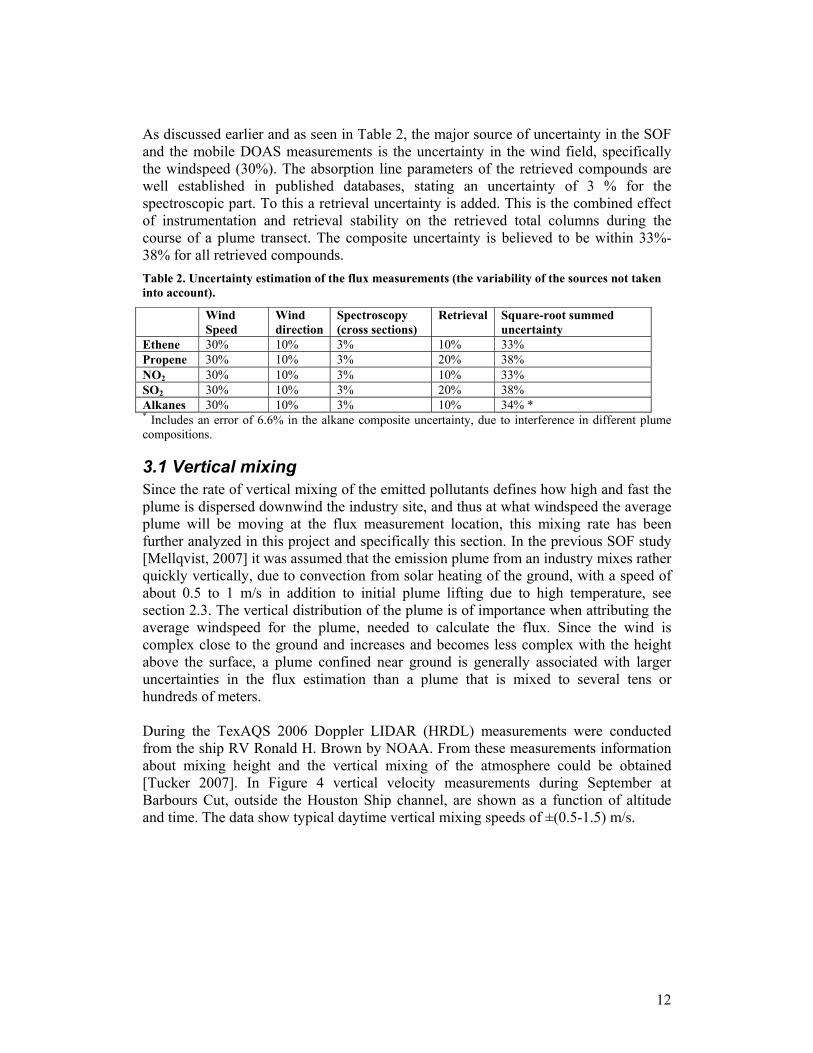
As discussed earlier and as seen in Table 2, the major source of uncertainty in the SOF and the mobile DOAS measurements is the uncertainty in the wind field, specifically the windspeed (30%). The absorption line parameters of the retrieved compounds are well established in published databases, stating an uncertainty of 3 % for the spectroscopic part. To this a retrieval uncertainty is added. This is the combined effect of instrumentation and retrieval stability on the retrieved total columns during the course of a plume transect. The composite uncertainty is believed to be within 33%-38% for all retrieved compounds. Table 2. Uncertainty estimation of the flux measurements (the variability of the sources not taken into account).

Wind Speed

Wind direction

Spectroscopy (cross sections)

Retrieval Square-root summed uncertainty

Ethene 30% 10% 3% 10% 33% Propene 30% 10% 3% 20% 38% NO2 30% 10% 3% 10% 33% SO2 30% 10% 3% 20% 38% Alkanes 30% 10% 3% 10% 34% * * Includes an error of 6.6% in the alkane composite uncertainty, due to interference in different plume compositions.

3.1 Vertical mixing Since the rate of vertical mixing of the emitted pollutants defines how high and fast the plume is dispersed downwind the industry site, and thus at what windspeed the average plume will be moving at the flux measurement location, this mixing rate has been further analyzed in this project and specifically this section. In the previous SOF study [Mellqvist, 2007] it was assumed that the emission plume from an industry mixes rather quickly vertically, due to convection from solar heating of the ground, with a speed of about 0.5 to 1 m/s in addition to initial plume lifting due to high temperature, see section 2.3. The vertical distribution of the plume is of importance when attributing the average windspeed for the plume, needed to calculate the flux. Since the wind is complex close to the ground and increases and becomes less complex with the height above the surface, a plume confined near ground is generally associated with larger uncertainties in the flux estimation than a plume that is mixed to several tens or hundreds of meters. During the TexAQS 2006 Doppler LIDAR (HRDL) measurements were conducted from the ship RV Ronald H. Brown by NOAA. From these measurements information about mixing height and the vertical mixing of the atmosphere could be obtained [Tucker 2007]. In Figure 4 vertical velocity measurements during September at Barbours Cut, outside the Houston Ship channel, are shown as a function of altitude and time. The data show typical daytime vertical mixing speeds of ±(0.5-1.5) m/s.

13

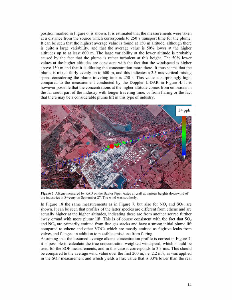
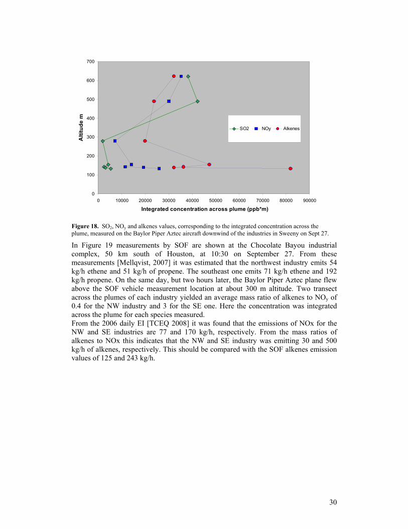
Figure 4. Vertical wind data from Doppler LIDAR measurement on the Ron Brown research vessel positioned at Barbours Cut outside the Houston Ship channel. Adapted from Tuck [2007] In Figure 5 the Sweeny industrial complex is shown which is situated 90 km SW of Houston. The picture was taken from the Baylor Aztec aircraft measuring north of the facility on September 27, 2006. The total alkene concentration in ppb is plotted versus position in Figure 6. The measurements were conducted with a RAD (Rapid alkene detector) instrument [Alvarez 2007] at various heights in the same airmass in which the SOF instrument was measuring.

Figure 5. Photo taken from The Piper Aztec aircraft downwind of Sweeny (NE part of the transect in Figure 6). Adapted from Alvarez et al. [2007]. In Figure 7 the integrated concentration values, red circles, across the plume is shown versus height. In addition the windprofile measured by the GPS sounding, from the

14

position marked in Figure 6, is shown. It is estimated that the measurements were taken at a distance from the source which corresponds to 250 s transport time for the plume. It can be seen that the highest average value is found at 150 m altitude, although there is quite a large variability, and that the average value is 50% lower at the higher altitudes up to at least 600 m. The large variability at the lower altitude is probably caused by the fact that the plume is rather turbulent at this height. The 50% lower values at the higher altitudes are consistent with the fact that the windspeed is higher above 150 m and that it is diluting the concentration more there. It thus seems that the plume is mixed fairly evenly up to 600 m, and this indicates a 2.5 m/s vertical mixing speed considering the plume traveling time is 250 s. This value is surprisingly high, compared to the measurement conducted by the Doppler LIDAR in Figure 4. It is however possible that the concentrations at the higher altitude comes from emissions in the far south part of the industry with longer traveling time, or from flaring or the fact that there may be a considerable plume lift in this type of industry.

Figure 6. Alkene measured by RAD on the Baylor Piper Aztec aircraft at various heights downwind of the industries in Sweeny on September 27. The wind was southerly.

In Figure 18 the same measurements as in Figure 7, but also for NOy and SO2, are shown. It can be seen that profiles of the latter species are different from ethene and are actually higher at the higher altitudes, indicating these are from another source further away or/and with more plume lift. This is of course consistent with the fact that SO2 and NOx are primarily emitted from flue gas stacks and have a strong initial plume lift compared to ethene and other VOCs which are mostly emitted as fugitive leaks from valves and flanges, in addition to possible emissions from flaring. Assuming that the assumed average alkene concentration profile is correct in Figure 7, it is possible to calculate the true concentration weighted windspeed, which should be used for the SOF measurements, and in this case it corresponds to 3.3 m/s. This should be compared to the average wind value over the first 200 m, i.e. 2.2 m/s, as was applied in the SOF measurement and which yields a flux value that is 33% lower than the real

34 ppb

GPS Sonde

15

one. It should be noted that the vertical wind profile at Sweeny had a stronger gradient than usually encountered, which makes the flux uncertainty larger than normal. Similar measurements to the one in Sweeny were made by the Baylor Piper Aztec airplane at Freeport on the same day. At a distance from the source corresponding to a plume traveling time of 250 s the main part of the plume was again found up to 150 m and decreasing to 50% at both 300 and 475 m altitude. The smaller concentration values were again consistent with the fact that the wind increased by a factor of 2 above 150 m. Also here the NOx and SO2 profiles were different from the alkene one and increased with height. Thus it seems, for the measurements at Sweeny and Freeport, that for VOCs the plume is mixed all the way up to 500 m, at a plume travel time of about 250 s downwind the source. It is unlikely that this strong plume raise is all due to normal vertical mixing due to convection of the air, since this would correspond to a vertical mixing speed of more than 2 m/s. It may instead, partly, be caused by initial plume lift due to the fact that air inside the industrial process is hotter than the surrounding air, and this may explain the strong vertical mixing observed.

0

100

200

300

400

500

600

700

0 10000 20000 30000 40000 50000 60000 70000 80000 90000

Alkenes integrated across plume (ppb*m)/(wind speed m/s*10000)

Alti

tude

m

Alkenes

Average Alkene

Wind gps sonde

Figure 7. Measurement of alkenes with the Baylor Piper Aztec, same data as in Figure 6. The integrated concentration values across the plume are shown with red circles. In addition the windprofile measured by the GPS sounding and the average alkene profile is shown.

The Baylor Piper Aztec plane also measured in Texas City on September 20, in parallel to the SOF measurements. Alkene measurements with RAD, the windprofile and the average alkene concentration profile are shown in Figure 8. The windspeed used by SOF was the average value over the first 200 m, corresponding to 3.8 m/s. This should be compared to the concentration weighted wind of 4.7 m/s. In this case the SOF measurements underestimate by 20%. We are uncertain about the plume traveling time here.

16

0

100

200

300

400

500

600

700

800

0 50000 100000 150000 200000 250000 300000

Alkene integrated across plume (ppb*m)/ (wind*10000 m/s)

Alti

tude

m

AlkeneAverage AlkeneWind gps sonde

Figure 8. Measurement of alkenes with the Baylor Piper Aztec at Texas City September 20. The integrated concentration values across the plume are shown with red circles. In addition the windprofile measured by the GPS sounding and the average alkene profile is shown.

3.2 Emission inventory data The emissions measured with SOF and Mobile DOAS in this study have been compared to three different emission inventories. The first is an emission inventory that has been derived by NOAA [Frost 2006] for the state of Texas including emissions of NOx, SO2, CO, total and selected speciated VOCs, PM2.5, and PM10 from 1858 fixed-location pollution sources statewide. The data are based on TCEQ's 2004 annual totals. The 2004 ethylene, propylene and alkane emissions for each point source have been derived from the 2004 total VOC emissions by assuming the same speciation at that point source as in 1999, the last year for which TCEQ provided complete speciation information. An extract of the database is given in appendix II. In the inventory, part of the emissions is reported as unspeciated VOC, corresponding to the total of VOC mass whose speciation was not known. In many cases much of the total VOC at a particular facility may in fact be reported as unspeciated. Likewise, some facilities will only report emissions in the alkanes and not break things down further. Also, a single facility is composed of hundreds or thousands of individual emission sources. While some of these sources might have good speciation information, others might not, so there may be a mixture of speciated and unspeciated emissions from the same facility. This inventory will be referred to as 2004 Annual Inventory. The second emission inventory contains hourly emission data for 3192 sources for the time period August 15 to September 15, 2006. During that period, 141 sites in E. Texas reported their hourly emissions of VOC, NOx, CO and SO2 from predetermined industrial sources, which were selected based on the following criteria: sources subject to HRVOC (highly reactive VOC) rules, NOx and SO2 sources equipped with CEMS

17

(continuous emission monitoring system), and emissions sources located near ambient air monitoring sites. For HRVOC, the reported emissions were based on process flow monitoring (flares, cooling towers) that was required beginning in January 2006. While each source in the 2004 Annual inventory corresponds to an entire facility and reports all kinds of emissions from these sources together, this inventory reports each source within a facility and each emitted species from such a source separately. This inventory will be referred to as 2006 Hourly Inventory. The third emission inventory contains daily emission data for 102314 sources for the time period August 15 to October 15, 2006. The data are daily averages of the data in the 2006 Hourly Inventory for the sources and time periods for which that data exist and yearly emissions from 2006 for the other sources and time periods. This inventory will be referred to as 2006 Daily Inventory. The 2004 Annual Inventory is probably less accurate than the other two since it is older and since the speciation of the VOCs is based on another dataset that is even older. It is also speciated to a lesser degree than the other two, i.e. a larger part of the VOCs are unspeciated and has less spatial and temporal resolution. However, it should be noted that even though the 2006 Daily inventory reports the emission day to day, its temporal resolution is not much better than that for the 2004 Annual Inventory since yearly emissions have been used where no hourly data exist. The 2004 Annual Inventory and the 2006 Daily Inventory are complete in the sense that they cover all known emission sources at the time while the 2006 Hourly Inventory is incomplete since it only covers 3192 of the 102314 sources in the 2006 Daily Inventory. The 2004 Annual Inventory covers the entire state of Texas while the other two inventories only cover the counties of Brazoria, Chambers, Fort Bend, Galveston, Harris, Liberty, Montgomery and Waller. However, all measurements in this study have been conducted within these counties.

18

4. Results and Discussion

4.1 Comparisons to Hourly emission inventory The aim here is to investigate whether large temporal variations seen in the SOF measurements in some regions can be qualitatively explained by the hourly EI. Quantitative comparisons of the hourly EI to the SOF measurements is not relevant since the former does not cover all known emission sources and therefore underestimates the emissions. In Table 3 the average VOC emissions and their variability in the previous SOF study [Mellqvist, 2007] are shown. It can be seen that the Battleground Rd and the Deer Park sectors had the highest variability for propene while for ethene it was the Miller Cut Off Rd and the Deer Park sectors. For this reason these sectors have been studied in more detail here. Table 3. The variability of the VOC emissions measured by SOF during September 2006 is shown for several of the areas studied.

Sector/Region Ethene Propene alkanes

1. Allen Genoa Rd 93 kg/h ± 30% Not detected 1970 kg/h ± 47%

2. Davison street 122 kg/h ± 25% 150 kg/h ± 41% 3900 kg/h ± 27%

3. Deer-Park 190 kg/h ± 59% 359 kg/h ± 91% 3038 kg/h ± 40%

4. Battleground Rd 91 kg/h ± 45% 388 kg/h ± 93% 1276 kg/h ± 21%

5. Miller Cut Off Rd 184 kg/h ± 69% 229 kg/h ± 21% 437 kg/h ± 27%

7. Baytown 72 kg/h ± 29% 300 kg/h ± 29% 1176 kg/h ± 19%

8. Mt. Belvieu 443 kg/h ± 28% 488 kg/h ± 39% 874 kg/h *

Texas City 83 kg/h ± 11% 51 kg/h ± 61% 2799 kg/h ± 7%

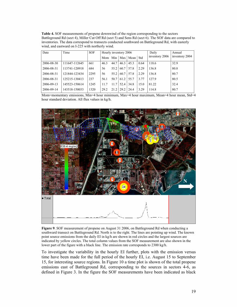
* Single measurement. In Figure 9 a SOF measurement of propene is shown on August 31 when conducting a southward transect on Battleground Rd with easterly wind. The emission sources in the 2006 daily EI are indicated. The emissions values from the SOF measurement were quite high in this transect, but decreased in later measurements. This can be seen in Table 4 were these measurements, and others, are compared to the 2006 Hourly EI. The inventory data has been obtained by adding the reported emissions from all upwind sources, up to a distance of about 10 km. In addition to the momentary EI values, also the minimum value, maximum value, mean value and standard deviation over 4 hours prior to the SOF measurement has been calculated for each sector studied. Even though the variability of the measured emissions is very high this can not be seen in the corresponding inventory data. Further comparisons of the hourly EI and all SOF measurements conducted during the TexAQS 2006 can be found in appendix II. In general the correlation is poor between the hourly EI and the SOF measurements.

19

Table 4. SOF measurements of propene downwind of the region corresponding to the sectors Battleground Rd (sect 4), Miller Cut Off Rd (sect 5) and Sens Rd (sect 6). The SOF data are compared to inventories. The data correspond to transects conducted southward on Battleground Rd, with easterly wind, and eastward on I-225 with northerly wind.

Hourly inventory 2006 Date Time SOF Mom Min Max Mean Std

Daily inventory 2006

Annual inventory 2004

2006-08-30 111647-112645 661 46.3 44.7 46.3 45.3 0.64 118.6 32.9 2006-08-31 113741-120918 684 56 55.2 60.7 57.8 2.29 136.8 80.8 2006-08-31 121844-123434 2295 56 55.2 60.7 57.8 2.29 136.8 80.7 2006-08-31 125215-130413 237 56.1 50.7 61.2 55.7 3.77 127.9 80.5 2006-09-13 145523-150614 1245 11.7 11.7 52.4 34.8 15.0 81.22 32.4 2006-09-14 143518-150033 1320 29.2 21.2 29.2 24.4 3.29 114.8 80.7

Mom=momentary emissions, Min=4 hour minimum, Max=4 hour maximum, Mean=4 hour mean, Std=4 hour standard deviation. All flux values in kg/h.

Figure 9. SOF measurement of propene on August 31 2006, on Battleground Rd when conducting a southward transect on Battleground Rd. North is to the right. The lines are pointing up wind. The known point source emissions from the daily EI in kg/h are shown in red circles and the largest sources are indicated by yellow circles. The total column values from the SOF measurement are also shown in the lower part of the figure with a black line. The emission rate corresponds to 2300 kg/h.

To investigate the variability in the hourly EI further, plots with the emission versus time have been made for the full period of the hourly EI, i.e. August 15 to September 15, for interesting source regions. In Figure 10 a time plot is shown of the total propene emissions east of Battleground Rd, corresponding to the sources in sectors 4-6, as defined in Figure 3. In the figure the SOF measurements have been indicated as black

N

20

dotted lines. It can be seen that there are generally large variations on small time scales over the whole month in this region, including some really high and sharp peaks. However, none of these variations overlapped with the SOF measurements, although it was very close for the ones conducted on September 13 and 14. It is interesting to observe that the period around August 31, when the largest measured variability was observed, is associated with larger baseline emissions in the EI. Hence, in the region east of Battleground Rd there are emission sources that can vary by an order of magnitude or more and possibly cause the observed variability on August 31. Even though there are 21 propene sources in this area in the hourly EI, all the large fluctuations seen in Figure 10 are dominated by emissions from four flares, marked with yellow circles in Figure 9. Noteworthy, is that the high propene flux measured by SOF in Figure 9 are located just downwind of these four flares.

Figure 10. Time plots of total propene emissions from the sources east of Battleground Rd (area 4-6) according to the several inventories. Blue arrows indicate height of peaks going off the chart. Black arrows pointing at dotted lines indicate the times of the measurements in Table 3.

21

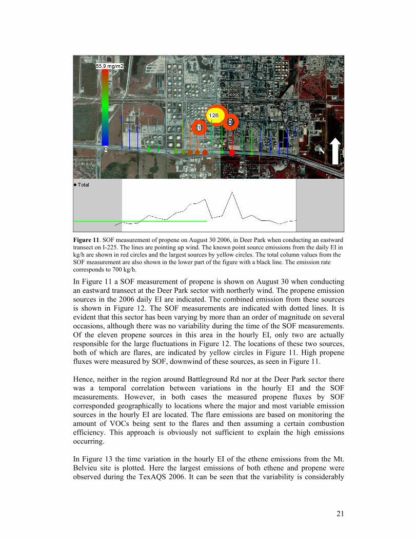
Figure 11. SOF measurement of propene on August 30 2006, in Deer Park when conducting an eastward transect on I-225. The lines are pointing up wind. The known point source emissions from the daily EI in kg/h are shown in red circles and the largest sources by yellow circles. The total column values from the SOF measurement are also shown in the lower part of the figure with a black line. The emission rate corresponds to 700 kg/h.

In Figure 11 a SOF measurement of propene is shown on August 30 when conducting an eastward transect at the Deer Park sector with northerly wind. The propene emission sources in the 2006 daily EI are indicated. The combined emission from these sources is shown in Figure 12. The SOF measurements are indicated with dotted lines. It is evident that this sector has been varying by more than an order of magnitude on several occasions, although there was no variability during the time of the SOF measurements. Of the eleven propene sources in this area in the hourly EI, only two are actually responsible for the large fluctuations in Figure 12. The locations of these two sources, both of which are flares, are indicated by yellow circles in Figure 11. High propene fluxes were measured by SOF, downwind of these sources, as seen in Figure 11. Hence, neither in the region around Battleground Rd nor at the Deer Park sector there was a temporal correlation between variations in the hourly EI and the SOF measurements. However, in both cases the measured propene fluxes by SOF corresponded geographically to locations where the major and most variable emission sources in the hourly EI are located. The flare emissions are based on monitoring the amount of VOCs being sent to the flares and then assuming a certain combustion efficiency. This approach is obviously not sufficient to explain the high emissions occurring. In Figure 13 the time variation in the hourly EI of the ethene emissions from the Mt. Belvieu site is plotted. Here the largest emissions of both ethene and propene were observed during the TexAQS 2006. It can be seen that the variability is considerably

N

22

smaller than in the time plots for Battleground and Deer Park sectors. However there were few point sources included in the Hourly EI from this area.

Figure 12. Time plots of total propene emissions from Deer Park according to inventories. Black arrows pointing at dotted lines indicate the times of SOF measurements of propene.

Figure 13. Time plots of total ethene emissions from Mt Belvieu according to inventories.

23

4.2 Comparisons to Daily emission inventory A summary of the comparisons between the daily emission inventory and the SOF and mobile DOAS measurements is shown for various Houston shipchannel sectors and other sites in Table 5 to Table 9, below. More detailed results can be found in Appendix I. For each SOF or mobile DOAS measurement, the sum of all emission sources upwind from the measurement route has been calculated, up to a distance of 10 km, both for the 2006 Daily Inventory and for the 2004 Annual Inventory. These values vary for a given region not only due to time variation in the data but also due to different routes and winds giving slightly different sets of upwind sources in the region. The complete set of such comparisons can be found in Appendix I. In Table 5 to Table 9 the averages and standard deviations of these values as well as of the SOF or mobile DOAS measurements are presented for various regions. Table 5. Average ethene emissions for measurements in September 2006. The given variability corresponds to day-to-day variations of the emissions and not uncertainty. The estimated measurement uncertainty is 30%. The sectors in the HSC were measured in northerly wind. The emission inventory is obtained from TCEQ data, see section 3.2. Sector/Region SOF 2006

(kg/h) 2006 Daily Inventory (kg/h)

2004 Annual Inventory (kg/h)

Nr. Of Meas.

1. Allen Genoa Rd 93±28 5.3±1.2 1.5±0.3 6 2. Davison Street 122±31 12.8±2.4 8.0±1.2 7 3. Deer Park 190±113 4.8±0.5 3.8±0.6 7 4. Battleground Rd WE 91±41 13.6±0.9 3.6±2.1 5 5. Miller Cutoff Rd 184±127 15.7±6.9 29.6±0.8 3 6. Sens Rd 52±0 2.8±0.0 3.3±0.0 1 7. Baytown 72±21 12.2±4.8 6.5±0.2 4 8. Mt. Belvieu 443±127 81.2±1.7 44.8±0.0 6 HSC without Mt. Belvieu 878±131 67.3±8.4 55.2±0.0 4 Bayport 163±0 22.4±0.0 6.8±0.0 1 Channelview 57±27 7.3±0.2 11.8±0.1 4 Chocolate-Bayou 136±0 42.1±0.0 10.0±0.0 1 Freeport 250±53 39.0±1.9 7.0±10.0 3 Sweeny 163±63 10.0±0.2 4.8±0.0 7 Texas City 83±9 7.6±0.0 8.6±0.0 3

*Uncertain since only one measurement, ** Direct measurement over HSC, Mt. Belvieu not included For each region we have calculated the ratio between the mean of the SOF or mobile DOAS measurements and the mean inventory emissions, both for the 2006 Daily Inventory and for the 2004 Annual Inventory. We have then calculated the geometric means (logarithmic average) and geometric standard deviations of these ratios to obtain a mean value for the discrepancy between measurements and reported emissions. For ethene the typical discrepancy factor is 9.9±80% between SOF measurements and the 2006 Daily Inventory and 17.4±110% between SOF measurements and the 2004 Annual Inventory.

24

Table 6. Average propene emissions for measurements in September 2006. The given variability corresponds to day-to-day variations of the emissions and not uncertainty. The estimated measurement uncertainty is 30%. The sectors in the HSC were measured in northerly wind. The emission inventory is obtained from TCEQ data, see section 3.2. Sector/Region SOF 2006

(kg/h) 2006 Daily Inventory (kg/h)

2004 Annual Inventory (kg/h)

Nr. of Meas.

2. Davison Street 150±62 8.9±4.3 17.1±1.4 4 3. Deer Park 359±325 13.1±2.0 8.1±0.9 6 4. Battleground Rd WE 388±360 62.6±21.2 20.3±5.9 4 5. Miller Cutoff Rd 229±47 29.8±36.5 10.7±5.0 4 6. Sens Rd 227±0 0.0±0.0 0.0±0.0 1 7. Baytown 300±86 28.8±1.6 51.3±0.0 3 8. Mt. Belvieu 488±189 37.7±0.1 12.9±0.0 3 HSC without Mt. Belvieu 1527±439 154.7±9.7 111.3±1.2 3 Bayport 203±0 13.2±0.0 10.8±0.0 1 Chocolate Bayou 273±0 29.3±0.0 24.7±0.0 1 Sweeny 127±53 7.4±0.2 5.1±0.0 3 Texas City 51±31 10.1±0.0 10.7±0.0 3

* Uncertain since only one measurement, ** Direct measurement over HSC, Mt. Belvieu not included.

For propene the typical factor is 11.2±160% between SOF measurements and the 2006 Daily Inventory and 15.4±100% between SOF measurements and the 2004 Annual Inventory. Table 7. Summary of alkane emissions as measured by SOF. Reported as averages (± 1 standard deviation, where applicable) of the daily values. The emission inventory is obtained from TCEQ data, see section 3.2.

2006 Daily Inventory (kg/h) 2004 Annual Inventory (kg/h)

Sector/Region SOF 2006 (kg/h)

A U T A U T

Nr. of Meas.

1. Allen Genoa Rd

1970±920 147±12 66±1 301±23 11±1 180±3 265±5 3

2. Davison Street 3900±878 306±21 37±3 426±26 71±3 150±4 373±10 3 3. Deer Park 3038±1204 313±123 125±34 605±201 77±2 106±11 369±43 3 4. Battleground Rd WE

1276±268 72±12 39±4 270±37 37±2 57±6 201±34 3

5. Miller Cutoff Rd

437±120 17±4 8±4 94±32 11±1 14±9 82±8 3

6. Sens Rd 494±259 15±0 6±0 44±2 11±0 6±0 38±0 2 7. Baytown 1176±218 300±35 24±2 568±63 75±0 130±0 437±1 3 8. Mt. Belvieu 874±0 126±0 64±0 334±0 150±0 111±0 263±0 1 HSC without Mt. Belvieu

12276±2851 1177±121 306±38 2288±190 291±0 633±0 1750±1 3

Sweeny 3633±963 65±0 42±0 165±0 61±0 52±0 140±0 2 Texas City 2799±201 372±7 133±0 801±17 239±0 236±1 684±0 4

Here A=Alkanes + Alcohols, U=Unspeciated VOCs, and T=Total VOCs

25

For alkanes, into which unspeciated VOCs also have been included, the typical factor is 9.9±93% between SOF measurements and the 2006 Daily Inventory and 12.4±95% between SOF measurements and the 2004 Annual Inventory. Table 8. Summary of the mobile-DOAS NO2 measurements during the TexAQS II 2006 campaign. The emission inventory is obtained from TCEQ data, see section 3.2. Sector/Region Mobile DOAS

2006 (kg/h) 2006 Daily Inventory (kg/h)

2004 Annual Inventory (kg/h)

Nr. of Meas.

Bayport 287±206 165±11 253±10 5 Baytown 443±182 633±25 867±20 19 Mt. Belvieu 313±68 189±1 269±0 6 Mt. Belvieu East 186±112 64±0 142±3 3 Channelview 340±126 155±27 371±45 3 Chocolate-Bayou 268±40 248±0 348±0 2 Freeport 754±137 904±0 1195±0 6 HSC 2315±1127 2314±35 2826±28 25 Sweeny 398±52 280±21 401±5 40 Texas City 517±177 455±9 872±9 17

For NO2 the typical factor is 1.2± 40% between mobile DOAS measurements and the 2006 Daily Inventory and 0.8±30% between mobile DOAS measurements and the 2004 Annual Inventory. Table 9. Summary of SO2 measurements during the TexAQS II 2006 campaign. The emission inventory is obtained from TCEQ data, see section 3.2. Sector/Region Mobile DOAS

2006 (kg/h) 2006 Daily Inventory

2004 Annual Inventory

Nr. of Meas.

Baytown 385±153 184±2 230±0 2 Freeport 315±135 270±0 0±0 4 Sweeny 1826±469* 166±0 241±0 24 Texas City 997±233 590±11 602±0 15

* 1 day measurement For SO2 the typical factor is 2.6±140% between mobile DOAS measurements and the 2006 Daily Inventory and 2.8±100% between mobile DOAS measurements and the 2004 Annual Inventory.

4.3 Comparison to airborne measurements Emission values obtained by the SOF method have been compared to airborne measurements conducted by the NOAA WP-3D and the Baylor Piper Aztec. There are two ways of estimating VOC emissions using airborne measurements; either in an indirect manner measuring the ratio between VOCs and NOx, assuming the NOx emissions to be well known or in a direct manner measuring the concentration across the plume at several heights and then multiplying with the windspeed, in the same manner as the SOF method is obtaining the gas fluxes.

26

The indirect method is difficult since the NOx and VOC have different sources in an industry which may results in the fact that one may have a larger plume lift than the other. This was discussed in section 3.1. This method requires that the ratio is measured in all parts of the plume. This is achievable if the measurements are conducted far away from the source, but then the mixing ratio of the species may be close to the detection limit. It also requires the NOx emissions to be well known. The direct method is uncertain since if it is conducted close to the source, it requires quite some averaging to obtain a reliable estimate, since the plume variability with height and in time is rather pronounced close to the source. If the method is applied further away, it requires an assumption about the vertical mixing of the plume, since it is difficult to make plume integrations at a lot of heights.

4.3.1 NOAA WP-3D The NOAA WP-3D carried a full suite of measurements and in particular a laser photo acoustic sensor (LPAS) measuring ethene. On September 19, the WP-3D flew a pattern around the Houston Ship Channel that was similar to that driven by the Chalmers SOF van on the same day. This is shown in Figure 6 which is taken from a recent paper by Gouw et al. [2008] and shows the column measurements by SOF compared with the results of the LPAS measurements. The aircraft ethene data was converted to column density assuming that ethene was uniformly mixed across the height of the boundary layer (BL). The BL height was estimated to be 2100±400 m using altitude profiles of potential temperature, humidity and CO measured onboard the aircraft. Figure 6 shows that both the SOF and LPAS measurements show enhancements downwind from Mt. Belvieu (plume location 1 and possibly 4) and the western and eastern parts of the Ship Channel (plume locations 2 and 3, respectively). In addition, the column measurement from the SOF and the estimates from the aircraft agreed within ~50%, suggesting that the vertical mixing of the plumes was fairly complete where the plumes were sampled by the aircraft. Gouw et al. [2007] estimates the uncertainty of the WP3-D flux measurements to 50%. In Figure 14 the emission obtained for Mt Belvieu during the TexAQS 2006 is shown for the SOF, NOAA WP-3D and the 2006 inventory. The SOF data corresponds to 6 transects (August 31, September 19 and 25) while the WP-3D data corresponds to 10 transects (September 13, 15, 19, 21, 25, 26, 27 and October 5, 6 and 13). The SOF values correspond to 443±130 kg/h, with a measurement uncertainty of 35%. For the NOAA WP-3D values the corresponding numbers are 520±140 kg/h with an uncertainty of 50%. The 2006 daily inventory corresponds to 81 kg/h.

27

Figure 15. Ethene columns derived from the NOAA WP-3D aircraft and measured by the SOF on September 19, 2009. Adapted from Gouw [2008]. The white triangles show reported emissions in TCEQ 2004 inventory.

28

0

100

200

300

400

500

600

700

SOF NOAA WP-3D Daily Inventory 2006

Ethe

ne k

g/h

Figure 16. Emissions of ethene at the Mt Belvieu industrial complex using airborne LPAS measurements from the NOAA WP-3D and the SOF method. The SOF data was measured by multiple transects on 3 days, while the airborne measurements were conducted over 10 days.

4.3.2 Baylor Piper Aztec The Baylor Piper Aztec carried a RAD instrument for measuring alkenes and several chemiluminescence instruments for measurements of NO, NO2 and NOy [Alvarez, 2007]. The RAD was calibrated for propene and is sensitive also to ethene, butadiene and isoprene. Ethene has a sensitivity which is 0.34 relative to propene and when measuring in a mixture the RAD values have to be recalibrated for that specific mixture. For example at Sweeny, only ethene and propene was detected by SOF in the plume with a molecular ratio of ethene to propene of 1.9. This ratio yields a RAD recalibration factor of 1.8. For the Chocolate Bayou facility the corresponding molecular ratio is 0.7 which yields a RAD recalibration factor of 1.4. In Figure 17 SOF measurements at the Sweeny industrial complex are shown, measured on September 27 in the afternoon. The average emission of ethene here was 160 kg/h while for propene it was 127 kg/h. Simultaneous airborne measurements by the Baylor Piper Aztec airplane was conducted, as already shown in Figure 6. Figure 18 shows the airborne data of alkenes, NOy and SO2 integrated across the plume for these measurements, about 250 s plume traveling time downwind the site. The average mass ratio of alkenes to NOy in the plume is 1.4, obtained by taking the ratio between the sum of all alkenes to the sum of all NOy. The emission rate of NOx reported for Sweeny in 2006 EI [TCEQ 2008] is 292 kg/h, and thus this implies that the emissions of alkenes correspond to 414 kg/h, obtained through multiplication with the measured alkene to NOx ratio. This should be compared with the SOF estimate of the alkene emission for this day of 287 kg/h.

29

One airborne transect was also conducted further away, about 2000 s plume traveling time downwind from Sweeny. In this case the mass ratio between alkenes and NOy was 0.82, which multiplied with the 2006 EI value for NOx of 292 kg/h yields an alkene emission rate of 240 kg/h. Emission rates of alkenes can also be calculated in another manner for the airborne data in Figure 18. In section 3.1, Figure 7, the average height concentration profile of ethene was estimated from transects at different heights. The flux from this gas profile is obtained by multiplying with the windspeed at each height and then an alkene emission value of 450 kg/h is obtained, in the same manner as in the SOF approach. Here it has been assumed that there is no ethene above 600 m altitude.

Figure 17. SOF measurement of ethene at Sweeny on September 27, 2006. The lines are pointing up wind. The known point source emissions from the 2006 daily EI in kg/h are shown in red circles. The total column values are also shown in the lower part of the figure with a black line. The average emission for three measurements on this day corresponds to 160±34 kg/h. For propene the corresponding value is 127 kg/h.

30

0

100

200

300

400

500

600

700

0 10000 20000 30000 40000 50000 60000 70000 80000 90000

Integrated concentration across plume (ppb*m)

Alti

tude

m

SO2 NOy Alkenes

Figure 18. SO2, NOy and alkenes values, corresponding to the integrated concentration across the plume, measured on the Baylor Piper Aztec aircraft downwind of the industries in Sweeny on Sept 27.

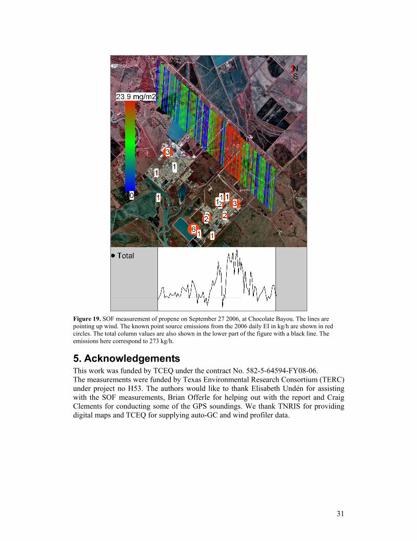
In Figure 19 measurements by SOF are shown at the Chocolate Bayou industrial complex, 50 km south of Houston, at 10:30 on September 27. From these measurements [Mellqvist, 2007] it was estimated that the northwest industry emits 54 kg/h ethene and 51 kg/h of propene. The southeast one emits 71 kg/h ethene and 192 kg/h propene. On the same day, but two hours later, the Baylor Piper Aztec plane flew above the SOF vehicle measurement location at about 300 m altitude. Two transect across the plumes of each industry yielded an average mass ratio of alkenes to NOy of 0.4 for the NW industry and 3 for the SE one. Here the concentration was integrated across the plume for each species measured. From the 2006 daily EI [TCEQ 2008] it was found that the emissions of NOx for the NW and SE industries are 77 and 170 kg/h, respectively. From the mass ratios of alkenes to NOx this indicates that the NW and SE industry was emitting 30 and 500 kg/h of alkenes, respectively. This should be compared with the SOF alkenes emission values of 125 and 243 kg/h.

31

Figure 19. SOF measurement of propene on September 27 2006, at Chocolate Bayou. The lines are pointing up wind. The known point source emissions from the 2006 daily EI in kg/h are shown in red circles. The total column values are also shown in the lower part of the figure with a black line. The emissions here correspond to 273 kg/h.

5. Acknowledgements This work was funded by TCEQ under the contract No. 582-5-64594-FY08-06. The measurements were funded by Texas Environmental Research Consortium (TERC) under project no H53. The authors would like to thank Elisabeth Undén for assisting with the SOF measurements, Brian Offerle for helping out with the report and Craig Clements for conducting some of the GPS soundings. We thank TNRIS for providing digital maps and TCEQ for supplying auto-GC and wind profiler data.

32

6. References Alvarez et al., H-63 AIRCRAFT MEASUREMENTS IN SUPPORT OF TEXAQS II, Available at http://files.harc.edu/Projects/AirQuality/Projects/H063/H063FinalReport.pdf, 2007 Benner D.C., et al., The HITRAN molecular spectroscopic database: Edition of 2000 including updates through 2001. Journal of Quantitative Spectroscopy and Radiative Transfer, 2003. 82(1-4): p. 5 DOASIS, developed by Kraus. S. Available at: http://www.iup.uni-heidelberg.de/bugtracker/projects/doasis/ Frost, G. 2006 , TEXAQS2K6, version 1, 2 August 2006, personal communication. Gouw, J., et al., Measurements of Highly Reactive VOCs Onboard the NOAA WP-3D, Principal Findings Data Analysis Workshop TexAQS II, Austin, May 29-June 01, 2007. (available at www.tceq.state.tx.us) Galle B., Oppenheimer C., Geyer A., McGonigle A. and Edmonds M., A miniaturised ultraviolet spectrometer for remote sensing of SO2 fluxes: a new tool for volcano surveillance. Journal of Volcanology, 2002. 119: p. 241-254 Gouw et al., Airborne Measurements of Ethene from Industrial Sources Using Laser Photo-Acoustic Spectroscopy, submitted to ES&T, September 2008 Hanst P.L., QASoft ´96, Database and quantitative analysis program for measurements of gases. Infrared Analysis Inc., 1996. Hurley P.J., Physick W.L., and Luhar A.K., TAPM: A practical approach to prognostic meteorological and air pollution modelling. Environmental Modelling and Software, 2005. 20(6): p. 737. Kihlman, M., Mellqvist, J. and Samuelsson, J., Monitoring of VOC emissions from three refineries in Sweden and the Oil harbour of Göteborg using the Solar Occultation Flux method, RR. report (Göteborg) No. 1, , ISSN 1653 333X, 2005a, (available at www.fluxsense.se) Mellqvist, J, Samuelsson, J., Rivera, C. Lefer, B.,, and M. Patel, Measurements of industrial emissions of VOCs, NH3, NO2 and SO2 in Texas using the Solar Occultation Flux method and mobile DOAS, Project H-53, available at http://www.tercairquality.org/AQR/Projects/H053.2005, 2007 Pacific Northwest National Laboratory. 2004 Available from: https://secure.pnl.gov/nsd/nsd.nsf/Welcome. Platt, U., Perner, D. and Pätz, H.W., "Simultaneous Measurements of Atmospheric CH2O, O3 and NO2 by Differential Optical Absorption", J. Geophys. Res., 84, 6329-6335, 1979 Tucker, S., Marine boundary Layer dynamics and heights during TexAQS 2006: HRDL measurements from the RV Brown, Principal Findings Data Analysis Workshop TexAQS II, Austin, May 29-June 01, 2007. (available at www.tceq.state.tx.us) TCEQ (2008), 2006 Point Source Emissions Inventory, Accessed October 2008 at: http://www.tceq.state.tx.us/implementation/air/industei/psei/psei.html. Vandaele, A. C.; Simon, P. C.; Guilmot, J. M.; Carleer, M.; Colin, R. Journal of Geophysical Research-Atmospheres 1994, 99, 25599-25605.

33

Appendix I. Detailed comparisons between 2006 Daily EI and SOF. Each SOF measurement has here been compared to appropriate upwind sources from inventories. All flux values in kg/h

A 1.1 Ethene: E=Ethene P=Propene O=Other alkenes U=Unspeciated VOCs Date Time Wind SOF Daily inventory 2006 Annual inventory 2004 E P O U E P O U

1. Allen Genoa Rd

2006-08-30 105705-110401 6.2 m/s, 359 ° 59.676 4.2 5.7 10 84 1.3 1.5 1.2 183 2006-08-30 132657-133424 6.0 m/s, 1 ° 105.05 3.4 4.2 7.3 50 1.3 1.1 0 159 2006-09-13 153846-154556 3.8 m/s, 6 ° 111.42 6.5 6.3 11 68 2 2.3 3.3 278 2006-09-19 102544-103202 9.4 m/s, 41 ° 131.61 6.5 5.6 10 73 1.3 1.1 1.8 178 2006-09-19 111120-111619 9.4 m/s, 41 ° 95.938 6.1 5.2 9.4 68 1.3 1.1 0.5 178 2006-09-19 143651-144139 4.5 m/s, 35 ° 51.757 5.1 2.3 5.9 63 1.3 1.5 1.7 193

Mean 92.574 5.3 4.9 9 68 1.5 1.4 1.4 195 2. Davison Street

2006-08-30 110321-110859 6.2 m/s, 359 ° 138.39 16 11 19 43 8.8 16 20 140 2006-08-30 131201-132401 6.0 m/s, 1 ° 170.57 13 7.2 14 21 8.2 16 18 32 2006-09-13 152330-152847 3.8 m/s, 6 ° 114.58 8 9.1 11 15 5.2 1.5 8.2 18 2006-09-19 101834-102430 9.4 m/s, 41 ° 66.064 13 6.9 14 17 8.1 15 18 18 2006-09-19 111702-112339 9.4 m/s, 41 ° 115.35 13 9.9 16 23 8.9 19 20 38 2006-09-19 144217-145016 4.5 m/s, 35 ° 146.73 14 13 20 39 8.9 19 20 130 2006-09-25 121422-122338 7.0 m/s, 5 ° 100.82 13 6.9 14 21 8.1 15 18 31

Mean 121.78 13 9.2 16 26 8 14 18 58 3. Deer Park

2006-08-30 111058-111530 6.2 m/s, 359 ° 401.14 4.3 14 14 91 3.3 7.5 3.3 85 2006-08-30 130148-130741 6.0 m/s, 1 ° 279.44 4.2 13 13 78 3.3 7.5 3.3 32 2006-09-13 150946-151531 3.8 m/s, 6 ° 105.39 4.1 8.8 11 66 3.3 7.5 3.3 94 2006-09-19 100637-101532 9.4 m/s, 41 ° 222.8 5.3 15 32 146 4.4 11 7.1 126 2006-09-19 112611-113153 9.4 m/s, 41 ° 67.434 5.1 14 19 85 4.4 11 6.6 124 2006-09-19 145055-145802 4.5 m/s, 35 ° 70.948 5.3 15 34 157 4.4 11 7.1 135 2006-09-25 120517-121131 7.0 m/s, 5 ° 182.74 4.9 14 27 117 3.3 7.5 3.5 39

Mean 189.98 4.8 13 21 106 3.8 9.1 4.9 91 4. Battleground Rd WE

2006-08-30 111647-111947 6.2 m/s, 359 ° 73.919 12 50 8.4 25 1.6 18 2 45 2006-09-13 150112-150614 3.8 m/s, 6 ° 157.92 15 74 4.4 33 5.5 30 2.7 45 2006-09-19 100051-100346 9.4 m/s, 41 ° 120 14 69 1.7 19 5.4 26 0.4 21

34

2006-09-19 113900-114110 9.4 m/s, 41 ° 55.894 13 63 1.7 18 4.9 9.5 0.4 19 2006-09-25 115352-115654 7.0 m/s, 5 ° 48.957 14 77 3.7 20 0.4 16 0 7.3

Mean 103.36 15 58 4 27 4.1 19 1.3 30 Battleground Rd NS

2006-08-31 105359-111214 2.3 m/s, 75 ° 158.82 47 72 39 40 14 52 26 176 2006-08-31 114943-120918 2.3 m/s, 75 ° 254.28 56 122 32 42 36 74 22 170 2006-08-31 121844-123434 2.3 m/s, 75 ° 276.42 57 126 33 43 36 74 22 173 2006-08-31 125215-131029 2.3 m/s, 75 ° 95.139 54 125 33 37 33 74 22 167 2006-09-14 143518-150033 5.6 m/s, 107 ° 479.82 70 86 16 42 36 74 22 155 2006-09-14 153654-160244 4.0 m/s, 120 ° 264.92 68 80 8 41 34 29 4 41 2006-09-14 160823-163610 4.0 m/s, 120 ° 437.32 68 80 8 41 34 29 4 41

Mean 280.96 60 99 24 41 32 58 17 132 5. Miller Cutoff Rd

2006-08-30 111935-112342 6.2 m/s, 359 ° 114.74 17 93 5.1 20 30 15 5 32 2006-09-13 145523-150126 3.8 m/s, 6 ° 362.68 23 7.1 4.8 9.8 28 2.1 2.8 14 2006-09-25 114914-115413 7.0 m/s, 5 ° 74.647 6.7 6.7 3.2 12 30 15 5 25

Mean 184.02 16 36 4.3 14 30 11 4.2 24 6. Sens Rd

2006-08-30 112342-112645 6.2 m/s, 359 ° 52.491 2.8 0 0.1 6.1 3.3 0 0 6.5

Mean 52.491 2.8 0 0.1 6.1 3.3 0 0 6.5 7. Baytown

2006-08-30 112645-113500 6.2 m/s, 359 ° 69.728 10 30 36 29 6.6 51 24 130 2006-09-07 122202-123633 2.0 m/s, 75 ° 47.337 10 30 33 22 6.6 51 24 147 2006-09-13 144844-145409 4.6 m/s, 10 ° 104.41 20 46 47 25 6.6 51 24 130 2006-09-25 111946-112613 7.0 m/s, 5 ° 67.709 7.9 23 26 13 6.1 27 20 21

Mean 72.295 12 32 35 22 6.5 45 23 107 Baytown-Mt. Belvieu

2006-09-19 152540-154237 4.5 m/s, 35 ° 244.48 10 28 34 23 6.6 51 24 130

Mean 244.48 10 28 34 23 6.6 51 24 130 8. Mt. Belvieu

2006-08-30 113203-114235 6.2 m/s, 359 ° 354.03 79 37 19 66 45 13 6.6 128 2006-08-30 121556-122843 6.0 m/s, 1 ° 275.13 79 37 21 70 45 13 6.6 129 2006-09-19 131054-133246 6.0 m/s, 32 ° 331.29 83 38 19 64 45 13 6.6 111 2006-09-25 145616-152408 6.6 m/s, 353 ° 558.76 83 38 19 64 45 13 6.6 111 2006-09-25 155455-160559 6.6 m/s, 353 ° 535.73 82 38 18 63 45 13 6.6 111 2006-09-25 164328-170104 6.6 m/s, 353 ° 605.00 83 38 19 64 45 13 6.6 111

Mean 443.32 81 38 19 65 45 13 6.6 117 HSC without Mt. Belvieu

2006-08-30 105336-113435 6.2 m/s, 359 ° 966.72 62 167 90 291 55 111 54 723 2006-08-30 122443-133757 6.0 m/s, 1 ° 904.59 62 167 90 271 55 111 54 627 2006-09-13 143954-154606 3.8 m/s, 6 ° 985.34 82 153 98 236 55 110 54 606 2006-09-25 112958-123954 7.0 m/s, 5 ° 656.52 64 150 102 324 55 112 56 612

Mean 878.29 67 159 95 281 55 111 54 642 HSC with Channelview

2006-08-30 105336-114810 6.2 m/s, 359 ° 1398.3 148 216 147 401 112 145 72 797

35

2006-08-30 121532-133757 6.0 m/s, 1 ° 1187.5 148 215 146 388 112 145 72 759 2006-09-19 91944-103750 9.4 m/s, 41 ° 1223.6 154 200 159 444 112 145 72 783 2006-09-19 110303-114734 9.4 m/s, 41 ° 834.67 154 200 157 437 112 145 72 764 2006-09-19 142646-152019 4.5 m/s, 35 ° 707.06 154 200 157 435 112 145 72 761

Mean 1070.2 152 206 153 421 112 145 72 773 Bayport

2006-09-26 105413-110917 2.3 m/s, 38 ° 163.47 22 15 4.2 45 6.8 12 2.2 42

Mean 163.47 22 15 4.2 45 6.8 12 2.2 42 Channelview

2006-08-31 164824-170305 3.0 m/s, 43 ° 46.268 7.3 11 32 32 12 20 9.9 11 2006-08-31 175645-181336 2.0 m/s, 126 ° 22.751 7.3 11 32 32 12 20 9.9 11 2006-09-19 135516-140833 6.0 m/s, 32 ° 60.682 7.6 12 35 45 12 20 10 18 2006-09-26 151530-152926 2.8 m/s, 51 ° 97.924 7 7.9 30 26 12 16 9.8 7.3

Mean 56.906 7.3 11 32 34 12 19 9.9 12 Chocolate-Bayou

2006-09-27 102700-104905 4.1 m/s, 184 ° 136.08 42 29 35 35 10 25 5 47

Mean 136.08 42 29 35 35 10 25 5 47 Freeport

2006-09-27 123732-125143 4.0 m/s, 183 ° 214.74 38 3.2 1.1 19 0 0.3 0.8 6.1 2006-09-27 130213-134434 4.0 m/s, 183 ° 325.18 42 9.2 4.6 39 21 14 1 29 2006-09-27 141652-142456 5.0 m/s, 200 ° 211.4 38 3.1 1 17 0 0.3 0.8 8.4

Mean 250.44 39 5.2 2.2 25 7 4.9 0.9 14 Sweeny

2006-09-21 114732-115435 10.0 m/s, 191 ° 54.789 10 7.6 14 41 4.8 5.1 1.9 52 2006-09-21 115539-120129 10.0 m/s, 191 ° 174.08 10 7.6 14 28 4.8 5.1 1.9 52 2006-09-21 144502-150202 10.0 m/s, 191 ° 273.31 10 7.6 14 41 4.8 5.1 1.9 52 2006-09-27 161602-162221 2.2 m/s, 185 ° 136.46 9.6 7.1 13 38 4.8 5.1 1.9 51 2006-09-27 164232-165114 2.2 m/s, 185 ° 124.65 10 7.6 14 41 4.8 5.1 1.9 52 2006-09-27 170757-171611 2.2 m/s, 185 ° 186.59 9.6 7.1 13 39 4.8 5.1 1.9 51 2006-09-27 172557-174958 2.2 m/s, 185 ° 191.87 10 7.6 14 43 4.8 5.1 1.9 52

Mean 163.11 10 7.5 14 39 4.8 5.1 1.9 52 Sweeny West

2006-09-21 132035-132445 8.0 m/s, 197 ° 226.1 5.2 4.4 9.6 15 4.8 5.1 1.9 51 2006-09-21 134231-134656 8.0 m/s, 197 ° 111.81 6.9 6.1 9.2 16 4.8 5.1 1.9 40 2006-09-21 142454-142830 8.0 m/s, 197 ° 59.74 5.2 4.4 9.6 15 4.8 5.1 1.9 51

Mean 132.55 5.8 5 9.4 15 4.8 5.1 1.9 48 Texas City

2006-09-20 92909-93843 3.8 m/s, 60 ° 80.476 7.6 10 92 132 8.6 11 3 234 2006-09-20 120822-121536 3.8 m/s, 60 ° 72.333 7.6 10 92 125 8.6 11 3 231 2006-09-20 122824-123530 3.8 m/s, 60 ° 95.196 7.6 10 92 127 8.6 11 3 231

Mean 82.668 7.6 10 92 128 8.6 11 3 232

36

A1.2 Propene: E=Ethene P=Propene O=Other alkenes U=Unspeciated VOCs Date Time Wind SOF Daily inventory 2006 Annual inventory 2004 E P O U E P O U

2. Davison Street

2006-08-30 110321-110859 6.2 m/s, 359 ° 147.6 16 11 19 43 8.8 16 20 140 2006-09-13 152847-154100 3.8 m/s, 6 ° 115.18 7.3 1.9 6.1 19 3.6 16 12 125 2006-09-19 144217-145016 4.5 m/s, 35 ° 84.818 14 13 20 38 8.9 19 20 130 2006-09-25 121318-122234 7.0 m/s, 5 ° 250.65 13 9.2 14 22 8.2 18 18 32

Mean 149.56 13 8.9 15 30 7.4 17 18 107 3. Deer Park

2006-08-30 111058-111530 6.2 m/s, 359 ° 710.17 4.3 14 14 91 3.3 7.5 3.3 85 2006-08-30 130148-130741 6.0 m/s, 1 ° 895.21 4.2 13 13 78 3.3 7.5 3.3 32 2006-09-13 150946-151531 3.8 m/s, 6 ° 245.8 4.1 8.8 11 66 3.3 7.5 3.3 94 2006-09-19 112611-113153 9.4 m/s, 41 ° 144.1 5 15 32 130 4.4 9.4 4.8 121 2006-09-19 145055-145802 4.5 m/s, 35 ° 17.407 5.3 15 34 150 4.4 9.4 5.4 130 2006-09-25 120413-121027 7.0 m/s, 5 ° 140.05 4.9 13 18 114 3.3 7.5 3.3 32

Mean 358.79 4.6 13 20 105 3.7 8.1 3.9 82 4. Battleground Rd WE

2006-08-30 111647-111947 6.2 m/s, 359 ° 144.53 8.8 26 8.4 25 1.6 18 2 46 2006-09-13 150112-150614 3.8 m/s, 6 ° 1010.3 15 74 4.4 33 5.5 30 2.7 45 2006-09-19 145735-150249 4.5 m/s, 35 ° 213.19 14 75 4 34 0.8 16 0 24 2006-09-25 115424-115654 7.0 m/s, 5 ° 185.33 14 75 3.7 19 0.4 16 0 7.3

Mean 388.33 13 63 5.1 28 2.1 20 1.2 31 Battleground Rd NS

2006-08-31 113741-120918 2.3 m/s, 75 ° 683.61 61 137 41 51 41 81 27 186 2006-08-31 121844-123434 2.3 m/s, 75 ° 2294.6 58 137 39 41 37 81 27 161 2006-08-31 125215-130413 2.3 m/s, 75 ° 237.47 54 128 33 31 37 80 24 155 2006-09-14 143518-150033 5.6 m/s, 107 ° 1319.8 79 115 47 50 38 81 27 161

Mean 1133.9 63 129 40 43 38 81 26 166 5. Miller Cutoff Rd

2006-08-30 111935-112342 6.2 m/s, 359 ° 289.2 17 93 5.1 20 30 15 5 32 2006-08-30 124648-125018 6.0 m/s, 1 ° 235.49 3 5.3 2.5 4.7 26 13 1.2 21 2006-09-13 145523-150126 3.8 m/s, 6 ° 234.48 23 7.1 4.8 9.8 28 2.1 2.8 14 2006-09-25 114821-115352 7.0 m/s, 5 ° 158.34 12 14 3.3 7.1 30 13 3.2 24

Mean 229.38 14 30 3.9 10 29 11 3 23 6. Sens Rd

2006-08-30 112342-112645 6.2 m/s, 359 ° 227.15 2.8 0 0.1 6.1 3.3 0 0 6.5

Mean 227.15 2.8 0 0.1 6.1 3.3 0 0 6.5 7. Baytown

37

2006-08-30 123153-123603 6.2 m/s, 359 ° 358.7 9.8 30 35 26 6.6 51 24 130 2006-09-07 122202-123633 2.0 m/s, 75 ° 177.39 10 30 33 24 6.6 51 24 125 2006-09-25 111935-112549 7.0 m/s, 5 ° 362.69 9.5 27 32 16 6.6 51 24 124

Mean 299.59 9.9 29 33 22 6.6 51 24 126 Baytown-Belvieu

2006-09-19 152630-153602 4.5 m/s, 35 ° 341.46 10 28 33 22 6.6 51 24 129

Mean 341.46 10 28 33 22 6.6 51 24 129 8. Mt. Belvieu

2006-09-19 131610-132801 6.0 m/s, 32 ° 222.07 78 38 11 62 41 13 2 110 2006-09-25 155434-160538 6.6 m/s, 353 ° 646.36 81 38 18 60 45 13 6.6 111 2006-09-25 164328-165947 6.6 m/s, 353 ° 596.18 82 38 18 63 45 13 6.6 111

Mean 488.21 80 38 16 62 44 13 5.1 111 HSC without Mt. Belvieu

2006-08-30 105336-113435 6.2 m/s, 359 ° 1837.5 62 167 91 299 55 112 56 732 2006-09-13 144350-154534 3.8 m/s, 6 ° 1837.5 82 153 98 241 55 112 56 614 2006-09-25 113404-122140 7.0 m/s, 5 ° 906.97 57 144 91 245 53 110 52 332

Mean 1527.3 67 155 93 261 54 111 54 559 HSC with Channelview

2006-08-30 105336-114810 6.2 m/s, 359 ° 1922.9 148 216 147 401 112 145 72 797 2006-09-19 110303-114734 9.4 m/s, 41 ° 1403.4 154 200 157 436 112 145 72 762 2006-09-19 142646-152019 4.5 m/s, 35 ° 764.27 154 200 157 437 112 145 72 763

Mean 1363.5 152 205 153 425 112 145 72 774 Bayport

2006-09-26 105413-110435 2.3 m/s, 38 ° 203.11 21 13 2.9 33 6.8 11 1.1 31

Mean 203.11 21 13 2.9 33 6.8 11 1.1 31 Chocolate-Bayou

2006-09-27 102333-103937 4.1 m/s, 184 273.03 42 29 31 32 10 25 5 47

Mean 273.03 42 29 31 32 10 25 5 47 Sweeny

2006-09-27 164232-165114 2.2 m/s, 185 ° 78.899 10 7.6 14 41 4.8 5.1 1.9 52 2006-09-27 170757-171611 2.2 m/s, 185 ° 200.09 9.6 7.1 13 39 4.8 5.1 1.9 51 2006-09-27 172557-173728 2.2 m/s, 185 ° 100.57 10 7.6 14 42 4.8 5.1 1.9 52

Mean 126.52 9.9 7.4 14 41 4.8 5.1 1.9 52 Sweeny West

2006-09-21 132035-132445 8.0 m/s, 197 ° 392.01 5.2 4.4 9.6 15 4.8 5.1 1.9 51 2006-09-21 134231-134656 8.0 m/s, 197 ° 109.72 6.9 6.1 9.2 16 4.8 5.1 1.9 40

Mean 250.86 6 5.2 9.4 16 4.8 5.1 1.9 46 Texas City

2006-09-20 92643-93333 3.8 m/s, 60 ° 12.967 6.8 10 92 127 8.6 11 3 231 2006-09-20 120822-121536 3.8 m/s, 60 ° 89.943 7.6 10 92 125 8.6 11 3 231 2006-09-20 122824-123530 3.8 m/s, 60 ° 50.428 7.6 10 92 127 8.6 11 3 231

Mean 51.112 7.3 10 92 126 8.6 11 3 231

38

A 1.3 Alkanes: A=Alkanes + Alcohols U=Unspeciated VOCs T=Total VOCs Date Time Wind SOF Daily inventory 2006 Annual inventory 2004 A U T A U T

1. Allen Genoa Rd

2006-09-13 122512-124109 4.6 m/s, 10 ° 1067.4 131.9 65.26 269.4 11.7 181.7 268.5 2006-09-19 174824-175647 4.9 m/s, 30.4 ° 3231.9 160.3 66.37 318.7 10.53 175.6 257.6 2006-09-25 131549-132118 6.1 m/s, 2 ° 1609.8 149.8 66.32 315.5 11.7 181.7 268.5

Mean 1969.7 147.4 65.98 301.2 11.31 179.7 264.8 2. Davison Street

2006-09-13 121916-122515 4.6 m/s, 10 ° 3076 288.8 33.28 395.7 68.25 145.7 360.3 2006-09-19 173810-174754 4.9 m/s, 30.4 ° 5117.1 294.7 39.53 423.6 74.9 148.4 384.6 2006-09-25 132054-132751 6.1 m/s, 2 ° 3507.1 335.9 39.07 459.6 69.49 154.4 374.1

Mean 3900.1 306.5 37.29 426.3 70.88 149.5 373 3. Deer Park

2006-09-13 121255-121911 4.6 m/s, 10 ° 3686.9 140.3 79.1 331.4 76.36 102.3 368.7 2006-09-19 173211-173841 4.9 m/s, 30.4 ° 4075.4 417.8 159.3 806.7 79.82 121.2 422 2006-09-25 132745-133633 6.1 m/s, 2 ° 1350.3 381.9 135.5 676.1 74.07 95.68 317.5

Mean 3037.5 313.4 124.6 604.7 76.75 106.4 369.4 4. Battleground Rd WE

2006-09-13 120933-121305 4.6 m/s, 10 ° 1636.1 69.02 39.22 255.7 38.63 60.02 202.7 2006-09-19 172202-173217 4.9 m/s, 30.4 ° 994.13 60.29 35.35 233.2 34.91 48.67 157.8 2006-09-25 133633-134116 6.1 m/s, 2 ° 1197 88.02 43.93 321.5 37.89 63.2 241.9

Mean 1275.7 72.44 39.5 270.2 37.14 57.3 200.8 5. Miller Cutoff Rd

2006-09-13 120620-120908 4.6 m/s, 10 ° 595.1 13.17 4.586 64.22 9.507 7.292 74.21 2006-09-19 171853-172155 4.9 m/s, 30.4 ° 410.59 23.14 7.149 139 9.521 7.85 77.33 2006-09-25 134116-134453 6.1 m/s, 2 ° 305.55 16.1 13.06 79.85 12.54 25.64 93.33

Mean 437.08 17.47 8.266 94.36 10.52 13.59 81.63 6. Sens Rd

2006-09-13 120043-120302 4.6 m/s, 10 ° 752.77 14.32 6.061 41.28 10.7 6.477 37.64 2006-09-25 134445-134858 6.1 m/s, 2 ° 234.35 14.93 6.091 46.04 10.7 6.477 37.64

Mean 493.56 14.63 6.076 43.66 10.7 6.477 37.64 7. Baytown

2006-08-31 151350-152352 3.0 m/s, 58 ° 1023.6 271.1 22.03 514.7 74.75 129.3 436.2 2006-09-13 115313-120025 4.6 m/s, 10 ° 1484.4 349 24.78 657.2 75.75 129.7 437.6 2006-09-25 134825-135743 6.1 m/s, 2 ° 1021 278.5 26.58 532.5 75.75 129.7 437.6

Mean 1176.3 299.5 24.46 568.1 75.42 129.5 437.1 8. Mt. Belvieu

2006-09-25 140544-141615 5.0 m/s, 359 ° 874.36 125.9 63.63 334.5 149.5 111.3 263.1

39

Mean 874.36 125.9 63.63 334.5 149.5 111.3 263.1 HSC without Mt. Belvieu

2006-09-13 115326-124109 4.6 m/s, 10 ° 11674 1006 252.6 2019 290.9 633.2 1750 2006-09-19 170808-180010 4.9 m/s, 30.4 ° 16029 1262 332.1 2422 290.9 633.6 1750 2006-09-25 131507-140016 6.1 m/s, 2 ° 9123.2 1262 332.4 2424 290.9 633.6 1752

Mean 12276 1177 305.7 2288 290.9 633.4 1750 Plant A

2006-09-30 131112-131623 4.5 m/s, 259 ° 167.07 18.51 8.123 75.44 15.04 15.83 108

Mean 167.07 18.51 8.123 75.44 15.04 15.83 108 Sweeny

2006-09-21 153950-155615 8.1 m/s, 188 ° 2670.4 64.89 41.52 164.9 61.27 51.75 140.1 2006-09-21 163545-164442 8.1 m/s, 188 ° 4596.4 64.89 41.52 164.9 61.27 51.75 140.1

Mean 3633.4 64.89 41.52 164.9 61.27 51.75 140.1 Texas City

2006-09-02 134924-140045 3.2 m/s, 67 ° 2482.2 383.9 132.8 771.6 239.1 236.6 683.9 2006-09-20 132634-133953 4.8 m/s, 81 ° 2998.9 367.5 133.2 810.7 239.1 236.6 683.9 2006-09-20 134710-140114 4.8 m/s, 81 ° 2942.7 367.5 133.2 810.7 239.1 236.6 683.9 2006-09-20 163108-164612 4.1 m/s, 112 ° 2772.3 368.2 133.2 811.3 239 235.1 683.8

Mean 2799 371.8 133.1 801.1 239.1 236.2 683.9 Texas City East

2006-09-20 170013-172417 3.2 m/s, 110.5 ° 989.56 144.4 37.76 230.5 62.76 72.15 209.2

Mean 989.56 144.4 37.76 230.5 62.76 72.15 209.2

40

NOx Date Time Wind SOF

NO2 Daily inventory 2006 Annual inventory 2004

NOx NOx

Bayport

2006-09-23 101207-103913 11.775 m/s, 187 ° 148.35 169.15 255.97 2006-09-23 105352-111738 9.95 m/s, 188.5 ° 165.4 169.02 255.97 2006-09-23 112533-113812 11.475 m/s, 190.25 ° 413.94 174.86 262.91 2006-09-23 114920-121744 11.8 m/s, 188.25 ° 75.137 169.02 255.97 2006-09-26 102231-112204 3.365 m/s, 65.5 ° 629.69 144.44 234.71

Mean 286.5 165.30 253.10 Baytown

2006-08-28 112020-114516 5.0 m/s, 180 ° 501.98 608.38 871.37 2006-08-28 121432-123212 5.0 m/s, 180 ° 71.285 608.07 870.65 2006-08-28 123524-125407 5.0 m/s, 180 ° 293.47 607.94 870.65 2006-08-28 125735-131738 5.0 m/s, 180 ° 381.34 607.94 870.65 2006-08-28 133423-135203 5.0 m/s, 180 ° 878.7 608.25 871.37 2006-08-28 141838-143639 5.0 m/s, 180 ° 609.98 608.25 871.37 2006-08-28 143952-145845 5.0 m/s, 180 ° 541.37 608.99 871.37 2006-08-28 150302-152130 5.0 m/s, 180 ° 205.91 608.38 871.37 2006-08-28 153650-155444 5.0 m/s, 180 ° 239.91 608.38 871.37 2006-08-31 160602-162406 4.2 m/s, 21.5 ° 578.75 641.17 871.37 2006-08-31 163406-165220 4.2 m/s, 21.5 ° 433.49 641.17 871.37 2006-08-31 165918-172027 4.2 m/s, 21.5 ° 652.29 641.17 871.37 2006-09-04 164614-173258 2.1 m/s, 87.9 ° 245.32 675.03 871.38 2006-09-07 120925-131106 1.5 m/s, 56 ° 381.56 666.81 871.37 2006-09-07 141235-143934 1.5 m/s, 56 ° 460.82 666.81 871.37 2006-09-07 163947-171436 1.5 m/s, 56 ° 625.76 666.77 871.37 2006-09-07 173106-175354 1.5 m/s, 56 ° 432.83 640.58 782.77 2006-09-07 175801-181804 1.5 m/s, 56 ° 442.48 666.77 871.37 2006-09-13 172858-180255 2.6 m/s, 333 ° 436.02 648.46 871.37

Mean 442.8 633.12 866.60 Mt. Belvieu

2006-09-25 150033-151854 4.9 m/s, 340.5 ° 218.44 189.47 268.72 2006-09-25 152905-153508 4.9 m/s, 340.5 ° 216.21 189.47 268.72 2006-09-25 155237-160956 7.3 m/s, 350° 351.49 189.47 268.72 2006-09-25 161634-162306 7.3 m/s, 350° 356.6 189.47 268.72 2006-09-25 164147-170833 7.3 m/s, 350° 375.56 189.47 268.72 2006-09-25 171115-171846 7.3 m/s, 350° 360.33 187.11 267.65

Mean 313.11 189.07 268.55 Belvieu East

2006-09-19 82632-83339 6.2 m/s, 64 ° 59.204 64.49 143.89 2006-09-19 85012-90048 6.2 m/s, 64 ° 167 64.49 137.37 2006-09-25 174012-175912 7.3 m/s, 350° 331.8 64.50 144.43

41

Mean 186 64.49 141.90 Channelview

2006-09-26 151507-153148 4.9 m/s, 10.5 ° 165.45 135.92 339.04 2006-09-29 141138-142438 4.0 m/s, 112 ° 395.06 192.20 434.64 2006-09-29 151454-152219 5.7 m/s, 107 ° 458.14 135.61 339.04

Mean 339.55 154.57 370.91 Chocolate-Bayou

2006-09-27 101135-104945 5.2 m/s, 188° 228.47 248.00 347.70 2006-09-27 104945-110654 5.2 m/s, 188° 307.67 248.00 347.70

Mean 268.07 248.00 347.70 Freeport

2006-09-16 124755-132149 6.6 m/s, 178° 713.33 904.41 1194.56 2006-09-22 123637-130517 12.9 m/s, 193.9 ° 517.86 904.49 1194.61 2006-09-22 140942-145053 11.9 m/s, 192.1 ° 739.66 904.49 1194.61 2006-09-27 115408-125511 4.0 m/s, 198 ° 718.49 904.49 1194.61 2006-09-27 125723-134745 4.0 m/s, 198 ° 916.89 904.32 1194.60 2006-09-27 134938-143413 4.0 m/s, 198 ° 919.42 904.32 1194.60

Mean 754.27 904.42 1194.60 HSC

2006-08-28 92408-101813 5.0 m/s, 180 ° 3310.4 2312.81 2827.21 2006-08-30 84447-93155 5.8 m/s, 12.5 ° 2950.7 2309.33 2824.99 2006-08-30 100249-105122 5.8 m/s, 12.5 ° 3104.9 2309.33 2824.99 2006-08-30 110545-115532 5.8 m/s, 12.5 ° 1283.5 2309.33 2824.99 2006-08-30 135053-143941 5.3 m/s, 327 ° 2467.2 2307.87 2824.41 2006-08-30 145624-155958 5.3 m/s, 327 ° 2847 2363.13 2824.39 2006-08-30 163104-172027 5.3 m/s, 327 ° 1768 2307.80 2824.41 2006-08-30 175041-184043 5.3 m/s, 327 ° 909.56 2307.80 2824.41 2006-08-31 83344-93704 0.7 m/s, 43.5 ° 1204.5 2341.11 2827.21 2006-08-31 94610-103513 0.7 m/s, 43.5 ° 995.31 2341.14 2827.21 2006-08-31 103727-112704 0.7 m/s, 43.5 ° 1269.2 2342.35 2827.21 2006-08-31 115343-124702 2.0 m/s, 60 ° 1851.8 2440.15 2919.32 2006-09-11 111403-121435 2.9 m/s, 77.3 ° 2443.6 2289.67 2827.21 2006-09-13 114022-133826 5.3 m/s, 4 ° 1256.3 2324.21 2820.11 2006-09-13 142152-164439 5.3 m/s, 4 ° 1033.6 2325.76 2820.11 2006-09-17 95756-104317 7.7 m/s, 192.8 ° 5132.7 2296.61 2828.28 2006-09-17 105706-114144 6.4 m/s, 195.6 ° 2524 2296.81 2827.31 2006-09-17 120125-124407 8.2 m/s, 196.6 ° 3042.3 2296.35 2827.31 2006-09-18 160638-165219 3.9 m/s, 329.8 ° 3122.7 2239.89 2723.17 2006-09-18 172056-180827 4.8 m/s, 335.3 ° 2447.8 2294.47 2825.43 2006-09-19 100505-110114 6.2 m/s, 64 ° 1374.4 2285.33 2833.74 2006-09-19 112822-121616 11.4 m/s, 49 ° 4513.1 2297.82 2828.70 2006-09-19 122212-131134 8.4 m/s, 41.5 ° 719.18 2337.00 2844.18 2006-09-19 151234-160031 5.6 m/s, 28.5 ° 3441.7 2294.79 2819.21 2006-09-19 160448-165154 5.6 m/s, 28.5 ° 2852.7 2288.77 2819.21

Mean 2314.7 2314.39 2825.79 HSC East

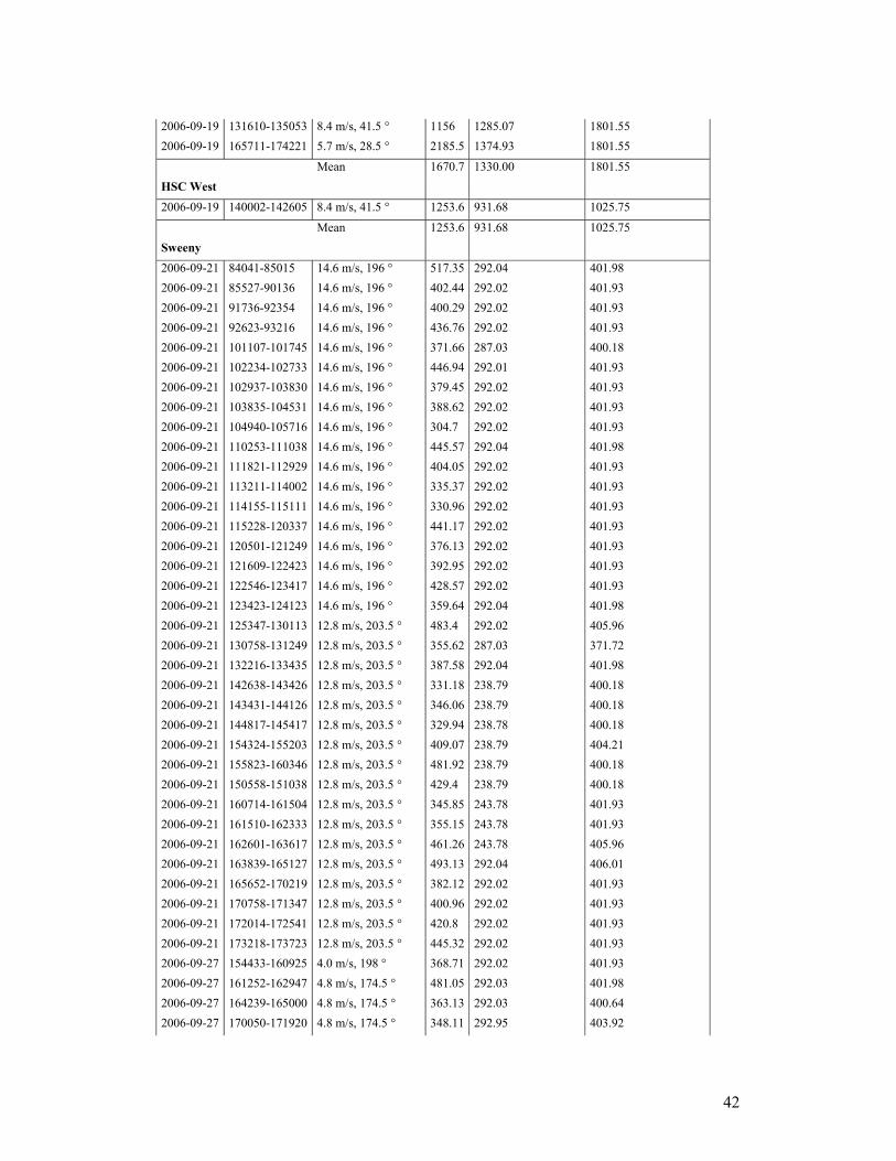
42

2006-09-19 131610-135053 8.4 m/s, 41.5 ° 1156 1285.07 1801.55 2006-09-19 165711-174221 5.7 m/s, 28.5 ° 2185.5 1374.93 1801.55

Mean 1670.7 1330.00 1801.55 HSC West

2006-09-19 140002-142605 8.4 m/s, 41.5 ° 1253.6 931.68 1025.75

Mean 1253.6 931.68 1025.75 Sweeny

2006-09-21 84041-85015 14.6 m/s, 196 ° 517.35 292.04 401.98 2006-09-21 85527-90136 14.6 m/s, 196 ° 402.44 292.02 401.93 2006-09-21 91736-92354 14.6 m/s, 196 ° 400.29 292.02 401.93 2006-09-21 92623-93216 14.6 m/s, 196 ° 436.76 292.02 401.93 2006-09-21 101107-101745 14.6 m/s, 196 ° 371.66 287.03 400.18 2006-09-21 102234-102733 14.6 m/s, 196 ° 446.94 292.01 401.93 2006-09-21 102937-103830 14.6 m/s, 196 ° 379.45 292.02 401.93 2006-09-21 103835-104531 14.6 m/s, 196 ° 388.62 292.02 401.93 2006-09-21 104940-105716 14.6 m/s, 196 ° 304.7 292.02 401.93 2006-09-21 110253-111038 14.6 m/s, 196 ° 445.57 292.04 401.98 2006-09-21 111821-112929 14.6 m/s, 196 ° 404.05 292.02 401.93 2006-09-21 113211-114002 14.6 m/s, 196 ° 335.37 292.02 401.93 2006-09-21 114155-115111 14.6 m/s, 196 ° 330.96 292.02 401.93 2006-09-21 115228-120337 14.6 m/s, 196 ° 441.17 292.02 401.93 2006-09-21 120501-121249 14.6 m/s, 196 ° 376.13 292.02 401.93 2006-09-21 121609-122423 14.6 m/s, 196 ° 392.95 292.02 401.93 2006-09-21 122546-123417 14.6 m/s, 196 ° 428.57 292.02 401.93 2006-09-21 123423-124123 14.6 m/s, 196 ° 359.64 292.04 401.98 2006-09-21 125347-130113 12.8 m/s, 203.5 ° 483.4 292.02 405.96 2006-09-21 130758-131249 12.8 m/s, 203.5 ° 355.62 287.03 371.72 2006-09-21 132216-133435 12.8 m/s, 203.5 ° 387.58 292.04 401.98 2006-09-21 142638-143426 12.8 m/s, 203.5 ° 331.18 238.79 400.18 2006-09-21 143431-144126 12.8 m/s, 203.5 ° 346.06 238.79 400.18 2006-09-21 144817-145417 12.8 m/s, 203.5 ° 329.94 238.78 400.18 2006-09-21 154324-155203 12.8 m/s, 203.5 ° 409.07 238.79 404.21 2006-09-21 155823-160346 12.8 m/s, 203.5 ° 481.92 238.79 400.18 2006-09-21 150558-151038 12.8 m/s, 203.5 ° 429.4 238.79 400.18 2006-09-21 160714-161504 12.8 m/s, 203.5 ° 345.85 243.78 401.93 2006-09-21 161510-162333 12.8 m/s, 203.5 ° 355.15 243.78 401.93 2006-09-21 162601-163617 12.8 m/s, 203.5 ° 461.26 243.78 405.96 2006-09-21 163839-165127 12.8 m/s, 203.5 ° 493.13 292.04 406.01 2006-09-21 165652-170219 12.8 m/s, 203.5 ° 382.12 292.02 401.93 2006-09-21 170758-171347 12.8 m/s, 203.5 ° 400.96 292.02 401.93 2006-09-21 172014-172541 12.8 m/s, 203.5 ° 420.8 292.02 401.93 2006-09-21 173218-173723 12.8 m/s, 203.5 ° 445.32 292.02 401.93 2006-09-27 154433-160925 4.0 m/s, 198 ° 368.71 292.02 401.93 2006-09-27 161252-162947 4.8 m/s, 174.5 ° 481.05 292.03 401.98 2006-09-27 164239-165000 4.8 m/s, 174.5 ° 363.13 292.03 400.64 2006-09-27 170050-171920 4.8 m/s, 174.5 ° 348.11 292.95 403.92

43

2006-09-27 172611-173732 4.8 m/s, 174.5 ° 343.82 292.04 401.98

Mean 398.16 280.19 401.30 Sweeny East

2006-09-03 101045-103531 5.5 m/s, 47.5 ° 96.763 60.80 0.00 2006-09-03 113837-114755 5.5 m/s, 47.5 ° 90.494 60.80 0.00 2006-09-03 115414-121825 5.5 m/s, 47.5 ° 123.29 60.80 0.00 2006-09-03 123301-125823 5.5 m/s, 47.5 ° 143.61 60.80 0.00

Mean 113.54 60.80 0.00 Texas City

2006-09-02 134540-140029 1.6 m/s, 102.4 ° 191.55 480.28 875.41 2006-09-02 140828-142302 2.2 m/s, 108 ° 202.64 478.54 866.22 2006-09-14 93000-93807 4.0 m/s, 117 ° 458.64 449.40 872.13 2006-09-14 95925-101059 4.0 m/s, 117 ° 417.9 449.42 872.13 2006-09-14 105351-110842 4.0 m/s, 117 ° 346.53 449.40 872.13 2006-09-14 113107-114706 4.0 m/s, 117 ° 373.5 449.40 872.13 2006-09-20 90240-90803 6.3 m/s, 67.5 ° 712.54 452.32 903.92 2006-09-20 101954-102741 6.3 m/s, 67.5 ° 553.1 452.28 865.55 2006-09-20 111134-111928 6.3 m/s, 67.5 ° 536.58 452.28 865.55 2006-09-20 120503-121220 6.3 m/s, 67.5 ° 535.11 452.26 865.55 2006-09-20 132412-133059 6.3 m/s, 67.5 ° 697.35 452.28 865.55 2006-09-20 140151-141334 5.7 m/s, 75 ° 420.97 453.22 866.22 2006-09-20 144052-145336 4.3 m/s, 98.5 ° 659.07 453.21 872.81 2006-09-20 152944-154006 4.3 m/s, 98.5 ° 778.84 452.26 872.13 2006-09-20 160611-161215 4.3 m/s, 98.5 ° 448.1 452.26 872.13 2006-09-20 162306-163052 4.3 m/s, 98.5 ° 724.12 453.18 872.81 2006-09-20 163803-164704 4.3 m/s, 98.5 ° 733.9 453.18 872.81

Mean 517.08 455.01 872.07 Texas City West

2006-09-02 101415-104757 3.5 m/s, 33.1 ° 930.06 348.49 627.14 2006-09-02 110122-113847 3.2 m/s, 33.7 ° 312.71 326.68 520.24 2006-09-02 123536-132201 3.8 m/s, 89.6 ° 310.89 328.76 520.24 2006-09-20 114646-121331 6.3 m/s, 67.5 ° 404.59 313.69 546.48 2006-09-20 124421-130430 6.3 m/s, 67.5 ° 499.4 312.15 520.24 2006-09-20 131452-133747 6.3 m/s, 67.5 ° 581.76 313.69 546.48 2006-09-20 134648-142054 5.7 m/s, 75 ° 393.56 313.70 546.48 2006-09-20 142525-150024 4.3 m/s, 98.5 ° 515.22 313.69 546.48 2006-09-20 150650-154145 4.3 m/s, 98.5 ° 707.29 313.69 546.48

Mean 517.28 320.50 546.69

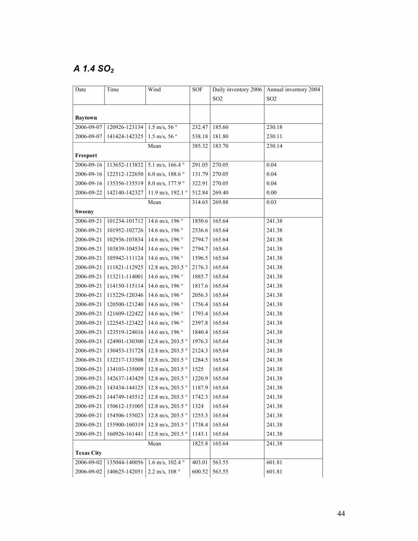
44

A 1.4 SO2 Date Time Wind SOF Daily inventory 2006 Annual inventory 2004 SO2 SO2

Baytown

2006-09-07 120926-123134 1.5 m/s, 56 ° 232.47 185.60 230.18 2006-09-07 141424-142325 1.5 m/s, 56 ° 538.18 181.80 230.11

Mean 385.32 183.70 230.14 Freeport

2006-09-16 113652-113832 5.1 m/s, 166.4 ° 291.05 270.05 0.04 2006-09-16 122512-122650 6.0 m/s, 188.6 ° 131.79 270.05 0.04 2006-09-16 135356-135519 8.0 m/s, 177.9 ° 322.91 270.05 0.04 2006-09-22 142140-142327 11.9 m/s, 192.1 ° 512.84 269.40 0.00

Mean 314.65 269.88 0.03 Sweeny

2006-09-21 101234-101712 14.6 m/s, 196 ° 1850.6 165.64 241.38 2006-09-21 101952-102726 14.6 m/s, 196 ° 2536.6 165.64 241.38 2006-09-21 102936-103834 14.6 m/s, 196 ° 2794.7 165.64 241.38 2006-09-21 103839-104534 14.6 m/s, 196 ° 2794.7 165.64 241.38 2006-09-21 105942-111124 14.6 m/s, 196 ° 1596.5 165.64 241.38 2006-09-21 111821-112925 12.8 m/s, 203.5 ° 2176.3 165.64 241.38 2006-09-21 113211-114001 14.6 m/s, 196 ° 1885.7 165.64 241.38 2006-09-21 114150-115114 14.6 m/s, 196 ° 1817.6 165.64 241.38 2006-09-21 115229-120346 14.6 m/s, 196 ° 2056.3 165.64 241.38 2006-09-21 120500-121240 14.6 m/s, 196 ° 1756.4 165.64 241.38 2006-09-21 121609-122422 14.6 m/s, 196 ° 1793.4 165.64 241.38 2006-09-21 122545-123422 14.6 m/s, 196 ° 2397.8 165.64 241.38 2006-09-21 123519-124016 14.6 m/s, 196 ° 1840.4 165.64 241.38 2006-09-21 124901-130300 12.8 m/s, 203.5 ° 1976.3 165.64 241.38 2006-09-21 130453-131728 12.8 m/s, 203.5 ° 2124.3 165.64 241.38 2006-09-21 132217-133508 12.8 m/s, 203.5 ° 1284.5 165.64 241.38 2006-09-21 134103-135009 12.8 m/s, 203.5 ° 1525 165.64 241.38 2006-09-21 142637-143429 12.8 m/s, 203.5 ° 1220.9 165.64 241.38 2006-09-21 143434-144125 12.8 m/s, 203.5 ° 1187.9 165.64 241.38 2006-09-21 144749-145512 12.8 m/s, 203.5 ° 1742.3 165.64 241.38 2006-09-21 150612-151005 12.8 m/s, 203.5 ° 1324 165.64 241.38 2006-09-21 154506-155023 12.8 m/s, 203.5 ° 1255.3 165.64 241.38 2006-09-21 155900-160319 12.8 m/s, 203.5 ° 1738.4 165.64 241.38 2006-09-21 160926-161441 12.8 m/s, 203.5 ° 1143.1 165.64 241.38

Mean 1825.8 165.64 241.38 Texas City

2006-09-02 135044-140056 1.6 m/s, 102.4 ° 403.01 563.55 601.81 2006-09-02 140625-142051 2.2 m/s, 108 ° 600.52 563.55 601.81

45

2006-09-14 105438-111147 4.0 m/s, 117 ° 851.5 581.42 601.81 2006-09-14 112802-114710 4.0 m/s, 117 ° 956.41 581.42 601.81 2006-09-20 102220-102734 6.3 m/s, 67.5 ° 1036.4 595.86 601.81 2006-09-20 104510-105219 6.3 m/s, 67.5 ° 1044 595.86 601.81 2006-09-20 110920-112112 6.3 m/s, 67.5 ° 1272.6 595.86 601.81 2006-09-20 120452-121253 6.3 m/s, 67.5 ° 1018.6 595.86 601.81 2006-09-20 124948-125911 6.3 m/s, 67.5 ° 1276.6 595.86 601.81 2006-09-20 132407-133216 6.3 m/s, 67.5 ° 1270.2 595.86 601.81 2006-09-20 140314-141224 5.7 m/s, 75 ° 1192.9 595.86 601.81 2006-09-20 144241-144936 4.3 m/s, 98.5 ° 1015.2 595.86 601.81 2006-09-20 153052-153900 4.3 m/s, 98.5 ° 952.31 595.86 601.81 2006-09-20 160604-161316 4.3 m/s, 98.5 ° 999.37 595.86 601.81 2006-09-20 163954-164639 4.3 m/s, 98.5 ° 1062.8 595.86 601.81

Mean 996.82 589.63 601.81

46

Appendix II. Detailed comparisons between 2006 Hourly EI and SOF Mom=Momentary emissions Min=4 hour minimum Max=4 hour maximum Mean=4 hour mean Std=4 hour standard deviation Date Time SOF Hourly inventory 2006 Mom Min Max Mean Std

Daily inventory 2006

Annual inventory 2004

Ethene

1. Allen Genoa Rd

2006-08-30 105705-110401 59.676 0.36 0.33 0.49 0.4 0.06 4.232181 1.346469 2006-08-30 132657-133424 105.05 0 0 0 0 0 3.382232 1.331129 2006-09-13 153846-154556 111.42 0.38 0.31 0.43 0.38 0.04 6.478974 2.038774

2. Davison Street

2006-08-30 110321-110859 138.39 0.26 0.19 0.3 0.25 0.04 16.475639 8.837804 2006-08-30 131201-132401 170.57 0 0 0 0 0 12.815598 8.167531 2006-09-13 152330-152847 114.58 0 0 0 0 0 7.96766 5.229198

3. Deer Park

2006-08-30 111058-111530 401.14 0.35 0.35 1.32 0.9 0.37 4.317818 3.261628 2006-08-30 130148-130741 279.44 1.32 0.38 1.32 0.82 0.33 4.164815 3.261628 2006-09-13 150946-151531 105.39 1.53 1.33 1.85 1.52 0.2 4.11172 3.261628

4. Battelground Rd WE

2006-08-30 111647-111947 73.919 3.47 3.47 4.43 4.18 0.41 12.108042 1.598133 2006-09-13 150112-150614 157.92 2.21 2.21 2.27 2.25 0.02 14.921539 5.496641

Battleground Rd NS

2006-08-31 114943-120918 254.28 6.1 6.1 8.77 7.85 1.05 55.883958 36.207143 2006-08-31 121844-123434 276.42 6.1 6.1 8.77 7.85 1.05 57.338052 36.207143 2006-08-31 105359-111214 158.82 6.34 5.7 6.82 6.33 0.41 46.526419 14.33718 2006-08-31 125215-131029 95.139 8.53 8 8.77 8.39 0.29 54.497602 32.912598 2006-09-14 143518-150033 479.82 10.2 7.56 11.9 9.65 1.6 69.983313 36.207143 2006-09-14 153654-160244 264.92 7.65 5.47 10.7 7.54 1.96 67.592885 33.900913 2006-09-14 160823-163610 437.32 7.65 5.47 10.7 7.54 1.96 67.592885 33.900913

5. Miller Cutoff Rd

2006-08-30 111935-112342 114.74 6.27 5.93 6.27 6.09 0.14 16.995358 30.174748 2006-09-13 145523-150126 362.68 0.82 0.45 4.13 2.25 1.63 23.424051 28.404271

6. Sens Rd

2006-08-30 112342-112645 52.491 0 0 0 0 0 2.757284 3.294545

7. Baytown

2006-08-30 112645-113500 69.728 3.44 3.44 3.79 3.62 0.14 10.339925 6.621302

47

2006-09-07 122202-123633 47.337 2.93 2.93 3.78 3.29 0.35 10.168014 6.621302 2006-09-13 144844-145409 104.41 12.8 12.1 12.8 12.3 0.25 20.257358 6.621302

8. Mt. Belvieu

2006-08-30 113203-114235 354.03 19.8 19.7 20.2 19.9 0.2 78.769235 44.845284 2006-08-30 121556-122843 275.13 19.8 19.7 20.2 19.9 0.2 78.769235 44.845284

HSC without Mt. Belvieu

2006-08-30 105336-113435 966.72 14.7 14.7 16 15.3 0.48 61.962587 55.172001 2006-08-30 122443-133757 904.59 16 13.7 16 14.7 0.88 61.947741 55.172001 2006-09-13 143954-154606 985.34 17.6 16.6 20.4 18.7 1.64 81.75886 55.156661

HSC with Channelview

2006-08-30 121532-133757 1187.5 36.4 33.3 36.4 35.1 1.22 147.821752 111.857821 2006-08-30 105336-114810 1398.3 35.1 35.1 36.8 36 0.58 148.048235 111.873161

Channelview

2006-08-31 164824-170305 46.268 0.68 0.68 0.83 0.74 0.06 7.336439 11.855876 2006-08-31 175645-181336 22.751 0.68 0.68 0.88 0.79 0.08 7.336439 11.855876

Propene

2. Davison Street

2006-08-30 110321-110859 147.6 0.69 0.5 0.8 0.65 0.11 11.088701 15.721673 2006-09-13 152847-154100 115.18 0.49 0.49 0.54 0.51 0.02 1.942632 15.721673

3. Deer Park

2006-08-30 111058-111530 710.17 2.16 2.16 4.93 3.94 1.13 13.573359 7.548861 2006-08-30 130148-130741 895.21 4.93 4.6 4.93 4.83 0.13 13.393708 7.527575 2006-09-13 150946-151531 245.8 1.8 1.62 2.13 1.81 0.19 8.785302 7.548861

4. Battleground WE

2006-08-30 111647-111947 144.53 2.18 2.18 2.19 2.18 0 25.92126 18.086466 2006-09-13 150112-150614 1010.3 11.5 8.88 19.6 14.8 4.68 74.076036 30.354554

Battleground Rd NS

2006-08-31 113741-120918 683.61 56 55.2 60.7 57.8 2.29 136.828565 80.771433 2006-08-31 121844-123434 2294.6 56 55.2 60.7 57.8 2.29 136.808371 80.696477 2006-08-31 125215-130413 237.47 56.1 50.7 61.2 55.7 3.77 127.890357 80.486078 2006-09-14 143518-150033 1319.8 29.2 21.2 29.2 24.4 3.29 114.831051 80.696477

5. Miller Cutoff Rd

2006-08-30 111935-112342 289.2 44.1 42.5 44.1 43.1 0.64 92.692476 14.811834 2006-08-30 124648-125018 235.49 0.01 0.01 0.01 0.01 0 5.271131 12.934121 2006-09-13 145523-150126 234.48 0.18 0.18 33.5 20.1 14.1 7.144036 2.053526

6. Sens Rd

2006-08-30 112342-112645 227.15 0 0 0 0 0 0.020194 0

7. Baytown

2006-08-30 123153-123603 358.7 18.3 16.4 18.3 17.5 0.69 29.649757 51.328658 2006-09-07 122202-123633 177.39 16 13.7 16 15 0.88 30.069133 51.328658

HSC winthout Mt. Belvieu

2006-08-30 105336-113435 1837.5 66.5 66.3 66.9 66.6 0.19 167.207587 112.336635 2006-09-13 144350-154534 1837.5 47.2 47.2 86.2 69.3 14.4 153.371005 111.934394

48

HSC with Channelview

2006-08-30 105336-114810 1922.9 82.6 82 82.8 82.4 0.3 215.807857 144.925955

Alkanes

1. Allen Genoa Rd

2006-09-13 122512-124109 1067.4 7.1 6.83 7.1 6.97 0.11 131.943564 11.704439

2. Davison Strret

2006-09-13 121916-122515 3076 42.2 42.1 42.2 42.2 0.04 288.7722 68.250098

3. Deer Park

2006-09-13 121255-121911 3686.9 8.12 8.12 8.46 8.26 0.13 140.298517 76.357138

4. Battleground WE

2006-09-13 120933-121305 1636.1 4.11 3.83 4.6 4.26 0.31 69.019362 38.631609

5. Miller Cutoff Rd

2006-09-13 120620-120908 595.1 5.2 0.9 5.2 3.71 1.67 13.172031 9.507327

6. Sens Rd

2006-09-13 120043-120302 752.77 0 0 2.78 0.69 1.2 14.32017 10.696204

7. Baytown

2006-08-31 151350-152352 1023.6 66.9 63.6 67.8 66.3 1.6 271.137718 74.75242 2006-09-13 115313-120025 1484.4 118 118 125 122 2.51 349.031138 75.748442

HSC without Mt. Belvieu

2006-09-13 115326-124109 11674 184 184 190 188 1.98 1005.527845 290.895258

NO2

Baytown

2006-08-28 112020-114516 501.98 210 210 221 215 4.28 608.380075 871.374718 2006-08-28 121432-123212 71.285 221 209 221 215 4.56 608.070263 870.654228 2006-08-28 123524-125407 293.47 217 209 217 213 2.62 607.940491 870.654228 2006-08-28 125735-131738 381.34 217 209 217 213 2.62 607.940491 870.654228 2006-08-28 133423-135203 878.7 212 209 213 212 1.46 608.250302 871.374718 2006-08-28 141838-143639 609.98 212 209 213 212 1.46 608.250302 871.374718 2006-08-28 143952-145845 541.37 209 164 213 200 20.9 608.985055 871.374718 2006-08-28 150302-152130 205.91 209 164 213 200 20.9 608.380075 871.374718 2006-08-28 153650-155444 239.91 213 164 214 201 21.6 608.380075 871.374718 2006-08-31 160602-162406 578.75 227 212 227 220 5.45 641.166101 871.374718 2006-08-31 163406-165220 433.49 222 209 222 215 5.55 641.166101 871.374718 2006-08-31 165918-172027 652.29 222 209 222 215 5.55 641.166101 871.374718 2006-09-04 164614-173258 245.32 229 228 229 229 0.31 675.028599 871.382339 2006-09-07 120925-131106 381.56 263 252 265 259 5.2 666.81152 871.374718 2006-09-07 141235-143934 460.82 252 252 299 277 19.5 666.81152 871.374718 2006-09-07 163947-171436 625.76 299 263 299 275 14.1 666.773721 871.374718 2006-09-07 173106-175354 432.83 257 257 269 263 4.93 640.583946 782.76697 2006-09-07 175801-181804 442.48 263 263 274 269 4.76 666.773721 871.374718

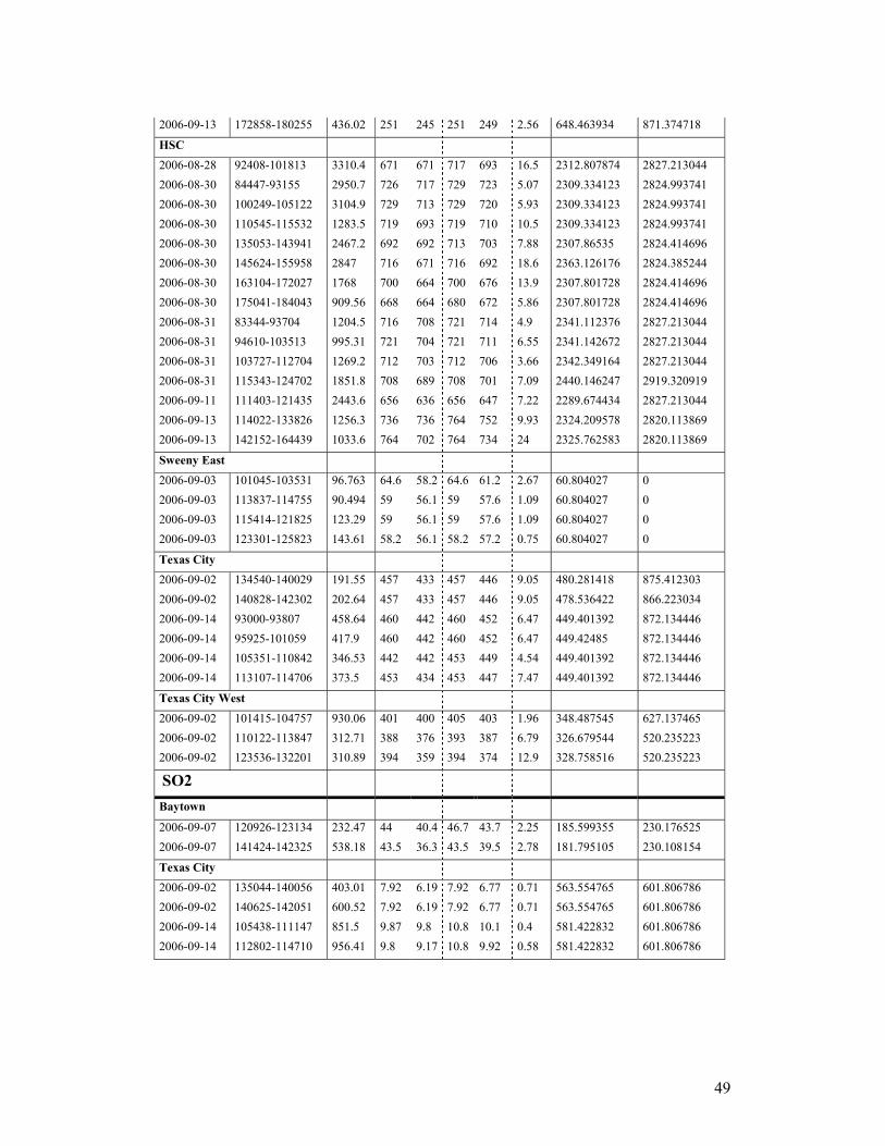
49

2006-09-13 172858-180255 436.02 251 245 251 249 2.56 648.463934 871.374718

HSC

2006-08-28 92408-101813 3310.4 671 671 717 693 16.5 2312.807874 2827.213044 2006-08-30 84447-93155 2950.7 726 717 729 723 5.07 2309.334123 2824.993741 2006-08-30 100249-105122 3104.9 729 713 729 720 5.93 2309.334123 2824.993741 2006-08-30 110545-115532 1283.5 719 693 719 710 10.5 2309.334123 2824.993741 2006-08-30 135053-143941 2467.2 692 692 713 703 7.88 2307.86535 2824.414696 2006-08-30 145624-155958 2847 716 671 716 692 18.6 2363.126176 2824.385244 2006-08-30 163104-172027 1768 700 664 700 676 13.9 2307.801728 2824.414696 2006-08-30 175041-184043 909.56 668 664 680 672 5.86 2307.801728 2824.414696 2006-08-31 83344-93704 1204.5 716 708 721 714 4.9 2341.112376 2827.213044 2006-08-31 94610-103513 995.31 721 704 721 711 6.55 2341.142672 2827.213044 2006-08-31 103727-112704 1269.2 712 703 712 706 3.66 2342.349164 2827.213044 2006-08-31 115343-124702 1851.8 708 689 708 701 7.09 2440.146247 2919.320919 2006-09-11 111403-121435 2443.6 656 636 656 647 7.22 2289.674434 2827.213044 2006-09-13 114022-133826 1256.3 736 736 764 752 9.93 2324.209578 2820.113869 2006-09-13 142152-164439 1033.6 764 702 764 734 24 2325.762583 2820.113869

Sweeny East

2006-09-03 101045-103531 96.763 64.6 58.2 64.6 61.2 2.67 60.804027 0 2006-09-03 113837-114755 90.494 59 56.1 59 57.6 1.09 60.804027 0 2006-09-03 115414-121825 123.29 59 56.1 59 57.6 1.09 60.804027 0 2006-09-03 123301-125823 143.61 58.2 56.1 58.2 57.2 0.75 60.804027 0

Texas City

2006-09-02 134540-140029 191.55 457 433 457 446 9.05 480.281418 875.412303 2006-09-02 140828-142302 202.64 457 433 457 446 9.05 478.536422 866.223034 2006-09-14 93000-93807 458.64 460 442 460 452 6.47 449.401392 872.134446 2006-09-14 95925-101059 417.9 460 442 460 452 6.47 449.42485 872.134446 2006-09-14 105351-110842 346.53 442 442 453 449 4.54 449.401392 872.134446 2006-09-14 113107-114706 373.5 453 434 453 447 7.47 449.401392 872.134446

Texas City West

2006-09-02 101415-104757 930.06 401 400 405 403 1.96 348.487545 627.137465 2006-09-02 110122-113847 312.71 388 376 393 387 6.79 326.679544 520.235223 2006-09-02 123536-132201 310.89 394 359 394 374 12.9 328.758516 520.235223

SO2

Baytown

2006-09-07 120926-123134 232.47 44 40.4 46.7 43.7 2.25 185.599355 230.176525 2006-09-07 141424-142325 538.18 43.5 36.3 43.5 39.5 2.78 181.795105 230.108154

Texas City

2006-09-02 135044-140056 403.01 7.92 6.19 7.92 6.77 0.71 563.554765 601.806786 2006-09-02 140625-142051 600.52 7.92 6.19 7.92 6.77 0.71 563.554765 601.806786 2006-09-14 105438-111147 851.5 9.87 9.8 10.8 10.1 0.4 581.422832 601.806786 2006-09-14 112802-114710 956.41 9.8 9.17 10.8 9.92 0.58 581.422832 601.806786

50