comparison of novel phase i clinical trial...
TRANSCRIPT

COMPARISON OF NOVEL PHASE I CLINICAL TRIAL DESIGNS BASED ON TOXICITY PROBABILITY INTERVALS
by
Yi Yao
MA, Shanghai University of Sports, China, 2012
MSW, University of Pittsburgh, 2015
Submitted to the Graduate Faculty of
the Department of Biostatistics
Graduate School of Public Health in partial fulfillment
of the requirements for the degree of
Master of Science
University of Pittsburgh
2017

ii
UNIVERSITY OF PITTSBURGH GRADUATE SCHOOL OF PUBLIC HEALTH
This thesis was presented by
Yi Yao
It was defended on
April 12, 2017
and approved by
Thesis Advisor: Hong Wang, PhD
Research Assistant Professor Department of Biostatistics
Graduate School of Public Health University of Pittsburgh
Committee Member:
Yan Lin, PhD Research Associate Professor Department of Biostatistics
Graduate School of Public Health University of Pittsburgh
Committee Member: Kaleb Z. Abebe, PhD Associate Professor
Department of Medicine, Biostatistics School of Medicine and Graduate School of Public Health
University of Pittsburgh
Committee Member: Seo Young Park, PhD
Assistant Professor Department of Medicine, Biostatistics
School of Medicine and Graduate School of Public Health University of Pittsburgh

iii
Copyright © by Yi Yao 2017

iv
ABSTRACT
Phase I clinical trial based on toxicity probability intervals is a new class of dose-finding designs
characterized by integrating the concept of intervals, instead of point estimates, in detection of the
maximum tolerated dose. The purpose of this article is to explore and compare the performance of
three novel designs including the two-parameter logistic regression model with categorized
posterior probability design (LRcat), the modified toxicity probability interval design (mTPI) and
the Bayesian optimal interval design (BOIN). A thorough numeric study with eight potential
scenarios was conducted to examine critical operating characteristics. Robustness of the novel
designs to the change in the target interval width and mis-specified priors was investigated in a
sensitivity analysis following the simulation study. In addition, we also retrospectively analyzed a
recent cancer phase I clinical trial to explore the performance of these designs in real-world
application
The results of our analysis showed that interval-based designs perform comparably to a
traditional CRM design using posterior mean to define MTD in most scenarios. LRcat is more
flexible than CRM and demonstrates robustness to the varying target toxicity interval. BOIN is
safer than other designs and allocates less patients to overly-toxic levels. mTPI is more likely to
allocate patients to suboptimal doses when the true MTD resides at the lowest/highest doses and
performs poorly when the target interval is asymmetric.
Hong Wang, PhD
COMPARISON OF NOVEL PHASE I CLINICAL TRIAL DESIGNS BASED ON TOXICITY PROBABILITY INTERVALS
Yi Yao, MS
University of Pittsburgh, 2017

v
PUBLIC HEALTH SIGNIFICANCE
Phase I cancer clinical trials are the indispensable step for the development of anticancer therapies.
With the widespread application of phase I clinical trials, researchers and clinical investigators
need up-to-date information about newly-developed phase I clinical trial methods. By providing
the comparison result for a group of innovative phase I trial designs, our study facilitates choice
of dose-finding method and leads to more efficient and ethical drug development to conquer cancer
epidemic.

vi
TABLE OF CONTENTS
1.0 INTRODUCTION............................................................................................................. 1
2.0 PHASE I CLINICAL TRIAL DESIGNS BASED ON TOXICITY POSTERIOR
INTERVALS ................................................................................................................................. 4
2.1 LRCAT DESIGN .................................................................................................... 4
2.2 MTPI DESIGN ...................................................................................................... 6
2.3 BOIN DESIGN ..................................................................................................... 8
3.0 NUMERICAL STUDY ................................................................................................... 10
3.1 SIMULATION SETTING ................................................................................ 10
3.2 EVALUATION METRICS............................................................................... 12
3.3 RESULTS ........................................................................................................... 13
3.3.1 Selection percentage of the MTD ................................................................. 13
3.3.2 Patient allocation, risk of over-dosing and under-dosing .......................... 17
3.3.3 Toxicity ........................................................................................................... 18
3.4 SENSITIVITY ANALYSIS .............................................................................. 19
3.4.1 Sensitivity to interval width .......................................................................... 19
3.4.2 Sensitivity of LRcat and CRM to mis-specified priors .............................. 22
4.0 REANALYSIS OF A RECENT ONCOLOGICAL CLINICAL TRIAL .................. 25
5.0 COMPUTATION ............................................................................................................ 29
6.0 DISCUSSION .................................................................................................................. 30
APPENDIX A. DOSE-FINDING SPREADSHEETS .............................................................. 33

vii
APPENDIX B: R CODE ............................................................................................................ 35
BIBLIOGRAPHY ....................................................................................................................... 43

viii
LIST OF TABLES
Table 1. Scenarios for simulation study. ....................................................................................... 11
Table 2. Prior specification for CRM and LRcat .......................................................................... 12
Table 3. Interval-based designs with symmetric target intervals of varying width. ..................... 21
Table 4. Interval-based designs with asymmetric target intervals ................................................ 22
Table 5. Comparison of CRM and LRcat in Scenario 7 with different priors .............................. 24
Table 6. The original example trial ............................................................................................... 26
Table 7. Results of the reanalysis of the example trial ................................................................. 27

ix
LIST OF FIGURES
Figure 1. Dose assignment scheme for LRcat design and mTPI design ......................................... 9
Figure 2. Dose-toxicity relationships of the eight simulation scenarios. ...................................... 11
Figure 3. Selection percentage of MTD ........................................................................................ 15
Figure 4. Patient allocation ........................................................................................................... 16
Figure 5. Risk of over-dosing and risk of under-dosing ............................................................... 18
Figure 6. Average proportion of toxicity. ..................................................................................... 19
Figure 7. The median and 95% credible interval of prior probability of DLT for CRM and LRcat.
....................................................................................................................................................... 23

1
1.0 INTRODUCTION
Phase I clinical trials serve as a vital part and generally the first-in-human studies in translating
laboratory research into clinical practice. A phase I clinical trial in oncology aims to identify the
maximum tolerated dose (MTD). For cytotoxic anticancer agents, the rationale of using MTD as
the primary endpoint based on the assumption: the treatment efficacy increases monotonically with
the probability of toxicity [1]. Therefore, by determining the MTD, oncological phase I clinical
trials provide the most efficacious dose of a treatment with acceptable side effects. In 1997, the
American Society of Clinical Oncology (ASCO) published a policy statement on the centrality of
phase I clinical trials to the process of discovering anticancer agents and brought up the prosperity
in the development and application of early-phase cancer trials [2].
Numerous dose-finding designs for phase I clinical trials have been invented over the past
few decades. Most of these designs fall into one of the two major categories: algorithmic (rule-
based) designs or model-based designs. Algorithmic designs are guided by predetermined rules
and the dose limiting toxicity (DLT) information obtained from the last cohort of patients in the
trial, whereas model-based designs use explicit parametric models and cumulative DLT
information throughout the trial. Examples of algorithmic designs include: the traditional “3+3”
design and its variations [3], the accelerated titration design proposed by Simon et al, Ivanova’s
up-and-down design [4], among others. The most representative model-based designs include the
continual reassessment method (CRM) [5] and its extensions, and the dose escalation with
overdose control (EWOC) design [6].

2
Rule-based designs are well-recognized for their simplicity and transparency in
application, but their slow convergence to the true MTD and lack of a prespecified target toxicity
rate are indisputable drawbacks. On the other hand, model-based designs are praised for more
rapid dose escalation and a complete use of cumulative trial information, but are frequently
criticized for aggressiveness, ambiguous prior specifications and complex computations [7].
Confronted with the trade-offs between the two bodies of designs, researchers resort to seeking
new designs that are more flexible, utilize more information, and yet do not compromise good
operating characteristic and simplicity.
During the past decade, clinical researchers have witnessed the development of a new class
of designs that utilize toxicity probability intervals, instead of a single point estimate, to determine
the MTD. Ji et al. proposed a dose-finding method named toxicity posterior intervals (TPI) design.
This design partitions beta posterior distributions for the toxicity probabilities of the current dose
into three intervals. The toxicity intervals are labeled as high, acceptable, and low toxicity, each
associated with the corresponding dose-assignment decision for future patients [9]. TPI design was
further extended to a modified toxicity probability interval (mTPI) design, which depends the
decision rules on maximizing unit probability mass (UPM) of the intervals [10]. Following in the
footsteps of Ji and his colleagues, Yuan et al. proposed the Bayesian optimal interval (BOIN) in
2016. The design derives the boundaries of the target toxicity probability interval from a Bayesian
decision making process rather than solely relying on a physician’s judgement. Like the mTPI
design, dose assignments in the BOIN design is determined by the location of the current toxicity
rate with respect to the interval boundaries [11]. Meanwhile, Neuenschwander et al. introduced a
design that is similar to TPI but inherits many features of a CRM procedure. The design, referred
to as LRcat in the paper, adopts a two-parameter logistic model to obtain the posterior distribution

3
of toxicity probability. After each experiment, the posterior distributions are summarized for each
dose by the probability of four categories: under-dosing, target, excessive toxicity, unacceptable
toxicity. Then the next dose is recommended as the dose which has the maximum probability of
target interval [11]. As is in the case with CRM design, LRcat design has a “jumping” nature in
dose assignment. A variation of LRcat design (LRcat25) guides dose selection by maximizing the
probability of target interval while controlling the risk of overdosing at 25%. Details about these
innovative designs will be further discussed in Section 2.
Our study will focus on the newly-developed interval-based designs mentioned above. The
primary objective of this article is to explore the operating characteristics of LRcat /LRcat25, mTPI
and BOIN relative to the CRM in numerical study with various potential scenarios. We would like
to see how robust are the three designs to a varying target interval width, and how sensitive is
LRcat, comparing to CRM, to a mis-specified prior. In addition, we applied a post-hoc dose-
escalation analysis using the real-life data from a recent cancer clinical trial to further investigate
the application of these innovative designs. This study is innovative as no head-to-head
comparison of these three designs, to our best knowledge, has been carried out ever before.
Starting in Section 2, we provide an overview of newly developed statistical designs for
phase I cancer trial, LRcat, mTPI and BOIN. Section 3 presents the simulation study and the
sensitivity analysis. In Section 4, a recent cancer phase I clinical trial will be reanalyzed via each
of the novel designs. Finally, a discussion about practical implications of these designs will be
given in Section 6.

4
2.0 PHASE I CLINICAL TRIAL DESIGNS BASED ON TOXICITY POSTERIOR INTERVALS
Researchers hold different opinions about optimalizing phase I clinical trial designs.
Neuenswander suggested that plausible dose recommendations should use more informative
posterior summaries and more flexible models [11]. He proposed the LRcat design, rendering it
an extension of the CRM design to incorporate posterior intervals for the probabilities of DLT.
However, from the perspective of application, designs that are easy to understand and implement
for investigators are more favorable. This rationale leads to the development of mTPI and BOIN.
2.1 LRCAT DESIGN
Suppose a trial has J doses and we aim at identifying the MTD from a set of doses 𝑑𝑑1 < 𝑑𝑑2 < ⋯ <
𝑑𝑑𝐽𝐽. The probability of a DLT at dose d is denoted as 𝜋𝜋𝜃𝜃(𝑑𝑑) and is described by the logistic model:
logit[𝜋𝜋𝜃𝜃(𝑑𝑑𝑖𝑖; 𝛼𝛼,𝛽𝛽)] = log𝛼𝛼 + 𝛽𝛽 ∙ log(𝑑𝑑𝑖𝑖 𝑑𝑑∗⁄ ) (1)
where 𝛼𝛼,𝛽𝛽 > 0, and 𝑑𝑑∗ is a reference dose allowing log(𝛼𝛼) to be the log-odds of toxicity
when 𝑑𝑑𝑖𝑖 = 𝑑𝑑∗ . A bivariate normal prior for (log𝛼𝛼, log𝛽𝛽) is assumed:
log(𝜽𝜽) = �log𝛼𝛼log𝛽𝛽� ~ 𝐵𝐵𝐵𝐵𝐵𝐵��
𝜇𝜇1𝜇𝜇2� ,𝜮𝜮� , 𝜮𝜮 = � 𝜎𝜎12 𝜌𝜌𝜎𝜎1𝜎𝜎2
𝜌𝜌𝜎𝜎1𝜎𝜎2 𝜎𝜎22�
Neuenschwander postulated that placing a bivariate lognormal prior on the two parameters
makes the model more flexible than a one-parameter power or logistic model commonly used in
CRM design. An noninformative prior distribution for LRcat could be derived by matching
quantiles with a minimally informative beta distribution as defined in [11]. Neuenschwander et al.
also recommended the use of informative priors whenever is available.

5
The posterior distribution is then
𝑓𝑓(𝛼𝛼,𝛽𝛽|𝑦𝑦1, … ,𝑦𝑦𝑛𝑛) ∝ 𝑓𝑓(𝛼𝛼,𝛽𝛽)𝐿𝐿(𝛼𝛼,𝛽𝛽;𝑦𝑦1, … ,𝑦𝑦𝑛𝑛)
where 𝑓𝑓(𝛼𝛼,𝛽𝛽) is the joint prior distribution and 𝐿𝐿(𝛼𝛼,𝛽𝛽;𝑦𝑦1, … ,𝑦𝑦𝑛𝑛) is the likelihood
function.
A Gibbs sampling procedure is then applied to elicit posterior samples of (𝛼𝛼,𝛽𝛽), and the
posterior distribution of DLT at each dose level is obtained from the inversed model function (1)
𝜋𝜋𝜃𝜃(𝑑𝑑𝑖𝑖; 𝛼𝛼,𝛽𝛽) =exp (log𝛼𝛼 + 𝛽𝛽 ∙ log(𝑑𝑑 𝑑𝑑∗⁄ ))
1 + exp (log𝛼𝛼 + 𝛽𝛽 ∙ log(𝑑𝑑 𝑑𝑑∗⁄ ))
Next, the computed posterior distribution of 𝜋𝜋𝜃𝜃(𝑑𝑑𝑖𝑖) is partitioned by three cutpoints
(0.20, 0.35, 0.60) and is summarized into
Under-dosing 𝑃𝑃{𝜋𝜋𝜃𝜃(𝑑𝑑) ∈ (0, 0.20]} Targeted toxicity 𝑃𝑃{𝜋𝜋𝜃𝜃(𝑑𝑑) ∈ (0.20, 0.35]} Excessive toxicity 𝑃𝑃{𝜋𝜋𝜃𝜃(𝑑𝑑) ∈ (0.35, 0.60]} Unacceptable toxicity 𝑃𝑃{𝜋𝜋𝜃𝜃(𝑑𝑑) ∈ (0.60, 1.00]}
These intervals are subject to change based on the specific setting of the study [12]. The
dose recommended for the next cohort of patients is the dose that has a maximal posterior
probability for the target interval. Figure 1 shows a flow chart illustrating the dose escalation
scheme of LRcat design.
There are two variations of LRcat design. LRcat25 takes patient safety as the primary
concern and enforces an overdose control on excessive and unacceptable toxicity intervals. The
probability of the last two toxicity intervals are required to be less than 0.25.
𝑠𝑠𝑠𝑠𝑠𝑠𝑠𝑠𝑠𝑠𝑠𝑠 𝑎𝑎 𝑑𝑑𝑑𝑑𝑠𝑠𝑠𝑠 𝑠𝑠𝑠𝑠𝑙𝑙𝑠𝑠𝑠𝑠 𝑓𝑓𝑑𝑑𝑓𝑓 𝑠𝑠𝑎𝑎𝑠𝑠ℎ 𝑝𝑝𝑎𝑎𝑠𝑠𝑝𝑝𝑠𝑠𝑝𝑝𝑠𝑠 𝑠𝑠. 𝑠𝑠.
𝑃𝑃{𝜋𝜋𝜃𝜃(𝑑𝑑) ∈ (0.35, 0.60]} + 𝑃𝑃{𝜋𝜋𝜃𝜃(𝑑𝑑) ∈ (0.60, 1.00]} < 0.25

6
This criteria is similar to the escalation with overdose control (EWOC) design introduced
by Babb and his colleagues which restricts the predicted proportion of patients who receive an
overdose to a feasibility bound [6].
Another variation adapts a fully Bayesian decision analytic approach using a formal loss
function:
where 𝑠𝑠𝑘𝑘 represents the distance of the corresponding interval from the true MTD. The
optimal decision is the one that minimizes the corresponding Bayes risk: 𝐵𝐵𝑎𝑎𝑦𝑦𝑠𝑠𝑠𝑠 𝑓𝑓𝑝𝑝𝑠𝑠𝑟𝑟 =
𝑠𝑠1𝑃𝑃{𝜋𝜋𝜃𝜃(𝑑𝑑) ∈ (0, 0.20]} + 𝑠𝑠2𝑃𝑃{𝜋𝜋𝜃𝜃(𝑑𝑑) ∈ (0.20, 0.35]} + 𝑠𝑠3𝑃𝑃{𝜋𝜋𝜃𝜃(𝑑𝑑) ∈ (0.35, 0.60]} +
𝑠𝑠4𝑃𝑃{𝜋𝜋𝜃𝜃(𝑑𝑑) ∈ (0.60, 1.00]} [11]. The original LRcat design has an implicit 1-0-1-1 loss function.
If a more conservative dose escalation design is sought, loss functions like 1-0-1-2 and 1-0-2-4
could lower the risk of selecting doses that are too toxic.
2.2 MTPI DESIGN
Let 𝑝𝑝𝑇𝑇 denote the target toxicity probability and 𝑝𝑝𝑖𝑖 the toxicity probability for dose 𝑝𝑝 = 1, … , 𝐽𝐽. An
equivalence interval (EI), [𝑝𝑝𝑇𝑇 − 𝜖𝜖1,𝑝𝑝𝑇𝑇 + 𝜖𝜖2] , is defined. The width of EI depends on the
phycisian’s judgement. Any dose included in the EI is considered potential candidate for the true
MTD. 𝑥𝑥𝑖𝑖 ,𝑝𝑝𝑖𝑖 represent number of patients treated and number of patients experiencing toxicity at
dose 𝑝𝑝 respectively. 𝑥𝑥’s are assumed to follow a binomial distribution
𝑓𝑓(𝑥𝑥; 𝑝𝑝, 𝑝𝑝) = �𝑝𝑝𝑥𝑥� 𝑝𝑝𝑥𝑥(1 − 𝑝𝑝)𝑛𝑛−𝑥𝑥
𝑠𝑠1 𝑝𝑝𝑓𝑓 𝜋𝜋𝜃𝜃(𝑑𝑑) ∈ (0, 0.20]
𝑠𝑠2 𝑝𝑝𝑓𝑓 𝜋𝜋𝜃𝜃(𝑑𝑑) ∈ (0.20, 0.35]
𝑠𝑠3 𝑝𝑝𝑓𝑓 𝜋𝜋𝜃𝜃(𝑑𝑑) ∈ (0.35, 0.60]
𝑠𝑠4 𝑝𝑝𝑓𝑓 𝜋𝜋𝜃𝜃(𝑑𝑑) ∈ (0.60, 1.00]
𝐿𝐿(𝜃𝜃, 𝑑𝑑) =

7
And the likelihood function is derived as
𝑠𝑠(𝑥𝑥𝑖𝑖|𝑝𝑝𝑖𝑖) ∝�𝑝𝑝𝑖𝑖𝑥𝑥𝑖𝑖
𝐽𝐽
𝑖𝑖=1
(1 − 𝑝𝑝𝑖𝑖)𝑛𝑛𝑖𝑖−𝑥𝑥𝑖𝑖
A vague conjugate beta prior is assumed: 𝑝𝑝𝑖𝑖 ~ 𝑝𝑝. 𝑝𝑝.𝑑𝑑.𝐵𝐵𝑠𝑠𝑠𝑠𝑎𝑎(1, 1). Followed from the Bayes
theorem [9]
𝑓𝑓(𝑝𝑝𝑖𝑖|𝑥𝑥𝑖𝑖) ∝ 𝑓𝑓(𝑝𝑝𝑖𝑖)𝑠𝑠(𝑥𝑥𝑖𝑖|𝑝𝑝𝑖𝑖)
𝑝𝑝𝑖𝑖|𝑥𝑥𝑖𝑖 ~ 𝑝𝑝. 𝑝𝑝. 𝑑𝑑.𝐵𝐵𝑠𝑠𝑠𝑠𝑎𝑎(1 + 𝑥𝑥𝑖𝑖, 1 + 𝑝𝑝𝑖𝑖 − 𝑥𝑥𝑖𝑖)
After obtaining the posterior distribution of 𝑝𝑝𝑖𝑖 , the unit probability mass (UPM) is
calculated for each of the three intervals partitioned by EI. UPM is defined as the probability of
the interval divided by the length of the interval [10]. For example, Let 𝐵𝐵(𝑥𝑥;𝑎𝑎, 𝑏𝑏) be the
cumulative distribution function of the Beta distribution. The UPM of EI is
𝐵𝐵(𝑝𝑝𝑇𝑇 + 𝜖𝜖2, 1 + 𝑥𝑥𝑖𝑖 , 1 + 𝑝𝑝𝑖𝑖 − 𝑥𝑥𝑖𝑖) − 𝐵𝐵(𝑝𝑝𝑇𝑇 − 𝜖𝜖1, 1 + 𝑥𝑥𝑖𝑖, 1 + 𝑝𝑝𝑖𝑖 − 𝑥𝑥𝑖𝑖) 𝜖𝜖1 + 𝜖𝜖2
One of the dose assignment decisions, escalation, stay at the same dose and de-escalation,
is chosen depending on which of the three intervals, (0, p𝑇𝑇 − 𝜖𝜖1), [𝑝𝑝𝑇𝑇 − 𝜖𝜖1, 𝑝𝑝𝑇𝑇 + 𝜖𝜖2] and (pT +
𝜖𝜖2, 1) has the largest UPM. This process repeats until a primary stopping rule (e.g. maximum
sample size) is satisfied. At the end of the trial, we use a less informative beta prior,
𝐵𝐵𝑠𝑠𝑠𝑠𝑎𝑎(0.005, 0.005), to obtain the posterior distribution. The isotonically transformed posterior
mean for each dose level is calculated and the dose level with the smallest absolute difference
between the posterior mean and the target toxicity is selected as the MTD [10].
There are two built-in safety rules for mTPI design. The first safety rule requires an early
termination of the trial when the probability of dose 1 excessing the target toxicity is over 95%.
The second one check the next dose in advance during dose escalation to prevent going to an overly

8
toxic dose [10]. Figure 1 provides a comparison of the dose-finding schemes for LRcat design and
mTPI design.
2.3 BOIN DESIGN
Both LRcat and mTPI design assume that the interval boundaries of the posterior toxicity
distribution are independent of dose level 𝑝𝑝 and the number of patient treated at dose level 𝑝𝑝. Liu
and her colleagues described a Bayesian framework to select interval boundaries based on the
accumulated toxicity information throughout the trial [12]. Following the same notations from
mTPI, �̂�𝑝𝑖𝑖 = 𝑥𝑥𝑖𝑖 𝑝𝑝𝑖𝑖⁄ denotes the observed toxicity rate at dose level 𝑝𝑝. Three point hypothesis are
formulated:
𝐻𝐻0𝑖𝑖: 𝑝𝑝𝑖𝑖 = 𝜙𝜙 𝑇𝑇ℎ𝑠𝑠 𝑠𝑠𝑐𝑐𝑓𝑓𝑓𝑓𝑠𝑠𝑝𝑝𝑠𝑠 𝑑𝑑𝑑𝑑𝑠𝑠𝑠𝑠 𝑝𝑝𝑠𝑠 𝑠𝑠ℎ𝑠𝑠 𝑀𝑀𝑇𝑇𝑀𝑀 𝐻𝐻1𝑖𝑖: 𝑝𝑝𝑖𝑖 = 𝜙𝜙1 𝑇𝑇ℎ𝑠𝑠 𝑠𝑠𝑐𝑐𝑓𝑓𝑓𝑓𝑠𝑠𝑝𝑝𝑠𝑠 𝑑𝑑𝑑𝑑𝑠𝑠𝑠𝑠 𝑝𝑝𝑠𝑠 𝑠𝑠𝑐𝑐𝑏𝑏𝑠𝑠ℎ𝑠𝑠𝑓𝑓𝑎𝑎𝑝𝑝𝑠𝑠𝑐𝑐𝑠𝑠𝑝𝑝𝑠𝑠 𝐻𝐻2𝑖𝑖: 𝑝𝑝𝑖𝑖 = 𝜙𝜙2 𝑇𝑇ℎ𝑠𝑠 𝑠𝑠𝑐𝑐𝑓𝑓𝑓𝑓𝑠𝑠𝑝𝑝𝑠𝑠 𝑑𝑑𝑑𝑑𝑠𝑠𝑠𝑠 𝑝𝑝𝑠𝑠 𝑠𝑠𝑑𝑑𝑑𝑑 𝑠𝑠𝑑𝑑𝑥𝑥𝑝𝑝𝑠𝑠
where 𝑝𝑝𝑖𝑖 is the true toxicity probability of the current dose, 𝜙𝜙 is the target toxicity
probability, 𝜙𝜙1, 𝜙𝜙2 are the toxicity probability of the highest sub-therapeutic and the lowest overly
toxic dose respectively. The prior probability of each hypothesis being true is defined as 𝜋𝜋𝑘𝑘𝑖𝑖 =
Pr(𝐻𝐻𝑘𝑘𝑖𝑖) ,𝑟𝑟 = 1,2,3. The noninformative prior probability for the hypothesis is 𝜋𝜋1𝑖𝑖 = 𝜋𝜋2𝑖𝑖 = 𝜋𝜋3𝑖𝑖 =
1 3⁄ . Let 𝜆𝜆1𝑖𝑖 and 𝜆𝜆2𝑖𝑖 respectively denote the dose escalation and de-escalation boundaries. The
probability of making incorrect decision, denoted as α(𝜆𝜆1𝑖𝑖,𝜆𝜆2𝑖𝑖), is computed based on the Bayes
theorem:
𝛼𝛼(𝜆𝜆1𝑖𝑖,𝜆𝜆2𝑖𝑖) = 𝑃𝑃𝑓𝑓(𝐻𝐻0𝑖𝑖)𝑃𝑃𝑓𝑓{(�̂�𝑝𝑖𝑖 ≤ 𝜆𝜆1𝑖𝑖) ∪ (�̂�𝑝𝑖𝑖 ≥ 𝜆𝜆2𝑖𝑖)|𝐻𝐻0𝑖𝑖}+ 𝑃𝑃𝑓𝑓(𝐻𝐻1𝑖𝑖)𝑃𝑃𝑓𝑓{�̂�𝑝𝑖𝑖 < 𝜆𝜆2𝑖𝑖|𝐻𝐻1𝑖𝑖} + 𝑃𝑃𝑓𝑓(𝐻𝐻2𝑖𝑖)𝑃𝑃𝑓𝑓{�̂�𝑝𝑖𝑖 > 𝜆𝜆1𝑖𝑖|𝐻𝐻0𝑖𝑖}
When 𝜋𝜋1𝑖𝑖 = 𝜋𝜋2𝑖𝑖 = 𝜋𝜋3𝑖𝑖, it can be shown that α(𝜆𝜆1𝑖𝑖, 𝜆𝜆2𝑖𝑖) is the likelihood-ratio hypothesis-
testing boundaries

9
𝜆𝜆1𝑖𝑖 =log �1 − 𝜙𝜙1
1 − 𝜙𝜙 �
log �𝜙𝜙(1 − 𝜙𝜙1)𝜙𝜙1(1 − ϕ)�
, 𝜆𝜆2𝑖𝑖 =log � 1 − 𝜙𝜙
1 − 𝜙𝜙2�
log �𝜙𝜙2(1 − 𝜙𝜙)𝜙𝜙(1 − 𝜙𝜙2)�
Once the interval boundaries 𝜆𝜆1𝑖𝑖, 𝜆𝜆2𝑖𝑖 are decided, the next dose is selected based on the
comparison of the current observed toxicity rate �̂�𝑝𝑖𝑖 with respect to the boundaries. If �̂�𝑝𝑖𝑖 ≤ 𝜆𝜆1𝑖𝑖, we
escalate to the next dose level; if �̂�𝑝𝑖𝑖 ≥ 𝜆𝜆2𝑖𝑖, we de-escalate the dose; and if �̂�𝑝𝑖𝑖 ∈ (𝜆𝜆1𝑖𝑖,𝜆𝜆2𝑖𝑖), we retain
the current dose [13]. The dose assignment rule of the BOIN design is clearly an adaptation of a
rule-based design. To eliminate an overly toxic dose for safety, BOIN design checks the toxicity
rate of the lowest dose to see if it exceeds the target toxicity at 95%.
In the following analysis involving BOIN, we used 𝜙𝜙1 = 0.6𝜙𝜙 𝑎𝑎𝑝𝑝𝑑𝑑 𝜙𝜙2 = 1.4𝜙𝜙, which is
recommended for general use by Liu et al. [13].
Figure 1. Comparison of dose assignment scheme for LRcat design (left) and mTPI design (right)
10
3.0 NUMERICAL STUDY
3.1 SIMULATION SETTING
We performed computer simulations on six phase I clinical designs: the traditional continual
reassessment method with power model (CRM); a modified CRM constraining dose-skipping
during escalation and only selecting doses with mean posterior probability of DLT lower than the
target toxicity (mCRM) as the MTD; and the mTPI, BOIN and LRcat designs introduced in Section
2. In addition, we add the LRcat25 (LRcat with 25% overdose control) design as a variation of
LRcat commensurable to mCRM. To obtain the operating characteristics of the six designs, 2000
trials for each scenario was simulated.
We considered a hypothetical phase I trial with seven dose levels (12.5, 25, 50, 100, 150,
200, 250) and a target toxicity rate of 30%. Assuming the desired dose is among these seven dose
levels, eight scenarios were selected to represent a broad class of potential dose-toxicity relations
(Figure 2). We specified the scenarios based on four parameters: the target toxicity and the
corresponding dose; an unacceptable toxicity rate (0.90 for steep curves and 0.65 for flat curves)
and the corresponding dose. Dose-toxicity curves generated from this method were slightly
modified to obtain more distinctive characteristics. Scenarios 1 and 8 represent two boundary
scenarios with MTD at dose level 1 and 7. When the true MTD is at dose levels 2, 4 and 6, we
considered two plausible dose-toxicity curves: a steep one indicating there is an abrupt increase of
toxicity rate just before the MTD, and a flat one indicating the toxicity rate increases steadily
throughout the trial. The maximum sample size is 36. A similar simulation setting was used in
Neuenswander’s papar [11].

11
Figure 2. Dose-toxicity relationships of the eight simulation scenarios. The horizontal line represents the target toxicity probability of 0.3.
Table 1. Scenarios for simulation study.
The CRM requires specification of a prior distribution and a set of initial guesses (skeleton)
of the toxicity probabilities for the candidate doses to be used in the trial. For CRM and mCRM,
the dose toxicity model is assumed to be empiric 𝜋𝜋𝜃𝜃(𝑑𝑑) = 𝑠𝑠𝑑𝑑𝜃𝜃 with a vague prior distribution for
log (𝜃𝜃) specified as normal with 𝜇𝜇 = 0 and 𝜎𝜎2 = 1.342 [5]. The skeleton 𝑠𝑠𝑑𝑑 is calibrated using the
algorithm elaborated in [14]. For the two-parameter logistic regression model in LRcat and
LRcat25, we adapted the prior bivariate normal distributions for log (α) and log (β) derived in
Neuenschwander et al’s paper from the quantile-based method [11]. To make the comparison
Dose 12.5 25 50 100 150 200 250 Scenario 1 0.30, 0.41, 0.53, 0.61, 0.71, 0.76, 0.84 Scenario 2 0.13, 0.30, 0.55, 0.76, 0.84, 0.90, 0.92 Scenario 3 0.24, 0.30, 0.38, 0.53, 0.66, 0.71, 0.79 Scenario 4 0.01, 0.04, 0.09, 0.30, 0.52, 0.65, 0.73 Scenario 5 0.15, 0.17, 0.23, 0.30, 0.36, 0.44, 0.51 Scenario 6 0.01, 0.02, 0.02, 0.06, 0.14, 0.30, 0.56 Scenario 7 0.03, 0.04, 0.10, 0.17, 0.23, 0.30, 0.37 Scenario 8 0.01, 0.03, 0.07, 0.10, 0.14, 0.17, 0.30 NOTE: The target dose is in boldface.

12
between CRM and LRcat more sensible, we used two pairs of matched priors as depicted in Table
2 and Figure 7. The first pair of priors (A) assumes the MTD at the highest dose level and prior
(B) assumes the MTD at the second dose level. Prior (A) is used in the simulation study.
Table 2. Prior specification for CRM and LRcat
3.2 EVALUATION METRICS
A well-founded phase I trial design should lead to accurate estimation of the MTD while
concentrating dose assignments at or closely below the MTD. It also should minimize dose
assignments at suboptimal dose levels and associate greater penalty with overdosing compared to
under-dosing [6]. In light of these criteria, we considered the following five metrics to measure
the performance of the designs:
i. Distribution of the selection percentages of the MTD. Instead of using a single
percentage of correct selection (PCS) on the true MTD dose level, we choose to
exhibit the percentage of selecting the dose as the MTD for each dose levels. When
PCS may give a similar conclusion about two designs, this metrics facilitates relative
evaluation of suboptimal dose assignments.
ii. Distribution of number of patients treated on dose. This metrics presents the average
number of patients treated at each dose across the simulated trials. The number
treated at or above the true MTD will raise particular concerns.
iii. The risk of overdosing—the percentage of simulated trials in which more than 60%
of patients are treated at doses above the MTD.
CRM skeleton (𝒅𝒅𝟏𝟏,𝒅𝒅𝟐𝟐, … ,𝒅𝒅𝟕𝟕)
LRcat prior BVN: (𝝁𝝁𝟏𝟏,𝝁𝝁𝟐𝟐,𝝈𝝈𝟏𝟏,𝝈𝝈𝟐𝟐,𝛒𝛒)
A (0.00, 0.00, 0.00, 0.01, 0.06, 0.16, 0.30) (-0.847, 0.381, 2.015, 1.207, 0) B (0.16, 0.30, 0.45, 0.59, 0.71, 0.80, 0.86) (2.27, 0.26, 1.98, 0.40, -0.16)

13
iv. The risk of under-dosing—the percentage of simulated trials in which more than 80%
of patients are treated at doses below the MTD.
The above two risk measure provide more reliable information about the conservatism of
the designs, comparing to the average number of patients treated at doses above MTD. The
threshold for defining under-dosing is higher than that of the overdosing since under-dosing is of
less concern in application [15].
v. The average proportion of toxicity. It is computed by average number of toxicity in trialaverage number of patients in trial
.
Due to the various levels of conservatism among the explored designs, there is a
variation of average sample size. Therefore the commonly used measurement,
average number of toxicity, could easily fail to provide accurate information. In this
circumstance, a comparison of the average proportion of toxicity is more reasonable.
3.3 RESULTS
3.3.1 Selection percentage of the MTD
When the true MTD is at dose level 2, CRM, mTPI, BOIN and LRcat perform almost identically
in selecting the correct MTD regardless of the shape of the underlying dose-toxicity curve. mCRM
and LRcat25 behave similarly in selecting MTD at a subtherapeutic dose. Notable differences start
to exist among designs when the true MTD is at dose level 4. If the underlying dose-toxicity curve
is steep (Scenario 4), CRM and mTPI show higher chance of choosing a dose above the true MTD
even though all of the designs give correct prediction of MTD. LRcat25 behaves much more
consertively than mCRM as it selects the dose lower than the MTD in more than 40% of the time.
When the underlying curve is flat (Scenario 5), only LRcat outperforms other designs. The poor

14
performance of CRM in Scenarios 5 could be the consequence of a misspecified skeleton. If we
apply the skeleton (0.01, 0.02, 0.07, 0.16, 0.30, 0.45, 0.59) with pre-specified MTD at dose level
5, CRM will perform better (result not shown). The sensitivity of CRM and LRcat to prior
specifications will be discussed later in Section 4.4. mCRM and LRcat25 start to compensate for
their high level of conservatism and perform poorly in this scenario. When the true MTD is at dose
level 6 with a flat dose-toxicity curve (Scenario 6), CRM and the three interval-based designs
perform similarly and correctly recommend the true MTD. When the toxicity probability increases
slowly, CRM, BOIN and LRcat show their potential to give the right recommendation. CRM and
LRcat have the best performance in boundary scenarios (Scenario 1 and 8). mCRM performs very
poorly if the true MTD is at the highest dose.

15
Figure 3. Selection percentage of MTD (Scenario 1 – Scenario 4 in the left panel, Scenario 5 – Scenario 8 in the right panel) The plots are superimposed by the underlying dose-toxicity curves of the scenario. Shaded bars indicate the true MTD.

16
Figure 4. Patient allocation (Scenario 1 – Scenario 4 in the left panel; Scenario 5 – 8 in the right panel) Greyed bars indicate the true MTD.

17
3.3.2 Patient allocation, risk of over-dosing and under-dosing
An ideal design should allocate the majority of patients to the level of the true MTD while having
a relatively smaller number of patients on suboptimal dose levels. In consideration of safety, we
pay extra attention to those designs that tend to assign more patients to overly toxic dose levels. In
scenarios where the toxicity of the drug increase rapidly with doses, all designs perform
appealingly. By contrast, when the dose-toxicity curve is flat, more conservative designs (mCRM,
LRcat25) are likely to have a higher bar on doses below MTD while more aggressive designs
(CRM, LRcat) have higher bars above. mTPI and BOIN have a moderate level of conservatism
and perform favorably in patient allocation. It is noted that with the true MTD moving to higher
dose levels, the level of conservatism further differentiate the performance of designs.
As a complement to the average number of allocated patient, we also examined how likely
is a design to assign patients sub-optimally. When the dose level increases, we expect a general
decreasing trend in the risk of over-dosing and an increasing trend in the risk of under-dosing.
Designs that go against the general trend rise concerns. CRM and LRcat, the most aggressive
designs, maintain a high risk of overdosing in all scenarios. The risk even raised 5% for the LRcat
design which counteracts the good performance of LRcat in correct selection of MTD. When the
differences between adjacent doses are large (dose-toxicity curve is steep), designs are less likely
to make implausible decisions which explains the sudden decreases in the heights of bars in the
steep-curve scenarios. We also note that designs based on posterior intervals are more sensitive to
changes in the distance of adjacent dose. In terms of risk of under-dosing, conservative designs
present extremely high bars. The risk of under-dosing even exceeds 80% for mCRM in Scenario
7. The drastic decrease or increase of mTPI design in these two risk measurements is concerning.

18
It implies that mTPI performance less satisfactorily when the true MTD is not among the
intermediate dose levels. BOIN design performs desirably with respect to the two risks and exhibit
a good balance between conservativeness and aggressiveness.
Figure 5. Risk of over-dosing (upper panel) and risk of under-dosing (lower panel)
3.3.3 Toxicity
When the true MTD is at higher doses, it is less likely to observe DLTs. Consequently, we expect
an overall decreasing trend in the average proportion of toxicity Scenario 1 through Scenario 8.
One thing draw immediate attention is that CRM and LRcat design have substantially higher
toxicity proportion in most of the scenarios. It is consistent with previous findings about the
aggressiveness of the two designs. Besides, we notice that mCRM and LRcat25 perform no better
(even worse) than the more aggressive designs when the MTD is at the lowest dose levels
(Scenarios 1 – 3).

19
Figure 6. Average proportion of toxicity.
3.4 SENSITIVITY ANALYSIS
3.4.1 Sensitivity to interval width
To conduct an additional sensitivity analysis for the interval-based designs, we compared LRcat,
LRcat25, mTPI and BOIN with variations in the target interval width (a deviation of 0.07, 0.1 and
0.15 from the target toxicity of 0.3). We made the following adjustments: for LRcat and LRcat25,
we fixed the threshold for an unacceptable toxicity at 0.60 and varied the width of the target
toxicity interval; for mTPI, we simply adjusted the width of the equivalence interval; for BOIN,
we calibrate the prior guess of the boundaries 𝜙𝜙1and 𝜙𝜙2 to get the desired posterior boundaries λ1
and λ2. For instance, if the posterior target interval is (0.23, 0.37), we tried several possible pairs
of 𝜙𝜙1, 𝜙𝜙2 to find 0.17 and 0.445 generated 𝜆𝜆1, 𝜆𝜆2 closest to the interval boundaries. Scenario 5
from the previous numeric study was used to represent the underlying dose-toxicity relationship.
Most of the interval designs perform poorly in selecting the correct MTD in Scenario 5, and we
would like to see if a variation in the interval boundaries could improve or worsen their
performance. Designs were compared using the same criteria from the numeric study. The result
is shown in the Table 2.

20
LRcat demonstrates robustness to the changes in interval width. Irrespective of the
variations of the boundary values, LRcat keeps accurately predicting the MTD. Also, for LRcat,
the percentage of selecting the true MTD is distinguishable from that of selecting the suboptimal
doses. The mTPI is also invariant to the changes in interval width when the interval is symmetric.
On the other hand, BOIN and LRcat25 are significantly affected by the varying intervals. BOIN
selects the true MTD with a percentage only marginally larger than that of selecting a sub-
therapeutic dose in the original setting of Scenario 5. With the widening of the target interval, we
see the marginal prediction advantage vanishes and BOIN shifts the highest recommendation
percentage to the dose lower than the MTD. LRcat25, on the contrary, benefits from the increasing
interval width. When the target interval is defined by a 0.15 deviation from the target interval,
LRcat25 provides the correct recommendation of the true MTD.
The peril of a wide target interval is also evident. As the interval getting wider, there is an
increase in the average toxicity rate and the risk of overdosing. The rise in the risk of overdosing
for LRcat and LRcat25 is stunning. The risk of overdosing for LRcat25 is about 10% when the
interval boundary deviated from the target by 0.05, but upsurges to over 30% when the deviation
expands to 0.15.
Under certain circumstances, the clinical investigator might want to define a target interval
with asymmetric distances from the target toxicity. For example, a trial is carried out with target
toxicity of 0.25, but previous studies have shown no efficacy under 0.20. Thus, the investigator
may suggest a target interval from 0.2 to 0.35. To investigate the effects of asymmetric target
intervals, we compared the performance of the interval-based designs with target intervals (0.2,
0.35) and (0.25, 0.4). The results are shown in Table 3. We noted that LRcat consistently gives the
correct prediction of the MTD and does not vary notably in the measurements of toxicity and over-

21
dosing. However, the mTPI design shows unanticipated behaviors by incorrectly predicting the
MTD to a higher dose level and displaying much higher level of toxicity and risk of overdosing.
Table 3. Interval-based designs with symmetric target intervals of varying width.
Dose levels 1 2 3 4 5 6 7 Toxicity proportion
Average No. of
patients
Risk of overdosing
(%) Scenario 5 0.15 0.17 0.23 0.30 0.36 0.44 0.51 none Target toxicity interval = (0.23, 0.37)
mTPI % MTD # Pts
5.15 7.4
13.90 8.2
29.60 9.2
29.50 6.8
15.85 3.1
4.30 0.9
1.10 0.2
0.60 0.23 35.8 2.95
BOIN % MTD # Pts
5.35 7.0
12.90 7.8
28.35 9.1
29.05 6.9
16.00 3.4
5.80 1.1
1.20 0.2
1.35 0.24 35.6 2.05
LRcat % MTD # Pts
1.20 5.5
6.85 3.8
24.05 7.5
33.95 9.2
24.70 6.3
8.00 3.1
1.45 0.7
0.00 0.27 36 23.85
LRcat25 % MTD # Pts
2.00 5.0
10.60 4.0
33.05 7.7
23.80 6.1
14.00 5.2
3.60 2.8
1.05 1.1
12.00 0.30 32 17.6
Target toxicity interval = (0.20, 0.40) mTPI % MTD
# Pts 7.30 8.1
14.80 8.3
29.60 9.0
28.25 6.5
14.90 2.9
3.60 0.8
0.90 0.2
0.65 0.23 35.8 2.85
BOIN % MTD # Pts
8.15 10.9
15.20 9.6
30.55 8.6
27.70 4.6
12.15 1.5
4.20 0.3
0.70 0.1
1.35 0.23 35.6 2.3
LRcat % MTD # Pts
1.45 5.6
7.15 3.4
25.2 7.3
32.65 8.4
23.35 6.4
8.55 3.8
1.75 1.1
0.00 0.28 36 27.7
LRcat25 % MTD # Pts
0.60 4.7
6.75 2.7
29.05 7.3
28.1 6.8
18.95 5.8
6.10 4.2
1.0 1.5
9.45 0.32 33.2 23.85
Target toxicity interval = (0.15, 0.45) mTPI % MTD
# Pts 14.00 10.8
22.25 9.6
29.35 8.4
23.25 4.7
8.20 1.6
2.00 0.3
0.20 0.0
0.75 0.21 35.7 3.70
BOIN % MTD # Pts
16.60 11.0
22.35 9.6
30.15 8.6
20.80 4.6
7.20 1.5
1.35 0.3
0.35 0.1
1.20 0.20 35.6 2.65
LRcat % MTD # Pts
1.55 5.7
9.65 3.9
24.25 6.2
30.45 7.7
23.25 6.7
9.05 4.3
1.85 1.4
0.00 0.29 36 30.7
LRcat25 % MTD # Pts
0.60 3.8
4.50 2.7
22.75 6.2
28.8 6.8
23.50 5.9
9.35 6.0
1.05 1.7
9.45 0.33 32.9 32.65
NOTE: Important results are in bold face.

22
Table 4. Interval-based designs with asymmetric target intervals
3.4.2 Sensitivity of LRcat and CRM to mis-specified priors
A big challenge for model-based Bayesian designs is the prior specification. Prior studies have
demonstrated higher flexibility of two-parameter models than the one-parameter ones [5, 12]. In
order to investigate the degree of sensitivity of CRM and LRcat to different priors, we compared
the performance of the two designs under prior A and prior B across all eight scenarios. Figure 7
presents the prior distribution of toxicity probability at each dose level for CRM and LRcat under
prior A and B approximately matched medians and 95% credible intervals.
We observed that when the toxicity rates of neighboring dose levels are close (flat dose-
toxicity curve), both designs are notably influenced by mis-specified priors. For example, in regard
to Scenario 7 (true MTD at dose level 6), prior A is more reasonable since it pre-determines the
MTD at a dose close to the true MTD. On the contrary, prior B is a misspecification which assumes
a MTD much lower than the true case. Therefore, it is not surprising to see an inferior performance
Dose levels
1 2 3 4 5 6 7 Toxicity proportion
Average No. of
patients
Risk of overdosing
(%) Scenario 5
0.15 0.17 0.23 0.30 0.36 0.44 0.51 none
Target toxicity interval = (0.20, 0.35) mTPI % MTD
# Pts 0.05
0 2.1 0.5
11.7 3.1
34.30 9.9
42.65 17.5
7.95 4.3
1.25 0.5
0 0.34 35.8 54.15
BOIN % MTD # Pts
8.25 8.3
15.35 8.3
30.4 9.1
27.90 6.3
11.90 2.7
4.15 0.8
0.70 0.2
1.35 0.22 35.6 2.0
LRcat % MTD # Pts
2.40 5.2
9.30 3.5
23.7 5.7
33.05 7.2
20.95 6.0
9.20 4.8
1.50 3.6
0 0.31 36 34.35
LRcat25 % MTD # Pts
2.70 4.8
11.50 3.8
35.45 8.0
20.10 5.7
10.35 4.8
3.00 2
0.55 0.8
16.4 0.3 30 13.7
Target toxicity interval = (0.25, 0.40) mTPI % MTD
# Pts 0 0
0.40 0.1
4.95 1.3
27.55 7.3
52.0 19.0
12.45 6.9
2.65 1.1
0 0.36 35.7 71.45
BOIN % MTD # Pts
3.45 6.5
11.90 7.5
27.30 9.1
30.20 7.3
17.60 3.7
6.75 1.3
1.45 0.3
1.35 0.24 35.6 2.4
LRcat % MTD # Pts
0.60 5.2
4.05 3.2
19.90 7.3
32.95 8.7
26.65 6.7
12.15 3.6
3.70 1.2
0 0.28 36 27.3
LRcat25 % MTD # Pts
0.40 4.8
7.10 3.0
28.85 7.8
26.40 6.3
17.65 5.6
6.95 3.7
2.50 1.4
10.2 0.31 32.8 22.35
NOTE: Important results are in bold face.

23
of CRM and LRcat using prior B in prediction percentage of MTD (Table 4). However, it is worth
noting that, under both priors, CRM has higher average toxicity rate and higher risk of allocating
too many patients to overly-toxic doses.
Figure 7. The median and 95% credible interval of prior probability of DLT for CRM and LRcat. Upper panels: CRM skeleton A and LRcat prior A are used in the simulation study. Lower panels: CRM skeleton B and LRcat prior B are used in the sensitivity analysis. Dashed line for CRM indicates target probability of 0.3; dashed lines for LRcat indicate target probability interval.

24
Table 5. Comparison of CRM and LRcat in Scenario 7 with different priors Dose
levels 1 2 3 4 5 6 7 Toxicity
proportion Risk of
overdosing (%) Scenario
7 0.03 0.04 0.10 0.17 0.23 0.30 0.37
(1) CRM (Skeleton A) and LRcat (Prior A) CRM % MTD
# Pts 0 3
0 0.4
0.85 1.1
8.55 2.9
20.05 5.2
38.3 8.5
32.25 14.8
0.28
32.0
LRcat % MTD # Pts
0 3.1
0 0.2
0.8 0.8
7.75 2.7
25.15 6.2
37.55 10.1
28.75 12.9
0.27
28.05
(2) CRM (Skeleton B) and LRcat (Prior B) CRM % MTD
# Pts 0
5.2 0
3.5 2.65 5.7
17.95 7.2
32.85 6.0
30.3 4.8
16.25 3.6
0.22 8.75
LRcat % MTD # Pts
0 4.8
0.05 3.8
5.1 8.0
26.95 5.7
35.15 4.8
22.1 2
10.75 0.8
0.19 1.75
NOTE: Important results are in bold face.
25
4.0 REANALYSIS OF A RECENT ONCOLOGICAL CLINICAL TRIAL
We consider a recent phase I cancer clinical trial to serve as a motivating example. The goal of the
trial is to identify the MTD of a gamma secretase inhibitor (PF-03084014) with potential antitumor
activity for patients with advanced solid malignancies. The open-label study comprised a dose-
finding portion and an expansion cohort. A variation of 3+3 design, which targets the MTD with
≤ two toxicities among six patients (p_T≤2⁄6), was implemented in the dose-finding part of the
study. The study drug was administered orally at eight prespecified doses 20, 40, 80, 100, 130,
150, 220, and 330 (mg BID). A total of 41 patients were recruited in the dose-finding study. 9 of
them were later deemed not evaluable for DLT. The first cohort of patients were treated at the
lowest dose without experiencing DLT. The dose escalated sequentially and no DLT were
observed for the next two dose levels. At dose 80 mg, one patient experienced DLT in the first
cohort of 3, then additional 3 patients were assigned to this level with no DLT observed. The
investigator then decided to continue dose escalation. Dose level 6 and 7 had one DLT out of six
patients. At the last dose, two DLTs were seen in two patients. The trial was terminated and the
MTD was selected to be 220 mg BID [13]. The process of the trial is presented in Table 5.
In this section, the oral gamma-secretase inhibitor trial introduced above was
retrospectively analyzed to explore the performance of the novel phase I clinical trial design in
real-world application. Based on the number of DLTs at each dose level observed in the study, we
assume the underlying dose-toxicity relationship is delineated by the toxicity rates 0, 0, 0, 0.17, 0,
0.17, 0.17, 1.0 (Table 5). The maximum sample size is 33 and the target toxicity rate is 0.3. Since
the DLTs were observed at higher doses, we used the prior that pre-determines MTD at dose 7
(prior A) for LRcat/LRcat25 and CRM/mCRM. In this analysis, we kept the default setting of the

26
toxicity interval boundaries for LRcat/LRcat25, mTPI and BOIN designs. Suppose the trial has
not been carried out, we recruit a cohort of 3 patients at each step. Then depending on either a
1000 simulated results (LRcat and its variations) or the prespecified dose-finding spreadsheet for
mTPI (Table I-A) and BOIN (Table I-B), we select the dose level for the next cohort. The step
repeated until the maximum sample size was reached or the last experimented dose level has a
toxicity rate over 95% for CRM. The result of the retrospective analysis is presented in Table 6.
Table 6. The original example trial
Dose level for 21 days, mg BID 20 40 80 100 130 150 220 330
Number of patients
3 3 3 6 3 6 6 2
Number (%) of DLT
0 0 0 1 (16.7) 0 1 (16.7) 1 (16.7) 2 (100)

27
Table 7. Results of the reanalysis of the example trial
In this particular trial setting, mTPI and BOIN have the identical dose escalation behavior
as the original 3+3 design (results omitted). The only disagreement resides on the highest dose
level (330 mg/BID), where 2 DLTs in 2 patients were observed. mTPI, alike 3+3, decides to de-
escalate and end the trial. However, BOIN chooses to de-escalate but reserves this dose for future
consideration which implies a larger sample size for detecting the true MTD.
A comparison between Table 6 and Table 5 reveals that more aggressive designs perform
more efficiently and allocate less proportion of patients to non-therapeutic doses. LRcat skips less
therapeutic doses and assigns the majority of patients to doses 150 and 220 mg/BID. CRM
escalates fast and detect the MTD with only 15 patients. This type of aggressiveness, however, can
easily raise concerns about patient safety. Therefore, we also considered designs with more
Doses Total Selected MTD
(mg/BID) 20 40 80 100 130 150 220 330
CRM No. patient 3 NA NA NA 3 NA 6 3 15 220 No. DLT 0 NA NA NA 0 NA 1 2 3 mCRM No. patient 3 3 3 6 6 3 NA NA 24 130 No. DLT 0 0 0 1 0 1 NA NA 2 LRcat No. patient 3 NA NA NA NA 18 12 NA 33 220 No. DLT 0 NA NA NA NA 3 2 NA 5 LRcat25 No. patient 3 NA 3 6 3 18 NA NA 33 150 No. DLT 0 NA 0 1 0 3 NA NA 4 LRcat without dose-skipping No. patient 3 3 3 3 3 6 12 NA 33 220 No. DLT 0 0 0 1 0 1 2 NA 4 LRcat with loss 1-0-1-2 No. patient 3 NA 3 NA 3 24 NA NA 33 150 No. DLT 0 NA 0 NA 0 3 NA NA 3 LRcat with loss 1-0-2-4 No. patient 6 3 3 12 6 3 NA NA 33 150 No. DLT 0 0 0 1 0 1 NA NA 2

28
constraints like LRcat with no dose-skipping or LRcat applying heavier weights to overly toxic
probability intervals. The results show that restrictions can eliminate the risk of abrupt dose
escalation but generally undermines the accuracy and efficiency of detecting the MTD.
Nevertheless, we want to point out the favorable features of LRcat with constraint on dose-
skipping. First, at a dose as low as 100 mg/BID, it chooses to escalate without assigning more
patients when one DLT presents (a 2000 simulation over this step validates the consistency of this
choice). Secondly, it allocates as many as 12 patients to the dose just below the MTD. Although
this design reaches the maximum sample size before properly converges to the true MTD, it could
be a good candidate for future implications.
Albeit this reanalysis can be subjective, it still provides evidence that the novel interval-
based designs can perform as well as the traditional CRM design. Furthermore, LRcat and its
variations are more flexible than mTPI and BOIN in application. Besides, with application of more
appropriate safety rules, variants of LRcat are capable of ideal performance.

29
5.0 COMPUTATION
The previous analysis was programmed in R. The rjags package was used to allow interference to
JAGs for implementation of Gibbs sampling algorithm. A sample R code of the LRcat function is
provided in Appendix B. The mTPI function and the Excel macro for the spreadsheet were original
developed by Ji Yuan and was adapted with a few modifications. Functions for BOIN analysis
were adapted from the R package “BOIN” developed by Yuan et al.. (link to
CRAN: https://CRAN.R-project.org/package=BOIN)

30
6.0 DISCUSSION
In this study, we probed the performance of innovative phase I clinical trials which share similar
interval-based dose transition schemes. From the simulation study of eight potential scenarios,
LRcat, mTPI and BOIN have performance comparable to the CRM design in most scenarios. This
observation is consistent with findings in previous simulation studies [10, 11, 13]. However, in
certain scenarios, characteristics of these designs are noticeable. LRcat outperforms other designs
when the underlying dose-toxicity curve is flat. But this design is criticized for its high probability
of toxicity and high risk of overdosing. mTPI is sensitive to the distance of toxicity probability
between two adjacent doses, hence does not deal well with scenarios with flat dose-toxicity curve
or boundary scenarios. In the original paper of mTPI, Ji et al. only discussed the situations of
symmetric target intervals and declared the robustness of mTPI to the choices of ϵ′s [10].
However, we found that mTPI demonstrates sensitivity to EI’s when 𝜖𝜖1 and 𝜖𝜖2 takes different
values. Overall, BOIN has the best performance in the numeric study. But in terms of sensitivity
to target interval boundaries, BOIN appears to be most sensitive to the varying of target interval
width. It is not surprising since BOIN make dose selection decisions simply based on the relative
location of the current observed toxicity rate to the pre-determined interval boundaries. Thus, a
wide interval increases the risk of retaining a suboptimal dose.
An apparent advantage of mTPI and BOIN over LRcat is their simplicity in application.
The rule-based nature of mTPI and BOIN ensures that the dose escalation decisions can be
tabulated previewed prior to the conducting of the trial. However, we want to point out that model-
based designs also have their merits in application. Firstly, it has been shown in our study that
LRcat and CRM perform more flexible and possibly more efficient than the other designs. In

31
addition, LRcat and CRM can easily accommodate covariates for more complicate clinical
analytical purposes like assessing combinations of two drugs or studying of two subpopulations
(for phase I-II designs) [12]. From a perspective of promoting closer interdisciplinary collaboration
of clinical investigators and biostatisticians, we advocate for a wider application of model-based
designs like CRM and LRcat, especially when designs like mTPI and BOIN show no obvious
superiority. More specifically, LRcat is more favorable than CRM since it only requires a
specification of the prior bivariate normal distribution for model parameters, whereas CRM
requires specification of both prior distribution and the skeleton.
On the other hand, it is undeniable that the LRcat design triggers concerns about patient
safety. The variant of LRcat with over-dose control proposed in the original paper [11], LRcat25,
is proved to be too conservative and compromises the efficacious detection of the true MTD. We
briefly investigated other variants of LRcat with different safety and dose selection rules in a
retrospective analysis of a recent phase I cancer clinical trial. Although we did not find an optimal
design, the considerably good performance of LRcat with no dose skipping is inspiring. Future
studies to improve LRcat design can focus on inspecting effects of more suitable safety and dose
assignment rules.
Phase I cancer clinical trial is the indispensable step for the development of anticancer
therapies. In the two year period from 2012 to 2014 along, there were 272 publications of phase I
clinical trial in oncology [8] (needless to say numerous unpublished trials). With such a massive
application of phase I clinical trial, researchers and clinical investigators should be supported with
up-to-date information about cutting-edge phase I clinical trial methods. Based on our study of
head-to-head comparison of novel interval-based dose-finding methods, we provide the following
practical implications: (a) LRcat with some proper safety rules can serve as a good alternative for

32
CRM as it manifest more flexibility and efficiency; (b) BOIN is a well-established dose-finding
method but requires cautiousness in defining the boundaries; and (c) mTPI design performs
competitively but tends to allocate more patients to suboptimal doses when the true MTD is at the
lowest or the highest doses. Besides, before further investigation on the inferior performance of
mTPI when the pre-defined target interval is asymmetric, mTPI design might not be a favorable
choice in such situations.
33
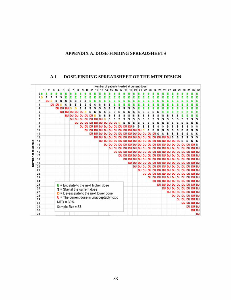
APPENDIX A. DOSE-FINDING SPREADSHEETS
A.1 DOSE-FINDING SPREADSHEET OF THE MTPI DESIGN

34
A.2 DOSE-FINDING SPREADSHEET OF THE BOIN DESIGN
1 2 3 4 5 6 7 8 9 10 11 12 13 14 15 16 17 18 19 20 21 22 23 24 25 26 27 28 29 30 31 32 330 E E E E E E E E E E E E E E E E E E E E E E E E E E E E E E E E E1 D D S S E E E E E E E E E E E E E E E E E E E E E E E E E E E E E2 D D D D S S S E E E E E E E E E E E E E E E E E E E E E E E E E3 DU DU D D D D S S S S E E E E E E E E E E E E E E E E E E E E E4 DU DU DU D D D D D S S S S S E E E E E E E E E E E E E E E E E5 DU DU DU DU DU D D D D S S S S S S S S E E E E E E E E E E E E6 DU DU DU DU DU DU D D D D D S S S S S S S S S E E E E E E E E7 DU DU DU DU DU DU DU D D D D D D S S S S S S S S S S E E E E8 DU DU DU DU DU DU DU DU DU D D D D D D S S S S S S S S S S S9 DU DU DU DU DU DU DU DU DU DU DU D D D D D D S S S S S S S S
10 DU DU DU DU DU DU DU DU DU DU DU DU D D D D D D S S S S S S11 DU DU DU DU DU DU DU DU DU DU DU DU DU DU D D D D D D S S S12 DU DU DU DU DU DU DU DU DU DU DU DU DU DU DU DU D D D D D D13 DU DU DU DU DU DU DU DU DU DU DU DU DU DU DU DU DU D D D D14 DU DU DU DU DU DU DU DU DU DU DU DU DU DU DU DU DU DU DU D15 DU DU DU DU DU DU DU DU DU DU DU DU DU DU DU DU DU DU DU16 DU DU DU DU DU DU DU DU DU DU DU DU DU DU DU DU DU DU17 DU DU DU DU DU DU DU DU DU DU DU DU DU DU DU DU DU18 DU DU DU DU DU DU DU DU DU DU DU DU DU DU DU DU19 DU DU DU DU DU DU DU DU DU DU DU DU DU DU DU20 DU DU DU DU DU DU DU DU DU DU DU DU DU DU21 DU DU DU DU DU DU DU DU DU DU DU DU DU22 DU DU DU DU DU DU DU DU DU DU DU DU23 DU DU DU DU DU DU DU DU DU DU DU24 DU DU DU DU DU DU DU DU DU DU25 DU DU DU DU DU DU DU DU DU26 DU DU DU DU DU DU DU DU27 DU DU DU DU DU DU DU28 DU DU DU DU DU DU29 DU DU DU DU DU30 DU DU DU DU31 DU DU DU32 DU DU33 DU
Number of patients treated at current dose
35
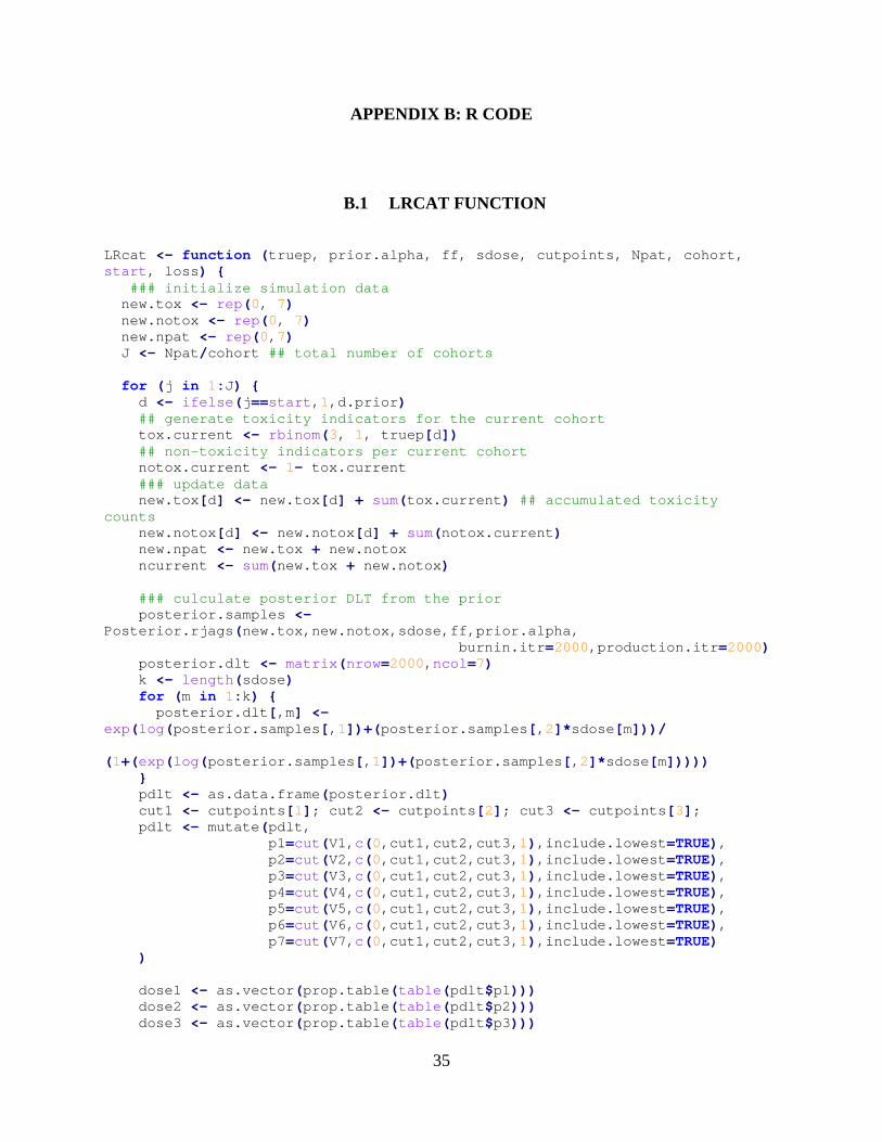
APPENDIX B: R CODE
B.1 LRCAT FUNCTION
LRcat <- function (truep, prior.alpha, ff, sdose, cutpoints, Npat, cohort, start, loss) { ### initialize simulation data new.tox <- rep(0, 7) new.notox <- rep(0, 7) new.npat <- rep(0,7) J <- Npat/cohort ## total number of cohorts for (j in 1:J) {
d <- ifelse(j==start,1,d.prior) ## generate toxicity indicators for the current cohort
tox.current <- rbinom(3, 1, truep[d]) ## non-toxicity indicators per current cohort notox.current <- 1- tox.current ### update data new.tox[d] <- new.tox[d] + sum(tox.current) ## accumulated toxicity counts new.notox[d] <- new.notox[d] + sum(notox.current) new.npat <- new.tox + new.notox ncurrent <- sum(new.tox + new.notox) ### culculate posterior DLT from the prior posterior.samples <- Posterior.rjags(new.tox,new.notox,sdose,ff,prior.alpha, burnin.itr=2000,production.itr=2000) posterior.dlt <- matrix(nrow=2000,ncol=7) k <- length(sdose) for (m in 1:k) { posterior.dlt[,m] <- exp(log(posterior.samples[,1])+(posterior.samples[,2]*sdose[m]))/ (1+(exp(log(posterior.samples[,1])+(posterior.samples[,2]*sdose[m])))) } pdlt <- as.data.frame(posterior.dlt) cut1 <- cutpoints[1]; cut2 <- cutpoints[2]; cut3 <- cutpoints[3]; pdlt <- mutate(pdlt, p1=cut(V1,c(0,cut1,cut2,cut3,1),include.lowest=TRUE), p2=cut(V2,c(0,cut1,cut2,cut3,1),include.lowest=TRUE), p3=cut(V3,c(0,cut1,cut2,cut3,1),include.lowest=TRUE), p4=cut(V4,c(0,cut1,cut2,cut3,1),include.lowest=TRUE), p5=cut(V5,c(0,cut1,cut2,cut3,1),include.lowest=TRUE), p6=cut(V6,c(0,cut1,cut2,cut3,1),include.lowest=TRUE), p7=cut(V7,c(0,cut1,cut2,cut3,1),include.lowest=TRUE) ) dose1 <- as.vector(prop.table(table(pdlt$p1))) dose2 <- as.vector(prop.table(table(pdlt$p2))) dose3 <- as.vector(prop.table(table(pdlt$p3)))

36
dose4 <- as.vector(prop.table(table(pdlt$p4))) dose5 <- as.vector(prop.table(table(pdlt$p5))) dose6 <- as.vector(prop.table(table(pdlt$p6))) dose7 <- as.vector(prop.table(table(pdlt$p7))) ### create a data frame containing posterior probability of DLT by categories pdlt.cat <- rbind(dose1,dose2,dose3,dose4,dose5,dose6,dose7) colnames(pdlt.cat) <- c("under","target","excess","unaccept") ### compute the Bayes risk and overdosing probability bayes.risk <- function(loss,d) { sum(loss*d) } risk <- as.vector(apply(pdlt.cat,1,bayes.risk,loss)) ndose <- seq(1,7,1) pdlt.cat <- cbind(ndose,pdlt.cat,risk) pdlt.cat <- as.data.frame(pdlt.cat) ### select the dose for next level ds <- pdlt.cat d.prior <- ds$ndose[which(ds$risk==min(ds$risk))] ### output the result when all patients are recruited if (j==J) {result <- list(d.prior, new.tox, new.npat)} } return(result) }
B.2 SIMULATION (LRCAT/ LRCAT25)
## function to output operation characteristics oc <- function(mtd,ndlt,npat,target.d,D) { d.mtd <- apply(mtd,2,mean) d.mtd <- d.mtd*100 # percentage of MTD on each level p.tox <- ndlt/npat p.tox.mean <- apply(p.tox,2,mean,na.rm=TRUE) # toxicity probability on each level d.pat <- apply(npat,2,mean) # allocation of patients avg.n <- mean(rowSums(npat)) # average number of total patients avg.dlt <- mean(rowSums(ndlt)) # average number of DLT avg.pct.dlt <- mean(rowSums(ndlt)/rowSums(npat)) # average percentage of dlt overrisk <- if(target.d <= (D-1)) { xx <- vector(mode="numeric", length=nrow(npat)) for (i in 1:nrow(npat)) { xx[i] <- sum(npat[i,(target.d+1):D])/sum(npat[i,]) # percentage of risk of overdosing } (length(xx[which(xx>0.6)])/nrow(npat))*100 } else 0 underrisk <- if(target.d >= 2) {

37
xx <- vector(mode="numeric", length=nrow(npat)) for (i in 1:nrow(npat)) { xx[i] <- sum(npat[i,1:(target.d-1)])/sum(npat[i,]) # percentage of risk of underdosing } (length(xx[which(xx>0.8)])/nrow(npat))*100 } else 0 ocs <- list(d.mtd,p.tox.mean,d.pat,avg.n,avg.dlt,avg.pct.dlt,overrisk,underrisk) ocs <- setNames(ocs, c("PCS","Toxicity probability","Pt. allocation", "Avg. total patient","Avg. DLT","Avg.% of DLT", "Risk of Overdosing","Risk of Underdosing")) return(ocs) } ######################## LRcat25 simulation ######################### LRcat25.sim <- function (truep, nsim) { mtd1 <- matrix(nrow=nsim,ncol=8); mtd1[] <- 0L ndlt1 <- matrix(nrow=nsim,ncol=7) npat1 <- matrix(nrow=nsim,ncol=7) for (i in 1:nsim) { LRcat25<- LRcat25(truep=truep, prior.alpha=list(4, mu3, Sigma3), ff="logit2", sdose=sdose, cutpoints=c(0.2,0.35,0.6), Npat=36, cohort=3, start=1, loss=loss1) if (LRcat25[[1]] > 0) { mtd1[i,(LRcat25[[1]]+1)] <- 1 } else { mtd1[i,1] <- 1 } ndlt1[i,] <- LRcat25[[2]] npat1[i,] <- LRcat25[[3]] } return(list(mtd1,ndlt1,npat1)) } LRcat25.1 <- LRcat25.sim(s1, nsim) lrcat25.1 <- oc(LRcat25.1[[1]],LRcat25.1[[2]],LRcat25.1[[3]],1,7) LRcat25.2 <- LRcat25.sim(s2, nsim) lrcat25.2 <- oc(LRcat25.2[[1]],LRcat25.2[[2]],LRcat25.2[[3]],2,7) LRcat25.3 <- LRcat25.sim(s3, nsim) lrcat25.3 <- oc(LRcat25.3[[1]],LRcat25.3[[2]],LRcat25.3[[3]],2,7) LRcat25.4 <- LRcat25.sim(s4, nsim) lrcat25.4 <- oc(LRcat25.4[[1]],LRcat25.4[[2]],LRcat25.4[[3]],4,7) LRcat25.5 <- LRcat25.sim(s5, nsim) lrcat25.5 <- oc(LRcat25.5[[1]],LRcat25.5[[2]],LRcat25.5[[3]],4,7) LRcat25.6 <- LRcat25.sim(s6, nsim) lrcat25.6 <- oc(LRcat25.6[[1]],LRcat25.6[[2]],LRcat25.6[[3]],6,7) LRcat25.7 <- LRcat25.sim(s7, nsim) lrcat25.7 <- oc(LRcat25.7[[1]],LRcat25.7[[2]],LRcat25.7[[3]],6,7) LRcat25.8 <- LRcat25.sim(s8, nsim) lrcat25.8 <- oc(LRcat25.8[[1]],LRcat25.8[[2]],LRcat25.8[[3]],7,7) ######################## LRcat simulation ######################### LRcat.sim <- function (truep, nsim, D) { mtd2 <- matrix(nrow=nsim,ncol=D+1); mtd2[] <- 0L

38
ndlt2 <- matrix(nrow=nsim,ncol=D) npat2 <- matrix(nrow=nsim,ncol=D) for (i in 1:nsim) { LRcat <- LRcat(truep=truep, prior.alpha=list(4, mu3, Sigma3), ff="logit2", sdose=sdose, cutpoints=c(0.2,0.35,0.6), Npat=36, cohort=3, start=1, loss=loss1) if (LRcat[[1]] > 0) { mtd2[i,(LRcat[[1]]+1)] <- 1 } else { mtd2[i,1] <- 1 } ndlt2[i,] <- LRcat[[2]] npat2[i,] <- LRcat[[3]] } return(list(mtd2,ndlt2,npat2)) } LRcat1 <- LRcat.sim(s1, nsim, 7) lrcat1 <- oc(LRcat1[[1]],LRcat1[[2]],LRcat1[[3]],1,7) LRcat2 <- LRcat.sim(s2, nsim, 7) lrcat2 <- oc(LRcat2[[1]],LRcat2[[2]],LRcat2[[3]],2,7) LRcat3 <- LRcat.sim(s3, nsim, 7) lrcat3 <- oc(LRcat3[[1]],LRcat3[[2]],LRcat3[[3]],2,7) LRcat4 <- LRcat.sim(s4, nsim, 7) lrcat4 <- oc(LRcat4[[1]],LRcat4[[2]],LRcat4[[3]],4,7) LRcat5 <- LRcat.sim(s5, nsim, 7) lrcat5 <- oc(LRcat5[[1]],LRcat5[[2]],LRcat5[[3]],4,7) LRcat6 <- LRcat.sim(s6, nsim, 7) lrcat6 <- oc(LRcat6[[1]],LRcat6[[2]],LRcat6[[3]],6,7) LRcat7 <- LRcat.sim(s7, nsim, 7) lrcat7 <- oc(LRcat7[[1]],LRcat7[[2]],LRcat7[[3]],6,7) LRcat8 <- LRcat.sim(s8, nsim, 7) lrcat8 <- oc(LRcat8[[1]],LRcat8[[2]],LRcat8[[3]],7,7)
B.3 PLOTS FOR SIMULATION RESULTS
############## Percentage of selected MTD on each dose level ############### bar.mtd <- function(truep,target.d,crm,mcrm,mtpi,lrcat25,lrcat,boin) { xaxis <- c('0','1','2','3','4','5','6','7') color <- rep(0,8) color[(target.d+1)] <- 8 par(mfrow = c(1, 6), mar=c(4,2.5,2,1), omi=c(0.2,0.2,0.2,0)) p1 <- barplot(crm[[1]],ylim=c(0,95),main="CRM",names.arg=xaxis,col=color) lines(x=p1[2:8], y=truep*100, type="b", pch=16, lty=1, col=4) p2 <- barplot(mcrm[[1]],ylim=c(0,95),main="mCRM",names.arg=xaxis,col=color) lines(x=p2[2:8], y=truep*100, type="b", pch=16, lty=1, col=4) p3 <- barplot(mtpi[[1]],ylim=c(0,95),main="mTPI",names.arg=xaxis,col=color) lines(x=p3[2:8], y=truep*100, type="b", pch=16, lty=1, col=4) boin.mtd <- c(boin$pctearlystop[1],boin$selpercent) p4 <- barplot(boin.mtd,ylim=c(0,95),main="BOIN",names.arg=xaxis,col=color)

39
lines(x=p4[2:8], y=truep*100, type="b", pch=16, lty=1, col=4) p5 <- barplot(lrcat[[1]],ylim=c(0,95),main="LRcat",names.arg=xaxis,col=color) lines(x=p5[2:8], y=truep*100, type="b", pch=16, lty=1, col=4) p6 <- barplot(lrcat25[[1]],ylim=c(0,95),main="LRcat25",names.arg=xaxis,col=color) lines(x=p6[2:8], y=truep*100, type="b", pch=16, lty=1, col=4) mtext("MTD Selection Percentage", side=2, outer=T, at=0.5) } ## plotting scenarios 1-8 pdf("PCS new.pdf",height=6,width=7) par(mfrow = c(2, 1)) bar.mtd1(s1,1,crm1,mcrm1,mtpi1,lrcat25.1,lrcat1,boin1) mtext("Scenario 1", side=3, outer=T, at=0.5) bar.mtd1(s2,2,crm2,mcrm2,mtpi2,lrcat25.2,lrcat2,boin2) mtext("Scenario 2", side=3, outer=T, at=0.5) bar.mtd1(s3,2,crm3,mcrm3,mtpi3,lrcat25.3,lrcat3,boin3) mtext("Scenario 3", side=3, outer=T, at=0.5) bar.mtd1(s4,4,crm4,mcrm4,mtpi4,lrcat25.4,lrcat4,boin4) mtext("Scenario 4", side=3, outer=T, at=0.5) bar.mtd1(s5,4,crm5,mcrm5,mtpi5,lrcat25.5,lrcat5,boin5) mtext("Scenario 5", side=3, outer=T, at=0.5) bar.mtd1(s6,6,crm6,mcrm6,mtpi6,lrcat25.6,lrcat6,boin6) mtext("Scenario 6", side=3, outer=T, at=0.5) bar.mtd1(s7,6,crm7,mcrm7,mtpi7,lrcat25.7,lrcat7,boin7) mtext("Scenario 7", side=3, outer=T, at=0.5) bar.mtd2(s8,7,crm8,mcrm8,mtpi8,lrcat25.8,lrcat8,boin8) mtext("Scenario 8", side=3, outer=T, at=0.5) dev.off() ###################### Patient allocation ############################# bar.pat1 <- function(target.d,crm,mcrm,mtpi,lrcat25,lrcat,boin) { xaxis <- c('1','2','3','4','5','6','7') color <- rep(0,7) color[target.d] <- 8 par(mfrow = c(1, 6), omi=c(0.2,0.2,0.2,0), par(mar=c(4,2.5,2,1))) p1 <- barplot(crm[[3]],ylim=c(0,25),main="CRM",names.arg=xaxis,col=color) p2 <- barplot(mcrm[[3]],ylim=c(0,25),main="mCRM",names.arg=xaxis,col=color) p3 <- barplot(mtpi[[3]],ylim=c(0,25),main="mTPI",names.arg=xaxis,col=color) p4 <- barplot(boin$nptsdose,ylim=c(0,25),main="BOIN",names.arg=xaxis,col=color) p5 <- barplot(lrcat[[3]],ylim=c(0,25),main="LRcat",names.arg=xaxis,col=color) p6 <- barplot(lrcat25[[3]],ylim=c(0,25),main="LRcat25",names.arg=xaxis,col=color) mtext("Avg. Allocated Patients", side=2, outer=T, at=0.5) } ## plotting scenarios 1-8 bar.pat1(1,crm1,mcrm1,mtpi1,lrcat25.1,lrcat1,boin1)

40
mtext("Scenario 1", side=3, outer=T, at=0.5) bar.pat1(2,crm2,mcrm2,mtpi2,lrcat25.2,lrcat2,boin2) mtext("Scenario 2", side=3, outer=T, at=0.5) bar.pat1(2,crm3,mcrm3,mtpi3,lrcat25.3,lrcat3,boin3) mtext("Scenario 3", side=3, outer=T, at=0.5) bar.pat2(4,crm4,mcrm4,mtpi4,lrcat25.4,lrcat4,boin4) mtext("Scenario 4", side=3, outer=T, at=0.5) bar.pat1(4,crm5,mcrm5,mtpi5,lrcat25.5,lrcat5,boin5) mtext("Scenario 5", side=3, outer=T, at=0.5) bar.pat1(6,crm6,mcrm6,mtpi6,lrcat25.6,lrcat6,boin6) mtext("Scenario 6", side=3, outer=T, at=0.5) bar.pat1(6,crm7,mcrm7,mtpi7,lrcat25.7,lrcat7,boin7) mtext("Scenario 7", side=3, outer=T, at=0.5) bar.pat2(7,crm8,mcrm8,mtpi8,lrcat25.8,lrcat8,boin8) mtext("Scenario 8", side=3, outer=T, at=0.5) ################ Average Percentage of Toxicity####################### bar.tox <- function(crm,mcrm,mtpi,boin,lrcat,lrcat25,title) { crm.tox <- crm[[6]] mcrm.tox <- mcrm[[6]] mtpi.tox <- mtpi[[6]] boin.tox <- (boin$totaltox[1]/boin$totaln[1]) lrcat.tox <- lrcat[[6]] lrcat25.tox <- lrcat25[[6]] tox <- c(crm.tox,mcrm.tox,mtpi.tox,boin.tox,lrcat.tox,lrcat25.tox) barplot(tox, ylim=c(0,0.50), main=title, col=c('#66c2a5','#fc8d62','#8da0cb','#e78ac3','#a6d854','#ffd92f') ) abline(h=0.30,lty=4) #,col="#FFC300" } ## plotting toxicity rate par(mfrow = c(1, 8), family="", oma=c(3,2,1,1), mar=c(3,3,2,1)) bar.tox(crm1,mcrm1,mtpi1,boin1,lrcat1,lrcat25.1,"Scenario 1") bar.tox(crm2,mcrm2,mtpi2,boin2,lrcat2,lrcat25.2,"Scenario 2") bar.tox(crm3,mcrm3,mtpi3,boin3,lrcat3,lrcat25.3,"Scenario 3") bar.tox(crm4,mcrm4,mtpi4,boin4,lrcat4,lrcat25.4,"Scenario 4") bar.tox(crm5,mcrm5,mtpi5,boin5,lrcat5,lrcat25.5,"Scenario 5") bar.tox(crm6,mcrm6,mtpi6,boin6,lrcat6,lrcat25.6,"Scenario 6") bar.tox(crm7,mcrm7,mtpi7,boin7,lrcat7,lrcat25.7,"Scenario 7") bar.tox(crm8,mcrm8,mtpi8,boin8,lrcat8,lrcat25.8,"Scenario 8") mtext("Designs", side=1, outer=T, at=0.5) mtext("Average Toxicity Rate", side=2, outer=T, at=0.5) legend(x=-45,y=-0.10,legend=c('CRM','mCRM','mTPI','BOIN','LRcat','LRcat25'), #col=c('#66c2a5','#fc8d62','#8da0cb','#e78ac3','#a6d854','#ffd92f'), col=c('#000000','#4c4c4c','#7f7f7f','#b2b2b2','#cccccc','#e5e5e5'), #angle=angle1, density=density1, horiz=T, pch=15,bty="0",xpd=NA,cex=1.2,pt.cex=2) dev.off() ######################## Risk of overdosing ######################## bar.over <- function(crm,mcrm,mtpi,boin,lrcat,lrcat25,ylim,title) {

41
#xaxis <- c('3+3','CRM','mTPI','LRcat25','LRcat','BOIN') mtpi.over <- mtpi[[7]] boin.over <- boin$overdose60[1] crm.over <- crm[[7]] mcrm.over <- mcrm[[7]] lrcat.over <- lrcat[[7]] lrcat25.over <- lrcat25[[7]] over <- c(crm.over,mcrm.over,mtpi.over,boin.over,lrcat.over,lrcat25.over) barplot(over, ylim=c(0,ylim), main=title, } ## plotting percentage of overdosing par(mfrow = c(1, 7), family="", oma=c(4,2,1,1), mar=c(2,3,2,1)) bar.over(crm1,mcrm1,mtpi1,boin1,lrcat1,lrcat25.1,35,"Scenario 1") bar.over(crm2,mcrm2,mtpi2,boin2,lrcat2,lrcat25.2,35,"Scenario 2") bar.over(crm3,mcrm3,mtpi3,boin3,lrcat3,lrcat25.3,35,"Scenario 3") bar.over(crm4,mcrm4,mtpi4,boin4,lrcat4,lrcat25.4,35,"Scenario 4") bar.over(crm5,mcrm5,mtpi5,boin5,lrcat5,lrcat25.5,35,"Scenario 5") bar.over(crm6,mcrm6,mtpi6,boin6,lrcat6,lrcat25.6,35,"Scenario 6") bar.over(crm7,mcrm7,mtpi7,boin7,lrcat7,lrcat25.7,35,"Scenario 7") #bar.over(three8,mtpi8,boin8,crm8,lrcat8,lrcat25.8,"Scenario 8") mtext("Designs", side=1, outer=T, at=0.5) mtext("Risk of Overdosing (%)", side=2, outer=T, at=0.5) legend(x=10,y=25,legend=c('CRM','mCRM','mTPI','BOIN','LRcat','LRcat25'), #col=c('#66c2a5','#fc8d62','#8da0cb','#e78ac3','#a6d854','#ffd92f'), col=c('#000000','#4c4c4c','#7f7f7f','#b2b2b2','#cccccc','#e5e5e5'), #angle=angle1, density=density1, horiz=F, pch=15,bty="o",xpd=NA,cex=2,pt.cex=3) dev.off() ####################### Risk of Underdosing ########################## bar.under <- function(crm,mcrm,mtpi,boin,lrcat,lrcat25,ylim,title) { mtpi.under <- mtpi[[8]] boin.under <- boin$underdose80[1] crm.under <- crm[[8]] mcrm.under <- mcrm[[8]] lrcat.under <- lrcat[[8]] lrcat25.under <- lrcat25[[8]] under <- c(crm.under,mcrm.under,mtpi.under,boin.under,lrcat.under,lrcat25.under) barplot(under, ylim=c(0,ylim), main=title, col=c('#000000','#4c4c4c','#7f7f7f','#b2b2b2','#cccccc','#e5e5e5') ) } ## Plot percentage of overdosing par(mfrow = c(1, 7), family="", oma=c(4,2,1,1), mar=c(2,3,2,1)) bar.under(crm2,mcrm2,mtpi2,boin2,lrcat2,lrcat25.2,80,"Scenario 2") bar.under(crm3,mcrm3,mtpi3,boin3,lrcat3,lrcat25.3,80,"Scenario 3") bar.under(crm4,mcrm4,mtpi4,boin4,lrcat4,lrcat25.4,80,"Scenario 4") bar.under(crm5,mcrm5,mtpi5,boin5,lrcat5,lrcat25.5,80,"Scenario 5") bar.under(crm6,mcrm6,mtpi6,boin6,lrcat6,lrcat25.6,80,"Scenario 6") bar.under(crm7,mcrm7,mtpi7,boin7,lrcat7,lrcat25.7,80,"Scenario 7") bar.under(crm8,mcrm8,mtpi8,boin8,lrcat8,lrcat25.8,80,"Scenario 8")

42
mtext("Designs", side=1, outer=T, at=0.5) mtext("Risk of Underdosing (%)", side=2, outer=T, at=0.5) legend(x=10,y=25,legend=c('CRM','mCRM','mTPI','BOIN','LRcat','LRcat25'), col=c('#000000','#4c4c4c','#7f7f7f','#b2b2b2','#cccccc','#e5e5e5'), horiz=F, pch=15,bty="o",xpd=NA,cex=2,pt.cex=3) dev.off()

43
BIBLIOGRAPHY
[1] O. Sverdlov, W. K. Wong and Y. Ryeznik, "Adaptive clinical trial designs for phase I cancer studies," Statistics Surveys, vol. 8, pp. 2-44, 2014.
[2] American Society of Clinical Oncology, "Critical Role of Phase I Clinical Trials in Cancer Treatment," 1996.
[3] B. Storer, "Design and Analysis of Phase I Clinical Trials," Biometrics, no. 45, pp. 925-937, 1989.
[4] A. Ivanova, A. Montazer-Haghighi, S. . G. Mohanty and S. D. Durham, "Improved up-and-down designs for phase I trials," Statistics in Medicine, no. 22, pp. 69-82, 2003.
[5] J. O'Quigley, M. Pepe and L. Fisher, "Continual Reassessment Method: A Practical Design for Phase I Clinical Trials in Cancer," Biometrics, no. 46, pp. 33-48, 1990.
[6] J. Babb, A. Rogatko and S. Zacks, "Cancer phase I clinical trials: efficient dose escalation with overdose control," Statistics in Medicine, no. 17, pp. 1103-1120, 1998.
[7] C. Le Tourneau, J. J. Lee and L. L. Siu, "Dose Escalation Methods in Phase I Cancer Clinical Trials," Journal of the National Cancer Institute, vol. 101, no. 10, pp. 708-720, 20 May 2009.
[8] E. M. J. van Brummelen, A. D. R. Huitema, E. van Werkhoven, J. H. Beijnen and J. H. M. Schellens, "The performance of model-based versus rule-based phase I clinical trials in oncology," Journal of Pharmacokinetics and Pharmacodynamics, no. 43, pp. 235-242, 2016.
[9] Y. Ji, Y. Li and B. N. Bekele, "Dose-finding in phase I clinical trials based on toxicity probability intervals," Clinical Trials, no. 4, p. 235–244, 2007.
[10] Y. Ji, P. Liu, Y. Li and B. N. Bekele, "A modified toxicity probability interval method for dose-finding trials," Clinical Trials, pp. 653-663, 2010.
[11] B. Neuenschwander, M. Branson and T. Gsponer, "Critical aspects of the Bayesian approach to phase I cancer trials," Statistics in Medicine, p. 2420–2439, 2008.
[12] S. Bailey, B. Neuenschwander, G. Laird and M. Branson, "A Bayesian case study in oncology phase I combination dose-finding using logistic regression with covariates," Journal of Biopharmaceutical Statistics, no. 19:3, pp. 469-484, 2009.
[13] S. Liu and Y. Yuan, "Bayesian optimal interval designs for phase I clinical trials," Journal of the Royal Statistica Scociety, pp. 507-523, 2015.
[14] S. M. Lee and Y. K. Cheung, "Model calibration in the continual reassessment method," Clinical Trials, no. 6, pp. 227-238, 2009.
[15] Y. Yuan, K. R. Hess, S. G. Hilsenbeck and M. R. Gilbert, "Bayesian Optimal Interval Design: A Simple and Well-Performing Design for Phase I Oncology Trials," American Association for Cancer Research, pp. 4291-4301, 2016.
[16] G. Laird, "Implementation of Bayesian logistic regression for dose escalation at Novartis Oncology," in Phase I Workshop, New York, 2009.