PROCEEDINGS, 41st Workshop on Geothermal Reservoir Engineering

Stanford University, Stanford, California, February 22-24, 2016

SGP-TR-209

1

Comparison of Nonlinear Formulations for Geothermal Reservoir Simulations

Zhi Yang Wong, Roland Horne and Denis Voskov

Department of Energy Resources Engineering, Stanford University, Stanford, CA 94305

zhiyangw@stanford.edu

Keywords: Nonlinear formulation, geothermal reservoir simulation, convergence

ABSTRACT

This study compared two nonlinear formulations for geothermal reservoir simulation. In particular, it looked at how the nonlinear

formulation of the reservoir simulation equations affects the nonlinear behavior in simulation. Two nonlinear formulations were

investigated: the natural formulation based on a pressure, temperature and saturation (𝑝𝑇𝑆) and the molar formulation based on a

pressure and enthalpy (𝑝ℎ). The main difference between the two formulations is that the natural formulation requires variable

switching and the molar formulation does not. The two different formulations were implemented using Automatic-Differentiation

General Purpose Research Simulator (AD-GPRS). AD-GPRS is a computational framework that allows for fully compositional and

thermal reservoir simulations. This framework was modified to incorporate these two nonlinear formulations. A unified framework

ensures that the differences observed in the nonlinear convergence of simulation are related to the specifics of nonlinear formulation and

not to implementation issues. To verify the results of AD-GPRS simulations, analytical, semianalytical and TOUGH2 solutions were

used to compare the results. Once consistency was verified, a comparison of the nonlinear behavior between the two formulations was

carried out. This was quantified in terms of the time-step size and the number of Newton iterations that each formulation performs. The

results from the numerical experiments showed that the performance of the variable formulations depends on the dominant flow regime.

1. INTRODUCTION

Geothermal reservoir modelling and simulation is an integral part of the management and prediction of geothermal reservoir

performance (O’Sullivan et al., 2001). Reservoir simulations are used to assess the outcomes of different production scenarios

(Axelsson et al., 2003). In order to better represent these geothermal reservoirs there has been an increase in both the demand and

growth in models with complex geometries (O’Sullivan et al. 2013, Burnell et al., 2012), nonlinear physics (O’Sullivan et al., 2013) and

larger models (Yeh et al., 2011).

Due to these added complexities, often a simulator can experience numerical issues when finding a solution to a problem. For instance,

Magnusdottir (2013) experienced difficulty when using a general purpose simulator TOUGH2 (Pruess et al., 1999) to solve a discrete

fracture model. This was thought to be due to the complexity of the numerical grid, resulting in a domain error. Another problem

observed in TOUGH2 was seen by Noy et al. (2012), where a stalling behavior in the time step was observed in a CO2 sequestration

simulation. For geothermal applications, this stalling behavior occurs typically in natural-state geothermal simulations, where large time

steps are taken. Large time steps often challenge reservoir simulations, due to either inaccurate Jacobians or ill-conditioned Jacobians

due to the highly nonlinear nature of the governing equations.

Investigations in the nonlinear and linear solver in a full reservoir simulator can be difficult. Reservoir simulators currently used in the

industry tend to be very complex and difficult to modify. Most existing geothermal modeling tools were developed over 25 years ago

and do not take advantage of modern computational and software architecture advances (Burnell et al., 2015). This makes it difficult to

implement or investigate specific convergence problems or to add additional nonlinear physics to the problem. Even if the problem is

understood and changes are needed to be made, this can also be a difficult task.

In particular, one of the most complicated computations in reservoir simulation is in the construction of the Jacobian used by the

nonlinear solver. The Jacobian matrix contains the derivatives of all the residual equations with respect to each independent variable in

the nonlinear formulation. These residual equations and independent variables can change depending on the type of nonlinear

formulation used or the physics that is modeled. Currently, most codes either employ a manual implementation of the derivatives

(GeoQuest, 2001) or compute a numerical approximation of the derivatives (Pruess et al., 1999). Although a numerical Jacobian would

allow for greater flexibility in the computation, this is less accurate and could result in instabilities when solving the nonlinear equations

(Vanden and Orkwis, 1996). However, a manual implementation would be significantly harder to implement and is tedious when

implementing additional physics or if changes to the formulation is done. These hurdles can make it difficult to implement or investigate

the effects of different formulations or solution strategies for a general purpose simulator.

One method of overcoming this hurdle is to implement an automatic-differentiation library that forms the analytical Jacobian

automatically based on the residual formulation. Automatic-Differentiation General Purpose Research Simulator (AD-GPRS) (Voskov

et al., 2012) is a reservoir modeling platform developed and sustained by the SUPRI-B research group in the Energy Resources

Engineering Department at Stanford University. The nonlinear framework of AD-GPRS is built on the Automatic Differentiation

Expression Templates Library. This library (ADETL) was developed initially by Younis (2011) and further extended by Zhou (2012).

The complete implementation of the geothermal module for AD-GPRS was presented in Wong et al., (2015).

Wong et al.

2

Of the capabilities available in AD-GPRS, the flexible treatment of all nonlinear physics was of most interest to this work. Voskov and

Tchelepi (2012) conducted a comparison between different widely used nonlinear formulations for general-purpose compositional

reservoir simulation. It was found in that study that a natural variable formulation approach performed the best for isothermal

immiscible gas injection process. It was found that for cases where a large number of phase changes occurred, the formulations with the

saturation as the primary variable would provide the best guidance to the nonlinear solver. In the later update (Zaydullin et al., 2013), it

was demonstrated that if gas injection flowed at miscible conditions, the molar formulation performs much better due to the formal

disappearance of two-phase region.

Similar to the study done by Voskov and Tchelepi (2012), this work attempted to compare two main nonlinear formulations for

geothermal reservoir simulation. The two nonlinear formulations applied for geothermal model were the natural variable formulation

with pressure, temperature and saturation used as the primary variables and a persistent variable formulation where pressure and

enthalpy were used as the primary variables. The main focus in this comparison was on the nonlinear challenges due to phase changes in

geothermal simulations. These phase changes present a great difficulty for the nonlinear solver due to the large difference and

discontinuity in thermodynamic parameters between liquid water and steam.

The main difference between these two formulations is that in the pressure-enthalpy formulation the variables remain independent

through phase transitions and are constant both in single-phase and two-phase regions. However for a natural variable approach with

pressure and temperature, a switching in the primary variables is required. Also, the Jacobian and nonlinear convergence for these two

formulations is different due to the differences in primary variables. A pressure-enthalpy approach has been implemented in multiphase

simulators in the past (Pritchett, 1975; Faust and Mercer, 1979; Pruess et al., 1979). One of the drawbacks of these approaches is that

thermodynamic properties are often formulated in terms of the natural variables (temperature and saturation) and calculation in terms of

persistent variables (enthalpy) requires iterative methods (Pruess et al., 1999). However, natural formulation requires a switching of

primary variables between different single- and two-phase conditions. This study aimed to look at these two formulations and to

examine and understand how the choice of the primary variables affect the nonlinear convergence.

2. NUMERICAL FORMULATION

2.1 Governing Equations

For this study, only the transport pure water in two-phase flow was considered. The mass and energy conservation equations for this

problem are:

𝜕

𝜕𝑡(𝜙(𝜌𝑤𝑆𝑤 + 𝜌𝑠𝑆𝑠)) − ∇. (𝜌𝑤𝑢𝑤 + 𝜌𝑠𝑢𝑠) − 𝑄𝑀 = 0 (1)

and

𝜕

𝜕𝑡((1 − 𝜙)𝜌𝑅𝑈𝑅 + 𝜙(𝜌𝑤𝑈𝑤𝑆𝑤 + 𝜌𝑠𝑈𝑠𝑆𝑠))

− ∇. (𝜌𝑤ℎ𝑠𝑢𝑤 + 𝜌𝑠ℎ𝑠𝑢𝑠) − ∇. (𝐾∇𝑇) − 𝑄𝐸

= 0

(2)

Where:

𝜙 is the porosity of the rock

𝜌𝑘 is the mass density of phase 𝑘

𝑆𝑘 is the saturation of phase 𝑘

𝑢𝑘 is the velocity of phase 𝑘

𝑄 is the source/sink term

ℎ𝑘 is the enthalpy of phase 𝑘

𝑈𝑘 is the internal energy of phase 𝑘

𝐾 is the total conductivity of the fluid and rock

Here the subscripts 𝑤/𝑠 represents the two phases water and steam, and the subscript 𝑅 represents the rock. Both 𝜌𝑘 , ℎ𝑘 in each phase

depend on the phase state of the fluid. At single-phase conditions, 𝜌𝑘 and ℎ𝑘 are both functions of pressure and temperature. However,

at two-phase conditions, 𝜌𝑘 and ℎ𝑘 will only depend on pressure since now pressure and temperature are dependent on each other

(𝑝 = 𝑝𝑠𝑎𝑡(𝑇)).

In addition to these two conservation equations, the saturation constraint must be satisfied, the sum of all the phase saturations is 1.

𝑆𝑤 + 𝑆𝑠 = 1 (3)

Wong et al.

3

2.2 Darcy’s Law

To model the velocity of each phase, Darcy’s law was used to describe the flow through the porous media:

𝑢𝑘 =𝑘𝑘𝑟𝑘

𝜇𝑘∇(𝑝𝑘 + 𝜌𝑘𝑔𝑧) (4)

Where:

𝑢𝑘 is the superficial velocity of phase 𝑘

𝑘 is the rock permeability

𝑘𝑟𝑘 is the relative permeability of phase 𝑘

𝜇𝑘 is the viscosity of phase 𝑘

𝑝𝑘 is the pressure of phase 𝑘

𝑔 is the gravitational constant

𝑧 is the direction of the gravity

𝑘 represents either the water phase or steam phase

2.3 Solution procedure

The finite volume space discretization with a fully implicit method for time approximation was applied to the mass and energy

conservation equations (Equations 1 and 2). The two-point flux approximation (TPFA) method was used to discretize the spatial

dimension for all the numerical solutions in this study. The current implementation of AD-GPRS is capable of a multipoint flux

approximation. This is important in geothermal applications where it is important to accurately represent the complex geology or

fractures. The TPFA implemented in this study is a phase-based, single-point upstream weighted scheme (Aziz and Settari, 1979).

The Newton-Raphson method was used to linearize the system of nonlinear equations into a system of linear equations. This required a

Jacobian matrix to be computed and solved at each nonlinear iteration. The Jacobian matrix contains the derivatives of each nonlinear

equation with respect to nonlinear unknowns. To reduce the size of the entire global linear system, a Schur-complement is applied to the

entire full Jacobian block-wise such that the mass and energy conservation equations are expressed as a function of primary variables

only. The general Schur-complement strategy is described in Cao (2002). This reduction is done on the full Jacobian of each block in

the reservoir. With the reduced Jacobian, the linear system of equations is solved by specified linear solver.

Once the primary variables have been determined, all the secondary variables can be back-calculated using the secondary equations that

are locally defined for each block. Checks are implemented on the solution to ensure that each parameter remains within the physical

range. This involves testing that the pressures, temperatures and enthalpy are positive and stay within the physical region defined by the

thermodynamic relationships.

An integral aspect of a nonlinear solver is the time step selection scheme. This involves a balance between choosing a time step that is

small enough such that the nonlinear solver would still converge but large enough such that the simulation would not take too many

time steps. If the nonlinear solver does not converge, the time step is restarted with a smaller time step. Thus large time steps are

desirable as they would reduce the computational time because there would be less nonlinear and linear solutions to reach a specified

simulation time.

2.4 Primary Variables

A fundamental step in the formulation of the numerical solution for reservoir simulation is the choice of primary variables that are

solved at each linear step. The choice of the primary variables will significantly affect the Jacobian and the derivatives calculated with

respect to each variable. This would affect the nonlinear convergence paths and also impact the size of time steps that the nonlinear

solver converges for.

Although the choice of primary variables is non-unique, the chosen primary variables have to fully define the thermodynamic state of a

block. This would allow the secondary variables to be back-calculated. From Gibb’s phase rule we know that the number of degrees of

freedom to fully define all the thermodynamic variables is:

𝑓 = 𝑁𝑐 + 2 − 𝑁𝑝 (5)

where:

𝑁𝑐 is the number of components

𝑁𝑝 is the number of phases

𝑓 is the number of degrees of freedom to define the intensive thermodynamic variables

There are also 𝑁𝑝 − 1 saturation degrees of freedom that has to be satisfied. Thus the total number of degrees of freedom is:

𝑁𝑓 = (𝑁𝑐 + 2 − 𝑁𝑝) + (𝑁𝑝 − 1) = 𝑁𝑐 + 1 (6)

Wong et al.

4

For the geothermal problem of single-component (water) and a two phase system (liquid water and steam), two primary variables are

required to be solved for each block in the system. This is equal to the number of mass balance equations (𝑁𝑐 = 1) and the number of

energy balance equations (1) per block. There are a number of different combinations that could be chosen as the primary variables for

these simulations.

This study we compare two primary variable formulations: a natural (𝑝𝑇𝑆) formulation and a persistent (𝑝ℎ) formulation. One of the

main differences between these two formulations is that in the persistent formulation, pressure and enthalpy defines the thermodynamic

state for both single- and two-phase conditions. However in the natural formulation, a variable switching is required when transitioning

from single and two-phase conditions. This happened because pressure and temperature become dependent at saturated conditions and

the saturation is used to replace temperature as the primary variable. One implementation benefit of using the natural formulation is that

the most of relationships in governing equations are formulated in terms of pressure, temperature and saturation.

2.5 Pressure-Temperature-Saturation (𝒑𝑻𝑺) Formulation

Table 1: pTS Formulation status table for liquid water and steam

Phases Primary Variables

Status Liquid Water Steam 𝑝 𝑇 𝑆𝑠

0 x - x x -

1 - x x x -

2 x x x (x) x

The 𝑝𝑇𝑆 formulation follows the idea of natural variable formulation developed by (Coats 1980). For the 𝑝𝑇𝑆 formulation, pressure,

temperature and the steam saturation are chosen as primary variables. This choice is dependent on the status of a block. For a pure water

two-phase system, there are only three possible statuses: pure compressed liquid water, superheated steam and a saturated two-phase

system. In single-phase conditions (compressed liquid water and steam), pressure (𝑝) and temperature (𝑇) are the primary variables.

However in two-phase conditions, pressure and temperature are not independent and now are related by 𝑝 = 𝑝𝑠𝑎𝑡(𝑇). The steam

saturation is used to replace 𝑇 as a primary variable in the two-phase region. A summary of this schema is shown in Table 1.

2.5.1 Phase Change Algorithm

Based on the current status of a block, the logic for determining the new status of a block after each Newton update is shown in

Algorithm 1. It can be seen that through each phase transition, the temperature is preserved from the updated pressure rather than the

pressure from the previous iteration. This was selected because in most flow problems, the temperature changes slower than pressure.

To indicate whether a block has changed phases, the pressure is compared with the saturation pressure. If from this check it indicates

that it is now at two-phase conditions. The primary variables are then switched to pressure and saturation and 𝑆𝑠 = 𝜖 if it was in the

liquid region and 𝑆𝑤 = 𝜖 if it was in the steam region. This 𝜖 was chosen to be 10−4, however it has been observed in Hernandez et al.

(2015) that this value can affect the nonlinear convergence.

Wong et al.

5

2.6 Pressure-Enthalpy (𝒑𝒉) Formulation

The 𝑝ℎ formulation presented here follows the study done by Faust and Mercer (1979). This formulation involves pressure and enthalpy

as the primary variables for all statuses. In this formulation, the primary variables remains unchanged for all statuses. The status of a

block here refers to the same definition as defined in the 𝑝𝑇𝑆 formulation.

2.6.1 Phase Change Algorithm

In single-phase, the enthalpy (ℎ) represents the single-phase fluid enthalpy. In two-phase regions, ℎ represents the enthalpy of the two-

phase fluid mixture defined as:

ℎ =𝑆𝑤𝜌𝑤ℎ𝑤 + 𝑆𝑠𝜌𝑠ℎ𝑠

𝜌 (7)

Where:

𝑆𝑤/𝑠 is the saturation of water/steam

𝜌𝑤/𝑠 is the saturated density of water/steam

ℎ𝑤/𝑠 is the saturated enthalpy of water/steam

The density of the two phase mixture 𝜌 is defined as:

𝜌 = 𝑆𝑤𝜌𝑤 + 𝑆𝑠𝜌𝑠 (8)

Also, from the saturation constraint (Equation 3) we can rearrange to obtain an equation for 𝑆𝑠

𝑆𝑠 =𝜌𝑤(ℎ𝑤 − ℎ)

ℎ(𝜌𝑠 − 𝜌𝑤) − (ℎ𝑠𝜌𝑠 − ℎ𝑤𝜌𝑤) (9)

To account for the phase change between statuses, the enthalpy value was compared with the saturated enthalpies for water and steam

respectively. The phase change logic is based upon Equation 9, the algorithm used is shown in Algorithm 2. One of the main differences

in this phase change algorithm in comparison to the 𝑝𝑇𝑆 formulation, is that when transitioning to the two-phase region, the saturation

could be calculated based on the pressure and enthalpy update. Thus there does not need to be an 𝜖 value introduced. It is not obvious

whether this approach would be better when blocks change phases, as this could result in oscillatory solutions when transitioning across

the phase boundary, since the derivative on either side of the phase boundary would be significantly different.

3. IMPLEMENTATION

3.1 AD-GPRS

The implementation and investigations for this study were completed using AD-GPRS. AD-GPRS was designed to be a flexible

reservoir research simulator that focuses on an extendable code structure. This flexibility provides to capability of investigating different

physics and numerical formulation with ease. Consequently, a modular object-oriented code structure was implemented. This flexible

framework was crucial when implementing the two above formulations. This both allows for minimal code duplication but also

provides a consistent framework for the comparison between the 𝑝𝑇𝑆 and 𝑝ℎ formulation.

Wong et al.

6

AD-GPRS solves the governing mass and energy balance equations, by discretizing with the finite volume method and linearizing the

nonlinear equations using a Newton-Raphson based method. The nonlinear framework of AD-GPRS was built on the Automatic

Differentiation Expression Template library developed at Stanford University (Younis 2011, Zhou 2012). A description of the 𝑝𝑇𝑆

implementation and further details of the geothermal AD-GPRS is described in Wong et al. (2015).

3.2 Consistency check

To verify the simulation results obtained from AD-GPRS, a code comparison study was completed based on the results from the 1980

Code Comparison completed at Stanford (Stanford Geothermal Program 1980). The results of both formulations were tested for

consistency using these different test cases. These test cases involved testing the obtained results against analytical, semi-analytical and

TOUGH2 results. A full description and discussion of the results for the numerical results and reference solutions can be seen in Wong

(2015)

3.2.1 Injection

This test case (Test Case 1) involves a one-dimensional, radial steady-state flow with unsteady heat transport for single-phase liquid

water. The objective of this test case is to verify the heat conduction and convection of single-phase liquid water.

Figure 1 shows the spatial temperature distribution at the final time of 109 seconds and the temporal temperature distribution at each

time step for the block with its center at 37.5 m. Figure 1 a and b shows the same results as Figure 1 c and d and with the published

results obtained in the 1980 Stanford Code Comparison study. As it can be seen from the results, AD-GPRS reproduce the analytical

solution quite accurately. The temperature distribution over time for the block at 37.5 m is slightly greater than the analytical Advonin

solution. This deviation can be observed by several results in the Code Comparison Study except for the one code that managed to

match the results completely. It is important to note that in this code, they implemented a central-difference scheme rather than the

traditional upwinding scheme. This suggests that the deviation between the two results could be from the error of approximation, since a

central-difference has a second order of approximation, while the upwinding scheme is first order. However an upwinding scheme is

used to guarantee that the entropy solution is reached for hyperbolic transport.

Figure 1: Temperature distribution (a) at time = 109 seconds (Left) and the temperature distribution corresponding to the block

with a block center of 37.5 (b) over the simulated time period, Results from Code Comparison study can be seen on the right (c

and d)

3.2.2 Production

This simulation involved the propagation of a flash front moving outwards radially from the production well. To verify the results

obtained by AD-GPRS, a similarity semi-analytical result was used from O’Sullivan (1981). Initially, the reservoir begins completely

filled with liquid water, approximately 5 bars above the saturation pressure for water at a temperature of 573.15K. This boiling occurs

approximately 10 m from the well after about 1 day. Numerically, this problem is more difficult than the previous case due to this phase

change behavior. In Figure 2, it can be seen that this match is not as close as in the previous cases. The same numerical dispersion was

also observed in the smearing of the shock front as seen in the saturation plot. There is also a deviation in the pressure results at the

point where the solution goes to two-phase. This same deviation was also observed in the 1980 Code Comparison Study (Figure 2)

Wong et al.

7

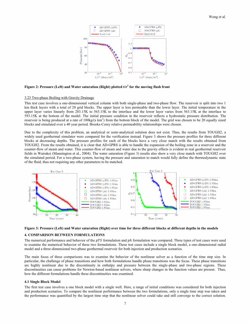
Figure 2: Pressure (Left) and Water saturation (Right) plotted t/r2 for the moving flash front

3.23 Two-phase Boiling with Gravity Drainage

This test case involves a one-dimensional vertical column with both single-phase and two-phase flow. The reservoir is split into two 1

km thick layers with a total of 20 grid blocks. The upper layer is less permeable than the lower layer. The initial temperature in the

upper layer varies linearly from 283.15K to 563.15K to the interface and the lower layer varies from 563.15K at the interface to

593.15K at the bottom of the model. The initial pressure condition in the reservoir reflects a hydrostatic pressure distribution. The

reservoir is being produced at a rate of 100kg/(s km2) from the bottom block of the model. The grid was chosen to be 20 equally sized

blocks and simulated over a 40 year period. Brooks-Corey relative permeability relationships were chosen.

Due to the complexity of this problem, an analytical or semi-analytical solution does not exist. Thus, the results from TOUGH2, a

widely used geothermal simulator were compared for the verification instead. Figure 3 shows the pressure profiles for three different

blocks at decreasing depths. The pressure profiles for each of the blocks have a very close match with the results obtained from

TOUGH2. From the results obtained, it is clear that AD-GPRS is able to handle the expansion of the boiling zone in a reservoir and the

counter-flow of steam and water. This counter-flow of steam and water due to the gravity effects is evident in real geothermal reservoir

fields in Wairakei (Mannington et al., 2004). The water saturation (Figure 3) results also show a very close match with TOUGH2 over

the simulated period. For a two-phase system, having the pressure and saturation to match would fully define the thermodynamic state

of the fluid, thus not requiring any other parameters to be matched.

Figure 3: Pressure (Left) and Water saturation (Right) over time for three different blocks at different depths in the models

4. COMPARISON BETWEEN FORMULATIONS

The numerical performance and behavior of the 𝑝𝑇𝑆 formulation and 𝑝ℎ formulation was compared. Three types of test cases were used

to examine the numerical behavior of these two formulations. These test cases include a single block model, a one-dimensional radial

model and a three-dimensional two-phase geothermal reservoir for both injection and production scenarios.

The main focus of these comparisons was to examine the behavior of the nonlinear solver as a function of the time step size. In

particular, the challenge of phase transitions and how both formulations handle phase transitions was the focus. These phase transitions

are highly nonlinear due to the discontinuity in enthalpy and pressure between the single-phase and two-phase regions. These

discontinuities can cause problems for Newton-based nonlinear solvers, where sharp changes in the function values are present. Thus,

how the different formulations handle these discontinuities was examined.

4.1 Single Block Model

The first test case involves a one block model with a single well. Here, a range of initial conditions was considered for both injection

and production scenarios. To compare the nonlinear performance between the two formulations, only a single time step was taken and

the performance was quantified by the largest time step that the nonlinear solver could take and still converge to the correct solution.

Wong et al.

8

These time steps were calculated by iteratively checking whether a time step converges. The time step recorded is the largest time step

at which the nonlinear solver converges. The discrete time step increment was limited by 0.5 days, so for the Δ𝑡 reported, the next time

step of Δ𝑡+ 0.5, will lead to non-convergent behavior of the nonlinear solver.

The model contained only a single block, with pore volume of 3200m3 and an initial temperature of 568.3K. This temperature was

selected to reflect the high temperature of conventional geothermal reservoirs. A range of different initial conditions for the block was

considered. A summary of the initial conditions for each of the different cases can be seen in Table 2. (Note: the saturation pressure at a

temperature of 568.3K is 80 bar). These initial conditions were chosen to reflect the different typical block conditions that are expected

to exist in a geothermal reservoir. These range from liquid water, a two-phase region and a superheated steam region. For the two-phase

region, three different saturation cases were tested, a high steam saturation case, high water saturation case and a case with 0.5 water

saturation.

Table 2: Initial conditions for the different single block models

Initial Conditions

Case 𝒑 [bar] 𝑻 [K] 𝑺𝒔

A 60 568.3 1.0

B 75 568.3 1.0

C 80 568.3 0.99

D 80 568.3 0.5

E 80 568.3 0.01

F 85 568.3 0.0

G 100 568.3 0.0

Here we use a GMRES linear solver with the BILU preconditioner with a fill-in of 0. The linear solver tolerance was set to 10-10 for 20

maximum iterations. The nonlinear solver was chosen to have a tight tolerance of 10-12 and the maximum linear iterations was set to be

??. The relative permeability curves chosen to be X-Curves with zero residual water and steam saturations. A sufficiently large well

index of 105 was chosen such that the well constraint would not affect the nonlinear convergence.

4.1.1 Production

The production performed by a single well that was producing 1kg/sec of fluid, the mass of water both in the liquid and gas phase. The

initial conditions that were considered are shown in Table 2.

The maximum time step was compared for the two formulations for a production scenario. We will compare the time step size in terms

of a CFL number, for the single block case it is defined as:

𝐶𝐹𝐿𝑚𝑎𝑥 =Δ𝑡𝑄

𝑃𝑉 (9)

Where:

Δ𝑡 is the maximum time step

𝑄 is the volume injection rate

𝑃𝑉 is the pore volume of the block

For Cases 𝐴, 𝐵, 𝐶 the time step size was limited by the amount of mass in the block rather than the nonlinear solver. This means that if

the solution would not converge it would be because the well would be drawing all the fluid out of the block, resulting in an unphysical

solution.

For the conditions that started at liquid water (Cases F, G), both the 𝑝𝑇𝑆 formulation and 𝑝ℎ formulation struggled at crossing this phase

transition and only a small time step was able to be taken. For these scenarios, the solutions converged to a solution with only a small

(𝑆𝑠 = 0.05) steam saturation. This was because in the single-phase liquid region, if the time step taken was too large, the pressure

would drop too low and reach a negative pressure. This results in the time step being limited by the pressure dropping to zero in the first

Newton iteration. For the production case, we observed that the 𝑝𝑇𝑆 and 𝑝ℎ formulation performed equally well for e cases, both in

terms of the size of the time step and the number of Newton iterations.

Wong et al.

9

Table 3: Maximum time step, CFL, Newton iterations and the solution after the corresponding time step for the two

formulations when producing from a single block (The superscript 𝒏 + 𝟏 on 𝒑, 𝑺𝒔 represents the pressure and steam saturation

after one time step size 𝚫𝒕)

𝒑𝑻𝑺 Formulation 𝒑𝒉 Formulation

Case 𝚫𝒕 [days] CFL [-] 𝒑𝒏+𝟏 [bar] 𝑺𝒔𝒏+𝟏[-]

Newton

Iterations 𝚫𝒕 [days] CFL [-] 𝒑𝒏+𝟏 [bar] 𝑺𝒔

𝒏+𝟏[-] Newton

Iterations

A-C ∞ ∞ * * * ∞ ∞ * * *

D 14.5 0.606 39 0.993 9 14.5 0.606 39 0.9934 9

E 26 1.087 15.3 0.947 9 27.5 1.149 4.8 0.9885 6

F 1.5 0.063 79.3 0.054 4 0.1 0.165 79.8 10-4 3

G 1.5 0.063 78.6 0.042 4 0.4 0.368 79.0 10-4 3

4.1.2 Injection

The injection well was set to be into a single well that was injecting 433.15K water at 1kg/sec. Similar to the production case, the same

range of initial conditions were considered (Table 4).

The maximum time step for the different initial conditions for the injection of cold water was analyzed. In Table 4 the different

maximum time steps (Δ𝑡) for the different initial conditions is shown. Again, the CFL number was computed using Equation 9

however rather than 𝑄 being the produced fluid, 𝑄 was the injected fluid instead.

Table 4: Maximum time step, CFL, Newton iterations and the solution after the corresponding time step for the two

formulations when injecting cold water into a single block (The superscript 𝒏 + 𝟏 on 𝒑, 𝑺𝒔 represents the pressure and steam

saturation after one time step size 𝚫𝒕)

𝒑𝑻𝑺 Formulation 𝒑𝒉 Formulation

Case 𝚫𝒕 [days] CFL [-] 𝒑𝒏+𝟏 [bar] 𝑺𝒔𝒏+𝟏[-]

Newton

Iterations 𝚫𝒕 [days] CFL [-] 𝒑𝒏+𝟏 [bar] 𝑺𝒔

𝒏+𝟏[-] Newton

Iterations

A 3.5 0.059 71 0.9206 4 3 0.059 68.4 0.882 5

B 3.5 0.606 39 0.993 9 3 0.606 71.08 0.887 7

C 25.5 1.087 15.3 0.947 9 1.5 1.149 75.63 0.930 9

D-G ∞ * * * * ∞ * * * *

A maximum Δ𝑡 of ∞ meant that a large enough time step was specified such that fluid could be injected into a block until the point

where the pressure becomes unphysical and lies outside of the applicable for the range of the thermodynamic relationships. Thus for

these cases (Cases D-G) we did not report the time step taken or the time result after that given time step, because the time step is

effectively only bounded by the physical limits. For the cases that did have a limit on the time step size, all the cases were not

converging due to a Newton iteration converging to a nonphysical solution. This meant that either 𝑝, 𝑇 or ℎ were outside of the physical

or thermodynamic range. This is due to the inaccuracy of the linearization of the nonlinear residual equation in the Newton's Method.

Comparing the 𝑝𝑇𝑆 and 𝑝ℎ Formulation, all the initial condition scenarios examined had similar time step sizes and results, except for

cases where the initial conditions of the block are within the two-phase region with a high gas saturation (C(𝑆𝑠 = 0.99) and D(𝑆𝑠 =0.5)). For an initial condition of 𝑆𝑠 = 0.99, the 𝑝𝑇𝑆 formulation was able to take a time step 15 times larger time step in comparison to

the 𝑝ℎ formulation.

As expected, the cases where the initial block condition was either fully saturated or had a high steam saturation, both formulations

struggled to converge at a large time step. It is important to note that the 𝑝𝑇𝑆 formulation converges in half the number of Newton

iterations. For the cases where the solution started as superheated steam, both the 𝑝𝑇𝑆 and the 𝑝ℎ formulations were only able to

converge to a solution at around 𝑆𝑠 ≈ 0.9. The time steps that did not converge, were solutions that converged to negative pressures that

caused the thermodynamic formulations to fail and not continue. This reflects the predicted ``negative compressibility'' behavior

described by Coats (1980), where the pressure would drop while injecting mass. This nonlinear behavior would often cause the

nonlinear solution to converge to a negative pressure or enthalpy value.

Wong et al.

10

4.2 One-dimensional Radial model

This comparison model was identical to the reservoir model used in the consistency study. However for this case a more aggressive time

stepping scheme was implemented to compare the number of time step cuts between the two formulations. The total simulation time

was set to 105 days. The initial time step was set to 10−5 days with an increment multiplier of 10 and a maximum time step of 104

days. The linear solver GMRES with the BILU preconditioner with a fill-in of 0. The linear solver tolerance was set to 10−10 and the

maximum iterations was set to 20. The nonlinear solver had a tolerance of 10−6 and the maximum nonlinear iterations was 20.

4.2.1 Comparison

The objective of this reservoir model was to compare how the two different formulations handle a simple one-dimensional flow problem

that is mostly governed by the flow aspect of the problem. In both cases there is a moving phase change front either from water to steam

or vice versa. It was found that the 𝑝𝑇𝑆 formulation performed better for both the production and injection scenarios (see Table 5). This

is hypothesized to be due to the inclusion of saturation as a primary variable and the hyperbolic nature of the saturation equation.

However, it is important to note that both formulations performed relatively well, considering the aggressive time stepping scheme that

was used.

Table 5: Comparison between pTS and ph formulations for one-dimensional production scenario

Production Scenario Injection Scenario

𝒑𝑻𝑺 Formulation 𝒑𝒉 Formulation 𝒑𝑻𝑺 Formulation 𝒑𝒉 Formulation

Number Time Steps 49 82 43 76

Total Newton Iterations 336 575 341 526

Total Linear Solver Iterations 672 1148 682 1050

Wasted Time Steps 11 45 7 42

Wasted Newton Iterations 114 142 57 156

Wasted Linear Solver Iterations 216 284 101 312

CPU time [seconds] 4.27 6.01 3.27 6.11

4.3 Two-dimensional heterogeneous model

The distribution of permeability and porosity were taken from the top layer of the SPE10 model, the permeability distribution can be

seen in Figure 4 (Christie and Blunt, 2001). There are 60 × 220 × 1 grid blocks, each grid block is 20 × 10 × 70m. Uniform pressure

(40 bar), temperature (523.15K) and water saturation (0.5) was imposed as the initial conditions. The same Brooks-Corey defined in

Case 2 was used for the relative permeability. There were four wells in this model, two injection (𝑞(𝑡) = 𝑞𝑖𝑛𝑗 , 𝑇 = 433.15𝐾) and two

production wells (𝑞(𝑡) = 𝑞𝑝𝑟𝑜𝑑). The well schedule was split into two periods:

0 < 𝑡 ≤ 730 days 𝑞𝑝𝑟𝑜𝑑 = 1728𝑘𝑔/𝑑𝑎𝑦 , 𝑞𝑖𝑛𝑗 = 3456𝑘𝑔/𝑑𝑎𝑦

730 < 𝑡 ≤ 1330 days 𝑞𝑝𝑟𝑜𝑑 = 3456/𝑑𝑎𝑦 , 𝑞𝑖𝑛𝑗 = 6912 𝑘𝑔/𝑑𝑎𝑦

The simulation time was 600 days. The linear solver used was GMRES with the CPR preconditioner with a fill-in of 0. The linear solver

tolerance was set to 10-4 for 100 maximum iterations. The nonlinear solver was chosen to have a tolerance of 10-5 and the maximum

nonlinear iterations was set to be 15.

Figure 4: Log of permeability distribution for the top layer of the SPE 10 model (Black dots represent the two producers, white

dots represents the injectors)

Wong et al.

11

4.3.1 Comparison

The final solution is shown in Figure 5. Both formulations struggled with this reservoir simulation, they both wasted approximately the

same number of time steps completed. The 𝑝𝑇𝑆 formulation required about three times more nonlinear solutions than the 𝑝ℎ

formulation. This is also reflected in the longer CPU time and more linear solutions required by the 𝑝𝑇𝑆 formulation in comparison to

the 𝑝ℎ formulation. This was because the maximum time step that the 𝑝ℎ formulation was converging at was three times larger than the

𝑝𝑇𝑆 formulation (MaxCFL averaged by timesteps), thus requiring three times less time steps. Most of the non-convergent iterations for

both the 𝑝𝑇𝑆 and 𝑝ℎ formulations were due to phase changes. This difference in performance could be explained by the fact that the 𝑝ℎ

formulation predicts an exact value of saturation after the phase switch pTS formulation is using an 𝜖 value as the initial guess for

saturation.

Figure 5: Pressure (Top), Temperature (Middle) and Saturation (Bottom) at end of simulation

Table 6: Comparison between pTS and ph formulations for two-dimensional heterogeneous model

𝒑𝑻𝑺 Formulation 𝒑𝒉 Formulation

Number Time Steps 497 130

Total Newton Iterations 1774 601

Total Linear Solver Iterations 12100 4605

Wasted Time Steps 469 103

Wasted Newton Iterations 6423 1160

Wasted Linear Solver Iterations 40637 9932

MaxCFL averaged by timesteps 0.409 1.578

CPU time [seconds] 6189.9 2327.4

4.4 Three-Dimensional Model

The last is a three-dimensional model based on a reservoir model from the 1980 Code Comparison Study (Stanford Geothermal

Program, 1980). The reservoir model consists of single-phase liquid water with a two-phase zone of immobile steam sandwiched

between a hot and cold water region. Production is performed from a well that is completed below the two-phase zone. The parameters

were chosen such that the boiling in the well occurs after a certain period of production. Although the parameters are relatively

homogeneous, it was used as a prototype for field-wide reservoir development studies. This problem has both three-dimensional flow

Wong et al.

12

with phase transitions and two-phase flow, including gravity drainage. A full discussion on the problem description can be found in

Stanford Geothermal Program (1980).

Figure 6: Schematic of the three-dimensional reservoir model

One of the main changes in the original implementation of the problem is that a finer grid was used in comparison to the code

comparison study. The computational grid had 40 × 50 × 30 total blocks that were 100 × 100 × 60 𝑚 in size. The production well

was completed in the corner block and perforates layers 16-20. The water rate at 1000kg/day was used as the well control.

The simulation time was 600 days. We use the GMRES linear solver with the CPR preconditioner with a fill-in of 0. The linear solver

tolerance was set to 10-5 for 100 maximum iterations. The nonlinear solver was chosen to have a tolerance of 10-4 and the maximum

nonlinear iterations was set to be 10. The time step multiplier was set to 2. To ensure a fair test between both formulations, the same

nonlinear and linear solver settings were used for both formulations.

4.4.1 Comparison

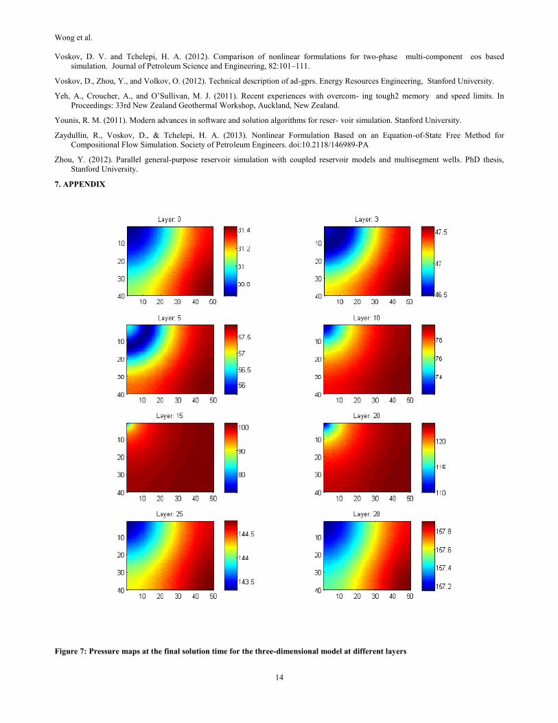
The pressure, temperature and saturation distributions at the final simulation time can be seen in the Appendix (Figure 7, 8 and 9). From

Table 7, it can be seen that the 𝑝ℎ formulation performed better than the 𝑝𝑇𝑆 formulation. It is important to note that the 𝑝ℎ formulation

did not have any wasted time steps for the time stepping scheme used. This means that it is possible for the 𝑝ℎ formulation to have

taken a more aggressive time stepping scheme and to have converged in even less time steps. Again, we observe for this model that the

𝑝ℎ formulation performs better than the 𝑝𝑇𝑆 formulation. This again could be attributed to the large number of phase changes in the

problem and how the 𝑝ℎ formulation is capable of computing an updated saturation when crossing a phase boundary.

Table 7: Comparison between pTS and ph formulations for three-dimensional model

𝒑𝑻𝑺 Formulation 𝒑𝒉 Formulation

Number Time Steps 29 22

Total Newton Iterations 76 49

Total Linear Solver Iterations 327 230

Wasted Time Steps 7 0

Wasted Newton Iterations 58 0

Wasted Linear Solver Iterations 271 0

MaxCFL averaged by timesteps 3.931 5.181

CPU time [seconds] 379.9 152.4

5. DISCUSSION AND CONCLUSIONS

Using a consistent simulation framework, we investigated the nonlinear performance of a 𝑝𝑇𝑆 and 𝑝ℎ formulation for geothermal

reservoir simulation. Specifically we looked at varying degrees of complexity to characterize the performance of both formulations on

different flow regimes. The numerical results of this study indicate that neither the 𝑝𝑇𝑆 or 𝑝ℎ formulation can be definitely choosen as

Wong et al.

13

a preferred approach for geothermal reservoir simulation. Our results show the dependency of nonlinear behavior on the specific

simulation model. From the single block and one-dimensional models it was shown that the 𝑝𝑇𝑆 formulation was able to converge at

larger time steps than the 𝑝ℎ formulation. However, for more complex reservoir models with complex phase transitions and

heterogeneities, the 𝑝ℎ formulation performed better. This could be the difference in how the saturation is calculated when a transition

to two-phase conditions take place. Since the 𝑝ℎ formulation allows for a saturation update based on the pressure and enthalpy update.

But, the 𝑝𝑇𝑆 formulation always updates the appearance of water saturation as 𝜖.

6. REFERENCES

Axelsson, G., Stef´ansson, V., and Xu, Y. (2003). Sustainable management of geother- mal resources. In Proceedings of the

International Geothermal Conference

Aziz, K. and Settari, A. (1979). Petroleum reservoir simulation. Chapman & Hall.

Burnell, J., Clearwater, E., Croucher, A., Kissling, W., O’Sullivan, J., O’Sullivan, M., and Yeh, A. (2012). Future directions in

geothermal modelling. In Proceedings (electronic) 34rd New Zealand Geothermal Workshop, pages 19–21.

Burnell, J., O’Sullivan, M., O’Sullivan, J., Kissling, W., Croucher, A., Pogacnik, J., Pearson, S., Caldwell, G., Ellis, S., Zarrouk, S., and

Climo, M. (2015). Geothermal supermodels: the next generation of integrated geophysical, chemical and flow simulation

modelling tools. In Proceedings World Geothermal Congress 2015.

Cao, H. (2002). Development of techniques for general purpose simulators. PhD thesis, Stanford University.

Christie, M. A., & Blunt, M. J. (2001). Tenth SPE comparative solution project: A comparison of upscaling techniques. In SPE

Reservoir Simulation Symposium. Society of Petroleum Engineers.

Coats, K. H. (1980). An equation of state compositional model. SPE J, 20(5):363–376.

Coats, K. (1980). Reservoir simulation: A general model formulation and associated physical/numerical sources of instability.

Faust, C. R. and Mercer, J. W. (1979). Geothermal reservoir simulation: 2. numerical solution techniques for liquid-and vapor-

dominated hydrothermal systems. Water Resources Research, 15(1):31–46.

GeoQuest, S. (2001). Eclipse technical description manual.

Hernandez, D., Clearwater, J., Burnell, J., Franz, P., Azwar, L., and Marsh, A. (2015). Update on the modeling of the rotokawa

geothermal system: 2010–2014. World Geothermal Congress 2015.

Magnusdottir, L. (2013). Fracture Characterization in Geothermal Reservoirs Using Time-lapse Electric Potential Data. PhD thesis,

Stanford University.

Mannington, W., O’Sullivan, M., and Bullivant, D. (2004). Computer modelling of the wairakei–tauhara geothermal system, new

zealand. Geothermics, 33(4):401–419.

Noy, D., Holloway, S., Chadwick, R., Williams, J., Hannis, S., and Lahann, R. (2012). Modelling large-scale carbon dioxide injection

into the bunter sandstone in the UK southern north sea. International Journal of Greenhouse Gas Control, 9:220–233.

O’Sullivan, J., Croucher, A., Yeh, A., and O’Sullivan, M. (2013). Improved conver- gence for air-water and co2-water tough2

simulations. In Proceedings (electronic) 35th New Zealand Geothermal Workshop, pages 18–20.

O’Sullivan, J., Dempsey, D., Croucher, A., Yeh, A., and O’Sullivan, M. (2013). Controlling complex geothermal simulations using

pytough. In Proceedings.

O’Sullivan, M. J. (1981). A similarity method for geothermal well test analysis. Water Resources Research, 17(2):390–398.

O’Sullivan, M. J., Pruess, K., and Lippmann, M. J. (2001). State of the art of geothermal reservoir simulation. Geothermics, 30(4):395

– 429.

Pritchett, J. (1975). Numerical calculation of multiphase fluid and heat flow in hy- drothermal reservoirs. In Proc. Workshop on

Geothermal Reservoir Engineering, Stanford University, Stanford, CA, pages 201–205.

Pruess, K., Zerzan, J. M., Schroeder, R. C., and Witherspoon, P. A. (1979). Descrip- tion of the three-dimensional two-phase simulator

shaft78 for use in geothermal reservoir studies. In 1979 Society of Petroleum Engineers of AIME 5th Symposium on Reservoir

Simulation, Denver, Colorado.

Pruess, K., Oldenburg, C., and Moridis, G. (1999). Tough2 user’s guide version 2. Lawrence Berkeley National Laboratory.

Stanford Geothermal Program, S. (1980). Proceedings of the special panel on geother- mal model study, report sgp-tr-42. Energy

Resources Engineering, Stanford University.

Wong, Z. Y., Horne, R., & Voskov, D. (2015). A Geothermal Reservoir Simulator in AD-GPRS. In Proceedings World Geothermal

Congress 2015.

Vanden, K. J. and Orkwis, P. D. (1996). Comparison of numerical and analytical jacobians. AIAA journal, 34(6):1125–1129.

Wong et al.

14

Voskov, D. V. and Tchelepi, H. A. (2012). Comparison of nonlinear formulations for two-phase multi-component eos based

simulation. Journal of Petroleum Science and Engineering, 82:101–111.

Voskov, D., Zhou, Y., and Volkov, O. (2012). Technical description of ad-gprs. Energy Resources Engineering, Stanford University.

Yeh, A., Croucher, A., and O’Sullivan, M. J. (2011). Recent experiences with overcom- ing tough2 memory and speed limits. In

Proceedings: 33rd New Zealand Geothermal Workshop, Auckland, New Zealand.

Younis, R. M. (2011). Modern advances in software and solution algorithms for reser- voir simulation. Stanford University.

Zaydullin, R., Voskov, D., & Tchelepi, H. A. (2013). Nonlinear Formulation Based on an Equation-of-State Free Method for

Compositional Flow Simulation. Society of Petroleum Engineers. doi:10.2118/146989-PA

Zhou, Y. (2012). Parallel general-purpose reservoir simulation with coupled reservoir models and multisegment wells. PhD thesis,

Stanford University.

7. APPENDIX

Figure 7: Pressure maps at the final solution time for the three-dimensional model at different layers

Wong et al.

15

Figure 8: Temperature maps at the final solution time for the three-dimensional model at different layers

Wong et al.

16

Figure 9: Saturation maps at the final solution time for the three-dimensional model at different layers