comparison of methods of estimating mean synoptic current

Deep-Sea Research I 50 (2003) 201–220

Comparison of methods of estimating mean synoptic currentstructure in ‘‘stream coordinates’’ reference frames with an

example from the Antarctic Circumpolar Current

Christopher S. Meinen*, Douglas S. Luther

University of Hawaii at Manoa, Honolulu, HI, USA

Received 29 March 2002; received in revised form 23 July 2002; accepted 6 December 2002

Abstract

Stream coordinates techniques, that is, methods of deriving the mean ‘‘synoptic’’ structures of narrow meandering

ocean currents from Eulerian measurements, have been in use for nearly two decades and have resulted in

improvements in our understanding of the dynamics and transports of such currents. A 2-year experiment in the Sub-

Antarctic Front (SAF) southwest of Tasmania, involving overlapping arrays of inverted echo sounders and horizontal

electric field recorders, has provided an opportunity to test various stream coordinates methods. The methods differ

significantly in how well, or even if, they can reveal divergence or convergence of the meandering current, and whether

they accurately reproduce the current’s horizontal structure and transport. Cross-stream distance was determined either

via a frozen-field assumption or as the distance to an optimally interpolated (OI) origin contour; downstream direction

was determined either as the local direction which maximized the vertical shear of horizontal velocity or as the tangent

line to the OI mapped core contour. All combinations of these distance and direction definitions were tested. The use of

a frozen field assumption in determining cross-stream distance yields overly smooth along-stream velocity cross-sections

and overestimated transports. The vertical shear definition of downstream direction results in a false rotation of cross-

stream flows into along-stream flows near the flanks of the current. The preferred methods define the horizontal

location of the front with 2-D arrays of instruments (e.g., inverted echo sounders or moored current meters). Methods

employing the assumptions of a meandering ‘‘frozen-field’’ baroclinic structure or the use of the local vertical shear of

the horizontal velocity to determine the downstream direction should be avoided, if possible, particularly in the SAF.

r 2003 Elsevier Science Ltd. All rights reserved.

1. Introduction

Temporal averaging of a strong meanderingocean current in Eulerian coordinates leads to

well-known interpretational problems, such asunderestimation of cross-stream gradients.Furthermore, the time-means of many quantitieswhich are important to understanding the dy-namics of oceanic currents are poorly estimated inEulerian coordinates. Using individual snapshotsections to estimate the synoptic structure of acurrent has the well-known problem that anysection could be ‘‘contaminated’’ by eddies andother smaller scale processes. For these and other

*Corresponding author. Current address: Cooperative In-

stitute for Marine and Atmospheric Studies, University of

Miami, 4301 Rickenbacker Causeway, Miami, FL, 33149,

USA.

E-mail address: [email protected]

(C.S. Meinen).

0967-0637/03/$ - see front matter r 2003 Elsevier Science Ltd. All rights reserved.

doi:10.1016/S0967-0637(02)00168-1

reasons a better method of estimating the meansynoptic structure of a current is needed. Themethod generally used to obtain the synopticstructure of a current is the ‘‘stream coordinates’’approach. Stream coordinates techniques havebeen applied to strong current systems aroundthe world, such as the Gulf Stream (Halkin andRossby, 1985; Hall, 1986; Hogg, 1992; Johns et al.,1995; Bower and Hogg, 1996), the North AtlanticCurrent (Meinen, 2001), the Kuroshio extension(Hall, 1989), and the Subantarctic Front (Phillipsand Rintoul, 2002).

The details of the application of stream co-ordinates in these studies differ. There areessentially three steps to conversion of Eulerianvelocity measurements into stream coordinates:first, a definition of the center of the front/currentmust be chosen (i.e. the origin of a new Cartesiancoordinate system fixed to the current); second, thelocation of each measurement site relative to thattime-dependent center must be determined; andthird, the velocities must be rotated from north-ward and eastward into ‘‘along-stream’’ and‘‘cross-stream’’ components. For scalar quantities,such as temperature measurements, only the firsttwo steps are relevant. The aforementioned studieshave taken different approaches to each of theconversion steps, and, as will be shown, thesedifferences can be important.

A large field experiment in 1995–1997, the Sub-Antarctic Flux and Dynamics Experiment(SAFDE), has provided the measurements neededfor the analyses reported here. Among the instru-ments deployed in SAFDE was a large array ofinverted echo sounders (IESs) and a long line ofhorizontal electric field recorders (HEFRs)(Luther et al., 1997). The SAFDE’s large numberof instruments provide an ideal data set forcomparing different methods of obtaining streamcoordinates representations of a current. Thepurpose of this paper is to demonstrate thestrengths and weaknesses of the various methodsand to present the best method for the Sub-antarctic Front (SAF). The SAF is the northern ofthe two strongest branches of the AntarcticCircumpolar Current (ACC) and it separates therelatively warm waters of the Subantarctic Zonefrom the relatively cold waters of the Polar Frontal

Zone (Whitworth, 1983; see also Figs. 4.6.2 and4.6.3 in Rintoul et al., 2001). Future papers willdiscuss the dynamical results obtained as part ofthis study.

2. Data

In the SAFDE, a large array of IESs andHEFRs, along with a few current meter moorings,were deployed over the period March–April 1995and recovered in March–April 1997 (Fig. 1). Gooddata was returned from 12 HEFRs, 17 IESs, and17 current meters on seven moorings. Conductiv-ity–temperature–depth (CTD) profiles were ob-tained in the SAFDE region on eight cruisesduring the 1990s, four of which were during theSAFDE time period. The present study focuses onthe measurements made by those IESs and HEFRswhich were located within the main array,consisting of 16 IESs and 7 HEFRs. Also notethat the temperature and pressure pair measure-ments from 300 to 1000 m on the easternmostcurrent meter mooring (Fig. 1) were used todevelop a synthetic IES record and fill a gap inthe IES array following the methods of Meinenand Watts (2000).

An IES is about 0.6-meter tall and is mooredabout 1 m off the ocean bottom. It transmits a10 kHz sound pulse and measures the time (t) forthe pulse to travel to the ocean surface and back(Watts and Rossby, 1977; Chaplin and Watts,1984). Using historical hydrography from theregion of study, characteristic relationships be-tween t and other oceanic variables (e.g. tempera-ture, salinity, specific volume anomaly) can bedeveloped and combined with the IES measured tto provide full water column profiles of thesevariables (Meinen and Watts, 2000; Watts et al.,2001). The characteristic relationships are referredto as the ‘‘Gravest Empirical Modes’’, or GEMs,and there are separate GEM representations fortemperature, salinity, and specific volume anom-aly. Vertically integrating the specific volumeanomaly profiles provides profiles of geopotentialheight anomaly, which when differenced horizon-tally between neighboring IESs yield profiles of therelative velocity using the geostrophic (dynamic)

C.S. Meinen, D.S. Luther / Deep-Sea Research I 50 (2003) 201–220202

method. Watts et al. (2001) present a detailedapplication of the GEM methodology to theSAFDE data set and provide a discussion of the

dynamical implications of the GEM fit to the rawhydrographic data.

The HEFR measures the horizontal electric fieldinduced by the ions in seawater moving throughthe magnetic field of Earth (Sanford, 1971; Chaveand Luther, 1990; Luther et al., 1991). Becauseseawater is conductive, the electric fields short outin the vertical and as a result the field measured bythe HEFR represents the vertical mean of thehorizontal field induced by the moving water.With proper calibration, this electric field isinterpreted as the vertical mean horizontal watervelocity. The HEFR measurements are then usedto reference the relative velocity profiles deter-mined by the IES/GEM methodology. As a result,time series of full-water-column absolute velocityprofiles are obtained. The calibration of the HEFRin SAFDE is presented in Chave et al. (submittedfor publication). The development of the char-acteristic hydrography relationships (GEM fields)and the combination with IES measurementsfollowed the methods presented in Meinen andWatts (2000). The complete details of how theSAFDE IES and HEFR measurements werecombined to provide daily (noon UT) time seriesof absolute velocity profiles have been presented inMeinen et al. (2002). That paper also presents adirect comparison between the absolute velocitiesmeasured by a current meter at a nominal depth of2000 m and the HEFR+IES absolute velocities atthe same site (HEFR 9, sixth star from the top inFig. 1); the rms differences were 2:5 cm s�1 for thezonal currents and 1:7 cm s�1 for the meridionalcurrents.

3. Motivation and methods

The motivation for describing strong oceaniccurrents in a stream coordinates reference frame,as opposed to Eulerian, has been widely discussed(Halkin and Rossby, 1985; Hall, 1986, 1989;Rossby, 1987; Hogg, 1992; Johns et al., 1995;Bower and Hogg, 1996; Kontoyiannis, 1997;Meinen, 2001). The analysis impediments arisingfrom averaging in an Eulerian coordinate systemresult from two facts: first, the cores of strongoceanic currents shift laterally relative to the fixed

135oE 140oE 145oE 150oE 155oE

56oS

52oS

48oS

44oS

40oS

142oE 144oE 146oE

54oS

53oS

52oS

51oS

50oS

49oS

48oS

Fig. 1. Location of the SAFDE array. White diamonds, white

stars, large black circles, and small black circles indicate IES,

HEFR, tall current meter mooring, and short current meter

mooring locations, respectively. Bottom topography, from

Smith and Sandwell (1997), is denoted by gray shading at a

contour interval of 1000 m: Black areas indicate land. Most of

the SAFDE array region is 3000–4000 m deep.

C.S. Meinen, D.S. Luther / Deep-Sea Research I 50 (2003) 201–220 203

earth; second, the cores of the currents changedirection relative to fixed geographic coordinates.Both of these facts lead to significant difficulty ininterpreting and making dynamical inferencesfrom measurements of fronts and their highlysheared currents using instruments moored atfixed locations.

The location of the SAFDE array was chosen tocoincide with the WOCE SR3 repeat hydrographyline. This line has been repeatedly occupied overthe past decade (Rintoul and Sokolov, 2001), andit is one of the few places where data on the ACChas been collected regularly over a fairly longperiod of time. The western line of IESs (Fig. 1) isalong the SR3 line, and the HEFR line is about30 km east on a parallel track. Prior to SAFDE,data collected along the SR3 line have consistedprincipally of hydrographic sections, from whichare determined profiles of the component of therelative velocity perpendicular to the section (e.g.Rintoul and Sokolov, 2001). For comparison, thetime mean of the absolute velocity componentperpendicular to the HEFR line is presented inFig. 2 (upper panel). The section shows twocurrent cores, a relatively strong eastward flow atthe southern edge of the array (left side of figure),and a much weaker eastward flow in the northernpart of the section. Based on the altimetry resultsof Gille (1994), not shown, these flows appear tocorrespond to the Polar Front (PF) and SAF,respectively1. Observing stronger PF velocitiesthan for the SAF runs counter to expectations(e.g. Rintoul et al., 2001): however, this is anartifact of the orientation of the HEFR (and SR3)line. Because the HEFR and IES array can provideboth components of the velocity, we can look atthe component of the velocity parallel to theHEFR line as well (Fig. 2, lower panel), somethingwhich the earlier hydrography-based sectionscould not do. The velocity component parallel tothe HEFR line indicates fairly strong northwardflow in the same region as the fairly weak SAF

flows indicated in Fig. 2 (upper panel). Theparallel flow associated with the PF is quite weak,indicating that in the mean the PF crossed theHEFR line nearly perpendicularly, unlike theSAF.

3.1. Choosing a stream coordinates origin

The meandering of the SAF and PF temperatureand current fields results in the overly broad,smooth mean currents shown in Fig. 2. Thosecurrents provide little information about the

-100 -50 0 50 100

0

500

1000

1500

2000

2500

3000

3500

4000

Pre

ssur

e [d

bar]

Eulerian mean velocity perpendicular to HEFR line [cm s -1]

5

5

10

10

152025

-100 -50 0 50 100

0

500

1000

1500

2000

2500

3000

3500

4000

Distance along HEFR line [km]

Pre

ssur

e [d

bar]

Eulerian mean velocity parallel to HEFR line [cm s -1]

5

5

10

15 20

Fig. 2. Eulerian time-mean absolute velocity observed during

the 701 day SAFDE. Velocity components perpendicular to the

HEFR line (upper panel) and parallel to the HEFR line (lower

panel) are shown. Velocities are in cm s�1; bold contour denotes

zero velocity.

1 N.B. Some hydrographic sections from this region have

suggested that the southern of these two fronts is not actually

the PF (e.g. Rintoul and Sokolov, 2001). We make no claims

based on our SAFDE data whether this is or is not the real PF;

we use the name here only to help distinguish between the

northern and southern fronts.


‘‘synoptic’’ structure of the SAF. (Because the PFis only captured within the southern end of thearray on a sporadic basis, this paper focuses on theSAF.) In order to determine the stream coordi-nates mean structure of a current, the first step isto determine a definition for its center (the originof our new Cartesian coordinate system fixed tothe current). One of the most commonly useddefinitions is that of a particular isotherm crossinga specific pressure surface (e.g. Johns et al., 1995).Other studies have used the midpoint between anisotherm crossing two isobars (Rossby, 1987), aparticular specific volume anomaly occurring on apressure surface (Phillips and Rintoul, 2002), etc.An important consideration with regards to thisdetermination is how the cross-stream distance isgoing to be determined. If a ‘‘frozen-field’’baroclinic structure is going to be assumed (thatis, a time-invariant cross-stream pycnocline struc-ture), then there is no requirement that the originfor the stream coordinates be the center of thecurrent. Such an assumption will not be made atthis time, so a stream coordinates origin will bechosen which is at the approximate center of thecurrent.

The stream coordinates origin is defined here asan isotherm crossing a particular pressure level. Inorder to determine the isotherm which was mostoften found at the middle of the main thermocline,the depth of the maximum vertical gradient oftemperature within the main thermocline is definedto be the middle of the thermocline and therelationship between temperature and the verticalgradient of temperature was studied using the 183CTD profiles obtained within the SAFDE region(Fig. 3). Based on these comparisons it is apparentthat the 6�C isotherm is at the middle of the mainthermocline more often than the neighboringisotherms. For this reason 6�C was chosen forthe isotherm to use for the stream coordinatesorigin. In order to determine the pressure surfaceat which the 6�C isotherm crossing would defineour origin, the same hydrography was used todetermine the vertical distribution of the 6�Cisotherm observations (Fig. 4). Since the thermo-cline’s depth across the SAF is similar to ahyperbolic tangent profile, and since there is areasonably even distribution of CTDs on either

side of the front, one would expect a bi-modaldistribution with most observations of the 6�Cisotherm depth occurring either at the shallowerdepth common on the south side of the SAF or atthe deeper depth common on its north side.The center point between these two maximashould represent the middle of the 6�C isotherm’s

1 2 3 4 5 6 7 8 9 10 11 12 13 14 150

5

10

15

20

25

Temperature at depth of maximum ∂T/∂z [°C]

Num

ber

of C

TD

cas

tsFig. 3. Histogram showing the temperature at the depth of the

maximum vertical gradient of temperature within the thermo-

cline from a set of 183 CTDs obtained in the SAFDE region.

100 300 500 700 900 11000

5

10

15

20

25

30

Pressure of the 6°C isotherm [dbar]

Num

ber

of C

TD

cas

ts

Fig. 4. Histogram of the observed pressure of the 6�C isotherm

from a set of 183 CTDs obtained in the SAFDE region.


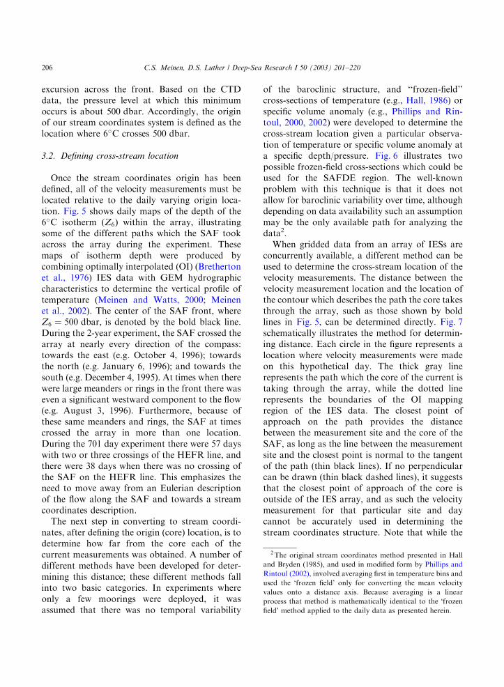
excursion across the front. Based on the CTDdata, the pressure level at which this minimumoccurs is about 500 dbar: Accordingly, the originof our stream coordinates system is defined as thelocation where 6�C crosses 500 dbar:

3.2. Defining cross-stream location

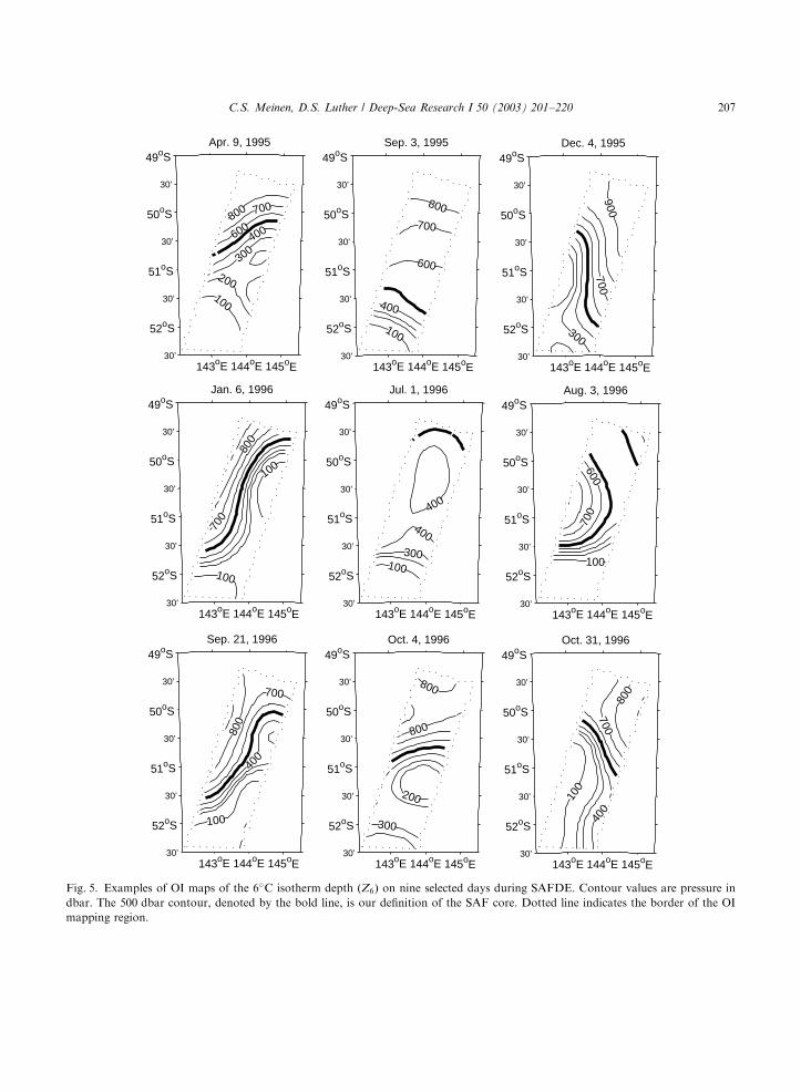
Once the stream coordinates origin has beendefined, all of the velocity measurements must belocated relative to the daily varying origin loca-tion. Fig. 5 shows daily maps of the depth of the6�C isotherm ðZ6Þ within the array, illustratingsome of the different paths which the SAF tookacross the array during the experiment. Thesemaps of isotherm depth were produced bycombining optimally interpolated (OI) (Brethertonet al., 1976) IES data with GEM hydrographiccharacteristics to determine the vertical profile oftemperature (Meinen and Watts, 2000; Meinenet al., 2002). The center of the SAF front, whereZ6 ¼ 500 dbar; is denoted by the bold black line.During the 2-year experiment, the SAF crossed thearray at nearly every direction of the compass:towards the east (e.g. October 4, 1996); towardsthe north (e.g. January 6, 1996); and towards thesouth (e.g. December 4, 1995). At times when therewere large meanders or rings in the front there waseven a significant westward component to the flow(e.g. August 3, 1996). Furthermore, because ofthese same meanders and rings, the SAF at timescrossed the array in more than one location.During the 701 day experiment there were 57 dayswith two or three crossings of the HEFR line, andthere were 38 days when there was no crossing ofthe SAF on the HEFR line. This emphasizes theneed to move away from an Eulerian descriptionof the flow along the SAF and towards a streamcoordinates description.

The next step in converting to stream coordi-nates, after defining the origin (core) location, is todetermine how far from the core each of thecurrent measurements was obtained. A number ofdifferent methods have been developed for deter-mining this distance; these different methods fallinto two basic categories. In experiments whereonly a few moorings were deployed, it wasassumed that there was no temporal variability

of the baroclinic structure, and ‘‘frozen-field’’cross-sections of temperature (e.g., Hall, 1986) orspecific volume anomaly (e.g., Phillips and Rin-toul, 2000, 2002) were developed to determine thecross-stream location given a particular observa-tion of temperature or specific volume anomaly ata specific depth/pressure. Fig. 6 illustrates twopossible frozen-field cross-sections which could beused for the SAFDE region. The well-knownproblem with this technique is that it does notallow for baroclinic variability over time, althoughdepending on data availability such an assumptionmay be the only available path for analyzing thedata2.

When gridded data from an array of IESs areconcurrently available, a different method can beused to determine the cross-stream location of thevelocity measurements. The distance between thevelocity measurement location and the location ofthe contour which describes the path the core takesthrough the array, such as those shown by boldlines in Fig. 5, can be determined directly. Fig. 7schematically illustrates the method for determin-ing distance. Each circle in the figure represents alocation where velocity measurements were madeon this hypothetical day. The thick gray linerepresents the path which the core of the current istaking through the array, while the dotted linerepresents the boundaries of the OI mappingregion of the IES data. The closest point ofapproach on the path provides the distancebetween the measurement site and the core of theSAF, as long as the line between the measurementsite and the closest point is normal to the tangentof the path (thin black lines). If no perpendicularcan be drawn (thin black dashed lines), it suggeststhat the closest point of approach of the core isoutside of the IES array, and as such the velocitymeasurement for that particular site and daycannot be accurately used in determining thestream coordinates structure. Note that while the

2 The original stream coordinates method presented in Hall

and Bryden (1985), and used in modified form by Phillips and

Rintoul (2002), involved averaging first in temperature bins and

used the ‘frozen field’ only for converting the mean velocity

values onto a distance axis. Because averaging is a linear

process that method is mathematically identical to the ‘frozen

field’ method applied to the daily data as presented herein.


Apr. 9, 1995

100

200

300400600

700800

143oE 144oE 145oE 30’

52oS

30’

51oS

30’

50oS

30’

49oS Sep. 3, 1995

100

400

600

700

800

143oE 144oE 145oE 30’

52oS

30’

51oS

30’

50oS

30’

49oS Dec. 4, 1995

300

700900

143oE 144oE 145oE 30’

52oS

30’

51oS

30’

50oS

30’

49oS

Jan. 6, 1996

700

100

100

800

143oE 144oE 145oE 30’

52oS

30’

51oS

30’

50oS

30’

49oS Jul. 1, 1996

100300

400

400

143oE 144oE 145oE 30’

52oS

30’

51oS

30’

50oS

30’

49oS Aug. 3, 1996

100

700

600

143oE 144oE 145oE 30’

52oS

30’

51oS

30’

50oS

30’

49oS

Sep. 21, 1996

800

700

400

100

143oE 144oE 145oE 30’

52oS

30’

51oS

30’

50oS

30’

49oS Oct. 4, 1996

300

200

800

800

143oE 144oE 145oE 30’

52oS

30’

51oS

30’

50oS

30’

49oS Oct. 31, 1996

100

400

700

800

143oE 144oE 145oE 30’

52oS

30’

51oS

30’

50oS

30’

49oS

Fig. 5. Examples of OI maps of the 6�C isotherm depth ðZ6Þ on nine selected days during SAFDE. Contour values are pressure in

dbar. The 500 dbar contour, denoted by the bold line, is our definition of the SAF core. Dotted line indicates the border of the OI

mapping region.


schematic illustration in Fig. 7 showed the path asa straight line, the path is more often curved likethe examples shown in Fig. 5; however, this is nota hindrance to the method described above.

The main advantage to determining the cross-stream distance in this manner is that no assump-tions regarding baroclinic time-invariance need tobe made. As such, the observations from this studycan be used to explore the time variability of thebaroclinic structure of the SAF. Fig. 8 (upperpanel) illustrates the wide variety of Z6 cross-sections observed during the 2 year SAFDE. TheZ6 at the HEFR sites were determined byvertically interpolating the temperature profilesestimated for each HEFR site on each day fromthe OI gridded IES t values and the temperatureGEM field. On each day the maximum number of

Z6 estimates possible was seven (one at eachHEFR site), so to obtain more complete cross-sections spatial gaps in cross-stream location of upto 50 km were interpolated. Only days which hadat least four Z6 measurements, and where therewere measurements spanning the core, wereplotted. The mean Z6 cross-section is also shown.

ue

ve

us

vs

Schematic of stream-coordinates calculations

Fig. 7. Schematic demonstrating the OI method for determin-

ing cross-stream distance and downstream angle. The bold gray

line represents the core of the current, while the dotted line

represents the boundary of the OI mapping region (similar to

Fig. 5). Open circles represent HEFR sites, and thin black lines

are the perpendicular lines drawn between the HEFR sites and

the closest point on the idealized SAF core. Dashed lines

demonstrate that perpendicular lines cannot be drawn between

the two southernmost HEFRs and the closest point on the core

contour on this particular day. The black pair of arrows

indicate east ðueÞ and north ðveÞ directions in geographic

coordinates, while the gray pair of arrows demonstrates

downstream ðusÞ and cross-stream ðvsÞ for this idealized case.

Because in reality the core contour would not generally pass

through the mapping region as a straight line, the actual

orientation of downstream would be determined independently

for each HEFR site based on a tangent line to the core at the

point where the perpendicular line (thin black lines) intersected

the core (bold gray line).

-50 0 50 100

0

200

400

600

800

Z6 [d

bar]

Possible frozen field distance axes

-50 0 50 100

7

8

9

10

11

12

δ 780 [1

0 -7

m3 k

g -1]

Cross-stream distance [km]

Fig. 6. Possible frozen field distance axes; upper panel shows a

canonical cross-stream section of the 6�C isotherm pressure,

while the lower panel shows a cross-section of the specific

volume anomaly at 780 dbar: The latter is similar to the frozen-

field axis used by Phillips and Rintoul (2002).


The lower panel of Fig. 8 demonstrates thevariability in Z6 slopes with the gray line andband, which represent the mean slope plus orminus one standard deviation. Near the center ofthe SAF this range of observed slopes representsapproximately a factor of 2 deviation from themean in either direction (smaller or larger).

The variability shown in Fig. 8 suggests largebaroclinic changes occurred during the 2-yearexperiment. It could be argued, however, that the

variability in the slope in Fig. 8 results fromthe interpolation needed to obtain cross-sectionsfrom only 4–7 observations of Z6 on a givenday. To confirm that this observed variabilityin slope is not due simply to the limited samplingand interpolation necessary to fill gaps betweenmeasurements, 7100 random four point sub-samples of the mean observed Z6 cross-sectionwere made (i.e. over 10 times the number ofactual daily samples). For each four point sample,gaps smaller than 50 km were filled and onlysamples which had ‘‘observations’’ on either sideof the core were used. The mean and standarddeviation of the resulting slopes are shown in thelower panel of Fig. 8. The variability induced bysampling is much smaller than the observed slopevariability, demonstrating that the majority of thevariability shown by the gray area must be actualocean variability. The mean values from therandom samples are slightly lower than the meanof the observed Z6 slopes because randomsampling and interpolation can only smooth themean curve.

Fig. 8 suggests that assuming no temporalvariability of the baroclinic structure for the flowalong the SAF would result in significant errors indetermining cross-stream location. In order toquantify this error, the specific volume anomalyalong 780 dbar (d780) cross-section from Fig. 6 wascombined with the estimated d780 on each day atthe HEFR sites to determine the cross-streamlocation which would have been obtained underthe assumption of no baroclinic temporal varia-bility. The cross-stream distance estimated in thismanner is compared (Fig. 9a) to the distancedetermined using the OI mapped Z6 field asdiscussed previously. The differences between thetwo estimates of distance are small near the core,but they increase rapidly further from the core(Fig. 9b). While the two quantities roughly followthe 1-1 line, the scatter is quite large. Fig. 9bdetails the root-mean-square (RMS) differenceswithin 10 km wide bins. At 20 km from the coreon either side of the front the RMS differencesexceed 10 km; and by 40 km from the core thedifferences exceed 20 km; demonstrating the largeerrors which would result from assuming a time-invariant Z6 cross-section.

-80 -60 -40 -20 0 20 40 60 80 100 120

0

200

400

600

800

1000

Pre

ssur

e [d

bar]

Observations of 6°C isotherm depth in stream coordinates

-80 -60 -40 -20 0 20 40 60 80 100 120 2

0

2

4

6

8

10

12


Isot

herm

slo

pe [×

10

-3]

Observations of 6°C isotherm slope in stream coordinates

Fig. 8. Upper panel: The observed cross-sections of 6�C

isotherm depth (gray lines) during SAFDE, see text for details

of determination. The bold black line represents the mean of the

gray lines. Lower panel: The gray line and band represent the

mean and range of the observed cross-stream slopes of the 6�C

isotherm depth (mean plus and minus one standard deviation).

The open black circles and associated error bars represent the

scatter due to subsampling errors (see the text for detail).


These errors in stream coordinates distance willhave essentially no effect at the core of the SAF,but away from the core they tend to smooth thecross-section. To demonstrate this effect, anidealized along-stream velocity cross-section basedon a Gaussian (normal) function was created(Fig. 10a). The idealized cross-stream flow wasbased on a hyperbolic tangent, which simplysimulates a divergent current. To simulate theeffect of distance errors on the idealized cross-section, a series of random values was generatedfor each distance grid point along the cross-section. The magnitude of the random valueswas set so that the RMS value of the randomvalues was equal to the corresponding value froma linear fit to the RMS differences shown inFig. 9b. The number of random values at each gridpoint was given by a linear model with 300 samplesin the central bin and dropping to 20 by 7120 km;simulating the real distribution of observations.The random distance errors, combined with the‘correct’ distance for a particular bin, were used toextract a ‘‘time series’’ of velocities from the

idealized cross-sections. The resulting erroneoussimulated velocity values were then averaged andthe difference between that average and theidealized velocity at that distance grid pointprovides an estimate of the impact of using atime-invariant baroclinic structure for determiningcross-stream distance. The resulting mean velocitycross-section agrees well with the correct cross-section near the core of the current; however,significant smoothing and increased transportresults near the flanks of the current (Fig. 10a).Based on the realistic values used in this simula-tion, the transport which would be calculatedunder the assumption of no baroclinic variabilitywould be about 12% too large. Furthermore,energetics studies frequently require estimates ofthe cross-stream gradient of along-stream velocity(e.g. Kontoyiannis, 1997); it is evident fromFig. 10a that estimates of that gradient will beweakened on the flanks of the current and thecurrent will also appear artificially wide. While theassumption of no baroclinic variability is indeedthe only way to obtain stream coordinates

-80 -40 0 40 80 120

-80

-40

0

40

80

120D

ista

nce

from

‘fro

zen’

δ 780 [k

m]

-80 -40 0 40 80 1200

10

20

30

40

50

60

Distance from OI mapped Z6 [km]

RM

S d

ista

nce

diffe

renc

e [k

m]

-150 -50 50 150

-150

-100

-50

0

50

100

150

Ang

le fr

om v

ertic

al s

hear

-150 -50 50 15010

20

30

40

50

60

Angle from OI mapped Z6 [km]

RM

S a

ngle

diff

eren

ce

-80 -40 0 40 80 120

-150

-100

-50

0

50

100

150

Ang

le d

iffer

ence

-80 -40 0 40 80 120

-150

-100

-50

0

50

100

150

Distance from OI mapped Z6 [km]

Mea

n an

gle

diffe

renc

e [k

m]

(a) (c) (e)

(f)(d)(b)

Fig. 9. Stream coordinates methods: (a) comparison of cross-stream distance determined using frozen-field distance versus using OI

mapped 6�C depths; (b) RMS distance differences from (a) determined in 10 km wide bins; (c) comparison of downstream angle

determined using the direction which maximizes the vertical shear of horizontal velocity versus the downstream angle determined from

the OI mapped 6�C depths (0� represents East); (d) RMS differences from (c) determined in 10� wide bins; (e) difference in angle from

(c) as a function of cross-stream distance; (f) mean angle differences from (e) averaged in 10 km wide bins. All quantities calculated

from SAFDE data.


information from a limited number of moorings,the results shown here suggest that resultsobtained from such calculations must be inter-preted with caution, at least in the SAF.

3.3. Determining downstream direction

For the final step in moving into streamcoordinates, rotating the velocities, there alsoare basically two methods which have been appliedin the past: defining the downstream directionas the direction which locally maximizes thevertical shear of the horizontal velocities; andusing other horizontally gridded information, suchas thermocline depth determined from IESs, todetermine the downstream direction (Johns et al.,1995; Bower and Hogg, 1996). The former methodmust be used when data from just a few mooringsare available, the latter can be adopted onlywhen there is a large array of moorings. Johnset al. (1995) describe both methods in somedetail in a stream coordinates application tocurrent meter mooring measurements in theGulf Stream near 68�W: In that study the verticalshear method was used whenever the differencebetween current meter measured velocities at400 and 1000 m exceeded 5 cm s�1: When theshear was smaller, the direction was determinedby following the path of the 12�C isothermcrossing 400 dbar through the array. Johns andcoauthors calculated the 12�C isotherm depth fieldfrom the measurements of an array of IESs whichsurrounded and overlapped the current metermooring array.

-120 -80 -40 0 40 80 120-20

-10

0

10

20

30

40

50

60

Vel

ocity

[cm

s -1]

Vel

ocity

[cm

s -1]

Vel

ocity

[cm

s -1]

Simulation of distance errors

Uim

Vim

Uff

Vff

-120 -80 -40 0 40 80 120 -20

-10

0

10

20

30

40

50

60 Simulation of "local versus core" angle errors

Uim

Vim

Uvs

Vvs

-120 -80 -40 0 40 80 120 -20

-10

0

10

20

30

40

50

60


Simulation of "divergence" angle errors

Uim

Vim

Udiv

Vdiv

(a)

(b)

(c)

Fig. 10. Simulating the errors induced by using the frozen-field

cross-stream distance method and/or the vertical shear method

of determining downstream direction. For all panels the bold

black (along-stream) and gray (cross-stream) lines represent a

simple idealized model velocity cross-section at a particular

depth. The thin lines simulate the cross-sections which would be

obtained under the following situations: (a) using the frozen

field distances but the OI method for determining the down-

stream angle; (b) using the OI method distances but including a

random downstream direction error due to using the local

vertical shear for determining the downstream angle; (c) using

the OI method distances but rotating the cross-stream flows

into along-stream to simulate an angle bias error similar to

what is shown in Fig. 9f.


There are two potential problems with using thevertical shear method for finding the direction ofdownstream. First, the presence of eddies andrings within and near the current suggests that thedirection of strongest shear at a particular moor-ing location may not be parallel to the downstreamdirection some distance away at the core of thecurrent. This represents a random angle errorwhich can occur anywhere across the current.Second, the presence of recirculation gyres oneither side of a current, well documented in theGulf Stream (Hogg, 1992) and likely presentaround the ACC as well, indicates that away fromthe current core axis there is either a divergentcomponent or a convergent component to thewater velocity due to the divergence or conver-gence of the recirculation cells. This implies thatthe direction of largest shear, at locations awayfrom the core axis, may not be parallel to the coreif there is a baroclinic component to the recircula-tion cells. The result would be a bias with allobserved angles on one side of the current havingerrors of one sign and all observed angles on theother side of the current having errors of theopposite sign.

Consider first the former (random angle) pro-blem. Fig. 9c shows a comparison of the down-stream angle as determined from the velocity shearmethod to the angle as determined from the OImapped Z6 field as shown in Fig. 7. There is asuggestion of a 1-1 correspondence in general;however the scatter is quite large. There is noparticular pattern to the differences (Fig. 9d),which is not surprising considering the possiblecombinations of a widely varying downstreamdirection (e.g. Fig. 5) with randomly located eddiesand rings. The effect of a random angle error onan idealized current in the presence of a cross-stream divergence is mainly a reduction in thealong-stream velocity in the core of strongvelocities; the effect on the cross-stream velocitiesis roughly the same on a percentage basis, butgiven the smaller magnitude of the cross-streamflow the effects are primarily noted as a slightweakening of the mean divergence and theintroduction of a small amount of noise (Fig. 10b).

A more diagnostic test is to look at thedifferences in angle as a function of cross-stream

distance (Fig. 9e). While there is still a great deal ofscatter in the individual observations, by binaveraging the observed distances a distinct biasingpattern emerges (Fig. 9f). This pattern is statisti-cally significant at the 95% confidence level. Forlocations on the warm side of the SAF core(positive distances in Fig. 9f), the differences arenegative, indicating that the shear method gives adownstream direction which is rotated counter-clockwise of that given by the OI mapped values.For locations on the cold side of the front theresult is the opposite. This suggests that by usingthe OI mapped Z6 method the resulting cross-stream divergence will be larger than that whichwould be determined from the velocity shearmethod. By 50 km from the core this angledifference is 10–20�; which is quite significant.The effect of an angle bias error on the idealizedalong-stream current (Fig. 10c) is small near thecore of the current, but it artificially increases theflows out near the flanks of the current. The cross-stream flows are zero if the entire cross-streamcomponent is rotated into along-stream.

Bower and Hogg (1996) documented anotherdanger of using the vertical shear method todetermine downstream direction. Their GulfStream study found a curvature-dependent angleoffset between the vertical shear and OI-mappedmethods; the vertical shear method consistentlydemonstrated equatorward cross-stream flowwhen transitioning from a meander crest to atrough and poleward flow when changing fromtrough to crest. They pointed out that this flow isnot related to inflow or outflow from recircula-tions outside of the Gulf Stream and as such thevertical shear method should not be used ifassessing these convergences or divergences is agoal of the study.

3.4. Optimum method for defining stream

coordinates

Herein follows the optimum conversion tostream coordinates as proposed in this study.For each day of the time series, Z6 was contouredthrough the array using the IES data. Then, foreach site on each day, the closest point on the Z6 ¼500 dbar contour was found and, if the line


between that point and the HEFR site was within10� of perpendicular to a tangent to the contour,the point was defined as the location of the corefor that HEFR site for that day. The distancebetween the two points was defined as the cross-stream distance (positive if the 6�C isotherm at theHEFR site was deeper than 500 dbar; negative if itwas shallower), while the tangent to the contourline provided the direction of downstream forrotation of the velocities into along-stream andcross-stream components. This process was re-peated for each of the seven HEFR within themain array, and then the processing continued onto the next day of the time series and the procedurerepeated. For situations where the closest point onthe contour was less than 3 km away from theHEFR site, the distance was set to 0 km and thetangent at the closest point provided the definitionof downstream. For situations where the choice ofa closest point was particularly ambiguous, such aswhen two points on the contour were nearlyequidistant from the HEFR site, the data fromthat site on that day were not used in developingthe stream coordinates mean.

Of the 4907 absolute velocity profiles (7 HEFRsites times 701 days), 3100 could be used indetermining the stream coordinates mean. Forthe remaining profiles, their particular sites werelocated relative to the SAF core such that theclosest approach of the SAF was either outside theIES array (see Fig. 7) or was ambiguously defined,and therefore the cross-stream location and down-stream direction could not be determined. (Notethat the frozen-field method and local verticalshear methods do not have these restrictions, andtherefore can utilize all 4907 profiles. This does notlead to better results, as will be shown shortly.)The usable velocity estimates, as well as thetemperature and salinity estimates at those sitesas determined from the IES gridded t values andthe GEMs, were averaged in 10 km wide binscentered at 10 km intervals from the streamcoordinates core. The resulting mean sections weresmoothed slightly using a 40 km low-pass filter(second-order Butterworth filter passed both for-ward and back to avoid phase shifting) in order tofacilitate the intercomparisons of the varioussections (smoothing is not applied for dynamical

studies; see Meinen et al., submitted for publica-tion). No vertical smoothing was applied. Thenumber of velocity observations used in the streamcoordinates averaging ranged from about 10observation-days for the bins 150 km from thecore to about 300 observation-days at the core.Only bins with at least 20 observation-days wereconsidered to have useful means, which restrictedthe usable range to within 90 km on the cold sideof the SAF and to within 120 km on the warm sideof the front.

4. Results

Fig. 11 presents the stream coordinates meanalong- and cross-stream velocity produced whenthe OI mapped Z6 field is used for determiningboth the downstream direction and the cross-stream distance. The peak along-stream velocitiesare about 50 cm s�1 at the surface, and at4000 dbar the peak velocities reach 2 cm s�1: Thealong-stream velocities have a single peak, similarto other oceanic jets such as the Gulf Stream(Johns et al., 1995) and the North Atlantic Current(Meinen, 2001). Those other currents, however,clearly have a more asymmetric structure and anequatorward displacement of the velocity max-imum with increasing depth, neither of which isvery evident in the SAF. The cross-stream flow isdivergent both baroclinically and (weakly) baro-tropically, with peak velocities of 8–10 cm s�1 nearthe surface and near bottom velocities of about 1–2 cm s�1: [N.B. barotropic is defined as the nearbottom velocity following Fofonoff (1962).] Theequatorward flow on the warm side of the SAF isconsistent with the anticyclonic recirculation northof the front as proposed by Rintoul et al. (2001) onthe basis of repeated hydrographic sections;however, the poleward flow on the cold side ofthe SAF does not correspond in an obvious way tothe circulation picture proposed by those authors.The mean absolute transport along the SAF,integrated from the bottom to the surface andbetween the 10 km wide bins centered at �90 andþ120 km; was 75 Sv (Sv: 106 m3 s�1).

Consider next the results of determiningthe stream coordinates mean using the ‘correct’


-80 -60 -40 -20 0 20 40 60 80 100 120

0

500

1000

1500

2000

2500

3000

3500

4000

Pre

ssur

e [d

bar]

5

10

1520

25 30

35 4045

-80 -60 -40 -20 0 20 40 60 80 100 120

0

500

1000

1500

2000

2500

3000

3500

4000

Pre

ssur

e [d

bar]

2 4

6 8

24

6

10

-80 -60 -40 -20 0 20 40 60 80 100 120

0

500

1000

1500

2000

2500

3000

3500

4000

Cross-stream distance [km] Cross-stream distance [km]


Pre

ssur

e [d

bar]

Standard deviation of Uoi [cm s-1] Standard deviation of Voi [cm s-1]

Mean Voi [cm s-1] Mean Uoi [cm s-1]

5

10

5

15

20

-80 -60 -40 -20 0 20 40 60 80 100 120

0

500

1000

1500

2000

2500

3000

3500

4000

Pre

ssur

e [d

bar]

4

610

14

18

8 10

12 10

2

4

6

8

10

12

14

16

18

20

Deg

rees

of f

reed

om (

dash

ed li

ne)

-80 -60 -40 -20 0 20 40 60 80 100 1200

50

100

150

200

250

300

350

Num

ber

of o

bser

vatio

ns (

solid

line

)

Observations and degrees of freedom

(a) (b)

(d)

(e)

(c)

Fig. 11. (a) The along-stream mean current section from stream coordinates using the OI method for both downstream direction and

cross-stream distance definitions; (b) the cross-stream mean current section from stream coordinates using both OI stream coordinates

definitions; (c) the standard deviation of the along-stream current; (d) the standard deviation of the cross-stream current; (e) solid line

shows the number of absolute velocity profile observations used in the averaging within each 10 km bin, dashed line shows the

estimated number of degrees of freedom within each 10 km wide bin. In panels (a)–(d) the solid contours indicate positive flow, dashed

contours indicate negative flow, and the bold contour indicates zero flow. Contours are in cm s�1: Note along-stream and cross-stream

currents have different contour intervals.


rotation angle as determined from the OI mappedZ6 field but estimating the cross-stream distanceusing the ‘frozen-field’ structure of d780 (Fig. 12).The resulting stream coordinates mean along-stream velocity displays two maxima in the upper1000 dbar: The current structure is significantlydifferent from that of the ‘correct’ section shownin Fig. 11, with a smearing of the velocity signals

over larger horizontal distances and a 30 kmnorthward shift of the deep velocity maximum.The cross-stream flow, by contrast, is fairly similarbetween the sections shown in Figs. 11 and 12.This is consistent with the idealized results shownearlier (Fig. 10a).

If instead the stream coordinates mean isdetermined using the ‘correct’ OI mapped cross-stream distances but using the local vertical shearfor downstream direction, the resulting along-stream flow (Fig. 13) is very similar to the ‘correct’estimates from Fig. 11 near the SAF core. Awayfrom the core, however, the use of the local verticalshear direction results in stronger along-streamflows. This is to be expected because the cross-stream flows in Fig. 11 are rotated into along-stream flows in Fig. 13. The cross-stream flows inFig. 13 are generally very small, with no significantbaroclinicity in the cross-stream flow because ofthe direction definition. The resulting along-streamtransport from Fig. 13 exceeds that of Fig. 11 by10%, while the cross-stream transports are ob-viously much smaller when the vertical shear isused for the direction.

A final comparison is made to the streamcoordinates mean velocity sections which wereobtained by using the ‘frozen-field’ distances andthe vertical shear directions, e.g. the ‘wrong’methods for both distance and direction(Fig. 14). The general patterns of Figs. 12 and 13are evident in Fig. 14: multiple along-streamvelocity peaks, little cross-stream flow, broad andlarge along-stream transports. With limited data,such as a few current meters, and no OI mappedfield of IESs, the only stream coordinates meansection which could have been obtained for theSAF in this region would be similar to the oneshown in Fig. 14. However, because of theavailability of the OI mapped Z6 fields for derivingcross-stream distances and rotation angles, it hasbeen possible to document that the ‘true’ streamcoordinates section is that shown in Fig. 11. Thesignificant differences between the two sections(Figs. 11a, b and 14) raise questions about whetherdetermining the stream coordinates mean from alimited number of moorings is a viable approach.Extracting cross-sections at several depth levelsfrom each of the sections shown in Figs. 11–14

-80 -40 0 40 80 120

0

500

1000

1500

2000

2500

3000

3500

4000

Pre

ssur

e [d

bar]

5

10

1520

25 30

3535

-80 -40 0 40 80 120

0

500

1000

1500

2000

2500

3000

3500

4000


Pre

ssur

e [d

bar]

Vff [cm s -1]

Uff [cm s-1]

2

4 6 8

2

4

86

Fig. 12. The along-stream (upper panel) and cross-stream

(lower panel) stream coordinates mean sections obtained using

the OI method for determining downstream direction but the

frozen field method for determining cross-stream distance. Solid

contours indicate positive flow, dashed contours indicate

negative flow, bold contour indicates zero flow. Contours are

in cm s�1: Note along-stream and cross-stream velocities have

different contour intervals.


emphasizes further (Fig. 15) that the use of eitherthe ‘frozen-field’ method of determining cross-stream distance or the use of the local vertical shearof horizontal velocity for determining the down-stream direction results in inaccurate estimates forthe along-stream velocity means in the SAF. It willbe shown shortly that these differences can haveimportant impacts on the dynamical interpretationof the stream coordinates mean section.

4.1. Optimum method results

Fig. 11a presents the ‘correct’ mean along-stream absolute velocity for the SAF, along withthe standard deviation (Fig. 11c) and the numberof daily velocity profiles which were used withineach 10 km wide averaging-bin (Fig. 11e). Thestandard deviations of the along-stream velocitiesdemonstrate that the strength of the ACC flow

-80 -40 0 40 80 120

0

500

1000

1500

2000

2500

3000

3500

4000

Pre

ssur

e [d

bar]

5

10

1520

25 30

35 45

-80 -40 0 40 80 120

0

500

1000

1500

2000

2500

3000

3500

4000


Pre

ssur

e [d

bar]

11

Uvs [cm s -1]

Vvs [cm s -1]



the OI method for determining cross-stream distance but the

vertical shear method for determining downstream direction.

Solid contours indicate positive flow, bold contour indicates

zero flow. Contours are in cm s�1: Note along-stream and cross-

stream velocities have different contour intervals.

-80 -40 0 40 80 120

0

500

1000

1500

2000

2500

3000

3500

4000

5

10

15 20

25 3035

35

-80 -40 0 40 80 120

0

500

1000

1500

2000

2500

3000

3500

4000


Pre

ssur

e [d

bar]

P

ress

ure

[dba

r]

Vffvs [cm s -1]

Uffvs [cm s -1]



the vertical shear method for determining downstream direction

and the frozen-field method for determining cross-stream

distance. Solid contours indicate positive flow, bold contour

indicates zero flow. Contours are in cm s�1: Note along-stream

and cross-stream velocities have different contour intervals.


along the SAF changes significantly, with the coreat the surface having a standard deviation of about25 cm s�1: Since the effect of meandering isremoved from the stream coordinates referenceframe, the baroclinic nature of the standarddeviations suggests that there was a significantamount of baroclinic variability observed duringthe experiment, consistent with Fig. 8.

The cross-stream mean absolute velocities(Fig. 11b) and standard deviations (Fig. 11d)demonstrate that the divergence, with northwardflow north of the core and southward flow to thesouth, was quite variable during the experiment.The mean divergence pattern is statistically sig-nificant, however, even though the meanderpatterns (and hence the curvature) were so variableduring SAFDE (e.g. Fig. 5).

Before continuing, a brief discussion of themeasurement accuracy of these velocity estimatesis in order. Meinen et al. (2002) quantify theaccuracy in the absolute velocities derived from theIES and HEFR measurements to be 8, 6, 4, and3 cm s�1 for pressures of 300, 600, 1000, and2000 dbar; respectively. These one standard devia-tion error bars are for the daily velocity measure-ments and they were determined by comparisonwith several current meters involved in SAFDE aswell as other independent data. In order todetermine the accuracy of the stream coordinatesmean values shown in Fig. 11 an estimate of thedegrees of freedom must be made. Johns et al.(1995) showed that the number of degrees offreedom in a stream coordinates reference framewas essentially the same as the number in anEulerian reference frame. This makes sense,

-50 0 50 1000

10

20

30

40

50

60

Alo

ng-s

trea

m v

el. a

t 400

dba

r [c

m s

-1]

Alo

ng-s

trea

m v

el. a

t 110

0 db

ar [c

m s

-1]

Alo

ng-s

trea

m v

el. a

t 350

0 db

ar [c

m s

-1]

Uoi

Uff

Uvs

Uffvs

-50 0 50 1000

5

10

15

20

25

30U

oiU

ffU

vsU

ffvs

-50 0 50 100 -5

0

5

10


Uoi

Uff

Uvs

Uffvs

Fig. 15. A comparison of the stream coordinates mean

velocities from Figs. 11–14 at three depth levels; 400, 1100,

and 3500 dbar (top, middle, bottom). Legend shows to which

mean section each line corresponds; ‘‘oi’’ indicates the OI

method was used for both downstream angle and cross-stream

location (Fig. 11), ‘‘ff’’ indicates OI method was used for

downstream direction but frozen-field method was used for

cross-stream location (Fig. 12), ‘‘vs’’ indicates OI method was

used for cross-stream location but vertical shear method was

used for downstream direction (Fig. 13), ‘‘ffvs’’ indicates

frozen-field method was used for cross-stream location and

vertical shear method was used for downstream direction

(Fig. 14).


because although moving to a stream coordinatesreference frame eliminates the horizontal motionof the meanders, it does not eliminate the changesin thermocline slope which are associated withthose meanders (e.g. Fig. 10 of Watts et al., 1995).The number of degrees of freedom across the sec-tion was determined as follows. First, the integraltime scale was determined at each of the HEFRsites (Emery and Thomson, 1997), resulting inan average integral time scale of about 11 days.Next, because the ‘time series’ of points availablein each bin of the stream coordinates section wasirregular (ranging from 3–4 points in a single binon a given day, if the SAF was running parallel tothe HEFR line that day, to no observations in aparticular bin for weeks), it was necessary to breakup the time series for each cross-stream bin intosections one integral time scale in length and thendetermine how many of the sections containedobservations. The resulting number of degrees offreedom ranged from 6 to 20, with the fewestnumber on the warm side of the SAF and thelarger number on the cold side of the SAF(Fig. 11e). Near the SAF core there were about14 degrees of freedom, which indicates that themeasurement errors contribute at most 1–2 cm s�1

to the error in the stream coordinates mean. Thestatistical standard error of the mean ranges from2 cm s�1 at 2000 dbar to 7 cm s�1 near the surfacefor the along-stream velocities and 1 cm s�1 at2000 dbar to 2 cm s�1 near the surface for thecross-stream velocities. Therefore, the mean velo-cities shown in Fig. 11 are accurate to within 1–7 cm s�1 over the full water column.

4.2. Example of dynamical implications

The descriptive differences between the streamcoordinates mean sections shown in Figs. 11–14also have an impact on dynamical conclusionswhich are drawn from the sections. A morecomplete discussion of the dynamics of the SAFbased on the stream coordinates mean section willbe presented in a future paper (Meinen et al.,submitted for publication), but one example ispresented here.

Analytical and numerical models of an inertialjet suggest that the cross-stream gradient of the

along-stream velocity should have a larger magni-tude on the cold side of the current (Fofonoff andHall, 1983; Hall, 1986; Smith et al., 2000).Previous observational estimates of the streamcoordinates sections have found conflicting resultsin this regard. Johns et al. (1995) found that thelargest horizontal shear magnitude occurred onthe cold side of the Gulf Stream, consistent withthe analytical model. Hall (1986) instead found thehorizontal shear magnitude to be larger on thewarm side of the Gulf Stream at a location fairlyclose to the later Johns et al. (1995) study. Phillipsand Rintoul (2002) found the largest horizontalshear magnitude on the warm side of the SAF. Theresults from our best section indicate that thelargest horizontal shear magnitude is on the coldside of the SAF (Fig. 16), although the asymmetryis weak. In order to explain these disagreementsfor both the Gulf Stream and for the SAF it isnecessary to compare the methods used in devel-oping each of these stream coordinates meansections. The Hall (1986) Gulf Stream sectionutilized distances determined under a ‘frozen field’assumption and downstream directions deter-mined from the local vertical shear of horizontalvelocity. The Phillips and Rintoul (2002) SAFsection did the same. The Johns et al. (1995) GulfStream section utilized distances from an OImapped Z12 field similar to our use of a mappedZ6 field in the SAF (the 12�C isotherm is withinthe main thermocline in the Gulf Stream). Forrotating the velocity observations into along-stream and cross-stream components, the Johnset al. (1995) study used a hybrid of the twomethods presented earlier; when the local velocityshear exceeded a certain criterion it was used todefine the downstream direction, otherwise themapped Z12 field was used.

The Hall (1986) Gulf Stream section andPhillips and Rintoul (2002) SAF section usedsimilar methods, and both observed the strongermagnitude of cross-stream shear of along-streamvelocity on the warm side of the respectivecurrents, counter to the analytical model results.The Johns et al. (1995) Gulf Stream section andour SAFDE section used generally similar meth-ods and both studies found that the strongermagnitude of cross-stream shear of along-stream


velocity was on the cold side of the front,consistent with the analytical model results.Rossby and Zhang (2001) used a cross-streamdistance and downstream direction method similarto the SAFDE study, with the core defined by thelocation and direction of the velocity maximumrather than an isotherm crossing a pressure

surface, in a study of repeat ADCP sections acrossthe Gulf Stream and they also found the highestshear magnitude on the cold side of the current.While not completely definitive (further studies arerequired since the Johns et al. (1995) study used aslightly different method than in this study and theRossby and Zhang (2001) study did not allow forstream curvature), these results suggest that theuse of the ‘frozen-field’ and vertical shear methodsprovides an erroneous result. Hogg (1992), on theother hand, revisited the Hall (1986) data andsuggested that the particular definition of frozencross-stream distance used by Hall (1986) mighthave resulted in obtaining the strongest shearmagnitude on the ‘wrong’ side of the Gulf Stream.This ambiguity in frozen field results highlightsboth the importance of the method used indeveloping stream coordinates mean sections andalso the need for caution in interpreting streamcoordinates mean sections previously developedusing strong assumptions about the character ofthe flow and its variability. While studies such asHall (1986) and Phillips and Rintoul (2002)provided considerable improvements over pre-vious Eulerian mean estimates of the structure ofthe Gulf Stream and SAF respectively, dynamicalinterpretation may be better left to streamcoordinates sections developed using a morerobust method such as those of Johns et al.(1995) and this study.

Acknowledgements

The authors would like to thank RandyWatts and Karen Tracey for providing theOI mapped inverted echo sounder data andsome of the hydrography used in this experiment.Alan Chave kindly provided the final calibratedHEFR data, while Steve Rintoul provided someof the hydrography used in the study. RandyWatts, Karen Tracey, Steve Rintoul, HelenPhillips, Tom Rossby and an anonymousreviewer made many helpful suggestions forimproving the manuscript. This study was fundedunder NSF grant numbers OCE92-04113 andOCE99-11974.

-20 -10 0 10 20 30 40

0

500

1000

1500

2000

2500

3000

3500

4000

Pre

ssur

e [d

bar]

P

ress

ure

[dba

r]

∂Uoi

/∂y [10 -6 s -1 ]

6 4 3

2

∂Uffvs /∂y [10 -6 s -1 ]

1

1

1

1

2

35

610 20 30 40 50 60 70

0

500

1000

1500

2000

2500

3000

3500

4000


2 11

2

Fig. 16. Cross-stream gradient of the stream coordinates mean

along-stream component of the absolute velocity. Dashed

contours indicate negative, solid indicates positive. Upper

panel shows the gradient of the mean section determined using

the OI-mapped distance and direction (Fig. 11), lower panel

shows the gradient of the mean section determined using the

frozen-field location and vertical shear downstream direction

(Fig. 14).


References

Bower, A.S., Hogg, N.G., 1996. Structure of the Gulf Stream

and its recirculations at 55� W: Journal of Physical

Oceanography 26, 1002–1022.

Bretherton, F.P., Davis, R.E., Fandry, C.B., 1976. A technique

for objective analysis and design of oceanographic experiments

applied to MODE-73. Deep-Sea Research I 23, 559–582.

Chaplin, G.F., Watts, D.R., 1984. Inverted echo sounder

development. IEEE Oceans ’84 Conference Record, Vol. 1,

pp. 249–253.

Chave, A.D., Luther, D.S., 1990. Low-frequency, motionally

induced electromagnetic fields in the ocean: 1. Theory.

Journal of Geophysical Research 95, 7185–7200.

Chave, A.D., Luther, D.S., Meinen, C.S. Correction of

motional electric field measurements for galvanic distortion.

Journal of Atmospheric and Oceanic Technology, sub-

mitted for publication.

Emery, W.J., Thomson, R.E., 1997. Data Analysis Methods in

Physical Oceanography. Pergamon Press, Oxford.

Fofonoff, N.P., 1962. Dynamics of ocean currents. In: Hill,

M.N. (Ed.), The Sea: Ideas and Observations on Progress in

the Study of the Seas, 1: Physical Oceanography. Wiley-

Interscience, New York, pp. 323–395.

Fofonoff, N.P., Hall, M.M., 1983. Estimates of mass,

momentum and kinetic energy fluxes of the Gulf Stream.

Journal of Physical Oceanography 13, 1868–1877.

Gille, S.T., 1994. Mean sea surface height of the Antarctic

Circumpolar Current from Geosat data: Method

and application. Journal of Geophyiscal Research 99,

18255–18273.

Halkin, D., Rossby, H.T., 1985. The structure and transport of

the Gulf Stream at 73� W: Journal of Physical Oceano-

graphy 15, 1439–1452.

Hall, M.M., 1986. Horizontal and vertical structure of the Gulf

Stream velocity field at 68� W: Journal of Physical


Hall, M.M., 1989. Velocity and transport structure of the

Kuroshio extension at 35� N; 152� E: Journal of Geophy-

sical Research 94, 14445–14459.

Hogg, N.G., 1992. On the transport of the Gulf Stream between

Cape Hatteras and the Grand Banks. Deep-Sea Research I

39, 1231–1246.

Johns, W.E., Shay, T.J., Bane, J.M., Watts, D.R., 1995. Gulf

Stream structure, transport, and recirculation near 68� W:Journal of Geophysical Research 100, 817–838.

Kontoyiannis, H., 1997. Quasi-geostrophic modeling of mixed

instabilities in the Gulf Stream near 73� W: Dynamics of

Atmospheres and Oceans 26, 133–158.

Luther, D.S., Filloux, J.H., Chave, A.D., 1991. Low-frequency,

motionally induced electromagnetic fields in the ocean: 2.

Electric field and eulerian current comparison. Journal of

Geophysical Research 96, 12797–12814.

Luther, D.S., Chave, A.D., Church, J.A., Filloux, J.H.,

Richman, J.G., Rintoul, S.R., Watts, D.R., 1997. The

sub-antarctic flux and dynamics experiment (SAFDE).

WOCE Notes 9, 8–12.

Meinen, C.S., 2001. Structure of the North Atlantic Current in

stream-coordinates and the circulation in the Newfound-

land Basin. Deep-Sea Research I 48, 1553–1580.

Meinen, C.S., Watts, D.R., 2000. Vertical structure and

transport on a transect across the North Atlantic Current

near 42� N: time series and mean. Journal of Geophysical

Research 105, 21869–21891.

Meinen, C.S., Luther, D.S., Watts, D.R., Chave, A.D., Tracey,

K.L. Mean stream-coordinates structure of the Subantarctic

Front: temperature, salinity, and absolute velocity. Journal

of Geophysical Research, submitted for publication.

Meinen, C.S., Luther, D.S., Watts, D.R., Tracey, K.L., Chave,

A.D., Richman, J., 2002. Combining Inverted Echo

Sounder and Horizontal Electric Field Recorder measure-

ments to obtain absolute velocity profiles. Journal of

Atmospheric and Oceanic Technology 19, 1653–1664.

Phillips, H.E., Rintoul, S.R., 2000. Eddy variability and

energetics from direct current measurements in the Antarc-

tic Circumpolar Current south of Australia. Journal of

Physical Oceanography 30, 3050–3076.

Phillips, H.E., Rintoul, S.R., 2002. A mean synoptic view of the

Subantarctic Front south of Australia. Journal of Physical


Rintoul, S.R., Sokolov, S., 2001. Baroclinic transport varia-

bility of the Antarctic Circumpolar Current south of

Australia (WOCE repeat section SR3). Journal of Geophy-

sical Research 106, 2815–2832.

Rintoul, S.R., Hughes, C., Olbers, D., 2001. The Antarctic

Circumpolar Current system. Ocean Circulation and Cli-

mate. Academic Press, New York, pp. 271–302 (Chapter 4.6).

Rossby, T., 1987. On the energetics of the Gulf Stream at 73 W:Journal of Marine Research 45, 59–82.

Rossby, T., Zhang, H.-M., 2001. The near-surface velocity and

potential vorticity structure of the Gulf Stream. Journal of

Marine Research 59, 949–975.

Sanford, T.B., 1971. Motionally-induced electric and

magnetic fields in the sea. Journal of Geophysical Research

76, 3476–3492.

Smith, W.H.F., Sandwell, D.T., 1997. Global sea floor

topography from satellite altimetry and ship depth sound-

ings. Science 277, 1956–1962.

Smith, R.D., Maltrud, M.E., Bryan, F.O., Hecht, M.W., 2000.

Numerical simulation of the North Atlantic Ocean at 110

�:

Journal of Physical Oceanography 30, 1532–1561.

Watts, D.R., Rossby, H.T., 1977. Measuring dynamic heights

with inverted echo sounders: Results from MODE. Journal

of Physical Oceanography 7, 345–358.

Watts, D.R., Tracey, K.L., Bane, J.M., Shay, T.J., 1995. Gulf

Stream path and thermocline structure near 74� W and

68� W: Journal of Geophysical Research 100, 18291–18312.

Watts, D.R., Sun, C., Rintoul, S., 2001. A two-dimensional

gravest Empirical Mode determined from hydrographic

observations in the Subantarctic Front. Journal of Physical


Whitworth, III.T., 1983. Monitoring the transport of the

Antarctic Circumpolar Current at Drake Passage. Journal

of Physical Oceanography 13, 2045–2057.


comparison of methods of estimating mean synoptic current

Documents