comparison of graph generation methods for structural

Clemson UniversityTigerPrints

All CEDAR Publications Clemson Engineering Design Applications andResearch (CEDAR)

2-2014

Comparison of Graph Generation Methods forStructural Complexity Based Assembly TimeEstimationEssam Z. NamouzClemson University, [email protected]

Joshua D. SummersClemson University, [email protected]

Follow this and additional works at: https://tigerprints.clemson.edu/cedar_pubs

Part of the Engineering Commons

This Article is brought to you for free and open access by the Clemson Engineering Design Applications and Research (CEDAR) at TigerPrints. It hasbeen accepted for inclusion in All CEDAR Publications by an authorized administrator of TigerPrints. For more information, please [email protected].

Recommended CitationPlease use publisher's recommended citation.

https://tigerprints.clemson.edu?utm_source=tigerprints.clemson.edu%2Fcedar_pubs%2F9&utm_medium=PDF&utm_campaign=PDFCoverPages

https://tigerprints.clemson.edu/cedar_pubs?utm_source=tigerprints.clemson.edu%2Fcedar_pubs%2F9&utm_medium=PDF&utm_campaign=PDFCoverPages

https://tigerprints.clemson.edu/cedar?utm_source=tigerprints.clemson.edu%2Fcedar_pubs%2F9&utm_medium=PDF&utm_campaign=PDFCoverPages

https://tigerprints.clemson.edu/cedar?utm_source=tigerprints.clemson.edu%2Fcedar_pubs%2F9&utm_medium=PDF&utm_campaign=PDFCoverPages

https://tigerprints.clemson.edu/cedar_pubs?utm_source=tigerprints.clemson.edu%2Fcedar_pubs%2F9&utm_medium=PDF&utm_campaign=PDFCoverPages

http://network.bepress.com/hgg/discipline/217?utm_source=tigerprints.clemson.edu%2Fcedar_pubs%2F9&utm_medium=PDF&utm_campaign=PDFCoverPages

mailto:[email protected]

1 Copyright © 2013 by ASME

COMPARISON OF GRAPH GENERATION METHODS FOR STRUCTURAL COMPLEXITY BASED ASSEMBLY TIME ESTIMATION

Previously Presented as DETC2013-12300

Essam Z. Namouz Research Assistant

CEDAR Group Department of Industrial Engineering

Clemson University Clemson, SC, 29634-0921 [email protected]

Joshua D. Summers Professor

CEDAR Group Department of Mechanical Engineering

Clemson University Clemson, SC 29634-0921

[email protected]

ABSTRACT This paper compares two different methods of graph generation for input into the complexity

connectivity method to estimate the assembly time of a product. The complexity connectivity

method builds predictive models for assembly time based on twenty-nine complexity metrics

applied to the product graphs. Previously the part connection graph was manually created, but

recently the Assembly Mate Method and the Interference Detection Method have introduced new

automated tools for creating the part connectivity graphs. These graph generation methods are

compared on their ability to predict the assembly time of multiple products. For this research,

eleven consumers products are used to train an artificial neural network and three products are

reserved for testing. The results indicate that both the Assembly Mate Method and the

Interference Detection Method can create connectivity graphs that predict the assembly time of a

product to within 45% of the target time. The Interference Detection Method showed less

variability than the Assembly Mate Method in the time estimations. The Assembly Mate Method

is limited to only SolidWorks assembly files, while the Interference Detection Method is more

flexible and can operate on different file formats including IGES, STEP, and Parasolid. Overall,

both of the graph generation methods provide a suitable automated tool to form the connectivity

graph, but the Interference Detection Method provides less variance in predicting the assembly

time and is more flexible in terms of file types that can be used.

Keywords: Design for Assembly, Information Subjectivity, DFA, Assembly Time, DFM, DFMA

1. ASSEMBLY TIME ESTIMATION METHODS Design for assembly (DFA) focuses on improving product design with an emphasis on

improving the assemblability as measured by time, ease, or cost [1–10]. To compare the


expected benefit of implementing DFA guidelines, several methods have been developed to

estimate the assembly time of a product [3,11,12]. In general these methods are used to compare

designs on a relative scale; comparing a design product before and after DFA guidelines have

been applied.

1.1. Boothroyd and Dewhurst Method The Boothroyd and Dewhurst (B&D) assembly time estimation method is empirically

developed based on extensive data collected from assembly plants [3]. The Boothroyd and

Dewhurst assembly time estimation method requires the user to manually input handling and

insertion information into a table. Each part would receive a handling code and insertion code

based on categories used to describe the part [3]. For instance, the handling code would depend

on part information such as length, thickness, part symmetry, and handling difficulties. After a

handling code and insertion code is determined for each part in the assembly, a handling time

and insertion time can then be found in the B&D assembly time charts. The sum of the handling

time and the insertion time for each part is the estimated assembly time for the part. The sum of

all estimated assembly times for each part results in the overall assembly time of the product.

Recently Boothroyd and Dewhurst Inc. has released a software to help automate the

assembly time estimation1. The software supports the user by providing a graphical user

interface (GUI) to input the part information, and will retrieve the associated handling and

insertion times. One limitation of the B&D method is the time required to analyze a product

even with the extensive training (which is a service that can be purchased). The time required to

analyze product using the B&D method motivated the need for an automated assembly time

estimation method [13]. Regardless of the limitations, this method appears to be the most

prevalent in the literature and in industrial application.

1.2. Complexity Connectivity Method The complexity connectivity method (CCM) uses a complexity vector composed of twenty-

nine graph based complexity metrics to estimate the assembly time of a product [14,15]. The

complexity metrics are calculated based on the bi-partite representation of a product (See Figure

1 http://www.dfma.com/ accessed 12/17/2012

http://www.dfma.com/


1). For brevity, the discussion, details, and calculations of the complexity metrics are not

included in this paper but can be found in previous literature [14,15].

Figure 1: Bi-partite Graph [15]

Initially the CCM used a linear regression model to create a relationship between the

complexity metrics and the assembly time of a product [16]. To improve the predictive ability of

the connectivity complexity method, the relationship model evolved from a linear regression to

an artificial neural network (ANN) [17]. The ANN complexity connectivity method (ANN-

CCM) is trained using the complexity vector of a product (with known assembly time) as the

input into the ANN and the known assembly time is the training target. The ANN is used as a

data mining tool to find the relationship between the complexity vector and the known assembly

times. The use of the ANN was shown to improve the predictive ability of the method, however

the manual bi-partite graph generation was still time consuming and inherently subjective due to

manual creation [13,17]. To further improve the CCM, an automated graph generation method is

needed.

2. COMPLEXITY GRAPH GENERATION The original CCM manually created the bi-partite graph, but due to the extensive effort

required to create the bi-partite graphs, recent research has motivated the need for automated


graph generation. The next improvement to the complexity connectivity method was the

Assembly Mate Method, an automated graph generation tool [14].

This paper will focus on the comparison of two graph generation methods used for creating

the bi-partite graph needed to calculate the complexity metrics for estimating the assembly time

of a product. The two methods that are evaluated are the Interference Detection Method (IDM)

and the Assembly Mate Method (AMM). Both methods are programmed in C++ using Visual

Studio 2010, SolidWorks 2011, and the SolidWorks 2011 Application Programming Interface

(API).

2.1. Assembly Mate Method The Assembly Mate Method (AMM) uses SolidWorks (SW) assembly mate information to

create the connectivity graphs needed for the complexity connectivity method. The mates in SW

are the relationship that a user specifies to assemble a part onto another part or assembly such as

a coincident mate or concentric mate (see Figure 2 for additional standard SW mate types).


Figure 2: Standard SolidWorks Mates

The mate creates a relationship between two components and SolidWorks retains this

relationship information as a parent-child relationship. For example, consider a block with a

circular hole and a pin (see Figure 3).

Figure 3: Block and Pin Assembly

The automated graph generation tool uses the “Parent/Child Relationship” information to

find the connections between parts in the assembly (see Figure 4) [14]. For example, the


concentric relationship exists between the “Block-1” and the “Pin-1” and are identified in the

child parent relationship window (see Figure 4).

Figure 4: Parent-Child Relationship

The assembly mate method iterates through every mate in the assembly to create a list of

parent child relationships. This list is output as a text file to be used as the input to find the

complexity vector for the assembly.

2.2. Interference Detection Method The AMM provided an automated method for creating the complexity graphs based on the

mates used to create an assembly. Another method for generating the complexity graphs has been

developed that uses part interference to create the complexity graphs.

The Interference Detection Method (IDM) utilizes the interference detection tool in SW to

determine the connectivity between parts (see Figure 5). The interference detection tool detects

overlapping part geometry between any two parts in an assembly. Furthermore, the interference

detection tool has additional options that are selected to “treat coincidence as interference” and to

“treat subassemblies as components”. The “treat coincidence as interference” allows for

situations when an interfering part has the same nominal size as a part into which it fits or when

a face of a part is coincident with another. For example, in block and pin assembly the nominal

size of the pin is the same as the size of the hole in the block. The interference detection tool

detects this as interference when the option is enabled (see Figure 5).


Figure 5: Interference Detection Tool

When a sub-assembly is placed into an assembly in SW, the entire subassembly is treated as

one body or part. The treat subassemblies as components option, in the interference detection

tool, allow the tool to look at each part in the subassembly separately. The interference detection

tool was run on the same block and pin assembly from earlier. The results indicate that a

connection was detected between the block and the pin (see Figure 5). Each portion of the part

that is found to interfere is colored/shaded in the model (see Figure 6).


Figure 6: Block and Pin Detection Tool Result

The interference detection algorithm is implemented in C++ using the SW API to find all

interfering parts of the assembly and export a text file containing the part connection

information. The interference detection tool may be run directly from the SW menu, by

accessing the evaluate tab in an assembly file. The manual use of the interference detection tool

results in a list of interferences in the SW GUI (see Figure 5).

The CCM has been improved towards developing a fully automated assembly time

estimation tool. A summary of the different iterations that have been undertaken as well as

information regarding the source of training product times and models can be found in Table 1.

Table 1: Summary of CCM Progression

CCM ANN-CCM AMM IDM

Graph

Generation Manual Manual Automated (CAD)

Automated

(CAD)

Estimation

Tool Linear Regression ANN ANN ANN

Training

Products

Consumer Products

and prototypes from

industry sponsored

projects

Automotive

sub-systems

Consumer products

with models available

Consumer

products from

previous

literature

Training

Assembly

Times

Boothroyd and

Dewhurst

Industry

specified

Boothroyd and

Dewhurst

Boothroyd and

Dewhurst

Supported

File Types N/A N/A

SW Assembly ONLY

(*.asm;*.sldasm)

IGES (*.iges)

Parasolid (*.x_t;)

STEP (*.step)


2.3. Demonstration of Graph Generation Methods To compare the two methods, a demonstration of the analysis on an ink pen is provided (see

Figure 7)

Figure 7: Ink Pen

The pen was chosen for demonstration due to a limited complexity and number of part. This

example does not demonstrate the full ability of the methods to create graphs for more complex

products as used in the comparison in Section 3 of this paper. The parts of the pen include a grip

body (1), rubber grip (2), spring (3), ink body (4) indexer (5), press button (6), and body (7) (see

Figure 8).

Figure 8: Exploded View of Ink Pen

2.3.1. Assembly Mate Graph Generation Method The AMM was used to find the part connections for the ink pen. The AMM outputs a text file

with a part in the left column and the part it is connected to in the right column (see Table 2). For

example, the first row indicates that the “Grip Body” is connected to the “Rubber Grip” and the

second row indicates that the “Grip Body” is also connected to the “Ink Body”

For visual representation the information resulting from the AMM is represented as a bi-

partite graph (see Figure 9). The “Front Plane” is included in the list of physical part

connections. The AMM retrieves all of the assembly mates used to create the model; therefore, if

a part is assembled to a reference plane or a reference axis, the reference features are also

included as part of the connection graph.

1 2

3

4

5

6

7


Table 2: Partially Defined AMM

Grip Body Rubber Grip

Grip Body Ink Body

Spring Rubber Grip

Ink Body Indexer

Press Button Indexer

Grip Body Body


Spring Grip Body

Ink Body Grip Body

Press Button Body


Rubber Grip Body

Figure 9: AMM Bi-Partite Graph of the Ink Pen

2.3.2. Interference Detection Graph Method The IDM was then used to generate the connectivity graphs for the ink pen. Once again, the

output from the IDM is a text file indicating the connectivity between parts (see Table 3).

Grip Body

Spring

Ink Body

Rubber Grip

Body

Indexer

Press Button


Table 3: Part Connections for IDM


Grip Body Ink Body

Grip Body Spring

Rubber Grip Body





Press Button Body

Spring Ink Body

For comparison purposes with the AMM, the bi-partite graph was also created for the IDM

(see Figure 10).

Figure 10: IDM Bi-Partite Graph of the Ink Pen

2.3.3. Ink Pen Assembly Time Estimation Comparison The part connection graphs are used as the input to calculate the complexity vector. The

complexity vector was calculated for the IDM and the AMM (see Table 4). For brevity, the

specific calculations for each of the complexity metrics has been omitted [16,18].

Grip Body

Spring

Ink Body

Rubber Grip

Body

Indexer

Press Button


Table 4: Complexity Metrics for Ink Pen

Product Name G2 Pen

IDM AMM

Com

ple

xit

y M

etr

ics

Siz

e Dim elements 7.00 7.00

relations 10.00 12.00

Conn DOF 10.00 12.00

connections. 20.00 24.00

Inte

rcon

nec

tion

Shortest Path

sum 102.00 72.00

max 5.00 3.00

mean 2.43 1.71

density 0.24 0.14

Flow Rate

sum 54.00 124.00

max 4.00 6.00

mean 1.10 2.53

density 0.11 0.21

Cen

trali

ty

Betweenness

sum 60.00 30.00

max 18.00 11.00

mean 8.57 4.29

density 0.86 0.36

Clustering Coefficient

sum 2.33 2.33

max 1.00 1.00

mean 0.33 0.33

density 0.03 0.03

Ameri Summers 20.00 28.00

Dec

om

posi

tion

Core

Nu

mb

ers

In

sum 10.00 14.00

max 2.00 2.00

mean 1.43 2.00

density 0.14 0.17

Out

sum 10.00 14.00

max 2.00 2.00

mean 1.43 2.00

density 0.14 0.17

Each of the complexity metrics, developed by the respective graph generation methods, was

used as input training vectors to the ANN. At this point the complexity metrics could be used to

estimate an assembly time using a previously trained ANN. However, since the pen was used in

the training of the ANN for this paper, it was omitted from testing of the predictive ability of the

neural network. The comparison of performance of the two graph generation methods is reserved

for products which were not included in the ANN training.


3. PERFORMANCE COMPARISON OF METHODS To compare the performance of the methods a total of fourteen household products (for

which CAD models could be obtained or created) were chosen for analysis. From the fourteen

products to be used in the analysis, eleven products were used to train the ANN and three

products were withheld for testing. A summary of the products used for testing and training

along with an image of each is presented in Table 5.

Table 5: CAD Models Used for Training and Testing

Pro

du

ct N

am

e

Tra

inin

g/T

esti

ng

CAD Model Image Source

[14]

Sta

ple

r

Tes

tin

g

GICL Website

Fla

shli

gh

t

Tes

tin

g

SW 3D Content

Ble

nd

er

Tes

tin

g

Reverse

Engineered

Ink

Pen

Tra

inin

g

See Figure 7 Reverse

Engineered

Pen

cil

Com

pass

Tra

inin

g

Reverse

Engineered


Ele

ctri

c

Gri

ll

Tra

inin

g

SW 3D Content

Sola

r Y

ard

Lig

ht

Tra

inin

g

Reverse

Engineered

Ben

ch V

ise

Tra

inin

g

Reverse

Engineered

Ele

ctri

c

Dri

ll

Tra

inin

g

Reverse

Engineered

Sh

ift

Fra

me

Tra

inin

g

OEM

Food

Ch

op

per

Tra

inin

g

Reverse

Engineered

Com

pu

ter

Mou

se

Tra

inin

g

Reverse

Engineered

Pis

ton

Tra

inin

g

Reverse

Engineered


3-

Hole

Pu

nch

Tra

inin

g

Reverse

Engineered

3.1. Assembly Time Estimation Comparison The connectivity graph for the eleven training products was obtained using both the AMM

and the IDM methods and used to find the complexity metrics for each part. The complexity

metrics for each respective method was obtained and was used as the input for training of the

ANN. The target time for each of the products was calculated using the manual Boothroyd and

Dewhurst assembly time estimation charts [3].

The connectivity graphs and complexity vectors for the test products were then generated

using each of the graph generation methods. The previously trained ANNs were then used as a

prediction tool to estimate the assembly time of the test products. Each ANN is composed of 189

architectures resulting from fifteen neurons and one hidden layer [14]. Due to the stochastic

nature of the ANN, each architecture results in 100 prediction estimates, resulting in 18,900

predicted assembly time data points for each product. The average time of all of the results of an

ANN is the average predicted assembly time for the product (see Table 6). The number of

architectures as well as repetitions for each architecture may be reduced to decrease

computational effort, however the focus of this research is not ANN design but strictly the

application of the predictive ability of the ANN as a tool, therefore ANN design is reserved for

future work [19–21].

Table 6: Predicted Assembly Times of Test Products

Target Time

AMM

Average

Predicted Time

IDM

Average

Predicted Time

Stapler 123.51 115.84 89.98

Flashlight 75.40 107.65 65.96

Blender 263.21 290.40 352.09

To compare the predictive ability of each of the graph generation methods, the mean

percentage error (MPE) was calculated for each neural network. The MPE is calculated as the

following:


MPE =1

𝑛∑

𝑃𝑖−𝑇

𝑇, 𝑤ℎ𝑒𝑟𝑒 𝑖 = 1, 2, 3, … , 𝑛𝑛

1 (1)

Where:

n: Number of Observations

T: Target Time

P: Predicted Time

Figure 11: Mean Percent Error of Test Products

To compare the mean percent error values a 2 sample t-test was conducted. Based on the

central limit theorem, the sample size is large enough to assume a normal distribution and

therefore a two sample t-test with unknown variances is appropriate [22,23].

The hypothesis test was used to test if the mean average error of the IDM was statistically

different than that of the AMM. The confidence interval used for this test was 95%.

H0 ∶ μ0 = μ1

H1 ∶ μ0 ≠ μ1

The results indicate a p-value less than 0.05 providing evidence to reject the null hypothesis.

The mean value of the AMM is -0.019 and the mean value of the IDM is 0.156. The t-test

suggests that the mean percent error values of assembly time are not equal. While there is

statistically significant evidence that the means are not equal practically the difference in the

means are not very different. Graphically the mean percentage error of the IDM and the AMM

-6%

43%

10%

-27%

-13%

34%

-40%

-30%

-20%

-10%

0%

10%

20%

30%

40%

50%

Stapler Maglight Blender

Percen

t E

rro

r

Interference Detection Method

Assembly Mate Method


are similar (see Figure 12). The graphical depiction however does suggest that while the means

are similar, the variance observed with the AMM method is greater than that observed with the

IDM. The graphical evidence supports that both methods are relatively accurate in estimating

assembly time, but the IDM method produces less variance.

Figure 12: Mean Percent Error Comparison of AMM and IDM

3.2. Analysis Time The time required to train, load, and run an ANN for the assembly time estimation using both

methods is approximately equal since both methods input the same amount and type of

information. The required input for the ANN is simply the complexity vector. However, the time

required to generate the connectivity graph based on a CAD model is significantly less for the


AMM compared to the IDM (see Table 7). The significant increase in analysis time for the IDM

can be attributed to the algorithm complexity. The IDM must compare each part in the assembly

to every other part to find interference, resulting in a computational complexity of O(N2). The

AMM simply retrieves the created mates list to generate the part connectivity graph, resulting in

a computational complexity of O(N).

Table 7: Graph Generation Time Comparison

AMM IDM

Graph

Generati

on Time

[s]

# of

Elements

# of

Relations

Graph

Generation

Time [s]

# of

Elements

# of

Relations

Flashlight 5 18 36 30 16 55

Stapler 1 14 27 43 14 20

Blender 1 48 105 97 43 129

The time to generate the graph for the fourteen consumer products (see Table 5) was recorded

to compare the theoretical complexities of the algorithms to the actual implementation. The

graph generation time for the AMM and the IDM are plotted with respect to the number of

elements and the number of relations (see Figure 13 and Figure 14). Note that the number of

elements and relations identified by each method are not identical and is not equal to the number

of parts, therefore each graph generation time is plotted with respect to the number of elements

and relations identified by the respective method.


Figure 13: Graph Generation Times for IDM

Theoretically the IDM algorithm is polynomial, however the applied results of the graph

generation times initially indicate that the polynomial fit based on number of elements or

relations alone is not sufficient. A number of factors could be considered to be the cause of the

discrepancy between the theoretical and applied graph generation times. First of all, the sample

size is not sufficiently large enough to draw complete conclusions. A set of products with a

larger range in number of parts and relations would need to be tested to further support the actual

relationship between graph generation time and number of elements or relations. Another

possible contribution to the discrepancy is the complexity of the part topology. To find the

interference of a part with multiple edges and faces requires greater computation than a part with

a simple geometry. This however will also need to be tested further. To do this, a study would

need to be conducted in which an assembly composed of parts with simple geometries is

compared to a similar assembly in which the geometry of the parts is changed, but the interfering

components should remain the same. This is not the focus of this research and is reserved for

future work.

y = -0.057x2 + 3.8005x - 17.182

R² = 0.3789

y = 0.0001x2 + 0.3348x + 8.54

R² = 0.5332

0

10

20

30

40

50

60

70

80

90

0 20 40 60 80 100 120 140 160

Gra

ph

Gen

era

tio

n T

ime [

s]

Number of Elements/Relations

IDM Elements

IDM Relations

Poly. (IDM Elements)

Poly. (IDM Relations)


Figure 14: Graph Generation Times for AMM

The AMM reveals a relatively linear trend with the increase in elements or relations having a

minimal effect on the graph generation time (see Figure 14). The AMM is traversing a list that

has been created by the SW program during the assembly modeling, and then writing this

information to a text file. For this reason the applied results generally follow the trend expected

from the theoretical evaluation. While the results generally follow the expected trends, the

sample size and variation in number of elements and relations is still limited and requires

additional testing to support these claims. Future work includes investigation into the

complexities of the IDM and AMM algorithms to try to decrease the computation effort required,

but is not the focus of this research and is reserved for future work.

3.3. Supported CAD File Types One major advantage of the IDM over the AMM is the ability to handle additional file types

other than SW assembly file. The AMM is dependent on having a SW assembly file from which

to retrieve assembly mates from. The IDM is able to create the connectivity graph of many

different native file formats and has been tested on the following: SW assembly file (*.sldasm),

IGES (*.iges), parasolid(*.x_t), and STEP (*.step;*.stp) (summarized in Table 8). The STL file

type is the only tested file type that is not currently supported by the IDM. The STL file is

limited because SW imports the entire assembly as one body, and with only one body there is no

y = 0.0004x + 0.008

R² = 0.6093

y = 0.0002x + 0.0092

R² = 0.6086

0

0.005

0.01

0.015

0.02

0.025

0.03

0.035

0 50 100 150

Gra

ph

Gen

era

tio

n T

ime [

s]

Number of Elements/Relations

AMM Elements

AMM Relations

Linear (AMM Elements)

Linear (AMM Relations)


interference. This may be improved in the future to support STL files if an assembly can be

imported as separate bodies.

Table 8: IDM Supported File Types

File Type File Type Extension Supported

SolidWorks Assembly *.asm;*.sldasm

IGES *.iges; *.igs

Parasolid *.x_t;*.x_b;*.xmt_txt;*.xmt_bin

STEP *.step;*.stp

STL *.stl,

While the IDM can support multiple file types, SW is still required as the add-in utilizing the

interference detection tools built using the SW API. However, the benefit is files can be saved

into a standard CAD file format from other CAD systems and imported into SW to run the IDM.

3.4. Modeling Dependency When creating a solid model, there are numerous ways a designer could model the product.

The actual technique used to model the part geometry may vary by designer, but this is out of

scope of this research. On the other hand, given a set of parts, different designers will mate them

in different ways to form the assembly. For instance, based on the ink pen example from earlier,

an alternate designer may mate multiple parts to a reference plane. Furthermore, a designer may

choose to limit the motion of all of the parts in the assembly to create a fully defined assembly in

which all parts have zero degrees of freedom. This situation would result in an entirely different

connectivity graph based on the AMM. Since the AMM utilizes the mates from the assembly

model to create the connection graph, all reference items which are used to mate the assembly

are also included as entities (see Table 9).


Table 9: Part Connections for AMM


Grip Body Ink Body

Spring Rubber Grip

Ink Body Indexer


Grip Body Body


Spring Grip Body

Ink Body Grip Body

Press Button Body


Rubber Grip Body

Rubber Grip Front Plane

Spring Front Plane

Ink Body Front Plane

Press Button Front Plane

Indexer Front Plane

Body Front Plane

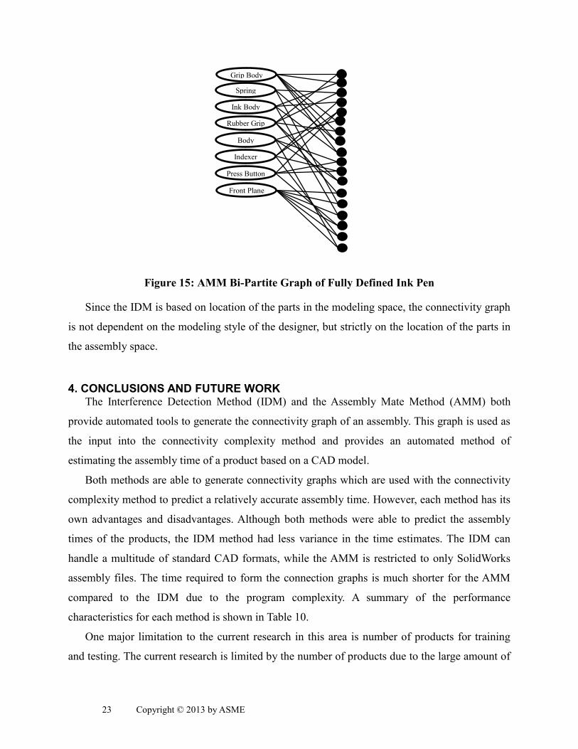
These added relations increase the complexity of the connectivity graph, and therefore also

generate a different complexity vector and bi-partite graph resulting in a different assembly time

estimate (see Figure 15).


Figure 15: AMM Bi-Partite Graph of Fully Defined Ink Pen

Since the IDM is based on location of the parts in the modeling space, the connectivity graph

is not dependent on the modeling style of the designer, but strictly on the location of the parts in

the assembly space.

4. CONCLUSIONS AND FUTURE WORK The Interference Detection Method (IDM) and the Assembly Mate Method (AMM) both

provide automated tools to generate the connectivity graph of an assembly. This graph is used as

the input into the connectivity complexity method and provides an automated method of

estimating the assembly time of a product based on a CAD model.

Both methods are able to generate connectivity graphs which are used with the connectivity

complexity method to predict a relatively accurate assembly time. However, each method has its

own advantages and disadvantages. Although both methods were able to predict the assembly

times of the products, the IDM method had less variance in the time estimates. The IDM can

handle a multitude of standard CAD formats, while the AMM is restricted to only SolidWorks

assembly files. The time required to form the connection graphs is much shorter for the AMM

compared to the IDM due to the program complexity. A summary of the performance

characteristics for each method is shown in Table 10.

One major limitation to the current research in this area is number of products for training

and testing. The current research is limited by the number of products due to the large amount of

Grip Body

Spring

Ink Body

Rubber Grip

Body

Indexer

Press Button

Front Plane


time needed to manually create product models and determine assembly times using the

Boothroyd and Dewhurst assembly time charts. A larger set of product models and assembly

times are needed to further validate the method.

Table 10: Performance Comparison of IDM and AMM

Performance

Metric IDM AMM Section Comments

Accuracy 3.2.

Both methods were relatively accurate,

but statistically AMM had the

advantage.

Modeler

Dependency 3.4.

The IDM is based on part location in

the assembly space as opposed to the

AMM which is based on assembly

mates chosen by the designer. The

assembly mates used may change based

on the designer creating the model.

File Format

Dependency 3.3.

AMM requires SW Assembly Files, but

IDM can use a number of standard

CAD file types

Graph Generation

Time 3.2.

The complexity of the AMM algorithm

is simpler than the IDM resulting in a

much faster graph generation time

Additionally, the construct validity of the method needs to be tested to determine if the

results found from test products with manually estimated assembly times can be used to predict

actual assembly times measured from current manufacturing process. Current collaboration with

a local original equipment manufacturer is underway to validate this work with industry products

and actual assembly times.

Future research directions include significance testing of the complexity vector to determine

if the 29 complexity metrics currently being used are all needed for accurate assembly time


estimation, or if even more metrics may provide better estimates. The current research provides

additional milestones in an ultimate goal of a fully automated assembly time estimation method.

REFERENCES

[1] Sirat M., Tap M., Shaharoun M., and others, 2000, “A Survey Report on Implementation

of Design for Assembly (DFA) in Malaysian Manufacturing Industries,” J. Mek., 1, pp.

60–75.

[2] Khan Z., Boothroyd G., and Knight W., 2008, “Design for Assembly,” Assem. Autom.,

28(3), pp. 200–206.

[3] Boothroyd G., Dewhurst P., and Knight W. A., 2011, Product Design for Manufacture

and Assembly, CRC Press, Boca Raton.

[4] Zha X. F., Lim S. Y. E., and Fok S. C., 1999, “Integrated Knowledge-Based Approach

and System for Product Design for Assembly,” Int. J. Comput. Integr. Manuf., 12(3), pp.

211–237.

[5] Miles B., 1989, “Design for Assembly-A Key Element Within Design for Manufacture,”

Arch. Proc. Inst. Mech. Eng. Part D Transp. Eng. 1984-1988 (vols 198-202), 203(14), pp.

29–38.

[6] Tavakoli M. S., Mariappan J., and Huang J., 2003, “Design for Assembly Versus Design

for Disassembly: A Comparison of Guidelines,” ASME.

[7] Sik Oh J., O’Grady P., and Young R. E., 1995, “A Constraint Network Approach to

Design for Assembly,” IIE Trans., 27(1), pp. 72–80.

[8] Edwards K., 2002, “Towards More Strategic Product Design for Manufacture and

Assembly: Priorities for Concurrent Engineering,” Mater. Des., 23(7), pp. 651–656.

[9] Whitney D. E., and Knovel, 2004, Mechanical Assemblies: Their Design, Manufacture,

and Role in Product Development, Oxford University Press, New York.

[10] Poli C., 2001, Design for Manufacturing, Butterworth Heinemann, Boston.

[11] Maynard H., Stegemerten G. J., and Schwab J., 1948, Methods-Time Measurement,

McGraw-Hill, New York, NY.

[12] Mathieson J., Wallace B., and Summers J. D., “Estimating Assembly Time with

Connective Complexity Metric Based Surrogate Models,” Int. J. Comput. Integr. Manuf.,

on-line(in press).


[13] Owensby E., Shanthakumar A., Rayate V., Namouz E. Z., Summers J. D., and Owensby J.

E., 2011, “Evaluation and Comparison of Two Design for Assembly Methods:

Subjectivity of Information,” ASME International Design Engineering Technical

Conferences and Computers and Information in Engineering Conference, ASME,

Washington, DC, pp. DETC2011–47530.

[14] Owensby J. E., Namouz E. Z., Shanthakumar A., and Summers J. D., 2012,

“Representation: Extracting Mate Complexity from Assembly Models to Automatically

Predict Assembly Times,” ASME International Design Engineering Technical

Conferences and Computers and Information in Engineering Conference, ASME,

Chicago, IL, pp. DETC2012–70995.

[15] Namouz E. Z., and Summers J. D., 2013, “Complexity Connectivity Metrics-Predicting

Assembly Times with Abstract Assembly Models,” Smart Product Engineering, M.

Abramovici, and R. Stark, eds., Springer Berlin Heidelberg, Bochum, Germany, pp. 77–

786.

[16] Mathieson J. L., Wallace B. A., and Summers J. D., 2013, “Assembly time modelling

through connective complexity metrics,” Int. J. Comput. Integr. Manuf., on-line(in press),

pp. 1–13.

[17] Miller M., Mathieson J., Summers J. D., and Mocko G. M., 2012, “Representation:

Structural Complexity of Assemblies to Create Neural Network Based Assembly Time

Estimation Models,” ASME International Design Engineering Technical Conferences and

Computers and Information in Engineering Conference, ASME, Chicago, IL, pp.

DETC2012–71337.

[18] Mathieson J. L., and Summers J. D., 2010, “Complexity Metrics for Directional Node-

Link System Representations: Theory and Applications,” ASME International Design

Engineering Technical Conferences and Computers and Information in Engineering

Conference, ASME, Montreal, Canada, pp. DETC2010–28561.

[19] Francis L., 2001, “Neural Networks Demystified,” Casualty Actuar. Soc. Forum, pp. 253–

320.

[20] Sethi I. K., 1990, “Entropy nets: from decision trees to neural networks,” Proc. IEEE,

78(10), pp. 1605–1613.

[21] Blackard J. a., and Dean D. J., 1999, “Comparative accuracies of artificial neural networks

and discriminant analysis in predicting forest cover types from cartographic variables,”

Comput. Electron. Agric., 24(3), pp. 131–151.

[22] Walpole R. E., Myers R. H., Myers S., and Ye K., 2012, Probability and Statistics for

Engineers and Scientists, Prentice Hall, Englewood Cliffs, NJ.


[23] Montgomery D. C., and Runger G. C., 2010, Applied statistics and probability for

engineers, John Wiley & Sons, Danvers, MA.

comparison of graph generation methods for structural

Documents