comparison of dynamic performance of ann and pid ...ijmtst.com/ncee2017/2.ncee_18.pdfcontrollers for...

5 Volume 3 | Special Issue 02 | March 2017 | ISSN:2455-3778 | www.ijmtst.com/ncee2017.html

Proceedings of National Conference on Emerging Trends in Electrical Technology (NCEE-2017)

Comparison of Dynamic Performance of ANN and PID Controllers for an Interconnected Hydro - Thermal System

V. Anantha Lakshmi1 | J. Rajesh2 | G T Sai Kamal3 | Md.Nadeem4

1Assistant Professor, Department of EEE, Andhra Loyola Institute of Engineering & Technology, Vijayawada, Andhra

Pradesh, India. 2,3,4Department of EEE, Andhra Loyola Institute of Engineering & Technology, Vijayawada, Andhra Pradesh, India.

To Cite this Article V. Anantha Lakshmi, J. Rajesh, G T Sai Kamal and Md.Nadeem, “Comparison of Dynamic Performance of ANN and PID Controllers for an Interconnected Hydro - Thermal System”, International Journal for Modern Trends in Science and Technology, Vol. 03, Special Issue 02, 2017, pp. 05-09.

In this paper a new load frequency controller using the concept of Artificial Neural networks is presented. A

comparison was made, which showed the effectiveness of Artificial Neural Network controller over other

conventional controllers like PID controller. Differences in their steady state intervals have been observed,

when two areas of hydro and thermal stations are interconnected based on back propagation algorithm.

KEYWORDS: Automatic Generation Control, Artificial Neural network (ANN), Back Propagation algorithm,

Area control error

Copyright © 2017 International Journal for Modern Trends in Science and Technology

All rights reserved.

I. INTRODUCTION

The successful operation of interconnected

power systems requires the matching of total

generation with total load demand and associated

system losses. With time, the operating point of a

power system changes, and hence, these systems

may experience deviations in nominal system

frequency and scheduled power exchanges to other

areas, which may yield undesirable effects. In

actual power system operations, the load is

changing continuously and randomly. The ability

of the generation side to track the changing load is

limited due to physical / technical consideration,

causing imbalance between the actual and the

scheduled generation quantities. This action leads

to a frequency variations. The difference between

the actual and the synchronous frequency causes

mal operation of sophisticated equipment like

power converters by producing harmonics.

II. NEED OF LOAD FREQUENCY CONTROL

The active and reactive power demands are

never steady and they continuously changes with

the rising or falling trend of load demand. There is

a change in frequency with the change in load

which causes problems such as:

1. Most AC motors run at speeds that are directly

related to frequency. The speed and induced electro

motive force (e.m.f) may vary because of the change

of frequency of the power circuit.

2 .When operating at frequencies below 49.5 Hz;

some types of steam turbines, certain rotor states

undergo excessive vibration.

ABSTRACT

International Journal for Modern Trends in Science and Technology

Volume: 03, Special Issue No: 02, March 2017

ISSN: 2455-3778

http://www.ijmtst.com

http://www.ijmtst.com/



3. The change in frequency can cause mal

operation of power converters by producing

harmonics.

4. For power stations running in parallel it is

necessary that frequency of the network must

remain constant for synchronization of generators.

III. EXISTING CONTROLLERS AND GAPS

The performance evaluation based on different

conventional controllers (PI & PID) and intelligent

controllers like (Fuzzy, ANN) with different gain

scheduling has been carried out. The fuzzy

controller offers better performance over the

conventional controllers, especially, in complex

and nonlinearities associated system. Among the

various types of load frequency controllers, the

most widely employed is the conventional

proportional integral (PI) controller. The PI

controller is simple for implementation but

generally gives large frequency deviations. The

performance of PI and PID controllers deteriorates

as the complexity of the system increased due to

the nonlinearity and boilers dynamics in the

interconnected power system. In order to keep the

system performance near its optimum, it is

desirable to track the operating conditions and use

updated parameters to compute the control.

Fuzzy technique has been applied to the Load

Frequency Control problems with rather promising

results. The salient feature of these techniques is

that they provide a model-free description of

control systems and do not require model

identification. Whereas fuzzy control technique

also has some limitations of selecting proper

membership functions and defuzzification

problem. Then it has been thought of a controller

which can even work with nonlinearities and can

give fast response. The Artificial Neural Network

came in existence. By training the neurons,

multiplying with weight and applying a suitable

activation function, the output can be obtained.

The ANN controller works better for large power

system or unstructured system.

IV. BIOLOGICAL NEURAL NETWORK

Human brain has over 100 billion

interconnected neurons. Most sophisticated

application have only tiny fraction of that. It can

only be imagined how powerful NN with this

number of interconnected neurons would be.

Neurons use this interconnected network to pass

information‟s with each other using electric and

chemical signals. Although it may seem that

neurons are fully connected, two neurons actually

do not touch each other. They are separated by tiny

gap call synapse. Each neuron process information

and then it can “connect” to as many as 50 000

other neurons to exchange information. If

connection between two neuron is strong enough

(will be explained later) information will be passed

from one neuron to another. On their own, each

neuron is not very bright but put 100 billion of

them together and let them take to each other, then

this system becomes very powerful. A typical

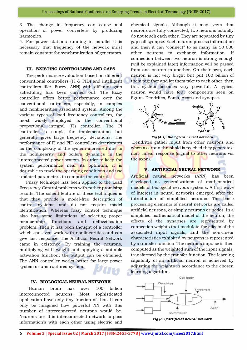
neuron would have four components seen on

figure. Dendrites, Soma, Axon and synapse.

Fig (4.1): Biological neural network

Dendrites gather input from other neurons and

when a certain threshold is reached they generate a

non- linear response (signal to other neurons via

the axon).

V. ARTIFICIAL NEURAL NETWORK

Artificial neural networks (ANN) has been

developed as generalizations of mathematical

models of biological nervous systems. A first wave

of interest in neural networks emerged after the

introduction of simplified neurons. The basic

processing elements of neural networks are called

artificial neurons, or simply neurons or nodes. In a

simplified mathematical model of the neuron, the

effects of the synapses are represented by

connection weights that modulate the effects of the

associated input signals, and the non-linear

characteristics exhibited by neurons is represented

by a transfer function. The neurons impulse is then

computed as the weighted sum of the input signals,

transformed by the transfer function. The learning

capability of an artificial neuron is achieved by

adjusting the weights in accordance to the chosen

learning algorithm.

Fig (5.1):Artificial neural network



A typical artificial neuron and the modelling of a

multi layered neural network are illustrated in

architecture. Referring to the architecture, the

signal flow from inputs nxx ............1 is considered to be

unidirectional, which are indicated by arrows, as

is a neuron output flow )(Y . The neuron output

signal flowY is given by the following relationship:

)()(1

j

n

j

j xwfnetfY

Where jw the weight vector, and the function

is )(netf is referred to as an Activation (transfer)

function. The variable net is defined as a scalar

product of weight and input vectors,

nn

T xwxwxwnet ......11

Where T is the transpose of a matrix, and in the

simplest case, the output value is computed as

xifw

otherwise

T

netfY 1

0{)(

Where is called threshold level; and this type of

node is is called a linear threshold unit.

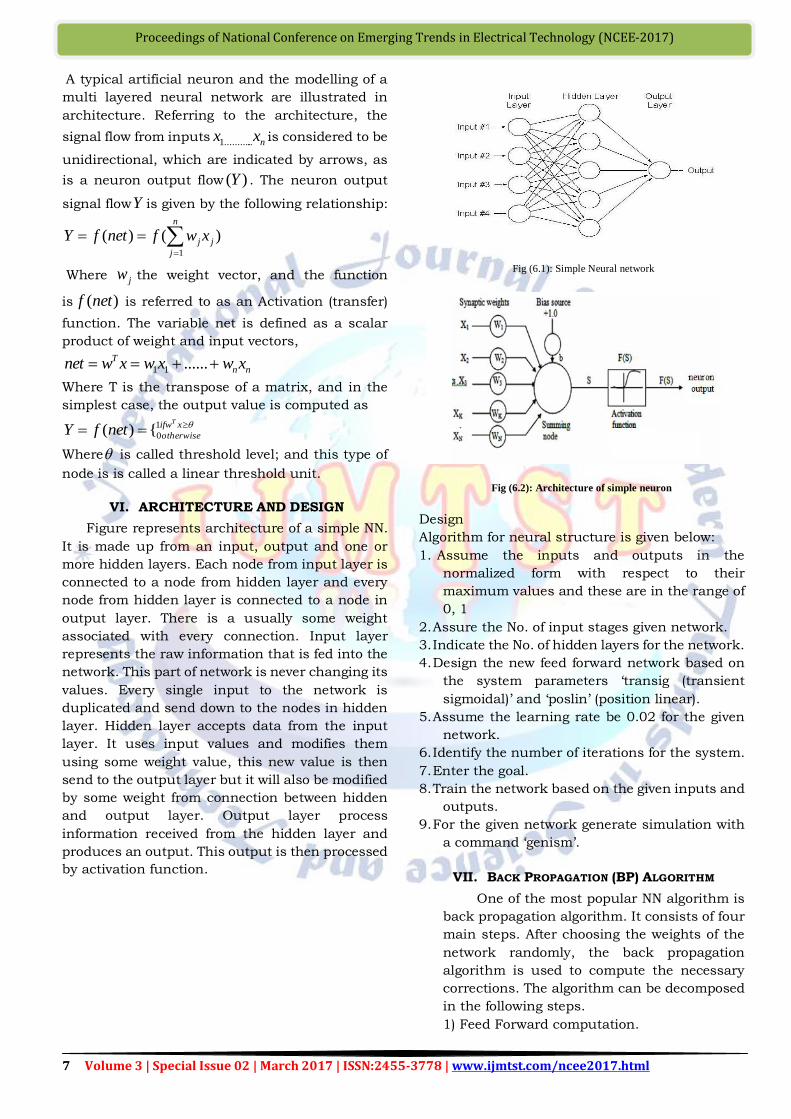
VI. ARCHITECTURE AND DESIGN

Figure represents architecture of a simple NN.

It is made up from an input, output and one or

more hidden layers. Each node from input layer is

connected to a node from hidden layer and every

node from hidden layer is connected to a node in

output layer. There is a usually some weight

associated with every connection. Input layer

represents the raw information that is fed into the

network. This part of network is never changing its

values. Every single input to the network is

duplicated and send down to the nodes in hidden

layer. Hidden layer accepts data from the input

layer. It uses input values and modifies them

using some weight value, this new value is then

send to the output layer but it will also be modified

by some weight from connection between hidden

and output layer. Output layer process

information received from the hidden layer and

produces an output. This output is then processed

by activation function.

Fig (6.1): Simple Neural network

Fig (6.2): Architecture of simple neuron

Design

Algorithm for neural structure is given below:

1. Assume the inputs and outputs in the

normalized form with respect to their

maximum values and these are in the range of

0, 1

2. Assure the No. of input stages given network.

3. Indicate the No. of hidden layers for the network.

4. Design the new feed forward network based on

the system parameters „transig (transient

sigmoidal)‟ and „poslin‟ (position linear).

5. Assume the learning rate be 0.02 for the given

network.

6. Identify the number of iterations for the system.

7. Enter the goal.

8. Train the network based on the given inputs and

outputs.

9. For the given network generate simulation with

a command „genism‟.

VII. BACK PROPAGATION (BP) ALGORITHM

One of the most popular NN algorithm is

back propagation algorithm. It consists of four

main steps. After choosing the weights of the

network randomly, the back propagation

algorithm is used to compute the necessary

corrections. The algorithm can be decomposed

in the following steps.

1) Feed Forward computation.



2) Back propagation to the output layer.

3) Back propagation to the hidden layer.

4) Weight updates.

The updation of weights in back

propagation algorithm is done as follows:

The error signal at the output of neuron jat

iteration n is given by

)()()( nyndne jjj (1)

The instantaneous value of error for neuron j is

)(2

21 ne j . The instantaneous value )(n of total

errors obtained by summing )(2

21 ne j of all

neurons in output layer

)(2/1)(2

nencj

j

(2)

Where c includes all neurons in the output layer.

Average squared error is given by

N

nNavg n

1

1 )( (3)

Where N is total number of patterns in training set.

So minimization of avg is required. So back

propagation algorithm is used to update the

weights. Induced local field )(nv j produced at

input of activation function is given by

)()()(0

nxnwnv i

m

i

jij

(4)

Where m is the number of inputs applied to

neuron to neuron j. So the output is written as

))(()( nvny jjj (5)

The back propagation algorithm applies a

correction )(nwji to weights )(nw ji which is

proportional to partial derivative )(

)(

nw

n

ji

,

which can be written as

)(

)(

)(

)(

)(

)(

)(

)(

)(

)(...

nw

nv

nv

ny

ny

ne

ne

n

nw

n

ji

j

j

j

j

j

jji

(6)

Differentiating the equation(2) with respect to

)(ne j

)()(

)(ne jne

n

j

(7)

Differentiating equation (1) with respect to

1)(

)(

ny

ne

j

j

(8)

Differentiating equation (5) we get

))((1

)(

)(nv jjnv

ny

j

(9)

Differentiating equation (4) with respect

to )(nw ji

)()(

)(nxinw

nv

ji

j

(10)

So using equation(7-10) in equation(6) we get

)())(()( 1

)(

)(nxnvne ijjjnw

n

ji

(11)

The correction applied to is defined by

)(

)()(

nw

n

jiji

nw

(12)

Where is learning rate parameter. It is seen

that the Area Control Error (ACE) and rate of

change of ACE are considered as inputs in the

input layer and is considered as output in the

output layer.

Fig (8.1): MATLAB/SIMULINK Implementation of logic

Fig (8.2): Block diagram of interconnected hydro-thermal

system

Fig(8.3):Simulink model of Hydro-Thermal system with

PID controller



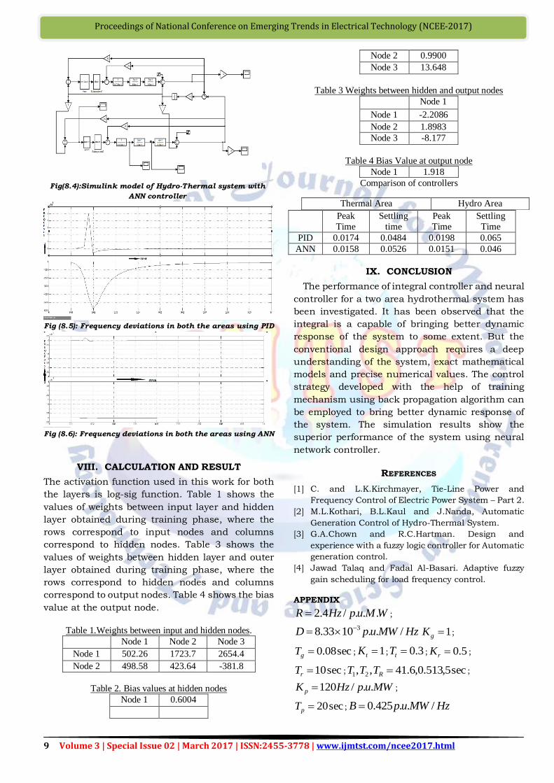
Fig(8.4):Simulink model of Hydro-Thermal system with

ANN controller

Fig (8.5): Frequency deviations in both the areas using PID

Fig (8.6): Frequency deviations in both the areas using ANN

VIII. CALCULATION AND RESULT

The activation function used in this work for both

the layers is log-sig function. Table 1 shows the

values of weights between input layer and hidden

layer obtained during training phase, where the

rows correspond to input nodes and columns

correspond to hidden nodes. Table 3 shows the

values of weights between hidden layer and outer

layer obtained during training phase, where the

rows correspond to hidden nodes and columns

correspond to output nodes. Table 4 shows the bias

value at the output node.

Table 1.Weights between input and hidden nodes.

Node 1 Node 2 Node 3

Node 1 502.26 1723.7 2654.4

Node 2 498.58 423.64 -381.8

Table 2. Bias values at hidden nodes

Node 1 0.6004

Node 2 0.9900

Node 3 13.648

Table 3 Weights between hidden and output nodes

Node 1

Node 1 -2.2086

Node 2 1.8983

Node 3 -8.177

Table 4 Bias Value at output node

Node 1 1.918

Comparison of controllers

Peak

Time

Settling

time

Peak

Time

Settling

Time

PID 0.0174 0.0484 0.0198 0.065

ANN 0.0158 0.0526 0.0151 0.046

IX. CONCLUSION

The performance of integral controller and neural

controller for a two area hydrothermal system has

been investigated. It has been observed that the

integral is a capable of bringing better dynamic

response of the system to some extent. But the

conventional design approach requires a deep

understanding of the system, exact mathematical

models and precise numerical values. The control

strategy developed with the help of training

mechanism using back propagation algorithm can

be employed to bring better dynamic response of

the system. The simulation results show the

superior performance of the system using neural

network controller.

REFERENCES

[1] C. and L.K.Kirchmayer, Tie-Line Power and

Frequency Control of Electric Power System – Part 2.

[2] M.L.Kothari, B.L.Kaul and J.Nanda, Automatic

Generation Control of Hydro-Thermal System.

[3] G.A.Chown and R.C.Hartman. Design and

experience with a fuzzy logic controller for Automatic

generation control.

[4] Jawad Talaq and Fadal Al-Basari. Adaptive fuzzy

gain scheduling for load frequency control.

APPENDIX

WMupHzR .../4.2 ;

HzMWupD /..1033.8 3 1gK ;

sec08.0gT ; 1tK ; 3.0tT ; 5.0rK ;

sec10rT ; sec5,513.0,6.41,, 21 RTTT ;

MWupHzK p ../120 ;

sec20pT ; HzMWupB /..425.0

Thermal Area Hydro Area

comparison of dynamic performance of ann and pid ...ijmtst.com/ncee2017/2.ncee_18.pdfcontrollers for...

Documents