COMPARISON AND EVALUATION OF AIR POLLUTION DISPERSION MODELS AERMOD AND ISCST-3 DURING PRE-MONSOON MONTH OVER RANCHI

RAHUL BOADH1*, SATYANARAYANA A N V2 AND RAMA KRISHNA T V B P S3

1Department of Mathematics, Madanapalle Institute of Technology and Science, Madanapalle-517325, India2Center for Oceans, Rivers, Atmosphere and Land Sciences, Indian Institute of Technology Kharagpur,

Kharagpur-721302, India3CSIR-NEERI Hyderabad Zonal Laboratory, IICT Campus, Uppal Road, Hyderabad-500007, India

(Received 17 June, 2016; accepted 18 January, 2017)

Key words: Dispersion, Atmospheric boundary layer, AERMOD, ISCST-3

INTRODUCTIONAir pollution has been with us since the first fire was lit, although different aspects have been important at different times. While many of us would consider air pollution to be an issue that the modern world has resolved to a greater extent, it still appears to have considerable influence on the global environment. In many countries with ambitious economic growth targets the acceptable levels of air pollution have been transgressed, resulting in an urban skyline characterized by smog and dust clouds. In several Indian cities with population of over a million, air pollution levels exceed World Health Organization standards. According to World Health Report (2002), it has been estimated that in India alone about 500,000 premature deaths are caused each year by indoor air pollution, mainly affecting mothers and their children under 5 years of age. Serious

ABSTRACT

Accurate representation of air pollutant dispersion is essential for environmental management and planning purposes. In the present study, two state-of-art air pollution dispersion models, namely AERMOD and ISCST-3 are implemented during the pre-monsoon period of 2010 at Ranchi. AERMOD model is equipped with comprehensive atmospheric boundary layer processes and the other model is based on Gaussian Plume Dispersion concepts only. The purpose of the study is to understand the dispersion of air pollutants such as SO2, NOX and PM10 at Ranchi and additionally the model inter-comparison. The AERMOD model derived boundary layer parameters are validated with the available micro-meteorological tower based in-site measurements and upper air measurements at Ranchi during 1-7 April 2010. The results indicate that boundary layer process which influence the dispersion of the pollutants are better represented in AERMOD model. Spatial distribution of the above-mentioned air pollutants is estimated using AERMOD and ISCST-3 over Ranchi. Dispersion patterns are compared with the windroses. Validation of the concentration distribution of air pollutants of these models are done and found that AERMOD is performing better than ISCST-3. This study advocates that for all air pollution assessment studies it is better to use AERMOD to that of ISCST-3.

Jr. of Industrial Pollution Control 33(1)(2017) pp 674-685www.icontrolpollution.comResearch

*Corresponding author's email: rahulboadhmsc26@gmail.com

respiratory disease-related problems have been identified for both indoor and outdoor pollution in major cities of several countries. Many atmospheric factors influence the way air pollution is dispersed, including wind direction and wind speed, type of terrain and heating effects. Boadh et al. (2016) studied and concluded that to had better understand how atmosphere processes can affect ground level pollution, atmospheric conditions can be described simply as either stable or unstable, where the stability is determined by wind (which stirs the air) and heating effects (which cause convection currents). Atmospheric stability affects pollution released from ground level and elevated sources differently. Boadh et al. (2014) studied the dispersion of NOX during summer over Ranchi and concluded that observed that the model show distinct variations of spatial concentration from day to day. Some observational

675

air quality studies over Visakhapatnam provided an overview of air pollution causes, sources, pollutants and its adverse effects on environment (Srinivas and Purushotham 2013, Kumar and Durupa 2013).

Air dispersion modeling is the mathematical summation of how air pollutants disperse in the ambient atmosphere. Boadh et al. (2015) also used WRF-WERMOD coupled modeling system for finding the NOX concentration over Vishakhapatnam. It is performed with computer programs that solve the mathematical equations and algorithms which simulate the pollutant dispersion. Plethora of air pollution dispersion models are available for varied applications. Keeping in view of the importance of air pollution and its hazardous implications, in the present study an attempt has been made to study the dispersion of various air pollutants over Ranchi using an industry emission inventory. For this purpose, two important dispersion models namely AERMOD and ISCST-3 are implemented.

STUDY REGIONAnnaba Ranchi is the capital of the newly formed state of Jharkhand. Ranchi is located on the eastern parts of the Indian sub-continent seen in (Fig. 1). The summer is warm but bearable with average high temperature during summer is around 37.2°C. The winter in turn is quiet pleasant with average temperature dipping up to 10.3°C. Ranchi city is located between 23018’43.54” N to 23022’39.35” N and 85016’47.88” E to 85021’38.71” E, 274.5 and 652.70 meters above sea level. Average annual precipitation is 2078 millimeters with 34% of the total rainfall occurring in the month of July. Rainfall averages 7.20 cm monthly. 28% of Ranchi is covered by forest. The climate of Ranchi follows a typical seasonal monsoon weather pattern.

Fig. 1 Study area (Ranchi city map), taken from Google

Earth.

The peak temperatures are usually reached in April/

May and can be as high as 35.5°C before monsoons. According to Census of India 2001, it has a population of 40, 51,444. Ranchi, the city economic development, has been under stress due to increasing urbanization and industrialization. Ranchi is one of the industrial colonies of Jharkhand. Traffic flow is Ranchi is also high in India. Vehicular population in Ranchi for year 2010 was about the 9 lakh’s vehicles plying on city roads, 80% are two wheelers while the rest fall in the category of heavy vehicles, three wheelers and four- wheelers. In addition to this are the vehicles used by the floating population.

DATAThe emission and primary pollutants namely SO2, NOX and PM10 emitted from different industrial sources and their source characteristics, meteorological and ambient air quality data (Ranchi 2010) are described in this section.

Emission data

There are about 28 industrial sources located in an industry at Ranchi that are considered in the present study. All of them are considered as the point sources as they are stacks releasing the affluent into the atmosphere. The industrial stacks that are connected to process and operation (confined sources) are considered as elevated point sources for computing the emission rate/source strength of these sources such as stack height, internal diameter, exit velocity and exit temperature are considered along with emission (in gs-1) of SO2, NOX and PM10. The location (X, Y) on the Cartesian grid of these point sources is also taken. The characteristics of the elevated point sources used in the simulations are given in Table 1. Cartesian grid locations of stack are shown in the (Fig. 2).

Fig. 2 Stack location on Cartesian grid used both AERMOD and ISCST-3 model.

Used the same stack locations in AERMOD and ISCST-3 show location and with the centre point at 10000-10000 m at x axis and y axis and origin (0, 0) is it SW corner or lowest left corner of the given graphs. A grid spacing of 500 m is used over the total grid area of 20 km × 20 km i.e. Ranchi station and region

BOADH ET AL.

676COMPARISON AND EVALUATION OF AIR POLLUTION DISPERSION MODELS

AERMOD AND ISCST-3

for predicting the GLCS of air pollutants SO2, NOX and PM10.

Meteorological data

The meteorological data for 7 days in April (1-7 April 2010) represent pre-monsoon season is used in the present study. The meteorological data comprises the hourly wind speed, wind direction, temperature, cloud cover and solar radiation. Sensible heat Flux and friction velocity data over the Ranchi during study period is also considered. Upper air observations during the study period are obtained from web-link

of University of Wyoming http://weather.uwyo.edu/upperair/. A fair estimate of the dispersion of pollutants in the atmosphere is possible based on the frequency distribution of wind direction as well as wind speed (Manju et al., 2002). (Fig. 3) illustrates the wind roses for the study period in 1-7 April 2010. Maximum wind direction in 1-7 April 2010 WSW, W, WWN, NW, and NNW direction and calms of wind are 7.86% in 1-7 April 2010. It is seen that the wind direction is varies from WNS and NW during the study period 1-7 April.

S. No Stack name Stack height(m) diameter (m) Velocity (m/s) Temp. (K) SO2 (g/s) PM (g/s) NOX (g/s)

1 F3 Main Furnace 11.5 0.4 4.2951105 381 0.00464 0.0194 0.00842 F3 Zinc Bath 11.5 0.4 2.7014996 445 0.00364 0.0193 0.00393 F3 Lead Bath 11.5 0.4 2.5488394 405 0.004 0.0163 0.00424 MS1 Zinc Bath 11.75 0.4 3.2417847 418 0.00435 0.0136 0.00645 MS1 Lead Bath 14.5 0.4 2.7031769 381 0.00372 0.0162 0.00536 MS3 Zinc Bath 15.68 0.4 3.1704344 418 0.00568 0.0361 0.01367 MS3 Lead Bath 15.68 0.4 4.599622 438 0.00432 0.013 0.0059

8 New PHTF Heater 15 0.7 5.0618084 352 0.03297 0.1896 0.0593

9 SSPH TF Heater 10.8 0.254 5.0060351 388 0.00234 0.0162 0.003310 Le-Four Zinc Bath 15 0.483 3.7839936 353 0.00878 0.0257 0.014

11 Le-Four Lead Bath 15 0.483 4.2527668 405 0.01261 0.0258 0.0212

12 Le-Four MF 15 0.483 5.5131207 537 0.00896 0.0252 0.0162

13 Le-Four TF Heater 15 0.635 3.4591314 315 0.02072 0.059 0.0466

14 DSW Main furnace 15 0.53 6.2161139 557 0.011 0.0763 0.0176

15 DSW Lead Bath 15 0.3 3.5580312 335 0.00492 0.021 0.005416 DSW Zinc Bath 15 0.483 3.8744326 334 0.00823 0.0374 0.011417 F4 Main Furnace 13.5 0.4 4.6119046 469 0.00589 0.0188 0.007718 F4 Zinc Bath 13.5 0.4 2.7915818 347 0.00361 0.0102 0.004819 F4 Lead Bath 13.5 0.4 2.0438806 340 0.0036 0.02 0.006320 Aqua t Heater 13 0.3 1.4406019 324 0.00169 0.0058 0.0036

21 1000 KVA DG sno.8 10.2 0.3 14.947848 639 0.00936 0.064 0.0222

22 1000 KV no.8(L) 10.2 0.3 15.757207 639 0.02077 0.0675 0.0234

23 1000 KVAD no.9 ® 10.2 0.3 16.118254 632 0.02363 0.0693 0.0258

24 1000 KVDno.2(L) 10.2 0.3 16.118254 632 0.01987 0.0623 0.022

25 1010 KVA DGno.12 9.5 0.35 8.2919741 429 0.01883 0.0676 0.0205

26 1010 KVA DG no.13 9.5 0.35 8.2733337 419 0.02433 0.0588 0.0328

27 1010 KVA DGno.10 9.5 0.3 11.106124 423 0.02322 0.0619 0.0354

28 1010 KVA DG11 9.5 0.3 11.435045 428 0.02138 0.0596 0.0259

Table 1. Stack location over an Industry at Ranchi

677

Dispersion model

The detail of the dispersion models (ISCST-3 & AERMOD) that are implemented in present section.

ISCST-3 model

The ISCST model is the most widely used model for ambient air quality applications. The description of ISCST model is given below:

ISCST-3 model is developed by US Environmental Protection Agency (EPA) for computing the ground level concentrations of the pollutant. This model has the capability to handle polar or Cartesians co-ordinates, simulates point, area, and volume sources, considers wet and dry deposition, makes terrain adjustments, and considers building downwash. The details of the model are given below briefly for completeness of the presentation.

The ISCST-3 model for continuous elevated point sources use the steady–state Gaussian Plume equation given by

2

2exp[ ]2 2.π σ σ σ

= −y z y

QKVD yCu

(1)

Where Q is the source strength or emission rate of pollutant (gs-1), where u is the mean wind speed (ms-1), y is the cross wind distance (m), σy and σz are the dispersion parameters (m) in the horizontal and vertical directions, respectively, K is the scaling coefficient to convert calculated concentrations to desired units, V is the term for vertical distribution of Gaussian plume and S is the decay term accounting for the pollutant removal by physical or chemical process. The expressions for V in eq. (1) is given by:

{ }

2 2

2 2

22 2 231 2 4

2 2 2 21

exp 0.5 exp 0.5

exp 0.5 exp[ 0.5 exp[ 0.5 exp[ 0.5

σ σ

σ σ σ σ

∞

=

− + = − + − +

− + − + − + −

∑

r e r e

i

Z h Z hV

HH H H

Where he = hs+ h∆

Fig. 3 Wind roses for 1-7April 2010 over Ranchi.

BOADH ET AL.

678

1 r i e 2 r i e

3 r i e 4 r i e

H = z + (2iz -h ); H = z + (2iz +h ); H = z - (2iz +h ); and H = z - (2iz -h )

in which zr is the receptor height above ground or flag pole (m), he is the effective stack height (m), hs is the effective stack height (m), hs is the physical stack height (m), ∆h is the plume rise (m), zi is the mixing height (m).

Eq. (2) is the vertical term without dry deposition. The infant series terms in Eq. (2) accounts for the effects of the restriction on vertical plume growth at the top of the mixing layer. The method of image sources is used to account for multiple reflections of the plume from the ground surface and the top of the mixed layer. If the effective stack height (he) exceeds the mixing height, the plume is assumed to fully penetrate the elevated inversions and the ground level concentrations are set to zero. The vertical term Eq. (2) changes the form of the vertical concentration distribution from Gaussian to rectangular (i.e. a uniform concentration distribution within the surface mixing layer) along downwind distances.

The expression for D in eq. (1) is given by:

{exp

1 0 0s

xu

forD f orϕ

ϕ ϕ == >

Where Ψ is the decay coefficients (s-1) (a value of zero means decay is not considered), x is the downwind distance (m). If T½ is the half-life in seconds then Ψ can be obtained by 1

20.693 /Tψ =

The ISCST-3 model employs Briggs formulae to compute plume rise and Psiquill–Gifford curves for parameterizing the horizontal and vertical distribution parameters and it includes buoyancy –induced dispersion. This model has an option to use rural or urban backgrounds. Wind profile law is used to estimate the wind speed at stack height (ISC-3).

AERMODA committee, AERMIC (the American Meteorological Society/Environmental Protection Agency Regulatory Model Improvement Committee), was formed to introduce state of the art modeling concepts into the EPA’s local-scale air quality models. AERMOD model basically depend on conservation low. Conservation law is the following: -

2

2 2

2( , , ) .exp .2 . 2.

( (exp exp

2. 2.

π σ σ σ

σ σ

= −

− +

− + −

y z

eff eff

z z

Q yC X Y Zu y

z H z H

Where c(x, y, z) = concentration at x, y, z.

u = wind speed (downwind, m/sec).

σy and σz= S.D. of concentration in y and x.

Q= emission (g/s) and 𝐻eff= effective stack height.

And one of the important conservation equations is following:-

1 2 3. .. 2. . 2σ π σ π

+ +=

z z

Q f g g gCu

Where

f = crosswind dispersion parameter = 2

2exp[ ]2.

yyσ

−

g = vertical dispersion parameter =g1 + g2 + g3

g1= vertical dispersion with no reflection =2

2

(z H)exp[ ]2. zσ−

−

g2= vertical dispersion due to reflection from the

ground = 2

2

(z H)exp[ ]2. zσ−

−

g3= vertical dispersion due to reflection from inversion led aloft =

2 2

2 21

2 2

2 2

(z H) ( 2 ){exp[ ] exp[ ]2. 2.

( 2 ) ( 2 )exp[ ] exp[ ]}2. 2.

σ σ

σ σ

∞

−

− + +− + +

+ − − +− + −

∑ iz z

z z

z H ML

z H ML z H ML

C = Concentration of emissions (g/𝑚3), at any receptor located at:-

x = Meter downwind from the emission source point.

y = Meter crosswind from the emission source point.

z = Meters above ground level.

Q = Source pollutant emission rate, g/s.

u = Horizontal wind velocity along the plume centerline, m/s.

σz= Vertical standard deviation of the emission distribution, m.

σy= Horizontal standard deviation of the emission distribution, m.

H = Emission plume centerline above ground level, m.

L = Distance from ground level to bottom of the inversion, m.

The sum of the four exponential terms in 𝑔3 converge quite rapidly, for most cases, the summation of the series with m=1, m=2 and m=3 will provide an adequate evaluation of the series. It should be noted that 𝜎z and 𝜎y are functions of the downwind distance to the receptor. The model is applicable to primary pollutants and continuous releases of toxic and hazardous waste pollutants. Chemical

COMPARISON AND EVALUATION OF AIR POLLUTION DISPERSION MODELS AERMOD AND ISCST-3

679

transformation is treated by simple exponential decay. ISCST-3 and AERMOD will be used to assess for assessment of air pollutants dispersion in the present study.

RESULTS AND DISCUSSIONThe ground level concentration (GLCs) of the pollutants SO2, NOX and PM10 due to an industrial complex in Ranchi were computed using two air pollution dispersion models AERMOD and ISCST-3 models. The ISCST-3 model was run with readily available meteorological data monitored on 32 meter tower. AERMOD used the boundary layer parameter (surface friction velocity, surface sensible heat flux, Monin-Obukhov length and inversion – mixing height) determined using the flux profile relationship apart from readily available meteorological data. Both the models used the emission data as describe in chapter three. The comparison of computed and observed boundary layer parameter, the GLCs of pollutants computed using AERMOD and ISCST-3 on 24 hourly and 1 hourly average basis and validation of the models concentrations with observed concentrations are presented in this section.

Validation of computed boundary layer parameters

The boundary layer parameter computed using the flux profile relationship which will be given as input to AERMOD are compared with observed parameter monitored using sonic anemometer. Eddy co-variance technique was used for calculating surface friction velocity and surface sensible heat flux.

(Fig. 4) illustrates the validation of diurnal variation of observed/computed and model simulation of

friction velocity using AERMOD during the period 1-7 April 2010. The range of predicted friction velocity 0.01 to 0.95 ms-1 and the range of observed friction velocity is from 0.01 to 0.85 ms-1 and is noticed during the period of the analyzed data. The modeled u* values show slight over-prediction during day time and slight underproduction during night time hours compared to observed values. The modeled and observed u* values show similar trend during entire period expect on 3rd and 4th day. The variation is very high in observed friction velocity in 4th April but in predicted friction velocity variation in 3rd April. Both the compute and predicted values suggests moderate to strong mechanical turbulence during day time and weak turbulence during night time for the whole weak expect on 3rd and 7th April 2010. Friction velocity variation is proportional to the wind speed. It is expected that the higher the wind speed the more is the friction velocity. It varies from 0.01 to 0.85 m/s during the period of the analyzed data. Higher friction velocity is noticed on 6th April.

The comparison of modeled and observed sensible heat flux for the period of 1-7 April 2010 is given in (Fig. 5). Observations revealed well defined and anticipated diurnal variability of sensible heat flux during a drier atmosphere is seen in all the days. In the first three days (1st to 3rd April) the maximum flux of around 250 W m-2 is noticed whereas the rest of the four days higher magnitude of flux is seen with a maximum of around 315 W m-2 especially on 4th and 6th April at the site. It is noted that the computed values are form to be in close argument with the observed values in general. However, the computed values show over-prediction of maximum sensible

Fig. 4 Comparison of diurnal variation of predicted and observed friction velocity.

Fig. 5 Comparison of diurnal variation of predicted and observed sensible heat flux.

BOADH ET AL.

680

heat flux around noon on 1st and 3rd day. The range of computed and sensible heat flux in day time 62 Wm-2 to 376.7 Wm-2 and sensible heat flux varies in night time -29.2 Wm-2 to 6 Wm-2.

Observed sensible heat flux day time variation varies 26 Wm-2 to 315 Wm-2 and night time variation is -32.7117 Wm-2 to 6 Wm-2 Both the compute and predicted values suggests moderate to strong turbulence during day time and weak turbulence during night time for the whole weak expect on 3rd and 7th April 2010 as observed in the case of u*.

Comparison of ground level concentrations (GLCs) of pollutants

The GLCs of pollutants SO2, NOX and PM10 were

predicted using AERMOD and ISCST-3 models. The ISCSt-3 model was run with readily available meteorological data monitored on 32 meter tower. AERMOD used the boundary layer parameter (surface friction velocity, surface sensible heat flux, Monin-Obukhov length and inversion –mixing height) determined using the flux profile relationship apart from readily available meteorological data. Both the models used the emission data as describe in chapter three. The concentration were computed over an area of 20 km × 20 km with the industrial area under consideration at the center of the region the total area is divided into 1681 grid which each grid having a distance of 500 meter. The results are

Fig. 6 Spatial distribution of SO2 (a & b: Top Panel), NOX (c & d: Middle Panel) and PM10 (e & f: Bottom Panel) concentrations obtained using dispersion models AERMOD and ISCST-3 over Ranchi on 3 April 2010.

Fig. 7 Spatial distribution of SO2 (a & b: Top Panel), NOX (c & d: Middle Panel) and PM10 (e & f: Bottom Panel) concentrations obtained using dispersion models AERMOD and ISCST-3 over Ranchi on 5 April 2010.

COMPARISON AND EVALUATION OF AIR POLLUTION DISPERSION MODELS AERMOD AND ISCST-3

681

presented in the form of 24 hourly concentrations and 1 hourly concentration in the following section.

Comparison of 24 hourly GLCs

The GLCs of SO2, NOX and PM10 of 24 hourly average bases are computed using AERMOD and ISCST-3 for 3rd and 5th April 2010. These three days were chosen based on the meteorological features. The incremental GLCs SO2, NOX and PM10 computed using AERMOD due to the emission from industrial area are showing (Fig. 6a, 6c, and 6e) and (Fig. 7a, 7c, and 7e), receptively for days 3rd and 5th April 2010. The incremental GLCs SO2, NOX and PM10 computed using ISCST-3 due to the emission from industrial area is showing (Fig. 6b, 6d, and 6e) and (Fig. 7b, 7d, and 7e), receptively for days 3rd and 5th April 2010. In day 3rd the maximum incremental GLCs of SO2 (Fig. 6a and 6b), NOX (Fig. 6c and 6d) and PM10 (Fig. 6e and 6f) are found N and NW direction from the industrial location. However on day 5th the maximum incremental GLCs of SO2 (Fig. 7a and 7b), NOX (Fig. 7c and 7d) and PM10 (Fig. 7e and 7f) are found to occur near the industrial location. Both the models reveal significant day to day variability in the dispersion of the air pollutants as given in the previous sections. It is also observed that ISCST-3 slightly over-prediction compared to AERMOD.

The 24 hourly concentrations of SO2, NOX and PM10 computed using AERMOD and ISCST-3 models are compared and given in Tables 2, 3 and 4 respectively. The comparison of SO2 concentrations computed using AERMOD and ISCST-3 models show that ISCST-3 model over predicts the concentration compared to AERMOD predicted values in all days expect on 7th day as given in Table 2. The GLCs of SO2 predicted by AERMOD are varying from 0.36035 µgm-3 (on day 3) to 1.18344 µgm-3 (on day 2) whereas the GLCs of SO2 predicted by ISCST-3 are ranging from 0.77428 µgm-3 (on day 3) to 1.46749 µgm-3 (on day 4).

Table 3 gives the comparison of NOX concentrations computed using AERMOD and ISCST- 3 models. The comparison shows that ISCST-3 model over predicts the concentration compared to AERMOD predicted values in all days expect on 7th day. The GLCs of NOX predicted by AERMOD are varying from 0.52652 µgm-3 (on day 3) to 1.62368 ug/m3 (on day 2) whereas the GLCs of NOX predicted by ISCST-3 are ranging from 1.20223 µgm-3 (on day 3) to 2.03284 µgm-3 (on day 4).

The comparison of PM10 concentrations computed using AERMOD and ISCST-3 models is given in Table 4 it can be seen that the ISCST-3 model over predicts the concentration compared to AERMOD predicted values in all days expect on 7th day.

Days Concentration of SO2 (ug/m3) over Ranchi April 1-7 2010

AERMOD ISCST-31 0.81675 1.424502 1.18344 1.343683 0.36035 0.774284 0.42967 1.467495 0.61923 1.198226 0.39033 0.789607 0.91857 0.81380

Table 2. SO2 24 hourly concentration

Days Concentration of NOx (ug/m3) over Ranchi April 1-7 2010

AERMOD ISCST-31 1.09721 1.862732 1.62368 1.760653 0.52652 1.202234 0.60175 2.030845 0.95944 1.734996 0.66034 1.385897 1.39531 1.26912

Table 3. NOX 24 hourly concentration

Days Concentration of PM10(ug/m3) over Ranchi April 1-7 2010

AERMOD ISCST-31 2.63581 7.244302 3.90334 6.794203 1.28931 4.421694 1.44636 6.960855 2.90422 6.621636 1.56851 4.583517 4.17165 4.07512

Table 4. PM10 24 hourly concentration

The GLCs of PM10 predicted by AERMOD are varying from 1.28931 µgm-3 (on day 3) to 4.17165 µgm-

3 (on day 7) whereas the GLCs of PM10 predicted by ISCST-3 are ranging from 4.07512 µgm-3 (on day 7) to 7.24430 µgm-3 (on day 1). From these results it is observed that ISCST-3 over predicted compare to AERMOD in general. This may be due to the fact that AERMOD uses the bi Gaussian distribution during the day time convective conditions.

Comparison of hourly GLCs

The GLCs of SO2, NOX and PM10on hourly average bases are computed using AERMOD and ISCST-3 for 7April 2010. The diurnal variation of wind speed and mixing for day 7 is show in (Fig. 8), the hourly SO2 concentration predicted by AERMOD and ISCST-3 are presented in (Fig. 9).

The maximum SO2 concentration predicted by AERMOD is 11.9 µgm-3 and by ISCST-3 is 8.4 µgm-3 found to be occurring during 9-10 am. The

BOADH ET AL.

682

SO2 concentration predicted by both the models (AERMOD and ISCST-3) show similar behavior. The models predicted concentrations are found to be high when wind speed and mixing height are low (Fig. 8). (Fig. 10) illustrates the hourly NOX concentration predicted by AERMOD and ISCST-3. The maximum NOX concentration predicted by AERMOD is 15 µgm-

3 and by ISCST-3 is 11.5 µgm-3 found to be occurring during 9-10 am. Secondary maximum of 8.5 µgm-3 predicted by AERMOD is observed at 8 am whereas ISCST-3 does not show any secondary maximum.

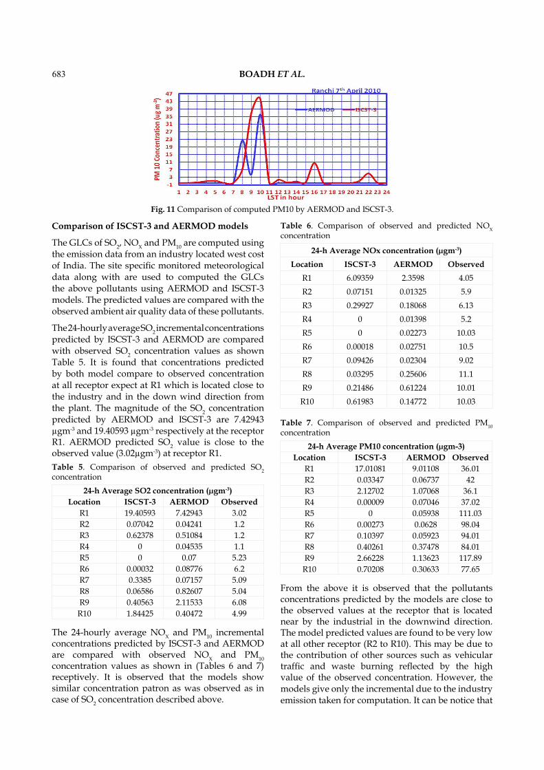
The maximum PM10 concentration predicted by AERMOD is 36 µgm-3 and by ISCST-3 is 44 µgm-

3 found to be occurring during 9-10 am as show in (Fig. 11). Secondary maximum of 23 µgm-3 predicted by AERMOD is observed at 8 am whereas ISCST-3 does not show any secondary maximum. The models

predicted concentrations are found to be high when wind speed and mixing height are low (Fig. 8). The higher concentrations of the pollutants are found to occur during the morning hours (8 to 10 am). This may be due to the fumigation inversion condition in these hours. It is also observed that ISCST-3 simulated higher PM10 concentration than AERMOD. Interestingly AERMOD simulations reveal higher concentrations of gases pollutants than ISCST-3. The differences of the concentration predicted by the AERMOD and ISCST-3 are due to representation of atmospheric turbulence differently. ISCST-3 estimate the stability classification as a function of wind speed, solar radiation (day time), and clout cover (night time) whereas AERMOD classify the atmospheric stability as function of Monin-Obukhov length.

Fig. 8 Diurnal variations of mixing height and wind speed.

Fig. 9 Comparison of computed SO2 by AERMOD and ISCST-3.

Fig. 10 Comparison of computed NOX by AERMOD and ISCST.

COMPARISON AND EVALUATION OF AIR POLLUTION DISPERSION MODELS AERMOD AND ISCST-3

683

Comparison of ISCST-3 and AERMOD models

The GLCs of SO2, NOX and PM10 are computed using the emission data from an industry located west cost of India. The site specific monitored meteorological data along with are used to computed the GLCs the above pollutants using AERMOD and ISCST-3 models. The predicted values are compared with the observed ambient air quality data of these pollutants.

The 24-hourly average SO2 incremental concentrations predicted by ISCST-3 and AERMOD are compared with observed SO2 concentration values as shown Table 5. It is found that concentrations predicted by both model compare to observed concentration at all receptor expect at R1 which is located close to the industry and in the down wind direction from the plant. The magnitude of the SO2 concentration predicted by AERMOD and ISCST-3 are 7.42943 µgm-3 and 19.40593 µgm-3 respectively at the receptor R1. AERMOD predicted SO2 value is close to the observed value (3.02µgm-3) at receptor R1.

24-h Average SO2 concentration (µgm-3)Location ISCST-3 AERMOD Observed

R1 19.40593 7.42943 3.02R2 0.07042 0.04241 1.2R3 0.62378 0.51084 1.2R4 0 0.04535 1.1R5 0 0.07 5.23R6 0.00032 0.08776 6.2R7 0.3385 0.07157 5.09R8 0.06586 0.82607 5.04R9 0.40563 2.11533 6.08R10 1.84425 0.40472 4.99

Table 5. Comparison of observed and predicted SO2 concentration

The 24-hourly average NOX and PM10 incremental concentrations predicted by ISCST-3 and AERMOD are compared with observed NOX and PM10 concentration values as shown in (Tables 6 and 7) receptively. It is observed that the models show similar concentration patron as was observed as in case of SO2 concentration described above.

24-h Average NOx concentration (µgm-3)Location ISCST-3 AERMOD Observed

R1 6.09359 2.3598 4.05R2 0.07151 0.01325 5.9R3 0.29927 0.18068 6.13R4 0 0.01398 5.2R5 0 0.02273 10.03R6 0.00018 0.02751 10.5R7 0.09426 0.02304 9.02R8 0.03295 0.25606 11.1R9 0.21486 0.61224 10.01R10 0.61983 0.14772 10.03

Table 6. Comparison of observed and predicted NOX concentration

24-h Average PM10 concentration (µgm-3)Location ISCST-3 AERMOD Observed

R1 17.01081 9.01108 36.01R2 0.03347 0.06737 42R3 2.12702 1.07068 36.1R4 0.00009 0.07046 37.02R5 0 0.05938 111.03R6 0.00273 0.0628 98.04R7 0.10397 0.05923 94.01R8 0.40261 0.37478 84.01R9 2.66228 1.13623 117.89R10 0.70208 0.30633 77.65

Table 7. Comparison of observed and predicted PM10 concentration

From the above it is observed that the pollutants concentrations predicted by the models are close to the observed values at the receptor that is located near by the industrial in the downwind direction. The model predicted values are found to be very low at all other receptor (R2 to R10). This may be due to the contribution of other sources such as vehicular traffic and waste burning reflected by the high value of the observed concentration. However, the models give only the incremental due to the industry emission taken for computation. It can be notice that

Fig. 11 Comparison of computed PM10 by AERMOD and ISCST-3.

BOADH ET AL.

684

one cannot make any significant conclusion on the merits or demerits of AERMOD and ISCST-3 from the above validation study and can remain to be seen the behavior of these models by applying them at different sites for different sources.

CONCLUSIONSIn the present study, an attempt has been made to understand the dispersion of air pollution by employing two dispersion models namely AERMOD and ISCST-3 over Ranchi, an industrial city and capital of Jharkhand state during pre-monsoon period of 2010. In general, both the models are based on Gaussian Plume models but the treatment of atmospheric boundary layer dynamics and stability are different. AERMOD (version 0222) is incorporated with boundary layer schemes and surface energy balance representation following Monin-Obhukov similarity theory.

It is observed that both the models (AERMOD and ISCST-3) show specific variations of spatial concentration from day to day. On close examination of the results, it is seen that AERMOD has provided reasonable pollutant concentration distribution compared to ISCST-3. The reason could be attributed to the fact that AERMOD uses the Gaussian distribution during the day time convective conditions. The differences of the concentration predicted by the AERMOD and ISCST-3 are also due to representation of atmospheric turbulence differently. ISCST-3 estimate the stability classification as a function of wind speed, solar radiation (day time), and cloud cover (night time) whereas AERMOD classify the atmospheric stability as function of Monin-Obukhov length.

The comparison of the AERMOD and ISCST-3 models predicted values was also carried out by comparing with observed concentrations of pollutants. The GLCs of SO2, NOX and PM10 are computed using the available emission data from an industry located west cost of India. The site specific monitored meteorological data along with are used to computed the GLCs the above pollutants using AERMOD and ISCST-3 models. The predicted values are compared with the observed ambient air quality data of these pollutants.

It was observed that the pollutants concentrations predicted by the models are close to the observed values at the receptor that is located near by the industrial in the downwind direction. The model predicted values are found to be very low at all other receptor which may be due to the contribution of other sources such as vehicular traffic and waste burning reflected by the high value of the observed

concentration. One cannot make any significant conclusion on the merits or demerits of AERMOD and ISCST-3 from this single validation study. It remains to be seen the behavior of AERMOD and ISCST-3 model by Appling them at different sites for different sources. The present study concludes that AERMOD model would be better option for dispersion modeling studies compared to ISCST-3.

ACKNOWLEDGEMENTSWe would like to express our sincere thanks to Prof. N.C. Mahanty and Dr Manoj Kumar, BITS Mesra, Ranchi for providing the micro-meteorological tower observations. Dr V.V.S.N. Pinaka Pani, MECON Limited, Ranchi for providing the emission inventory used in this study.

REFERENCESAERMOD user guide (U.S. Environmental Protection

Agency). 2002. USA.Arya, S.P. 1999. Air pollution and meteorology.

Oxford University Press.Roger, J.B. 1995. Aero-dynastic stability and turbulent

sensible-heat flux over a melting ice surface, the Greenland ice sheet. Journal of Glaciology. 41 : 562-571.

Turner, B.D. 1994. Workbook of atmospheric dispersion estimates. Lewis Publishers, UK.

Richard, D.A. 1979. Atmospheric motion and air pollution. Josn Wiley and sons, New York.

Darapu, S. and Kumar, S. 2013. International Journal of Civil Engineering (IJCE) 24, 11–14, ISSN 2278-9987.

Freddy Kho, W.L., Sentian, J., Radojevi, M., Tan, C.L., Law, P.L. and Halipah, S. 2007. Computer simulated versus observed NO2 and SO2 emitted from elevated point source complex. Int. J. Environ. Sci. Tech. 4 : 215-222.

Goyal, P. and Rama Krishna, T.V.B.P.S. 2002. Dispersion of pollutants in convective low wind: A case study of Delhi. Atmospheric Environment. 36 : 2071-2079.

Goyal, P., Singh, M.P., Bandopadhyay, T.K. and Rama Krishana, T.V.B.P.S. 1995. Comparative study of line source models for estimating lead levels due to vehicular traffic in Delhi. Environmental Software. 10 : 289-299.

Hall, D.J., Spanton, A.M., Dunkerley, F., Bennett, M. and Griffiths, R.F. 2002. A review of dispersion model inter-comparison studies using ISC, R91, AERMOD and ADMS. R&D Technical Report. 353.

Holzwoth, G.C. 1967. Mixing depth, wind speed and air pollution potential for selected locations in the United States. Applied Meteorology. 125-129.

ISCST-3 user guide. 1995. (U.S. Environmental Protection Agency). 1.

COMPARISON AND EVALUATION OF AIR POLLUTION DISPERSION MODELS AERMOD AND ISCST-3

685

Jesse, L., Cristiane, L. and Michael, A. 2000. User Guide ISC-AERMOD View, Lakes Environmental Pt. Ltd. 1, 2. Ontario, Canada.

Ministry of Environment Ontario (MEO)., 2003. Proposed guidance for air dispersion modeling [online]. Ministry of Environment Ontario, Canada.

Paw, U, K.T. and Su, H.B. 1994. The usage of structure functions in studying turbulent coherent structures and estimating sensible heat flux. In: 21st Conf. on Agricultural and Forest Meteorology. San Diego, CA. Am. Meteorol. Soc, Boston, MA.

Rahul Boadh., Satyanarayana, A.N.V. and Ramakrishna, T.V.B.P.S. 2014. Assessment of dispersion of oxide of nitrogen using AERMOD model over a tropical industrial region. International Journal of Computer Applications. 90 : 43-50.

Rahul Boadh., Satyanarayana, A.N.V., Rama Krishna, T.V.B.P.S. and Srikanth Madala. 2015. Sensitivity of PBL parameterization schemes of Weather Research Forecasting Model and coupling with AERMOD in the dispersion of NOx over Visakhapatnam (India). Asia-Pacific Journal of chemical engineering. 10 : 356-368.

Rahul Boadh., Satyanarayana, A.N.V. and Rama Krishna T.V.B.P.S. 2016. Sensitivity of PBL schemes of the WRF-ARW model in simulating the boundary layer flow parameters for their application to air pollution dispersion modeling over a tropical station. Atmósfera. 29 : 61-81.

Rama Krishna, T.V.B.P.S., Reddy, M.K., Reddy, R.C. and Singh, R.N. 2005. Impact of an industrial complex on the ambient air quality: Case study using a dispersion model. Atmospheric Environment. 39 : 5395-5407.

Rama Krishna, T.V.B.P.S., Reddy, M.K., Reddy,

R.C. and Singh, R.N. 2004. Assimilative capacity and dispersion of pollutants due to industrial sources in Visakhapatnam bowl area. Atmospheric Environment 38 : 6775-6787.

Rao M.N., Rao H.V.N., Air pollution, 33rd edition, Reprinted 2010.

Sharan, M., Yadav, A.K. 1998. Simulation of diffusion experiments under light wind, stable conditions by a variable K-theory model. Atmospheric Environment. 32 : 3481-3492.

Singh. and Prabha. 2002. Comparison and performance evaluation of dispersion modeling FDM and ISCST-3 for a gold mine at Goa. Jr. of Industrial Pollution Control. 22 : 297-303.

Sivkumar. R., Bhanarkar, A.D., Goyal, S.K., Gadkari, S.K. and Aggarw, A.L. 2001. Air pollution modeling for an industrial complex and model performance evaluation. Jr. of Industrial Pollution Control. 16 : 471-477.

Srinivas, J. and Purushotham, A.V. 2013. Determination of air quality index status in industrial areas of Visakhapatnam, India. Res. J. Engineering Sci. 2 : 13-24.

Steib. and Ferenczi. 2006. Airport (Ferihegy Hungary) air quality analysis using the EDMS modeling system, 11th International Conference on Harmonisation within Atmospheric Dispersion Modeling. Hungary Meteorological Service P.O. Box H1675. Budapest. Hungary.

Tiwary Abhishek. and Colls Jeremy Colls. 2010. Air pollution (Measurement, modelling and mitigation). 3rd edition.

WHO. Quantifying selected major risks to health, Chapter 4 from the World Health Report, 2002, World Health Organization, Geneva, 2002.

BOADH ET AL.