comparision of performance analysis of different …
TRANSCRIPT
COMPARISION OF PERFORMANCE ANALYSIS OF DIFFERENT CONTROL STRUCTURES
A THESIS SUBMITTED IN PARTIAL FULFILLMENT OF THE REQUIREMENTS
FORTHE DEGREE OF
Bachelor of Technology in
Electronics & Communication Engineering
By
SOMJIT SWAIN (108EI029) DEVENDRA SINGH MANDAVI (10607022)
ARUP AVISHEK BEHERA (108EC039)
Department of Electronics & Communication Engineering
National Institute of Technology
Rourkela
2012
brought to you by COREView metadata, citation and similar papers at core.ac.uk
provided by ethesis@nitr

COMPARISION OF PERFORMANCE ANALYSIS OF DIFFERENT CONTROL STRUCTURES
A THESIS SUBMITTED IN PARTIAL FULFILLMENT OF THE REQUIREMENTS
FORTHE DEGREE OF
Bachelor of Technology in
Electronics & Communication Engineering
By
SOMJIT SWAIN (108EI029) DEVENDRA SINGH MANDAVI (10607022)
ARUP AVISHEK BEHERA (108EC039)
Under the guidance of
Prof. T.K.Dan
Department of Electronics & Communication Engineering
National Institute of Technology
Rourkela
2012

CERTIFICATE =====================================================================
This is to certify that the work in this thesis entitled “Comparison of
Performance Analysis of Different Control Structures” by Somjit
Swain, Devendra Singh Mandavi and Arup Avishek Behera has been
carried out under my supervision in partial fulfillment of the
requirements for the degree of Bachelor of Technology in „Electronics &
Instrumentation‟ and „Electronics & Communication‟ during session
2008-2012 in the Department of Electronics and Communication
Engineering, National Institute of Technology, Rourkela.
Place:
Dated: Prof. T.K.Dan
Dept. of ECE
National Institute of Technology, Rourkela

i
Acknowledgement We place on record and warmly acknowledge the continuous encouragement, invaluable
supervision, timely suggestions and inspired guidance offered by our guide Prof. T. K. DAN
Professor, Department of Electronics and Communication Engineering, National Institute of
Technology, Rourkela, in bringing this report to a successful completion.
We are grateful to Prof S.MEHER, Head of the Department of Electronics and Communication
Engineering, for permitting us to make use of the facilities available in the department to carry
out the project successfully. Last but not the least we express our sincere thanks to all of our
friends who have patiently extended all sorts of help for accomplishing this undertaking.
Finally we extend our gratefulness to one and all who are directly or indirectly involved in the
successful completion of this project work.
Somjit swain Devendra Singh Mandavi Arup Avishek Behera
108EI029 10607022 108EC039

ii
Abstract
Process control is a key part of almost every process operation. The features of a process are
usually measured by process variables. The control of process variables is achieved by
controllers. Process Engineers are often held responsible for different processes taking place in
industries. These processes are generally of large scale and more complex. So, the role of process
automation is more and more important in industries. Our prime objective is to design and tune
various controllers and also analyze their performance. Implementing an effective control
structure to control a process provide us various benefits like: better regulation of yield, better
utilization of resources like energy, higher operating frequency, increased production and
improved recording and reporting of process operations.

iii
Table of Contents Acknowledgement ......................................................................................................................................... i
Abstract ......................................................................................................................................................... ii
Table of Contents ......................................................................................................................................... iii
List of Figures ................................................................................................................................................ v
List of Tables ................................................................................................................................................ vi
Chapter 1: Introduction ................................................................................................................................ 1
Chapter 2: Controllers ................................................................................................................................... 3
2.1. PID Controller Theory ........................................................................................................................ 4
2.2. Proportional term .............................................................................................................................. 5
2.3. Integral term ...................................................................................................................................... 7
2.4. Derivative term .................................................................................................................................. 9
2.5. PID Controller ................................................................................................................................... 11
2.6. Comparison of P, PI and PID controllers .......................................................................................... 12
2.7. Examples of processes ..................................................................................................................... 14
2.7.1. Proportional Control of a first order process ............................................................................ 14
2.7.2. PI Control of a first order process ............................................................................................. 15
2.7.3. P-only Control of a third order process .................................................................................... 17
2.8. Closed loop oscillation based tuning ............................................................................................... 18
2.8.1. Ziegler-Nichols Closed-loop method ......................................................................................... 19
2.8.2. Steps for Ziegler-Nichols Closed-loop method tuning .............................................................. 19
2.8.3. Ziegler-Nichols Closed-loop method tuning ............................................................................. 20
Chapter 3: Control Structures ..................................................................................................................... 22
3.1. Cascade Control ............................................................................................................................... 23
3.1.1. Features of Cascade Control ..................................................................................................... 23
3.1.2. Advantage of Cascade Control .................................................................................................. 24
3.2. FeedForward Control ....................................................................................................................... 25
3.2.1. Features of Feedforward Control ............................................................................................. 25
3.2.2. Advantages of Feedforward Control ......................................................................................... 25
3.2.3. Feedforward Control is used if .................................................................................................. 26
3.3. Feedforward- Feedback Control ...................................................................................................... 26

iv
3.4. Comparison of cascade, simple feedback and feedforward-feedback structures .......................... 27
Chapter 4: Internal Model Control .............................................................................................................. 30
4.1. Internal Model Control .................................................................................................................... 31
4.2. IMC Background ............................................................................................................................... 32
Chapter 5: Conclusion ................................................................................................................................. 35
Reference .................................................................................................................................................... 37

v
List of Figures Figure 1 General Controller Structure .......................................................................................................... 2
Figure 2: Only P controller by varying Kp .................................................................................................... 6
Figure 3 PI Controller by varying Ki ............................................................................................................ 8
Figure 4 PD Controller by varying Kd ....................................................................................................... 10
Figure 5 PID Controller by varying Kp ...................................................................................................... 11
Figure 6 Only-P,PI,PD,PID responses ........................................................................................................ 13
Figure 7 Proportional Control of a first order process by varying Kp (1,5,10)............................................ 14
Figure 8 Error in Proportional Control of a first order process ................................................................... 15
Figure 9 PI Control of a first order process by varying τi (0.25,1,5) .......................................................... 16
Figure 10 Error in PI Control of a first order process ................................................................................ 16
Figure 11 P-only Control of a third order process Kp = 1, 5,10 ................................................................. 17
Figure 12 Error in PI Control of a first order process ............................................................................... 18
Figure 13 Determination of Ziegler-Nichols parameters ........................................................................... 19
Figure 14 Comparison of Ziegler-Nichols P,PI,PID tuning rules of controlled variable ........................... 20
Figure 15 Comparison of Ziegler-Nichols P,PI,PID tuning rules of manipulated variable ....................... 21
Figure 16 Block diagram of cascaded structure .......................................................................................... 24
Figure 17 Block diagram of feedforward contro structure .......................................................................... 26
Figure 18 Block diagram of feedback-feedforward control structure ......................................................... 27
Figure 19 Step response of cascaded and simple feedback structures with their corresponding errors
(Kp=4) ......................................................................................................................................................... 28
Figure 20 Step response of cascaded and simple feedback structures with their corresponding errors
(Kp=10) ....................................................................................................................................................... 29
Figure 21 Comparison of cascaded, simple feedback and feedback-feedforward structures ..................... 29
Figure 22 General IMC structure ................................................................................................................ 31
Figure 23 Step change response of an IMC controller ................................................................................ 33
Figure 24 Error response of an IMC controller ........................................................................................... 33
Figure 25 Minimum value of λ that assures closed loop stability .............................................................. 34

vi
List of Tables Table 1 Ziegler-Nichols tuning parameters ................................................................................................ 20
Table 2: Response of different parameters with increase in Kp, Ki, Kd ...................................................... 36

1
Chapter 1: Introduction

2
Controller
In process control loops, a controller‟s job is to influence the control system via control signal so
that the value of the cotrolled variable equals the value of the reference. Controller is rightly
called the “Brain” of process control room. Controller generates a control signal to the final
control element depending upon the deviation between the set point and the measured value of
the cotrolled variable. The way in which the controller responds to deviation is called controller
mode. The sensor, the transmitter, and the control valves are normally located around the process
itself, while the controller is located on the panel or is residing as a program inside the computer
memory.
Figure 1 General Controller Structure

3
Chapter 2: Controllers

4
2.1. PID Controller Theory
The PID control scheme is named after its three correcting terms, whose constitutes the
manipulated variable (MV). The proportional, integral, and derivative terms are summed to
calculate the output of the PID controller. Defining as the controller output, the final form of the
PID algorithm is:
( ) ( ) ∫ ( )
( )
Taking the Laplace transform we obtain
( )
( ) (
)
Where
Kp : Proportional gain, a tuning parameter
Ki: Integral gain, a tuning parameter
Kd: Derivative gain, a tuning parameter
e: Error = Set Point – Process value
t : Instantaneous time
: Integral time
: Derivative time

5
2.2. Proportional term
The proportional term is produced by an output value that is proportional to the current error
value. The proportional response is adjusted by multiplying the error by a constant Kp, called the
proportional gain constant.
The proportional term is given by:
( ) ( )
or
( )
( )
A high proportional gain results in a large change in the output for a given change in the
error. If the proportional gain is too high, the system can become unstable. Whereas , a
small gain results in a small output response to a large input error and a less responsive or
less sensitive controller. If the proportional gain is too low, the control action may be too
small when responding to the system disturbances. Tuning theory and industrial practice
indicates that, the proportional term should contribute to the bulk of the output change.

6
Figure 2: Only P controller by varying Kp
For the above figure we have taken the process transfer function to be
( )
And we took different values for Kp as 30,40,70,80. We can clearly see that with increase in the
value of Kp the rise time decreased from 0.6 sec in first sub-image to 0.3 sec in the last sub-
image. Similarly the overshoot increases and the steady state error decreases from 0.1 to 0.4
units. But there is small change in settling time.

7
2.3. Integral term
The contribution of the integral term is proportional to both the magnitude of the error and the
duration of the error. The integral in a PID controller is the sum of the instantaneous error over
time and gives the accumulated offset that should have been corrected previously. The
accumulated error is then multiplied by the integral gain (Ki) and added to the controller output.
The integral term is given by:
( ) ( ) ∫ ( )
or
( )
( ) (
)
The integral term accelerates the movement of the process towards the set point and
eliminates the residual steady-state error which occurs with a pure proportional controller.
However, since the integral term responds to accumulated errors from the past, it can cause
the present value to overshoot the set point value.

8
Figure 3 PI Controller by varying Ki
For the above figure we have taken the process transfer function to be
( )
And we took different Ki as 70, 80,100,120 keeping Kp fixed at 30. We can clearly see that with
increase in the value of Ki the rise time decreases. Similarly the overshoot and steady state
error increases. And there is significant decrease in settling time compared to only P controller.

9
2.4. Derivative term
The derivative of the process error is calculated by determining the slope of the error over
time and multiplying this rate of change by the derivative gain . The amount of the
contribution of the derivative term to the overall control action is termed as the derivative
gain, .
The derivative term is given by:
( ) ( )
( )
or
( )
( ) ( )
The derivative term slows the rate of change of the controller output. Derived control is
used to reduce the magnitude of the overshoot formed by the integral component and
improve the combined controller-process stability. However, the derivative term slows the
transient response of the controller. Also, differentiation of a signal amplifies noise and thus
this term in the controller is highly sensitive to noise in the error term, and can cause a
process to become unstable if the noise and the derivative gain are sufficiently large. Hence
an estimate to a differentiator with a limited bandwidth is more commonly used. This
circuit is widely known as a phase-lead compensator.

10
Figure 4 PD Controller by varying Kd
For the above figure we have taken the process transfer function to be
( )
And we took different Kd as 10,30,70,100 keeping Kp fixed at 300. We can clearly see that with
increase in the value of Kd there is very small change in rise time , overshoot and settling time.
But there is no change in steady state error.

11
2.5. PID Controller
PID controller is the mixture of proportional, integral and differential controller which
can be tuned to obtain good results
The controller output of the PID algorithm is:
( ) ( ) ∫ ( )
( )
Taking the Laplace transform we obtain
( )
( ) (
)
Figure 5 PID Controller by varying Kp
12
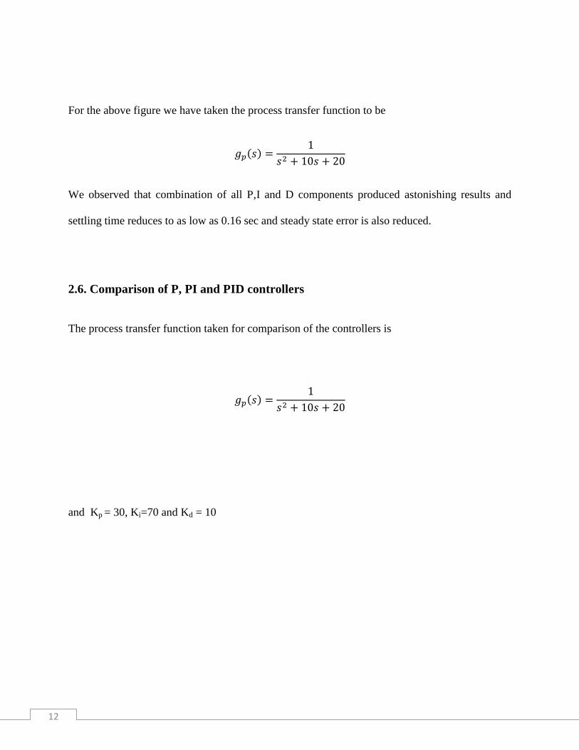
For the above figure we have taken the process transfer function to be
( )
We observed that combination of all P,I and D components produced astonishing results and
settling time reduces to as low as 0.16 sec and steady state error is also reduced.
2.6. Comparison of P, PI and PID controllers
The process transfer function taken for comparison of the controllers is
( )
and Kp = 30, Ki=70 and Kd = 10

13
Figure 6 Only-P,PI,PD,PID responses
It can be easily concluded that the proportional term is maximum responsible for change in
output , the integral term is responsible for decreasing the steady state error and the derivative
term is responsible for decreasing the rise time and overall PID controller is responsible for
better results due to decrease in settling time.

14
2.7. Examples of processes
2.7.1. Proportional Control of a first order process
Let us consider a process transfer function of a stirred tank-reactor. Where the manipulated
variable is the heater power (kW) and the output is temperature (˙C)
( )
Assuming a step input response and taking different values of Kp (1, 5, 10)
Figure 7 Proportional Control of a first order process by varying Kp (1,5,10)

15
Figure 8 Error in Proportional Control of a first order process
It can be observed that increasing the Kp reduces the offset and speeds up the response. Kp can
be increased up to a certain level beyond which the process will be unstable.
2.7.2. PI Control of a first order process
Let us consider a same process transfer function of a stirred tank-reactor. Where
( )
Assuming a set point change of 1˙C and taking different values of τi (0.25,5) with fixed
Kp=5 kW/˙C and simulating it we obtain the following figure

16
Figure 9 PI Control of a first order process by varying τi (0.25,1,5)
Figure 10 Error in PI Control of a first order process

17
We can see that for smaller integral time there is oscillatory performance for both manipulated
input and controlled output. The oscillatory performance is viewed as unfavorable to process
parameters.
2.7.3. P-only Control of a third order process
The process transfer function taken here is
( )
And plotting the graphs for input and output with Kp (1,5,10)
Figure 11 P-only Control of a third order process Kp = 1, 5,10

18
Figure 12 Error in PI Control of a first order process
2.8. Closed loop oscillation based tuning
There are three tuning parameters in a PID controller. If these are adjusted in random
fashion then it may take a while for obtaining satisfactory performance. And also each tuning
parameter will result in a different set of tuning parameter. Different kinds of algorithms have
been developed for controller tuning. The first widely used algorithm for PID tuning was
developed by Ziegler and Nichols in 1942.

19
2.8.1. Ziegler-Nichols Closed-loop method
Ziegler-Nichols Closed-loop method was the first proper algorithmic method for tuning the
PID controllers. It is not widely used today because closed-loop behavior tends to be oscillatory
and sensitive to uncertainty. We study this technique as it is the base for commonly used
automatic tuning.
2.8.2. Steps for Ziegler-Nichols Closed-loop method tuning
Taking P-only controller the magnitude of Kp is increased so as to get perfect oscillation
The value of proportional gain obtained is termed as critical (or ultimate) gain, kcu and
peak-to-peak is called ultimate period Pu .
The process transfer function used to determine the tuning parameters is
( )
( )( )( )
Figure 13 Determination of Ziegler-Nichols parameters
From the graph we obtained the values of Kcu = 10 & Pu=6.2 sec

20
2.8.3. Ziegler-Nichols Closed-loop method tuning
Ziegler-Nichols suggested tuning parameter rules that result in less oscillatory response
and are less sensitive to change in process conditions.
Table 1 Ziegler-Nichols tuning parameters
Controller Type Kc τi τd
P-only 0.5Kcu ---- ----
PI 0.45Kcu Pu/1.2 ----
PID 0.6Kcu Pu/2 Pu/8
Figure 14 Comparison of Ziegler-Nichols P,PI,PID tuning rules of controlled variable

21
Figure 15 Comparison of Ziegler-Nichols P,PI,PID tuning rules of manipulated variable

22
Chapter 3: Control Structures

23
3.1. Cascade Control
In cascade control configuration, there is one manipulated variable and more than one
measurement. It is an alternative to consider if direct feedback control using the primary variable
is not satisfactory and a secondary variable measurement is available. Cascade control uses the
output of primary controller to manipulate the set point of secondary controller.
The basic principle of cascade control is that if the secondary variable responds to the
disturbance sooner than the primary variable. So, it provides a possibility to capture and nullify
the effect of the disturbances before it propagates into the primary variable.
There are two measurements taken from the system and used in their respective control loops.
In the outer loop, the controller output is the set point of the inner loop. The outer loop is called
primary loop and the inner loop is called secondary loop. If the outer loop variable changes, it
affects in the set point of inner loop. The inner loop experiences an error signal and produces a
new output due to the change in set point. Cascade control provides better control of the outer
loop variable than is accomplished by a single variable system. The main feature of cascade
control is to divide an difficult control process into two portions; where by a secondary loop is
formed around major disturbances, leaving only minor disturbances to be controlled by the
primary controller.
3.1.1. Features of Cascade Control
More than one measurement , but one manipulated variable
Two feedback loops are nested
The output of primary controller serves as the input for secondary controller

24
Useful in case of eliminating effect of disturbances that move through the system slowly
Increases stability characteristics
Insensitive to modeling errors
Variation of primary variable decreases
The secondary controller eliminates the disturbances arising within the secondary loop
before they affect the primary variable
The proportional gain value of secondary controller is high, moreover , the offset value
associated with proportional mode can be easily removed by integral action of primary
controller.
3.1.2. Advantage of Cascade Control
Better control of primary loop
Faster recovery from disturbances
Natural frequency of the system increase
Effective magnitude of time lag decreases
Dynamic performance increases
Figure 16 Block diagram of cascaded structure

25
3.2. FeedForward Control
The conventional feedback control loop can never achieve perfect control. It is difficult on
the part of conventional loops to keep the set point at desired position continuously. This
happens because a feedback controller reacts only after it detects a deviation in the value of the
output from the desired set point. Unlike feedback systems, a feedforward control configuration
measures disturbances directly and takes action to abolish its impact on the process output.
Theoretically these controllers have potential for perfect control.
The control strategy of feedforward control , corrective action is taken in order to minimize
the deviation of controlled variable which might can disturb the control variable. The signals
which have the potential to upset the process are transmitted to the controller. The controller
makes accurate computation on these signals and calculate the new values of the manipulated
signals and send those values to the final control element, Therefore, the control variable remains
unchanged in spite of change in load.
3.2.1. Features of Feedforward Control
It is quite different from conventional feedback controllers(P, PI, and PID)
It is a special purpose computing machine
The effectiveness of the controller require through knowledge of the process model
3.2.2. Advantages of Feedforward Control
It acts before the effect of a disturbance has been felt by the system
Good for slow processes or with significant dead time
It doesn‟t introduce instability in the closed loop response.

26
3.2.3. Feedforward Control is used if
The physical and chemical properties are well known.
The variables in the equation can be easily measured.
There is no significant process disturbance.
The accuracy of measurement must be high.
Figure 17 Block diagram of feedforward contro structure
3.3. Feedforward- Feedback Control
If we can measure the up-stream disturbances, then we can take anticipatory control action
that nullifies the disturbance affecting the process. Feedforward control depends on the use of
open loop inverses; hence it is susceptible to the impact of modeling errors. Thus, we can easily
supplement feedforward control by some feedback control, so as to correct any miscalculation
involved in the anticipatory control action inherent in feedforward control. The feedfoward
control cancels the effect of the measured disturbance. Feedback acts as the system‟s watchdog
.The effect of load change other than the measured disturbance will be corrected by the feedback
system. Feedback alone must absorb the variations by feedback action only.

27
Figure 18 Block diagram of feedback-feedforward control structure
3.4. Comparison of cascade, simple feedback and feedforward-feedback structures
Let the transfer function of system be
( )( )
( )
( )
Gc2 = 4
Gm1=0.05
Gm2=0.2

28
From the block diagram we can get
Figure 19 Step response of cascaded and simple feedback structures with their
corresponding errors (Kp=4)

29
Figure 20 Step response of cascaded and simple feedback structures with their
corresponding errors (Kp=10)
From the above figures we can conclude that cascade control provides better control of the outer
loop variable than is accomplished by a single variable system and also error is also less.
Figure 21 Comparison of cascaded, simple feedback and feedback-feedforward structures
The above figure clearly states that the best control structure in terms of performance (settling
time) is feedback-feedforward(5 sec)followed by cascaded(20 sec) and simple feedback(40 sec)

30
Chapter 4: Internal Model Control

31
4.1. Internal Model Control
An internal model is a postulated neural process that simulates the response of the control
system in order to estimate the outcome of a control command. Internal models can be controlled
by either feed-forward or feedback control. Feed-forward control calculate its input into a system
using only the current state and it‟s model of the system. It does not use feedback control. So, it
cannot correct all errors in its control. In feedback control, some of the output of the system is
fed back into the system‟s input and the system became capable to make adjustments or
recompense for errors from its desired output. Two primary types of internal models have been
projected: i) forward models and ii) inverse models. In simulations, models are often combined
together to resolve more complex movement tasks.
Figure 22 General IMC structure

32
4.2. IMC Background
The main advantage of IMC is that it provides a transparent framework for control system
design and tuning. The IMC control structure can be formulated in the standard feedback control
structure. For many processes, this will result in a standard PID controller. This is satisfying
because we can use standard equipment and algorithms to implement an “advanced” control
concept. The IMC design procedure is same as that of the open loop control design procedure.
A factorization of the process has been performed for which the resulting controller would
be stable. If the controller is stable and the process is stable, then the overall controlled system is
stable. In the design of IMC there is a restriction that the process must be stable. IMC is able to
compensate for disturbances and model uncertainty, where as in case of open loop control
design it is not possible.
Let us consider the closed loop response for IMC for the following process
( ) ( )
( )( )
( )

33
Figure 23 Step change response of an IMC controller
Figure 24 Error response of an IMC controller

34
The minimum value of λ that assures closed loop stability is found to be 0.9 in which
there is perfect oscillations
Figure 25 Minimum value of λ that assures closed loop stability
35
Chapter 5: Conclusion

36
Conclusion
It can be concluded that PID controller has all the necessary dynamics: fast reaction on change of
the controller input(D mode), increase in control signal to lead error to zero(I mode) and suitable
action inside control error area to eliminate oscillations (P mode)
Among the different control structures, the feedback-feedforward control structure faster in
response
Table 2: Response of different parameters with increase in Kp, Ki, Kd
Parameter
(increase) Rise time Overshoot Settling time
Steady-state error
Decrease Increase Small change Decrease
Decrease Increase Increase Decrease
significantly
Minor decrease Minor decrease Minor decrease No change

37
Reference
[1] Bhanot Surekha: Process control principles and applications, Oxford University Press, 2008, pbk,
ISBN: 0195693348
[2] Bequette B. wayne: Process control modeling, design and simulation
[3] Strphanopoplos George: Chemical process control
[4]http://instrumrntationandcontroller.blogspot.com/2011/05/cascade_controlsystem.html
[5] http:// www.sapiensam.com/control/index.htm
[6] http:// www.myengineeringsite.com/2009