comparing two means - university of illinois at chicagohomepages.math.uic.edu/~bpower6/stat101/two...
TRANSCRIPT
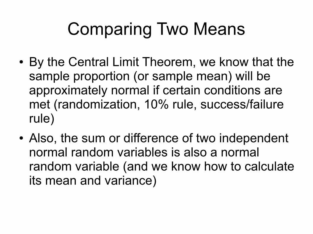
Comparing Two Means● By the Central Limit Theorem, we know that the
sample proportion (or sample mean) will be approximately normal if certain conditions are met (randomization, 10% rule, success/failure rule)
● Also, the sum or difference of two independent normal random variables is also a normal random variable (and we know how to calculate its mean and variance)

Recall how to add/subtract normal r.v.s
X is Normal with μX=60 and σ
X=4
Y is Normal with μY=45 and σ
Y=8
X and Y are independentWhat are the distributions of X+Y and X-Y?
● X+Y is normal with mean μX+Y
=60+45=105, σ
X+Y=√(42+82)=8.944
● X-Y is normal with μX-Y
=60-45=15, σX-Y
=8.944
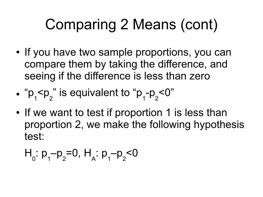
Comparing 2 Means (cont)● If you have two sample proportions, you can
compare them by taking the difference, and seeing if the difference is less than zero
● “p1<p
2” is equivalent to “p
1-p
2<0”
● If we want to test if proportion 1 is less than proportion 2, we make the following hypothesis test:H
0: p
1–p
2=0, H
A: p
1–p
2<0

Example: Arthritis in Adults over 65
Survey results: 403 out of 1019 men have arthritis, 531 out of 1068 women have arthritis.
● Assume conditions are met for CLT.● Create a 95% confidence interval for the
difference in proportions of men and women who have arthritis.
● p1 : sample proportion for women
● p1 is approx normal with mean 531/1068=.4972
and s.d. √(.4972*.5028/1068)=.0153

Example: Arthritis (cont)
● p2: sample proportion for men
● p2 is approx normal with mean 403/1019=.3955,
and s.d. √(.3955*.6045/1019)=.0153● So the sample difference p
1-p
2 is also
approximately normal with mean .4972-.3955 =.1017 and s.d √(.01532+.01532) =.0216
● A 95% confidence interval is .1017±1.96*.0216, i.e. .0594 to .1440

Example: Arthritis (cont)● 95% confidence interval for the difference of
proportions of women and men is 0.0594 to 0.1440
● This means we are 95% confidence that the proportion of women 65 and older is between 5.9% and 14.4% greater than that of men.
● Because the interval is entirely above 0, this means we are 95% confident that women are more likely to get arthritis.
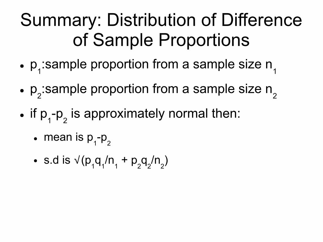
Summary: Distribution of Difference of Sample Proportions
● p1:sample proportion from a sample size n
1
● p2:sample proportion from a sample size n
2
● if p1-p
2 is approximately normal then:
● mean is p1-p
2
● s.d is √(p1q
1/n
1 + p
2q
2/n
2)

Example: Parent's Attitudes & Smoking
● Survey Results: Teens whose parents disapproved: 57 out of 284 started smoking; teens whose parents were lenient: 12 out of 41 started smoking. Create a 95% confidence interval
● Say p1 is proportion for lenient parents, p
2 for disapproving
parents● mean of p
1-p
2 is 12/41 – 57/284 = .09198
● p1=.2927, q
1=.7073. p
2=.2007, q
2=.7993
● SE=√(.2927*.7073/41 + .2007*.7993/284)=.0749● CI = .0920±1.96*.0749, that is -.055 to .239
Because the CI includes 0, we can not say with 95% confidence that a disapproving attitude of the parents makes teens less likely to smoke
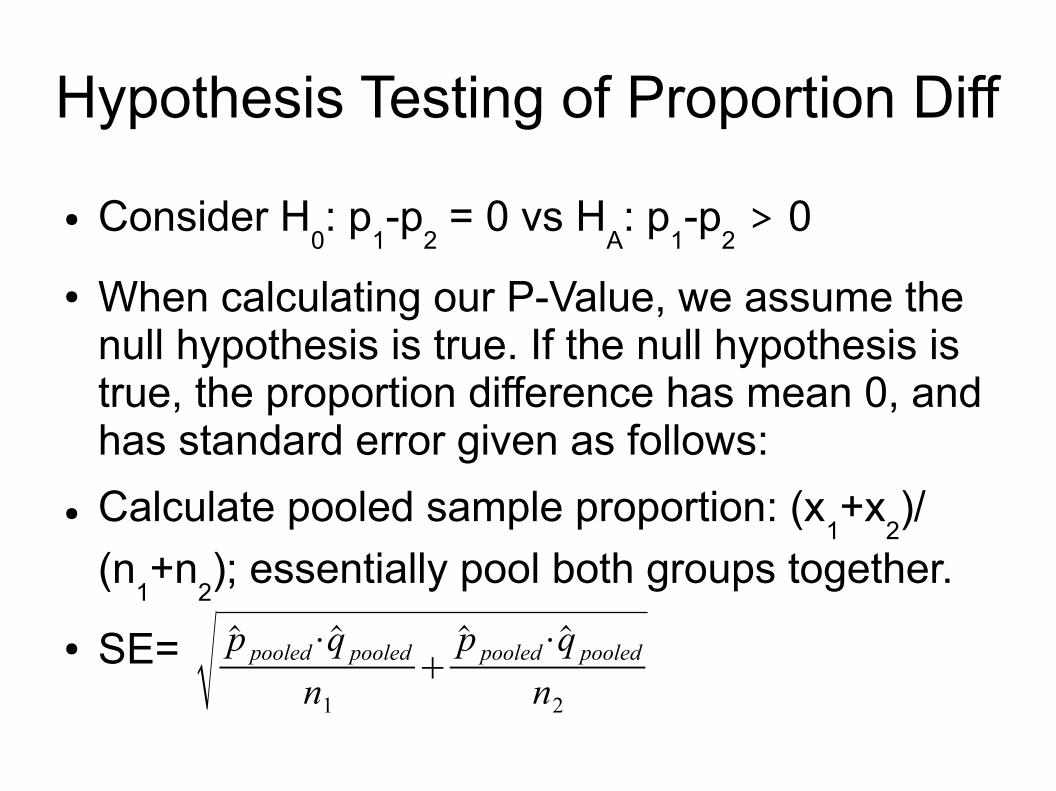
Hypothesis Testing of Proportion Diff
● Consider H0: p
1-p
2 = 0 vs H
A: p
1-p
2 > 0
● When calculating our P-Value, we assume the null hypothesis is true. If the null hypothesis is true, the proportion difference has mean 0, and has standard error given as follows:
● Calculate pooled sample proportion: (x1+x
2)/
(n1+n
2); essentially pool both groups together.
● SE= √ p̂ pooled⋅q̂ pooledn1+p̂ pooled⋅q̂ pooled
n2

Example: Reproductive Clinic● Clinic reports 43 live births to 151 women under
38, 6 out of 81 for women 38 and older. Let p1
be the proportion for women under 38, p2 for 38
and older. For a 5% significance level, is there evidence that the true proportions are different?
● H0: p
1-p
2 = 0 vs H
A: p
1-p
2 ≠ 0
● Note that this is a 2-tailed test. We need to calculate z first to find the P-value
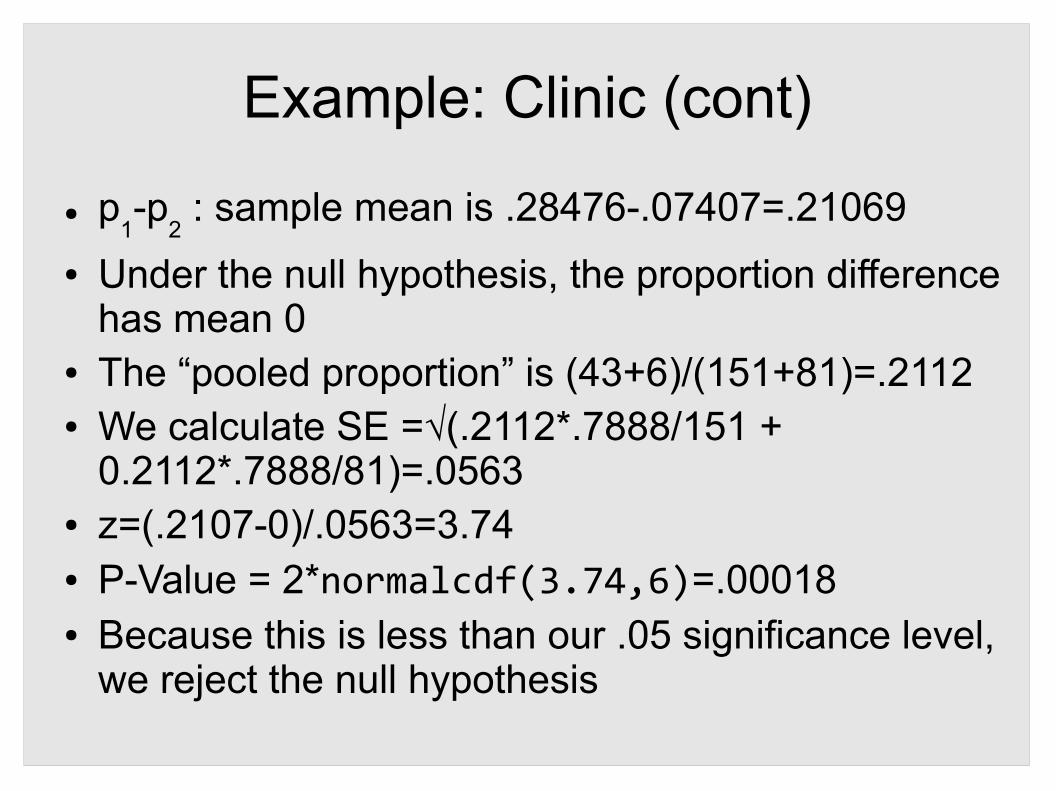
Example: Clinic (cont)
● p1-p
2 : sample mean is .28476-.07407=.21069
● Under the null hypothesis, the proportion difference has mean 0
● The “pooled proportion” is (43+6)/(151+81)=.2112● We calculate SE =√(.2112*.7888/151 +
0.2112*.7888/81)=.0563● z=(.2107-0)/.0563=3.74● P-Value = 2*normalcdf(3.74,6)=.00018● Because this is less than our .05 significance level,
we reject the null hypothesis
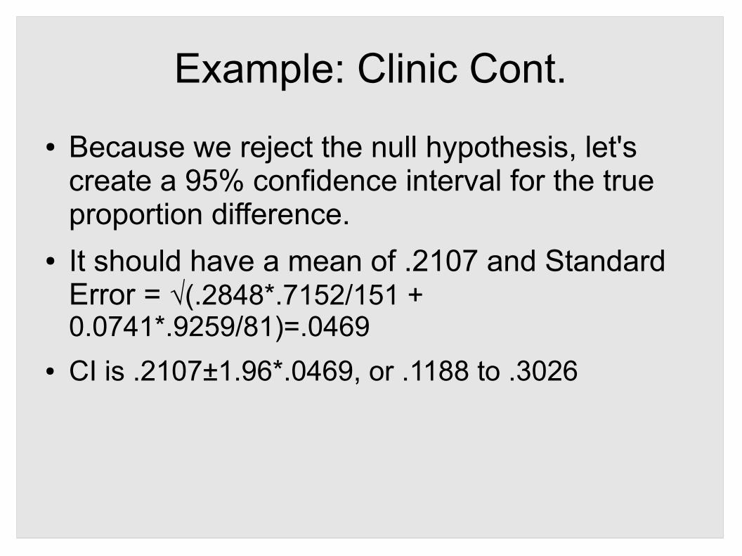
Example: Clinic Cont.● Because we reject the null hypothesis, let's
create a 95% confidence interval for the true proportion difference.
● It should have a mean of .2107 and Standard Error = √(.2848*.7152/151 + 0.0741*.9259/81)=.0469
● CI is .2107±1.96*.0469, or .1188 to .3026

Inferences about mean● If you take sample data, the sample mean will
be normally distributed if the conditions for CLT are met.
● Confidence Interval: x ± z*SE(x)● SE(x) = σ/√n if σ is known● SE(x) = s/√n if σ is unknown and n≥30
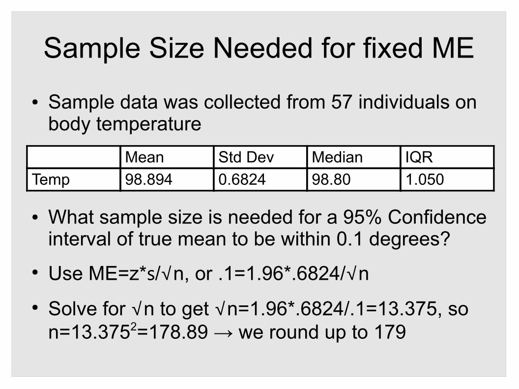
Sample Size Needed for fixed ME
Mean Std Dev Median IQRTemp 98.894 0.6824 98.80 1.050
● Sample data was collected from 57 individuals on body temperature
● What sample size is needed for a 95% Confidence interval of true mean to be within 0.1 degrees?
● Use ME=z*s/√n, or .1=1.96*.6824/√n● Solve for √n to get √n=1.96*.6824/.1=13.375, so
n=13.3752=178.89 → we round up to 179

Example: On-time flights● Each month from 1995 to 2006 (144 months) the
% of on-time flights was recorded. The mean percentage of on-time flights was 80.2986% with a standard deviation of 4.80694. Construct a 90% confidence interval for the true mean.
● z* for 90% CI is invNorm(.95)=1.6448 ● A 90% confidence interval of the true probability of
an on-time flight would be 80.2986±1.6448*4.807/√144
● This comes out to be 79.64% to 80.96%
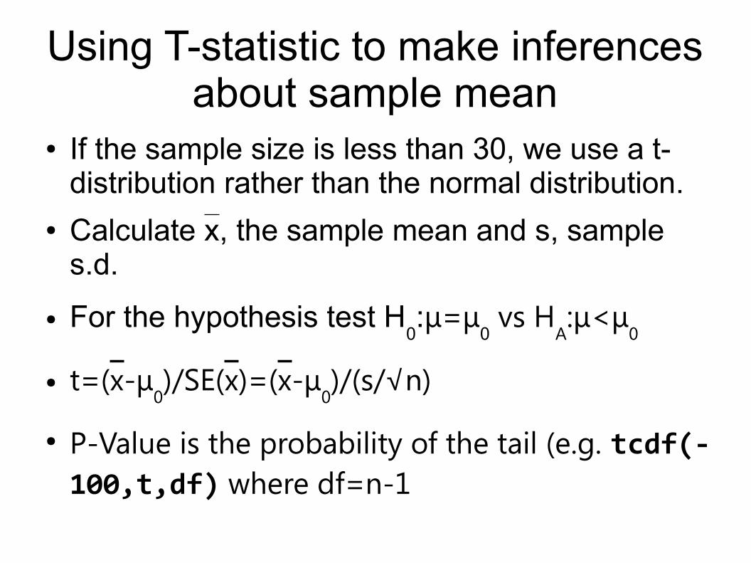
Using T-statistic to make inferences about sample mean
● If the sample size is less than 30, we use a t-distribution rather than the normal distribution.
● Calculate x, the sample mean and s, sample s.d.
● For the hypothesis test H0:μ=μ
0 vs H
A:μ<μ
0
● t=(x-μ0)/SE(x)=(x-μ
0)/(s/√n)
● P-Value is the probability of the tail (e.g. tcdf(-100,t,df) where df=n-1
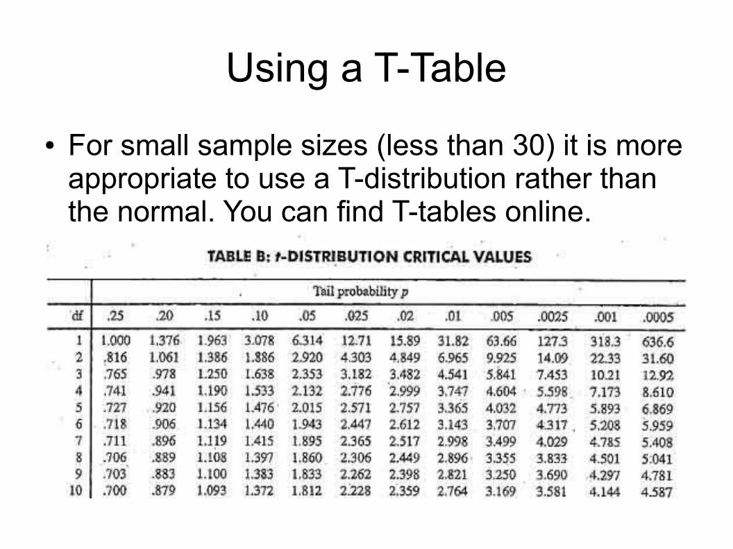
Using a T-Table● For small sample sizes (less than 30) it is more
appropriate to use a T-distribution rather than the normal. You can find T-tables online.
T -Table●
●
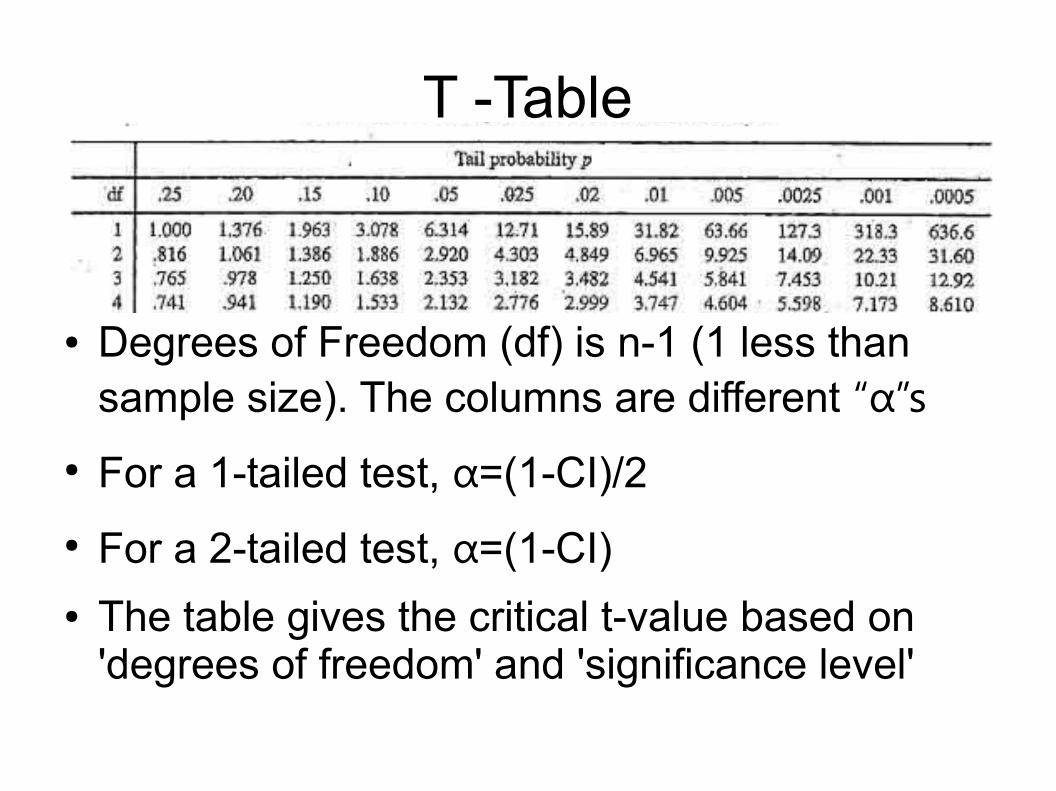
● Degrees of Freedom (df) is n-1 (1 less than sample size). The columns are different “α”s
● For a 1-tailed test, α=(1-CI)/2● For a 2-tailed test, α=(1-CI)● The table gives the critical t-value based on
'degrees of freedom' and 'significance level'

Calculating P-Value for a T distribution
● You can use “tcdf” in a TI calculator to find the exact P-value for a t-statistic
● Use “tcdf(lower, upper, df)”● ex) The P-value for t>2.32 with 4 degrees of
freedom is tcdf(2.32,100,4)=.0405● ex) the P-value for |t|>1.645 with 14 df is
2*tcdf(1.645,100,14)=1.222● A t-table is not exact enough to give a good
answer for this

Example: Microwave Popcorn● Joe thinks that the best setting for microwave
popcorn is 4 minutes on power setting 9. He says this results in less than 11% unpopped kernels. He pops 8 random bags to prove himself correct and here are the results (% unpopped): 10.1, 9.4, 9.2, 5.9, 11.9, 5.6, 13.7, 7.6
● H0: p=11%, HA: p<11%● Assuming α=.05, does this evidence support
Joe's claim?

Example: Microwave Popcorn (cont)● We can easily calculate x=9.175 and s=2.7978● SE(x)=2.7978/√8=.9892● t=(9.175-11)/.9892 = -1.845● Sample size of 8 means 7 degrees of freedom. ● P-value is tcdf(-100,-1.845,7)=.0538● This is higher than our significance level. There
is not enough evidence to reject the null hypothesis. Keep trying, Joe!