comparing incomparable survey responses: evaluating and ... · comparing incomparable survey...

Comparing Incomparable Survey Responses:Evaluating and Selecting Anchoring Vignettes

Gary King

Institute for Quantitative Social Science, 1737 Cambridge Street,

Harvard University, Cambridge MA 02138

e-mail: [email protected] (corresponding author)

Jonathan Wand

Department of Political Science, Encina Hall, Room 308 West,

Stanford University, Stanford, CA 94305-6044

e-mail: [email protected]

When respondents use the ordinal response categories of standard survey questions in

different ways, the validity of analyses based on the resulting data can be biased. Anchoring

vignettes is a survey design technique, introduced by King et al. (2004, Enhancing the

validity and cross-cultural comparability of measurement in survey research. American

Political Science Review 94 [February]: 191–205), intended to correct for some of these

problems. We develop new methods both for evaluating and choosing anchoring vignettes

and for analyzing the resulting data. With surveys on a diverse range of topics in a range

of countries, we illustrate how our proposed methods can improve the ability of anchoring

vignettes to extract information from survey data, as well as saving in survey administration

costs.

1 Introduction

Researchers have tried to ameliorate the problems of interpersonal and cross-culturalincomparability in survey research with careful question wording, translation (and backtranslation), focus groups, cognitive debriefing, and other techniques, most of which aredesigned to improve the survey question. In contrast, anchoring vignettes is a technique(developed by King et al. 2004) designed to ameliorate problems that occur when differentgroups of respondents understand and use ordinal response categories—such as (1)strongly disagree, (2) disagree, (3) neutral, (4) agree, or (5) strongly agree—in differentways. When one group of respondents happen to have comparatively higher standards forwhat constitutes the definition of ‘‘strongly agree,’’ for example, they will report system-atically lower levels of agreement than another group. Yet, some people obviously differ in

Authors’ note: Our thanks go to Amos Golan, George Judge, Doug Miller, Chris Murray, Olivia Lau, andJosh Salomon for many helpful suggestions; Emmanuela Gakidou and Ajay Tandon for data; Dan Hopkins forinsightful research assistance; and National Institute on Aging/National Institutes of Health (for grant P01AG17625-01 to King) and the Robert Wood Johnson Scholars in Health Policy Research program at the Uni-versity of Michigan (to Wand) for generous research support.

� The Author 2006. Published by Oxford University Press on behalf of the Society for Political Methodology.All rights reserved. For Permissions, please email: [email protected]

1

doi:10.1093/pan/mpl011

Political Analysis Advance Access published December 11, 2006

optimism, agreeability, mood, propensity to use extreme categories, and other character-istics, and so doing something about this ‘‘response-category differential item function-ing’’ (or DIF) should be a high priority for researchers.

The methodology of anchoring vignettes attack DIF with new types of supplementalsurvey questions that make it possible to construct a common scale of measurement acrossrespondents, along with specially designed statistical methods for analyzing the resultingdata. Anchoring vignettes have now been used to measure numerous concepts and havebeen implemented in surveys in over 80 countries by a growing list of survey organizationsand researchers in a variety of academic fields.1 In this paper, we describe this approachand develop improved statistical methods for analyzing, evaluating, and selecting anchor-ing vignettes that require fewer assumptions, can extract more information from the samesurvey questions, and should save in research costs.

Previous applications of anchoring vignettes have used as many as 12 vignettes per self-assessment question. However, adding this many additional questions for each self-assessment, or even the five used by King et al. (2004), may be prohibitively expensivein some surveys and, we show, are often unnecessary to correct DIF. In some cases, thenecessary correction may be achieved with a single vignette. In other cases, more vignettesmay be informative. In all cases, the methods we introduce to evaluate the efficacy of eachvignette to improve interpersonal incomparability should be of direct practical use toresearchers.

We begin in Section 2 by summarizing the anchoring vignettes approach. Section 3 thenprovides a more general definition of this approach, a new formalization, a more generallyapplicable analytical method, and an illustration of the methods offered. Section 4 thendevelops new ways of evaluating the information available in a set of anchoring vignettesand detecting vignettes that may be empirically unnecessary or less useful and those thatmay violate key assumptions of the technique. Section 5 gives several examples of eval-uating vignettes in practice, and Section 6 concludes. The new information our methodsreveal greatly increases the efficacy of the nonparametric estimator, making it a powerfulalternative to the parametric approach and one that requires considerably less stringentassumptions.

2 The Technique of Anchoring Vignettes

A variant of a question asked in numerous surveys seeks to measure what political scien-tists call political efficacy:

How much say do you have in getting the government to address issues that interest you? (1) No

say, (2) Little say, (3) Some say, (4) A lot of say, (5) Unlimited say.

For this question, as most others, political scientists typically theorize that each respondenthas an actual level of efficacy that may differ from the reported level due to measurement,respondent ‘‘considerations,’’ the survey interview setting, positivity bias, or other aspectsof DIF. Political scientists typically view the actual level of efficacy as a relatively objec-tive psychological state: Respondents who genuinely feel politically efficacious are morelikely to participate in politics, write letters to public officials, contribute to politicalcampaigns, debate policy with their friends, and feel more generally part of the politicalsystem. The difference between true underlying perceived political efficacy and the re-ported level may differ due to a variety of measurement factors including idiosyncratic

1A library of anchoring vignette examples used in these and other surveys, and other materials, can be found athttp://gking.harvard.edu/vign/. Our software for analyzing anchoring vignettes is at http://wand.stanford.edu; seeWand, King, and Lau (forthcoming).

2 Gary King and Jonathan Wand

considerations of the respondent or variations in the survey interview setting. There maybe more systematic biases within groups, such as positivity bias or different standards forthe categories on the scale. We address the issue of these systematic differences in the useof scale within groups, referred to generically as DIF.

King et al. (2004) measured political efficacy with this question in surveys from Chinaand Mexico. Remarkably, the raw responses indicate that the citizens of (democratic)Mexico judge themselves to have substantially lower levels of political efficacy thancitizens of (nondemocratic, communist) China judge themselves. For example, more than50% of Mexicans but fewer than 30% of Chinese reported in these surveys having no sayin the government. The massively divergent levels of actual freedom and democracy in thetwo countries strongly suggest exactly the opposite conclusion and thus a potential prob-lem with the survey question or how it is understood. King et al. (2004) argue that both thelevels of efficacy and the standards for any particular level (i.e., DIF) vary between thecountries, and as such, the reported self-responses are incomparable between countries.

In the present example, King et al. (2004) explain the apparent paradox with theChinese in fact having lower actual levels of political efficacy than the Mexicans. How-ever, the Chinese report higher levels of say in government because they have lowerstandards for what counts as satisfying the level described by any given response category.

Reported survey responses alone cannot be used to address the issue of comparability ofscales across groups. Addressing DIF requires some measure or benchmark for the actualunobserved level of the variable that the survey question is intended to measure. To pro-vide a common reference point for people applying different standards for the same scale,one approach is to ask each respondent an additional anchoring vignette question after theself-assessment such as

[Moses] lacks clean drinking water. He would like to change this, but he can’t vote, and feels that

no one in the government cares about this issue. So he suffers in silence, hoping something will be

done in the future.

How much say does [Moses] have in getting the government to address issues that interest

him?

with the same response categories as the self-assessment. (To increase the likelihood thatrespondents think of the vignette as describing someone like themselves except for thecontent of the vignette, the hypothetical individuals are given names appropriate to thelanguage and culture and when possible also indicating the same sex as the respondent.)

Because the reported answer to the self-assessment question includes both the actuallevel of efficacy and DIF, we cannot separate the two without further information. Theanchoring vignette question provides that additional information, since Moses has thesame actual level of efficacy no matter which respondent in which country is queried.Thus, any systematic variation in answers about the Moses question can only be due toDIF. By assuming only that the DIF that a respondent applies to his or her self-assessmentis the same as the DIF that this person applies to the vignette question, we can ‘‘subtractoff’’ the DIF from the self-assessment to yield a DIF-free estimate of the actual level ofpolitical efficacy. In the simplest (nonparametric) method of analysis, we can correct forDIF by recoding the self-assessment response relative to the vignette response as (1) lessthan, (2) equal to, or (3) greater than the vignette response. In fact, although the rawresponses had the Chinese judging themselves to have considerably more efficacy thantheMexicans judged themselves to have, the DIF-corrected responses indicates the reverse:whereas only about 12% of Mexicans judged themselves to have less political efficacy than‘‘Moses’’ in the vignette above, 40% of the Chinese judged themselves to have less efficacythan Moses who suffers in silence (see King et al. 2004, 196).

Comparing Incomparable Survey Responses 3

To be more explicit, two assumptions enable us to regard this trichotomous recodedanswer as DIF free and freely compared across different groups of people. The first isresponse consistency, which is the assumption that each respondent uses the survey responsecategories in the sameway to answer the anchoring vignette and self-assessment questions.Different people may have different types of DIF, but any one person must apply the sameDIF in approximately the same way across the two types of questions. Second is vignetteequivalence, which is the assumption that the level of thevariable represented in thevignetteis understood by all respondents in the sameway apart from randommeasurement error. Ofcourse, even when respondents understand vignettes in the same way on average, differentrespondents may apply their own unique DIFs in choosing response categories.

Thus, unlike almost all existing survey research, anchoring vignettes allow and ulti-mately correct for the DIF that may exist when survey respondents choose among theresponse categories, but they assume like most previous research the absence of DIF in the‘‘stem question.’’ It seems reasonable to focus on response-category DIF as the mainsource of the problem because the vignettes describe behaviors or psychological statesintended to be more objective and for which traditional survey design advice to avoid DIF(such as pretesting, cognitive debriefing, and writing questions concretely) is likely towork better (although the methods described here may also help to identify problematicvignettes). In contrast, response categories describe much more subjective feelings andattitudes attached to words or phrases that are by their nature imprecise; the responsesshould therefore be harder to lay out in concrete ways and avoid DIF without anchoringvignettes. This point also seems consistent with the finding in the literature that traditionalsurvey design advice can work especially badly for Likert-type response scales (Schwarz1999).

One issue with the DIF correction in the example thus far is that the five-categorypolitical efficacy response is reduced to only a three-category DIF-corrected variable, andso information may have been lost. As it turns out, however, we can recover additionalinformation by adding more vignettes. For example, King et al. (2004) also use thisvignette:

[Imelda] lacks clean drinking water. She and her neighbors are drawing attention to the issue by

collecting signatures on a petition. They plan to present the petition to each of the political parties

before the upcoming election.

with the same survey question and response categories. If survey respondents rank the twovignettes in the same order, we can create a DIF-free variable by recoding the self-assessment into five categories: (1) less than Moses, (2) equal to Moses, (3) betweenMoses and Imelda, (4) equal to Imelda, and (5) greater than Imelda. Of course, we canobtain considerably more discriminatory power by adding more vignettes. In the politicalefficacy example, King et al. (2004) use five vignettes presented to the respondent inrandom order.

More vignettes of course also come with an additional assumption: that all the respond-ents understand the vignettes as falling along the same unidimensional scale, even if theydo not use the scale and response categories in the same way. In the vignettes above, forexample, Imelda presumably has more political efficacy than Moses, but if many respond-ents indicated otherwise, this might be an indication of multiple dimensions being tappedby the vignettes. Even if unidimensionality holds as assumed, using multiple vignettesgives rise to other potential challenges. For example, random error in perceptions orresponses may produce inconsistencies in vignette rankings. Other respondents may notperceive the difference between some vignettes and may give them tied responses. We dealwith these issues in this study.


Finally, we note that asking vignettes may seem like an expensive technique since itrequires adding multiple questions to a survey to correct for each self-assessment question.In fact, however, King et al. (2004) develop a statistical technique that enables one to askanchoring vignettes of only a small random subsample and to still statistically correct forDIF using parametric assumptions; the same technique can also be applied to respondentswho were not asked all questions. Alternatively, one can include the vignettes on thepretest and not the full survey or include only a subset on the main survey. Or one canadd, for each self-assessment, only one additional item, where each quarter of the respond-ents are asked a different vignette (although this presumes that the assumptions underlyingthe use of the vignettes to anchor the self-responses have already been verified with otherdata). It is also possible to choose vignettes adaptively, so that we give each respondentdifferent vignettes depending on his or her response to previous questions. A parametricmethod is available that enables one to save survey administration costs in these and otherways. The mostly nonparametric methods we introduce here minimize statistical modelingassumptions and so provide a useful complement to parametric modeling.

3 Estimation Strategy

Our estimation strategy first extracts all known information via a fully nonparametricapproach, without making any additional assumptions. We then supplement this nonpara-metric information with a parametric approach that, by making some additional assump-tions, extracts additional information. The parametric supplement also makes it easy toanalyze the nonparametric data to compute predictions, causal inferences, and counter-factual questions.

3.1 The Nonparametric Estimator

We now offer a simple generalization of the nonparametric approach, described as simplerecodes in Section 2 and King et al. (2004). Let y be the self-assessment response andz1; . . . ; zJ be the J vignette responses, for a single respondent. The same discrete ordinalresponse choices (e.g., unlimited say, a lot of say, some say, etc.) are offered to the re-spondent for each of the questions. For respondents with consistently ordered rankings onall vignettes (zj�1 , zj; for j5 2; . . . ; J), we create the DIF-corrected self-assessment bythe recodes described in Section 2, which in mathematical notation is

C 5

1 if y, z12 if y5 z13 if z1 , y, z2

..

. ...

2J þ 1 if y. zJ :

8>>>>><>>>>>:

ð1Þ

Since this section considers one survey respondent at a time, we omit the subscriptdenoting the respondent.2

The only remaining issue is how to generalize equation (1) to allow for respondentswho give tied or inconsistently ordered vignette responses. We do this by first checking

2The ordering of vignettes is normally chosen by the researchers, but it is also possible to draw upon a consensusordering by the respondents, so long as only one ordering is used for all respondents for the analysis. Differencesbetween hypothesized ordering of the researchers and the consensus ordering may fruitfully be used for di-agnosing problems in the survey instruments, particularly when translating the questions for use in differentlanguages.


which of the conditions on the right side of equation (1) are true and then summarize Cwith the vector of responses that range from the minimum to maximum values among allthe conditions that hold true. Values of C that are intervals (or vector valued), rather thanscalar, represent the set of inequalities over which the analyst cannot distinguish withoutfurther assumption; we refer informally to cases that have interval values as being cen-sored observations.

Table 1 gives all 13 examples that can result from two vignette responses and a self-assessment. Examples 1–5 have both vignettes correctly ordered and not tied, with theresult for C being a scalar. The vignette responses are tied in examples 6–8, whichproduces a censored value for C only if the self-assessment is equal to them. Examples9–13 are for survey responses that incorrectly order the vignettes. Within each set, theexamples are ordered by moving y from left to right.

This generalized definition for C clarifies the impact of ties (as in examples 6 and 8) andinconsistencies (as in examples 9 and 13) among the vignettes that occur in a group strictlygreater than or less than y. Note that all four of these examples in the table have scalar(uncensored) values for C. This is appropriate since we might reasonably expect respond-ents to be more likely to give some tied or inconsistent answers among vignettes that arefar from their own self-assessment even when they correctly rank the vignettes that matternear their own value. For example, if we are measuring height and a respondent knew hisor her height to within an inch, he or she still might have difficulty correctly ranking theheights of two trees 200 and 206 feet tall, swaying in the breeze. Yet, the same respondentwould presumably have no difficulty understanding that both trees are taller than himselfor herself. We thus regard the respondent’s misordering of vignettes in this way to not haveany censoring effect on the estimate.

3.2 A Parametric Supplement

The nonparametric estimator discussed in Section 3.1 recodes the vignettes and self-assessment questions into a single DIF-free variable C. Since this unusual dependent

Table 1 All examples with two vignettes: this table gives calculations for the nonparametricestimator C for all possible examples (sans nonresponse) with two vignette responses, z1 and z2

(intended to be ordered as z1 , z2), and a self-assessment, y

Surveyresponses

1 2 3 4 5

Example y , z1 y 5 z1 z1 , y , z2 y 5 z2 y . z2 C

1 y , z1 , z2 1 0 0 0 0 f1g2 y 5 z1 , z2 0 1 0 0 0 f2g3 z1 , y , z2 0 0 1 0 0 f3g4 z1 , y 5 z2 0 0 0 1 0 f4g5 z1 , z2 , y 0 0 0 0 1 f5g6 y , z1 5 z2 1 0 0 0 0 f1g7 y 5 z1 5 z2 0 1 0 1 0 f2, 3, 4g8 z1 5 z2 , y 0 0 0 0 1 f5g9 y , z2 , z1 1 0 0 0 0 f1g10 y 5 z2 , z1 1 0 0 1 0 f1, 2, 3, 4g11 z2 , y , z1 1 0 0 0 1 f1, 2, 3, 4, 5g12 z2 , y 5 z1 0 1 0 0 1 f2, 3, 4, 5g13 z2 , z1 , y 0 0 0 0 1 f5g


variable has a scalar value for some observations and multiple values for others, we nowdevelop a way to analyze such variables. In fact, the method described here would alsoapply to survey questions that permitted respondents to choose among any range of re-sponse categories, rather than a single one. Such questions do not appear to be usedfrequently, but they may be useful in tapping into respondents’ central tendencies as wellas uncertainties in a single question.

Consider the simple example of drawing a histogram of the results of C. If C wereentirely scalar valued, we would do what we always do: Sort the values of C into eachcategory j ( j5 1; . . . ; 2J þ 1), compute the proportion pj in each, and plot one bar for eachcategory with size proportional to pj.

The key issue is what to do when C is a range (or vector valued) instead of a scalar. Onesimple possibility would be to discard the vector-valued observations. This would obvi-ously waste information, at best, and of course, it may introduce selection bias as well.Another simple approach would be to take the vector values and spread the area evenlyacross all the members of the vector-valued set. This is what King et al. (2004) did, but theallocation rule they employed is obviously an assumption that should be consideredcarefully rather than used automatically. If the assumption is wrong, it will bias resultstoward a uniform density (a flat histogram) and so may cause one to obliterate features ofthe true frequency distribution.

In this section, we move beyond these simplistic approaches and seek to allocate thevector-valued responses to categories as best as possible so that we simultaneously useinformation about both the scalar and vector values of the variable C. Our approach fordisplaying C in a single-dimensional representation, such as a histogram, is to distributeeach vector-valued response according to the proportion of ‘‘similar’’ respondents whochose the categories spanned by the vector. We thus estimate the proportion in each of thespanned categories using a generalization of the ordered probit model that allows ‘‘cen-sored’’ values corresponding to our vector values. In this way, we obtain an estimate of theproportion of the sample in each category of C, which can be used to construct a histogramor for other analyses.

To define our approach, we begin with the classic ordered probit and then generalize intwo ways. First denote Yi (for respondent i5 1; . . . ; n) as a continuous unobserved de-pendent variable and xi as a vector of explanatory variables (and for identification, with noconstant term). If this is used as a predictive rather than causal model, as would beappropriate if the goal were to draw a histogram or for other descriptive purposes, what-ever variables that might be associated with the outcome should be included. Covariateselection for causal purposes would follow the same rules as for a traditional orderedprobit model. Then, we model Yi as conditionally normal with mean xib and variance 1. IfYi were observed, the maximum likelihood estimate of b would simply be the coefficientfrom a linear regression of Yi on xi.

However, instead of observing Yi, we instead see Ci through a specific observationmechanism. Thus, for scalar values, the mechanism is

Ci 5 c if sc�1 � Yi , sc ð2Þ

with thresholds sc (where s05�N, s2Jþ15N, and sc�1, sc and for c5 1; . . . ; 2J þ 1).Under this model, the probability of observing an outcome in category c is simply

PrðC 5 c j x0Þ5Z sc

sc�1

Nðy j x0b; 1Þdy ð3Þ


for a given vector of values of the explanatory variables, x0. This of course is exactly theordered probit model.

We now generalize this model in the first of two ways by adding notation for vectorvalues of C, which we do by altering the observation mechanism in equation (2) to

Ci 5 c if sminðcÞ�1 � Yi , smaxðcÞ: ð4Þ

This censored ordered probit model can also be used as a means of estimating causaleffects under the maintained assumptions. One would merely estimate the model andinterpret b exactly as under ordered probit (such as by using the procedures in King,Tomz, and Wittenberg 2000). Researchers could estimate the probability of a respondentanswering in any individual category by using equation (3).3

To compute histograms, and for occasional other purposes, we are able to add consider-able robustness by introducing a second generalization of the classic ordered probit modelthat conditions the calculation of the probability of being in a specific (single) category con the observed vector or scalar ci (using a technique analogous to that in King [1997] andKing et al. [2004], Appendix B). This conditional calculation is simply

PrðC 5 c j x0; ciÞ5PrðC 5 cjx0ÞPa2ci

PrðC 5 ajx0Þ; for c 2 ci;

0; otherwise;

8<: ð5Þ

where the usual unconditional probability Pr(C 5 cjx0) is defined in equation (3). The newexpression in equation (5) conditions on ci by normalizing the probability to sum to onewithin the set ci and zero outside that set. For scalar values of ci, this expression simplyreturns the observed category: Pr(C 5 cjxi, ci) 5 1 for category c and 0 otherwise. Forvector-valued ci, equation (5) puts a probability density over the categories within ci,which in total sum to one.

Avirtue of this method is that predictions of scalar-valued observations are fixed at theirobserved values, independent of the model, and thus are always correct no matter howmisspecified the model. In addition, predictions of vector-valued observations are re-stricted to within their observed range, also with certainty and independent of modelingchoices. The method uses all available information in the self-assessment, vignettes, andexplanatory variables to estimate the distribution of frequencies for the vector-valuedobservations rather than merely assuming an arbitrary distribution ex ante. The robustnessof this conditional approach is directly related to size of the range. Analogous to theinfluence of the proportion of missing data in multiple imputation, a smaller range ofvector values offers relatively greater confidence in the resulting histogram independent ofthe modeling assumptions, since the result is bounded by the known information in thedata (Heitjan and Rubin 1990; King et al. 2001).

3.3 Empirical Illustration

King et al. (2004) analyze political efficacy data in China and Mexico and show that, withan anchoring vignettes DIF correction, the ranking of the two countries switches compared

3If two response categories are observed as part of the vector-valued C for the same set of observations and for noothers, some of the threshold parameters are not identified. The nonidentification in this unusual special case ispartial in the sense that the likelihood still indicates the mass in the sum of the two categories. The problem canbe easily addressed by combining the two categories or by using information to construct a prior for the s’s.


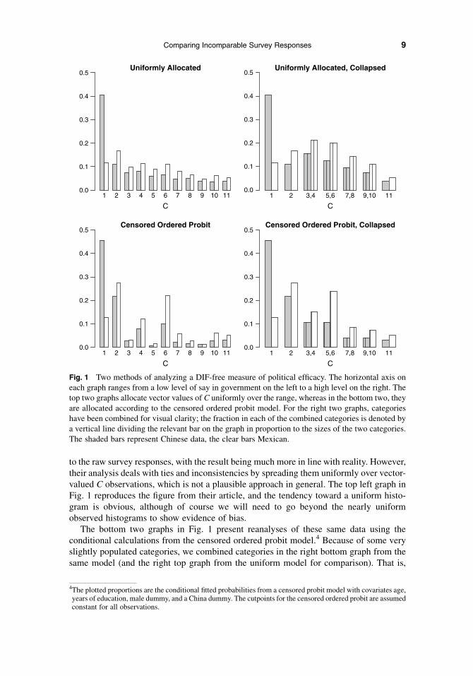
to the raw survey responses, with the result being much more in line with reality. However,their analysis deals with ties and inconsistencies by spreading them uniformly over vector-valued C observations, which is not a plausible approach in general. The top left graph inFig. 1 reproduces the figure from their article, and the tendency toward a uniform histo-gram is obvious, although of course we will need to go beyond the nearly uniformobserved histograms to show evidence of bias.

The bottom two graphs in Fig. 1 present reanalyses of these same data using theconditional calculations from the censored ordered probit model.4 Because of some veryslightly populated categories, we combined categories in the right bottom graph from thesame model (and the right top graph from the uniform model for comparison). That is,

1 2 3 4 5 6 7 8 9 10 11

Uniformly Allocated

C

0.0

0.1

0.2

0.3

0.4

0.5

1 2 3,4 5,6 7,8 9,10 11

Uniformly Allocated, Collapsed

C

1 2 3 4 5 6 7 8 9 10 11

C

1 2 3,4 5,6 7,8 9,10 11

C

0.0

0.1

0.2

0.3

0.4

0.5

Censored Ordered Probit

0.0

0.1

0.2

0.3

0.4

0.5Censored Ordered Probit, Collapsed

0.0

0.1

0.2

0.3

0.4

0.5

Fig. 1 Two methods of analyzing a DIF-free measure of political efficacy. The horizontal axis oneach graph ranges from a low level of say in government on the left to a high level on the right. Thetop two graphs allocate vector values of C uniformly over the range, whereas in the bottom two, theyare allocated according to the censored ordered probit model. For the right two graphs, categorieshave been combined for visual clarity; the fraction in each of the combined categories is denoted bya vertical line dividing the relevant bar on the graph in proportion to the sizes of the two categories.The shaded bars represent Chinese data, the clear bars Mexican.

4The plotted proportions are the conditional fitted probabilities from a censored probit model with covariates age,years of education, male dummy, and a China dummy. The cutpoints for the censored ordered probit are assumedconstant for all observations.


because the survey question has only five response categories, and since most responsesare clustered at the low end of efficacy, some odd-numbered values of C have very smallnumbers of respondents. The result is not a methodological problem but merely an estheticone, since comparing histograms with sawtooth patterns can be visually complicated.Combining selected adjacent categories solves this problem. So that no information islost by this procedure, we add a vertical line that splits any bar representing two categorieswith area proportional to the size of the two categories.

If the uniform assumption of the top graphs were correct, the censored ordered probitmethods would pick up that information and the top and bottom rows of histograms wouldlook fairly similar. In fact, the results clearly indicate that the censored ordered probitmethods are picking up information not in the uniform allocation approach. Whereas themain difference between Mexico and China in the uniform graphs is the spike in categoryC 5 1 for China, the ordered probit methods reveal considerably more texture. In fact, thepreferred conditional approach in the bottom right graph illustrates very different patternsfor the two countries. China shows a relatively smooth exponential decline, whereas theMexico histogram indicates that the bulk of respondents have markedly higher levels ofpolitical efficacy. The result is much more consistent with what we know about the twocountries’ divergent levels of efficacy than the more modest differences revealed by theuniform assumption graph.

4 Evaluating Vignettes

Asking a random sample of Americans how often they run two marathons in a weekobviously would not yield much information about how much the respondents exercise.Similarly, different vignettes for a given self-assessment question vary in the informationthey yield about respondents. In this section, we develop a useful and relatively naturalmeasure of the information revealed by the set of vignettes used. This measure can be usedto assist in choosing a subset of vignettes for more detailed analyses or subsequent surveys.

We begin by conceptualizing each respondent’s actual level as falling on an unobservedunidimensional continuous scale broken up into the 2J þ 1 categories defining C. The setof vignettes used to create C gives meaning to each of its categories. Our task is to choosea set of vignettes to assign the most useful set of meanings to the categories of C, which weshall do by developing a measure of the discriminatory power of or information in the setof vignettes. We explain this first for the simpler case of scalar values of C and sub-sequently for scalar and vector values of C.

4.1 Information in Scalar Values of C

For simplicity, we assume in this section that C contains a single value for each observation(which occurs in the absence of ties or inconsistencies among the vignettes).We denote by pj

the proportion of observations in category j of C (for j5 1; . . . ; 2J þ 1). The resulting set ofproportions in the categories, fp1; . . . ; p2Jþ1g, define a frequency distribution of responses,such as might be portrayed via a histogram (with pj proportional to the height of bar j).

As in the case of a survey question about running twomarathons in a week, when a set ofvignettes defines C such that all respondents fall into only one of its categories, C conveysthe least possible information about the underlying continuous scale. It is true that we geta lot of information about the fitness of an individual who responds that he or she does runtwo marathons weekly, but we will not likely see many individuals of this type and so theexpected amount of information is near zero. In contrast, C is best able to discriminate


among respondents on the underlying continuous scale when vignettes are chosen to definecategories of C such that respondents are sorted equally across all the categories:

p1 5 p2 5 � � � 5 p2Jþ1 51

2J þ 1: ð6Þ

Our immediate goal, then, is to define a measure of the informativeness or discrimi-natory power of a set of vignettes for a given self-assessment question. In other words, weneed to define a continuous function H(�) that takes the set of frequencies, p1; . . . ; p2Jþ1; asarguments and returns a real number indicating the information in the frequencies andhence the information in the vignettes that define C. This real number should be ata minimum, which we will denote as zero, when one category contains all respondentsand at a maximum when respondents are spread across the categories equally. To avoidhard-to-justify application-specific assumptions about the relative importance of each ofthe categories of C, we require the arguments of H to be symmetric in that if we reorderedthe p’s, H would return the same number. The symmetry requirement could easily bedropped if such information were available for a particular application. Of course, manyfunctions satisfy these simple criteria, but we can narrow down the search to a uniquechoice by adding two more requirements, both needed to cope with the possibility ofconsidering and comparing this measure with different numbers of vignettes.

First, since more categories of C (which result from using more vignettes) should neveryield less discriminatory power, we require in the case of no ties or inconsistencies thatH be a monotonically increasing function of the number of vignettes J and hence the num-ber of categories, 2J þ 1. Second, when adding a new vignette and decomposing a categoryof C into smaller bins, the amount of expected information in the union of these smallerbins should remain the same as the original undecomposed bin and the expected infor-mation in the other unaffected bins should remain unchanged by the addition of the newvignette.

For example, suppose we begin with a single vignette (J 5 1), so that C has 2J þ 15 3categories, with proportions labeled p1, p2, and q, respectively, and we wish to computeH(p1, p2, q). The three proportions refer, respectively, to outcomes where the self-assessmenty is less than, equal to, and greater than z1. Now consider adding an additional vignettewith a value higher than the existing one: z1 , z2. This effectively breaks up the group ofrespondents with self-assessments that fall to the right of z1 (previously the third event,with frequency q) into the self-assessment falling between z1 and z2, equal to z2, andgreater than z2, and of course, the decomposition is logically consistent: q 5 p3 þ p4 þp5. Since the first two events, being less than z1 and equal to z1, have not changed with theintroduction of z2, the first two proportions, p1 and p2, are unchanged, and so we requireour measure of the information that they convey to also be unchanged.

The second criterion, then, is that we ought to be able to compute identical values of theinformation in the vignettes by applying the function to the set of all five probabilities H(p1,p2, p3, p4, p5) or by computing a weighted average of the information in grouped categoriesH(p1, p2, q) and the information in the components of the third category, H(p3, p4, p5). Moreformally, this amounts to adding a consistency requirement so that in this example

Hðp1; p2; p3; p4; p5Þ5Hðp1; p2; qÞ þ qHðp3; p4; p5Þ; ð7Þ

where the second term quantifies separately how much information the second vignetteadds. Thus, we shall require a generalization of this, which states that when multiple waysof hierarchically decomposing H(�) exist, they shall all yield identical values.


Although numerous potential candidates for H(�) exist—such as any of the measures ofincome inequality, like the Gini index, the variance, and mean absolute deviations—theessential requirements given above rule out all but one. As proved by Shannon (1949) inthe context of mathematical communications theory, the unique definition of this functionis proportional to

Hðp1; . . . ; p2Jþ1Þ5 �X2Jþ1

j5 1

pjlnðpjÞ; ð8Þ

where for convenience we define �0 ln(0) [ 0 (since lima/0þa lnð1=aÞ5 0). The func-tion H is known as entropy and has found many applied uses (Golan, Judge, and Miller1996).5

The measure of entropy is such that H 5 0 if and only if all respondents fall in only onecategory of C, the situation of minimal information. For any given J, H is at a maximumand equal to lnð2J þ 1Þ; when pj 5 1=ð2J þ 1Þ (for all j), which is a uniform frequencydistribution. The maximum entropy (and informativeness) is thus higher as the number ofvignettes J gets larger. Finally, any equalizing of the frequencies of two or more categoriesproduces an increase in H, which implies that the measure is also logically consistentbetween the extremes.

The key insight, however, is that no other measure—not the variance of the pj’s, notmean absolute deviations, not the Gini coefficient, not anything but entropy—satisfies theessential criteria set out above.

4.2 Information in Scalar and Vector Values of C

When two or more vignettes are tied or inconsistently ranked by a survey respondent, Ccan be vector valued and so the standard definition of entropy in equation (8) cannot beapplied directly. We now offer several ways forward when C includes censored values forsome observations.

One simple approach is to estimate the full frequency distribution following the pro-cedures described in Section 3.2 and then apply H to these estimates. This estimatedentropy approach usually works well, and we recommend its use. However, we shouldunderstand that entropy computed this way is a measure of (a) the informativeness of thevignettes (b) as supplemented by the predictive information of the covariates included inthe censored ordered probit and (c) assuming the probit specification is correct. This isa highly useful calculation, of course, especially since the assumptions are similar to thosein the statistical models routinely used in social science data analyses. But we also needa pure non-model-based measure of only the information made available by the vignettesfor certain. Indeed, the difference between these two measures, if we can create thesecond, would indicate how much information is contributed by the censored orderedprobit estimation, conditional on its assumptions.

Thus, we now consider the general situation where we compute the information in thevignettes, without making additional assumptions. To do this, we think of the frequencydistribution as partly known, due to the observations with scalar values of C. The rest of

5Paradoxically, entropy was developed as a measure of randomness or the lack of information in a communica-tions signal and was used even earlier in physics as a measure of the disorder, or the amount of thermal energynot available to dowork, in a closed system. In contrast, in our context, entropy is roughly the opposite, a measureof the amount of information in our survey responses. What unites the examples is that, in both cases, entropy isa measure of equality.


the frequency distribution, from thevector-valued observations, are partially unknown, and sowe shall estimate them. However, as we shall see, estimation in this context does not involveany added uncertainty or assumptions. Instead, the ‘‘estimation’’ process in this contextinvolves calculating the informationwe are certain the vignettes and self-assessment provide.

Tofix ideas,Table2 showswhat happenswith five selectedorderings of threevignettes. Foreach, it lists all possible values of C (depending on the self-assessment response). Thus, thefirst row is the canonical casewith thevignettes uniquely ranked in the correct order. (Vignettevalues are intended to be ordered by the number in their subscript, and items in braces areeither tied or inconsistent.) This produces only scalar values for C. The second ordering cangenerate four possible scalar values of C and one vector-valued response, and so on.

To compute a full frequency distribution, we follow five steps. First, sort all the scalarvalues of C into their appropriate bins. Second, parameterize frequency distributions ofresponses for each unique combination of the vector values. For example, for all thevignette responses that follow the pattern in the second row in the table and where theself-assessment leads to a vector-valued set, y 2 [z1, z2], we have C 5 f2, 3, 4g. In thissituation, we assign unknown frequencies q2, q3, and q4 to the three categories, respec-tively. The values of these frequencies are unknown, but we know that they sum to one:q2 þ q3 þ q4 5 1 (meaning that the probability of C taking on the values 1, 5, 6, or 7 is 0),and so the number of free parameters for this example is only two. We also make similarparameterizations for the vector-valued responses in the third and fourth rows of Table 2,yielding eight free parameters for the entire problem. Third, we estimate the q values, bya procedure we describe shortly, and add the estimated q’s (weighted by the number ofrespondents for which C takes on the same value) into the appropriate bins and into whichwe have already put the scalar values. At this point, we have an estimate of the fullfrequency distribution, p1; p2; . . . ; p7; and so as a final step, we compute the informationin the vignettes by applying the entropy formula in equation (8).

The only remaining question, then, is to estimate the unknown q parameters. We do soby minimizing equation (8). If we only use the information in the vignettes and self-assessment responses, then the minimum entropy is exactly the information in C that weknow exists in our data. Any other information that may exist would be estimated andhence would require potentially incorrect modeling or other statistical assumptions.6 As it

Table 2 Selected vignette orderings and possible values of C

Observed ranking of vignettesfor respondent i

Possible values of Ci

(depending on yi)

z1 , z2 , z3 1, 2, 3, 4, 5, 6, 7z1 5 z2 , z3 1, f2, 3, 4g, 5, 6, 7z1 5 z2 5 z3 1, f2, 3, 4, 5, 6g, 7z2 , z1 5 z3 1, f2, 3, 4, 5, 6g, f1, 2, 3, 4, 5g, f1, 2, 3, 4g, 7z2 , z1 , z3 1, f1, 2, 3, 4, 5g, f2, 3, 4, 5g, f1, 2, 3, 4g, 5, 6, 7

Note. Braces in the right column denote vector-valued responses for C.

6Although the optimization procedure produces estimates of the q’s, they are ancillary parameters and are of noparticular interest in and of themselves. Because our criteria indicate that we are indifferent among all histo-grams with the same entropy, the only relevant quantity produced by this procedure is the value of the minimumentropy. We would be interested in differences between two densities with the same level of entropy if, forexample, we had preferences for measures that provided more precision at a certain portion of the scale or if weonly wished to identify some specific percentile or fraction of respondents. In these situations, alternative formalcriteria would probably lead to a measure of weighted or relative entropy, such as that computed from theKullback and Leibler (1951) distance, KL5

P2Jþ1j5 1 pjlnðpj=qjÞ:


happens, minimizing equation (8) is easy since the unknown parameters at the minimumalways take on the value 1 for one q and 0 for all the others. At the minimum, if we movedany one individual, we would still have no reason to move any other individual.7

4.3 Detecting Unidimensionality Violations

As should be clear from Section 3.1, we do not require that each respondent give uniqueanswers to each vignette in the set or that all respondents rank the vignettes in the sameorder. We only need assume that respondents understand the vignettes on a common scaleapart from random perceptual, response, and sampling error. The ties and inconsistenciesthat result from these types of errors violate no assumptions of our methodology.

The only necessary assumption for the valid application of the nonparametric estimatorC is the absence of nonrandom error that might generate ties or inconsistencies that affect y.With censored values for C, the sum of random and nonrandom error is below detectablelevels, and we can safely ignore any nonrandom error problem. What we must focus on,then, is the evidence that violations of the assumption exist among observations forcensored values. Since either random or nonrandom error can cause the data to producevector values, there exists no certain method of partialing out the two and uniquelydetecting the nonrandom error. Nevertheless, we offer in this section an approach that islikely to be indicative of problems when they occur while still making minimal assump-tions. The method is meant to supplement, not substitute for, traditional survey methods ofdetailed cognitive debriefing and pretesting.

At a general level, we regard any number of values of C greater than one to be undesir-able, with undesirableness increasing as the reported range increases, although we cannottell whether this is due to random error, which violates no assumption, or nonrandom error,which does. Before we parse which values are more likely to be generated by nonrandomerror, we first distinguish among different patterns that lead to the identical values of C.

For example, consider survey responses such as these:

z1 , fy; z2; z3g, z4 , z5; ð9Þwhere the braces identify a group that is tied or inconsistent so that y is not strictly less thanor greater than them all and the subscripts on the z’s indicate the assumed vignetteordering. Since this notation does not distinguish among the various possible orderingswithin this set, we now consider two possible orderings within the same set:

z1 , y5 z2 5 z3 , z4 , z5; ð10aÞ

z1 , z3 , y, z2 , z4 , z5; ð10bÞor, to clarify, we focus only on the responses that matter for this example:

y5 z2 5 z3; ð11aÞ

z3 , y, z2: ð11bÞ

7We wondered whether it might be possible to determine analytically the minimum entropy without goingthrough the intermediate step of estimating the frequency distribution. We thus posed this question to someexperts in the field and soon received very helpful suggestions from Amos Golan, George Judge, and DougMiller for how to do this in several interesting special cases. We have even received a working paper on thesubject generated by our question Grendar and Grendar (2003), and it seems that research on the questioncontinues. Since our needs are more general than current results, we compute the minimum value of entropy, inthe presence of a vector-valued C, via a genetic algorithm optimizer, GENOUD (Sekhon and Mebane 1998).


Both of these inequalities are inconsistent and yet clearly equation (11a), where the self-assessment and the two vignettes are tied, seems a good deal less problematic thanequation (11b), where the vignettes are out of order. The problem is that there exist manypossible orderings of ties and inconsistencies that lead to the same range for C.

Our immediate goal, then, is a metric with which we can order the two examples andany others that arise. We do this by adapting ideas from the field of statistical genetics.Researchers in that field often need to compare two sequences of DNA, where each item inthe sequence is composed of one of four possible letters (or base pairs). Since a naturalordering between any sequences does not exist, developing a metric based on the similarityof or ‘‘distance’’ between two sequences is needed. Researchers thus often use the switchdistance, which is the number of switches in individual letters that it takes to turn onesequence into another (Lin et al. 2002).

By a roughly analogous logic, we compute the distance between the expressions inequations (11a) and (11b) by the minimum number of single-unit moves in vignette re-sponses until C is scalar valued. To simplify this calculation, we first define G0 as the set ofvignettes and y that excludes all vignettes strictly greater than y and another set that isstrictly less than y. Then, we add or subtract 1 from a chosen vignette response on eachround (so that the new ‘‘response’’ is still between 1 and J) and compute the minimumnumber of such steps required until C has a scalar value; we label this distance M. Thespecific steps in a sequence of length M are not necessarily unique, but the key is that weare indifferent between all sequences that give the same value of M.

Table 3 computes M for each expression, one step at a time. It shows that although#G0 5 2 for both, M 5 1 for equation (11a) but M 5 2 for equation (11b).

With M, we have a measure of how far any individual survey response is from havinga scalar-valued C. It indicates how much error—random or nonrandom—exists in the data.Other things equal (such as entropy), choosing vignettes that reduce the average M amongobservations in the data would seem to be a good idea.

In addition, we suggest several strategies to use M to provide hints about the possibleexistence of nonrandom error. First, we suggest examining a histogram of M, since randomoccurrences of ties or inconsistencies that implicate y should normally lead to a unimodalhistogram, with the first mode near 0, but nonrandom violations may yield additionalmodes. This point should be checked for ‘‘edge effects,’’ since different patterns of Mmay result when y is near 0 or J. To do this, we merely examine a separate histogram of Mfor respondents giving each value of y.

Finally, we recommend exploring M statistically by trying to predict it with availableexplanatory variables. It may be that we can identify a stratum of respondents whoconceptualize the underlying scale differently than others. If so, we might be able to

Table 3 Counting switch distance until C is scalar valued: two examples

Step 1 2 3 4 5 G0

0 y, z2, z3 21 y, z2 /z3 1

0 z3 y z2 21 /z3; y z2 22 y /z3; z2 0

Note. Arrows identify items moved and the direction they moved, from the previous step on

the line above.


rewrite the questions to correct for this problem, choose vignettes differently, or test thehypothesis further with the parametric model.

5 Choosing Vignettes in Practice

We now provide empirical applications of both the known (minimum) entropy and theestimated entropy statistics. The known entropy reveals the amount of information that weknow to exist for certain in the self-assessment and vignette questions, that is, withoutmaking any new assumptions, whereas the veracity of the estimated entropy statistics(calculated from the histogram resulting from the conditional probability expression ap-plied to estimates from our censored ordered probit model) depends on plausible modelingassumptions but ones that could be wrong.

In practice, researchers may include a large number of vignettes in a pretest survey andwill need to evaluate them and decide which subset to include in the more expensiveregular survey. We thus now offer several examples of this process, first using the politicalefficacy data described in Section 2 and subsequently with vignettes measuring severalcomponents of health.

5.1 Political Efficacy

The political efficacy data include five vignettes—from the lowest level of efficacy, whichwe label ‘‘1’’ to the highest level, labeled ‘‘5.’’ (1 is Moses in the example in Section 2; allfive are given in King et al. 2004).

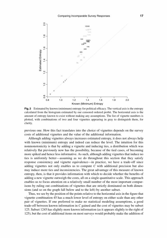
Given five vignettes on a pretest survey, we must choose among 31 possible subsets ofvignettes (where, using the labels above, these include subsets 1, 2, 3, 4, 5, 12, 13, 14, . . .,12345), excluding of course the possibility of writing new vignettes. For each of the 31choices, we computed the minimum entropy and the estimated entropy and plot the pair ina scatterplot in Fig. 2.

Figure 2 has a variety of informative features. Consider first solutions with a singlevignette, which appear in the lower left corner of the figure. Each of these appears exactlyon the 45� line where known and estimated entropy are identical. They are identicalbecause the uncertainty in estimated entropy is entirely due to ties and inconsistencies,and these are not possible with a single vignette. Substantively, we find that in these datathe vignettes with lower levels of efficacy are most informative. Indeed, in the data, 40% ofthe Chinese respondents placed themselves below vignette 1 (Moses, suffering in silence)and so are lumped together in a single category (C 5 1), and all remaining vignettes breakup the rest of the distribution. In other words, the vignettes closest to the largest number ofpeople are most informative, and in the present sample, these are the low-efficacy vi-gnettes. Adding additional vignettes, below Moses suffering in silence would be a goodidea methodologically, although convincing countries to allow these questions on publicsurveys that they must approve may be infeasible.

All subsets with greater than one vignette have higher estimated than known entropy(and thus appear above the 45� line in Fig. 2) because of the presence of ties and incon-sistencies. Overall, the figure demonstrates that adding additional vignettes always resultsin more estimated entropy. This relationship is a feature of the definition of entropy andwill always hold, although in differing degrees. In this sample, the bonus in estimatedentropy of going from one to two vignettes is a good deal larger (for all pairs other than 45)than moving from two to three, three to four, or four to five. Indeed, there appears to bea clear decreasing return to scale, as each additional vignette adds somewhat less than the


previous one. How this fact translates into the choice of vignettes depends on the surveycosts of additional vignettes and the value of the additional information.

Although adding vignettes always increases estimated entropy, it does not always helpwith known (minimum) entropy and indeed can reduce the level. The intuition for thisnonmonotonicity is that by adding a vignette and inducing ties, a distribution which wasrelatively flat previously now has the possibility, because of the tied cases, of becomingmore spiked and hence less informative. As such, although adding vignettes that induce noties is uniformly better—assuming as we do throughout this section that they satisfyresponse consistency and vignette equivalence—in practice, we have a trade-off sinceadding vignettes not only enables us to compute C with additional precision but alsomay induce more ties and inconsistencies. The great advantage of this measure of knownentropy, then, is that it provides information with which to decide whether the benefits ofadding a new vignette outweigh the costs, all on a single quantitative scale. This approachenables us to focus attention on a relatively small number of the most important compar-isons by ruling out combinations of vignettes that are strictly dominated on both dimen-sions (and so on the graph fall below and to the left) by another subset.

Thus, we see by the position of the points relative to the horizontal axis in the figure thatvignette combination 45 has a much lower level of entropy on either scale than any otherpair of vignettes. If one preferred to make no statistical modeling assumptions, a goodtrade-off between known information in C gained and the cost of vignettes may be subset125. Subset 1245 has slightly more known information (as it appears slightly to the right of125), but the cost of additional items on most surveys would probably make the addition of

0.8 1.0 1.2 1.4 1.6 1.8 2.0

0.8

1.0

1.2

1.4

1.6

1.8

2.0

Known (Minimum) Entropy

Est

imat

ed E

ntro

py

12345

123512341245

13452345

123124125134135

235234

145245

34513

1223 1415

2425

3435

45

12

3

4

5

Fig. 2 Estimated by known (minimum) entropy for political efficacy. The vertical axis is the entropycalculated from the histogram estimated by our censored ordered probit. The horizontal axis is theamount of entropy known to exist without making any assumptions. The list of vignette numbers isplotted, with combinations of two and four vignettes appearing in gray to distinguish them, forclarity.


vignette 4 not worthwhile, unless one were willing to make statistical modeling assump-tions and thus focus on estimated entropy and the vertical dimension of the figure. If wecould afford to include only four vignettes, we would not use 2345, 1345, or 1245 sincethey are dominated by 1235, 1234, or both. Out of the 10 combinations of three vignettes,123 or 125 would appear to be likely choices.

Whether to add vignettes 3 and 4 to the subset 125, then, depends on one’s trust in theordered probit modeling assumptions. These can be judged only in part by checking the fitof the ordered probit model to the untied observations. In addition, one should keep inmind that the amount gained by going from subset 125 to 12345 (vertically on the graph) isonly about half the entropy gained by going from one vignette to three. So if one can affordthree vignettes, 125 would appear to be a good choice according to these criteria. Whetherto include more depends on how comfortable one is with the assumptions.

Finally, we note that the application we have been referring to here considers only thehistogram of the entire sample. If the goal of the research is to compute the density ofpolitical efficacy in each country separately or of some causal effect, one should evaluatethese quantities directly, in a fashion directly analogous to the analysis we performed here.

5.2 Health

In order to illustrate different features of entropy results, we now conduct the sameanalysis for two different variables. Both are components of health with self-assessmentsand vignettes asked as part of the 2002 World Health Survey (conducted by the WorldHealth Organization) in a different survey in China.

We begin with an analysis of vignettes about the quality of sleep and restfulness duringthe day. For example, one of the five vignettes asked is

[Noemi] falls asleep easily at night, but two nights a week she wakes up in the middle of the night

and cannot go back to sleep for the rest of the night.

(the others can be found at the anchoring vignettes Web site), with survey question

In the last 30 days, how much of a problem did you have [does ‘‘name’’ have] due to not feeling

rested and refreshed during the day? (1) None, (2) Mild, (3) Moderate, (4) Severe, (5) Extreme/

Cannot Do.

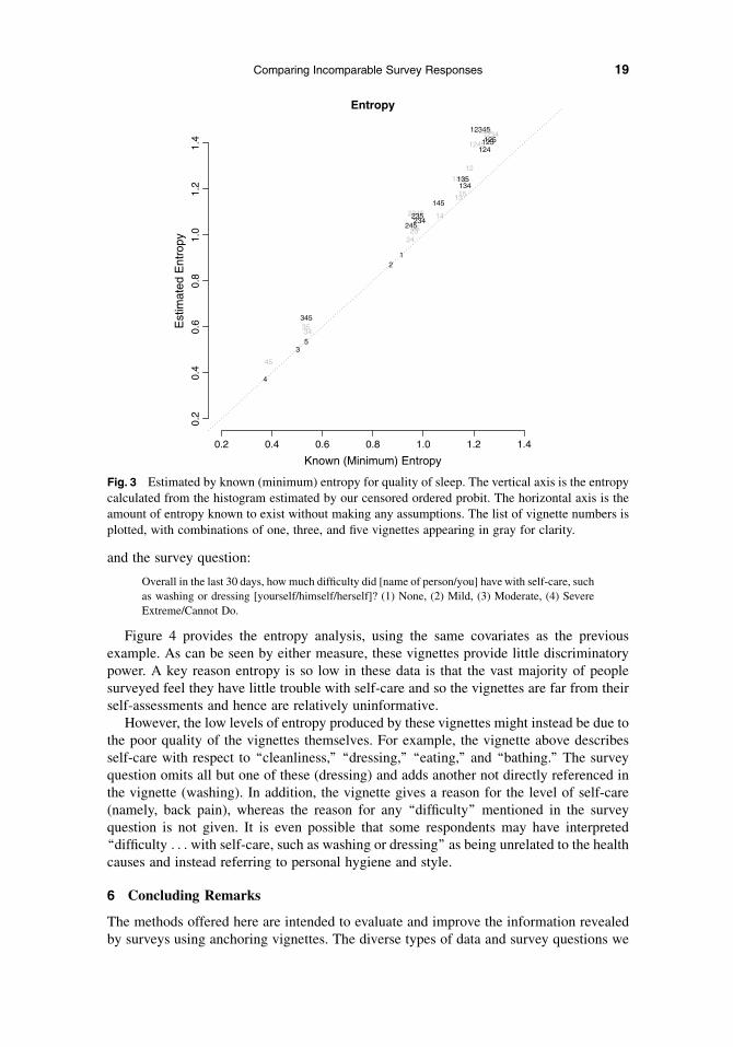
Figure 3 analyzes these data with an entropy graph in a form directly parallel to that inFig. 2.8 A particularly interesting feature of this graph is that it gives several examples ofa single strategically placed vignette providing more information than a set of threeapparently less-well-placed vignettes. In particular, either vignette 1 or 2 alone providesmore discriminatory power than vignettes 3, 4, and 5 do taken together. Indeed, this is truewhether we measure discriminatory power by either estimated or known entropy. Simi-larly, a combination of two vignettes (1 and 2) provide as much or more information thantwo sets with four vignettes (1345 and 2345) and many with three vignettes.

Finally, we offer an analysis of the self-care, with a representative vignette:

[Victor] usually requires no assistance with cleanliness, dressing and eating. He occasionally

suffers from back pain and when this happens he needs help with bathing and dressing.

8The estimated entropy for the sleep questions are calculated from the conditional fitted probabilities of a censoredprobit model with covariates sex, age, weight, years of schooling, and marital status. The same holds for self-careability, subsequently, except that height is excluded from the set of covariates since it’s inclusion leads to anunidentified cutpoint. No country dummy is included because figures are for China only.


and the survey question:

Overall in the last 30 days, how much difficulty did [name of person/you] have with self-care, such

as washing or dressing [yourself/himself/herself]? (1) None, (2) Mild, (3) Moderate, (4) Severe

Extreme/Cannot Do.

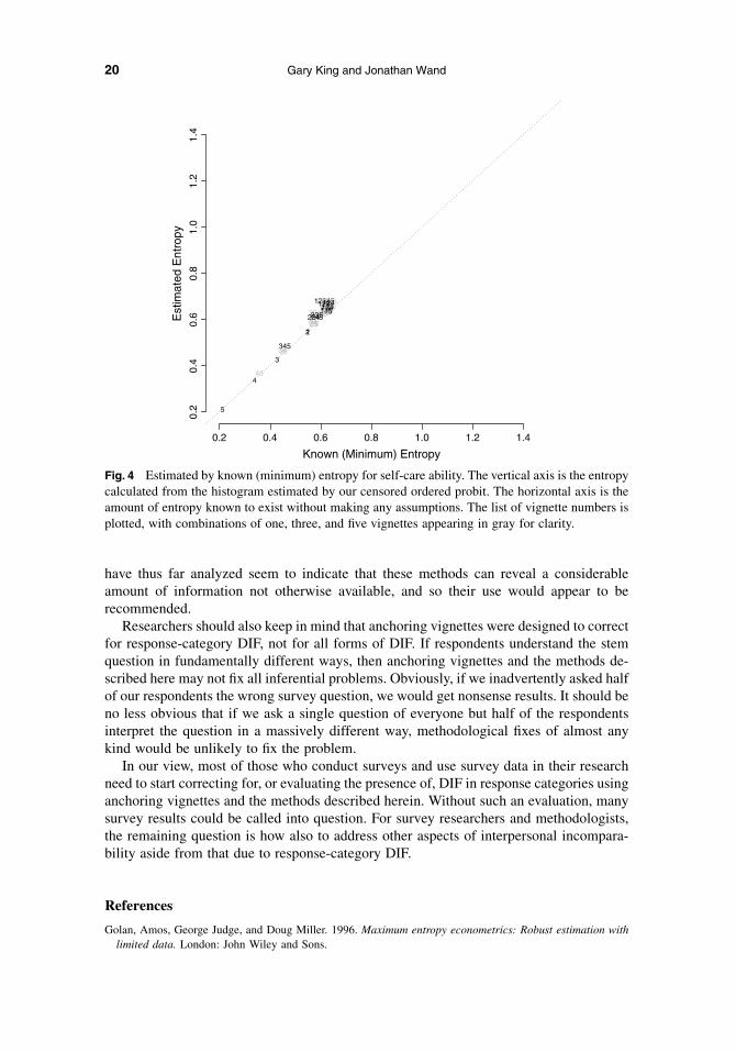
Figure 4 provides the entropy analysis, using the same covariates as the previousexample. As can be seen by either measure, these vignettes provide little discriminatorypower. A key reason entropy is so low in these data is that the vast majority of peoplesurveyed feel they have little trouble with self-care and so the vignettes are far from theirself-assessments and hence are relatively uninformative.

However, the low levels of entropy produced by these vignettes might instead be due tothe poor quality of the vignettes themselves. For example, the vignette above describesself-care with respect to ‘‘cleanliness,’’ ‘‘dressing,’’ ‘‘eating,’’ and ‘‘bathing.’’ The surveyquestion omits all but one of these (dressing) and adds another not directly referenced inthe vignette (washing). In addition, the vignette gives a reason for the level of self-care(namely, back pain), whereas the reason for any ‘‘difficulty’’ mentioned in the surveyquestion is not given. It is even possible that some respondents may have interpreted‘‘difficulty . . . with self-care, such as washing or dressing’’ as being unrelated to the healthcauses and instead referring to personal hygiene and style.

6 Concluding Remarks

The methods offered here are intended to evaluate and improve the information revealedby surveys using anchoring vignettes. The diverse types of data and survey questions we

0.2 0.4 0.6 0.8 1.0 1.2 1.4

0.2

0.4

0.6

0.8

1.0

1.2

1.4

Entropy


Est

imat

ed E

ntro

py

12345123512341251231245

124

12

13451351341513

1452345 14235

234245252324

12

34535345

3

45

4

Fig. 3 Estimated by known (minimum) entropy for quality of sleep. The vertical axis is the entropycalculated from the histogram estimated by our censored ordered probit. The horizontal axis is theamount of entropy known to exist without making any assumptions. The list of vignette numbers isplotted, with combinations of one, three, and five vignettes appearing in gray for clarity.


have thus far analyzed seem to indicate that these methods can reveal a considerableamount of information not otherwise available, and so their use would appear to berecommended.

Researchers should also keep in mind that anchoring vignettes were designed to correctfor response-category DIF, not for all forms of DIF. If respondents understand the stemquestion in fundamentally different ways, then anchoring vignettes and the methods de-scribed here may not fix all inferential problems. Obviously, if we inadvertently asked halfof our respondents the wrong survey question, we would get nonsense results. It should beno less obvious that if we ask a single question of everyone but half of the respondentsinterpret the question in a massively different way, methodological fixes of almost anykind would be unlikely to fix the problem.

In our view, most of those who conduct surveys and use survey data in their researchneed to start correcting for, or evaluating the presence of, DIF in response categories usinganchoring vignettes and the methods described herein. Without such an evaluation, manysurvey results could be called into question. For survey researchers and methodologists,the remaining question is how also to address other aspects of interpersonal incompara-bility aside from that due to response-category DIF.

References

Golan, Amos, George Judge, and Doug Miller. 1996. Maximum entropy econometrics: Robust estimation with

limited data. London: John Wiley and Sons.

0.2 0.4 0.6 0.8 1.0 1.2 1.4

0.2

0.4

0.6

0.8

1.0

1.2

1.4


Est

imat

ed E

ntro

py

12345123512451234124123125134513412135145234514132352452342324152521

34534353

454

5

Fig. 4 Estimated by known (minimum) entropy for self-care ability. The vertical axis is the entropycalculated from the histogram estimated by our censored ordered probit. The horizontal axis is theamount of entropy known to exist without making any assumptions. The list of vignette numbers isplotted, with combinations of one, three, and five vignettes appearing in gray for clarity.


Grendar, M., Jr., and M. Grendar. 2003. Maximum probability/entropy translating of contiguous categorical

observations into frequencies. Working paper, Institute of Mathematics and Computer Science, Mathematical

Institute of Slovak Academy of Sciences, Banska Bystrica.

Heitjan, Daniel F., and Donald Rubin. 1990. Inference from coarse data via multiple imputation with application

to age heaping. Journal of the American Statistical Association 85:304–14.

King, Gary. 1997. A solution to the ecological inference problem: Reconstructing individual behavior from

aggregate data. Princeton, NJ: Princeton University Press.

King, Gary, James Honaker, Anne Joseph, and Kenneth Scheve. 2001. Analyzing incomplete political science

data: An alternative algorithm for multiple imputation. American Political Science Review 95 (March): 49–69.

http://gking.harvard.edu/files/abs/evil-abs.shtml.

King, Gary, Christopher J. L. Murray, Joshua A. Salomon, and Ajay Tandon. 2004. Enhancing the validity and

cross-cultural comparability of measurement in survey research. American Political Science Review 98

(February): 191–205. http://gking.harvard.edu/files/abs/vign-abs.shtml.

King, Gary, Michael Tomz, and Jason Wittenberg. 2000. Making the most of statistical analyses: Improving

interpretation and presentation. American Journal of Political Science 44 (April): 341–55. http://gking.

harvard.edu/files/abs/making-abs.shtml.

Kullback, S., and R. A. Leibler. 1951. On information and sufficiency. Annals of Mathematical Statistics 22

(March): 79–86.

Lin, Shin, David L. Cutler, Michael E. Zwick, and Aravinda Chakravarti. 2002. Haplotype inference in random

population samples. American Journal of Human Genetics 71:1129–37.

Schwarz, Norbert. 1999. Self-reports: How the questions shape the answers. American Psychologist 54:93–105.

Sekhon, Jasjeet Singh, and Walter R. Mebane, Jr. 1998. Genetic optimization using derivatives: Theory and

application to nonlinear model. Political Analysis 7:187–210.

Shannon, Claude E. 1949. The mathematical theory of communication. Urbana-Champaign, IL: University of

Illinois Press.

Wand, Jonathan, Gary King, and Olivia Lau. Forthcoming. Anchors: Software for anchoring vignettes data.

Journal of Statistical Software.


comparing incomparable survey responses: evaluating and ... · comparing incomparable survey...

Documents