comparing error estimators for runge-kutta methods...error estimators for runge-kutta methods 447...

MATHEMATICS OF COMPUTATION, VOLUME 25, NUMBER 115, JULY, 1971

Comparing Error Estimators for Runge-Kutta Methods

By L. F. Shampine and H. A. Watts*

Abstract. A way is proposed to compare local error estimators. This is applied to the

major estimators for fourth-order Runge-Kutta procedures. An estimator which leads to

a production code 18% more efficient than a code using the standard one is recommended

and supported by numerical tests.

1. Introduction. The design of a production code for the numerical solution of

ordinary differential equations requires three major choices (at least): the method of

advancing the solution one step, the method of estimating the local error incurred in

one step, and the strategy for choosing the next step length. The first choice has been

intensively studied in the literature of numerical analysis but the latter two have been

rather neglected in spite of their great practical significance. The aim of this paper is

to compare alternatives for estimating the local error. We restrict ourselves to estima-

tors appropriate to fourth-order Runge-Kutta methods for two reasons. Production

codes based on fourth-order Runge-Kutta processes are quite common and we are

able to recommend improvements based on this study. Secondly, texts frequently

mention how easy it is to change the step size when using Runge-Kutta procedures

but they often fail to point out the associated practical disadvantages. Namely, it is

rather difficult and expensive to estimate the local error and so decide when to change

the step size. Furthermore, the standard estimator forces one to use a relatively

crude step size strategy. It is, therefore, important to consider the reliability and

efficiency of error estimating schemes.

In Section 2, we shall propose a way of comparing numerically local error estima-

tors which seems to be of broad applicability. Section 3 describes the most useful

error estimators known to the authors, which are then compared in the fourth section.

On the basis of this comparison and other facts presented, we recommend a Runge-

Kutta process using an estimator different from the standard one. To further support

this recommendation, we describe in Section 5 the results of numerical tests compar-

ing a production code using the standard estimator and the same code modified to

use the estimator we suggest.

2. Comparing Methods for Estimating Local Errors. To study numerically the

relative effectiveness of local error estimators, we shall need a broad class of dif-

ferential equations for which we can evaluate the true solution for arbitrary initial

conditions. Since the local error of Runge-Kutta (R-K) methods depends on the

form of the equation as well as the solution, it is necessary to use a variety of non-

Received November 13, 1970, revised January 21, 1971.

AMS 1969 subject classifications. Primary 6561, 6580.

Key words and phrases. Local error, error estimators, Runge-Kutta methods, step size adjustment,

solution of differential equations.

* This was partially supported by the U. S. Atomic Energy Commission.

Copyright © 1971, American Mathematical Society

445

License or copyright restrictions may apply to redistribution; see http://www.ams.org/journal-terms-of-use

446 L. F. SHAMPINE AND H. A. WATTS

linear equations. Although the class we suggest can be treated for systems of equa-

tions, we restrict our attention to a single equation

y'(x) = f(x, y(x)), y(x0) = y0.

We suggest using the class of problems defined by those / which can be represented

by a convergent double power series near the point of interest (x0, ya)- Without loss

of generality, we shall assume that (jc0, y0) = (0, 0), so that the initial-value problem

becomes

(1) y'(x) = ¿ a,,*4/' = /(*, y), y(0) = 0.i.i-0

The differential equation then has a unique solution analytic in some neighborhood

of the origin and can be represented by a power series there,

(2) y(x) = J^ctx".k-l

The coefficients can be derived recursively as follows: Define ck,¡ as the coefficient of

xk in the jth power of y,

\y(x)Y = £ ck.iXk.k-l

Noting that ck.¡ = 0 for k < j and that ckA = ck we easily obtain

*-,■

(3) ckii + i = Xc»c*-".< ÍOT J = !•n-l

On substituting these series in (1) and equating coefficients, we get

k-2 lk-1-i \

(4) kck = fli-Lo + X ( X) BiA-1-í./j ÍOT k è 1,

where we take ^¡j"1 = 0.

For our numerical studies we, of course, truncate the series (1), (2) but we still

need to know the region of convergence. Let us suppose that the ati satisfy |a,,| ^ 1.

(We shall, in fact, generate the a,, randomly and uniformly distributed in the interval

[—1, 1].) The method of majorants then guarantees that the series (2) has a radius

of convergence of at least 1 - exp(-J) = 0.3935 [1, pp. 282-283].

Let us now describe a way of comparing local error estimators. By definition, the

actual error incurred in a single step of length h, say from x = 0 to x = h, is

(5) r(h) = true local error = yh — y(h),

where yh denotes the approximate solution given by the numerical procedure. For

a method of order/), the local error is, by definition, 0(hp+1). We further assume that

for this single step

(6) r(h) = chp+1 + ahv+2 + 0(h"*3),

where c and a are constants (depending on / but independent of h). A scheme for

estimating this local error ought to be asymptotically correct; that is, the estimated

local error, e(h), should satisfy


ERROR ESTIMATORS FOR RUNGE-KUTTA METHODS 447

(7) lim ——- = p,hô r(h)

where p is a finite constant equal to one for those problems with cÔ. We shall only

consider such procedures; so let us write

(8) t(h) = chv+1 + bhv+2 + 0(hp+3),

where b is a constant (depending on /, independent of h). We shall now discuss how

we may compare estimators for sufficiently small h. For this asymptotic comparison

we compute

ra\ j/n i- e(h)—_j(h)(9) d(f) = lira-7ÍT2- = b — a.

hô n

It may seem unlikely that one would consider estimators which are not asymptotically

correct. Nevertheless, in the next section, we shall mention two such estimators. An

important point to be kept in mind is that one might base his error control on a

quantity other than local error. For example, the global error is really the quantity

of interest though this option seems almost unexplored. However, granted that one

estimates local error and that his estimator is at least asymptotically correct, it seems

reasonable to compare estimators by their effectiveness in estimating the next term

in the asymptotic expression for the local error.

Computationally, we proceed as follows: For a given problem (1), where the

a4i are generated randomly in the interval [—1, 1], we compute e and t for a sequence

of A values for each method being tested. This sequence consists of h values decreasing

to zero with the initial (largest) h chosen so that the series (2) is convergent for x —

±2h. Since we approximate asymptotic results (h —> 0), the series converges very

rapidly. Now, for each /; of this sequence, we compute the ratio in (9), until suc-

cessive approximations to d(j) differ by less than a prescribed amount. Finally, we

compute the average and maximum values of our approximations to \d(f)\ over an

ensemble of randomly chosen problems for each method.

3. Some Error Estimating Schemes. We shall first describe two estimators

which we shall not study and explain why. The Merson process [2] is used in a number

of codes. However, it does not seem to be adequately appreciated that the justification

of this method is restricted to equations of the form f(x, y) = ax + ßy + y. The

method is not asymptotically correct for general nonlinear equations, as the simple

example y'(x) = x + xy(x), y(0) = 0 shows clearly. A little computation results in

r(h) = =± h" + 0(h%),

whereas Merson's estimator gives

t(h) = ^ h/ + 0(h&),

so that Eq. (7) fails to be satisfied. Since the method is without theoretical support

for general equations, we recommend it be abandoned. It is worth comment that

although asymptotically the estimate bears no useful relationship to the true error,



codes based on it are too conservative in the choice of step size as the order of the

error is estimated to be too low. Thus, they are simply inefficient.

Zonneveld [3] gives an error estimation scheme which cannot be compared using

the method of the previous section, because he does not estimate the local truncation

error. He estimates the last term of the Taylor expansion that has been taken into

account. For a fourth-order process, this is the contribution of order /z4 which enters

into the value of yh. His numerical results seem quite satisfactory though his step

size strategy may compensate for any shortcomings of the error estimator. Hull

[4] reports some limited comparison with the doubling procedure we shall now

describe.

Extrapolation procedures are the most familiar and widely used techniques for

estimating local errors associated with Runge-Kutta methods. These compute solu-

tions (locally) twice with different step sizes and combine the results to estimate the

error in one of the values. The most common choice is to compute y2h by two steps

of length h and y2*h by one step of length 2h. The average of the error accumulated

in the two steps is then estimated by

(10) e(h) = yîh ~ y2h

for a fourth-order R-K method. This procedure will be referred to as doubling and

it seems fair to describe it as the standard estimator for R-K methods. The technique

is not limited to fourth-order processes nor to one-step methods. Theoretical details

and justification may be found in [5, pp. 80-82]. If the estimated error is acceptable,

we expend 5| function evaluations per step using any of the standard fourth-order

R-K processes. If the estimated error is unacceptable, we reduce h to A/2 so that

some of the data computed may be reused. Then, an unacceptable error results in a

loss of seven function evaluations before we recycle the computations. Although this

may not be the most efficient refinement logic with respect to number of function

evaluations per unit increase in x, such strategy seems to be universally used in

production codes.

The next class of methods we shall consider may be referred to as multistage

error estimates which are based on approximate quadrature and local expansions

at several neighboring points. Estimates of this type may be found in [6] and again

do not depend on any particular R-K process. Let us note that the error is being

averaged over several steps and may be unreliable when the error is changing rapidly.

A further disadvantage is that one now has the complications associated with the

construction of a multistep code. We shall be concerned with four such estimates.

The most accurate formula listed by Ceschino and Kuntzmann is of the form

(11) e(A) = ¿ÜLVn.i + 27.yn - 27>>B_I - llj>„-2) ~ Jj(/»+i + 9/„ + 9/»., + /„_2).

One can obtain such a formula via the Hermite interpolating polynomial. Theoretical

justification of its use is rather complicated and only sketched in [6, pp. 248-249].

A detailed derivation shows this formula to be more accurate (as applied to

methods of order g 4) when the estimated error is taken to be the error in going

from xn_! to xn. In the context of our numerical comparison scheme (recall we are



interested in the error incurred in going from x = 0 to x = h), Eq. (11) becomes

(12) e(h) = ¿j (Uy2h + 21yh - \\y.h) - |¡ (f2h + 9fh + 9/0 + /_„),

using the initial condition y0 = 0.

Here y2h, yh and >>_„ are taken to be the numerical solutions obtained from the

R-K process at the points x = 2/z, h, —h, respectively, where y^h results from an

integration proceeding backward one step from x = 0 and y2h is the two-step solution

as discussed in the doubling procedure. This way of supplying the needed data for

the error formula seems best for an unbiased comparison of the various estimators.

Now, utilizing some fourth-order R-K process in a numerical algorithm with (11)

being applied for estimating the error over xn_x to xn, we expend four function

evaluations per step as long as the error is tolerable (since we can reuse /„+1 as /„ in

the next step). If not, and our acceptability criterion calls for a reduction in step,

we lose eight function evaluations and must fill in new values for yn_2 and /n_2 which

are needed in the estimator. These would be obtained most cheaply via interpolation.

An advantage over doubling in the step size strategy is that no additional penalties

are incurred in reducing the step to other than h/2.

Alternatively, if we wish to interpret the multistage error estimate (11) as repre-

senting the error over xn to x„+x, the equation for the comparison scheme becomes

(13) e(Ä) = ¿ (Uyh - 21y-h - l\y-2h) - |j (Jk + 9/„ + 9/_» + /_»).

As before, the values y_h and y_ih are computed solutions obtained via the R-K

process by backward integration of one and two steps, respectively. Again, this way

of supplying the required values is merely for our comparison purposes, the intent

being to approximate the solution errors introduced in a normal application of the

estimator (11). The advantage of such a numerical algorithm is that one obtains an

estimate of the error incurred over the single step in which the solution is being

advanced, thereby resulting in a loss of only four function evaluations when the

current step is rejected. Again, let us assume that the missing values required for the

estimator are to be supplied by interpolation. We find that reducing the step to h/2

requires new values for yn_i and /„_i whereas reduction to other than h/2 requires

the additional values yn_2 and /„_2.

We initially included two other multistage formulas in our comparisons. These

were

(14) e(A) = ± (33jn+1 + 24.y„ - 57>-„-i) - ¿ (10/.+ , + 57/n + 24/_, - /„_,)

and

(15) e(A) = ^ (yn+i + 18^„ - 9yn.1 - \0yn_2) - ^ (9/„ + \%jn_i + 3/„_2),

formulas V*(a) and V of [6, p. 250], respectively. (Formula (15) was first given by

Morel [7].) Although Morel's estimator was more accurate than (14), they were

both found to be considerably less accurate on the average than were (12) and (13).

Because of this and the fact that they offer no other significant advantage (though use



of Eq. (15) in estimating the error over xn to xn+i does result in a loss of only three

function evaluations if refinement occurs), these estimators were dropped from our

final tests.

Our next estimator is not as well known as the previous methods. England [8]

has recently given some very efficient processes which use quantities calculated

during a R-K step in an "internal" error estimating formula. The particular scheme

of most appeal to us is given in Eqs. (8) and (9) of his paper and is completely com-

parable to the technique of doubling.

To get some feeling for the internal estimators, we derived a simple family for

the Euler-Cauchy second-order Runge-Kutta process:

k0 = hf(x0, v0),

ki = hf(x0 + h, y0 + k0),

yi = yo + h(ko + ki).

We begin on the second step, perform an extra function evaluation, and estimate the

error in yx :

k2 = hf(xi, y0,

k3 = hf(xi + ah, yi + ßk2),

n = ô0A;o + Mi + ô2k2 + 53k3.

The parameters a, ß, 80, Su 52, S3 are to be chosen so that y(x¡) — yi = r¡ -\- 0(/i4).

A relatively simple expansion and equating of coefficients leads to the equations

a = ß, 50 = -(5, + S2+ S3) and

ôi + Ô2 + (1 + a)ô3 = 0,

52 + (2a+ 1)03 = h

Sx + 62 + (1+ a)2Ô3 = -£.

For given a, there is a unique solution if and only if a 9a 0, — 1. The excluded cases

are not surprising since, for them, k3 does not provide a new function evaluation.

A very desirable choice is a = 1, for then

k3 = hf(xi + h, yi + k2),

y2 = yi + \(k2 + k3),

ri = (-ko - 5ki + lk2 - k3)/\2,

and if ri is tolerable, we have y2 immediately available and the error estimate is

obtained with no extra expense.

England's scheme uses a particular fourth-order R-K procedure which calculates

the first step by

ko = hf(x0, y0),

ki = hf(x0 + \h, ya + \K),

k2 = hf(x0 + \h, y0 + i(k0 + ki)),

k3 = hf(x0 + h, y0 — ki + 2k2),

yi = v0 + i(k0 + Ak2 + k3),



and starts calculating the second step in the same manner,

ft4 = hf(x0 + h, yO,

ks = hf(x0 + |A, yx + §ft4),

ko = hfixo + |A, yi + i(ft, + ks)).

Before completing this step, an extra function evaluation is made which allows us

to estimate the local error accumulated in two steps,

«« k- = W** + 2h> yo + e(-*° - 9^i + 92k2 - I21fta + 144ft4 + 6fts - 12*,)),(16)

r = M-ko + Ak2 + 17ft, - 23ft4 + 4fta - ft7).

Now, if r is tolerable, we complete the computation of the second step,

ks = hfix0 + 2h, yx - ft, + 2ft6),

-v2 = .yi + |(ft4 + 4ft6 + ftg),

and continue as before.

If the step size of h is acceptable, a total of A\ function evaluations per step are

made. If the step is to be rejected, we lose seven function evaluations. In this regard,

let us note that England's scheme is more flexible than doubling since we can reduce

h by any suitable factor without penalty. This remark is quite important to the design

of codes using optimally chosen step sizes.

Using the same notation as above, our error estimate over x = 0 to x = h is

(17) e(h) = y^ (ft0 - 4ft2 - 17ft3 + 23ft4 - 4ft6 + ft7),

where we substitute x0 = 0, y0 = 0 in the formulas leading to (16). Note that the

estimate of the local error incurred in one step is taken to be the average of the esti-

mated error over two steps, just as in doubling.

4. Numerical Comparisons. In order not to introduce possible extraneous

effects from different R-K processes, we have performed all comparisons using the

R-K process of England's scheme. In point of fact, while one method might perform

considerably better than another on a chosen equation, all the common fourth-order

R-K processes perform about the same on the average with perhaps a slight advantage

given to those with "optimal" parameters. However, it seems more appropriate to

our aim of comparing estimators to use the same Runge-Kutta method in all cases.

The results we give are obtained from the error estimates of Eqs. (10), (12), (13) and

(17).Let us comment further about the actual numerical experiments. All computations

were performed on a CDC 6600 computer using double precision in nearly all cal-

culations. (A double-precision word constitutes approximately 29 decimal digits.)

The statistics have been accumulated over a set of 500 problems in which twenty

terms were carried in the series (1), (2). Final results were actually obtained by averag-

ing the statistics from five different sets of 100 problems each. Since the approximate

d(f) values for the different problem sets were in good agreement and all data yielded

consistent interpretations, we were satisfied that our ensemble formed a large enough

sample to extract meaningful statistics.



We chose {h = 2~N; N = 3, A, ■ ■ ■ , 16} for our sequence of A values and accepted

"convergence" of the d(f) values if for two successive A's they agreed within 2.5

percent. (To collect additional data we actually forced a minimum of ten such itera-

tions to take place.) Usually, the convergence criterion was satisfied at this stage,

though about 10 percent of the problems did not produce "converged" d(f) values.

A detailed study of these problems indicated that the computations were being

limited by the precision available so that the results could not be improved by con-

sidering smaller values of h. These may be described as "easy" problems in the sense

that one or more of the estimators seemed to produce a d(f) value which was at least

an order of magnitude less than the corresponding average value obtained. In any

attempt to compute asymptotic limits of differences, it is implicitly necessary to

meet the convergence test before all significance is lost in the computer word. The

long word length we used makes the situation infrequent but to avoid meaningless

results, it was necessary to reject and replace by other random problems those prob-

lems for which significant values could not be obtained in this precision. Also, since

the estimator (12) generally produced values of d(f) which were smaller than the

others by roughly a factor of ten, we decided to relax the acceptance criterion for it

to 5 percent. The net effect of this discussion is that about 8 percent of the 500 problem

ensemble were replaced by other random problems not causing any convergence

difficulties. Table 1 gives the asymptotic results thus compiled. For easy recognition,

we refer to estimators (10) as doubling, (12) as C-K#l, (13) as C-K#2, and (17) as

England.

Table 1. Asymptotic Comparisons

average \d(f)\ maximum \d(f)\

C-K#l .0024 .016England .019 .11

Doubling .019 .12

C-K#2 .037 .23

Thus, asymptotically, the Ceschino-Kuntzmann estimator (12) is the most accurate

since it obtains the best agreement with the error term of order A6. In nearly all problem

rejections due to limiting precision this formula was the major cause. That is, one

could argue that the average given above is somewhat conservative relative to the

other three estimators. An important conclusion is that asymptotically the doubling

and England estimators have virtually identical behavior.

While we recognize that it is difficult to obtain meaningful results about non-

asymptotic behavior (there is a strong problem dependence here), we feel that the

following statistics collected do give the reader some feeling as to the performance

of the various methods in this respect. For each A and each method, we computed

the relative discrepancies

(18) R(h) =r(h) - e(h)

r(h)



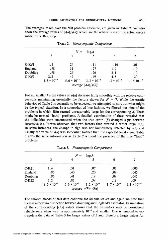
The averages, taken over the 500 problem ensemble, are given in Table 2. We also

show the average values of |t(A)/XA)| which are the relative sizes of the actual errors

made in the R-K step.

Table 2. Nonasymptotic Comparisons

N = — log2A

3 4 5 6 7

C-K#lEngland

Doubling

C-K#2

1.4.98.98

2.2.5 * 10-6 5.6

24.

31.29.49.* 10"7

average

.11

.27

.26

.493.2* 10-8

r(h)/y(h)\

.161.92.1

4.51.7* 10'

.01

.10

.10

.201.1 * 10-

For all smaller A's the values of R(h) decrease fairly smoothly with the relative com-

parisons maintaining essentially the factors shown for N = 1. While the erratic

behavior of Table 2 is generally to be expected, we attempted to sort out what might

be the typical situation. In a somewhat ad hoc fashion, we filtered out nine of the

problems in which R(h) seemed unreasonably large for the corresponding A. These

might be termed "hard" problems. A detailed examination of these revealed that

the difficulties were encountered when the true error r(h) changed signs between

successive A's. It was observed that two factors then created a rather large R(h).

In some instances, the change in sign was not immediately detected by e(h) and

usually the value of t(A) was somewhat smaller than the expected local error. Table

3 gives the same information as Table 2 without the presence of the nine "hard"

problems.

Table 3. Nonasymptotic Comparisons

N = — log2A

3 4 5 6 7

C-K#lEngland

Doubling

C-K#2

1.4.96.96

2.2

.5* HT

.31

.40

.41

.82.6 * 10"7

average

.07

.20

.19

.393.2* 10"

r(h)/y(h)\

.02

.09

.09

.181.7* KT

.006

.045

.045

.091.1* 10"

The smooth trends of this data continue for all smaller A's and again we note that

there is almost no distinction between doubling and England's estimator. Examination

of the corresponding \r/y\ values shows that the estimators may be considered

reliable only when \r/y\ is approximately 10~6 and smaller. One is tempted to ex-

trapolate the data of Table 3 for larger values of A and, therefore, larger values for



\r/y\. If this is done, the graphs of the data lead one to suspect that the estimating

procedures of doubling and England's scheme perform considerably better on a

nonasymptotic basis than do the multistage estimators. Of course, our study does

not substantiate this, but let us also recall that the estimators (12), (13) effectively

average the errors committed in three steps compared to averaging the errors over

two steps as in (10), (17). Thus, it seems plausible that large step sizes with a rapidly

changing error could conceivably result in less reliable estimates from the multistage

formulas.

We also monitored the ratios e(h)/r(h) for distinguishing features of under- and

over-estimations by the various methods. While these effects did separate the estima-

tors, the similarities were clearly evident and it was felt that no important pattern

emerged. Furthermore, we observed roughly symmetrical behavior in each estimator

with respect to under- and over-estimation by certain predetermined amounts.

5. Conclusions and Tests of a Production Code. The results of the preced-

ing section clearly show that the Ceschino-Kuntzmann estimator (12) is the most

accurate, asymptotically. However, practical considerations appear to us to make

it somewhat undesirable. The scheme partially destroys the flexibility afforded by

one-step methods and requires a relatively complicated code. To fully utilize the

good stability properties of Runge-Kutta schemes, it seems necessary to use "large"

A, but the nonasymptotic behavior of this method is questionable. Nevertheless, the

use of (12) in a code being designed should be considered since further study is

needed. The closely related estimator (11) is not competitive on the grounds of

accuracy though it is less costly.

The method of doubling and that of England are entirely comparable. Both

estimate precisely the same quantity—the error over two steps—and their accuracies

are essentially identical. England's scheme is substantially cheaper and is more

flexible for the purposes of step adjustment. The logical structures of the doubling

estimator and England's are so similar that it is an easy matter to alter a doubling

code to use the England estimator. We recommend this be done.

To demonstrate the effect of altering a doubling code to use England's estimator,

we modified a production code [9] in this way and ran a number of tests. The code to

be modified uses the classical fourth-order R-K procedure so in fact we tested three

codes. One was the production code with doubling and the classical choice of param-

eters. Another used doubling and England's choice of parameters, and the third used

England's estimator and parameters. We attempted to modify as little code as pos-

sible when incorporating these changes. Test problems were drawn from a number of

sources and were augmented with problems for which the two integration processes

performed quite differently. Runs were made with three kinds of error criterion—

relative, absolute, and mixed—and requested error tolerances of 10"*, for k —

2, A, 6, 8, 10. In most cases, average and maximum errors were evaluated on ten

equally spaced points in the interval of integration.

Full details of the tests and the results are presented in the report [10]. The data

rather uniformly show that all three codes performed with the same accuracy on the

average and the England estimator required approximately 18 percent fewer function

evaluations than the codes using doubling. This verifies experimentally what the

function counts of Section 3 would lead us to expect.



We feel a strong case has been made for altering a doubling code to use England's

estimator. While it appears that going to a Ceschino-Kuntzmann estimator might

lead to still more efficient codes, we do not know of any numerical evidence to sub-

stantiate this. We have not yet sought to make a comparison of this kind.

Mathematics Department

University of New Mexico

Albuquerque, New Mexico 87106

Division 9422

Sandia LaboratoryAlbuquerque, New Mexico 87115

1. E. L. Ince, Ordinary Differential Equations, Dover, New York, 1956.2. J. Christiansen, "Numerical solution of ordinary simultaneous differential equations

of the 1st order using a method for automatic step change," Numer. Math., v. 14, 1970, pp.317-324.

3. J. A. Zonneveld, Automatic Numerical Integration, Math. Centre Tracts, no. 8,Mathematische Centrum, Amsterdam, 1964. MR 30 #1612.

4. T. E. Hull, The Numerical Integration of Ordinary Differential Equations, Proc. IFIPCongress 68, North-Holland, Amsterdam, 1968, pp. 131-144.

5. P. Henrici, Discrete Variable Methods In Ordinary Differential Equations, Wiley, NewYork, 1962. MR 24 #B1772.

6. F. Ceschino & J. Kuntzmann, Numerical Solution of Initial Value Problems, Dunod,Paris, 1963; English transi., Prentice-Hall, Englewood Cliffs, N.J., 1966. MR 33 #3465.

7. H. Morel, "Evaluation de l'erreur sur un pas dans la méthode de Runge-Kutta,"C. R. Acad. Sei Paris, v. 243, 1956, pp. 1999-2002. MR 18, 603.

8. R. England, "Error estimates for Runge-Kutta type solutions to systems of ordinarydifferential equations," Comput. J., v. 12, 1969/70, pp. 166-170. MR 39 #3708.

9. R. E. Jones, RUNKUT-Runge Kutta Integrator of Systems of First Order OrdinaryDifferential Equations, Report #SC-M-70-724, Sandia Laboratories, Albuquerque, New Mexico,1970.

10. L. F. Shampine & H. A. Watts, Efficient Runge-Kutta Codes, Report #SC-RR-70-615,Sandia Laboratories, Albuquerque, New Mexico, 1970. (This report is available from theauthors or Sandia Laboratory, Division 3428.)


comparing error estimators for runge-kutta methods...error estimators for runge-kutta methods 447...

Documents