Comparing Charitable Fundraising Schemes: Evidence from a Field Experiment and a Structural Model

by

Steffen Huck, University College London Imran Rasul, University College London Andrew Shephard, Princeton University

Griswold Center for Economic Policy Studies

Working Paper No. 226, March 2012

�������� ������� � ���������� ������:

�������� ���� � ��� � ���������� ��� �

��������� ���� ∗

������� ���† ����� ���� ‡ ������ ������§

���� 2012

Abstract

We present evidence from a natural field experiment designed to shed light on the efficacy

of alternative fundraising schemes. In conjunction with the Bavarian State Opera House, we

mailed 25,000 regular opera attendees a letter describing a charitable fundraising project

organized by the opera house. Recipients were randomly assigned to six treatments designed

to explore behavioral responses to fundraising schemes varying in two dimensions: (i) the

presence of a lead donor; (ii) whether and how individual donations would be matched using

the lead donation. We provide reduced form evidence from the field experiment on the causal

impact of each fundraising scheme on the extensive and intensive margins of giving. We then

develop and estimate a structural model of giving behavior that simultaneously estimates

individual responses on both margins. We utilize the structural model to predict giving

behavior in counterfactual fundraising schemes. The evidence suggests the optimal fundrais-

ing scheme is one in which the charitable organization merely announces the existence of a

significant and anonymous lead donor, and does not use the lead donation to match dona-

tions in any way, be it through linear matching, non-linear matching, threshold matching, or

some combination of the three. We conclude by discussing evidence from a follow-up field

experiment designed to probe further the question why lead donors are effective.

Keywords: charitable giving, field experiment, structural estimation.

JEL Classification: C93, D12, D64.

∗We thank Sami Berlinski, Stéphane Bonhomme, Guillermo Caruana, Syngjoo Choi, Heike Harmgart, DeanKarlan, David Lee, John List, Adam Rosen, Georg Weizsäcker, and numerous seminar participants for usefulcomments. We thank the editor, Derek Neal, and two anonymous referees for comments that have improved thepaper. We gratefully acknowledge financial support from the ESRC and ELSE. We thank all those at the MunichOpera House, Actori, and Maurice Lausberg for making this project possible. This paper has been screened toensure no confidential information is revealed. All errors remain our own.

†Department of Economics, University College London [s.huck@ucl.ac.uk].‡Department of Economics, University College London [i.rasul@ucl.ac.uk].§Department of Economics, Princeton University [ajshep@princeton.edu].

1

1 Introduction

This paper presents evidence from a large-scale natural field experiment designed to shed light on

the efficacy of alternative fundraising schemes. We study the role of lead gifts, linear and non-

linear matching schemes by presenting reduced form evidence from the experiment, and estimating

a structural model of giving to inform the optimal design of fundraising schemes. We provide new

insights and show how some standard practices among fundraisers can be improved upon.1

Much of the existing literature has focussed on responses to two forms of commonly observed

fundraising schemes–linear matching [Eckel and Grossman 2006, Karlan and List 2007, Huck

and Rasul 2011] and the provision of lead gifts [List and Lucking-Reily 2002, Potters et al. 2007,

Rondeau and List 2008, Bracha et al. 2012]. We build on this literature by enlarging the set of

fundraising schemes to encompass both commonly observed and novel schemes, and to compare

them within the same setting. Our design provides external validity to aspects of giving behavior

that have been previously documented, allows us to provide new evidence on other dimensions of

giving behavior, and sheds light on the optimal design of fundraising schemes.

Methodologically, we provide both reduced form and structural form evidence from the field

experiment on the causal impact of each fundraising scheme on: (i) the extensive margin of giving,

namely, the percentage of individuals that donate some positive amount; (ii) the intensive margin

of giving, namely, the amount donated. We then develop a structural model of giving behavior

that simultaneously estimates individual responses on the extensive and intensive margins. The

structural model exploits the experimental variation to identify the underlying set of preference

parameters consistent with behavior across the fundraising schemes. At a final stage we utilize

the model to predict giving behavior under a series of counterfactual fundraising schemes, to make

progress on understanding the optimal design of fundraising schemes.2

In conjunction with the Bavarian State Opera in Munich, in June 2006, we mailed 25,000

opera attendees a letter describing a charitable fundraising project organized by the opera house.

Our natural field experiment allows us to implement various fundraising schemes in a natural and

straightforward way, holding everything else constant. Individuals were randomly assigned to one

of six treatments designed to explore behavioral responses to–(i) the presence of a substantial

lead donor, which may act as a signal of project quality [Vesterlund 2003, Andreoni 2006b]; (ii)

linear matching schemes where contributions were matched at either 50% or 100%, analogous to

considerable reductions in the relative price of charitable giving vis-à-vis own consumption; (iii)

non-linear matching schemes, where contributions above a fixed threshold would be matched at a

given rate; (iv) fixed gift matching schemes, in which any positive donation would be matched by

a fixed amount. The design of the field experiment allows us to compare behavior under commonly

1Andreoni [2006a] presents evidence from the US that in 1995, 70% of households made some charitable donationwith an average donation of over $1000, or 2.2% of household income. List and Price [2012] provide evidence thatin 2003, $241billion was given in the US, corresponding to 2% of GDP, three quarters of which stemmed fromindividuals.

2With the exception of DellaVigna et al. [2011] who study whether altruism and social pressure explain givingbehavior, there are few papers in the economics of charitable giving that combine field experimental with structuralestimation of preference parameters.

2

observed fundraising schemes that involve a lead donor or linear match rates, to less commonly

observed schemes involving non-linear or fixed gift matching.

Our main results from the reduced form analysis are as follows. First, despite their ubiquity in

fundraising campaigns, linear matching schemes do not pay for the fundraiser. As shown in Huck

and Rasul [2011], as the charitable good becomes cheaper vis-à-vis own consumption, individuals

demand more of it in terms of donations received including the match, but spend less on it

themselves in terms of donations given prior to the match. In other words, linear matching leads

to partial crowding out of the donations actually received, therefore reducing the revenues raised.

Second, potential donors are quantitatively most sensitive to the presence of a lead donor.

Relative to a control group in which no information on lead gifts is provided, donations given

increase by 44%, with no change in overall response rates. Comparing this effect with the results

from our 100% linear matching treatment we find that individuals are quantitatively more sensitive

to lead donors than to a halving of the relative price of charitable giving for example. Given

the nature of the charitable project, which has no fixed-cost element, one explanation is that

the presence of the anonymous lead donor–who commits to provide €60,000 or around 600

times the average donation–serves as a credible signal of the project’s quality as predicted by

Vesterlund [2003]. Moreover, the effect of the signal is heterogeneous across individuals–the effect

is increasing in the amount individuals would have donated in the absence of the signal, so more

generous donors are more affected. Our design, in contrast to Karlan and List [2007] for example,

is able to identify the pure impact of such lead donors, absent any offer to use the lead donation

to match others’ donations in some way.3

Third, well-designed non-linear matching schemes that require a minimum donation before

the match rate kicks-in cause donations given to be crowded in with little or no change in the

overall proportion of recipients that donate in the first place. This effect is in line with standard

consumer theory that predicts when individuals face a non-convex budget set, those that would

give relatively little in the presence of no matching might find it optimal to choose an interior

corner solution and donate more.

Finally, the fixed gift scheme leads to the highest response rates, as expected. However, we find

that even among this targeted group of regular opera attendees, 95% make no contribution to the

project. These individuals either do not value the project at all, or, face transactions costs that

are sufficiently high to offset any warm glow they feel from giving to this particular cause [Huck

and Rasul 2010]. Furthermore, the new donations drawn in with this treatment are relatively

3This is in line with the results of Potters et al [2007] who examine the role of lead contributions in a laboratorysetting. They find support for the signaling hypothesis as modelled by Andreoni [2006b]. Karlan and List [2007]also provide field evidence of such signaling effects–they find the announcement of the availability of a matchfrom a lead donor, but no specific information on the total value available for matching, increases responses onboth extensive and intensive margins of charitable giving. Providing recipients with additional information on thevalue available for matching–ranging from $25,000 to $100,000–however had little additional effect. List andLucking-Reiley [2002] study the role of seed money on charitable giving but in their research design, seed moneyserves both as a signal of quality, and also reduces the amount that needs to be collected as the project is of adiscrete nature and has a fixed fundraising target. Their design estimates the combined effects of quality signalsand the effects of reducing the additional required donations to reach the target.

3

small in magnitude. Overall, this fundraising scheme leads to full crowding out of donations

given–individuals reduce one-for-one donations given in response to the effective income transfer

received, to leave unchanged the donation actually received by the project, and to increase own

consumption by the amount of the fixed gift. Hence such matching schemes do not pay for the

fundraiser.

We then develop and estimate a structural model of charitable giving. We assume a parametric

random quasi-linear form for preferences, in which individual preferences are defined over consump-

tion and the donation received by the charitable organization. In this baseline model, individuals

are heterogeneous with respect to their valuation of the lead donation received, and we allow for

the possibility that the presence of the lead donor alters the marginal benefit from donating. We

also allow the preference parameters to depend on individual characteristics. This parsimonious

specification provides an empirically tractable framework in which we can simultaneously estimate

behavior on the extensive and intensive margins of charitable giving.

To better exploit design features of the field experiment, we then extend the baseline model

to allow for: (i) individuals restricting their donation choice to some finite and pre-determined

discrete set; (ii) some fraction of individuals exhibiting pure warm glow preferences, so that they

derive utility from their own private consumption as well as the value of their donation given,

regardless of how this is matched; (iii) focal point influences, so that some subset of donation

amounts might be particularly prominent among individuals.

Our preferred structural model is able to closely match the empirically observed response rates,

mean donation amounts, and distribution of donations given, for the control group for whom no

matching scheme is offered, as well as for those matching schemes involving a lead donor, linear

matching, and non-linear matching. The structural model does less well in fitting responses to

the fixed gift matching scheme. The structural estimates reveal that: (i) consistent with the

descriptive evidence, characteristics indicating affinity to the opera house increase the mean value

of donations; (ii) around 34% of individuals are best characterized as having pure warm glow

preferences; (iii) individuals place particular prominence on donation amounts of €50 and €100.

At a final stage, we use our preferred structural model of giving behavior to explore the

effectiveness of alternative charitable fundraising schemes. While in principle we could consider

almost any matching scheme, we focus attention to simpler parametric forms that are more realistic

extensions of commonly observed fundraising schemes. These counterfactual exercises confirm that

the optimal fundraising scheme is one in which the charitable organization merely announces the

existence of a significant and anonymous lead donor, and does not use the lead donation to match

donations in any way, be it through linear matching, non-linear matching, threshold matching, or

some combination of the three schemes.

Taken together, our analysis provides a rich set of results that shed new light on individual

giving behavior and the optimal design of fundraising schemes, and provide avenues for future

research on the role of lead donors in charitable giving.

The paper is organized as follows. Section 2 describes the natural field experiment, and presents

a conceptual framework in which to understand behavior across the treatments. Section 3 provides

4

descriptive evidence on responses on the extensive and intensive margins of charitable giving in

each treatment. Section 4 presents the reduced form analysis of individual decisions of whether

and how much to donate in each treatment. Section 5 develops and estimates a structural model of

individual preferences that best explain giving behavior, and conducts a counterfactual prediction

exercise to shed light on the optimal fundraising scheme. Section 6 concludes with evidence from a

follow-up field experiment designed to probe further the question of why lead donors are effective,

and shows how responses to lead donors vary according to: (i) the value of the lead donation; (ii)

the anonymity of the lead donor. The Appendix provides additional results and details on the

precise format and wording of the mail out.

2 The Field Experiment

2.1 Design

In June 2006 the Bavarian State Opera organized a mail out of letters to 25,000 individuals

designed to elicit donations for a social youth project the opera was engaged in, “Stück für Stück”.

The project’s beneficiaries are children from disadvantaged families whose parents are almost surely

not among the recipients of the mail out, reducing the role for gift exchange or reciprocity in driving

donations [Falk 2007], and making the campaign similar to fundraising drives by aid charities.4

The recipients were randomly selected from the opera’s database of customers who had pur-

chased at least one ticket to attend the opera house in the year prior to the mail out. Recipients

were randomly assigned to one of six treatments. Treatments varied in two dimensions–whether

information was conveyed about the existence of an anonymous lead donor, and how individual

donations would be matched by the anonymous lead donor. The mail out letters were identical in

all treatments with the exception of one paragraph. The precise format and wording of the mail

out is provided in the Appendix.5

The control treatment, denoted T1, was such that recipients were provided no information

about the existence of a lead donor, and offered no commitment to match individual donations.

The wording of the key paragraph in the letter read as follows,

T1 (Control): This is why I would be glad if you were to support the project with your donation.

This paragraph is manipulated in the other treatments. In the second treatment, denoted

T2, recipients were informed that the project had already garnered a lead gift of €60,000. The

corresponding paragraph read as follows,

T2 (Lead Donor): A generous donor who prefers not to be named has already been enlisted. He

4The project finances small workshops and events for schoolchildren with disabilities or from disadvantagedareas. These serve as a playful introduction to the world of music and opera. It is part of the Bavarian StateOpera’s mission to preserve the operatic art form for future generations and the project is therefore a key activity.

5All letters were designed and formatted by the Bavarian State Opera’s staff, and addressed to the individualas recorded in the database of attendees. Each recipient was sent a cover letter describing the project, in whichone paragraph was randomly varied in each treatment. On the second sheet of the mail out further details on the“Stück für Stück” project were provided. Letters were signed by the General Director of the opera house, Sir PeterJonas, and were mailed on the same day–Monday 19th June 2006.

5

will support “Stück für Stück” with €60,000. Unfortunately, this is not enough to fund the project

completely which is why I would be glad if you were to support the project with your donation.

The control and lead donor treatments differ only in that in the latter recipients are informed of

the presence of a lead donor. There is no offer to match donations in any way in either treatment–

a donation of one Euro corresponds to one Euro being received for the project. A comparison of

individual behaviors over the two treatments sheds light on whether and how individuals respond

to the existence of such lead donors. The literature suggests lead donors might alter the marginal

utility of giving of others through a variety of channels, such as lead gifts serving as a signal about

the quality of the fundraising project [Vesterlund 2003], snob appeal effects [Romano and Yildirim

2001], or in the presence of increasing returns, such lead gifts eliminate an equilibrium in which

all donations are zero [Andreoni 1998].6

The next two treatments provided recipients with the same information on the presence of a

lead donor, but introduced linear matching, as is commonly observed in fundraising drives. The

first of these treatments, denoted T3, informed recipients that each donation would be matched

at a rate of 50%, so that giving one Euro would correspond to the opera receiving €1.50 for the

project. The corresponding paragraph in the mail out letter then read as follows,

T3 (50% Matching): A generous donor who prefers not to be named has already been enlisted.

He will support “Stück für Stück” with up to €60,000 by donating, for each Euro that we receive

within the next four weeks, another 50 Euro cent. In light of this unique opportunity I would be

glad if you were to support the project with your donation.

The next treatment, denoted T4, was identical to T3 except the match rate was set at 100%,

so the corresponding paragraph in the mail out letter read as follows,

T4 (100% Matching): A generous donor who prefers not to be named has already been enlisted.

He will support “Stück für Stück” with up to C=60,000 by donating, for each donation that we

receive within the next four weeks, the same amount himself. In light of this unique opportunity I

would be glad if you were to support the project with your donation.

Comparing behavior in the linear matching treatments T3 and T4 to T2 allows us to estimate

the own price elasticity of donations received, as the price of giving relative to the price of own

consumption is experimentally varied.7

To be able to later present novel evidence on optimal fundraising schemes, the final two treat-

ments introduce less commonly observed fundraising schemes. The fifth treatment presented

recipients with a non-linear, non-convex matching scheme. The letter offered a match rate of

100% conditional on the donation given being above a fixed threshold–€50. Below this threshold

the match rate was zero. This was explained in the mail out letter as follows,

6Andreoni [2006b] highlights the problem that lead donors have incentives to overstate the quality of the project.Since such deception cannot arise in equilibrium it follows that lead gifts need to be extraordinarily large to becredible signals of quality. In our study the lead gift is hundreds of times larger than the average donation.

7We note that the wording of T3 and T4 differ also in how they refer to the monetary contribution of the leaddonor: T3 states the lead donor provides “another 50 Euro cent” while T4 states that the lead donor provides the“same amount himself.” Hence a comparison between these treatments picks up a change in the relative price ofgiving plus any subtle changes induced by how such wording might be interpreted by donors.

6

T5 (Non-linear Matching): A generous donor who prefers not to be named has already been

enlisted. He will support “Stück für Stück” with up to €60,000 by donating, for each donation

above €50 that we receive within the next four weeks, the same amount himself. In light of this

unique opportunity I would be glad if you were to support the project with your donation.

Beyond allowing a comparison between common and novel fundraising schemes, this treatment

also allows us to study the role of interior corner solutions as recipients who would otherwise have

given a positive amount below €50 in treatment T4 might find it optimal to give precisely €50.

Moreover, the non-convexity might introduce a focal point for donations at €50. If such focal

points influence behavior, then recipients who would have otherwise given at least €50 under

treatment T4, might be induced to reduce their donation given towards €50 under T5. The

structural estimation presented later will account for such focal point influences on behavior.

The final treatment offered recipients a fixed positive match of €20 for any positive donation.

This corresponds to a parallel shift out of the budget line and we refer to this as the ‘fixed gift’

treatment. It was explained in the mail out letter as follows,

T6 (Fixed Gift Matching): A generous donor who prefers not to be named has already been

enlisted. He will support “Stück für Stück” with up to €60,000 by donating, for each donation that

we receive within the next four weeks regardless of the donation amount, another €20. In light of

this unique opportunity I would be glad if you were to support the project with your donation.

As small donations have enormous leverage, this treatment allows us to bound the share of

recipients who do not value the project and would be unlikely to contribute in the presence of

small transactions costs of doing so.8

Four points are worth bearing in mind regarding the experiment. First, a key distinction

between our experimental design and that of Karlan and List [2007] is that they do not have

a treatment that isolates the pure signalling effect of a lead donor in the absence of any linear

matching. This is precisely what our lead donor treatment T2 captures. Rather they compare

their matching treatments with the equivalent of our control treatment T1 where there is no lead

gift. Our design allows us to decompose the effect of matching into an impact coming from the

presence of the lead donor, and the pure price effects of matching donations.

Second, the opera had no explicit fundraising target in mind, nor was any such target discussed

in the mail out. This is key to interpreting behavior when comparing the control and lead donor

treatments. For example, by announcing a lead donor that had committed to providing €60,000

in treatment T2, recipients may feel their individual donation is less needed. However, the mail

out makes clear that the money raised for the project is not used to finance one large event but

rather a series of several smaller events. Hence the project is of a linearly expandable nature such

8Huck and Rasul [2010] present evidence from another field experiment in this setting designed to explorewhether transactions costs exist, what form they take, and present a method to infer the proportion of recipientsaffected by them.

7

that recipients likely interpret that their marginal contributions will make a difference.9 ,10

Third, in treatments T3 to T6, recipients were told the matching schemes would be in place

for four weeks after receipt of the mail out. The deadline was not binding: over 97% of donations

were received during this time frame and the median donor gave within a week of the mail out.

Moreover, we find no evidence of differential effects on the time for donations to be received

between any treatment and the control treatment, in which no such deadline was announced.11

Finally, recipients are told the truth–the lead gift was actually provided and each matching

scheme was implemented. The value of matches was capped at €60,000 which ensured subjects

were told the truth even if the campaign was more successful than anticipated and, crucially, this

holds the commitment of the lead donor constant across treatments.

2.2 Conceptual Framework

We present a simple framework in which to think through the individual utility maximization

problem under each treatment. This makes precise what can be inferred from a comparison of

behavior across treatments in the reduced form estimates presented in Section 4. This framework

is then taken to the data using structural estimation methods in Section 5. Following standard

consumer theory, we assume individuals have complete, transitive, continuous, monotone, and

convex preferences over their private consumption, c, and the donation received by the project,

dr. The individual utility maximization problem is,

maxdr

u(c, dr) subject to c+ dg ≤ y, c, dg ≥ 0, and dr = RT (dg), (1)

where the first constraint ensures consumption can be no greater than income net of any donation

given, y−dg; the second constraint requires consumption and donations given to be non-negative;

and the third constraint denotes the matching scheme that translates donations given into those

received by the opera house in treatment T . Under linear matching treatments for example,

dr = λdg. This utility function captures the notion that potential donors care about their own

consumption and the marginal benefit their donation provides. Given the linearly expandable

nature of the project, this marginal benefit relates to dr.

Figure 1 graphs the budget sets induced by the six treatments in (y − dg, dr)-space. In the

control treatment (T1) the budget line has vertical intercept y and a slope of minus one as for

9The effects of such seed money are in general ambiguous and depend on whether individuals believe the projectis far from, or close to, its designated target, and whether these beliefs encourage or discourage donations [List andLucking-Reiley 2002]. Rondeau and List [2008] present experimental evidence on the effects of lead donations inthe presence of explicit targets.

10Although we cannot rule out with certainty that donors perceive their to be an implicit target, we note that ifrecipients have the same belief that others had donated to such an extent that the €60,000 of the lead donor wasalready exhausted and so the match scheme would no longer be in place, there should be no difference in behaviorsacross treatments T2 to T6. This hypothesis is rejected by the data.

11As recipients were drawn from the database of opera attendees, recipients might know each other. Havingknowledge of whether another opera attendee had received the mail out, and the form of the letter they received,may in principle change behavior if there are peer effects in charitable giving. We expect such effects to bequalitatively small and, indeed, the opera house received no telephone queries regarding treatment differences.

8

each Euro given by an individual, the project receives one Euro (dr = dg). The budget set is

identical under the lead donor treatment (T2) as there is no matching and so the relative price of

donations received is unchanged. However, if individuals infer the project is of high quality due to

the existence of a lead donor, the marginal benefit of giving may be altered and so affect behavior

on both the extensive and intensive margins. We empirically estimate whether the impact is to

increase or decrease donations.

In all remaining treatments individuals are, as in T2, aware of the existence of a lead donor.

Hence, in order to isolate the effect of variations in the budget set on behavior, the relevant

comparison group throughout is the lead donor treatment T2. The linear matching schemes in

treatments T3 and T4 vary the price of donations relative to own consumption so that with the

50% match rate in T3, λ = 1.5, and with the 100% match rate in T4, λ = 2. In both cases the

budget set pivots out with the same vertical intercept.

As Huck and Rasul [2011] show, comparing treatments T2, T3 and T4 provides estimates of

the own price elasticity of charitable donations received as the match rate varies. As the price of

consumption is normalized to one, if the match rate changes from λ to λ′, the relative price of

donations received, p, falls from 1

λto 1

λ′so the own price elasticity of donations received is,

ǫdr ,p =

(∆dr∆p

)/

(drp

)=

(∆dr1

λ− 1

λ′

)/

(dr1

λ

). (2)

where dr is the average donation received in the baseline treatment with match rate λ, and ∆dr

is the change in donations received as the match rate increases from λ to λ′.12 The reduced

form estimates allow us to recover the average own price elasticity among the sample donors,

or equivalently, recover this elasticity assuming all sample donors have the same elasticity. The

structural estimates allow for individuals to be heterogeneous along this dimension.

Two point predictions on this own price elasticity of donations are of note. First, if recipients are

engaged in pure donation targeting–where individuals always choose a particular dr independent

of the price of donations received–then moving from a match rate of λ to λ′ implies ∆dr = 0

and ∆dg =λ−λ′

λ′dg < 0. Hence the own price elasticity of donations received is ǫdr ,p = 0 so the

increased match rate leads to full crowding out of donations given. Second, if preferences are

characterized by pure warm glow–where individuals only care about the donation given rather

than that actually received. If the match rate then increases from λ to λ′ this leads to ∆dg = 0

and ∆dr = (λ′ − λ)dg > 0 so the own price elasticity of donations received is ǫdr ,p = −λ′

λ.13

The reduced form estimates are informative of whether, on average, behavior can be character-

ized by either special case, or equivalently, allow us to test whether all individuals have the same

12Charitable donations are tax-deductible in Germany which implies the actual price of the donation received willalways be marginally lower than assumed here. Any such differences will wash out in the treatment comparisonsdue to random assignment.

13The pure warm glow model, a special case of the preferences described in Andreoni [1990], implies donorsactually care only about their own consumption (y− dg) and their donation given (dg) but not about the donationreceived (dr). In this special case the budget sets would be materially identical for donors. However, as documentedlater, the data rejects the hypothesis that donors behave according to the pure warm glow hypothesis.

9

type of special-case preference. The structural estimates allow for heterogenous preferences, and

we consider a scenario where some fraction of individuals have pure warm glow preferences, and

estimate this fraction along with the preference parameters.

The non-linear matching scheme in treatment T5 causes recipients to face a non-convex budget

constraint that partly overlaps with those in T2 and T4. This treatment introduces kinks into the

budget line, and so can lead to an interior corner solution in the individual optimization problem.

This raises the possibility of donations given being crowded in by such schemes.

For each budget set considered, individuals may optimally locate at an exterior corner. Note

however that every individual with preferences satisfying ∂u∂dr

∣∣∣dr=0

> 0 should make a small positive

donation in the fixed gift scheme T6. This treatment should then have the highest response rates,

and allows us to bound the share of recipients for whom ∂u∂dr

∣∣∣dr=0

≯ 0 and so are unlikely to

contribute to the project in the presence of small transactions costs of doing so.14

3 Descriptive Evidence

3.1 Sample Characteristics and Treatment Assignment

Individuals that purchase a ticket are automatically placed on the opera house’s database. The

original mail out was sent to 25,000 individuals on the database. We remove non-German residents,

corporate donors, formally titled donors, and recipients to whom we cannot assign a gender–

typically couples. The working sample is then based on 22,512 individuals.

Individuals were randomly assigned to one of six treatments. Table 1 tests whether individuals

differ across treatments in the individual characteristics obtained from the opera’s database. Table

1 reports the p-values on the null hypothesis that the mean characteristics of individuals in the

treatment group are the same as in the control group T1. There are almost no significant differences

along any dimension between recipients in each treatments, so that individuals are indeed randomly

14Under the assumption that the source of income transfers does not matter–so that individuals respond in thesame way to the fixed gift of €20 in T6 from the anonymous donor as they would to an increase in their ownincome by €20, the field experiment can also shed light on expenditure and income elasticities of charitable giving,as have been previously estimated in the literature using non-experimental methods. More precisely, the operadatabase contains information on individual expenditures on opera tickets in the twelve months preceding the mailout, denoted x. Then in a comparison of treatments T6 and T2 and further assuming individuals have a fixedbudget for the opera that can be divided between attendance and charitable donations, the expenditure elasticityof donations received is,

ǫdr,x =

(∆dr∆x

)/

(drx

)=

(∆dr20

)/

(drx

),

where x denotes the annual expenditure on the opera in the baseline treatment T2, dr is the average donationreceived in treatment T2, and ∆dr is the change in donations received between T6 and T2. Moreover, treatmentsT2 and T6 can further be used to estimate the income elasticity of own consumption,

ǫc,y =

(∆(y − dg)∆y

)/

(y − dgy

)≈ 1− ∆dg

20,

where ∆dg is the change in donations given between T6 and T2, and as the budget share of donations given issmall, (y − dg/y) is approximately equal to one. If recipients retain all the additional income with no increase indonations given then ǫc,y = 1. Alternatively, if there is full crowding out of donations given then ǫc,y = 2.

10

assigned into treatments.15

Columns 1 and 2 show that there is an almost equal split of recipients across treatments, and

that close to 47% of all recipients are female. Columns 3 to 7 provide information on individuals’

attendance at the opera. This is measured by the number of tickets the individual has ordered

in the twelve months prior to the mail out, the number of separate ticket orders that were placed

over the same period, the average price paid per ticket, and the total amount spent. Individuals in

the sample typically purchase around six tickets in the year prior to the mail out in two separate

orders. The average price per ticket is just under €86 with the annual total spent on attendance

averaging over €400. We use information on the zip code of residence of individuals to identify

that 40% of recipients reside within Munich, where the opera house is located. Finally, we note

that the majority of individuals have attended the opera in the six months prior to the mail out.16

Two further points are of note. First, the number of tickets bought, the number of orders

placed, and whether or not a person lives in Munich, can proxy an individual’s affinity to the

opera. This may in turn relate to how they trade-off utility from consumption for utility from

donations received by the opera for the “Stück für Stück” project. In contrast, the average price

per ticket bought might better proxy individual income. We later exploit this information to shed

light on whether on the extensive margin, donors differ from non-donors predominantly in terms

of their affinity to the opera, or in terms of their incomes. The structural model we later estimate

also allows underlying preference parameters to vary with these observables.17

Second, recipients are not representative of the population–they attend the opera more fre-

quently than the average citizen and are likely to have higher disposable incomes. Our analysis

therefore sheds light on how such selected individuals donate towards a project that is being

directly promoted by the opera house. To the extent that other organizations target charita-

ble projects towards those with high affinity to the organization as well as those who are likely

to have high income, the results have external validity in other settings. Moreover, while the

non-representativeness of the sample may imply the observed levels of response or donations likely

overstate the response among the general population, we focus attention on differences in behavior

across treatments that purge the analysis of the common characteristics of sample individuals.

3.2 Donors and Non-Donors

Table 2 shows how donors and non-donors differ on observable characteristics. We report the

mean and standard error of each characteristic, as well as the p-value on the null hypothesis that

the characteristic is the same among donors and non-donors in the same treatment. Column 1

15The one exception is that there are slightly more females in T6 relative to T1. However we note that thereare no significant gender differences between those in T6 and T2, which forms a more natural group from which toidentify the causal effect of the specific matching scheme in T6.

16In Column 10 we report the p-value on an F-test of the joint significance of these characteristics of a regressionon the treatment dummy, where the omitted treatment category is the control group. For each comparison to thecontrol group, we do not reject the null.

17Of course, we cannot rule out the existence of ‘opera buffs’ whose expenditures on opera tickets are beyondtheir means. Insofar as such individuals exist, average ticket price might also reflect an element of affinity.

11

shows the number of donors overall and by treatment.

We see that individuals that have purchased more tickets in the year prior to the mail out,

have placed more separate orders over the same time period, and have last attended the opera

more recently are significantly more likely to donate in each and every treatment. In contrast,

the average price per ticket does not differ significantly between donors and non-donors in five out

of the six treatments. Munich residents are not more likely to respond in each treatment. As a

further check, we exploit additional information on average house rents in Munich by zip code,

measured in Euros per square meter. For the subset of recipients in Munich, Column 9 shows

that in each treatment, the house rental price between donors and non donors is not significantly

different, again suggesting that income proxies are not much correlated with behavior on the

extensive margin of giving.

Taken together these results suggest that affinity to the opera house is strongly correlated to

behavior along the extensive margin of whether to donate or not. Characteristics that more closely

proxy individual income are less correlated with giving behavior on the extensive margin.

3.3 Recipient Behavior: Extensive and Intensive Margins

Table 3 provides descriptive evidence on the extensive and intensive margins of giving, by treat-

ment. For each statistic we report its mean, its standard error in parentheses, and whether it is

significantly different from that in the control and lead donor treatments, T1 and T2 respectively.

Figure 1 provides a graphical representation of the outcomes of each treatment.

First, Column 1 shows that response rates vary from 3.5% to 4.7% across treatments, which

are almost double those in comparable large-scale natural field experiments on charitable giving

[Eckel and Grossman 2006, Karlan and List 2007].18

Second, despite there being large variations in the budget sets individuals face in treatments T1

to T5, there are no statistically significant differences in response rates. Neither the presence of a

lead donor nor changes in price significantly affect behavior along the extensive margin. However,

we note that the percentage changes in response rates are large across treatments, even if not

statistically different from each other.

As made clear earlier, treatment T6–that introduces a fixed gift and causes a parallel shift out

of the budget set for any positive donation–is the treatment that should induce the largest change

in the number of donors relative to the control group. The data supports this–the response rate

is significantly higher in T6 relative to the other treatments. However, the fact that the response

rate in T6 is 4.7% highlights that even among this targeted population, 95% of individuals cannot

be induced to donate. These individuals either do not value the project at all or must face

transactions costs that are sufficiently high to offset any warm glow they feel from giving to this

particular cause, and so optimally locate at the corner solution given by the vertical intercept in

Figure 1.19

18One explanation for the high response rates we obtain may be that the Bavarian State Opera has not previouslyengaged in fundraising activities through mail outs, nor is the practice as common in Germany as it is in the US.

19Huck and Rasul [2010] present evidence from a field experiment in this setting designed to explore whether

12

Column 2 shows that, despite the response rates being not statistically significantly different

from each other in the first four treatments, the total amounts donated vary considerably across

treatments. Among the full sample of 25,000 recipients more than €120,000 were donated, fully

exhausting the €60,000 of the lead donor. In our working sample of 22,512 individual recipients,

from a total of 922 donors, €85,900 was donated overall, which, as Column 3 shows, corresponds

to €127,039 actually raised for the project (including the value of matches), with a mean donation

given of €93.2.20

Column 4 shows the average amount given including zeroes among non-donors. This shows

that donations given are significantly higher in all treatments relative to the control group with the

exception of the fixed gift treatment. In comparing donations relative to the lead donor treatment,

we find no significant differences in amounts given (including zeroes) among all treatments, again

with the exception of the fixed gift treatment.

The remaining columns focus on statistics among donors. Column 5 shows that in the control

treatment T1, the average donation given is €74.3. In the lead donor treatment T2, this rises

significantly to €132. The near doubling of donations given can only be a response to the pres-

ence of a lead donor–the relative price of donations received by the opera house vis-à-vis own

consumption is unchanged. The result is not driven by outliers–Column 6 shows the median

donation is also significantly higher in T2 than in T1.

This suggests the marginal rate of substitution between consumption and donations received is

altered when individuals are aware of the existence of an anonymous lead donor who has already

pledged a substantial monetary amount to the project. While such a lead donor does not induce

new donors to enter, recipients who like the project to begin with like it even more when they

observe that somebody else is already strongly committed to it. We provide further reduced and

structural form evidence on how lead donors matter later in the paper.

In terms of linear matching schemes, we see that as the relative price of donations received falls

moving from treatment T2 to the linear matching treatments T3 and T4, the average donation

received, dr, continues to rise. The average donation received increases to €151 in T3 with a

50% match rate, and to €185 in T4 with a 100% match rate. Importantly, as shown in Figure 1

and Column 7 of Table 3, as the match rate increases, the donations given, dg, fall. The average

donation given falls from €132 in the lead donor treatment T2 to to €101 in T3 with a 50% match

rate, and to €92.3 in T4 with a 100% match rate. Column 8 reiterates that these differences are

not driven by outliers–the median donation given is significantly lower in treatments T3 and T4

than the lead donor treatment T2.

Therefore, linear matching does not crowd in donations–rather there is partial crowding out

of donations given to an extent that, although donations received increase, they do so less than

proportionately to the fall in the relative price of the charitable good. An immediate consequence is

transactions costs exist, what form they take, and present a method to infer the proportion of recipients affectedby them. They show that absent any transactions costs, 6-7% of individuals would likely donate to this fundraisingdrive, almost double the actual observed response rates in T1-T5.

20This exceeded the expectations of the Bavarian State Opera which were that €22,000 would be donated overallon the basis of a 1% response rate and mean donation of €100.

13

that straight linear matching schemes as in treatments T3 and T4 do not pay for the fundraiser. We

conclude the charitable organization is better off simply announcing the presence of an anonymous

and significant lead gift, rather than additionally using the lead gift to match others’ donations.

We later use the structural estimates to see whether this conclusion continues to hold when we

predict how individuals would have responded to other match rates.21

The final two treatments involve non-linear matching schemes. Treatment T5 induces recipients

to face a non-convex budget set. For donations below €50 the budget line is coincident with that

of the lead donor treatment T2, for donations at or above €50 it coincides with that of the 100%

matching treatment T4. Figure 1 shows that the average outcome in terms of donations given and

received in T5 replicate almost exactly those in the 100% matching treatment T4–the average

donation received in T5 is €194, as opposed to €185 in T4, and the average donation given is

€97.9, as opposed to €92.3 in T4. To see why this is so, note that in the lead donor treatment

T2 the average donation received is €132. This suggests that the portion of the budget line in T5

that lies to the left of €100 on the x-axis of donations received is irrelevant for many recipients.

In essence, treatments T4 and T5 present the average recipient with an almost identical choice.

Hence response rates and donations should not differ markedly between the two. We later use the

structural estimates to predict what giving behavior would have been had alternative threshold

values and match rates been offered.

Finally, we compare the fixed gift treatment T6 in which recipients are informed of the existence

of a lead donor and that any positive donation will be matched with €20, and the lead donor

treatment T2 in which recipients are only informed of the existence of the lead donor. As previously

discussed, response rates are significantly higher in T6 than in T2, in line with standard consumer

theory. Theory also suggests these additional donors should be willing to contribute relatively

low amounts to the project. This is strongly supported in the data, as best illustrated in Figure

1–there is a decrease in both the donations given and received in treatment T6 relative to the

lead donor treatment T2. Column 5 of Table 3 shows the average donation received in T6 is

€89.2–relative to T2, donations given fall by significantly more than €20. This result is not

driven by outliers. Column 6 shows the median donations received is also significantly lower (by

€30) in T6 than T2. These effects remain even in Columns 7 and 8 when differences in the mean

and median amounts given are considered. It is worth noting that this decrease in donations is

largely driven by a mass point of individuals that give precisely €20 under T6. The structural

estimates developed below allow for such focal point influences on giving behavior.

4 Reduced Form Evidence

We now present reduced form evidence on the extensive and intensive margins of giving. This also

allows us to establish the robustness of the simple mean comparisons in Table 3, to probe further

21If the lead donor were to offer their gift conditional on such a matching scheme being implemented, then therelevant comparison is with treatment T1, as in Karlan and List [2007]. The fundraiser is then better off takingthe lead donation and implementing a linear matching scheme rather than not accepting the lead gift.

14

some aspects of giving behavior, and to provide a transparent comparison to much of the existing

literature using field experiments in charitable giving.

On the extensive margin of charitable giving, we estimate a probit model for whether any

donation is given or not. Whether individual i donates or not depends on the budget set she faces

as embodied in the treatment she is assigned to, Ti. We also control for individual characteristics

Xi, that include whether recipient i is female, the number of ticket orders placed in the 12 months

prior to mail out, the average price of these tickets, whether i resides in Munich, and a dummy for

whether the year of the last ticket purchase was 2006.22 We report marginal effects and calculate

robust standard errors throughout.

On the intensive margin of charitable giving, the central econometric concern is that even with

random assignment into treatments, we cannot in general make valid causal inferences conditional

on donations being positive because those that choose to donate are likely to differ from those that

choose not to donate. Table 2 already highlights the observable dimensions along which donors

differ to non donors. To address this issue we first estimate for the entire sample of recipients the

following OLS specification for the donation received by the opera house from recipient i, dri,

dri = δ1Ti + η1Xi + εi, (3)

so that dri = 0 for non donors, εi is a disturbance term and all other controls are as previously

defined. Under the assumption of no spillover effects between treatments, the parameter of interest

δ1 then measures the average treatment effect on the donation received of individual i being

assigned to treatment Ti relative to whichever is the omitted treatment.23

Inference can be made on positive donations only under the condition that E[εi|Ti,Xi,Di =

1] = 0 [Angrist 1997], so that unobserved determinants of the amount donated, conditional on

giving, treatment assignment and observable characteristics, are orthogonal to unobserved deter-

minants of the decision to donate. Under this assumption, we can estimate the treatment effects

conditional on a positive donation being made using a hurdle model that explicitly assumes the

initial decision to donate (Di = 0 or 1) may be separated from the decision of how much to

donate, namely, the choice over dr conditional on Di = 1. A simple two-tiered model for char-

itable giving has, as a first stage, the probit model described above. At the second stage, we

assume donations received are log normally distributed conditional on any donation being given

so log(dri)|(Ti, Xi, Di = 1) ∼ N(δ2Ti+η2Xi, σ2). The maximum likelihood estimator of the second

stage parameters, (δ2, η2), is the OLS estimator from the following regression,

log(dri) = δ2Ti + η2Xi + zi for dri > 0, (4)

22We also experimented with alternative controls in Xi. For example, the number of tickets bought may serve asan alternative proxy for affinity rather than the number of orders placed. However, we prefer the latter measure asthe former may be confounded by recipients attending the opera with their friends and family. The main resultsare robust to slight alterations in the controls.

23The disturbance term may in part capture determinants of charitable giving such as guilt or shame. We areimplicitly assuming that such motives do not interact with the treatments so that comparisons of the change inbehavior between treatments is informative.

15

where we calculate robust standard errors throughout [Wooldridge 2002]. For each treatment, we

therefore present both the OLS and hurdle model estimates, with the caveats associated with each

set of results. In contrast, the later structural analysis simultaneously models the decision to give

and the amount given.

In all specifications, when estimating the response to the presence of a lead donor, we compare

the data from treatments T1 and T2 where the former is the reference group; when estimating

the response to linear matching schemes we compare the data from treatments T2, T3, and T4,

where T2 is the reference group, and we include two dummies for whether recipient i is assigned

to treatment T3 or to T4; when estimating the response to the non-linear matching scheme we

compare the data from treatments T2 and T5 and from T4 and T5 where, in each case the former

is the reference group; and when estimating the response to the fixed gift scheme, we compare the

data from treatments T2 and T6 where T2 is the reference group.

4.1 Lead Donor

Comparing behavior between the control treatment T1 and the lead donor treatment T2 provides

estimates of the effect of a lead donor on the extensive and intensive margins of charitable giving.

Table 4 presents the results. Column 1 shows that, in line with the earlier descriptive evidence,

recipients are no more likely to respond in the lead donor treatment T2 than they are to respond

in the control group T1. This suggests the marginal donor does not much change in response to

being informed about the presence of a substantial lead donor. However, on the intensive margin,

Column 2 shows that recipients in the lead donor treatment T2 donate significantly more than

those in the control treatment. Conditional on donating, the hurdle model estimate confirms

this result in Column 3. The magnitude of this effect implies that donations increase by around

exp δ̂2 − 1 = 44% moving from the control group T1 to the lead donor treatment T2.24

A priori, it could certainly have been the case that the lead donor increased the number of

donors, as suggested by theories of why lead donors might matter [Andreoni 1998, Romano and

Yildirim 2001, Vesterlund 2003]. The evidence however suggests that the response rate is not

much changed relative to the control group. One explanation is that the extent to which the MRS

between consumption and donations given is affected by lead donors is an increasing function of

the amount the individual would have donated in the absence of the lead donor. In other words,

marginal donors are less affected by the lead donor than are individuals who would have donated

more even in the absence of the lead donor. As a consequence, the lead donor treatment may have

quantitatively larger effects on the intensive rather than extensive margins of giving.

24Although not the focus of our study, the coefficients on the other controls in Columns 1, 2, and 3 of Table 4show that recipients who are generally more likely to donate some positive amount, under either treatment, arethose that have–(i) placed more ticket orders in the 12 months prior to the mail out; (ii) paid a higher average priceper ticket over the same period; (ii) last attended in the opera in the six months prior to the mail out. However,the magnitude of the first two effects is relatively small, while the last effect is considerable–those that attendedthe opera more recently are 2% more likely to respond than those that have not attended recently, other thingsequal. This is a quantitatively large effect given the response rate in the treatments is 3.6%. Recipients that haveplaced more ticket orders in the 12 months prior to the mail out, and have paid a higher average price per ticketover the same period, donate significantly more regardless of whichever treatment they are assigned to.

16

To provide direct evidence on this, we use quantile regression methods to characterize changes

in the shape and spread of the conditional distribution of donations received, not just the change in

the mean as estimated in (4). We therefore estimate the following quantile regression specification

at each quantile τ ∈ [0, 1],

Quantτ (log(dri)|.) = δτT2 + ητXi for dri > 0. (5)

The parameter of interest, δτ , measures the difference at the τth conditional quantile of log

donations received between the lead donor treatment T2 and the control group.

Figure 2 graphs estimates of δτ from (5) and the associated 95% confidence interval at each

quantile when the comparison treatment is T1. This shows that the effect of the lead donor is

more pronounced on those individuals that would have given more under the control treatment.

Donations in the lowest quantiles of the conditional distribution of donations given are not much

affected by the signal, suggesting the MRS for marginal donors is not affected by the lead donor. In

contrast, more generous donors are more affected by lead donors, all else equal, causing the overall

distribution of donations given to become more dispersed as it is stretched rightward at higher

donation amounts.25 The later structural analysis estimates how the presence of a lead donor

affects the distribution of subjective valuations of the project. Consistent with these reduced form

results, we find that the lead donor changes this distribution such that the effect on giving is

primarily on the intensive margin.

4.2 Linear Matching

The remaining Columns of Table 4 consider behavioral responses to the other common fundraising

scheme considered in the field experiment: linear matching schemes. We compare responses on the

extensive and intensive margin of recipients in treatments T3, which introduces a 50% match rate,

and T4, which introduces a 100% match rate, relative to treatment T2 that involves no match

rate. In all treatments, recipients are aware of the existence of a lead donor, and so comparisons

to behavior in T2 isolate the pure price effects of the fundraising schemes.

Column 4 shows that, in line with the descriptive evidence, recipients are no more likely to

respond to either price matching treatment than to the baseline treatment, T2. On the intensive

margin, the OLS estimates in Column 5 show that relative to recipients in the lead donor treatment

T2 which involves no match rate–(i) larger donations are received in treatment T3, although this

25We find little evidence that the effect of the lead donor on individual’s propensity to donate varies by theirobservable characteristics. In particular, individuals that attend the opera more frequently or purchase moreexpensive tickets are not differentially sensitive on the extensive margin to the signal. The only robust evidenceof such heterogeneous responses to the presence of a lead donor are that men are 1% less likely to respond tothe presence of a lead donor, and women are .9% more likely to respond to such information. However there isno differential effect by gender on the intensive margin. We are unaware of other studies that document whetherwomen are more responsive to quality signals in the marketplace, or whether in the specific context of charitablegiving, women are more sensitive on the extensive margin to the presence of lead donors. As a point of comparison,we note that men and women donate similar amounts in T1–the mean donation of men (women) is €76 (€72)and the median donation for both is €50.

17

is not quite significantly different from zero at conventional levels; (ii) significantly larger donations

are received in treatment T4. These results are confirmed using the hurdle model specification in

Column 3 based only on positive donations.26

In Column 6 we also report the implied own price elasticity of donations received, ǫdr ,p. This

varies from −.534 when we consider the behavioral response in T3 vis-à-vis T2, to −1.12 when

considering T4 vis-à-vis T3. In terms of special cases, in five out of six tests these estimated own

price elasticities reject the null that average behavior is characterized by individuals having pure

warm glow preferences (ǫdr ,p = −λ′

λ) or by donation targeting (ǫdr,p = 0).

Considering donations given (excluding the match), the evidence suggests that as the match

rate increases, there is partial crowding out of donations given, even if donations received increase

on average. Hence, despite their ubiquity in fundraising campaigns, linear matching schemes harm

the fundraiser because they reduce donations given. The fundraiser would be better off simply

using a large donation as an announced lead gift, rather than using it to match donations.27

In the structural estimation below, we use the estimates from our preferred specification to

predict what giving behavior would have been observed at counterfactual match rates, in partic-

ular, at match rates coincident with Eckel and Grossman [2006] and Karlan and List [2007]. This

helps shed light on whether there exists some match rates the fundraiser would indeed be better

off using rather than just announcing the presence of a lead donor.

4.3 Non-linear Matching

We next estimate the behavioral response of recipients to the non-linear matching scheme T5 that

induces a non-convex budget set. While the natural reference group is the lead donor treatment

T2, we also use the data from the 100% linear matching treatment T4 because the budget lines

in T4 and T5 coincide for donations given greater than or equal to €50. The results are reported

in Table 5. At the foot of the each column we report p-values on the null hypothesis that the

coefficients on the T4 and T5 dummy variables are equal.

26An alternative interpretation of the results might be that recipient’s behavior is driven by the inferences theymake about the lead donor over these treatments rather than any changes in relative prices. For example, inT2 the lead donor effectively commits to provide €60,000 irrespective of the behavior of others. In T3 the leaddonor commits to providing €60,000 only if other donors provide €120,000 given the match rate. Similarly, inT4 the lead donor commits to providing €60,000 only if other donors provide €60,000. In other words, the levelof commitment of the lead donor that recipients may infer is greatest in T2, second highest in T4, and lowest inT3. Three pieces of evidence contradict such an interpretation–(i) donations received monotonically decrease intheir relative price–moving from T2 to T3 to T4; (ii) donations given fall as the strength of the commitment risesmoving from T3 to T4; (iii) in actuality, the lead donation of €60,000 was exhausted by the donations from theoriginal 25,000 mail out recipients.

27As discussed in more detail in Huck and Rasul [2011], own price elasticities of charitable giving have beenthe focus of much of the earlier literature on charitable giving. In comparison to earlier large-scale natural fieldexperiments, we note that Eckel and Grossman [2006] estimate a higher price elasticity of −1.07 as match rates varyfrom 125 to 133%. Non-experimental studies using cross sectional survey data on giving or tax returns, typicallyfind a price elasticity between −1.1 and −1.3 [Andreoni 2006a]. Panel data studies using US data on tax returnshave varied findings: Randolph [1995] finds short run elasticities to be higher than cross sectional estimates at−1.55, although Auten et al. [2002] find the reverse, with elasticities ranging from −.40 to −.61. Fack and Landais[2010] use data from France and a difference-in-difference research design and find similar price elasticities.

18

On the extensive margin, Column 1 shows that recipients are significantly more likely to

respond to the non-linear matching scheme than to the lead donor treatment T2. This is in line

with standard consumer theory, because as the budget set expands in T5 relative to T2, recipients

who found it optimal not to donate in T2 might now optimally choose the interior corner solution.

There is no evidence of response rates being higher in T5 than T4. On the intensive margin, the

OLS estimates in Column 2 of all donations show significantly larger donations are received in T4

and T5 relative to T2 on average. The hurdle model estimates in Column 3 show that conditional

on a donation being made, donations received are significantly higher in T5 than treatment T4.

The wording in which treatment T5 is described in the mail out letter might lead to dg =

€50 becoming focal in recipient’s minds. If so, then relative to T4 there ought to be bunching

in the distribution of donations given from above at dg = €50 in T5. No such bunching above

dg = €50 is predicted in the standard model of consumer choice–this segment of the budget line

is available under both T4 and T5. One extension we consider in the structural estimation in

Section 5 accounts for such focal point influences on giving behavior.28

The analysis highlights that by removing a portion of the budget set for donations given less

than €50 in T5 relative to T4, most small donors optimally move to the interior corner solution

rather than the exterior solution, while large donors are unaffected–the response rates are almost

identical in treatments T4 and T5. This is in contrast to some findings in the psychology literature,

where consumers are sometimes observed forgoing a decision altogether in the presence of an

expanded choice set [Iyengar and Lepper 2000].

These results have important implications for fundraisers. On the one hand, non-linear schemes

that demand a minimum donation before the match kicks in, have beneficial effects from the

fundraiser’s point of view in that they–(i) sway those who would have given less than the threshold

amount to increase their donation to the threshold level or incrementally above it; (ii) there are no

adverse effects on response rates, nor of focal points. On the other hand, for those that would have

donated more than the threshold amount of C=50, these donors effectively face a reduced relative

price of charitable giving, which should lead to a partial crowding out of donations as found in

the straight linear matching schemes.

The optimal fundraising scheme would balance these effects. As Table 3 shows, T5 raised less

money overall than T2 suggesting the threshold amount was not chosen optimally. This is because

most donors would have given above this threshold in any case–in T2 the mean donation given

was €132. We therefore conjecture that a higher threshold, set somewhere above this amount

would have further increased the total donations given. Hence the fundraiser might be better off

by considering sending out tailor-made letters to potential donors, where the matching thresholds

are individually adjusted on the basis of predicted donations in the absence of any matching. We

explore this further by using our structural estimates to conduct counterfactual analyses on giving

behavior in response to variations of the non-convex scheme where we alter: (i) the threshold level

at which the non-convexity occurs; (ii) match rates above and below the threshold.

28Briers et al. [2007] suggest such conditional gifts provide a reference point for expected donation levels.

19

4.4 Fixed Gift Matching

The remaining columns of Table 5 present evidence on the behavioral response of recipients to

our second novel non-linear matching scheme, the fixed gift where recipients are informed that all

donations will be matched by an additional €20. The relevant comparison is again with treatment

T2. On the extensive margin Column 4 shows that, in line with the descriptive evidence in Table

3, recipients are significantly more likely to respond to the fixed gift scheme. On the intensive

margin, Column 5 shows the value of donations received is however no different to that under

the lead donor treatment T2 that involves no matching. This result is replicated using the hurdle

model estimate in Column 6 based only on positive donations.

Column 7 estimates a specification analogous to (4) for donations given rather than received.

The result shows that donations given are significantly lower in the fixed gift treatment T6. The

magnitude of this effect suggests donations given fall by around 37% moving from the lead donor

treatment T2 to the fixed gift treatment T6. While the results suggest the fixed gift increases

the proportion of recipients that are willing to donate, for those that do, the offered match leads

individuals to reduce their donation given to such an extent that the donations actually received

by the project are reduced overall.

One issue with the comparison of these treatments is that there may be a drawing in of new

donors in T6 with very flat indifference curves. These individuals give small amounts in the fixed

gift treatment T6 and would not have given at all had they been assigned to the counterfactual

treatment T2. This issue is explored further in the structural model below.

One final remark is in order. Earlier, we have noted the optimal non-linear fundraising scheme

might offer matching that kicks in above the response an individual would have chosen in the

lead donor treatment T2. In some sense, this is precisely what the fixed gift in T6 does for those

recipients whose T2 response would have been to donate zero. From that perspective, the crowding

in of small donations in T6 vis-à-vis T2 mirrors perfectly the choice of the interior corner solution

of small donors in treatment T5 vis-à-vis T2. This again suggests that an optimal fundraising

scheme would entail tailor-made non-linear matching based on what the individual would have

offered in T2. To make progress on this front, we later use our preferred structural estimates

to conduct counterfactual analyses on giving behavior to variations of the fixed gift fundraising

schemes by altering: (i) the threshold level at which the fixed gift is enacted; (ii) the size of the

fixed gift.29

29>From Column 6 we can estimate the implied expenditure elasticity of donations received, ǫdr,x, using themethod described in Section 2. We find this to be .006, which although significantly different from zero, is aquantitatively small effect. From Column 7 we can estimate the implied income elasticity of own consumptionǫc,y–this is found to be 1.92, which is significantly different from zero and we cannot reject the null that ǫc,y = 2so there is full crowding out of donations given by the fixed €20 match. As the expenditure elasticity of donationsreceived is close to zero, this suggests that donations given are likely to have a weak, but positive, relationshipwith income. The fact that the income effect is found to be so weak in turn implies, that the observed priceeffects in treatments T3 and T4 are nearly all attributable to substitution rather than income effects. Studies usingcross sectional data have typically reported income elasticities in the range .4 to .8 [Andreoni 2006a]. Panel dataestimates include those of Randolph [1995], who finds short run income elasticities to be considerably smaller at.09. Auten et al. [2002] use a similar panel of tax payers and find short run elasticities of .29. In the field, Eckeland Grossman [2006] report a far higher income elasticity of 1.07. These estimates are in sharp contrast to our

20

5 Structural Form Evidence

5.1 Baseline Model

We now develop and estimate a structural model of charitable giving to: (i) assess the extent to

which we are able to explain giving behavior across the six treatments with a parsimonious model;

(ii) predict behavioral responses on the extensive and intensive margins of giving to a richer set

of designs of charitable matching schemes than those in the natural field experiment.

As in the conceptual framework developed earlier, in our baseline model we assume individuals

have preferences defined over their private consumption, c, and the donation received by the

project, dr. Individuals are heterogeneous with respect to their valuation of the lead donation

and this is indexed by the one dimensional parameter θ, which has the cumulative distribution

function Fθ(·;L). L = 1 denotes the presence of a lead donor (as in treatments T2—T6), with

L = 0 otherwise. This formulation therefore allows for the possibility that the presence of the lead

donor alters the marginal benefit from donating. As in the earlier analysis, we remain agnostic as

to whether this is because the lead donation provides a signal of the project quality or for some

other reason. We begin by assuming a random quasi-linear form for preferences,

u(c, dr; θ) = c+ θdr −α

2d2r, (6)

where α > 0, and with individuals subject to a budget constraint, c+ dg ≤ y, and non-negativity

constraint, dg ≥ 0. The donation received dr is related to the donation given dg through the function

dr = RT (dg) which varies with the fundraising scheme in place in treatment T . This utility

specification provides an empirically tractable framework and also permits both intensive and

extensive responses when the donation matching rate varies.30 Throughout this section we abstract

(for notational simplicity) from any dependence of the structural parameters upon observable

demographic characteristics. However, such dependence does not complicate the analysis and will

be incorporated in all our empirical specifications.31

5.1.1 Linear Matching

Under the linear matching treatments T1 to T4, dr = λTdg, where λT is the matching rate in

treatment T . The donation given is strictly positive if θλT > 1, that is, the marginal utility of

giving at dg = 0 exceeds the marginal utility of consumption. When positive, the donation given

findings, that unlike earlier studies, are based on experimental variation in income as induced by a parallel shiftout of the budget set faced by recipients in treatment T6, although this variation of €20 is of course very smallrelative to total income.

30The Constant Elasticity of Substitution specification has been used in previous work on charitable giving, suchas Andreoni and Miller [2002]. Setting u(c, dr; θ)−ρ = c−ρ + θd−ρr would not yield any change in the donation rateas the matching rate is varied. >From Table 3 we see that this pattern is clearly rejected in our data.

31The model thus allows us to take seriously the possibility of heterogeneous responses to fundraising schemes.In contrast, the bulk of the earlier literature has considered mean effects. A notable exception is Fack and Landais[2010] who use three-step censored quantile regression methods to address censoring issues related to donors beingself-selected and then explore heterogeneous responses to tax reforms in France related to charitable giving.

21

satisfies the first order condition,

dg =θλT − 1αλ2T

, (7)

so that dg is increasing in the individual’s valuation, θ. With slight abuse of our earlier notation,

we write the associated indirect utility function as,

u(y; θ, α, T ) =

y +(θλT − 1)22αλ2T

if θλT > 1;

y if θλT ≤ 1.(8)

which will be useful when examining optimal individual giving behavior in the next treatment.

5.1.2 Non-linear Matching

In the non-linear matching treatment T5, donations are matched one-for-one, but only if the

donation given is greater than €50. Thus, in order to determine the optimal choice of dg we need

to consider the utility attained from either not donating, donating exactly €50, or donating some

positive amount that is either more than or less than €50. To do so, we consider the parameter

restrictions that are consistent with the various piecewise linear sections of the budget set having

(or not) an interior solution and comparing maximized utility levels. An exhaustive description of

the optimal dg for all possible parameter values {α, θ} is provided in the Appendix. These giving

patterns are also summarized in Figure A1: the yellow area corresponds to the set of parameters

where an individual is on the matched section of the budget constraint with dg > 50; the orange

area is the parameter set where dg = 50; the brown area is the parameter set where 0 < dg < 50.

An important implication of the model under treatment T5 is that for a given α the support of

dg may not be connected, even if the support of θ is. This is because the matching structure may

induce individuals who would have donated slightly below €50 in the lead donor treatment T2,

to donate exactly €50. Moreover, for α < 1/100 donations below €50 are never optimal. These

observations suggest that further heterogeneity and/or model features may need to be incorporated

to explain actual giving behavior in this treatment. We return to this issue in Section 5.4 when

we further allow for pure warm glow and focal point influences.

5.1.3 Fixed Gifts

Under treatment T6 there is a €20 match for any strictly positive donation amount so that

dr = dg + 20. We need to consider the possibility of an individual donating: (i) identically zero;

(ii) a strictly positive (but negligible) amount; (iii) a strictly positive and non-negligible amount,

dg > 0. At an interior solution where the individual donates dg > 0, their utility is,

u(y − dg, dg + 20; θ) = y − dg + θ[dg + 20]−α

2[dg + 20]

2, (9)

22

which for dg > 0, is maximized when,

dg =θ − 1α

− 20. (10)

Thus there is 100% crowding out of donations for individuals who would donate in both T2

and T6. This stark prediction arises because of the absence of any income effects in our simple

preference specification. The model also predicts that the number of individuals who are donating

strictly positive (and non-negligible) amounts falls relative to the lead donor treatment T2. These

correspond to individuals who would have donated less than €20 in T2. It is straightforward

to verify that individuals will donate strictly positive non-negligible amounts in the fixed gift

treatment T6 if θ > 1 + 20α.

The baseline model also predicts mass of individuals donating a negligible amount to the

charitable cause. Individuals will prefer to donate this amount relative to either not donating or

donating a non-negligible amount if 10α ≤ θ ≤ 1 + 20α. Individuals do not donate if θ < 10α.

The proportion of individuals donating some negligible or non-negligible amount will therefore rise

relative to the lead donor treatment T2 provided α is not too high.

5.2 Discrete Version

Formulating the model with a continuous choice over donation amounts dg is natural and also

useful for exploring the theoretical implications of the model. However, despite the fact that over

900 individuals donate a strictly positive amount across the six treatments as Table 2 shows, the

actual data only has 30 positive points of support for donations across all treatments.32 While we

are not able to explain why individual donations are concentrated at certain amounts, a discrete

choice formulation of the model at least allows us to recognize the existence of this behavior.

We therefore also consider a discrete variant of our baseline model, where we maintain the

same underlying choice model as described above, but restrict dg to belong to some finite and

pre-determined set Dg. The theoretical implications of our baseline model with a discrete choice

set remain essentially the same as in the continuous choice version discussed above. Throughout

we assume that all K + 1 elements of Dg are ordered 0 = d0g < d1g < . . . < dKg <∞, so that there

is a range of θ consistent with the optimal choice dg = dkg for 0 < k < K. In the linear matching

treatments this is easily shown to satisfy,

1

λT+

αλT2× [dkg + dk−1g ] ≤ θ <

1

λT+

αλT2× [dkg + dk+1g ]. (11)

A very similar set of inequalities can be derived under the fixed gift treatment T6, while under

the non-linear matching treatment T5 it is again necessary to compare maximized utilities on the

32Across the full set of treatments T1—T6, three donation values account for almost 60% of all donations given;twelve donation values account for over 90% of all donations.

23

different sections of the budget constraint.33

5.3 Estimation of Baseline Model Using T1—T4

We first structurally estimate the baseline model under the alternative assumptions of continuous

and discrete choice sets, using maximum likelihood estimation in both cases. The estimation is

performed only using data from the linear matching treatments T1—T4, that replicate commonly

observed fundraising schemes, with the experimental variation in match rates permitting separate

identification of the structural parameters. These parameter estimates then allow the model to be

used for an out-of-sample prediction exercise in the remaining treatments T5 and T6, that relate

more to novel fundraising schemes.34

In the empirical implementation we specify a parametric distribution of the unobserved hetero-

geneity θ. This distribution may vary both with individual characteristics Xi, as well as exposure

to the lead donor treatment groups (L = 1). Throughout we assume this distribution is nor-

mal, with unknown mean and variance. The mean of the distributions is allowed to vary with

demographic characteristics through a linear index restriction, µLθ = X ′βLθ . We do not place any

restrictions on these relationships across L = 0 and L = 1.35 The full parameter vector of our

model is then given by {α, β0θ, β1θ, σ0θ, σ1θ}.Under the linear matching treatments we may re-write equation (7) as dr = max{0, d∗r}, where

33In particular, in T6, the range of θ consistent with the choice dg = dkg for 1 < k < K is,

1 +α

2× [dkg + dk−1g + 40] ≤ θ < 1 + α

2× [dkg + dk+1g + 40],

and with dg = d1g optimal when,

d1gd1g + 20

+α

2× [d1g + 20] ≤ θ < 1 +

α

2× [d1g + d2g + 40].

For T5, the range of θ such that dg > 50 is optimal is defined by the same set of inequalities as in equation (11)with λT = 2. For any dg < 50, the range of θ must simultaneously satisfy equation (11) with λT = 1, as well as,

θ <50− dkg100− dkg

+α

2× [100 + dg],

which is the requirement that the utility from dg < 50 strictly exceeds that from dg = 50. Note that the range ofθ consistent with a given 0 < dg < 50 being optimal may be an empty set.

34Given the simple structure of the model under treatments T1—T4 and the fact that these fundraising schemesare most commonly observed, it is convenient and natural to estimate the model on this subset of treatments toassess the out-of-sample predictive ability. We can of course also consider estimations based on an alternative subsetof treatments. To identify the parameters of Fθ(·; 0) it is always necessary to use data from T1. The parameters ofFθ(·; 1) and α can be separately identified using data only from treatment T5. Parametric identification is possiblewithout experimental variation because we are assuming that the same shape parameters (a mean and variancefrom a normal distribution) are responsible for giving behavior on both the unmatched and matched sections ofthe budget constraint. Non-parametric identification however requires experimental variation.

35The individual characteristics controlled for in Xi are whether recipient i is female, the number of ticket ordersplaced in the 12 months prior to mail out, the average price of these tickets, whether i resides in Munich, and azero-one dummy for whether the year of the last ticket purchase was 2006.

24

the latent variable d∗r is defined by,

d∗r =θ

α− 1

αλT=

X ′βLθα

− 1

αλT+

ǫ

α. (12)

The maximum likelihood estimates from the continuous choice baseline model specification can

then be obtained from two independent Tobit regressions: the first uses data from treatment T1

and regresses dr = dg on the set of individual controls Xi (including a constant); the second uses

data from T2—T4 and regresses dr = λTdg on the same set of controls Xi (including a constant)

as well as the inverse matching rate λ−1T . Of course, this equivalence will not hold if heterogeneity

is allowed to enter the model more generally, or if restrictions are imposed on the influence of

demographics across L = 1 and L = 0.

When estimating the discrete version of the model we define the choice set,

Dg = {0, 10, 20, 25, 30, 35, 50, 100, 150, 200, 350, 500, 1000}. (13)

Individuals observed donating some amount not contained within Dg are assigned to the nearest

donation amount in this set. The likelihood function here is simply comprised of the product of

the donation choice probabilities, which themselves are given by the probability that θ belongs to

the interval as defined by equation (11).36

Table A1 presents the preference parameter estimates of {α, β0θ, β1θ, σ0θ, σ1θ} from the baseline

model using data from T1—T4. Panel A shows the estimates from the continuous choice model,

and Panel B shows the estimates under the discrete version of the model. Bootstrapped standard

errors using 500 repetitions are shown in parentheses. Three points are of note. First, the pa-

rameter estimates are very similar, regardless of the assumed continuous or discrete choice set.

Second, observables that indicate affinity to the opera house (number of ticket orders placed in

the 12 months prior to mail out, whether the year of the last ticket purchase was 2006) increase

the mean valuation of donations, θ. Third, there is considerable imprecision in the parameter

estimates. Comparing the estimation results with and without the lead donor, our results suggest

that exposure to the lead donor treatments changes the distribution of valuations θ such that:

(i) fewer individuals would donate, i.e. Fθ(1; 1) > Fθ(1; 0); (ii) the proportion of individuals with

high realizations of θ (and therefore higher donations) increases.

Table 6 then shows the fit of both formulations of the model on the two key statistics related to

the extensive and intensive margins of giving behavior: the response rate, and the mean donation

given conditional on response. Columns 1 and 4 show the empirical values for each statistic.

Within sample using treatments T1—T4 that relate to commonly observed fundraising schemes,

the structural model does well in explaining both the donation rate and mean conditional donations

in T1. However, the fit in T2—T4 is much less satisfactory especially on the intensive margin. As

36Defining the supremum of the set defined in equation (11) as θk

T (α) and the infimum as θkT (α) the probability of

donating amount dkg is given by Φ([θk

T (α)− µLθ ]/σLθ)−Φ

([θkT (α)− µLθ ]/σLθ

), where Φ is the cumulative distribution

function of the standard normal distribution.

25

Columns 4 to 6 show, the estimated structural model, in either continuous or discrete choice

formulations, substantially over-predicts the mean donation given in the lead donor treatment T2,

and suggests a very steep price gradient as the matching rate increases.

The out-of-sample fit of both formulations of the model are also unsatisfactory, as shown in

the lower half of Table 6. In the non-linear matching treatment T5, the response rate is far lower

(3.3% or 3.4%) than is empirically observed (4.3%), and the average donation given are higher

than is observed.

In the fixed gift treatment T6, the baseline structural does predict the response rate to be

higher than in other treatments and matches quite closely the empirical response rate of 4.7%. On

the intensive margin of giving behavior, the baseline model performs poorly in both continuous

and discrete choice formulations. In both cases, donations given are predicted to be considerably

higher relative to what is observed. This suggests the baseline model under predicts the extent

to which under this fundraising scheme, relative to the lead donor scheme, existing donors might

reduce their donations as they are crowded out by the fixed gift.37

5.4 Extensions

The unsatisfactory empirical performance of the baseline model motivates us to explore a number

of extensions. We consider these extensions in the context of the discrete version of the model,

though most apply equally when dg is continuous. Finally, while we describe introducing each of

these extensions in isolation, they can and will be incorporated simultaneously.

5.4.1 Pure Warm Glow Preferences

We assume there exists some fraction πw of individuals who exhibit pure warm glow preferences.

Such individuals derive utility from their own private consumption as well as the value of their

donation given dg, regardless of how this is matched. They do not value any potential matching

donation given by the lead donor, dr − dg. It therefore follows that individuals with pure warm

glow preferences behave as described in the baseline model when subject to treatment T1 or T2,

and when subject to any of the matched treatments their behavior is the same as under T2.38

Allowing for pure warm glow preferences provides a mechanism through which any change in

the donation matching rate will, all else equal, generate smaller movements in donations given

and hence received. Relative to baseline model above, we would then expect responses to the

linear matching treatments to be closer to those under the lead donor treatment T2. This may

37The reason the baseline model is unable to fit T5 can be seen very clearly from Figure A1. The only way thebaseline model can increase the donation rate relative to T2 (aside from possible influences due to demographicdifferences) is if α < 1/100 (but note that in this case the model would not permit any donations below €50).Thus, given the estimated parameter values, the non-linear matching structure induces some individuals alreadydonating to increase their donation amount, but it does not induce non-donors to give.

38An alternative interpretation of this extension is that there exists a fraction πw of individuals who believethat their donation will be unmatched due to the committed €60,000 of matched funds being exhausted. Thisformulation is also similar (though not equivalent) to an expected utility maximizer, where the uncertainty concernsthe subjective probability that their donation will be matched.

26

overcome the steep price gradient documented in Table 6 from the baseline structural estimates.

Furthermore, provided θ has full support, the presence of such behavior implies that any positive

donation amount in any treatment may be rationalized.

5.4.2 Focal Points

We previously noted that actual donations are concentrated at a small number of donation values.

Even in the linear matching treatments T1—T4, the three most frequent donation amounts (€20,

€50, and €100) account for 60% of all positive donations, resulting in a multi-modal distribution

of donation amounts. While we are not able to explain why specific donation amounts display

such prominence, we incorporate them in our model by allowing individuals to be attached to

these focal donation amounts. We proceed as follows.

For each donation amount dkg we introduce an associated parameter ξk that enters the utility

function additively and therefore makes particular donation choices more or less likely,

u(c, dr; θ) = ξk + c+ θdr −α

2d2r. (14)

Since for certain parameter values, the range of valuations θ consistent with a particular donation

amount may have zero measure, we construct the following smoothed probabilities for a given

donation amount dkg , which are then used when forming the likelihood function,

Pr[dg = dkg ] =

∫

θ

exp(u(y − dkg , dkr ; θ)/ν)∑K

l=0 exp(u(y − dlg, dlr; θ)/ν)

dFθ(θ;L), (15)

so that as the smoothing parameter ν → 0 the probabilities in equation (15) converge to the

original unsmoothed choice probabilities.39

In our empirical applications we restrict ξk to be zero for all donation amounts except dg ∈{20, 50, 100}. When estimating the model using data only from T1—T4 we do not allow the

captivity parameters {ξk} to vary across treatments. Since the non-linear matching treatment T5

may be expected to strengthen focal behavior especially at dg = 50, and similarly the fixed gift

treatment T6 may strengthen it at dg = 20, we also explore the possibility of appropriate parameter

shifts when estimating the model using data from alternative treatments. This flexibility might

be especially important in allowing the model to better fit the empirical data from the novel

fundraising schemes embodied in T5 and T6.

39An alternative behavioral interpretation of the probabilities in equation (15) is that for each donation amountdg there exists an additive Type-I extreme value error attached to the utility function in equation (14), with astandard deviation that is proportional to ν. In our empirical application we set ν = 1/10.

27

5.4.3 Flexible Curvature

Our third extension allows for greater flexibility in functional form by specifying preferences as,

u(c, dr; θ) = c+ θdr −α

γdrγ, (16)

with γ > 1, and utility maximized subject to the same set of constraints as before. While this

generalization does not change the condition for donations to be positive under linear matching, it

does offer more flexibility in responses following any change in the matching rate. If dg is discrete,

then we obtain a modified set of inequalities determining optimal dg. In particular the range of θ

consistent with the optimal choice dg = dkg for 0 < k < K in treatments T1—T4 is now given by,

1

λT+

αλγ−1T

γ×[(dkg)

γ − (dk−1g )γ

dkg − dk−1g

]≤ θ <

1

λT+

αλγ−1T

γ×[(dk+1g )γ − (dkg)γ

dk+1g − dkg

]. (17)

Bounds on θ consistent with choice behavior in the other treatments can similarly be derived.

5.4.4 Estimation of Extended Models

The model fit under the alternative extended model specifications is presented in Table 7. Panel A

shows the model fit on response rates, and Panel B shows the model fit in terms of mean donation

given, conditional on some strictly positive donation. Columns 1 to 3 in both panels show that

introducing each of the extensions in isolation, results in noticeable improvements in the within

sample fit as measured by the response rate and mean conditional donation given in treatments

T1—T4. Incorporating either pure warm glow preferences (estimated for π̂w = 27% of individuals),

a flexible curvature parameter, or focal points, all provide a mechanism through which changes in

the matching rate may have a smaller impact on average donations than in the baseline model.

When considering each feature in isolation, warm glow preferences provide the best fit to mean

conditional donations, though the specifications which incorporate focal points do much better in

matching other features of the donation distribution, as discussed further below.

In terms of out-of-sample fit to treatments T5 and T6 shown in the lower half of each panel, we

continue to systematically under predict the response rate in the non-linear matching scheme T5

(3.6% versus 4.3% observed). In most extensions considered we still obtain preference parameter

estimates that leave donations unchanged relative to the lead donor treatment T2. None of the

specifications considered are capable of describing giving behavior in the fixed gift treatment T6.

This is unsurprising since the extensions considered all improved the within sample fit by making

donations less responsive to changes in the fundraising scheme in place, RT (·).Column 4 presents results from our preferred specification that combines focal points with

warm glow preferences. Panel C of Table A1 shows the estimated preference parameters from

this specification, {α, β0θ, β1θ, σ0θ, σ1θ, πw, ξ20, ξ50, ξ100}. We see that when combining warm glow and

focal point extensions, the estimated fraction of recipients with warm glow preferences rises to

π̂w = 34% of individuals. We also see that there is considerable focal attachment at dg = 50

28

and dg = 100, while ξ̂20 is not statistically different from zero. Figure 3 shows the predicted and

empirical distribution of strictly positive donation given amounts from this extended model with

both focal points and warm glow preferences. This shows that the model generally does well in

explaining the entire distribution of donations, not just the mean shown in Table 7.

However, despite the presence of focal points, the model still under predicts donations at

dg = 50 slightly across all fundraising schemes. While increasing ξ50 would increase donations

at this point, it would result in a deterioration in fit at the neighboring donation amounts. The

general shape of the distribution is also correct in the out-of-sample prediction exercise for the

non-linear matching treatment T5, although the proportion donating at dg = 50 is under predicted

which also accounts for the discrepancy response rate, where the model predicts a response rate

of 3.6% versus the empirically observed 4.3%.

The fit to treatment T6 is clearly the least satisfactory, both in terms of the mass at dg = 20

(rather than at the lowest discrete category) as well as the virtual absence of any donations actually

observed to be above €200, despite the model predicting such large donations. In summary, the

baseline and extended models are unable to explain the presence of more than complete crowding

out in the fixed gift treatment T6.

One interpretation of the model’s inability to fully match giving behavior in T6, and to a lesser

extent in T5, is that these treatments themselves strengthen individuals’ attachment to specific

donation amounts. Of course such behavior cannot be predicted out-of-sample with our model,

and so the preferred way to allow for it is to estimate the structural model using all six treatments

and allow the attachment parameters to vary with these treatments. The results of doing so are

shown in Columns 5 and 6 in Table 7. Estimating the model on treatments T1—T5, Column 5 in

each Panel shows we obtain little improvement in model fit by allowing ξk to vary. Indeed, the

estimated captivity parameters at dg = 50 are essentially the same for T5 as it is for T1—T4. By

increasing the attachment to a particular donation amount we raise the number of individuals at

that amount, but only by drawing individuals from the neighboring donation amounts. Column

6 shows that when we allow the attachment parameter ξ20 to vary with exposure to the fixed gift

treatment T6, the substantial over-prediction of average donations remains.

A natural extension of the baseline model that might help to fit T6 would be to allow income ef-

fects. While such effects are theoretically straightforward to incorporate into our analysis, our data

does not include any measures of income, and any attempts to proxy income with other measures

produces results that are very sensitive to the way in which income effects are parameterized.40

40We first explored the possibility of matching our data to external data sources on income by zipcode. Unfortu-nately, available data sets such as the German Socio-Economic Panel (for which zipcode information is collected)have insufficient sample size. We were able to collect average house price information for our sample period forthe Munich zipcodes, as shown in Table 1. Using these data we then attempted to relate an unknown paramet-ric distribution of income to this house price data and then integrating over this distribution in the likelihoodfunction. Restricting ourselves to the subsample of Munich households considerably reduced sample size. Overall,such attempts to incorporate income effects performed very poorly, with our results highly sensitive to alternativeparameterizations on how we allow for the possibility of income effects in the utility function.

29

5.5 Counterfactual Charitable Fundraising Schemes

We now use our preferred structural model of giving behavior to explore the effectiveness of

alternative charitable fundraising schemes. We conduct such counterfactual experiments using the

estimated parameters from the structural model with a discrete choice set, warm glow preferences,

and focal points.41 While in principle we could consider almost any matching scheme, we focus

attention to simpler parametric forms, that are more realistic extensions of commonly observed

fundraising schemes. The reduced form and structural form evidence presented thus far suggests

that from the fundraiser’s point of view, among the schemes considered in the field experiment,

it is optimal for the charitable organization to merely announce the existence of a significant and

anonymous lead donor, and not to use the lead donation to match donations in any way. The

aim of the counterfactual exercises performed is to explore whether there are other fundraising

schemes beyond those in our field experiments that out-perform the lead donor treatment.

Table 8 presents the findings from the various counterfactual schemes considered. As a point

of comparison, Column 1 shows the predicted outcomes from the preferred model for the lead

donor treatment T2. At the foot of each column we show the predicted response, and mean

donation given conditional on a strictly positive donation being made. Finally, because in some

of the counterfactual exercises the response rate and mean conditional donation given might move

in opposite directions, we also report the average donation given (including zeroes) to assess the

overall performance in terms of revenue raised of each fundraising scheme.

5.5.1 Linear Matching Schemes: Higher Match Rates

We first use our structural model to predict how revenue raised varies with linear matching rates,

R(dg) = λ0dg, over a range outside of that considered in our experimental study. We consider

matching rates between λ0 = 2 through to λ0 = 4, which are the match rates as considered in

Karlan and List [2007]. Columns 2a-2c show that increases in the match rate have little impact

on the extensive margin where the initial decision to donate is made: response rates remain at

around 4% as the match rate moves from λ0 = 2 to λ0 = 4. However, increasing match rates has a

pronounced negative effect on average conditional donations given: donations given fall to €89.1

when donations are matched twice over (λ0 = 2), they fall to €74.4 when λ0 = 3, and they are

€66.9 when the match rate is λ0 = 4. As the final row on average donations given shows, taking

into account both the extensive and intensive margins of giving, increasing match rates to these

out-of-sample values leads to further declines in funds raised. Hence, this counterfactual analysis

suggests it continues to be the case that as the charitable good becomes cheaper vis-à-vis own

consumption, individuals demand more of it in terms of donations received including the match,

but spend less on it themselves in terms of donations given prior to the match. From the charitable

organization’s perspective, more generous linear matching schemes are not an effective fundraising

instrument relative to merely announcing the existence of a significant and anonymous lead donor.

41All moments are calculated using the empirical distribution of demographic characteristics across all six exper-imental treatments. The estimated preference parameters are shown in Panel C of Table A1.

30

5.5.2 Non-Linear Matching: Variable Thresholds

The next scheme considered is a generalization of the non-linear matching scheme T5. We now

allow alternative pre- and post-threshold matching rates, denoted λ0 and λ1 respectively, as well

as allowing the threshold point itself, dχ ∈ Dg, to vary,

R(dg) =

{λ0dg if dg < dχ;

λ1dg if dg ≥ dχ.(18)

In Columns 3a to 3c of Table 8 we see that relative to treatment T5 in which the mean donation

given was predicted to be €96.7, donations given are predicted to increase by: (i) decreasing the

post-threshold matching rate slightly to λ1 = 1.5 (Column 3a); (ii) increasing the threshold that

induces the higher match rate to dχ = 100. With both variations, the response rate remains

relatively unchanged at 3.7%, but relative to treatment T5 (Column 3b) they increase both con-

ditional mean and overall donations. This direction of change is unsurprising since both changes

make the matching schemes considered here somewhat closer in structure to the unmatched lead

donor treatment T2.

5.5.3 Fixed Lead Gifts: Alternative Thresholds

The next set of counterfactual fundraising schemes are variants of the fixed gift treatment T6,

where rather than a fixed gift being contributed for any positive donation, we consider a fixed

contributed df ≥ 0 for any donation that exceeds some threshold value dχ ∈ Dg,

R(dg) =

{dg if dg < dχ;

dg + df if dg ≥ dχ.(19)

As described in Section 4 in the context of the non-convex treatment T5, the benefit of this type of

design is that it induces some individuals who were not donating to perhaps start donating positive

amounts, and for those that were donating a strictly positive amount less than dχ, to perhaps move

to an interior corner solution where they donate more. However, the cost of this design is that

individuals who are originally donating more than dχ may now reduce their donations.

In Columns 4a-4c of Table 8 we show the impact of alternative threshold values for the fixed

gift to be given, while maintaining the value of the lead gift at df = 20 as in treatment T6.

Starting from a fixed gift threshold that kicks-in at any strictly positive donation in Column 4a

(dχ = 0), the results shows that mean donations given are increasing in dχ, while the response rate

declines from 4.1% with a threshold dχ = 0, to 3.7% when the threshold is at dχ = 50. Hence as

the threshold increases, response rates converge to those observed under the lead donor treatment

T2. Taking both extensive and intensive margins of giving into account, the final row of Table 8

shows how the average donation given varies (including zeroes). We see that while overall giving

increases with the threshold for the fixed gift to be triggered (dχ), it does so at a relatively slow

rate. Overall, we see that variants of the fixed gift treatment generate higher fundraising revenues

31

that alterations in linear match rates or variants of the non-linear treatment T5 considered above.

However, in order to match average donations in the lead donor treatment, unrealistically high

threshold levels would need to be set.

5.5.4 Kinked Match Functions

The remaining counterfactuals use the preferred structural model to explore giving behavior in

response to two fundraising schemes that, to the best of our knowledge, have not previously been

studied in the charitable fundraising literature. The first of these is a kinked matching scheme,

where we allow donations to be first matched at rate λ0, and for the value of any donation exceeding

some threshold value dχ, to then be matched at a potentially different rate λ1. This formulation

introduces a kink in the budget set rather than a discontinuity, so that,

R(dg) =

{λ0dg if dg < dχ;

λ0dχ + λ1(dg − dχ) if dg ≥ dχ.(20)

Relative to designs such as in the experimental non-linear treatment T5, this form of kinked-

matching will not induce as much bunching at the threshold value dχ and will not induce as

strong behavioral responses (holding both matching rates constant). We explore the impact of

this matching scheme in Columns 5a to 5c of Table 8, considering an example where λ0 = 1. In

Columns 5a-5b where we initially consider the case where dχ = 50, we see that changes in the

post-threshold match rate λ1 have minimal impacts on the response rate, and result in a positive

impact on the intensive margin of giving, raising overall donations. In the third counterfactual

in Column 5c, we find that overall revenue is increased as we increase dχ to 100, and while this

scheme raises more revenue that the linear matching treatments considered, it still remains below

what is obtained under the lead donor treatment T2.

5.5.5 Generalized Threshold Matching

Finally, we consider a generalized matching scheme that nests all the previous design schemes as

special cases. Specifically, under this scheme we allow there to be a discontinuity in the budget

set as in the variable threshold matching design, but now allow the size of the discontinuity to be

varied independently of the pre- and post-threshold matching rates. More precisely, we allow the

value of the donation matching to be increased by a fixed gift amount df for dg ≥ dχ,

R(dg) =

{λ0dg if dg < dχ;

λ0dχ + λ1(dg − dχ) + df if dg ≥ dχ.(21)

Varying the size of the discontinuity through the fixed gift df allows us to influence the incentives

for individuals to locate on the alternative linear sections of the budget constraint.42 The results

42We obtain the linear matching rule when λ0 = λ1 and df = 0, conditional lump sum matching when λ0 = λ1 =1, kinked donation matching when df = 0, and variable threshold matching when df = (λ

1 − λ0)dχ.

32

are in Columns 6a-6c of Table 8. Starting with a design similar to that in treatment T5, increases

in the value of the fixed gift df : (i) have little impact on the extensive margin with the response

rate stable at 3.7%; (ii) reduce total donations. Unsurprisingly, as the fixed gift tends to zero, we

replicate the results for the kinked matching scheme described above.

In summary, none of the counterfactual fundraising schemes considered in Table 8 generate

greater total revenues than does treatment T2 where the lead donor was simply announced. While

some counterfactual schemes generate higher response rates (such as the linear matching schemes,

and variants of the fixed gift treatment T6), none generate higher fundraising revenues overall. Of

course, the counterfactual results are subject to the caveat that the precise design and wording

of different matching schemes may induce important focal responses which we are not able to

incorporate in these out-of-sample prediction exercises. Moreover, if lead donors insist their gifts be

used in some matching scheme, this counterfactual analysis shows that in this case, the fundraiser

is best off using a non-convex matching scheme that involves fixed gifts being provided at some

strictly positive donation threshold.

6 Discussion

We have presented reduced form and structural form evidence from a field experiment designed to

shed light on the efficacy of alternative charitable fundraising schemes. The key insight obtained

from the evidence is that the presence of large and anonymous lead gifts substantially increase

donations given with no reduction in response rates. In contrast, straight linear matching schemes

are not profitable for the fundraiser, despite their ubiquitous usage in fundraising drives. More-

over, the counterfactual exercises performed using the preferred structural model confirm that

the optimal fundraising scheme is one in which the charitable organization merely announces the

existence of a significant and anonymous lead donor, and does not use the lead donation to match

donations in any way, be it through linear matching, non-linear matching, threshold matching, or

some combination of the three schemes.

In terms of the external validity of these findings, two points are of note. First, our analysis

throughout is based on a sample of opera attendees. While the non-representativeness of the

sample may imply the observed levels of response or donations likely overstate the response among

the general population, the results we have emphasized throughout are identified from differences

in behavior across treatments that purge the analysis of the common characteristics of sample

individuals. Second, our results have external validity for other organizations that also target

charitable fundraising towards those with high affinity to the organization.43

We conclude by discussing two remaining issues. First, given our finding on the effectiveness of

the mere announcement of lead donors over the commitment to use the lead gift to match donations

in some way, this naturally begs the question of why fundraisers are typically observed employing

43de Oliveira et al. [2011] present evidence from an artefactual field experiment to identify ‘giving types’: suchindividuals respond to a given fundraising drive and are found to be more likely to also give to other charitableorganizations.

33

the latter type of fundraising scheme. One explanation is that for projects with a specific target to

be raised, the announcement of significant lead donors might discourage additional contributions

[List and Lucking-Reiley 2002]. This is not the case in this empirical setting because of the linearly

expandable nature of the project being funded. An alternative explanation might stem from the

fact that the same organization is typically not observed experimenting with different fundraising

schemes and thus receives little feedback on alternatives. In line with recent evidence on for-profit

firms [Levitt 2006], absent informative feedback on alternative schemes, systematic deviations from

optimal fundraising methods might then be more likely. A final explanation is that lead donors

might insist their gifts be used in some matching scheme, say because they want to aggregate

others’ information. Our counterfactual analysis shows that in this case, the fundraiser is best

off using a non-convex matching scheme that involves fixed gifts being provided at some strictly

positive donation threshold.

Second, our analysis raises the question of why potential donors might be so responsive to the

presence of lead donors. The literature suggests lead donors might alter the marginal utility of

giving of others through a variety of channels, such as lead gifts serving as a signal about the

quality of the fundraising project [Vesterlund 2003], snob appeal effects [Romano and Yildirim

2001], or in the presence of increasing returns, such lead gifts eliminate an equilibrium in which all

donations are zero [Andreoni 1998]. While disentangling such explanations lies beyond the scope

of the current paper, we briefly present evidence from a follow-up field experiment we conducted,

again in conjunction with the Bavarian State Opera in Munich, a year after the original mail-out.

In this follow-up field experiment we mailed opera attendees a letter describing the same

charitable fundraising project, “Stück für Stück”, organized by the opera house. We focus on

recipients that had not been part of the original mail-out in 2006. These new recipients were

randomly assigned to treatments that varied in whether information was provided on the identity

of the lead donor: in the control group the lead donor was anonymous, and in the treatment

group the lead donor was revealed to be a member of the ‘Premium Circle’, the highest level of

philanthropic support for the Opera House. In both treatment and control groups the lead donor

committed to a significant donation of €12,000 (corresponding to over 100 times the average

donation), rather than the €60,000 lead gift in treatment T2 from the earlier field experiment.

Table 9 shows the main results from this follow-up field experiment in terms of the extensive

and intensive margins of giving. As a point of comparison, the first row highlights outcomes in

relation to the lead donor treatment T2 in the main 2006 experiment. Two main results emerge.

First, in comparison to the original lead donor treatment in 2006, response rates in both the

control and treatment groups in the follow-up experiment are significantly lower. This suggests

that as the value of the lead gift falls, so does the likelihood that individuals respond to the

fundraising drive. On the donation given, this falls by around 19% in each 2007 treatment, but

neither difference is statistically significant. Second, comparing across the 2007 treatments, we

see that individuals are equally responsive on the extensive and intensive margins of giving as we

move from an anonymous to a named lead donor, holding constant the value of the lead gift. This

suggests the anonymity of the lead donor is less important for predicting others’ giving behavior.

34

Overall, this provides some tentative evidence that lead donors—and in particular the value of

the lead donation–might serve as signals about the quality of the fundraising project [Vesterlund

2003]. This provides a basis for future research on understanding the role of lead donations for the

economics of charitable giving specifically, and on understanding behavior in markets with quality

signaling more generally.

A Appendix

In the non-linear matching treatment T5, donations are matched one-for-one, but only if the

donation given is greater than €50. Here we derive the parameter restrictions that determine the

optimal choice of dg by considering the utility attained from either not donating, donating exactly

€50, or donating some positive amount that is either more than or less than €50. First, consider

the situation where no interior solution is a candidate for a utility maximum. Straightforward

calculations show that this requires,

0 < α ≤ 1

200and θ < 1

2(1 + 200α);

1

200< α ≤ 1

100and θ < 1;

α > 1

100and θ < 1 or 1 + 50α < θ < 1

2(1 + 200α).

The solution with dg = 50 will then be optimal provided that the participation constraint, which

requires that the utility from giving exactly €50 exceeds the utility from not giving is satisfied.

That is, if −50 + θ100− α21002 > 0. Suppose instead that the only candidate interior solution is

on the budget constraint where dg ≥ 50. This is true if,

0 < α ≤ 1

200and 1

2(1 + 200α) ≤ θ < 1 or θ ≥ 1 + 50α;

1

200< α ≤ 1

100and θ ≥ 1 + 50α;

α > 1

100and θ ≥ 1

2(1 + 200α).

Since individuals may optimally choose exactly dg = 50 on this section of the budget constraint,

the only additional constraint that we need to consider is the participation constraint, θ > 1

2,

which is automatically satisfied in each of the cases above. Now, let us suppose that both dg ≥ 50and 0 < dg < 50 are candidates. Again, it is straightforward to show that this is true if the

following conditions hold,

0 < α ≤ 1

200and 1 < θ < 1 + 50α;

1

200< α < 1

100and 1

2(1 + 200α) ≤ θ < 1 + 50α.

However, by comparing equation (8) evaluated at λT = 2 to it being evaluated at λT = 1, utility

from dg ≥ 50 will exceed that from 0 < dg < 50 if θ > 3

4, which is satisfied in the above. Thus,

whenever both sections have candidates for interior solutions, only dg ≥ 50 can be optimal. The

participation constraint θ > 1

2will again be automatically satisfied.

35

The most interesting case to consider is when the only feasible interior solution is on the first

linear section where 0 < dg < 50. This is true if,

1

200< α ≤ 1

100and 1 < θ < 1

2(1 + 200α);

α > 1

100and 1 < θ < 1 + 50α.

Ignoring the participation constraint, we need to determine whether choosing the amount dg = 50

is preferable. To do this we define θ∗ such that the utility level of donating this amount strictly

exceeds the maximized utility level on the interior section. Using equation (8), this requires,

−50 + θ∗100− α

21002 =

(θ∗ − 1)22α

.

This quadratic equation has two solutions, but only the solution θ∗ = 1−10√α+100α is consistent

with dg < 50 on the interior section. Thus, under the additional condition that θ < θ∗, we will

have an interior solution with 0 < dg < 50. Conversely, if we have θ ≥ θ∗ then dg = 50 is optimal.

In both cases the participation constraint will necessarily be satisfied.

These giving patterns are summarized in Figure A1: the yellow area corresponds to the set of

parameters where an individual is on the matched section of the budget constraint with dg > 50;

the orange area is the parameter set where dg = 50; the brown area is the parameter set where

0 < dg < 50.

References

[1] ��������.� (1990) “Impure Altruism and Donations to Public Goods: A Theory of Warm-

Glow Giving”, Economic Journal 100: 464-77.

[2] ��������.� (1998) “Toward a Theory of Charitable Fund-Raising”, Journal of Political

Economy 106: 1186-213.

[3] ��������.� (2006a) “Philanthropy”, in The Handbook of Giving, Reciprocity and Altruism,

S.C.Kolm and J.Mercier Ythier (eds.), Amsterdam: North Holland.

[4] ��������.� (2006b) “Leadership Giving in Charitable Fund-Raising”, Journal of Public Eco-

nomic Theory 8: 1-22.

[5] ��������.� ��� �.������ (2004) “Public Goods Experiments Without Confidentiality: A

Glimpse Into Fund-Raising”, Journal of Public Economics 88: 1605-23.

[6] ������.�.� (1997) “Conditional Independence in Sample Selection Models”, Economics

Letters 54: 103-12.

[7] �����., .���, ��� �.�.� ���� ��� (2002) “Charitable Giving, Income, and Taxes: An

Analysis of Panel Data”, American Economic Review 92: 371-82.

36

[8] �����.�, �.�������� ��� .������ ��� (2012) “Seeds to Succeed? Sequential Giving

to Public Projects,” forthcoming Journal of Public Economics.

[9] ������.�.�.�, �.����� ���� ��� .��� �� (2007) “Adding Exchange to Charity: A

Reference Price Explanation”, Journal of Economic Psychology 28: 15-30.

[10] �� � ������.�.�.�, �.�.�.������ ��� �.���� (2011) “The Giving Type: Identifying

Donors”, Journal of Public Economics 95: 428-35.

[11] �� �����.�, �.�. ��� ��� �.�� ������� (2011) “Testing for Altruism and Social Pres-

sure in Charitable Giving”, forthcoming Quarterly Journal of Economics.

[12] ���� .� ��� �.������� (2006) Subsidizing Charitable Giving: A Field Test Comparing

Matching and Rebate Subsidies, mimeo, Virginia Tech.

[13] ����. ��� �. ������ (2010) “Are Tax Incentives For Charitable Giving Efficient? Evi-

dence from France”, American Economic Journal: Economic Policy 2: 117-41.

[14] �� �.� (2007) “Gift-Exchange in the Field”, Econometrica 75: 1501-12.

[15] ����.�.� ��� �.����� (2004) “Social Comparisons and Pro-social Behavior: Testing ‘Con-

ditional Cooperation’ in a Field Experiment”, American Economic Review 94: 1717-22.

[16] ����.� ��� �.�.������ (1996) “A Signalling Explanation for Private Charity”, Amer-

ican Economic Review 86: 1019-28.

[17] �����.� (1998) “What Do Gifts Buy? A Model of Philanthropy and Tithing Based on

Prestige and Warm Glow”, Journal of Public Economics 67: 269-84.

[18] ���.� ��� �.���� (2010) “Transaction Costs in Charitable Giving: Evidence From Two

Field Experiments”, B.E. Journal of Economic Analysis & Policy (Advances) 10: Article 31.

[19] ���.� ��� �.���� (2011) “Matched Fundraising: Evidence From a Natural Field Experi-

ment”, Journal of Public Economics 95: 351-62.

[20] ������.� ��� �. ����� (2000) “When Choice is Demotivating: Can One Have Too Much

of a Good Thing?”, Journal of Personality and Social Psychology 79: 995-1006.

[21] ��� ��.� ��� �.�. ��� (2007) “Does Price Matter in Charitable Giving? Evidence from a

Large-Scale Natural Field Experiment”, American Economic Review 97: 1774-93.

[22] �����.�.� (2006) An Economist Sells Bagels: A Case Study in Profit Maximization, NBER

Working Paper 12152.

[23] ���.�.� ��� �. �����-��� �� (2002) “The Effects of Seed Money and Refunds on Char-

itable Giving: Experimental Evidence from a University Capital Campaign”, Journal of Po-

litical Economy 110: 215-33.

37

[24] ���.�.� ��� �.�.����� (2010) “Charitable Giving Around the World: Thoughts on How to

Expand the Pie”, CESifo Economic Studies 58: 1-31.

[25] �������.�, �.������, ��� .������ ��� (2007) “Leading-by-Example and Signaling in

Voluntary Contribution Games: An Experimental Study”, forthcoming Economic Theory.

[26] ����� �.�.� (1995) “Dynamic Income, Progressive Taxes, and the Timing of Charitable

Contributions”, Journal of Political Economy 103: 709-38.

[27] ������.� ��� .�� ����� (2001) “Why Charities Announce Donations: A Positive Per-

spective”, Journal of Public Economics 81: 423-47.

[28] �������.� ��� �.�. ��� (2008) “Matching and Challenge Gifts to Charity: Evidence from

Laboratory and Natural Field Experiments”, Experimental Economics 11: 253-81.

[29] ������ ���. (2003) “The Informational Value of Sequential Fundraising”, Journal of Pub-

lic Economics 87: 627-57.

[30] ��� �����.�.� (2002) Econometric Analysis of Cross Section and Panel Data, Cambridge,

Mass.: MIT Press.

38

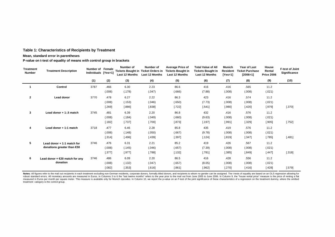
Table 1: Characteristics of Recipients by Treatment

Mean, standard error in parentheses

P-value on t-test of equality of means with control group in brackets

Treatment

NumberTreatment Description

Number of

Individuals

Female

[Yes=1]

Number of

Tickets Bought in

Last 12 Months

Number of

Ticket Orders in

Last 12 Months

Average Price of

Tickets Bought in

Last 12 Months

Total Value of All

Tickets Bought in

Last 12 Months

Munich

Resident

[Yes=1]

Year of Last

Ticket Purchase

[2006=1]

House

Rental

Price 2006

F-test of Joint

Significance

(1) (2) (3) (4) (5) (6) (7) (8) (9) (10)

1 Control 3787 .466 6.30 2.23 86.6 416 .416 .565 11.2

(.008) (.178) (.047) (.666) (7.88) (.008) (.008) (.021)

2 Lead donor 3770 .478 6.27 2.22 86.3 423 .416 .574 11.2

(.008) (.153) (.046) (.650) (7.73) (.008) (.008) (.021)

[.269] [.886] [.838] [.722] [.541] [.980] [.420] [.979] [.370]

3 Lead donor + 1:.5 match 3745 .481 6.39 2.20 86.8 432 .416 .576 11.2

(.008) (.184) (.049) (.660) (9.63) (.008) (.008) (.021)

[.182] [.737] [.700] [.873] [.197] [.991] [.329] [.905] [.752]

4 Lead donor + 1:1 match 3718 .477 6.46 2.28 85.8 435 .419 .576 11.2

(.008) (.148) (.050) (.667) (9.78) (.008) (.008) (.021)

[.314] [.496] [.439] [.397] [.124] [.819] [.347] [.785] [.481]

5 3746 .476 6.31 2.21 85.2 419 .426 .567 11.2

(.008) (.145) (.046) (.657) (7.39) (.008) (.008) (.021)

[.377] [.977] [.788] [.132] [.781] [.385] [.849] [.447] [.318]

6 3746 .486 6.09 2.20 86.5 416 .428 .556 11.2

(.008) (.132) (.047) (.657) (8.05) (.008) (.008) (.021)

[.082] [.353] [.616] [.861] [.962] [.270] [.416] [.428] [.579]

Lead donor + €20 match for any

donation

Lead donor + 1:1 match for

donations greater than €50

Notes: All figures refer to the mail out recipients in each treatment excluding non-German residents, corporate donors, formally titled donors, and recipients to whom no gender can be assigned. The t-tests of equality are based on an OLS regression allowing for robust standard errors. All monetary amounts are measured in Euros. In Columns 3 to 6 the "last twelve months" refers to the year prior to the mail out from June 2005 to June 2006. In Column 9, the "house rental price" measure is the price of renting a flat measured in Euros per month per square meter. This measure is available only for Munich zipcodes. In Column 10, we report the p-value on an F-test of the joint significance of these characteristics of a regression on the treatment dummy, where the omitted treatment category is the control group.

Table 2: Characteristics of Donors and Non Donors by Treatment

Mean, standard error in parentheses

P-value on test of equality of means between donors and non-donors in brackets, by treatment

Number of

Responses

Female

[Yes=1]

Number of Tickets

Bought in Last 12

Months

Number of Ticket

Orders in Last 12

Months

Average Price of

Tickets Bought in

Last 12 Months

Total Value of All

Tickets Bought in

Last 12 Months

Munich

Resident

[Yes=1]

Year of Last

Ticket Purchase

[2006=1]

House

Rental

Price 2006

(1) (2) (3) (4) (5) (6) (7) (8) (9)

All Donors 922 .475 8.71 2.91 87.6 642 .421 .702 11.2

(.016) (.353) (.105) (1.45) (24.9) (.016) (.015) (.021)

All Non Donors .477 6.20 2.19 86.2 414 .420 .563 11.2

(.003) (.065) (.020) (.274) (3.42) (.003) (.003) (.021)

[.896] [.000] [.000] [.341] [.000] [.965] [.000] [.657]

1 Control 142 .394 8.55 2.87 87.1 585 .380 .697 11.2

(.041) (.970) (.245) (3.65) (47.0) (.041) (.039) (.108)

[.080] [.019] [.009] [.901] [.000] [.376] [.000] [.855]

2 Lead donor 132 .530 9.52 3.36 88.1 666 .394 .742 11.3

(.044) (.954) (.374) (4.21) (66.1) (.043) (.038) (.114)

[.226] [.000] [.002] [.669] [.000] [.600] [.000] [.386]

3 Lead donor + 1:.5 match 156 .449 9.67 2.88 87.3 662 .365 .654 11.2

(.040) (1.09) (.235) (3.33) (55.1) (.039) (.038) (.113)

[.412] [.002] [.004] [.874] [.000] [.183] [.040] [.673]

4 Lead donor + 1:1 match 155 .426 7.96 2.75 88.9 619 .413 .748 11.2

(.040) (.746) (.274) (4.13) (58.2) (.040) (.035) (.108)

[.190] [.041] [.083] [.452] [.001] [.886] [.000] [.957]

5 160 .563 8.11 2.60 90.7 698 .475 .694 11.2

(.039) (.703) (.177) (3.14) (69.7) (.040) (.037) (.097)

[.025] [.010] [.028] [.079] [.000] [.206] [.000] [.887]

6 177 .486 8.58 3.07 83.8 623 .480 .684 11.2

(.038) (.719) (.243) (2.98) (63.9) (.038) (.035) (.086)

[.994] [.000] [.000] [.367] [.001] [.160] [.003] [.992]

Treatment Number and

Description

Lead donor + 1:1 match for

donations greater than €50

Lead donor + €20 match for

any donation

Notes: All figures refer to the mail out recipients in each treatment excluding non-German residents, corporate donors, formally titled donors, and recipients to whom no gender can be assigned. The tests of equality are based on an OLS regression allowing for robust standard errors. All monetary amounts are measured in Euros. In Columns 3 to 6 the "last twelve months" refers to the year prior to the mail out from June 2005 to June 2006. In Column 9, the "house rental price" measure is the price of renting a flat measured in Euros per month per square meter. This measure is available only for Munich zipcodes.

Table 3: Fundraising Outcomes by Treatment

Mean, standard error in parentheses

P-values on tests of equalities on means with comparison group in brackets

Treatment

NumberTreatment Description

Comparison

GroupResponse Rate

Total Amount

Donated

Total Amount

Raised

Average Donation

Received,

All Recipients

Average

Donation

Received

Median

Donation

Received

Average

Donation

Given

Median

Donation

Given

(1) (2) (3) (4) (5) (6) (7) (8)

1 Control .037 2.79 74.3 50 74.3 50

(.003) (.326) (6.19) (6.19)

2 Lead donor .035 4.62 132 100 132 100

(.003) (.635) (14.3) (14.3)

T1 Control [.564] [.010] [.000] [.000] [.000] [.000]

3 Lead donor + 1:.5 matching .042 4.19 151 75 101 50

(.003) (.618) (18.9) (12.6)

T1 Control [.355] [.044] [.000] [.005] [.061] [.999]

T2 Lead donor [.134] [.631] [.421] [.131] [.102] [.000]

4 Lead donor + 1:1 matching .042 3.84 185 100 92.3 50

(.003) (.526) (20.7) (10.4)

T1 Control [.352] [.086] [.000] [.000] [.136] [.999]

T2 Lead donor [.132] [.350] [.037] [.999] [.025] [.000]

5 .043 4.18 194 120 97.9 60

(.003) (.521) (19.3) (9.59)

T1 Control [.249] [.023] [.000] [.000] [.039] [.138]

T2 Lead donor [.084] [.596] [.010] [.102] [.049] [.000]

6 .047 3.27 89.2 70 69.2 50

(.003) (.353) (5.51) (5.51)

T1 Control [.036] [.314] [.073] [.024] [.539] [.999]

T2 Lead donor [.008] [.063] [.006] [.065] [.000] [.002]

Donors OnlyAll Recipients

15671 31107

1578812248

Lead donor + €20 match for any

donation

Lead donor + 1:1 matching for

donations greater than €50

14310 28620

10550 10550

17416 17416

15705 23558

Notes: All figures are based on the total sample of recipients of the mail outs excluding non-German residents, corporate donors, formally titled donors, and recipients to whom no gender can be assigned. Columns 1-4 refer to all recipients of the mail-out (donors and non-donors). Columns 5-8 refer only to donors. The test of equality of means in Columns 4, 5, and 7 are based on an OLS regression allowing for robust standard errors. The test of equality of medians in Columns 6 and 8 are based on a quantile regression. The response rate is the proportion of recipients that donate some positive amount, as reported in the donation amount column. The actual donation then received by the opera house in each treatment is reported in the donation received column. All monetary amounts are measured in Euros.

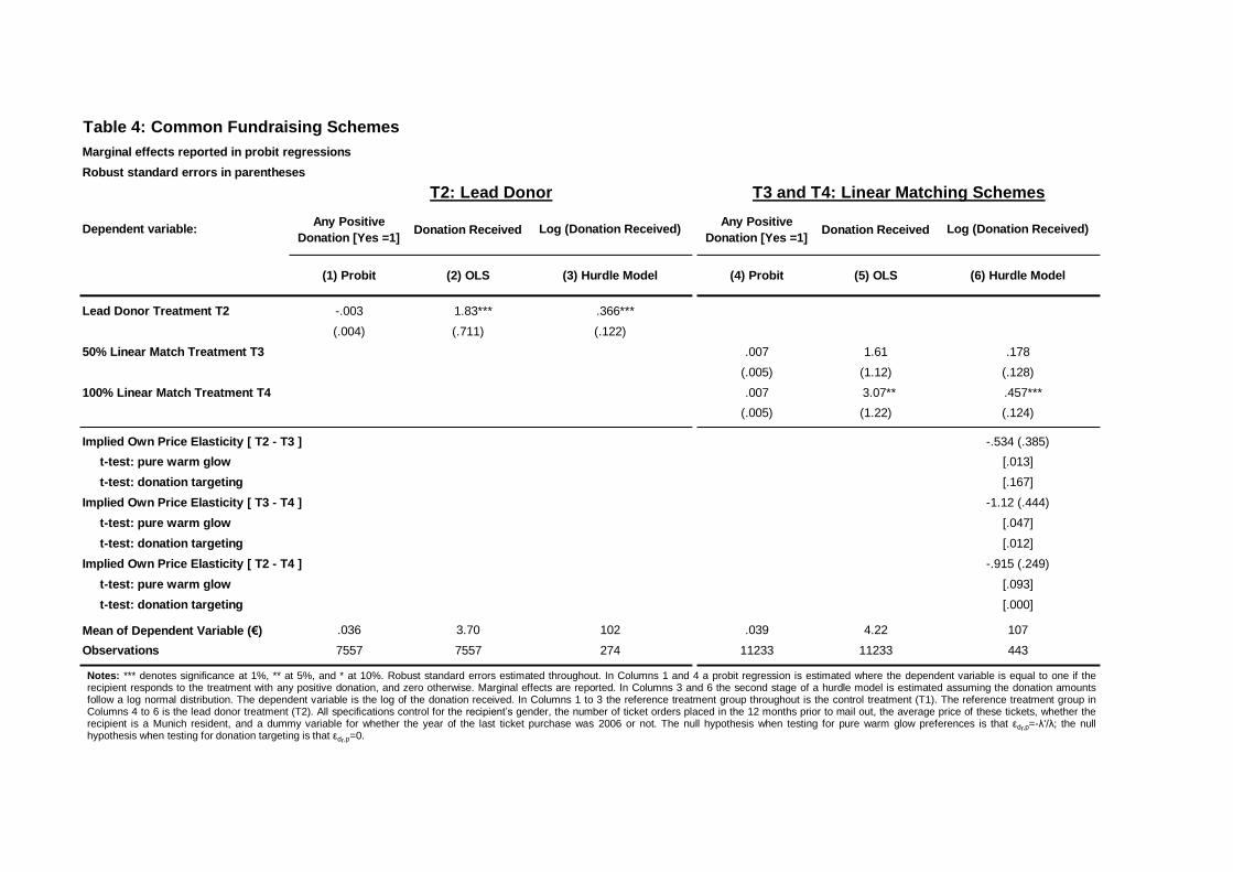
Table 4: Common Fundraising Schemes

Marginal effects reported in probit regressions

Robust standard errors in parentheses

Dependent variable:Any Positive

Donation [Yes =1]Donation Received Log (Donation Received)

Any Positive

Donation [Yes =1]Donation Received Log (Donation Received)

(1) Probit (2) OLS (3) Hurdle Model (4) Probit (5) OLS (6) Hurdle Model

Lead Donor Treatment T2 -.003 1.83*** .366***

(.004) (.711) (.122)

50% Linear Match Treatment T3 .007 1.61 .178

(.005) (1.12) (.128)

100% Linear Match Treatment T4 .007 3.07** .457***

(.005) (1.22) (.124)

Implied Own Price Elasticity [ T2 - T3 ] -.534 (.385)

t-test: pure warm glow [.013]

t-test: donation targeting [.167]

Implied Own Price Elasticity [ T3 - T4 ] -1.12 (.444)

t-test: pure warm glow [.047]

t-test: donation targeting [.012]

Implied Own Price Elasticity [ T2 - T4 ] -.915 (.249)

t-test: pure warm glow [.093]

t-test: donation targeting [.000]

Mean of Dependent Variable (€) .036 3.70 102 .039 4.22 107

Observations 7557 7557 274 11233 11233 443

T3 and T4: Linear Matching SchemesT2: Lead Donor

Notes: *** denotes significance at 1%, ** at 5%, and * at 10%. Robust standard errors estimated throughout. In Columns 1 and 4 a probit regression is estimated where the dependent variable is equal to one if the recipient responds to the treatment with any positive donation, and zero otherwise. Marginal effects are reported. In Columns 3 and 6 the second stage of a hurdle model is estimated assuming the donation amounts follow a log normal distribution. The dependent variable is the log of the donation received. In Columns 1 to 3 the reference treatment group throughout is the control treatment (T1). The reference treatment group in Columns 4 to 6 is the lead donor treatment (T2). All specifications control for the recipient’s gender, the number of ticket orders placed in the 12 months prior to mail out, the average price of these tickets, whether the recipient is a Munich resident, and a dummy variable for whether the year of the last ticket purchase was 2006 or not. The null hypothesis when testing for pure warm glow preferences is that εdr,p

=-λ'/λ; the null hypothesis when testing for donation targeting is that εdr,p

=0.

Table 5: Novel Fundraising Schemes

Marginal effects reported in probit regressions

Robust standard errors in parentheses

Dependent variable:Any Positive

Donation [Yes =1]Donation Received Log (Donation Received)

Any Positive

Donation [Yes =1]Donation Received Log (Donation Received) Log (Donation Given)

(1) Probit (2) OLS (3) Hurdle Model (4) Probit (5) OLS (6) Hurdle Model (7) Hurdle Model

100% Linear Match Treatment T4 .007 3.08** .377***

(.005) (1.22) (.105)

Non-linear Matching Treatment T5 .008* 3.85*** .560***

(.005) (1.22) (.099)

Fixed Gift Matching Treatment T6 .013*** -.372 .012 -.456***

(.004) (.750) (.112) (.104)

Mean of Dependent Variable (€) .040 6.87 173 .041 4.42 107 96

Equality of Treatments T4 and T5 [.730] [.594] [.035]

Observations 11234 11234 447 7516 7516 309 309

T5: Non-linear Matching T6: Fixed Lead Gift

Notes: *** denotes significance at 1%, ** at 5%, and * at 10%. Robust standard errors estimated throughout. In Columns 1 and 4 probit regressions are estimated where the dependent variable is equal to one if the recipient responds to the matching treatment with any positive donation, and zero otherwise. Marginal effects are reported. In Columns 3, 6 and 7 the second stage of a hurdle model is estimated assuming the donation amounts follow a log normal distribution. In Columns 3 and 6 the dependent variable is the log of the donation received. In Column 7 the dependent variable is the log of the donation given. The reference treatment group throughout is the lead donor treatment (T2). In Columns 1 to 3 we also report the p-value on the null hypothesis that the coefficients on the dummy variables for treatments T4 and T5 are equal. All specifications control for the recipient’s gender, the number of ticket orders placed in the 12 months prior to mail out, the average price of these tickets, whether the recipient is a Munich resident, and a dummy variable for whether the year of the last ticket purchase was 2006 or not.

Table 6: Model Fit from Baseline Model

Empirical and Predicted Donation Rates in Columns 1 to 3; Empirical and Predicted Conditional Average Donation Given (in Euros) in Columns 4 to 6

Standard Errors in Parentheses

(1) Empirical (2) Continuous (3) Discrete (4) Empirical (5) Continuous (6) Discrete

T1 Control .037 .037 .037 74.3 75.9 76.6

(.003) (.003) (.003) (6.19) (7.1) (7.1)

T2 Lead Donor .035 .034 .034 132 174 162

(.003) (.002) (.002) (14.3) (15.6) (11.8)

T3 Lead donor + 1:.5 match .042 .040 .040 101 119 113

(.003) (.002) (.002) (12.6) (10.8) (8.2)

T4 Lead donor + 1:1 match .042 .043 .043 92.3 90.4 87

(.003) (.003) (.003) (10.4) (8.3) (6.4)

T5 .043 .033 .034 97.9 114 107

(.003) (.002) (.002) (9.6) (9.5) (7.8)

T6 .047 .050 .044 69.2 103 112

(.003) (.007) (.004) (5.51) (21.3) (16.0)

Response Rate Average Donation Given

Lead donor + 1:1 match for

donations greater than €50

Lead donor + €20 match for

any donation

Notes: The Table shows the fit of our baseline model with a continuous choice set (Columns 2 and 5) and a discrete choice set (Columns 4 and 6) using the maximum likelihood parameter estimates from Table A1 and the sample distribution of covariates. Columns 1 to 3 report the empirical and predicted response rate (in percentage points); Columns 4 to 6 report empirical and predicted conditional average donation given (in Euros). Standard errors are in parentheses and are calculated by sampling 500 times from the distribution of parameter estimates.

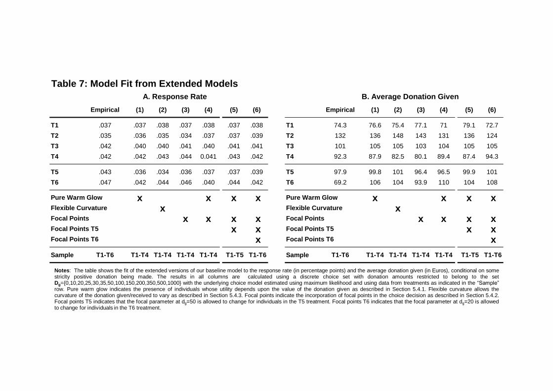
Empirical (1) (2) (3) (4) (5) (6) Empirical (1) (2) (3) (4) (5) (6)

T1 .037 .037 .038 .037 .038 .037 .038 T1 74.3 76.6 75.4 77.1 71 79.1 72.7

T2 .035 .036 .035 .034 .037 .037 .039 T2 132 136 148 143 131 136 124

T3 .042 .040 .040 .041 .040 .041 .041 T3 101 105 105 103 104 105 105

T4 .042 .042 .043 .044 0.041 .043 .042 T4 92.3 87.9 82.5 80.1 89.4 87.4 94.3

T5 .043 .036 .034 .036 .037 .037 .039 T5 97.9 99.8 101 96.4 96.5 99.9 101

T6 .047 .042 .044 .046 .040 .044 .042 T6 69.2 106 104 93.9 110 104 108

x x x x x x x x x x x x x x x x x x x x x x x x

Sample T1-T6 T1-T4 T1-T4 T1-T4 T1-T4 T1-T5 T1-T6 Sample T1-T6 T1-T4 T1-T4 T1-T4 T1-T4 T1-T5 T1-T6

Focal Points T5

Focal Points T6

Pure Warm Glow

Flexible Curvature

Focal Points

Focal Points T5

Focal Points T6

Table 7: Model Fit from Extended Models

A. Response Rate B. Average Donation Given

Pure Warm Glow

Flexible Curvature

Focal Points

Notes: The table shows the fit of the extended versions of our baseline model to the response rate (in percentage points) and the average donation given (in Euros), conditional on some striclty positive donation being made. The results in all columns are calculated using a discrete choice set with donation amounts restricted to belong to the set Dg={0,10,20,25,30,35,50,100,150,200,350,500,1000} with the underlying choice model estimated using maximum likelihood and using data from treatments as indicated in the “Sample” row. Pure warm glow indicates the presence of individuals whose utility depends upon the value of the donation given as described in Section 5.4.1. Flexible curvature allows the curvature of the donation given/received to vary as described in Section 5.4.3. Focal points indicate the incorporation of focal points in the choice decision as described in Section 5.4.2. Focal points T5 indicates that the focal parameter at dg=50 is allowed to change for individuals in the T5 treatment. Focal points T6 indicates that the focal parameter at dg=20 is allowed to change for individuals in the T6 treatment.

Table 8: Counterfactual Charitable Fundraising Schemes

T2: Lead Donor

(1) (2a) (2b) (2c) (3a) (3b) (3c) (4a) (4b) (4c) (5a) (5b) (5c) (6a) (6b) (6c)

Pre-threshold Match Rate: λ0 1 2 3 4 1 1 1 1 1 1 1 1 1 1 1 1

Post-threshold Match Rate: λ1 - - - - 1.5 2 2 1 1 1 1.5 2 2 2 2 2

Threshold: dχ - - - - 50 50 100 0 20 50 50 50 100 50 50 50

Value of Fixed Lead Gift: df - - - - - - - 20 20 20 - - - 25 75 100

Response Rate .037 .040 .041 .040 .037 .037 .037 .041 .039 .037 .037 .037 .037 .037 .037 .037

Mean Donations Given, Conditional on

a Strictly Positive Donation131 89.1 74.4 66.9 109 96.7 100 111 117 123 117 108 117 102 92.0 87.7

Average Donation Given 4.85 3.56 3.05 2.68 4.03 3.58 3.70 4.55 4.56 4.55 4.33 4.00 4.33 3.77 3.40 3.25

Linear Matching:

Higher Match Rates

Fixed Lead Gifts: Variable

Thresholds That Trigger

the Fixed Gift

Kinked Match

Functions

Non Linear Matching: Variable

Thresholds and Post-

Threshold Match Rates

Generalised

Threshold Matching

Notes: This shows outcomes for counterfactual estimates based on alternative fundraising schemes. In each column we show the predicted response rate (in percentage points), the predicted mean donation given (in Euros) conditional on a strictly positive donation being made, and the average donation given (including zeroes) (in Euros). All results are calculated using our preferred specification with a discrete choice set, pure warm glow preferences, and focal points. All donation rates and mean conditional donations are calculated using the empirical distribution of covariates observed across treatments T1 to T6. In Column 1 predicted behavior in the lead donor treatment T2 is shown. In Columns 2a to 2c we consider linear matching schemes. In Columns 3a to 3c we consider non-linear matching schemes that vary in the threshold at which the non-linearity occurs, and the post-threshold matching rate. In Columns 4a to 4c we consider variations of the fixed lead gift donation T6 where we vary the threshold at which the lead gift is provided, and the value of the lead gift. In Columns 5a to 5c we consider kinked matching functions in which two match rates are offered either side of some threshold, and in Columns 6a to 6c we consider a generalized matching scheme that encompasses the other schemes as special cases.

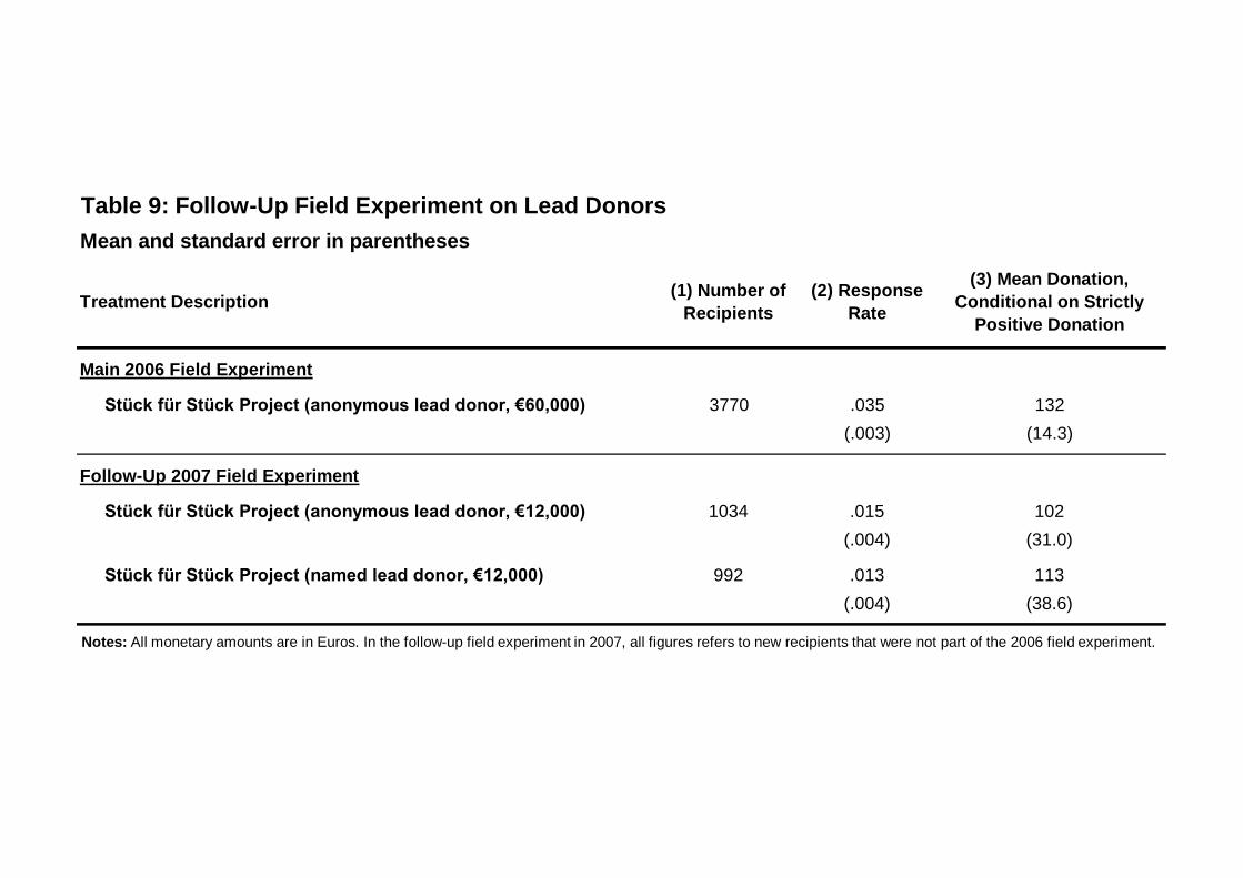
Table 9: Follow-Up Field Experiment on Lead Donors

Mean and standard error in parentheses

Treatment Description(1) Number of

Recipients

(2) Response

Rate

(3) Mean Donation,

Conditional on Strictly

Positive Donation

Main 2006 Field Experiment

Stück für Stück Project (anonymous lead donor, €60,000) 3770 .035 132

(.003) (14.3)

Follow-Up 2007 Field Experiment

Stück für Stück Project (anonymous lead donor, €12,000) 1034 .015 102

(.004) (31.0)

Stück für Stück Project (named lead donor, €12,000) 992 .013 113

(.004) (38.6)

Notes: All monetary amounts are in Euros. In the follow-up field experiment in 2007, all figures refers to new recipients that were not part of the 2006 field experiment.

Table A1: Structural Parameter Estimates

Baseline Model Using Linear Matching Treatments T1-T4

Bootstrapped Standard Errors in Parentheses

Panel A. Continuous Donations Given, dg

Constant Gender [Female =1]Munich Resident

[Yes=1]

Average Price of

Tickets Bought in

Last 12 Months

Number of Ticket

Orders in Last 12

Months

Year of Last Ticket

Purchase [2006=1]

μ0θ -3.065 -0.25 -0.157 0.268 0.051 0.484

(2.270) (0.246) (0.223) (0.324) (0.037) (0.346)

μ1θ -9.603 -0.079 -0.217 1.242 0.13 1.262

(5.154) (0.245) (0.304) (0.762) (0.073) (0.679)

σ0θ 2.008

(1.086)

σ1θ 4.656

(2.321)

α 0.011

(0.006)

Panel B. Discrete Donations Given, dg

Constant Gender [Female =1]Munich Resident

[Yes=1]

Average Price of

Tickets Bought in

Last 12 Months

Number of Ticket

Orders in Last 12

Months

Year of Last Ticket

Purchase [2006=1]

μ0θ

-2.865 -0.238 -0.149 0.263 0.049 0.464

(2.029) (0.228) (0.208) (0.304) (0.033) (0.311)

μ1θ

-8.719 -0.064 -0.205 1.117 0.12 1.16

(4.605) (0.223) (0.278) (0.700) (0.066) (0.612)

σ0θ

1.932

-0.976

σ1θ

4.313

(2.074)

α 0.011

(0.005)

Preferred ModelPanel C. Discrete Donations Given, Warm Glow and Focal Points

Constant Gender [Female =1]Munich Resident

[Yes=1]

Average Price of

Tickets Bought in

Last 12 Months

Number of Ticket

Orders in Last 12

Months

Year of Last Ticket

Purchase [2006=1]

μ0θ -6.120 -0.437 -0.267 0.506 0.091 0.851

(0.500) (0.285) (0.284) (0.373) (0.034) (0.298)

μ1θ -14.288 -0.092 -0.342 1.701 0.193 1.856

(0.681) (0.296) (0.327) (0.490) (0.035) (0.331)

σ0θ 3.546

(0.146)

σ1θ 6.962

(0.216)

α 0.022

(0.001)

πw 0.344

(0.076)

ξ20 0.031

(0.227)

ξ50 5.505

(0.655)

ξ100 13.349

(1.131)

Notes: Panels A and B show the maximum likelihood parameter estimates of our baseline model with a continuous choice set (panel A) and a discrete choice set (panel B). The choice of donation amounts under the discrete choice set specification is restricted to belong to the set Dg={0,10,20,25,30,35,50,100,150,200,350,500,1000}. Panel C shows maximum likelihood parameter estimates of our preferred specification with warm glow preferences and focal points. All estimation is performed using data from treatments T1 to T4 only, and standard errors are in parentheses. All monetary amounts are measured in 100’s of Euros. The "last twelve months" refers to the year prior to the mail out from June 2005 to June 2006. Standard errors are in parentheses and are calculated using 500 bootstrap repetitions.

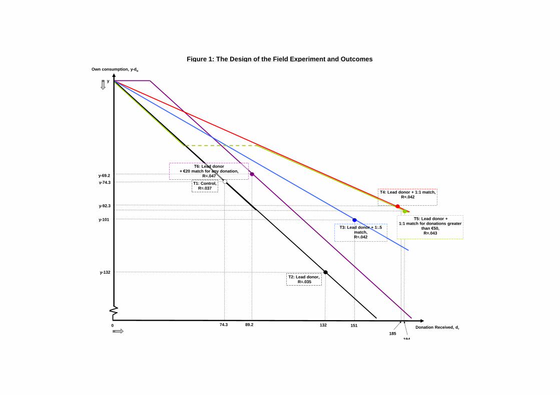
Figure 1: The Design of the Field Experiment and Outcomes

Donation Received, dr

y

y-74.3

y-132

185

0 151 74.3 132

T1: Control, R=.037

T5: Lead donor + 1:1 match for donations greater

than €50, R=.043

T6: Lead donor + €20 match for any donation,

R=.047

T3: Lead donor + 1:.5 match, R=.042

T4: Lead donor + 1:1 match, R=.042

T2: Lead donor, R=.035

y-101

y-92.3

194

y-69.2

89.2

Own consumption, y-dg

194

Figure 2: Quantile Regression Estimates of Signaling Treatment T2

-10

1

0 10 20 30 40 50 60 70 80 90 100quartileQuantile

Qu

an

tile

Reg

ressio

n E

sti

mate

OLS Estimate

Notes: Figure 2 shows the estimated quantile regression effect at each quantile of the conditional distribution of the log of donations received, and the associated 95% confidence interval. The figure also shows the coefficient on the treatment dummy variable from an OLS regression. The individual characteristics controlled for are whether the recipient is female, the number of ticket orders placed in the 12 months prior to mail out, the average price of these tickets, whether the recipient is a Munich resident, and a dummy variable for whether the year of the last ticket purchase was 2006 or not.

Figure 3: Empirical and Predicted Distributions of Donations

Notes: The figure shows the predicted and empirical distribution of positive donation amounts. Horizontal axis measure the amount of donation given, The figures are based on the preferred structural model that assumes a discrete choice set with warm glow preferences and focal points. The choice of donation amounts under the discrete choice set specification is restricted to belong to the set Dg={0,10,20,25,30,35,50,100,150,200,350,500,1000}. All estimation is performed using data from treatments T1 to T4 only.

0.000

0.005

0.010

0.015

0.020

0.025

10 20 25 30 35 50 100 150 200 350 500 1000

Treatment T1

Empirical

Predicted

0.000

0.005

0.010

0.015

0.020

0.025

10 20 25 30 35 50 100 150 200 350 500 1000

Treatment T2

Empirical

Predicted

0.000

0.005

0.010

0.015

0.020

0.025

10 20 25 30 35 50 100 150 200 350 500 1000

Treatment T3

Empirical

Predicted

0.000

0.005

0.010

0.015

0.020

0.025

10 20 25 30 35 50 100 150 200 350 500 1000

Treatment T4

Empirical

Predicted

0.000

0.005

0.010

0.015

0.020

0.025

10 20 25 30 35 50 100 150 200 350 500 1000

Treatment T5

Empirical

Predicted

0.000

0.005

0.010

0.015

0.020

0.025

10 20 25 30 35 50 100 150 200 350 500 1000

Treatment T6

Empirical

Predicted

Figure A1: Giving Behavior in the

Non-Linear Matching Treatment T5

Notes: The yellow area corresponds to the set of parameters where dg>50. The orange area is the parameter set where dg=50. The brown area is the parameter set where 0<dg<50.

50gd

50gd

500 gd

Appendix: The Mail Out Letter (Translated)

Bayerische Staatsoper Staatsintendant Max-Joseph-Platz 2, D-80539 München www.staatsoper.de [ADDRESS OF RECIPIENT] Dear [RECIPIENT], The Bavarian State Opera House has been investing in the musical education of children and youths for several years now as the operatic the art form is in increasing danger of disappearing from the cultural memory of future generations. Enthusiasm for music and opera is awakened in many different ways in our children and youth programme, “Erlebnis Oper” [Experience Opera]. In the forthcoming season 2006/7 we will enlarge the scope of this programme through a new project “Stück für Stück” that specifically invites children from schools in socially disadvantaged areas to a playful introduction into the world of opera. Since we have extremely limited own funds for this project, the school children will only be able to experience the value of opera with the help of private donations. [This paragraph describes each matching scheme and is experimentally varied as described in the main text of the paper]. As a thank you we will give away a pair of opera tickets for Engelbert Humperdinck’s “Konigskinder” on Wednesday, 12 July 2006 in the music director’s box as well as fifty CDs signed by Maestro Zubin Mehta among all donors. You can find all further information in the enclosed material. In case of any questions please give our Development team a ring on [phone number]. I would be very pleased if we could enable the project “Stück für Stück” through this appeal and, thus, make sure that the operatic experience is preserved for younger generations. With many thanks for your support and best wishes, Sir Peter Jonas, Staatsintendant

Appendix: The Mail Out Letter (Translated)

“Stück für Stück” The project “Stück für Stück” has been developed specifically for school children from socially disadvantaged areas. Musical education serves many different functions in particular for children and youths with difficult backgrounds -- it strengthens social competence and own personality, improves children’s willingness to perform, and reduces social inequality. Since music education plays a lesser and lesser role in home and school education, the Bavarian State Opera has taken it on to contribute to it ourselves. The world of opera as a place of fascination is made attainable and accessible for young people. In drama and music workshops, “Stück für Stück” will give insights into the world of opera for groups of around 30 children. They will be intensively and creatively prepared for a subsequent visit of an opera performance. These workshops encourage sensual perception – through ear and eye but also through scenic and physical play and intellectual comprehension – all of these are important elements for the workshops. How does Orpheus in “Orphee and Eurydice” manage to persuade the gods to let him save his wife from the realm of dead? Why does he fail? Why poses the opera “Cosi fan tutte” that girls can never be faithful? It is questions like these that are investigated on the workshops. The workshops are also made special through the large number and variety of people who are involved in them: musicians, singers, directors, and people from many other departments, ranging from costumes and makeup to marketing. The participants in each workshop work through an opera’s storyline, and are introduced to the production and will meet singers in their costumes as well as musicians. This makes the workshops authentic. After the workshops the participants are invited to see the actual opera production. Through your donation the project “Stück für Stück” will be made financially viable so that we can charge only a small symbolic fee to the participants. This makes it possible to offer our children and youth programme also to children from socially disadvantaged backgrounds that can, thus, learn about the fascination of opera. Note: In German, Stück für Stück is a wordplay --- “Stück” meaning “play” as in drama and “Stück für Stück” being an expression for doing something bit by bit.