Mathematical & Computational Applications, Vol. 1, No.1, pp 165-171, 1996© Association for Scientific Research

COMPARING ARTIFICIAL NEURAL NETWORKS (ANN) IMAGECOMPRESSION TECHNIQUE WITH DIFFERENT IMAGE COMPRESSION

TECHNIQUES

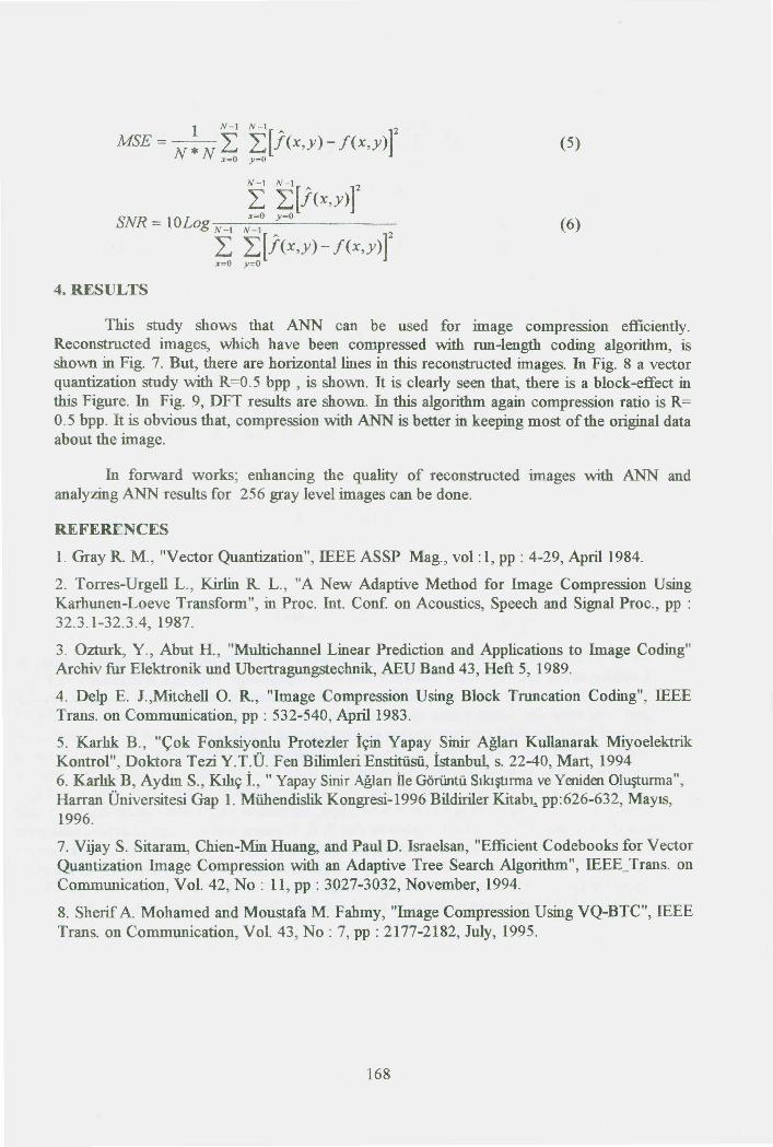
Bekir KARLIK*, Serkan AYDIN*, llker KIlJ<;** Celal Bayar U.,Electric-Eleetronic Eng. Dep., Manisa

Abstract: In this paper it is presented that, 256x256 16 gray level images can be compressedfast and efficiently by using neural networks . Compression results were compared with theother methods according to mean square error (MSE) and visual of the image and it is seen thatby further works on ANN the images can be compressed better.

An 640x480 , 256 gray level image needs about 310 Kbytes memory. According to thestandard of Europe CCIR or USA-RS 170 monochrome, an image is renewed 25 times in asecond. 64Ox480, 30 video images are stored into the video RAM in a second by using ascorpion card. This means in real time we have to transfer 9 Mbytes data into the computermemory in a second. It is quite difficult almost impossible. But if we achieve this work we need3.2 GBytes memory for an hour video signal. So it is not practical. We have different imagecompression algorithms as JPEG and MPEG that the compressed image data needs lessmemory and the compression work doesn't take much time.

Image compression and reconstruction are important problems. An other problem isdecreasing of the compression and reconstruction time duration. Especially, in real time,decreasing the computation time is an important advantage.

The purpose of image compression is decreasing the memory where the compressedimage is stored in. The reconstructed image data quality must be reasonable.

There are quite a lot of methods about image compression. These methods are dividedin two classes ; lossless and lossy. In lossless algorithm like Huffinan coding the compressionratio is limited and very low. In lossy compression algorithms we can obtain high compressionrates but by the way the MSE also increases.

Run-length coding, vector quantization [1] [7],transform coding [2],predictive coding[3] and block truncation coding [8] are some of the lossy compression techniques.

In run-length algorithm first pixel value is assumed as the reference .If the followingpixel values do not exceed a threshold, then run counter is increased one for each pL'(el.Otherwise "1" is loaded into the run counter and the following first pixel becomes the newreference value. Because there are likely to be runs of length» 1 in the compressed imagerepresentation, the resulting compressed data set will be smaller than the raw image data. Theseeffects are highly dependent on the threshold T, which mu!>tbe chosen to yield both areasonable image representation(i.e., the reconstructed image should appear subjectively

"close" to the uncompressed image and a reasonable number of nms, each consisting of areasonable number of pixels.

In Run-length method if the compression ratio is increased, horizontal lines are seen onthe image causing noise.

In Vector Quantization the image is formed with two dimensional blocks. Each block isrepresented by a vector. All vectors of this algorithm are selected from a codebook table whichis formed before the compression. The problems of this algorithm are block effect and edgedistortion.

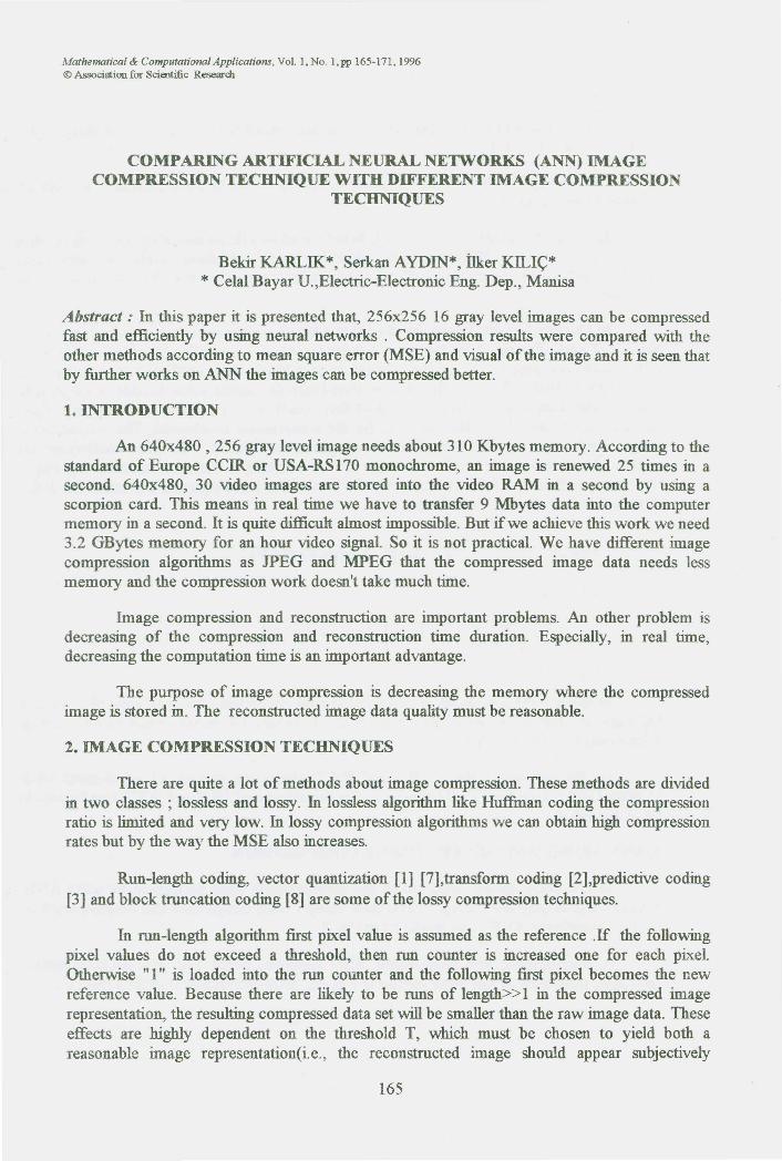
In Discrete Fourier Transform algorithm again the image is formed by two dimensionalblocks. Discrete Fourier Transform of each block consist of coefficients. Number of thesecoefficients is as same as the number of pixels in each block. Each coefficient is consist of realand imaginary parts. These coefficients are stored into the memory one by one in the zig-zagorder. In the compression algorithm some of these coefficients are ignored and the rest of thecoefficients are stored into the memory. So the compression is achieved. The reconstructedimage quality is dependent on the amount of ignored coefficient. The more coefficients areused in the compression the better image can be obtained in the reconstruction algorithm.Equation 1 presents the DFT (Discrete Fourier Transform) and equation 2 presents the IDFT(Inverse Discrete Fourier Transform)

1 N-l N-l

F(u, v) = - L Lf(x,y)exp[- j2n(ux + ty) / N]N x=O y=O

u,v = 0,1,2, N -1

1 N-l N-lf(x,y) = -L LF(u,v)exp[j2n{ux +ty) / N]

N u=O v=o

x,y = 0,1,2, N -1

In figure 2 the zig-zag order is shown. The fist coefficient of the rig-zag order is calledDC value the rest of the coefficients are called AC values. DC value consist of more imageinformation than the AC values do.

As the equations exhibit, DFT and IDFT need quite amount of calculations whileDiscrete Cosine Transform (DCT) doesn't. The formulation ofDCT and IDCT can be seen inEq. 3 and Eq. 4.

3. ANN APPROACH FOR THE IMAGE COMPRESSION

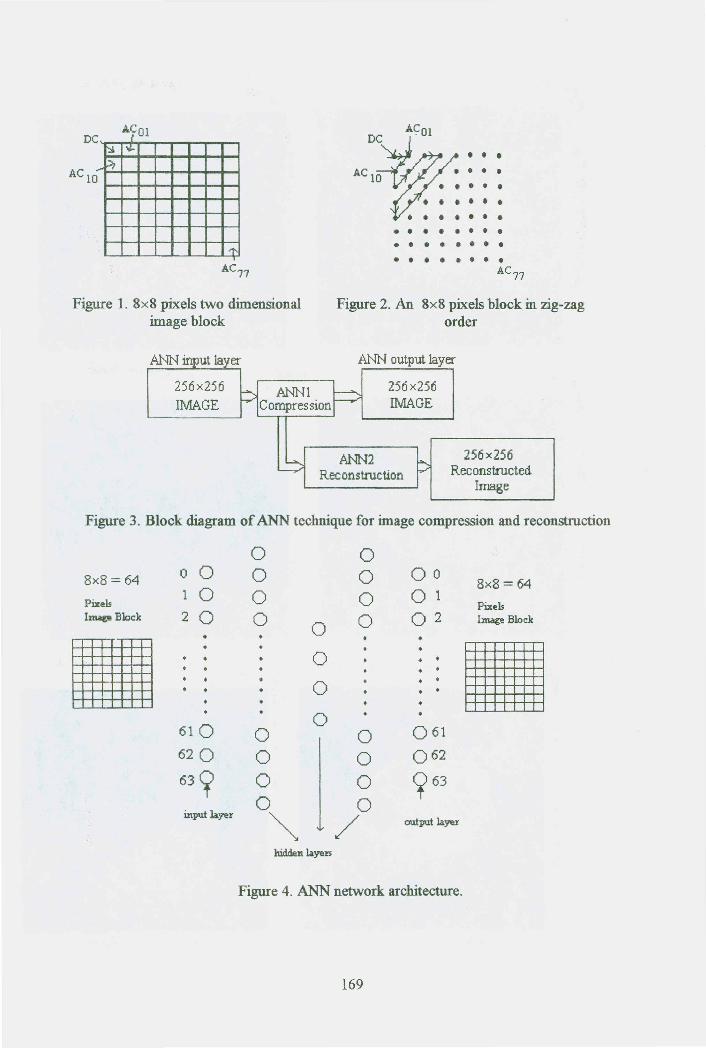
In this study, image compression and reconstruction were performed by using ANN.256x256 digital gray-level images were used. Images were compressed and reconstructed byusing two different ANN stage, as shown in Fig. 3.

A multi-layered and feedforward ANN network, which has error-backpropagationalgorithm, were used in this paper (shown in Fig. 4). ANN architecture is in the form of

N-l N-.l ~(2X + l)U) ~(2 + 1) )C(u, v) = a(u)a(v) L L!(x,y)co 1T co y VlTx=O y=o 2N 2N

11

..{ija(u)= H;

!(X,y) = ~ 21a(u)a(v)C(u, v)COf (2x + 1)UlT) cof (2y + 1)VlT)

u=o v=o '- 2N '- 2N1

..{ija(u) = H;

64:70:4:70:64. Compressed data were obtained from the hidden layer, which has four neurons.Learning speed and rate were taken 0.9 and 0.7, respectively. Network architecture in Fig. 4was used for teaching. After the teaching phase, the architecture was split into two part; the firstpart was used for compression and the other part was used for reconstruction. In Fig. 5original (left) the axial cranium section passing through sifenoidal sinus (in bone algorithm, inpontin sifenoid and in two temporal, there is subarachnoidal air collections) and (right) the axialcranium section passing through the venticular plate (the algorithm in soft tissues, mass isobserved in gray matter, white matter and intraventicular) images are shown. Images,compressed by using ANN at a rate ofR=0.5 bpp, are seen in Fig. 6. Run-length coding, vectorquantization and DFT results are given in Fig. 7, 8, 9, respectively,. Compression results fromANN were taken in real-time. If a codebook, which is formed by 16 elements, is used then theMSE and SNR values are 9.792, and 0.589302 for the image on the left handside of the page,respectively. For the image on the right handside of the page, these values are 8.859 and1.04087. MSE formulation is shown in Eq. 5 and SNR formulation is given by Eq. 6.

1 N~ N~ 2

MSE = * z: Z:[J(X,y)- !(X,y)]N N x=o y=o

N-l N-lz: Z:[J(X,y)fSNR = lOLou __ x_=O_y=_O _

o N-l N-l

L Z:[](X,y) - !(X,y)fx=O y=O

This study shows that ANN can be used for image compression efficiently.Reconstructed images, which have been compressed with run-length coding algorithm, isshown in Fig. 7. But, there are horizontal lines in this reconstructed images. In Fig. 8 a vectorquantization study with R=0.5 bpp , is shown. It is clearly seen that, there is a block-effect inthis Figure. In Fig. 9, DFT results are shown. In this algorithm again compression ratio is R=0.5 bpp. It is obvious that, compression with ANN is better in keeping most of the original dataabout the image.

In forward works; enhancing the quality of reconstructed images with ANN andanalyzing ANN results for 256 gray level images can be done.

REFERI:NCES1. Gray R. M., "Vector Quantization", IEEE ASSP Mag., vol :1, pp : 4-29, April 1984.

2. Torres-Urgell L., Kirlin R. L., "A New Adaptive Method for Image Compression UsingKarhunen-Loeve Transform", in Proc. Int. Conf. on Acoustics, Speech and Signal Proc., pp :32.3.1-32.3.4, 1987.

3. Ozturk, Y., Abut H., "Multichannel Linear Prediction and Applications to Image Coding"Arehiv fur Elektronik und Ubertragungsteehnik, AEU Band 43, Heft 5, 1989.

4. Delp E. l,Mitchell O. R., "Image Compression Using Block Truncation Coding", IEEETrans. on Communication, pp : 532-540, April 1983.

5. Karhk B., "C;ok Fonksiyonlu Protezler i9in Yapay Sinir Aglan Kullanarak MiyoelektrikKontrol", Doktora Tezi Y.T.U. Fen Bilimleri Enstitiisii, istanbul, s. 22-40, Mart, 19946. Karhk B, AydIn S., Kl119i., " Yapay SinirAglan he GortintiiSlk1~rma ve YenidenOlU$urma",Harran Universitesi Gap 1. MUhendislikKongresi-1996 Bildiriler Kitabl,.pp:626-632, MaylS,1996.

7. Vijay S. Sitaram, Chien-Min Huang, and Paul D. Israelsan, "Efficient Codebooks for VectorQuantization Image Compression with an Adaptive Tree Search Algorithm", IEEE_Trans. onCommunication, Vol. 42, No : 11, pp : 3027-3032, November, 1994.

8. Sherif A. Mohamed and Moustafa M. Fahmy, "Image Compression Using VQ-BTC", IEEETrans. on Communication, Vol. 43, No: 7, pp : 2177-2182, July, 1995.

I~ I~~

'!'

••••••••••••••••••••••••

ACn

Figure 1. 8x8 pixels two dimensionalimage block

Figure 2. An 8x8 pixels block in zig-zagorder

256x256IMAGE

ANN 1Compression

ANN output layer

256 x256IMAGE

ANN2Reconstruction

256x256Reconstructed

Image

Figure 3. Block diagram of ANN technique for image compression and reconstruction

0 08x8 = 64 0 0 0 0 00

8x8 = 64Pixels

1 0 0 0 01Pixels

Image Block 2 0 0 0 02 Image Block0

•0 • •

•0

610 0 0610 0620 0 0 06263 » 0 0 » 63

0 0mputhyu

~ / output layer

hidden layers

Figure 4. ANN network architecture.