comparative study of the martian suprathermal electron...

This article has been accepted for publication and undergone full peer review but has not been through the copyediting, typesetting, pagination and proofreading process which may lead to differences between this version and the Version of Record. Please cite this article as doi: 10.1002/2016JA023205

© 2016 American Geophysical Union. All rights reserved.

Comparative study of the Martian suprathermal electron depletions based on Mars

Global Surveyor, Mars Express and Mars Atmosphere and Volatile Evolution missions

observations

M. Steckiewicz (1,2), P. Garnier (1,2), N. André (1,2), D. L. Mitchell (3), L. Andersson (4),

E. Penou (1,2), A. Beth (5), A. Fedorov (1,2), J.-A. Sauvaud (1,2), C. Mazelle (1,2), D. A.

Brain (4), J.R. Espley (6), J. McFadden (3), J. S. Halekas (7), D. E. Larson (3), R. J. Lillis (3),

J. G. Luhmann (3), Y. Soobiah (6), and B.M. Jakosky (4)

(1) Université de Toulouse; UPS-OMP; IRAP; Toulouse, France (2) CNRS; IRAP; 9 av.

Colonel Roche, BP 44346, F-31028 Toulouse cedex 4, France (3) Space Sciences Laboratory,

University of California, Berkeley, California, USA (4) Laboratory for Atmospheric and

Space Physics, University of Colorado Boulder, Boulder, Colorado, USA (5) Department of

Physics, Imperial College London, Prince Consort Road, London SW7 2AZ, United

Kingdom (6) NASA Goddard Space Flight Center, Greenbelt, Maryland, USA (7)

Department of Physics and Astronomy, University of Iowa, Iowa City, Iowa, USA

Corresponding author: Morgane Steckiewicz, IRAP, 9 avenue du colonel Roche, BP 44346 –

31028 Toulouse Cedex 4, France ([email protected])


Key points:

Automatic detection of suprathermal electron depletions observed by three spacecraft

(MGS, MEX and MAVEN) during seventeen years

At high altitudes electron depletions are clearly observed by the 3 spacecraft over

crustal magnetic field sources

At low altitudes interaction with crustal magnetic fields is no longer the dominant

creation process for electron depletions


Abstract

Nightside suprathermal electron depletions have been observed at Mars by three

spacecraft to date: Mars Global Surveyor (MGS), Mars EXpress (MEX) and the Mars

Atmosphere and Volatile EvolutioN (MAVEN) mission. This spatial and temporal diversity

of measurements allows us to propose here a comprehensive view of the Martian electron

depletions through the first multi-spacecraft study of the phenomenon. We have analyzed

data recorded by the three spacecraft from 1999 to 2015 in order to better understand the

distribution of the electron depletions and their creation mechanisms. Three simple criteria

adapted to each mission have been implemented to identify more than 134 500 electron

depletions observed between 125 and 900 km altitude. The geographical distribution maps of

the electron depletions detected by the three spacecraft confirm the strong link existing

between electron depletions and crustal magnetic field at altitudes greater than 170 km. At

these altitudes, the distribution of electron depletions is strongly different in the two

hemispheres, with a far greater chance to observe an electron depletion in the Southern

hemisphere, where the strongest crustal magnetic sources are located. However, the unique

MAVEN observations reveal that below a transition region near 160-170 km altitude the

distribution of electron depletions is the same in both hemispheres, with no particular

dependence on crustal magnetic fields. This result supports the suggestion made by previous

studies that these low altitudes events are produced through electron absorption by

atmospheric .

Index terms: Mars (6225), Planetary Magnetosphere (2756), Planetary Ionospheres (2459),

Atmospheres (5405), Ionosphere/atmosphere interactions (2427)

Key words: Mars, MAVEN mission, MGS mission, MEX mission, nightside suprathermal

electron depletions


1. Introduction

At the present time, Mars does not possess any global dynamo magnetic field.

However, localized magnetic fields of crustal origin provide evidence of an ancient dynamo

which existed prior to 4 billion years ago [Lillis et al., 2008, 2013]. These crustal fields can

reach intensities exceeding 200 nT at 400 km in the Southern hemisphere [Acuña et al.,

2001]. Hence Mars does not possess a global intrinsic magnetosphere, but rather several

mini-magnetospheres induced by closed-loops of crustal magnetic field (where magnetic field

lines are connected at both ends to the crust). These structures can extend to hundreds of

kilometers above the surface with sufficient magnetic pressure to stand off the solar wind

flow up to 1000 km [Brain et al., 2003]. The inner magnetic field lines are then isolated from

the Interplanetary Magnetic Field (IMF). The magnetic topology near Mars is thus quite

complex with closed-loops of crustal magnetic field, open field lines connecting the crust to

the IMF, and draped field lines unconnected to the crust [Nagy et al., 2003; Bertucci et al.,

2003; Brain et al., 2007].

Mars is surrounded by a thin dominated atmosphere. The solar extreme ultra-

violet radiations impinging the neutral part of this atmosphere lead to the creation of the

dayside Martian ionosphere. However, the photoelectrons liberated in the dayside of Mars

mainly from ionization of atmospheric and by solar photons are also observed in the

nightside hemisphere [Frahm et al., 2006]. The nightside Martian ionosphere is maintained

by transport processes from the dayside (e.g. horizontal transport of photoelectrons from day-

to-nightside along draped magnetic field lines [Ulusen and Linscott, 2008; Fränz et al.,

2010]), as well as by production processes such as electron impact ionization of precipitating

magnetosheath electrons [Fillingim et al., 2010; Lillis et al., 2011; Lillis and Brain, 2013].


The nightside ionosphere still remains an unfamiliar and mysterious place. Several

studies have shown that the nightside ionosphere is irregular, spotty, faint and complex

[Zhang et al., 1990; Nemec et al., 2010; Duru et al., 2011; Withers et al., 2012]. Using Mars

Global Surveyor (MGS) Electron Reflectometer (ER) measurements, Mitchell et al. [2001]

first observed that the nightside ionosphere was punctuated by abrupt drops of the

instrumental count rate by up to three orders of magnitude to near background levels across

all energies, hence calling them “plasma voids”. These structures seemed to be observed

where closed crustal magnetic loops existed at 400 km on the nightside, i.e. they did not

connect with the magnetotail and hence tail electrons could not access them. On the dayside,

these loops can trap ionospheric plasma, including suprathermal photoelectrons. When they

travel to the nightside, the electrons are removed through a combination of outward diffusion,

scattering, and interactions with the collisional thick atmosphere at lower altitudes.

Meanwhile, the external sources of plasma (solar wind plasma traveling up the magnetotail

and ionospheric plasma) are excluded from the inner layers of the closed field regions, so that

sinks overpass sources thus creating plasma voids. The topology of the crustal magnetic

fields can therefore significantly influence the structure of the nightside ionosphere.

Based on 144 passages of Mars EXpress (MEX) at low altitudes, Soobiah et al. [2006]

observed thanks to the Analyser of Space Plasmas and Energetic Atoms (ASPERA-3) that the

electrons flux underwent significant changes close to crustal magnetic fields. Intensified flux

signatures were observed mainly on the dayside whereas flux depletions were features of the

nightside hemisphere. Through a study over seven and a half years of the MGS mission,

Brain et al. [2007] showed statistically that plasma voids are indeed concentrated near strong

crustal magnetic fields and that very few voids are seen at large distances from crustal

magnetic sources. This study also revealed that plasma voids are surrounded by areas with

trapped and conic electron pitch angle (angle between the electron velocity and the magnetic


field vectors) distributions (PADs), consistent with the idea of closed magnetic field lines and

indicating that the outer layers of closed magnetic field regions are populated thanks to

source processes such as reconnection with the draped IMF.

Furthermore, the long-term statistical survey by Brain et al. [2007] highlighted that

hardly any plasma voids are observed on the dayside (defined as Solar Zenith Angle (SZA)

greater than 90°). This means that when the crustal magnetic loops rotate to the dayside, they

trap newly created ionospheric plasma. As the ionospheric plasma is homogeneously created

in the dayside, voids are essentially never seen on this side of Mars. While plasma voids are

restricted to the nightside, studies made with MEX data by Soobiah et al. [2006] and Duru et

al. [2011] showed no dissymmetry between the dawn and the dusk side. Plasma voids are

globally distributed regardless of nightside local time (18h00-24h00; 00h00-06h00), within

the limits of their studies.

Crustal magnetic loops do not necessarily stay closed as the planet rotates [Ma et al.,

2014] and crustal fields can connect and reconnect with the piled-up, draped and dynamic

IMF. Hence, when they travel to the nightside, regions with strong enough horizontal crustal

fields are able to stand off the IMF effects. The crustal magnetic loops in these regions thus

stay closed all the way across the nightside and are populated by permanent plasma voids,

which means we can observe this phenomena during each passage above such regions on the

nightside. On the other hand, regions with weaker horizontal fields are essentially

intermittently populated with plasma voids, depending on the external drivers. For low and

moderate solar wind pressure crustal magnetic loops are closed and devoid of plasma.

However, for high solar wind pressure the crustal field lines open up and get connected to the

IMF. These weak crustal magnetic field regions are then filled with solar wind plasma

travelling through the tail [Lillis and Brain, 2013].


More recently, Hall et al., [2016] used the rapid reductions of a proxy measurement of

the electron flux derived from the MEX ASPERA-3 ELectron Spectrometer (ELS) electron

flux measurements integrated across the 20-200 eV energy range to automatically identify

plasma voids. The study covers approximately ten years of the MEX mission from 2004 to

2014 and is restricted to the illuminated induced magnetosphere (region of space inside the

magnetic pileup boundary and outside the cylindrical shadow of the planet). Using this

method, plasma voids were detected amongst 56% of the orbits under study, from 266 km

(MEX lowest periapsis) to 10 117 km. Statistical study of the distribution of these events

showed that approximately 80% of them occurred below 1 300 km, predominantly at SZA

between 90° and 120°. Study of the spatial and altitudinal distributions of the detected plasma

voids confirmed the strong link existing between the plasma voids occurrence and the

magnitude of the crustal magnetic field. The bigger the source was, the higher plasma voids

could be observed. However, some regions appears to be in contradiction with this global

behavior which suggests that other processes are involved in plasma void creation such as the

interaction between the solar wind and the Martian plasma.

All these results have been obtained from MGS and MEX data that have several

constraints. MGS did not carry any ion spectrometer and was fixed in local time at 2 a.m./ 2

p.m. via a circular orbit (altitude between 370 to 430 km). MEX on the other hand does not

carry any magnetometer and has a periapsis between 245 and 365 km. The MAVEN

spacecraft entered into orbit around Mars in September 2014 with a complete suite of plasma

and field instruments, including a magnetometer, two ion and one electron spectrometers.

The altitude of the spacecraft reaches 150 km during nominal orbits and is periodically

lowered down to 125 km for five-day periods known as “deep dips” [Bougher et al., 2015],

which allows measurements of these plasma phenomena at previously unsampled altitudes.

Initial results on the plasma voids observed by MAVEN above the Northern hemisphere was


then investigated by Steckiewicz et al. [2015]. At the time of that initial study, the data

available were restricted to latitudes between 20° and 74° North. This multi-instrument study

leads to rename the “electron plasma voids” into “nightside suprathermal electron depletions”

(hereinafter referred as electron depletions). It suggested that the distribution of electron

depletions is highly dependent on altitude. Above a transition region near 160-170 km

altitude, electron depletions are strongly linked to horizontal crustal magnetic fields as

previously shown by MEX and MGS observations. However, below that transition region the

distribution was found to be more homogeneous, irrespective of crustal magnetic field

sources. Thus, two main electron sinks leading to the creation of electron depletions have

been identified: the exclusion by closed crustal magnetic loops and the absorption by

atmospheric . These two processes seem to always play a role in electron depletions

creation but have two different predominance areas: the exclusion by closed crustal magnetic

sources is predominant at high altitudes whereas absorption by atmospheric is

predominant at low altitudes.

The present paper takes advantage of the different characteristics of these three

missions to study the geographical and altitudinal distributions of electron depletions from

different points of view. MGS data are used from 1999 to 2006 in order to take extensively

advantage of the mapping circular orbit at a roughly constant altitude ( of the

spacecraft, allowing observations of the phenomenon every two hours over the whole range

of possible latitudes [-90°; 90°]. MEX data are used from 2004 to 2014, which gives us an

unparalleled long-term view of the phenomenon at both relatively low (down to 300 km)

and high altitudes. Finally, MAVEN data are used from October 2014 to November 2015.

During this time period the spacecraft covered both hemispheres except the poles but due to

this short duration and MAVEN orbital parameters, all latitudes are not yet covered at all

possible altitudes. Even though the coverage and duration of this dataset is much lower than


those of MGS and MEX, MAVEN reached during this time period altitudes down to 125 km

which are unsampled by MGS nor MEX.

This huge data set gathering observations made over 17 years by different instruments

reaching different altitude regimes enables us to compare events observed in similar

conditions (several spacecraft in the same region) and enrich this joint vision with new

observations closer to the surface (with MAVEN). We first show examples of how electron

depletions are observed by MGS, MEX, and MAVEN, then describe the three criteria used to

automatically detect electron depletions in each mission electron spectrometer measurements.

An exhaustive dataset of electron depletions derived from these three criteria is then used to

compare their geographical distribution with the location of crustal magnetic sources. We

finally investigate and compare the altitude distributions obtained with MAVEN and MEX,

before a conclusion ends the paper.


2. Three spacecraft, three different perspectives of suprathermal

electron depletions

Martian suprathermal electron depletions have been observed to date by three

spacecraft: MGS, MEX, and MAVEN. The last two are still in good operating condition at

the time of writing. Figures 1, 2 and 3 display plasma observations of these structures made

chronologically by MGS, MEX, and MAVEN respectively and are described next in more

details. The improved performances of the plasma instrument suite over the different

missions allow now for a more accurate understanding of electron depletions.

All the ephemerides used in this paper are expressed in the MSO (Mars-centric Solar

Orbital) coordinates defined as follows: the origin is the center of Mars, the X axis points

from the center of Mars to the Sun, Y points opposite to Mars‟ orbital angular velocity and Z

completes the right-handed set so that the frame rotates slowly as Mars orbits the Sun. The

nightside is here considered as X<0. However, the real border between sunlit and dark sides

occurs at different SZA for different altitudes. Hence if an electron depletion is observed in

the nightside, it can be to some extent in the illuminated terminator region.

2.1. MGS: first observations

The Mars Global Surveyor spacecraft was placed in its mapping orbit around Mars on

March 9, 1999 [Albee et al., 2001]. This orbit was nearly circular, sun-synchronous, near-

polar, and at an altitude varying between 368 and 438 km which corresponded to a period of

approximately 2 hours. The orbit was also fixed at a local time of 2 a.m. /2 p.m. Contact with

the spacecraft was lost in early November 2006. The MGS magnetic field experiment was

composed of two redundant triaxial fluxgate magnetometers (MAG) and an electron


reflectometer (ER) [Acuña et al., 2001]. MAG was able to detect ambient magnetic fields

from to and ER measured electrons in 19 logarithmically spaced energy

channels ranging from 10 eV to 20 keV with an energy resolution of

(full width at

half maximum). MGS did not carry an ion spectrometer.

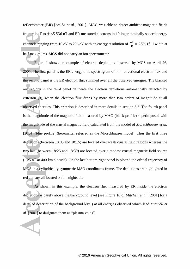
Figure 1 shows an example of electron depletions observed by MGS on April 26,

2005. The first panel is the ER energy-time spectrogram of omnidirectional electron flux and

the second panel is the ER electron flux summed over all the observed energies. The blacked

out regions in the third panel delineate the electron depletions automatically detected by

criterion (3), when the electron flux drops by more than two orders of magnitude at all

observed energies. This criterion is described in more details in section 3.3. The fourth panel

is the magnitude of the magnetic field measured by MAG (black profile) superimposed with

the magnitude of the crustal magnetic field calculated from the model of Morschhauser et al.

[2014] (blue profile) (hereinafter referred as the Morschhauser model). Thus the first three

depletions (between 18:05 and 18:15) are located over weak crustal field regions whereas the

two last (between 18:25 and 18:30) are located over a modest crustal magnetic field source

( 25 nT at 400 km altitude). On the last bottom right panel is plotted the orbital trajectory of

MGS in a cylindrically symmetric MSO coordinates frame. The depletions are highlighted in

red and are all located on the nightside.

As shown in this example, the electron flux measured by ER inside the electron

depletions is barely above the background level (see Figure 10 of Mitchell et al. [2001] for a

detailed description of the background level) at all energies observed which lead Mitchell et

al. [2001] to designate them as “plasma voids”.


2.2. Mars EXpress

The Mars Express spacecraft was inserted into orbit around Mars in January 2004. Its

orbit is highly elliptical, with a periapsis altitude between 245 and 365 km and an apoapsis

altitude of 10 000 km which implies a period of 6.75h. The inclination of the orbit is 86°

and it precesses slowly [Chicarro et al., 2004]. The ASPERA-3 experiment is composed of

four instruments including the Electron Spectrometer (ELS) and the Ion Mass Analyzer

(IMA) [Barabash et al., 2004]. The IMA sensor measures 3D-fluxes of different ion species

with a mass-to-charge ratio (m/q) resolution of 1, 2, 4, 8, 16 and >20 in the energy range

0.01-30 keV/q, with an energy resolution of

. The ELS instrument measures the

electron fluxes in the energy range 0.001 – 20 keV/q in 128 logarithmically-spaced energy

channels with an energy resolution of

(which is the best energy resolution among

the electron spectrometers of the three spacecraft, see Table 1). In general, ELS has been

operated in four different modes (Default/Survey mode, Linear mode, 1s mode and 32 Hz

mode), differing mainly in the energy ranges, the energy steps and the measuring cadences

used (see Frahm et al., [2006] and Hall et al., [2016] for more details about the different ELS

modes). In this study, we only include measurements when ELS is operating in Survey mode.

Mars Express does not carry a magnetometer.

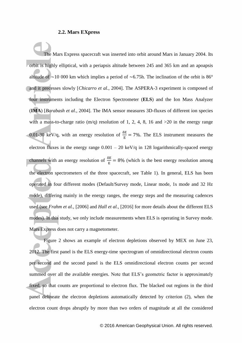
Figure 2 shows an example of electron depletions observed by MEX on June 23,

2012. The first panel is the ELS energy-time spectrogram of omnidirectional electron counts

per second and the second panel is the ELS omnidirectional electron counts per second

summed over all the available energies. Note that ELS‟s geometric factor is approximately

fixed, so that counts are proportional to electron flux. The blacked out regions in the third

panel delineate the electron depletions automatically detected by criterion (2), when the

electron count drops abruptly by more than two orders of magnitude at all the considered


energies and thus reaches the background noise level ( 40 c/s . This criterion is described in

more details in section 3.2. The fourth panel is the energy-time spectrogram of the

omnidirectional heavy ions counts per second (m/q >20) measured by IMA. There are few

light ions detected (not shown) but we can see that electron depletions are filled with heavy

ions (mainly and

at this altitude in the nightside [Krasnopolsky, 2002]) having an

energy E/q of a dozen of eV. Hence we cannot name these structures “plasma voids”

anymore but still “electron plasma voids”. As there is no magnetometer onboard MEX we

plot on the fifth panel the magnitude of the crustal magnetic field calculated from the model

of Morschhauser as a guide. As for the MGS case, the three electron depletions are located

above a medium crustal magnetic area (35 nT at 500 km altitude). On the last bottom right

panel is plotted the orbital trajectory of MEX in a cylindrically symmetric MSO coordinates

frame. The depletions are highlighted in red and are all located on the nightside.

2.3. MAVEN

The MAVEN spacecraft entered into orbit around Mars on September 21, 2014

[Jakosky et al., 2015]. Its orbit is elliptical with an inclination of 74°, a periapsis altitude of

150 km (with four strategically located “deep-dip” campaigns during which the periapsis was

lowered to 125 km), and an apoapsis altitude of 6 200 km which implies a period of 4.5h.

During the first year of the primary mission, the orbit precessed so that the periapsis and

apoapsis points visited a wide range of longitudes, latitudes, SZAs and local times.

The MAVEN particles and fields package is composed of seven instruments,

including: the Supra-Thermal And Thermal Ion Composition (STATIC) analyzer, the Solar

Wind Electron Analyzer (SWEA), the Langmuir Probe and Waves (LPW) and the

Magnetometer (MAG). STATIC operates over an energy range of 0.1 eV to 30 keV with an


energy resolution of

and a nominal time resolution of 4 seconds [McFadden et al.,

2015]. It is able to resolve and

ions. SWEA can measure the

energy and angular distributions of 3 – 4 600 eV electrons with an energy resolution of

[Mitchell et al., 2016]. LPW is designed to measure the temperature and density

of thermal ionospheric electrons, which have temperatures ( ) ranging from 0.05 to 5 eV

[Andersson et al., 2015], as well as the spacecraft potential. MAG consists of two identical

triaxial fluxgate sensors which can measure the magnitude and direction of the ambient

magnetic field from 0.06 to 65 536 nT [Connerney et al., 2015]. All these characteristics are

recorded in Table 1 so that they can be compared with those of MGS and MEX instruments.

Figure 3 shows an example of an electron depletion observed with MAVEN on July

11, 2015. The first panel is the SWEA energy-time spectrogram of omnidirectional electron

energy flux (also referred to as JE in figure 3). Similarly to the examples shown for MEX and

MGS, the blacked out regions in the third panel delineate the electron depletions

automatically detected by criterion (1), when the electron flux at all the considered energies

drops abruptly by more than two orders of magnitude. This criterion is described in more

details in section 3.1. However, we can see that there is a remaining electron population at

approximately 6-7 eV which could not be observed by MGS due to its energy range and by

MEX probably due to higher negative spacecraft potential. Moreover, the third panel shows

the density calculated from SWEA data in black and the density from LPW in red. Note that

during this time interval the quality flag of the LPW density and of the spacecraft potential

used for the calculation of the density from SWEA data is always greater than 50 except for

16:37:55 (in the ionosphere) and 16:45:20 (at the end of the depletion) which means that

these data are reliable [L. Andersson, private communication]. Due to instrumental limits the

density calculated with SWEA data is restricted to electrons with energies greater than 3 eV

(see Table 1), whereas the density calculated with LPW includes lower-energy electrons,


which explains the difference observed between the two densities (in particular in the

ionosphere where the plasma is essentially cold). The characteristic drop in the suprathermal

electron flux is very clear in the SWEA density during the electron depletion, whereas there

is no drop in LPW density, i.e. in thermal electron density, which even increases slightly.

On panels 4 and 5 are plotted the STATIC energy-time spectrogram of

omnidirectional ion energy flux and the STATIC mass-time spectrogram of omnidirectional

ion energy flux. Thus the electron depletion is mainly filled with at 3 eV. This is

consistent with the expected ionosphere composition at this altitude and with the energy

corresponding to the ram velocity given by the spacecraft to cold . Hence, the depletions

are not entirely void of plasma, as suggested in the MEX example. Only suprathermal

electrons with energies greater than 10 eV are depleted, which justifies the name

“suprathermal electron depletions” given by Steckiewicz et al. [2015].

The sixth panel shows the magnetic field intensity measured by MAG (black profile)

superimposed with the intensity of the crustal magnetic field calculated from the model of

Morschhauser (red profile). In this example, the depletions are observed above a moderate

crustal magnetic source (50 nT at 125 km). As for MGS and MEX, on the last bottom right

panel is plotted the orbital trajectory of MEX in a cylindrically symmetric MSO coordinates

frame. The depletions are highlighted in red and are all located on the nightside.


3. Criteria used to automatically detect electron depletions

Electron depletions can be observed by MGS, MEX and MAVEN respectively on ER,

ELS and SWEA spectrograms. We present here the three criteria, adapted to each set of data,

used to automatically detect electron depletions. The starting point of the definition of these

criteria is the criterion developed in Steckiewicz et al. [2015] for the MAVEN/SWEA data.

We thus first explain how this criterion is used for MAVEN before adapting it to MEX and

MGS and their own specificities. The application of these three criteria leads to three catalogs

of electron depletions used in the next sections to compare the electron depletions

distributions as observed by the three spacecraft.

3.1. MAVEN

For MAVEN SWEA data we use the same criterion as in Steckiewicz et al. [2015] and

given in equation (1). It is based on electron count rates (CR) from SWEA observations and

relies on three energy channels . The

numerator gives the count rate at an energy of (per time step), whereas the denominator

gives the mean count rate at the same energy over a one hour period centered on the current

time step. This simple criterion thus gives an idea of how the electron flux is at the current

time step compared to average conditions. An electron depletion is detected if a ratio of two

orders of magnitude is identified. These three channels have been chosen after looking at the

electron spectrum inside the electron depletions. As seen in Figure 3, inside the electron

depletions there is a remaining electron population peaked at 6 eV and hardly any electrons

above 10 eV. Hence we chose an energy channel below 6 eV, and two above to give more

weight to depletions of high energies electrons and to avoid a significant influence by the 6


eV electrons due to spacecraft charging. Usually, the spacecraft potential in the nightside

ionosphere is approximately -2 V. This implies a little modification in the energies detected

which are reduced by the same amount. These small potentials have no significant impact on

the criterion results. However, some strong spacecraft charging events can bring the

spacecraft potential to a dozen of volts. The electron flux detected at 6 eV during these events

is then much lower than the mean electron flux calculated over one hour and an electron

depletion can be detected. A few cases have been found during the time period under study

and have been removed by hand. The sampling time step used for the criterion is the same as

the measurement cadence of the SWEA instrument: 4s. Consequently the electron depletions

detected last at least 4s which corresponds to a maximum of 16 km traveled by the spacecraft

when at the periapsis.

The criterion specified in equation (1) worked well for electron depletions in the

Northern hemisphere as shown in Steckiewicz et al. [2015], it is thus also used here in the

Southern hemisphere. The example proposed on Figure 3 illustrates how the criterion detects

the electron depletions in agreement with the SWEA spectrogram. Criterion (1) has been

applied from October 7, 2014 to November 25, 2015 with no restriction on the nightside nor

on the altitude, which corresponds to more than 2 000 orbits.

During this time interval electron depletions have only been detected during two

specific periods when the spacecraft reaches low altitudes (<900 km) in the nightside.

Although MAVEN reached higher altitudes in the induced magnetosphere, criterion (1)


detected no depletion above 900 km nor on the dayside. These two periods can be described

in terms of aerographic coverage as following:

- from October 2014 to April 2015 during which the periapsis was above the Northern

hemisphere;

- from May 2015 to November 2015 during which the periapsis was above the Southern

hemisphere.

Both of these time periods did not cover the equatorial region and not all local times

due to orbital limitations. Over the next few years of the MAVEN mission, the spacecraft will

have covered the entire surface of Mars, all local times and solar zenith angles. The

application of this criterion to the time interval under study resulted in a dataset of 1742

electron depletions identified above the Northern hemisphere and 1956 ones identified above

the Southern hemisphere. We thus detected a lot of electron depletions per orbit. A median

value of four depletions observed per orbit have been found. In terms of altitude distribution,

the electron depletions detected are observed from 110 km up to 900 km altitude above the

strongest crustal magnetic sources. The altitude distribution will be investigated in more

details in section 5.

3.2. Mars EXpress

Based on our experience with MAVEN data, we adapted criterion (1) to MEX ELS

data to obtain criterion (2). In this case we use the three following energy channels:

(for low energies), (for high energies). Thus

by taking a minimum energy above 20 eV we prevent most of the spacecraft charging effects

to impact results of criterion (2) (see Fränz et al. [2006] and Hall et al. [2016] for more

details concerning spacecraft charging impacts on ELS spectrograms). We also modify the


threshold ratio from 1% to 2% based on the observations of ELS data. The time period under

study for MEX data is from March 1, 2004 to December 31, 2014, which is similar to the one

studied by Hall et al. [2016]. This corresponds to approximately 14 072 orbits. However we

only applied criterion (2) on time intervals longer than one hour when ELS was working in

the Survey mode, which corresponds to 9 983 time intervals. The time period under study is

long enough to allow the periapsis to cover the whole surface of Mars between latitudes of -

86° and +86° and all the local times in the nightside thanks to the precessing orbit of MEX.

The sampling time step used for the criterion is the same as the measurements cadence of the

ELS instrument when operated in its default survey mode: 4s. Consequently, the electron

depletions detected last at least 4s which corresponds to a maximum of 17 km in the

spacecraft orbital direction when at periapsis.

The application of this criterion with no restriction on the altitude nor on the nightside

resulted in a time table of 17 592 electron depletions. The example proposed on Figure 2

illustrates how the criterion detects the electron depletions in agreement with the ELS

spectrogram. Those depletions are detected from 245 km to 10 000 km both on the

nightside and on the dayside (for a small amount of cases). Globally, the depletions have

been detected as in the MAVEN case during specific time periods when the periapsis went

across the nightside at low enough altitudes. However, most of the depletions observed on the

dayside and at altitudes above 1 000 km have to be considered with caution (since they

include very short data gaps and the lobes - the region located on either side of the plasma

sheet with reduced particle fluxes - that cannot be easily excluded). We therefore chose to

only consider for the next studies depletions observed in the nightside below 900 km, which


is consistent with our MAVEN results and enables the two studies to be compared. With

these restrictions, 14 517 depletions have been found on 2 197 orbits, which implies a strong

presence of spikes in MEX data as in the example on Figure 2. A median value of five

depletions observed per orbit have been found.

3.3. Mars Global Surveyor

For the study of the electron depletions observed with MGS we only focus on the data

obtained during the circular mapping orbit phase at an altitude of 400 km. The dataset

covers the time period from March 10, 1999 to October 11, 2006 which represents more than

42 000 orbits. Such statistics average all the effects of external drivers on electron depletions

so that we only see the general behavior of the electron depletions. As the MGS orbit was

circular at 400 km, electron depletions can potentially be observed during each orbit. This

dataset covers the entire surface of Mars but only the 02:00 a.m. local time sector. ER data

have a time resolution of 2s which corresponds to 7 km traveled by the spacecraft.

In the case of MGS, a criterion based on three energy channels (one low, two high)

does not work well, probably due to the energy resolution of 25%. Hence, we decided to

compare the measured omnidirectional flux summed over all the available energies [11 eV;

16 127 eV] every two seconds with the same product averaged over two orbits (4 hours). An

electron depletion is detected if this ratio is less than 1% which corresponds to a drop of two

orders of magnitude in the electron flux. The MGS criterion is described in equation (3) with

a similar form to equations (1) and (2). Consequently, the electron depletions detected size is

at least 7 km in the orbital direction.

Among the energy range [11 eV; 16 127 eV], the three channels which collected the

majority of the flux were 90-148 eV, 148-245 eV and 245-400 eV. Electron depletions thus


show up in those three most reliable energy channels which are far too high energy to be

affected by any spacecraft charging which would almost always be less than . Hence,

the way criterion (3) have been defined make it little sensitive to spacecraft charging.

The example proposed on Figure 1 illustrates how the criterion detects the electron

depletions in agreement with the ER spectrogram. However we can notice that all the

decreases that can be observed on panel 2 are not detected as electron depletions. This is due

to the threshold of 1% chosen. The application of this criterion resulted in a time table of 11

6278 electron depletions which means that, as for MAVEN and MEX, several electron

depletions can be detected during a single orbit as in the example shown on Figure 1. Almost

all these electron depletions have been detected in the nightside, except few (less than 100)

isolated cases. A median value of four depletions observed per orbit has been obtained, as it

was found for MAVEN events (Table 2). The median number of depletions per orbit for

MEX data is a slightly higher but remains similar to both MAVEN and MGS which confirms

that the occurrence of the electron depletions is stable during the three periods and consistent

among the three spacecraft.

4. Geographical distribution maps of electron depletions

It was observed with MEX and MGS that the electron depletions mainly coincide with

strong horizontal crustal fields. With MAVEN data Steckiewicz et al. [2015] showed that in

the Northern hemisphere the electron depletions are strongly linked with crustal magnetic

field only above a transition region near 160-170 km altitude, whereas below this altitude,

they are more homogeneously scattered irrespective of crustal source locations. Thanks to the

three catalogs obtained after application of the three criteria described above, we created


geographical distribution maps of electron depletions detected by MGS and MEX above all

the Martian surface and by MAVEN which now covers the Northern and Southern

hemispheres except the poles and the equatorial region. In the next three sub-sections we

present the geographical distributions obtained with the three spacecraft whose periapsis

decreased from MGS to MAVEN. We start with a mean altitude of 400 km with MGS, then

go down to 300 km with MEX and finally reach altitudes of 125 km with MAVEN.

4.1. MGS

Figure 4 shows the density map of the geographical location of the electron depletions

detected with criterion (3). The latitude-longitude map of Mars is detailed in spatial bins of 1°

by 1°. For each bin we scored the number of time steps when electron depletions are detected

and divided it by the total number of time steps per bin with MGS on the nightside. There are

on average more than 1 000 time steps when MGS is in the nightside per bin. The color code

corresponds to the percentage of electron depletions detected per MGS passage on the

nightside. We have also superimposed logarithmically spaced (between 10 to 100 nT)

contour lines of the horizontal crustal field calculated at 400 km altitude from the

Morschhauser model.

We can see that, globally, the electron depletions are localized over some spots where

the horizontal crustal field is at a local maximum. The contours of the majority of these

regions with enhanced depletions occurrence are in good agreement with the extension of the

strong crustal magnetic field sources. Hence this map confirms the strong link existing

between electron depletions and horizontal crustal magnetic field at 400 km. However we can

see that some depletions are located over weak horizontal crustal magnetic field areas such as

[340°E, 20°N] or are slightly shifted from the nearest crustal magnetic field source location


such as [200°E, 20°N]. Such depletions away from crustal magnetic sources may indicate the

presence of loops of closed magnetic field connecting together crustal magnetic field sources

in widely separated locations [Brain et al., 2007]. We can also notice that the large area with

high horizontal crustal magnetic field at high negative latitudes does not fit well with high

electron depletions density area. This effect may be due to the inclination of Mars on its orbit

which is about 25°. This implies seasons during which part of the polar regions are always in

sunlight whereas they are considered as being in the nightside due to the use of the MSO

coordinates. Thus no depletions are detected but these periods are taken into account as MGS

passages in the nightside. We will be able to compare this effect with MEX results in the next

section (MAVEN does not cover this region).

The presence of permanent (100% of electron depletions detected per MGS passage in

the nightside) and intermittent electron depletions can also be observed, as first reported by

Lillis and Brain, [2013]. The permanent depletions seem to be coincident with the strongest

horizontal crustal magnetic fields whereas the intermittent ones are located over weaker

crustal magnetic sources or on the border of the strongest ones.


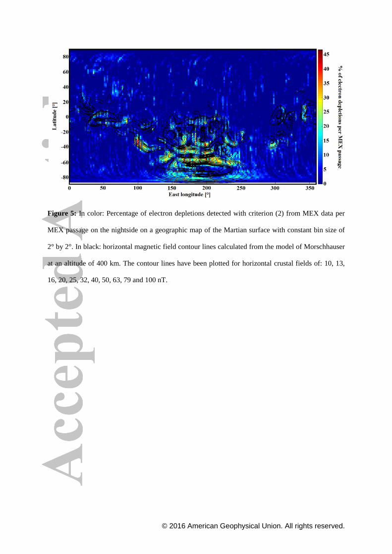
4.2. Mars EXpress

Figure 5 shows the density map of the electron depletions evaluated with criterion (2).

We chose to divide the surface of Mars into spatial bins of 2° by 2°, as there are less data

points than for MGS (Table 2). The color code corresponds to the percentage of electron

depletions per MEX passage. For each bin we calculated the ratio between the number of

time steps when an electron depletion is detected and the total number of time steps when

MEX is in the nightside with an altitude below 900 km. There are on average 500 MEX

observation time steps per bin. We have also superimposed logarithmically spaced (between

10 and 100 nT) contour lines of the horizontal crustal magnetic field calculated at 400 km

altitude from the Morschhauser model so that the maps of MEX and MGS can be compared.

As for MGS, we can see that the electron depletions are globally localized over

regions of strong horizontal crustal magnetic field. This supports the idea that, above 300

km, the main mechanism responsible for electron depletions is still the exclusion by closed

crustal magnetic loops. Some electron depletions can still be found over areas without strong

crustal magnetic field such as: [40°E, 60°N]. However, we can see on this map that the areas

with strong crustal fields located at high southern latitudes are now in a better agreement with

the distribution of electron depletions. This difference with MGS may be due to the different

ways MGS and MEX covered the Martian surface. MGS covered each latitude on the

nightside on each orbit whereas MEX periapsis only covers the southern pole during specific

periods. Thus, depending on the seasons when these periods occurred, the percentages

obtained in the southern pole region are modified.

The percentages found on Figure 5 are much lower than those found on Figure 4 with

MGS and do not enable us to analyze the presence of permanent and intermittent depletions.

However, these percentages seem quite similar to those found by Hall et al. [2016]. Using the


depletions automatically detected thanks to their criterion, Hall et al. [2016] produced an

occurrence map of the electron depletions observed with MEX during the same time period

with a resolution of 15° by 15°, in order to emphasize large scale occurrences. Their map

highlights several areas where electron depletions are concentrated which are consistent with

the ones observed on figure 5, like the regions centered on [300°E, -40°N] or [200°E, -60°N].

The two maps are comparable except for the regions centered on [200°E; -10°N] where Hall

et al. [2016] found their maximum occurrence of depletions. We here found for this region a

percentage of with no real extension toward the Northern hemisphere but rather

toward the Southern hemisphere where the maximum percentages are located, coincident

with the strongest horizontal crustal magnetic fields. Figures 5 and 4 also reveal the presence

of electron depletions in the region centered on [70°E, 80°N] where a small crustal magnetic

source exists, but which is not observed by Hall et al. [2016], maybe due to the resolution

chosen by the authors.

As was also mentioned by Hall et al. [2016], the figure 4 shows that the regions with

strong concentration of electron depletions are surrounded by regions having moderate

occurrence rate. Finally, the noise observed on figure 5 has also been detected by Hall et al.

[2016] who found a background level around 10% present all over their map. We here tend to

limit this noise by selecting events on the nightside and at altitudes below 900 km.


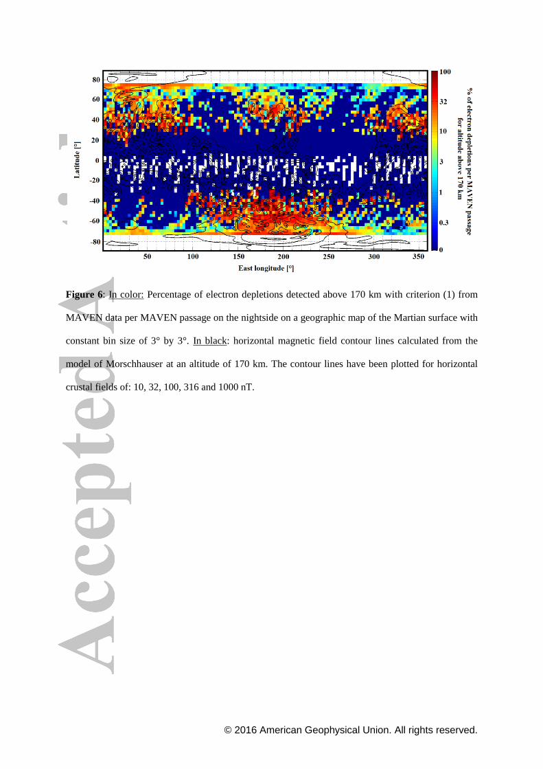
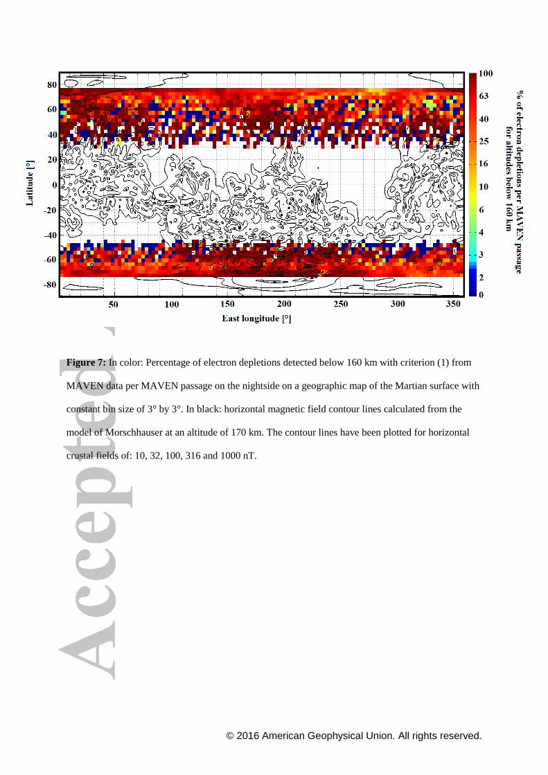
4.3. MAVEN

While MGS was at an altitude of 400 km and MEX has its lower periapsis at 245

km, MAVEN can reach altitudes down to 125 km during its „deep-dip‟ campaigns, which

enables a more comprehensive view of the electron depletion phenomenon. Figures 6 and 7

show the density maps of electron depletions detected with MAVEN. In the same way as for

the map of MGS and MEX, we calculated the number of time steps when electron depletions

are detected in spatial bins of 3° longitude by 3° latitude and divided it by the number of time

steps when MAVEN is in the nightside in each bin. Since Steckiewicz et al. [2015] showed

that the electron depletions distribution was different for altitudes below and above 160-170

km in the Northern hemisphere, we here provide two maps, the first for altitudes above 170

km and below 900 km (figure 6) and the second for altitudes below 160 km (figure 7). This

choice enable us to emphasize the differences between the distributions of electron depletions

at low and high altitudes. The density maps are superimposed with a map of the horizontal

crustal field calculated at 170 km with the Morschhauser model. The contour lines are

logarithmically spaced between 10 and 1000 nT. Larger bins of 3° by 3° have been chosen

for MAVEN as there are less data than for MEX and MGS (Table 2). On average, there are

280 time steps per bin on Figure 6 and 90 on Figure 7.

In Figure 6, for events at altitudes greater than 170 km, we found the same behavior as

for MEX and MGS: the depletions are aggregated on areas of strong horizontal crustal

magnetic fields. The variability of the percentage of electron depletions per MAVEN passage

seems to support the idea of permanent and intermittent electron depletions. Hence

percentages close to 100% are preferentially seen near the local maxima of horizontal crustal

fields whereas lower percentages are observed far from crustal magnetic field sources, which

means that electron depletions are not always present when MAVEN observes these regions.


However, as the MAVEN coverage is still not complete, we cannot affirm that permanent

depletions are surrounded by intermittent ones as it was observed on MGS distribution but we

can see a trend emerge. In Figure 7, for events at altitudes lower than 160 km, we can see that

the higher percentage of electron depletions are still localized above strong crustal magnetic

field sources but we can notice that the global distribution is far more homogeneous than for

the distribution above 170 km, regardless of the horizontal magnetic field. Thus closed

crustal magnetic loops are still an important process responsible for electron depletions.

However, there is also another important process which is involved and which does not

depend a priori on crustal magnetic field, like electron absorption by atmospheric . The

study of the Southern hemisphere of Mars confirms the fact that the distribution of electron

depletions is highly dependent on altitude.


5. Altitude dependence of electron depletions distribution

In Steckiewicz et al. [2015] we showed that the altitude distribution of electron

depletions detected by MAVEN observations in the Northern hemisphere was different above

and below a transition region near 160-170 km altitude. There were far more chances to

detect an electron depletion during a passage of MAVEN below this region than above. Here

we complement this study with data from MAVEN above the Southern hemisphere mid-

latitudes and data from MEX above both hemispheres. The time periods studied are

respectively the same as for the previous section.

5.1. Description of the method

Since the MAVEN data currently only covers latitudes northward of 20° and

southward of -20°, we only include MEX observations of the electron depletions detected in

the same range of latitudes. We have also studied the Northern and the Southern hemispheres

separately. For both spacecraft we took an altitude resolution of 2 km, which represent

10 000 MEX passages per bin and 2 600 MAVEN passages per bin on average. For each

bin we calculated the number of time steps when electron depletions are detected and the

number of time steps when the spacecraft is in the nightside. The ratio gives the percentage of

electron depletions among the spacecraft passages in each altitude bin. The MGS

observations previously discussed are not applicable to this analysis, since the spacecraft had

a circular orbit with an almost constant altitude.


5.2. Results

Figure 8 shows the percentage of electron depletions detected along the MAVEN and

MEX passages as a function of altitude. The red and green profiles correspond to

observations made by MAVEN and MEX respectively above the Southern hemisphere,

whilst the blue and black profiles correspond to observations made by MAVEN and MEX

respectively above the Northern hemisphere. We can notice that MEX data are only available

down to 307 km in the Northern hemisphere whereas they are available down to 245 km in

the Southern hemisphere. This difference is only due to MEX orbital geometry.

We can see that the MEX and MAVEN results match well between 900 and 300 km.

In this range of altitude, both datasets show that there is far more chance to detect an electron

depletion in the Southern hemisphere than in the Northern hemisphere. This phenomenon

seems to be due to the presence in the Southern hemisphere of stronger crustal magnetic

sources than in the Northern hemisphere. Hence the closed crustal magnetic loops can extend

higher in the Southern hemisphere than in the Northern. Between 300 and 245 km, even

though data are no more recorded by MEX in the Northern hemisphere, there are still some in

the Southern hemisphere. Although strong variations can be observed on MEX data, we can

see that the profile follows the trend set by MAVEN data. These variations may be due to the

range of altitudes which is beneath the nominal periapsis and hence sparsely covered by the

spacecraft.

For altitudes greater than 500 km, Hall et al. [2016] found that the normalized

occurrence of electron depletions was less than 5% across the majority of latitudes and

altitudes, except for the strongest crustal magnetic field regions around which the majority of

the events are distributed and where enhanced occurrence are then detected up to 1 000 km.


This is consistent with the results obtained on figure 8 even if the percentages are lower than

those found by Hall et al. [2016]: 1% in the Northern hemisphere and 3% in the Southern

hemisphere at 500 km. Below 500 km, the occurrence of electron depletions increases rapidly

in both studies. The main difference is that Hall et al. [2016] found that the distribution of

electron depletions becomes more homogeneous below 500 km, even if the highest

occurrences are still located above the strongest crustal magnetic field areas. On figure 8 we

clearly see that there are more electron depletions detected by MEX in the Southern

hemisphere than in the Northern hemisphere, at least until 300 km. The difference between

the two hemispheres even increases between 500 km and 300 km.

Where MEX ceases to record data, MAVEN continues to observe electron depletions

at lower altitudes. We can see that the difference in percentage between the Southern and the

Northern hemispheres persists until a transition region near 160-170 km altitude, where the

two curves join and stay close until 125 km. Hence, at low altitudes the electron depletion

distribution does not depend on the hemisphere nor on the presence of crustal magnetic

sources. This result reinforces the conclusions of Steckiewicz et al. [2015] about the presence

of two processes responsible for electron depletions, each of them being predominant in a

specific altitude regime. Depletion events above 160-170 km altitude are predominantly

produced by the exclusion of suprathermal electrons by closed crustal magnetic fields,

whereas events below 160-170 km are predominantly produced by absorption by

atmospheric . The study of the Southern hemisphere with MAVEN data also shows that

the transition between the altitude regimes seems to be the same in both hemispheres,

regardless the intensity of the crustal magnetic sources.


7. Conclusions

In this paper we have analyzed observations of electron depletions from three

different Martian missions (MGS, MEX and MAVEN) in order to better characterize their

altitude and geographical distributions and understand their formation processes. We thus

provide here the first multi-spacecraft analysis of electron depletions covering seventeen

years of Martian exploration, offering a comprehensive view of the phenomenon.

While previous studies used different approaches to identify electron depletions in

MGS and MEX data, we here used the same method to automatically detect these events in

the three Martian orbiters datasets. In addition we did not impose any geometric restrictions

in our conditional research - contrary to previous studies like the one of Hall et al. [2016]

which was restricted to the illuminated induced magnetosphere.

Our results show that electron depletions are spread on the nightside of the Martian

environment at altitudes between 110 and 900 km. For comparable altitude ranges (i.e. above

about 250 km), the aerographic distributions of electron depletions for each mission produced

results in agreement with each other and with previous studies: electron depletions are

strongly linked with the horizontal crustal magnetic fields. The study of Steckiewicz et al.

[2015] has been extended to the Southern hemisphere of Mars at low altitudes and has

confirmed this link with the crustal magnetic sources until a transition region near 160-170

km altitude regardless the hemisphere (and thus regardless the intensity of the crustal

magnetic sources). It was obviously not possible to identify this transition region with MGS

and MEX due to their altitude limitations ( 400 km for MGS and greater than 245 km for

MEX). The comparison of the altitudinal distribution of the electron depletions detected in

both hemispheres by MEX and MAVEN showed that above this transition region far more

depletions are observed above the Southern hemisphere, where the strongest crustal magnetic


field sources are located. The crustal fields thus act as a barrier preventing the replenishing of

the electron depleted area (depleted due to the absence of solar EUV photoionization) by

external incoming electrons. However, below the transition region at 160-170 km, the

MAVEN data has revealed that the distribution is globally homogeneous in latitude-longitude

and between both hemispheres. Thus at low altitudes crustal magnetic fields are no longer

predominant in the creation of electron depletions, further suggesting that the denser

atmospheric population is responsible for creating the depletions at those altitudes by

absorption processes [Steckiewicz et al., 2015].

One original application of our study is using nightside suprathermal electron

depletions as an indirect method of detecting crustal fields allowing the determination of the

topology of the magnetic field using electron spectrometers [Mitchell et al. 2005, Brain et al.

2007]. Closed magnetic field lines are indeed associated with the Martian crustal magnetic

fields and can be identified in the nightside by the presence of electron depletions notably at

altitudes above approximately 170 km.

As studied by Hall et al. [2016], electron depletions can be observed to some extent in

the terminator region. The processes creating electron depletions in regions illuminated or in

shadow could be different. The electron depletion distributions obtained in the dawn and the

dusk sector are also expected not to be the same since the photoelectrons - liberated on the

dayside of Mars mainly from ionization of atmospheric and O by solar photons - are

travelling from the dayside to the nightside following the rotation of the planet. A delay is

expected on the dusk side for the electrons to be depleted. A study of the distribution of

electron depletion with respect to local time and solar zenith angle will be made when the

complete local time coverage will be achieved by MAVEN and reported in a future paper.


Acknowledgements

This work has been supported by the French space agency CNES for the part based on

observations obtained with the SWEA instrument on MAVEN. The MAVEN project is

supported by NASA through the Mars Exploration Program. The authors acknowledge the

support of the MAVEN project and particularly of the instrument and science teams. Data

analysis was performed with the AMDA science analysis system (http://amda.cdpp.eu)

provided by the Centre de Données de la Physique des Plasmas (CDPP) supported by CNRS,

CNES, Observatoire de Paris and Université Paul Sabatier, Toulouse, France. The MGS,

MEX, and MAVEN data used in this paper are publicly available through the Planetary Data

System (http://ppi.pds.nasa.gov/). The authors sincerely thank the two anonymous reviewers

for their constructive comments.

http://ppi.pds.nasa.gov/


References

Acuña, M. H., J.E.P Connerney, P. Wasilewski, R.P. Lin, D. Mitchell, K.A. Anderson, C.W.

Carlson, J. McFadden, H. Rème, C. Mazelle, D. Vignes, S.J. Bauer, P. Cloutier and

N.F. Ness (2001), Magnetic field of Mars: Summary of results from the aerobraking

and mapping orbits, J. Geophys. Res., 106(E10), 23403-23417, doi:

10.1029/2000JE001404

Albee, A. L., R. E. Arvidson, F. Palluconi and T. Thorpe (2001), Overview of the Mars

Global Surveyor mission, J. Geophys. Res., 106(E10), 23291-23316, doi:

10.1029/2000JE001306

Andersson, L., R. E. Ergun, G. T. Delory, A. I. Eriksson, J. Westfall, H. Reed, J. McCauly,

D. Summers, and D. Meyers (2015), The Langmuir Probe and Waves instrument for

MAVEN, Space Sci. Rev., 195: 173-198, doi: 10.1007/s11214-015-0194-3

Barabash, S., Lundin, R., & Andersson, H. et al. (2004), ASPERA-3: Analyser of Space

Plasmas and Energetic Ions for Mars Express, Mars Express: the Scientific Payload

(ESA SP-1240), ed. A. Wilson & A. Chicarro (Noordwijk: ESA), 121

Bertucci, C., C. Mazelle, D. H. Crider, D. Vignes, M. H. Acuña, D. L. Mitchell, R. P. Lin, J.

E. P. Connerney, H; Rème, P. A. Cloutier, N. F. Ness, and D. Winterhalter (2003),

Magnetic field draping enhancement at the Martian magntic pileup boundary from

Mars Global Surveyor observations, Geophys. Res. Lett., 30, no. 2, 1099, doi:

10.1029/2002GL015713

Bougher, S. et al., (2015), Early MAVEN Deep Dip Campaigns: First Results and

Implications, Sciences, Vol. 350, Issue 6261, doi: 10.1126/science.aad0459

Brain, D. A., F. Bagenal, M. H. Acuña, and J. E. P. Connerney (2003), Martian magnetic

morphology: Contributions from the solar wind and crust, J. Geophys. Res., 108(A12),

1424, doi: 10.1029/2002JA009482


Brain, D. A., R.J. Lillis, D.L. Mitchell, J. S. Halekas, and R. P. Lin (2007), Electron pitch

angle distributions as indicators of magnetic field topology near Mars, J. Geophys.

Res., 112(A09201), doi: 10.1029/2007JA012435

Chicarro, A., P. Martin, and R. Trautner (2004), The Mars Express Mission: An overview,

Planetary Missions Division, Research & Scientific Support Department,

ESA/ESTEC, PO box 299, 2200 AG Noordwijk, The Netherlands

Connerney, J. E. P., J. Espley, P. Lawton, S. Murphy, J. Odom, R. Oliverson, and D.

Sheppard (2015), The MAVEN magnetic field investigation, Space Sci. Rev.,

doi:10.1007/s11214-015-0169-4.

Duru, F., D. A. Gurnett, D. D. Morgan, J. D. Winningham, R. A. Frahm, and A. F. Nagy

(2011), Nightside ionosphere of Mars studied with local electron densities: A general

overview and electron density depressions, J. Geophys. Res., 116(A10316), doi:

10.1029/2011JA016835

Fillingim, M. O., L. M. PetiColas, R. J. Lillis, D. A. Brain, J. S. Halekas, D. Lummerzheim,

and S. W. Bougher (2010), Localized ionization patches in the nighttime ionosphere

of Mars and their electrodynamic consequences, Icarus, 206(112-119), doi:

10.1016/j.icarus.2009.03.005

Frahm, R. A., et al. (2006), Locations of atmospheric photoelectron energy peaks within the

Mars environment, Space Sci. Rev., 126: 389-402, doi: 10.1007/s11214-006-9119-5

Fränz, M., E. Dubinin, E. Roussos, J. Woch, J. D. Winningham, R. Frahm, A. J. Coates, A.

Fedorov, S. Barabash, and R. Lundin (2006), Plasma moments in the environment of

Mars, Mars Express ASPERA-3 Observations, Space Sci. Rev., 126(165-207), doi:

10.1007/s11214-006-9115-9


Fränz, M., E. Dubinin, E. Nielsen, J. Woch, S. Barabash, R. Lundin, and A. Fedorov (2010),

Transterminator ion flow in the Martian ionosphere, Planet. Space Sci., 58(1442-

1454), doi: 10.1016/j.pss.2010.06.009

Hall, B. E. S., M. Lester, J. D. Nichols, B. Sánchez-Cano, D. J. Andrews, H. J. Opgenoorth,

M. Fränz (2016), A survey of suprathermal electron flux depressions, or „electron

holes‟, within the illuminated Martian induced magnetosphere, J. Geophys. Res., doi:

10.1002/2015JA021866

Itikawa, Y. (2002), Cross sections for electron collisions with carbon dioxide, J. Phys. Chem.

Ref. Data, Vol. 31, No. 3, doi: 10.1063/1.1481879

Jakosky, B. M., J. M. Grebowsky, J. G. Luhmann, and D. A. Brain (2015), Initial results from

the MAVEN mission to Mars, Geophys. Res. Lett., 42 8791-8802, doi:

10.1002/2015GL065271

Krasnopolsky, V. A. (2002, Mars‟ upper atmosphere and ionosphere at low, medium and

high solar activities: Implications for evolution of water, J. Geophys. Res., 107(E12),

5128, doi: 10.1029/2001JE001809

Lillis, R. J., H. V. Frey, and M. Manga (2008), Rapid decrease in Martian crustal

magnetization in the Noachian era: Implications for the dynamo and climate of early

Mars, Geophys. Res. Lett., 35, L14203, doi: 10.1029/2008GL034338

Lillis, R. J., M. O. Fillingim, and D. A. Brain (2011) Three-dimensional structure of the

Martian nightside ionosphere: Predicted rates of impact ionization from Mars Global

Surveyor magnetometer and electron reflectometer measurements of precipitating

electrons, J. Geophys. Res., 116(A12317), doi: 10.1029/2011JA016982

Lillis, R. J. and D. A. Brain (2013), Nightside electron precipitation at Mars: Geographic

variability and dependence on solar wind conditions, J. Geophys. Res., 118(3546-

3556), doi: 10.1002/jgra.50171


Lillis, R. J., S. Robbins, M. Manga, J. Halekas, and H. V. Frey (2013), Time history of the

Martian dynamo from crater magnetic field analysis, J. Geophys. Res., 118(1488-

1511), doi: 10.1002/jgre.20105

Ma, Y., X. Fang, C. T. Russell, A. F. Nagy, G. Toth, J. G. Luhmann, D. A. Brain, C. Dong

(2014), Effects of crustal field rotation on the solar wind plasma interaction with

Mars, Geophys. Res. Lett., 41 (19), 6563-6569, doi: 10.1002/2014GL060785

McFadden, J. P., et al. (2015), MAVEN SuparThermal and Thermal Ion Composition

(STATIC) Instrument, Space Sci. Rev., 195(1-4) 199-256, doi: 10.1007/s11214-015-

0175-6

Mitchell, D.L., et al. (2016), The MAVEN Solar Wind Electron Analyzer, Space Sci. Rev.,1-

34 doi: 10.1007/s11214-015-0232-1

Mitchell, D. L., R.P. Lin, C. Mazelle, H. Rème, P. A. Cloutier, J. E. P. Connerney, M. H.

Acuña, and N. F. Ness (2001), Probing Mars‟ crustal magnetic field and ionosphere

with the MGS Electron reflectometer, J. Geophys. Res., 106(E10), 23419-23427, doi:

10.1029/2000JE001435

Morschhauser, A., V. Lesur and M. Grott (2014), A spherical harmonic model of the

lithospheric magnetic field of Mars, J. Geophys. Res. Planets, 119, 1162-1188, doi:

10.1002/2013JE004555

Nagy, A.F., et al. (2004), The plasma environnement of Mars, Space Sci. Rev., 111, 33-114,

doi: 10.1023/B:SPAC.0000032718.47512.92

Němec, F., D. D. Morgan, D. A. Gurnett, and F. Duru (2010), Nightside ionosphere of Mars:

Radar soundings by the Mars Express spacecraft, J. of Geophys. Res., 115, E12009,

doi: 10.1029/2010JE003663

Soobiah, Y., et al. (2006), Observations of magnetic anomaly signatures in Mars Express

ASPERA-3 ELS data, Icarus, 182(396-405), doi: 10.1016/j.icarus.2005.10.034


Steckiewicz, M., et al. (2015), Altitude dependence of nightside Martian suprathermal

electron depletions as revealed by MAVEN observations, Geophys. Res. Lett., 42,

8877-8884, doi: 10.1002/2015GL065257

Withers, P., M. O. Fillingim, R. J. Lillis, B. Häusler, D. P. Hinson, G. L. Tyler, M. Pätzold,

K. Peter, S. Tellmann, and O. Witasse (2012), Observations of the nightside

ionosphere of Mars by the Mars Express Radio Science Experiement (MaRS), J.

Geophys. Res., 117(A12307), doi: 10.1029/2012JA018185

Ulusen, D., and I. R. Linscott (2008), Low-energy electron current in the Martian tail due to

reconnection of draped interplanetary magnetic field and crustal magnetic fields, J.

Geophys. Res., 113, E06001, doi: 10.1029/2007JE002916

Zhang, M. H. G., J. G. Luhmann, A. J. Kliore (1990), An observational study of the nightside

ionospheres of Mars and Venus with radio occultation methods, J. Geophys. Res.,

95(A10), (17095-17102) doi: 10.1029/JA095iA10p17095


Table1. Summary of the characteristics of the magnetometer, electron spectrometer, ion spectrometer

and Langmuir probe onboard MGS, MEX and MAVEN

Instrument Type Quantity MGS MEX MAVEN

Magnetometer Magnitude range 4 – 65536 nT none 0.06 - 65536 nT

Electron

spectrometer

Energy range 10 – 20000 eV 1 – 20000 eV 3 – 4600 eV

Energy resolution 25% 8% 17%

Ion spectrometer

Energy range

none

10-30000 eV/q 0.1-30000 eV/q

Energy resolution 7% 16%

Mass range

1, 2, 4, 8, 16

and >20 m/q

Langmuir probe Temperature none none 0.05 to 5 eV


Table 2. For each mission are reported here the number of orbits under study (for MEX it corresponds

to the number of time intervals longer than one hour when ELS was in the survey mode. It

corresponds approximately to the number of orbits studied), the number of depletions detected by

criterion (3) for MGS, criterion (2) for MEX and criterion (1) for MAVEN, the number of orbits

containing depletions and the median number of depletions per orbit.

MGS MEX MAVEN

Number of orbits under study 42 048 9 983 2 138

Number of depletions detected 116 278 14 517 3 698

Number of orbits containing depletions 29 460 2 197 899

Median number of depletions per orbit 4 5 4


Figure 1. Example of electron depletion observed by MGS on April 26, 2005. First panel: ER energy-

time spectrogram of omnidirectional electron flux. Second panel: ER omnidirectional electron flux

summed over all energies available [11-16127 eV]. Third panel: Detection of electron depletions by

criterion (3) (black boxes). See section 3 for more details. The shadow corresponds to the nightside.

Fourth panel: Magnetic field intensity (measured by MAG in black and calculated from the model of

Morschhauser in blue). Fifth panel (bottom right): MGS orbital trajectory in a cylindrically symmetric

MSO coordinates frame. The location of the electron depletions detected are highlighted in red. The

altitude is defined with respect to a sphere with the Mars‟ volumetric mean radius of 3389.51 km.


Figure 2. Example of electron depletion observed by MEX on June 23, 2012. First panel: ELS

energy-time spectrogram of omnidirectional electron counts per second. Second panel: ELS electron

counts per second summed over all the energies available (1-21177 eV). Third panel: Detection of

electron depletions by criterion (2) (black boxes). See section 3 for more details. The shadow

corresponds to the nightside. Fourth panel: IMA energy-time spectrogram of omnidirectional heavy

ions counts per second (m/q>20). Fifth panel: Magnetic field intensity calculated from the

Morschhauser model. Sixth panel (bottom right): MEX orbital trajectory in a cylindrically symmetric

MSO coordinates frame. The location of the electron depletions detected are highlighted in red.


Figure 3. Example of electron depletion observed with MAVEN. First panel: SWEA energy-time

spectrogram of omnidirectional electron energy flux (ENGY mode) corrected for the potential

measured with LPW. Second panel: Electron density calculated with SWEA (black) superimposed

with the density calculated with LPW (red). Third panel: Detection of electron depletions by criterion

(1) (black boxes). See section 3 for more details. The shadow corresponds to the nightside. Fourth

panel: STATIC energy-time spectrogram of omnidirectional ion energy flux (C0 mode). Fifth panel:

STATIC mass-time spectrogram of omnidirectional ion energy flux (C6 mode). Sixth panel: Magnetic

field intensity (measured by MAG in black and calculated from the model of Morschhauser in red).

Seventh panel (bottom right): MAVEN orbital trajectory in a cylindrically symmetric MSO

coordinates frame. The location of the electron depletions detected have been highlighted in red.


Figure 4. In color: Percentage of electron depletions detected with criterion (3) from MGS data per

MGS passage on the nightside on a geographic map of the Martian surface with constant bin size of

1° by 1°. In black: horizontal magnetic field contour lines calculated from the model of Morschhauser

at an altitude of 400 km. The contour lines have been plotted for horizontal crustal fields of: 10, 13,

16, 20, 25, 32, 40, 50, 63, 79 and 100 nT.


Figure 5: In color: Percentage of electron depletions detected with criterion (2) from MEX data per

MEX passage on the nightside on a geographic map of the Martian surface with constant bin size of

2° by 2°. In black: horizontal magnetic field contour lines calculated from the model of Morschhauser

at an altitude of 400 km. The contour lines have been plotted for horizontal crustal fields of: 10, 13,

16, 20, 25, 32, 40, 50, 63, 79 and 100 nT.


Figure 6: In color: Percentage of electron depletions detected above 170 km with criterion (1) from

MAVEN data per MAVEN passage on the nightside on a geographic map of the Martian surface with

constant bin size of 3° by 3°. In black: horizontal magnetic field contour lines calculated from the

model of Morschhauser at an altitude of 170 km. The contour lines have been plotted for horizontal

crustal fields of: 10, 32, 100, 316 and 1000 nT.


Figure 7: In color: Percentage of electron depletions detected below 160 km with criterion (1) from

MAVEN data per MAVEN passage on the nightside on a geographic map of the Martian surface with

constant bin size of 3° by 3°. In black: horizontal magnetic field contour lines calculated from the

model of Morschhauser at an altitude of 170 km. The contour lines have been plotted for horizontal

crustal fields of: 10, 32, 100, 316 and 1000 nT.


Figure 8. Percentages of electron depletions detected by criterion (1) among MAVEN passages (in

blue and red) and by criterion (2) among MEX passages (in black and green) calculated in bins of 2

km altitude. The red and green lines correspond to depletions observed in the Southern hemisphere

and red and black lines correspond to depletions detected in the Northern hemisphere.

comparative study of the martian suprathermal electron...

Documents