comparative study of growth and productivity of …
TRANSCRIPT

COMPARATIVE STUDY OF GROWTH ANDPRODUCTIVITY OF MAIZE (Zea mays L.)UNDER DIFFERENT JHUM CYCLES OF
MIZORAM
THESISSubmitted in partial fulfillment of the requirements
for the degree ofDOCTOR OF PHILOSOPHY IN FORESTRY
By
LALRAMMUANPUIA HNAMTEMZU/PhD/279 of 09.06.2009
Department of Forestry,School of Earth Sciences & Natural Resources Management
Mizoram University,Aizawl -796004
2016

MIZORAM UNIVERSITYAIZAWL – 796004, MIZORAMDEPARTMENT OF FORESTRY
CERTIFICATE
This is to certify that the thesis entitled “ Comparative Study of Growth and
Productivity of Maize (Zea mays L.) Under Different Jhum Cycles in Mizoram”
submitted by Mr. Lalrammuanpuia Hnamte for the degree of Doctor of Philosophy in
Forestry embodies the record of original investigation carried out by him under my
guidance and supervision. He has been duly registered and the thesis presented is
worthy of being considered for the award of the Ph.D degree. This thesis or any part
thereof has not been submitted for any degree of any other University.
Date: Mizoram University (Prof. B. GOPICHAND)
Supervisor
_______________________

MIZORAM UNIVERSITYAIZAWL – 796004, MIZORAMDEPARTMENT OF FORESTRY
DECLARATION
I, Mr. Lalrammuanpuia Hnamte, hereby declare that the subject matter of this
thesis is the record of the work done by me, that the contents of this thesis did not
form basis for the award of any previous degree to me or to anybody else, and the
thesis has not been submitted by me for any research degree in any other University/
Institution.
This is being submitted to the Mizoram University for the degree of Doctor of
Philosophy in Forestry.
(LALRAMMUANPUIA HNAMTE)
Candidate
(Dr. S.K. Tripathi) (Prof. B. GOPICHAND)
Head Supervisor
CONTENTS
Page No.
Acknowledgement i
List of Tables ii - iv
List of figures v - viii
List of Photo Plates ix
List of Abbreviations used x
Chapter 1 Introduction 1 - 45
Chapter 2 Review of Literature 46 -79
Chapter 3 Study Area 80 - 87
Chapter 4 Materials and Methods 88 - 98
Chapter 5 Results 99 - 150
Chapter 6 Discussion 151 - 157
Chapter 7 Summary and Conclusions 158 - 160
References 161 - 192

ACKNOWLEDGEMENTS
I express my heartfelt gratitude to my supervisor Prof. B. Gopichand,Department of Forestry, Mizoram University, Aizawl for his benevolentguidance and advice throughout the course of the study. Without him, thisresearch work will not be completed.
I thank Dr. S.K.Tripathi, Head, Department of Forestry and otherfaculty members for their support during my research tenure.
My deepest thanks goes to Dr. C. Lalrammawia, for helping meanalyze my data and in shaping up my thesis. The never endingencouragement, endless support and immeasurable help from you and yourfamily is appreciated.
I am also thankful to the Principal and Staffs of Mizoram Institute ofComprehensive Education, Venghlui, Aizawl for giving me the time needed tocomplete my PhD.
I acknowledge Dr. David C. Vanlalfakawma for his valuable inputs inthe analysis of my research data.
I am indebted to my relatives for their untiring help, particularly inlocating experimental sites and in collecting data. Your encouragement andinvolvement from the get-go is vital for the completion of this work.
I owe much to my wife for her unwavering and diligent support. I alsoextend my deepest gratitude to my parents for their prayers, inspiration andconstant motivation. A simple thank you is insufficient.
I thank my friends and well wishers who have always helped at theappropriate time.
Most of all, I thank the Almighty God for bestowing countlessblessings and for granting me strength and opportunity to carry out thisresearch from the beginning till its completion.
Dated the ………., 2016. (LALRAMMUANPUIA HNAMTE )
i
LIST OF TABLES
Table 1.1 Composition per 100g of edible portion of maize (dry).
Table 1.2 Top ten maize producers in 2013 (FAOSTAT 2014).
Table 4.1 Table showing combination of spacing and fertilizer treatment plots.
Table 5.1 Monthly rainfall of 2010 showing the rainfall pattern during theexperimental period.
Table 5.2 Soil properties of 2JC, 3JC and 5JC before land preparation.
Table 5.3.1 Plant height at 15 days after sowing (DAS) under different spacing andfertilizer application levels in 2, 3 and 5 years jhum cycles. Mean± SEM.
Table 5.3.2 Plant height at 30 days after sowing (DAS) under different spacing andfertilizer application levels in 2, 3 and 5 years jhum cycles. Mean± SEM.
Table 5.3.3 Plant height at 45 days after sowing (DAS) under different spacing andfertilizer application levels in 2, 3 and 5 years jhum cycles. Mean± SEM.
Table 5.3.4 Plant height at 60 days after sowing (DAS) under different spacing andfertilizer application levels in 2, 3 and 5 years jhum cycles. Mean± SEM.
Table 5.3.5 No. of leaves at 15 days after sowing (DAS) under different spacingand fertilizer application levels in 2, 3 and 5 years jhum cycles. Mean± SEM.
Table 5.3.6 No. of leaves at 30 days after sowing (DAS) under different spacingand fertilizer application levels in 2, 3 and 5 years jhum cycles. Mean± SEM.
Table 5.3.7 No. of leaves at 45 days after sowing (DAS) under different spacingand fertilizer application levels in 2, 3 and 5 years jhum cycles. Mean± SEM.
Table 5.3.8 No. of leaves at 60 days after sowing (DAS) under different spacingand fertilizer application levels in 2, 3 and 5 years jhum cycles. Mean± SEM.
Table 5.3.9 Biomass at maturity harvest under different spacing and fertilizerapplication levels in 2, 3 and 5 years jhum cycles. Mean± SEM.
ii

Table 5.4.1 Length of cob under different spacing and fertilizer application levelsin 2, 3 and 5 years jhum cycles. Mean± SEM.
Table 5.4.2 No. of Kernel rows per cob under different spacing and fertilizerapplication levels in 2, 3 and 5 years jhum cycles. Mean± SEM.
Table 5.4.3 The effect of fertilizer application on number of Kernels per row underS1, S2 and S3 spacing in 2, 3 and 5 years jhum cycles. Mean± SEM.
Table 5.4.4 The effect of fertilizer application on number Kernels per cob underS1, S2 and S3 spacing in 2, 3 and 5 years jhum cycles. Mean± SEM.
Table 5.4.5 Test weight (wt. of 1000 grains) under different spacing and fertilizerapplication levels in 2, 3 and 5 years jhum cycles. Mean± SEM.
Table 5.4.6 Grain yield under different spacing and fertilizer application levels in2, 3 and 5 years jhum cycles. Mean± SEM.
Table 5.4.7 Harvest Index under different spacing and fertilizer application levelsin 2, 3 and 5 years jhum cycles. Mean± SEM.
Table 5.5.1 Effect of spacing on plant height at 15 days after sowing (DAS)under different levels of fertilizer applications in 2, 3 and 5 years jhumcycles. Mean± SEM.
Table 5.5.2 Effect of spacing on plant height at 30 days after sowing (DAS)under different levels of fertilizer applications in 2, 3 and 5 years jhumcycles. Mean± SEM.
Table 5.5.3 Effect of spacing on plant height at 45 days after sowing (DAS)under different levels of fertilizer applications in 2, 3 and 5 years jhumcycles. Mean± SEM.
Table 5.5.4 Effect of spacing on plant height at 60 days after sowing (DAS)under different levels of fertilizer applications in 2, 3 and 5 years jhumcycles. Mean± SEM.
Table 5.5.5 Effect of spacing on number of leaves per plant at 15 days after sowing(DAS) under different levels of fertilizer applications in 2, 3 and 5years jhum cycles. Mean± SEM.
Table 5.5.6 Effect of spacing on number of leaves per plant at 30 days after sowing(DAS) under different levels of fertilizer applications in 2, 3 and 5years jhum cycles. Mean± SEM.
Table 5.5.7 Effect of spacing on number of leaves per plant at 45 days after sowing(DAS) under different levels of fertilizer applications in 2, 3 and 5years jhum cycles. Mean± SEM.
iii

Table 5.5.8 Effect of spacing on number of leaves per plant at 60 days after sowing(DAS) under different levels of fertilizer applications in 2, 3 and 5years jhum cycles. Mean± SEM.
Table 5.5.9 Effect of spacing on biomass production at maturity harvest underdifferent levels of fertilizer applications in 2, 3 and 5 years jhumcycles. Mean± SEM.
Table 5.6.1 Effect of spacing on length of cob under different levels of fertilizerapplications in 2, 3 and 5 years jhum cycles. Mean± SEM.
Table 5.6.2 Effect of spacing on kernel rows per cob under different levels offertilizer applications in 2, 3 and 5 years jhum cycles. Mean± SEM.
Table 5.6.3 Effect of spacing on kernel per row under different levels of fertilizerapplications in 2, 3 and 5 years jhum cycles. Mean± SEM.
Table 5.6.4 Effect of spacing on kernel per cob under different levels of fertilizerapplications in 2, 3 and 5 years jhum cycles. Mean± SEM.
Table 5.6.5 Effect of spacing on test weight (1000 grain wt.) under different levelsof fertilizer applications in 2, 3 and 5 years jhum cycles. Mean± SEM.
Table 5.6.6 Effect of spacing on grain yield under different levels of fertilizerapplications in 2, 3 and 5 years jhum cycles. Mean± SEM.
Table 5.6.7 Effect of spacing on Harvest Index (HI) under different levels offertilizer applications in 2, 3 and 5 years jhum cycles. Mean± SEM.
iv
LIST OF FIGURES
Fig. 3.1 Map of the districts in Mizoram State showing the location ofAizawl city.
Fig. 3.4 Map of Mizoram State showing open and dense forest. (ISFR, 2011)
Fig. 4.1 Location of the experimental site at Edenthar showing the treatmentplots of the experimental block.
Fig. 5.3.1 Effect of fertilizer application on plant height at 15 DAS under differentspacing in 2 years, 3 years and 5 years jhum cycles.
Fig. 5.3.2 Effect of fertilizer application on plant height at 30 DAS under differentspacing in 2 years, 3 years and 5 years jhum cycles.
Fig. 5.3.3 Effect of fertilizer application on plant height at 45 DAS under differentspacing in 2 years, 3 years and 5 years jhum cycles.
Fig. 5.3.4 Effect of fertilizer application on plant height at 60 DAS under differentspacing in 2 years, 3 years and 5 years jhum cycles.
Fig. 5.3.5 Effect of fertilizer application on number of leaves per plant at 15 DASunder different spacing in 2 years, 3 years and 5 years jhum cycles.
Fig. 5.3.6 Effect of fertilizer application on number of leaves per plant at 30 DASunder different spacing in 2 years, 3 years and 5 years jhum cycles.
Fig. 5.3.7 Effect of fertilizer application on number of leaves per plant at 45 DASunder different spacing in 2 years, 3 years and 5 years jhum cycles.
Fig. 5.3.8 Effect of fertilizer application on number of leaves per plant at 60 DASunder different spacing in 2 years, 3 years and 5 years jhum cycles.
Fig. 5.3.9 Effect of fertilizer application on biomass production at maturityharvest under different spacing in 2 years, 3 years and 5 years jhum cycles.
Fig. 5.4.1 Effect of fertilizer application on length of cob under different spacing in2 years, 3 years and 5 years jhum cycles.
Fig. 5.4.2 Effect of fertilizer application on kernel rows per cob under different spacingin 2 years, 3 years and 5 years jhum cycles.
Fig. 5.4.3 Effect of fertilizer application on kernels per row under different spacing in2 years, 3 years and 5 years jhum cycles.
v

Fig. 5.4.4 Effect of fertilizer application on kernels per cob under different spacing in2 years, 3 years and 5 years jhum cycles.
Fig. 5.4.5 Effect of fertilizer application on test weight under different spacing in2 years, 3 years and 5 years jhum cycles.
Fig. 5.4.6 Effect of fertilizer application on grain yield under different spacing in2 years, 3 years and 5 years jhum cycles.
Fig. 5.4.7 Effect of fertilizer application on harvest index under different spacing in2 years, 3 years and 5 years jhum cycles.
Fig. 5.5.1 Effect of spacing on plant height at 15 DAS under different fertilizerapplication levels in 2 years, 3 years and 5 years jhum cycles.
Fig. 5.5.2 Effect of spacing on plant height at 30 DAS under different fertilizerapplication levels in 2 years, 3 years and 5 years jhum cycles.
Fig. 5.5.3 Effect of spacing on plant height at 45 DAS under different fertilizerapplication levels in 2 years, 3 years and 5 years jhum cycles.
Fig. 5.5.4 Effect of spacing on plant height at 60 DAS under different fertilizerapplication levels in 2 years, 3 years and 5 years jhum cycles.
Fig. 5.5.5 Effect of spacing on number of leaves per plant at 15 DAS underdifferent fertilizer application levels in 2 years, 3 years and 5 yearsjhum cycles.
Fig. 5.5.6 Effect of spacing on number of leaves per plant at 30 DAS underdifferent fertilizer application levels in 2 years, 3 years and 5 yearsjhum cycles.
Fig. 5.5.7 Effect of spacing on number of leaves per plant at 45 DAS underdifferent fertilizer application levels in 2 years, 3 years and 5 yearsjhum cycles.
Fig. 5.5.8 Effect of spacing on number of leaves per plant at 60 DAS underdifferent fertilizer application levels in 2 years, 3 years and 5 yearsjhum cycles.
Fig. 5.5.9 Effect of spacing on biomass production at maturity harvest underdifferent fertilizer application levels in 2 years, 3 years and 5 yearsjhum cycles.
Fig. 5.6.1 Effect of spacing on length of cob under different fertilizer applicationlevels in 2 years, 3 years and 5 years jhum cycles.
Fig. 5.6.2 Effect of spacing on kernel rows per cob under different fertilizerapplication levels in 2 years, 3 years and 5 years jhum cycles.
vi

Fig. 5.6.3 Effect of spacing on kernels per row under different fertilizerapplication levels in 2 years, 3 years and 5 years jhum cycles.
Fig. 5.6.4 Effect of spacing on kernels per cob under different fertilizerapplication levels in 2 years, 3 years and 5 years jhum cycles.
Fig. 5.6.5 Effect of spacing on test weight under different fertilizer applicationlevels in 2 years, 3 years and 5 years jhum cycles.
Fig. 5.6.6 Effect of spacing on grain yield under different fertilizer applicationlevels in 2 years, 3 years and 5 years jhum cycles.
Fig. 5.6.7 Effect of spacing on harvest index under different fertilizer applicationlevels in 2 years, 3 years and 5 years jhum cycles.
vii
LIST OF PHOTOPLATES
Plate 1 Experimental site at Edenthar locality showing plot-wise demarcation.
Plate 2 Growth performance of different spacing and fertilizer applicationplots of 2 years jhum cycle.
Plate 3 Growth difference between S1F0 and S3F3 plots of 3 years jhumcycles at 30 DAS.
Plate 4 Mimpui maize of S2F3 plot (120:60:40 NPK kg/ha; 60cm x 25cmspacing) at 45 DAS in 5 years jhum cycle.
Plate 5 Taking growth measurement at 60 DAS on S2F2 plot of 5 years jhumcycle.
Plate 6 S1F0 plot (55cm x 20cm spacing; no fertilizer application) of 2 yearsjhum cycle at the same time of silking stage.
Plate 7 Cobs of Mimpui maize growth under S3F3 (75cm x 20cm spacing;120:60:40 NPK kg/ha application) in 5 years jhum cycles.
Plate 8 Weighing of harvested grains for measurement of grain yield per plantand test weight.
viii
LIST OF ABBREVIATIONS USED
oC : Degree Celcius
% : per cent
cm : centimeter
E : East
Ed: (eds.) : Edition: editor(s) or edited
et al. : et alii: and others
etc. : etcetera or cetera: and the others
g/gms : gram(s)
ha : hectare
K : Potassium
m : metrum: metre
mg : milligram
mm : millimetrum: millimeter
ml : milliliter
N : North / Nitrogen
no. : numero: number
p., pp. : pigina: page, pages
P : Phosphorus
qt : quintal
sp., spp : species (singular); species (plural)
ix

1
Chapter – I
INTRODUCTION
1.1 Global Agriculture production
Agriculture is the world’s largest use of land, occupying about 38% of
the Earth’s terrestrial surface. The agricultural community has had tremendous
successes in massively increasing world food production over the past five decades
and making food more affordable for the majority of the world’s population, despite a
doubling in population (Dobermann and Nelson, 2013).
Approximately 790 million people in developing countries are
described as undernourished, with Sub-Saharan Africa highlighted as the region
with the greatest hunger (<1260kJ/ day) affecting 180 million people (FAO, 2002).
Even more troubling is the fact that thousands die daily as a result of diseases from
which they likely would have survived had they received adequate food and nutrition
(Craig D. Idso, 2011). The number of undernourished increased in the rest of East
Asia (excluding China) and even more in the rest of South Asia (excluding India)
(FAO 2006).
By 2025, continuing population growth and current agricultural
practices will lead to 36 more countries (pop. 1.4 billion) falling into the category
currently occupied by 21 countries (pop. 600 million) where either good cropland or
fresh water are scarce (National Intelligence Council. 2008). Credible research
already makes it clear that there is a growing depletion of the key natural resources,
including land, water, and biodiversity, that are fundamental for sustainable
2
production. No human endeavour uses more of these resources than agriculture.
(OECD, 2011).
Of the world’s 1.1 billion extremely poor people, about 74 % (810
Million) live in marginal areas and rely on small scale agriculture. While the world
currently produces enough food to feed everyone, at least one billion people remain
food insecure (FAO, 2010). Although the incidence of hunger dropped from a ratio of
one in three in 1960 to affecting roughly one in seven people by the 1990s, the trend
reversed in the 1990s and the absolute number of people blighted by hunger continues
to grow. In 2009, for the first time in history the population considered to be
malnourished exceeded one billion people Sub-Saharan Africa has the highest
proportion of undernourished people, 30 percent in 2010, while the Asia Pacific
region has the most undernourished people (578 million) according to the FAO. Two
thirds of the world's undernourished live in just seven countries – Bangladesh, China,
the Democratic Republic of Congo, Ethiopia, India, Indonesia and Pakistan (FAO,
2010).
It is also estimated that by 2050 another 2.3 billion people will be
added to the current population of 7 billion, with most of this increase happening in
countries that are home to significant numbers of people suffering from food
insecurity, malnutrition, and extreme poverty (2010 Revision of World Population
Prospects. U.N. Population Division of the Department of Economic and Social
Affairs).
The Green Revolution made available a package of biochemical inputs
(HYVs, fertilizer and irrigation) that promised to be scale neutral and thus raise the
yields and incomes of all farmers and substantial Government subsidies allowed

3
increased production through crop intensification (Bernstein et al., 1992). While
there is little doubt that the Green Revolution enabled massive increases in yields
and the achievement of self-sufficiency in grains for India, it had a very uneven
impact on regions, crops, and individuals (Lipton and Longhurst, 1989). Rural people
take part in a number of strategies, including agricultural intensification, migration
and livelihood diversification, which enable them to attain a sustainable livelihood
(Tiffen et al., 1994).
Productivity increase has been particularly strong in developing
countries, and especially for cereals such as rice in Asia, wheat in irrigated and
favourable production environments worldwide, and maize in Mesoamerica and
selected parts of Africa and Asia (Pingali and Heisey, 2001). Most of the world
irrigated agriculture today is in developing countries. Nearly one half of the irrigated
area of the developing countries is in India and China. Food consumption, in terms of
kcal/person/day, is the key variable used for measuring and evaluating the evolution
of the world food situation (Alexandratos and Bruinsma, 2012). Food production is
particularly sensitive to climate change, since crop yields depend in large part on
climate conditions such as temperature and rainfall patterns (Stern, 2007).
The increased food production will also have to occur on less available
arable land and this can only be accomplished by intensifying production which must
be done in an environmentally safe manner through ecological intensification.
Commercial fertilizer is responsible for 40% to 60% of the world’s food production.
So, effective and efficient use of fertilizers is very important to increase the supply of
food demand (Roberts, 2009).

4
Future word populations will require ever-increasing food supplies.
The availability of food per capita has been declining for nearly two decades, based
on available cereal grains. Cereal grains make up 80% of the world’s food. Although
grain yields per hectare in both developed and developing countries are still
increasing, these increases are slowing while the world population continues to
escalate (PRB, 2002). Although agricultural productivity has generally increased
globally, it has hardly kept the pace with population growth. In much of the
developing world, population growth has negatively impacted food security.
(Ramankutty et al., 2002).
Grains such as rice, wheat, and maize account for about half of human
caloric intake (FAO. 2002). About half of the world’s grain is now used to produce
animal feed and animal consumption is projected to double between 2000 and 2050
(Steinfield et al., 2010). A change in the availability of grains has an effect on the
food available for a large part of the human population (Yotopoulos, 1985). The vast
majority of the world’s farmers are smallholders and small farms are at risk. A trend
toward the dominance of larger farms is occurring in some countries even as
fragmentation and population growth is leading to ever smaller and perhaps
unsustainable farms in others.
Agricultural growth contributes directly to food security. It also supports
poverty reduction. The population increase, combined with moderately high income
growth, could result in a more than 70% increase in demand for food and other
agricultural products by 2050. Much of this growth originated in developing countries
(3.4 – 3.8 percent p.a.). Even though the value of total agricultural output per capita

5
has had a yearly growth of 0.6% p.a. since 1961, not all regions have followed the
same trend (Wik et al., 2008).
A trend of increasing urbanization is detected worldwide (Mitlin,
2005) which is proceeding at a high pace is an important factor influencing
consumers’ preferences (MEA, 2005). This affects food consumption patterns in a
number of ways (Regmi and Dyck, 2001). Globally, urbanization is expected to
double the proportion of urban residents to the total population, reaching nearly four
billion by 2020 and affecting mainly developing countries (Haddad et al., 1999;
Regmi and Dyck, 2001). Global trade in food and feed crops has accelerated over the
period (Galloway et al., 2007) and higher income levels are associated with a greater
demand for more expensive sources of calories, such as meat, fruit, vegetables, and
processed food products (Seale et al., 2003)
1.2 INCREASE IN AGRICULTURAL LAND AND ITS EFFECTS ON
DEFORESTATION
Forests cover almost one third of the earth’s land surface
providing many environmental benefits including a major role in the hydrologic cycle,
soil conservation, prevention of climate change and preservation of biodiversity
(Sheram, 1993). Deforestation including clearing for agricultural activities is often the
only option available for the livelihoods of farmers living in forested areas (Angelsen,
1999). A global move to sustainable agriculture for sustainable development is clearly
vital (Munasinghe and Swart, 2005). Land conversion from forests to agriculture and
pasture has been associated with climate changes at the global scale (Fearnside,
1996). While developed countries have contributed to much of the planet’s recent

6
warming trend by burning fossil fuels and via the introduction of industrial
compounds. Adger and Brown (1994) estimated that tropical deforestation is
responsible for between 25% and 30% of the purported climate warming in the world;
and forests are responsible for about 90% of the carbon stored in global vegetation
(Dale, 1997). Furthermore, climate change is believed to affect world food supply and
productivity (Brown, 1994).
The practice of jhum cultivation is reported to account for 60%
forest losses worldwide each year (Lele et al., 2008). The ever increasing population
has created tremendous pressure on land to provide basic requirement for survival. To
meet these requirements, the limited natural resources are being over-exploited
resulting in widespread ecosystem degradation (Grogan et al., 2012). Grazing land
and land for crops to feed animals, makes up 80% of all agricultural land – 3.4 billion
hectares for grazing and 0.5 billion hectares for feed crops (FAO, 2009). Forests are
often cleared to make space for this grazing and feed crop land; over the last 25 years,
the world has lost forests equal in size to India (FAO, 2006).
The impacts of population pressure on land degradation may be mixed.
Land degradation may increase as a result of cultivation on fragile lands, reduced use
of fallow, increased tillage, mining of soil nutrients, and other potential results of
intensification. On the other hand, investments in land improvements and more
intensive soil fertility management practices may improve land conditions (Pender,
2001; Tiffen et al., 1994; Scherr and Hazell, 1994).
It is generally agreed that agricultural impacts will be more adverse in
tropical areas than in temperate areas (Parry et al., 2005; Fischer et al., 2005), and that
climate change effects will likely widen the gap between developed and developing

7
countries. Low levels of warming in temperate areas (US, Europe, Australia and some
parts of China) may improve the conditions for crop growth by extending the growing
season and/or opening up new areas for agriculture. But further warming will have
increasingly negative impacts, as damaging temperature thresholds are reached more
often and as water shortages limit crop growth in semi-arid regions such as Australia,
Southern Europe and Western USA (IPCC, 2007).
Deforestation is primarily a concern for the developing countries of the
tropics (Myers, 1994) as it is shrinking areas of the tropical forests (Barraclough and
Ghimire, 2000) causing loss of biodiversity and enhancing the greenhouse effect
(Angelsen et al., 1999). The relationship between development and deforestation is
complex and dynamic (Sands, 2005; Humphreys, 2006). Deforestation is the
conversion of forest to an alternative permanent non-forested land use such as
agriculture, grazing or urban development (Kooten and Bulte, 2000). Rowe et al.,
(1992) estimated that 15 per cent of the world’s forest was converted to other land
uses between 1850 and 1980. Deforestation occurred at the rate of 9.2 million
hectares per annum from 1980-1990, 16 million hectares per annum from 1990-2000
and decreased to 13 million hectares per annum from 2000-2010.
Indeed, it is feared that agricultural expansion which is the main cause
of deforestation in the tropics might replace forestry in the remaining natural forests
(Anon., 2002; Cossalter and Pye-Smith, 2003; Anon., 2005). The impact of timber
plantations could thus turn out to be quite detrimental to tropical forest ecosystems
(Kartodihardjo and Supriono, 2000). Based on the data available from 118 countries
representing 65 per cent of the global forest area, an average of 19.8 million hectares
or one per cent of all forests were reported to be significantly affected each year by

8
forest fires (Anon., 2010). Although small farmers and shifting cultivators are not the
main drivers of deforestation in regions where most deforestation takes place, they do
contribute to it. In the long run, reducing their impacts on deforestation might be more
difficult than reducing deforestation from large-scale commercial agricultural or
logging operations (Shearman et al., 2009). On the other hand, it may be more
difficult to develop the new systems that ensure small farmers and shifting cultivators
retain their livelihoods without additional deforestation.
Expanding cities and towns require land to establish the infrastructures
necessary to support growing population which is done by clearing the forests (Sands,
2005). Tropical forests are a major target of infra-structure developments for oil
exploitation, logging concessions or hydropower dam construction which inevitably
conveys the expansion of the road network and the construction of roads in pristine
areas (Kaimowitz and Angelsen, 1998). The demands of urban populations lead to
farmland expansion in rural forested areas to produce more crops, which impact
forest conversion for agriculture and lead to deforestation (Carr et al., 2006).
Agricultural land expansion is generally viewed as the main source of deforestation
contributing around 60 per cent of total tropical deforestation (Wilkie et al., 2000;
Amor, 2008; Amor and Pfaff, 2008). Increasing agricultural yields has been the
predominant mode for increased food production for the last several decades, but
intensification can also lead to more deforestation in some circumstances (Rudel et
al., 2009;Boucher et al., 2011).
Research published in 2012 estimates that agriculture is estimated to be
the direct driver of 80% of the world’s deforestation. According to the Millennium
Ecosystem Assessment (MEA), the most important drivers of biodiversity loss are

9
habitat change, climate change, invasive alien species, overexploitation, and pollution.
These include the clearing of land for crops and the use of fossil fuel-based and often
toxic pesticides and fertilizers that pose risks to human health and wildlife
populations. (Brighter Green and GFC, 2013).
Most of the causes of deforestation, including logging, land conversion
to agriculture, wildfires, cutting down trees for firewood, and conflict over land rights
tend to be caused by increased population growth and a need for more land mostly
for agricultural production (Johnson and Chenje, 2008). The highest rates of
deforestation (in 106 ha/yr during the 1990s) occurred in Brazil (2.317). India (1.897),
Indonesia (1.687), Sudan (1.003), Zambia (0.854), Mexico (0.646), the Democratic
Republic of the Congo (0.53; b7b8), and Myanmar (0.576) (FAO, 2001).
Ecological research is leading to new understanding of agro-ecosystem
function that is enabling yield growth through improved nutrient cycling, water
utilization, improved pest and disease management, nitrogen fixation, and synergistic
plant interactions (IAASTD, 2010). The World Resources Institute estimates that
only about 22% of the world's (old growth) original forest cover remains "intact".
Slash-and-burn techniques are used by native populations of over 200 million people
worldwide. Thus, solutions to deforestation must include and benefit local
communities. Community forestry involves a group of people practicing sustainable
management of forests; social and economic benefits to them are a central goal.
Intensification of small-scale agriculture can also reduce agricultural expansion into
forested areas if the correct incentives are in place (Palm et al., 2010).
Jhum cultivation is considered as a major driver of deforestation.
Globally, until the year 1991, jhum had accounted for 61% of overall tropical forest
10
destruction (Myers, 1991). Nevertheless, the practice persists since it provides
subsistence livelihoods to at least 300 to 500 million people worldwide (Brady, 1996)
and is intricately linked to cultural, ecological, and economic aspects of communities
(Ramakrishnan, 1992). While certain ecologists question the sustainability of the
practice, since it involves clearing of primary and secondary forests, others appreciate
the existence of the practice for several millennia and acknowledge the fact that
timber-felling, monoculture plantations (Dressler, 2005; Ickowitz, 2006) and other
such economic-oriented objectives are also critical drivers of deforestation. However,
when fallow cycles drop below a critical time period due to increased human
population leading to unavailability of land, the productivity of the plot as well as
forest regeneration are negatively affected (Raman et al, 1998). The density of human
population jhum can sustain is 7 km-2, which is considerably lower than present
densities in Jhum landscapes in the tropics (Whitmore, 1984).
1.3 JHUM CULTIVATION
Jhum cultivation is one of the most ancient system of farming
(Borthakur, 1992) believed to have originated in the Neolithic period around 7000
B.C. (Spencer, 1966). The system is regarded as the first step in transition from food
gathering and hunting of food production. It is practiced in different parts of the
world. It is a multifaceted form of agriculture has been widely practiced by hill
communities in Asia, Africa, and Latin America since 13,000 to 3,000 B.C. (Mazoyer
and Roudart, 2006). The cropping system encompasses horticulture, annual/perennial
crops, animal husbandry and management of forests and fallows in sequential or
rotational cycles (Thrupp et. al., 1997).

11
In the Jhum system of cultivation a piece of forest land is slashed,
burnt and cropped without tilling the soil, and the cropped land is subsequently
fallowed to attain pre-slashed forest status through natural succession (Uhl et al.,
1983; Ramakrishnan, 1993). It is an old-age practice among the tribal groups
throughout the tropic- the Amazon basin, Southeast Asia and Sub-Saharan Africa. It is
largely viewed as an exploitative system, where the land and natural resources are not
managed.
The cultivation, typically involves clearing the land, burning much of
the plant material, planting and harvesting crops, and then abandoning the land for
fallow and moving to new plot of land. During the fallow period, the forest vegetation
re-grows and can be re-burned at a later date, adding nutrients to the soil for future
cropping (Teegalapalli et al, 2009). The intervening period for which a jhum land is
abandoned is known as jhum cycles (Bam, 2015). It is called by different names in
different parts of the world. It is generally known as ‘slash and burn’ and ‘bush
fallow’ agriculture. It is variously termed as Ladcmg in Indonesia, Caingin in
Philippines, Milpa in Central America and Mexico, Ray in Vietnam, Conuco in
Venezuela, Roca in Brazil, Masole in the Congo and Central Africa (Priyadarshni,
1996).
Jhum cultivation is the key to the livelihoods of many ethnic,
indigenous and tribal groups in the tropical and sub-tropical regions (Andersen et al.,
2008). In many places in the tropics, traditional jhum cultivation is practiced by
indigenous peoples who have inhabited remote forest areas for a long time, whereas
migrant farmers living at the forest edge may be practicing small scale slash-and-
burn-agriculture without incorporating long fallow periods (Sanchez et al., 2005). The
practice of jhum is not, merely exercised by the tribals for their sustenance, but a

12
traditional method of earning a livelihood, a traditional farming system that uses local
product and techniques, has rooted in the past, has evolved to their present stage as a
result of the interaction of the cultural and environmental condition of the region and
is deeply embedded in the tribal psyche (Gupta, 2005).
1.4 JHUM CULTIVATION – GLOBAL SCENARIO
Throughout the world there are about 70 million people living in
remote tropical forests (Chomitz et al., 2007). Across South and Southeast Asia a
large number of people depend for their livelihood and food security fully or partly on
jhum cultivation. The actual number of these people is not known. The number of
jhum cultivators in Southeast Asia has been estimated to lie between 14 and 34
million people (Mertz et al., 2009).
Jhum cultivation is probably one of the most misunderstood and
controversial forms of land use. In 1957, the FAO declared jhum cultivation the most
serious land use problem in the tropical world (FAO, 1957). The majority of the
people practicing jhum cultivation in South and Southeast Asia belong to ethnic
groups that are generally subsumed under categories like ethnic minorities, tribal
people, hill tribes, aboriginal people or Indigenous Peoples (Erni, 2008). In South
Asia, this cultivation is practiced particularly by Adivasis in Central and South India
and by indigenous peoples in the Eastern Himalayas, i.e. Eastern Nepal, Northeast
India, the Chittagong Hill Tracts of Bangladesh and the adjacent areas across the
border in Myanmar. In mainland Southeast Asia, jhum cultivation has until very
recently been the predominant form of land use in all the mountainous areas. The
same holds true for the remote interior and uplands of Insular Southeast Asia (Cramb
et al., 2009).

13
Jhum cultivation throughout the tropics is largely a subsistence activity
practiced in areas with few alternative options and is therefore a practice that is likely
to continue. Secondary forests formed following logging and jhum cultivation covers
more than 600 million hectares and play an important role in biodiversity
conservation in the tropics (Brown and Lugo, 1990). Since jhum cultivation in the
tropics is mainly practiced on nutrient-poor soils, forest vegetation re-growth and re-
burning is important for crop growth. Furthermore, weed, pest, and crop disease
populations decline. Fallow periods in a jhum cultivation system vary and can be long
enough for forests in abandoned plots to regenerate. The cultivation can imply a
diverse set of farming practices, and in some cases fallow land is partially planted
with tree crops for subsistence use or additional income. Many jhum cultivators are
semi-subsistence and small-scale farmers in tropical rainforest areas (Mertz et al.,
2009; Hassan et al., 2005; Giller and Palm, 2004).
Nearly in the past ten years, fewer jhum cultivators can allow for long
fallow periods and regeneration of forests because they do not control large enough
areas due to population densities, political pressures, and economic demands in
tropical regions. The historical system of jhum cultivation, which can be sustainable
in areas with low population densities and large land areas, is rare and has mostly
been supplanted by agricultural intensification (Chomitz, 2007; Sanchez et al., 2005).
Small-scale farmers cultivate many types of crops depending on the
region. For tropical regions broadly, some of the most important cereals grown for
food include grains like rice, maize, sorghum, and millet. Cassava, sweet potatoes,
and bananas are also important foods (Norma, Pearson, and Searle 1984). Women

14
play a major role in small-scale agriculture, particularly in Sub-Saharan Africa, where
they make up the majority of farmers. (Mehra and rojas 2008; World Bank, 2007).
In many parts of Southeast and South Asia, jhum cultivators are
currently confronted with a resource crisis as the population-land ratio has reached
critical levels. Population growth, caused by natural growth and spontaneous in-
migration and resettlement, is however only one of its causes (Cramb et al., 2009).
Government restrictions on jhum cultivation and large-scale alienation of Indigenous
Peoples’ land have in many cases been the main cause of land scarcity. However,
against predictions by concerned policy makers and environmentalists, the crisis did
not lead to collapse and shifting cultivators have adapted by modifying their
livelihood and land use practices (Padoch, et al., 2007).
There are underlying reasons for the actions of small farmers and jhum
cultivators. Road and infrastructure development in tropical forest regions has given
migrant farmers access to previously inaccessible forest areas. In some regions,
poverty-driven deforestation can occur if small-scale and subsistence farmers lack
resources or secure land tenure and are forced to move into forested areas to grow
food and earn their livelihoods (Sanchez et al., 2005; geist and lambin 2002).
Small-scale subsistence farmers with little connection to markets
deforest less, highlighting the importance of commercial markets and urban and
international demand as underlying causes of deforestation (deFries et al., 2010;
Pacheco, 2009). In the past seven years, government-sponsored colonization programs
facilitated the movement of landless migrants to the frontiers of tropical forests
(Sanchez et al., 2005; Rudel et al., 200;). In the 1960s and 1970s, the cold war and the
Cuban revolution encouraged rural movements for land reform in Latin America and

15
Southeast Asia. Governments responded with colonization programs to provide small
farmers with land in remote forested regions, since this was easier than taking land
away from large farmers. In order to help this colonization effort, governments built
roads into rain forests. With the fall of the Soviet union and the end of the cold war,
this motivation for state-initiated deforestation disappeared (Rudel et al., 2009).
The international policy known as redd+ (reducing emissions from
deforestation and forest degradation, plus related pro-forest activities) can place value
on standing forests and provide economic incentives for (a) reducing carbon dioxide
emissions resulting from deforestation and (b) increasing sequestration of carbon
through forestry practices. In these programs, establishing land tenure and other
entitlements for small farmers, indigenous peoples, and other stakeholder groups such
as women is important for the inclusion of small farmers in a redd+ system. Such
international policies can benefit jhum cultivators and small-scale farmers if
structured correctly and equitably (Mertz, 2009).
In many parts of Southeast and South Asia, shifting cultivators are
currently confronted with a resource crisis as the population-land ratio has reached
critical levels. While natural growth of local populations has contributed to increasing
land scarcity, state-sponsored or spontaneous in-migration and resettlement are the
more common cause (Cramb et al., 2009). Fox et al., (2009) have identified six
external factors that contribute to the profound transformation or complete
replacement of jhum cultivation:
1. Classifying shifting cultivators as ‘ethnic minorities’ in the course of nation
building, and the concomitant denial of ownership and land-use rights;

16
2. Dividing the landscape into forest and permanent agriculture, the claim over the
former by forest departments and the transfer of use rights to logging companies and
commercial plantations;
3. The expansion of forest departments and the rise of conservation, which have
further expanded and strengthened state control over forests;
4. Resettlement of shifting cultivators out of upland and forest areas and the
dispossession of their lands as a result of the non-recognition of collective or
individual rights over land and forests;
5. Privatization and commoditization of land and land-based production, resulting in
dispossession of shifting cultivators and giving rise to commercial agriculture and
industrial tree-farming by private companies, state enterprises as well as
entrepreneurial farmers and small-holders;
6. Expansion of infrastructure (roads, electricity, telecommunication) and subsidies
for investors supporting markets and promoting corporate and private industrial
agriculture.
It is too obvious that there are simply not enough resources for all
countries to become as industrialized and reach the level of consumption of natural
resources as Europe or the United States. According to Tudge (2005), “Only
agriculture can employ the vast numbers of people who need employment. Only
agriculture can do so sustainably.” Thus, many people will continue to directly live
off the land, indigenous peoples in particular.
Urbanization and population pressure are the two most important
threats to biodiversity worldwide and their growth affected natural resources. Urban
area may make threats ecosystem through direct habitat conversion (Clergeau et al.,
1998; McKinney, 2002) and through various indirect effect of human population

17
pressure like resource use, habitat fragmentation, waste generation and fresh water
cooption (Mikusinski and Angelstam, 1998). Understanding the complex mechanism
of biodiversity necessitates its spatial and temporal dynamics management of
landscape and synergetic adoption of measurement approaches with long-term plot
inventories are imperative (Yadav et al., 2012).
Due to increase of population density many kind of precursor, both
social and environmental, appears in habitat. One environmental precursor is
pollution, the effect of which in forest ecosystem studied by many investigators
(Bormann and Likens, 1979). The other is population pressure which is caused by
excessive increase in population density in forest habitat leading to argumentation of
industrialization and consumption of natural resources for livelihood. Increasing
human intervention and excessive exploitation of resources have resulted in great
changes and provide alarming signals of accelerated biodiversity loss (Yadav et al.,
2013). The impact of population growth on environment is significant because each
person make same demands on natural resources for the essential of life-food, water,
clothing, shelter and so on.
1.5 JHUM PRACTICE IN INDIA
About 10 million hectare of tribal land stretched across 16 states
estimated to be under jhum cultivation in India (Eswaraiah, 2003) which is about 0.32
percent of total geographical area. On an average, estimated 38.69 thousand hectare
area is set under this type of cultivation every year (Tripathi and Barik, 2003) and
nearly 600,000 families are involved in jhum cultivation all over India (Keitzer,
2001). There are varieties of livelihood practices by the tribal communities in
18
different parts of India and elsewhere, such as the hunter-gatherers, pastoralist and
jhum cultivators who live in different environments. Many changes have been taking
place with regard to land use, access, control and utilization of their resource and
these changes in turn have largely affected the sustainable livelihoods of the people
without emphasizing sustainable replacement (Shivaprasad and Eswarappa, 2007).
In India, Green Revolution started in the 1960s based on use of commercial
fertilizer and pesticides along with novel crop strains developed using genetics and
biotechnology (Mooney et al., 2005), has made the country self sufficient for
nourishing the growing populations. However, this agricultural intensification has
negative impact on the soil fertility and thus there is a plateau formation in Indian
agriculture production. Maintenance of soil organic matter is a major problem in
sustained high crop production practices and environmental contamination in Indian
agriculture (Kushwaha et al., 2000, 2001; Kaufman and Watanasak, 2011).
This cultivation practice has different names in India. It is known as
Jhum in the hilly states of Northeast India, as Podu, Dabi, Koman or Bringa in Orissa,
as Kumari in Western Ghats, as Watra in southeast Rajasthan, as Penda, Bewar or
Dahia and Deppa or Kumari in the Bastar district of Madhya Pradesh (Priyadarshni,
1996). Indian Agricultural sector has been undergoing astonishing changes since
1950s. The record production of food grains from 50 million tons in 1950 to 241
million tons in 2009-10 is hailed as a breakthrough in Indian agriculture (Anonymous,
2011).
In India, the people of eastern and north-eastern region practice jhum
cultivation on hill slopes. 85% of the total cultivation in northeast India is by jhum
cultivation (Singh and Singh, 1992). Due to increasing requirement for cultivation of

19
land, cycle of cultivation followed by leaving land fallow has reduced from 25–30
years to 2–3 years. Earlier the fallow cycle was of 20–30 year duration, thereby
permitting the land to return to natural condition. Due to reduction of cycle to 2–3
years, the resilience of ecosystem has broken down and the land is increasingly
deteriorating (Patro and Panda, 1994). The degree of soil degradation depends on
soil’s susceptibility to degradative processes, land use, the duration of degradative
land use, and the management. Soil and water degradation are also related to overall
environmental quality, of which water pollution and the greenhouse effect are two
major concerns of global significance. Recent global concerns over increased
atmospheric CO2, which can potentially alter the earth’s climate systems and have
resulted in raising interest in studying soil organic matter (SOM) dynamics and
carbon (SOC) sequestration capacity in various ecosystems (Schlesinger, 1999).
1.6 JHUM CULTIVATION IN NORTH EAST INDIA
Geographically, North East (NE) India stretches between 21°50’ and
29°34’ N latitude and 85°34’ and 97°50’ E longitude. This region is covering a
geographic area of 2,55,143 sq km and holding a population of 38 million, which are
8% and 3.85% of area and population of whole India, respectively. Most marked
characteristics of this region are large rural population (89.86%), huge tribal
inhabitants (Irshad Ali and Das, 2003) and wide area covered under forests (63.9%)
(Mishra and Sharma, 2001). The region is characterized by diverse agroclimatic and
geographical situations (Borthakur, 1992).
“Jhum”, a shifting agriculture technique pertaining to North-Eastern
Region of India (NERI) is traditionally being practiced by local tribes from ancient

20
ages (Deka and Sarma, 2010). The North Eastern Region comprises the contiguous
seven sister States (North-east India) - Arunachal Pradesh, Assam, Manipur,
Meghalaya, Mizoram, Nagaland Tripura and the Himalayan state of Sikkim. In all of
north-east states, an estimated 1466 thousands hectares of land are under jhum
cultivation (Yadav, 2013) which contributes 85% of the total cultivation in Northeast
India. About 26,000 households practice Jhum cultivation every year and nearly
143,000 people depend on it for subsistence (Shoaib, 2000). In fact, whole of NERI
can be appropriately termed as the land of jhum cultivators and the cultivation area
practiced in this region is nearly 19.91 lakh ha and it is approximately 83.73% of the
total jhum cultivation area in India (GOI, 2000; Mandal, 2011). It has evolved as a
traditional practice and is an institutionalized resource management mechanism
ensuring ecological sustainability and food security thus providing a social safety net
for local communities (Andersen et al., 2008).
Jhum cultivation is a unique feature of agriculture in the hilly region
of NE India. Although, this practice is criticized due to low productivity and
environmental diseconomies; continuance of jhum cultivation is closely linked to
ecological, socio-economic, cultural identity and land tenure systems of tribal
communities (Deka and Sarmah, 2010). The low productivity is due to many
limitations viz. prevalence of jhum cultivation, hilly terrain, unpredictable climate
changes, low levels of modern input use, poor infrastructure etc. (Karmakar, 2008;
Barah, 2006). This cultivation in some form or other is still in vogue as a whole in
NERI and is being extensively practiced by more than 100 tribal ethnic minorities
(Singh et al., 1996; Ramakrishnan, 1993). The selection of land is made in the months
of December and January by the village elders or clan leaders.

21
In some tribes, community as a whole is collectively responsible for
the clearing of the selected piece of land while in others the cutting of trees and shrubs
is made by the respective family to whom the land has been allotted. At the time of
allotment of land the size and workforce in the family are taken into consideration.
The Jhumias adopt mixed cropping. The mixture of crops varies from tribe to tribe
within a region. About 35 crops are cultivated in a jhum cultivation system
(Arunachalam et al., 2002). The jhum cultivators grow food grains, vegetables and
also cash crops. In the mixed cropping, soil exhausting crops, e.g., rice, maize,
millets, cotton, etc., and soil enriching crops, e.g., legumes, are grown together. In
fact, the grower aims at growing in his jhum land everything that he needs for his
family consumption. In other words, the choice of crop is consumption oriented
(Priyadarshni, 1996).
With the phenomenal increase in human population the jhum cycle has
been increased from 20 to 30 years in the past to about 5 years and in many areas even
up to 3 years (Toky and Ramakrishnan, 1981; Singh et al., 1996). The system
involves cultivation of crops in steep slopes (Borthakur, 1992). Nearly 57.1% of total
geographical area (TGA) in India is under the threat of land degradation mainly by
water erosion. On an average, 37.1% of TGA in NE India is in degraded state. Due to
short fallow cycles in north-east India resulted in arrested succession, since weedy
species were not succeeded by pioneer woody species, and over time the soil seed
bank was replaced with seeds of weedy shrubs. Fallows as old as 10 years in the
region were dominated by bamboo cover (Raman et al., 1998). However, early
colonizers such as bamboo, with relatively faster growth rates in comparison with
woody tree species, may have facilitated soil-nutrient recovery and provided
microhabitats for regeneration of shade-loving species. The net change in soil

22
available nutrient pool from pre-cropped stage through slashing and burning and
subsequent cropping result in substantial lowering of carbon, nitrogen and magnesium
(Das et al., 2012).
The continuance of jhum in the north-east states is closely linked to
ecological, socio-economic, and cultural and land tenure systems of tribal
communities. Since the community owns the lands, the village council or elders
divide the jhum land among families for their subsistence on a rotational basis (Rao
and Ramakrishnan, 1989). On an average, 3,869 km2 area is put under jhum
cultivation every year. Jhum cultivation in its more traditional and cultural integrated
form is an ecological and economically viable system of agriculture as long as
population densities are low and jhum cycles are long enough to maintain soil fertility
(Tawnenga et al., 1996).
Slash-and-burn land clearing on sloping land may lead to increased soil
run-off following disappearance of the protective vegetative cover. In turn, soil run-
off and redeposit ion affects soil fertility and spatial patterns of fertility parameters in
a field. Soil erosion is an irreversible phenomenon causing land degradation and
deterioration of surface water quality. Soil degradation is responsible for making 0.3-
0.8% of the world’s arable land unsuitable for agricultural production every year and
an additional 200 million ha of cropped area would be required over the next 30 years
to feed the increasing population (Biggelaar et al., 2004; Lafond et al., 2006).
The jhum cultivation adversely affects eco-restoration and ecological
process of forests and this leads to degradation of land causing soil erosion and finally
converting forests into wastelands (Dwivedi, 2001). This cultivation practices cause

23
tremendous loss of soil nutrients (Shahlace et al., 1991) and degradation of natural
vegetation (Nair and Fernandes, 1984) whereas, this loss can be minimized to almost
negligible level by managing the watersheds (Sahoo et al., 1993). The intensity of
jhum cultivation practices leads to low rainfall due to destruction of habitat reduces
biological diversity and extinction of previously undiscovered indigenous species too.
Jhum cultivation causes large-scale damage to the forests and has resulted in
deforestation and denudation of hill slopes, exposure of rocks due to soil erosion,
heavy silt loading on riverbeds and drying of perennial water resources (Goswami,
1968). Short Jhum cycle makes the land unsuitable for agriculture and leads to
considerable loss of soil nutrients through run-off and leaching (Borthakur et al.,
1979).
Land degradation in the region is 36.64% of the total geographical
area, which is almost double than the national average of 20.17% (Anon. 2000).
Burning of above-ground vegetation showed an increase in pH and cations and a
decrease in carbon and nitrogen contents in the surface soil (Ram and Ramakrishnan,
1988). Quick release of nutrients especially cations after burning has been reported by
Kellman et al., (1985). Fire is often responsible for large nutrient losses due to
particulate movement off the field and volatilization during the fire However, there is
a clear need for strengthening and improvement in other cases. Strengthening rather
than replacement of jhum cultivation is recommendable, especially considering the
benefits jhum cultivation has to offer (Yadav, 2013).
.Jhum cultivation practices deteriorate the soil fertility due to huge soil
loss of about 2200 t ha-1 yr-1 (Singh and Singh, 1978). A minimum period of 10 to 15
years is very much essential to maintain the soil fertility for sustainable crop
production (Singh et al., 2003). Carbon and Nitrogen in the soil may be among the

24
most limiting factors for plant growth after a forest is cut and then burned. Mishra et
al., (2003) reported that only fallow periods under jhum cultivation is not enough for
consideration of the restoration capacity of soil. The proper ratio of cropping and
fallow should be considered for sustainable Jhum cultivation.
Although, this practice is criticized due to low productivity and
environmental diseconomies; continuance of jhum cultivation is closely linked to
ecological, socio-economic, cultural identity and land tenure systems of tribal
communities there (Deka and Sarmah, 2010). The land-to-person ratio for the NE
region (0.68 ha person-1) is much higher than the national average (0.32 ha person-1)
(Anonymous 2011a). Although, NERI continues to be a net importer of food grains as
despite covering 8.8% of the country’s total geographical area, it produces only 1.5%
of the country’s total food grains production. Further, it was also noted that there was
gradually decrease in net land per family in jhum cultivation and increase in
permanent agriculture land per family from 1.10 to 0.7 and 0.35 to 0.74 ha family-1
respectively (Anonymous 2009). Despite diversification of their economic activities,
Jhumias earn meager income from jhum cultivation. Over last decade, the crop
productivity has been declined to 50% even after using fertilizers and pesticides to
some extent due to land and forest degradation (Mantel et al., 2006). Yields are
almost equal to input values and farmers are facing food shortage of 2 to 6 months
every year (Rezaul Karim and Mansor, 2011).
Application of fertilizers and plant protection chemicals has been
reported negligible in jhum cultivation and their use is also very limited in NERI
(Dewangan et al., 2004). In NERI, economy is primarily agricultural which
contributes about 30% to gross domestic product. At least 100 different indigenous
25
tribes and over 620,000 families with their own languages and cultural characteristics
inhabit here. They mainly depend on Jhum cultivation for their subsistence
(Ramakrishnan, 1992). In fact, Jhum cultivation is an ideal solution for agriculture in
humid tropics, as long as the human population density is low and fallow periods are
long enough to restore soil fertility (Watters, 1971).
Main indicators of poor agricultural growth in NERI include
prevalence of traditional agricultural practices, low level of mechanization, small size
of operational holdings, high vulnerability to natural calamities and degradation of
prime agricultural land and poor irrigation (Barah, 2006). Geophysical conditions
limit horizontal expansion of cultivable land (Shaheen et al., 2009; Barah, 2006). As a
result, the region is not able to produce adequate food grain to feed its own population
(Mishra and Misra, 2006). Under these circumstances, innovative strategy for
improving input usage is indeed an indispensable condition for increasing agricultural
production with safety and wellbeing of farmers.
Several rehabilitation schemes have been implemented by the state and
central governments to control jhum cultivation such as Watershed Development
Projects, Soil conservation schemes, Jhum Control Projects, New Land Use Policy
Scheme etc. (Tripathi and Barik, 2003). Farmers have a number of constraints,
problems or obstacles to switching over from jhum to settled agriculture such as lack
of adequate capital for investment, lack of irrigational facilities and non-suitability of
land for settlement (Patnaik, 2008). Traditionally, only a small amount of attention
has been given to the operator’s capabilities and limitations in the design of
agricultural hand tools and equipment in northeast India due to lack of proper
26
anthropometric and strength data bases of local people (Dewangan et al., 2010;
Agrawal et al., 2010).
1.7 JHUM CULTIVATION IN MIZORAM
Jhum cultivation is the most important and predominant mode of
raising food for forest farmers in Mizoram, north-eastern India. As much as 2 lakh
hectare land is affected by jhum, with approximately 63,000 ha being cultivated in a
given year by 50,000 families (Anonymous, 1987). The average jhum land per family
is about 1.3 ha and the present jhum cycle is four years (Anonymous, 1987).
According to the report of the Department of Rural Development in Mizoram, 80% of
the population resides in the recognized villages. Hence, forest constitute the most
important resource of the state, which covers 18,338 Sq. Km representing 86.99%
out of total geographical area of 21081 Sq. Km. Forest resources include agriculture
land, housing materials, firewood, medicine and food products (Anonymous, 2006).
Cropping on jhum lands in Mizoram is predominantly practiced for one year. The
second year cropping is scarce, and whenever done, is only on old jhum fallows. Even
in other parts of north-eastern India, the land is oft abandoned after first year of
cropping, and second year cropping is sometimes practiced with plantations of banana
and pineapple (Kushwaha and Ramakrishnan 1987).
However, farmers' apprehension that the yields obtained from the
second year of cropping are far lesser than those obtained from cropping new areas, is
not tested scientifically. While arguing about reduction in yield during second year
cropping the farmers do not take into account the energy invested in slashing and
burning newer areas every year, since energy in form of human labour is free for

27
them. The natural vegetation of Mizoram is a typical of "East-Himalayan subtropical
wet hill forests" at high altitude and "tropical wet evergreen forests" at low altitude.
About 75% of total geographical area is under forest cover (Champion and Seth,
1968).
Ecosystem productivity though increased consequent to fertilizer
application both in young and old fields, the per cent increase in young field was
almost twice that of old field. This result indicates that the young field exhibits greater
fertilizer use efficiency. Tilling is not much useful for improving either ecosystem
productivity or economic yield. Inorganic and organic manuring in isolation and in
combination respond differently; while inorganic manuring has greater impact on
ecosystem productivity, a combination of inorganic and organic manuring is more
suitable to improve economic yield during second year cropping (Tawnenga et al.,
1996).
The farmers continue the practices of jhum cultivation on the current
sites for a few years and then agricultural fields are abandoned. They shift their
agricultural fields to the other forest area. After few years gap, they again come back
to the previous fields. Mizoram is economically backward region. Its economy is
mainly dependent on the traditionally cultivating cereal crops. About 80% people are
engaged in agricultural practices. Rice is the main food-grain. The total consumption
of rice in Mizoram is 1,80,000 MT whereas, it produces only 44,950 MT rice (25%)
(Sati and Rinawma, 2014).
Mizoram is an extremely rugged mountainous region richly endowed
with forest resources. The economy of the state is primarily agriculture with majority
of the population (52%) practicing jhum (Shifting cultivation). In the past, the main

28
crops were rice, maize, millets and other cereals. Lately, there has been a significant
shift, with cereal crops being replaced by vegetables cash crops.
The 1990 Progress Report of Forestry in Mizoram stated that with the
increase in population and the need for bringing in more and greater areas under jhum
cultivation and urbanization for development, extensive areas have been deforested
with the result that forests are now confined mainly to reserve forests and patches of
areas not fit for agriculture (Anon., 1990). To replace jhumming, the government
introduced a number of policies such as horticulture, terracing and small scale
industries and New Land Use Policies (NLUP) between 1990 and 1996, the
government spent over Rs. 132 crores to 41,000 beneficiaries (Anonymous, 1996a).
Despite these efforts, the practice of jhum agriculture remained more or less the same.
Unlike the previous discourse, a new discourse on jhum was brought which discussed
how commercial tree plantations, fuel wood, and logging for timber extraction can
also have negative impacts on forest (Singh, 1996). Furthermore, alternative systems
introduced by the government are not always accepted by the local people (Singh,
1996).
The practice of jhum has an in-built mechanism of sustenance and
conservation. However, due to anthropogenic pressure, demand of more food have
cleared greater chunks of forests, fallow phase between two successive cropping
phases has come down to even 2 to 3 years ( Xu et al., 2009). This is adversely
affecting eco-restoration and ecological process of forests (Kiyoshi, 1999). Shorter
fallow periods are often allowing dominance of herbaceous weeds and soil erosion.
As a result, yields are being adversely affected and gradually declining over a period
of time.

29
Among many factors responsible for lower crop yield here, few are
prevalence of jhum cultivation, hilly terrain, unpredictable climate changes, low
levels of modern input use, poor infrastructure etc. Moreover, anthropological, socio-
cultural and economical characteristics of local farmers are also of hindrance for blind
adoption of tools/technology copied or transplanted from other geographical region.
With this background, in present review an attempt has been made to highlight socio-
economic changes due to transition from traditional to settled cultivation in NERI and
finds out root causes of low agricultural productivity of this region. Effort has also
been made to demonstrate existing scenario of ergonomic interventions in agriculture
of NERI and to draw future directions to come up with better ergonomic design
strategies for improvement of agricultural hand-tools and machines for making NERI
as self-dependent food grain producer (Patel et al., 2013).
Pace of mechanization in NERI has seen a relatively slow progress
over the years due to hilly topography, socio-economic conditions, small land
holding, lack of farm machinery manufacturing industries etc. Failure for adoption of
technology may be due to fragmental land, as 80% farmers belong to small and
marginal category (Deb and Ray 2006). Jhum cultivation is characterized as “cafeteria
system of cultivation”, where almost all the varieties of cereals and vegetables,
together with tree crops, are grown in a single field. Development of agriculture and
production of food grains in NERI is highly depending upon the custom, culture and
food habit of the tribal people (Patel et al., 2013).
In Mizoram, majority of population (~60%) are dependent on
agriculture production for their livelihood, however, only 5% of the total area is under
cultivation and about 7% of the total cultivated area is under irrigation (Anon., 2010).

30
Maize and paddy are the major food crops cultivated on the hill slopes and rely on the
natural rainfall which is triggered by the south-west monsoon. In addition, pulses,
sugarcanes, chillies, ginger, tobacco, vegetables, turmeric, potato, bananas and
pineapples are the crops grown in the state. Forest accounts for nearly 89% of the total
land area. State has undulating terrain which is divided into hills and valleys. Hills run
north to south direction parallel to each other with valleys in between the two hills.
Hills can be broadly categorized as: (i) high hills (> 1300 m amsl), (ii) medium hills
(between 500 m and 1300 m amsl) and (iii) low hills (< 500 m amsl). According to
land classification of the state based on soil survey, 58,638 ha of land has been
demarcated as available potential land for paddy and other seasonal crops cultivation.
The moderate slopes falling under Class III (55,196 ha), Class IV (1,50,015 ha) and
Class VI (10,12,114 ha) which are suitable for terracing, horticulture and plantation
crops respectively. (Lalnunmawia and Tripathi, 2015).
At least 70% of the state’s total planimetric land area (~2,108700 ha) is
sloped at angles steeper than 33 (Anonymous 2009c). Approximately half of all
households in Mizoram are engaged in jhum cultivation (Anonymous 2009c),
primarily in relatively undeveloped remote villages (Singh et al., 2010). Remote-
sensing based estimates of the total area burned each year by farmers and wildfires
range from 40,000 to 110,000 ha (Anonymous 2009b&c; Singh and Savant, 2000;
Tawnenga et al., 1996). The problems of declining soil fertility, lowered crop
productivity, and increased soil erosional losses with shortened fallow periods may be
even greater than on gently sloped regions (Fujisaka 1991; Roder et al., 1997;
Turkelboom et al., 2008).

31
The stability and future of many soils is under threat from a wide
variety of human activities including over-grazing, poor agricultural practices, land-
use change and forest clearance (Chris Park, 2001). Jhum cycles have been drastically
narrowed down and due to the loss of soil nutrients, productivity of crop yield
decreases (Sharma, 1984). With the increase land use, the cycle of cultivation is
affected and it has been observed that, Jhum cycle has been reduced from 10-15 years
now to 8-10 years. In some ranges in the district it has come down to 2-5 years. Due
to the reduction in cycle, the resilience of ecosystems has been broken down and the
land falls into deteriorating condition. Under this, the land is deteriorated with more
vulnerable to soil erosion and loss of soil fertility.
1.8 GENERAL DESCRIPTION OF MAIZE
Maize (Zea mays L) is the world’s most widely grown cereal and it is
ranked third among major cereal crops following Rice and Wheat (Ayisi & Poswall,
1997). It is cultivated as a single crop or in mixed cropping. It is a versatile crop and
is grown extensively with equal success in temperate, sub-tropical and tropical
regions of the world. Maize crop is a key source of food and livelihood for millions of
people in many countries of the world (FAO, 2002).
Maize is an annual short days, tall, determinate, C4 plant varying in
height from 1 to 4m producing large, narrow, opposing leaves, borne alternately along
the length of a solid stem. Maize plant have an erect stem which bear alternate leaves
tassel at the top and auxiliary female inflorescence known as ear in the middle (Azam
et al., 2007). All maize varieties follow same general pattern of development,

32
although specific time and interval between stages and total number of leaves
developed may vary between different hybrids, seasons, time of planting and location.
Maize is a monoecious plant. It has determinate growth habit and the
shoot terminates into the inflorescences bearing staminate (tassel) or pistillate (ear)
flowers (Dhillon and Prasanna, 2001). Maize is generally protandrous, that is, the
male flower matures earlier than the female flower. Within each male flower spikelet,
there are usually two functional florets. Each floret contains a pair of thin scales i.e.
lemma and palea, three anthers, two lodicules and rudimentary pistil. Pollen grains
per anther have been reported to range from 2000 to 7500. The pollen grains are very
small, barely visible to the naked eye, light in weight, and easily carried by wind. The
wind borne nature of the pollen and protandry lead to cross-pollination, but there may
be about 5 per cent self-pollination (Kiesselbach, 1949).
The female inflorescence or ear develops from one or more lateral
branches (shanks) usually borne about half-way up the main stalk from auxillary
shoot buds.. As the internodes of the shanks are condensed, the ear remains
permanently enclosed in a mantle of many husk leaves. Thus the plant is unable to
disperse its seeds in the manner of a wild plant and instead it depends upon human
intervention for seed shelling and propagation (Kiesselbach, 1949).
1.8.1 Taxonomy of maize
Maize (Zea mays L.) belongs to the family Poaceae (Gramineae) and
the tribe Maydeae. The genus Zea consists of four species of which Zea mays L. is
economically important. The other Zea sp., referred to as teosintes, are largely wild

33
grasses native to Mexico and Central America (Doeblay, 1990). The number of
chromosomes in Zea mays is 2 n = 20.
Tribe Maydeae comprises seven genera which are recognized, namely
Old and New World groups. Old World comprises Coix (2n = 10/20), Chionachne (2n
= 20), Sclerachne (2n = 20), Trilobachne (2n = 20) and Polytoca (2n = 20), and New
World group has Zea and Tripsacum. It is generally agreed that maize phylogeny was
largely determined by the American genera Zea and Tripsacum, however it is
accepted that the genus Coix contributed to the phylogenetic development of the
species Zea mays (Radu et al., 1997).
Systematic Position:
Kingdom ----- Plantae
Division ----- Magnoliophyta
Class ----- Liliopsida
Order ----- Poales
Family ----- Poaceae
Genus ----- Zea
Species ----- Z. mays
1.8.2 History of maize cultivation
The center of origin for Zea mays has been established as the
Mesoamerican region, now Mexico and Central America. Archaeological records
suggest that domestication of maize began at least 6000 years ago, occurring
independently in regions of the southwestern United States, Mexico, and Central
34
America (Watson and Dallwitz, 1992). The Portuguese introduced maize to
Southeast-Asia from the America in the 16th century. The maize was introduced into
Spain after the return of Columbus from America and from Spain it went to France,
Italy and Turkey. In India, Portuguese introduced maize during the seventeenth
century. From India it went to China and later it was introduced in Philippines and the
East Indies. Maize now is being grown in USA, China, Brazil, Argentina, Mexico,
South Africa, Rumania, Yugoslavia and India. In respect of production USA stands
first (Mangelsdorf, 1974).
Various hypothesis have been proposed on the origin/domestication of
maize (OECD, 2006). Teosintes (Z. diploperennis and Z. mays sp. mexicana) and
Tripsacum species are often described as having roles in the domestication process of
maize (Mangelsdorf, 1974; Galinat, 1988). An early hypothesis proposed that Z. mays
sp. mexicana was the product of a natural hybridization of Tripsacum and Zea
(Mangelsdorf, 1974). Further crossings of teosinte with wild maize are thought to
have produced the modern races of maize. The possibility of intergeneric
hybridization of either Z. diploperennis or Tripsacum with an extinct wild maize has
also been proposed as the ancestral origin of Z. mays (Radu et al., 1997; Purseglove,
1972). Eubanks (1993, 1997a) suggests that domesticated maize may have arisen via
human selection of natural hybrids between Tripsacum and perennial teosinte.
1.8.3 Germplasm diversity
Maize is a cultivated crop throughout the world and accordingly
germplasm resources are preserved ex situ in many parts of the world. Most of the
maize variation can be found in the Meso-American region and the northern part of
South America. The great diversity of environments and conditions have created the

35
basis for the development of maize varieties well adapted to harsh conditions of soil
and climate as well as to biotic stresses. There is a close correlation among
community culture, production system and the type of consumption of maize, with the
diversification and variation of maize (Aguirre et al., 1998; Louette and Smale, 1998).
There is a growing trend in developing countries to adopt improved maize varieties.
In Mexico, only 20% of the corn varieties grown 50 years ago remain in cultivation
(World Watch Institute, 2000). CIMMYT (International Maize and Wheat
Improvement Centre) has taken the lead in preserving maize germplasm. It has the
world’s largest collection of maize accessions, with over 17,000 lines (CIMMYT,
2000).
India also harbours diverse maize germplasm (Singh, 1977; Wilkes,
1981). An extensive collection of germplasm from the entire NEH region has been
made by the Indian Agricultural Research Institute, New Delhi. It has been shown
that the two primitive Sikkim maize strains (Sikkim Primitive 1 and Sikkim Primitive
2) were different from the primitive Mexican races (Mukherjee et al., 1971). Indian
maize races have been classified under four categories i.e. primitive group, advanced
or derived group, recent introduction and hybrid races (Singh, 1977). The National
Gene Bank at New Delhi houses about 6,000 indigenous accessions primarily from
the NEH region. Systematic and comprehensive evaluation of this germplasm is
being attempted for agronomically useful traits (Prasanna et al, 2009). In addition to
the races, there are several local varieties in India. The genetic variability has resulted
by crossing of Indian germplasm with strains imported from other countries
particularly USA (Mukherjee, 1989). It has been reported that crosses of Indian x
Indian germplasm gave yield superiority of 24-43 per cent, whereas Indian x US dent
germplasm out yielded local varieties by 58 per cent (Dhawan and Singh, 1961).

36
Highest yielding single cross hybrids were obtained from crosses between Indian x
USA germplasm followed by USA x USA and Indian x Indian germplasm, thus
highlighting the significance of genetic divergence for obtaining higher yields
(Ahloowalia and Dhawan, 1963). Dent x flint crosses involving Indian and
Caribbean, and Indian and US germplasm showed highest expression of heterosis
over better parent (47-54%) (Mukherjee and Dhawan, 1970).
1.8.4 Conditions for maize cultivation
Maize crop is primarily a warm weather crop and it is grown in wide
range of climatic conditions and it is more extensively distributed over the earth than
any other local crops Maize is a kharif crop and is grown as a summer annual. Maize
cultivation consists of sowing, harvesting, threshing (ICAR, 2006). It is widely
cultivated from the sea level up to altitudes of 2,500m. Maize grow best under Sub-
tropical condition. The temperature requirements of the growing plant ranges from
210C to 280C. The plant requires about 140 days of bright warm sunshine and about
60-120cm of average rainfall, to attain full maturity. An alkaline, well-drained loamy
soil produces the best results. It can’t withstand frost at any stages of its growth
(Onwueme and Sinha, 1991).
Maize require fertile, deep and well-drained soil. However, it can be
grown on any type of soil, ranging from deep heavy clays to light sandy ones. It is
necessary that, the pH of the soil does not deviated from the range of 7.5 to 8.5. Maize
crop requires about 50% of its total water requirement in a short period of 30-35 days
after tasselling. The productivity of maize largely depends on its nutrient requirement

37
and management particularly that of nitrogen, phosphorus and potassium (Arun et al.,
2007).
Maize has a high grain yield potential, which is determined by the
genetics of the cultivated hybrid and is influenced by the environmental factors that
are affecting the plant growth. In order to fully explore their capacity to transform
solar radiation into grain production, it is necessary to understand how plants interact
morphologically and physiologically in a community and to identify the management
practices which allow them to maximize the use of growth resources (Sangoi, 2001).
Maize yields variations between regions or agro-ecological zones can
be attributed to various factors of which some are agronomic like plant density,
planting dates, and soil fertility (Banziger et al., 2000). Successful maize production
requires an understanding of various management practices as well as environmental
conditions that affect crop performance (Eckert, 1995).
1.8.5 Economic importance of maize
Maize is an important food crop grown commercially in large scale
and at subsistence level by many resource poor farmers. It is known as queen of
cereals because it has the highest genetic yield potential among the cereals. It matures
earlier than most food crops and it is used in homes to prepare different dishes
especially during the “hungry period” of June - July when most other crops had been
planted by the farmers (Onwueme and Sinha, 1991).
` Maize has great significance as human food, animal feed and raw
material. In most developing countries, about 50 to 55 percent of the total maize
production is consumed as food. Maize has high production potential especially under
38
irrigated condition when compared to any other cereal crop. The maize grain can be
prepared for food in many different ways (fried, grilled, in a salad or soup).
Processing maize can also produce a wide range of products such as corn flour and
corn meal. Maize is also used in livestock feed (poultry, pigs, cattle) in the form of
grains, feed milling or as fodder (Morris, 1998).
The use of maize varies in different countries. In USA, European
countries, Canada and other developed countries, maize is used mainly to feed
animals directly or sold to feed industry and as raw materials for industrial products
such as starch, glucose, dextrose (FAO, 1999), starch and specialized foods. Starch in
turn involves in the enzymatic conversion into products such as sorbitol, dextrine,
sorbic and lactic acid, and appears in household items such as beer, ice cream, syrup,
shoe polish, glue, fireworks, ink, batteries, mustard, cosmetics, aspirin and paint. It is
also being recently used as biofuel (Galinat, 1988; Shaw, 1988, Mexico, 1994). Most
people regard maize as a breakfast cereal. In Latin America and Africa the main use
of maize is for food while in Asia it is used for food and animal feed. In fact in many
countries it is the basic staple food and an important ingredient in the diets of people.
Globally, it has been estimated that approximately 21% of the total grain produced is
consumed as food (Shaw, 1988).
In India, about 28% of maize produced is used for food purpose, about
11% as livestock feed, 48% as poultry feed, 12% in wet milling industry (for example
starch and oil production) and 1% as seed (AICRP on Maize, 2007). The increase in
consumption of maize is also due to the renewed interest in traditional dishes and
diversified maize production, that can be used for livestock feed or industrial energy,
because it is adapted to a wide range of environmental conditions (Malvar et al.,

39
2008). Maize is a crop par excellence for food, feed and industrial utilization.
(Gopalan et al., 2007).
Table 1.1: Composition per 100 g of edible portion of maize (dry)
However, it is deficit in essential amino acid, lysine and tryptophan. To overcome this
deficiency, quality protein maize (QPM) with sufficiently higher quantity of lysine
and tryptophan have been developed.
1.8.6 Maize production
Maize is cultivated on nearly 178 million ha globally in about 160
countries and contributes ~50% (1,170 million MT) to the global grain production.
The major maize production areas are located in temperate regions of the globe. The
Moisture 14.9 g Minerals 1.5 g
Protein 11.1g Carbohydrates 66.2 g
Fat 3.6 g Calcium 10 mg
Fibre 2.7 g Iron 2.3 mg
Calories 342 Potassium 286 mg
Phosphorus 348 mg Thiamine 0.42 mg
Sodium 15.9 mg Carotene 90 ug
Sulphur 114 mg Vitamin C 0.12 mg
Riboflavin 0.10 mg Magnesium 139 mg
Amino acids 1.78 mg Copper 0.14 mg

40
United States, China, Brazil and Mexico account for 70% of global production. India
has 5% of corn acreage and contributes 2% of world production (FAOSTAT, 2014).
Table 1.2. Top ten maize producers in 2013 (FAOSTAT 2014)
Animal feed is the largest end use segment for maize in Asia with
~70% of total volumes used by feed industry. It is estimated that the demand for
maize will be fueled by population growth and increasing inclination towards higher
protein consumption in the form of meat and eggs. Maize, as poultry feed, is more
acceptable than rice and wheat both in terms of price and nutrition. The nutritional
value of maize is higher (3,365 Kcal/kg) compared to rice (3,320 Kcal/kg), rice bran
Country Production (tonnes)
United States 353,699,441
China 217,730,000
Brazil 80,516,571
Argentina 32,119,211
Ukraine 30,949,550
India 23,290,000
Mexico 22,663,953
Indonesia 18,511,853
France 15,053,100
South Africa 12,365,000
World 1,016,431,783
41
(2,620 Kcal/kg), peanut (2,915 Kcal/kg) and oilcake (2,350Kcal/kg). Apart from feed
and industrial applications, food processing industry is a crucial end use segment for
maize as it is being used for making food additives and sweeteners. With processed
food industry slated to grow at 10%+ rate in the next five years in most countries of
South East Asia maize demand is expected to rise. As per the OECD agricultural
outlook report, biofuel volumes for southeast Asia are expected to grow from 4.9
billion liters in 2013 to 7.5 billion liters by 2021 at an annual growth rate of 5.5%
backed by favorable policies in SE Asian countries (FAOSTAT 2014).
In India, maize constitutes about 9% of the total volume of cereals
produced and is the third most important food grain after rice (~42%) and wheat
(~38%). Advance estimates for total production in India stands at 9.3 million MT in
trade year 2015, growing at about 6% in the past 5 years (Farnharm et al., 2003).
Maize has diverse industrial applications with its primary usage being in feed. Poultry
industry is heavily dependent on maize as it forms 50-60% of the input required for
broiler feed and 25-35% of the input required for layer feed. Broilers consume 3.6-4
kgs of feed over a period of 32 - 35 days ( 5 weeks) to attain weight of ~2.2 kg.
Layers have a life span of ~72 weeks of which they lay eggs for 52 weeks with an
annual feed consumption of 42 - 47 kgs, producing over 300 eggs. The industry
standard for energy requirement is 3,200 Kcal/ kg in case of broiler feed and 2,300
Kcal/ kg in case of layer feed. Maize provides approximately 3,400 kcal/ kg and is
most preferred due to availability and higher energy content. Jowar is the closest
substitute but its availability is constrained while wheat contains high non-starch
polysaccharides which are indigestible by broilers and have to be depolymerized with
an enzyme for release of energy. Better quality maize can be developed for this

42
industry with higher energy content in order to ensure there is no substitution (ICAR,
2006).
1.8.7 Maize cultivation and production in Mizoram
In Mizoram more than 90 percent of the area comes under hills
(Vishwakarma et al., 2012). Agriculture occupies a very important place in the
economy of Mizoram. As per Economic Classification of workers 2001 census, about
60% percent of the total workers are engaged in Agricultural and allied sector. The
economic life of the Mizo has always been centered around jhum or shifting
cultivation (Economic Survey Mizoram 2013-14).
Maize is the second most important crops next to paddy in jhum areas
and is generally sown with the onset of monsoon as kharif crop. However, increasing
trends in production for Rabi maize is also observed with the introduction of new high
yielding varieties associated with irrigation facilities. In term of area and production
in Mizoram, maize occupy 10810 ha (Kharif) and 932 ha (rabi) respectively.
(Anonymous, 2007). The other common crops in Mizoram are cucumber, beans,
ginger, mustard, sesame, cotton etc. It is also practiced by the Mizo farmers to grow
multiple crops together with maize. Some of the most common crops mixed with
maize are brinjal, chilli, sesame, mustard, peas, pumpkin and white pumpkin. In
Mizoram, Maize is graded in two varieties viz. big maize (Locally named Mimpui)
and sticky maize (Locally named Mimban).
The total area under maize cultivation is also increased from 8000 ha.
during 2012-13 against 6905 ha during 2011-12 which account for 15.85 % increased
in area and 25.04 % increased in production over the preceding years (Economic
43
Survey Mizoram 2013-14). Maize is not only important for humans but also being
consumed as feed materials for poultry and pigs. The productivity of maize is low
(1621 kg/ha) as compared to the national productivity of 2000 kg/ ha (Vishwakarma
et al., 2012).
In the early period of agriculture in Mizoram, sufficient land was
available to meet the demand for agricultural land of the low density population. After
cultivation, the land was left fallow for about 25 years or even more which
synchronized well with the time required for the maturity of the forest and recovery of
the fertility of the soil. However, with the increase in population, the pressure on land
has increased and consequently, the fallow periods have been reduced significantly
leading to the transformation of once a fertile land into unsustainable marginal land
(Tawnenga et al., 1996).
Maize cultivation in the jhum and valley with little or without chemical
and organic fertilizers is a limiting factor of increasing productivity in Mizoram. The
farmers used locally available low cost manure as sole nutrition to the rainfed maize
crop grown mainly in jhum, valley or home yard land. Moreover, due to the
introduction of “The Mizoram organic Bill 2004” on 12th July 2004, organic farming
plays a very significant role as far as production of crops is concerned for the whole
state of Mizoram (Economic Survey Mizoram, 2013-14). Farmers are therefore
encourage to adopt the utilization and package of practices of various green manuring
crops and bio-fertilizers so as to boast the production and also to improve the soil
fertility status in the long run the best time of growing, and number of population in
an area by providing them research base data and figures.

44
1.9 Scope of the study
Despite of the long history of maize cultivation, standardization and
optimization of its production with reference to cultural practice is lacking in
Mizoram. The total production of maize is not sufficient to meet the requirement of
maize for the population of Mizoram (Anon., 2006). The cultivation of maize with
proper management of soil fertility status by application of different doses of NPK
fertilizers and plant population/spacing on an input requirement may be the only
possible solution to increase the productivity of maize in Mizoram on sustainable
basis. Besides there is an increasing population in the state due to which jhum
cultivation with short duration cycles is now being considered as an economic as well
as environment liability.
However, research findings on maize cultivation, its nutritional
requirements and the influence of fertilizers and plant spacing on growth and yield
attributes of the local maize variety (Mimpui) are very scarce. The present study
therefore, aims to investigate the growth and productivity of maize with different
fertilizer doses and different plant population density in different fallow periods of
Mizoram. It is expected that the present study would help in suggesting the most
suitable plant spacing and appropriate soil and nutrient management to increase the
productivity of maize in different jhum cycles.

45
1.10 Objectives
The present study aims to understand the comparative analysis of
growth and productivity of maize in different jhum cycles of Mizoram. Thus, the
specific objectives of the present study are as follows:
1. To study the effect of different fertility levels on growth and yield of
maize under different jhum cycles.
2. To find out the suitable spacing for growth and yield of maize.

46
Chapter – II
REVIEW OF LITERATURE
2.1 Jhum cycles and sustainable agriculture
The length of the cultivation period varies depending on the region
(one to three years), but is always shorter than the fallow period. The fallow period
may be natural or managed and allows recovery from the soil degradation resulting
from conversion and cultivation. The duration of the fallow period is variable, but it
must be long enough for woody vegetation to become dominant (Eden and Andrade,
1987; Kleinman et al., 1995; Mertz et al., 2009). The jhum cultivation leads to the
formation of mosaics of secondary forests in different stages of regeneration,
contained within a mature forest matrix that helps to sustain them (Conklin, 1961;
Harris, 1971; Hiraoka and Yamamoto, 1980; Egger, 1981; Altieri et al., 1987;
McGrath, 1987; Adams, 2000a; Martins, 2005).
Jhum cultivation appears to be sustainable under specific conditions of
low demographic densities and the use of low input technologies (Kleinman et al.,
1995; Johnson et al., 2001; Pedroso junior, 2008, 2009). However, the rapid and
important climatic and economic-political transformations that have occurred in
recent decades (Mertz, 2002; Pedroso-Junior et al., 2008, 2009; Van Vliet et al.,
2012) have produced a growing concern about the sustainability of SCS (Bruun et al.,
2009) and the food security of subsistence farmers (Altieri et al., 1987; Adams et al.,
2005).
During the 1950s, the Food and Agriculture Organization of the United
Nations (FAO, 1957) requested that governments, research centers, and public and

47
private associations invested in the modernization of agricultural practices and
disregarded those associated with shifting cultivation. According to FAO, shifting
cultivation represented a backward and inadequate system for the conservation of the
tropical forest ecosystems in which it was practiced (Mertz et al., 2009). The practice
of Jhum is not, merely exercised by the tribals for their sustenance, but a traditional
method of earning a livelihood, a traditional farming system that uses local product
and techniques, has rooted in the past, has evolved to their present stage as a result of
the interaction of the cultural and environmental condition of the region and is deeply
embedded in the tribal psyche (Gupta, 2005).
Chhauchhuak (2004) reported that crop mix of perennial and season
crops in Jhum cultivation allows phased harvesting ensuring food security throughout
the year and also provide needed diversity for nutrition and food preferences. Sarangi
& Singh (2007) observed that pseudo cereals, small millets, indigenous pulses, oil
seeds and many forest plants form an important component of food source for the
tribal population. Species have been used as life sustaining food as well as medicines
from time immemorial.
The availability of Non Timber Forest Products serves as an important
gap-filler when food stocks are low and also as a source of income. For example, the
collection of indigenous fruits contributes between 5.5 and 6.5% to the total
household income in the rural communities of Southern Africa (Akinnifesi et al.,
2008). The tribal people of the Chittagong Hill Tract of Bangladesh still practice jhum
as a principal source of livelihood. But a rapid rise in population (both endemic and
migration influx of plains people), the construction of development infrastructure (e.g.
hydroelectric projects), and government policies on expansion of reserve and
48
protected forests has made the jhum vulnerable (Nath et al., 2005). Belsky & Siebert
(2003) stated that farmers in the Chittagong Hill Tract who live mostly in inaccessible
hilly areas and are deprived of all humanitarian services and facilities are forced to
practice traditional jhum. In order to maintain their livelihoods, there is need to
balance food and income generation, and a combination of on- and off-farm
enterprises helps to maintain the balance.
Forest income arises more from non-timber forest products (NTFPs)
and forest ecosystems services than from timber. The mere existence of forest
resources and related cultural heritages is not enough for local communities to obtain
income from forest land. Proper arrangements for local communities in accessing the
forest resources and knowledge of making use of the resources is required to make the
relationship constructive for people’s livelihood in South Korea (Yeo-Chang 2009).
Mertz (2002) stated that although introduced changes may indeed be very valuable for
local livelihoods and environment, there is little evidence that shifting cultivation will
ever reach a stage of environmental degradation and low productivity, which could be
considered a "breakdown" of the system.
Toky and Ramakrishnan, (1981) compared the structure and functional
aspects of three agro-ecosystem types i.e, jhum cultivation, valley rice cultivation and
terrace cultivation and reported that the 30 year jhum cycle has the advantage over the
10 or 5 year cycle apart from higher yields, in that the monetary output/input ratio
under a 30 year jhum cycle is comparatively favourable.
Lele et al., (2008) studied six historical data sets of Northeastern
region (NER) of India, one of the largest reserves of forests in India, generated from
remote sensing data (1972, 1982, 1987, 1989, 1993 and 1999) and are used to assess
49
forest cover loss, shape index and entropy to the degree of forest fragmentation over a
multi-decadal period. The assessments have been carried out in the open (40–10%
canopy density) and close (>40% canopy density) forest cover classes. The range of
shape index and deviation from the actual mean in open forest and closed forest were
computed separately. The patches among two categories were further analyzed based
on patch area into six classes; ranging from <1 km2 to >500 km2. This also indicates
variability of the forest patches. It is noteworthy that patches of area within 1–
10 km2 and 10–50 km2 have been severely fragmented. This loss could be attributed
to the shifting cultivation practice where the patches of moderate size are cultivated
by group of families.
The practice of jhum is not merely another exercise by the tribals for
their subsistence, but a traditional method of earning a livelihood, a traditional
farming system that uses local products and techniques, has roots in the past, has
evolved to their present stage as a result of the interaction of the cultural and
environmental conditions of the region and is deeply embedded in the tribal people
(Katherine, 1991).
The influence of fallow period on economic yields and soil
biogeochemistry were studied by comparing replicate fields of similar slope that were
under 5, 10 and 30 year fallow rotation periods. Mean annual total economic yields
over a full rotational cycle were twice as high in the 10 and 30 year compared to the 5
year fallow systems (Toky and Ramakrishnan 1981a). Mean annual losses of major
soluble nutrients in run-off (plus downward percolating waters) did not differ between
fields of varying fallow period, but surface run-off sediment losses were ~40% higher
in the shortest fallow fields (Toky and Ramakrishnan 1981b).
50
Cultivation on burned sites could be extended by effective cropping in
the second year after burning was tested in two sites under differing fallow periods in
Mizoram (Tawnenga et al., 1996). Ecosystem productivity (total dry matter
production in crops and weeds) in a 6 year fallow site during the two successive years
after burning was 45 and 22% lower, respectively, than in a 20 year fallow site. Soil
organic carbon, total nitrogen, extractable phosphorus and exchangable cation pools
were all depleted in the shorter fallow site, and soluble nutrients progressively
declined during each of the successive cropping years at both sites (Tawnenga et al.,
1997b). Commercial fertilizer and/or farmyard manure additions in the second year
elevated productivity in the short and long fallow period sites by ~50 and ~33%,
respectively.
2.2 Effect of Fertilizers on Maize
Integrated use of balanced inorganic fertilizer in combination with
lime and organic manure sustains a better soil health for achieving higher crop
productivity under intensive cropping systems in hilly ecosystem of north eastern
India. Study suggests that addition of NPK fertilizers along with organic manure,
lime, and biofertilizers had increased SOC content, aggregate stability, moisture
retention capacity, and infiltration rate of the soil while reducing bulk density. The
SOC content under the treatment 100% NPK + lime + biofertilizer + FYM was
significantly higher (68.6%) than control plots (Saha et al., 2010).
It was reported that the low fertility status of most tropical soils
hindered maize production as maize has a strong exhausting effect on the soil. It was
generally observed that maize fails to produce good grain in plots without adequate
nutrients (Adediran and Banjoko, 2003). Inorganic fertilizer exert strong influence on
51
plant growth, development and yield (Stefano et al., 2004).The availability of
sufficient growth nutrients from inorganic fertilizers lead to improved cell activities,
enhanced cellk multiplication and enlargement and luxuriant growth (Fashina et al.,
2002). Luxuriant growth resulting from fertilizer application leads to larger dry matter
production (Obi et al., 2005) owing better utilization of solar radiation and more
nutrient (Saeed et al., 2001).
Yield differences between temperate and tropical areas have been
attributed to low nutrient status of tropical soils especially nitrogen, phosphorus and
potassium resulting from the practice of slash and burn farming system associated
with bush fallow and with excessive leaching of the soil nutrients. This system is
presently unsustainable due to high population pressure and other human activities
which have resulted in reduced fallow period (Steiner, 1991).
Acid soils are highly weathered and contain large quantities of Al and
Fe hydrous oxides that have the ability to absorb major elements onto their surfaces
such that much of added nutrients are fixed instead of being made available for crop
use ( Enwezor et al., 1981; Akinrinade et al., 2006). Vast areas of tropical lands that
were once fertile have been rendered unproductive due to continuous cultivation and
erosion which caused physical degradation, loss of soils organic matter and decreased
cation exchange capacity (CEC) and as well as increased Al and Mn toxicity (Mba,
2006). As these soils suffered multi-nutrient deficiencies, application of mineral
fertilizers has become mandatory to increase crop yields. However, mineral fertilizers
are commonly scarce, costly, having imbalanced nutrition and their use could
exacerbate the problem of soil acidity (Oguike et al., 2006; Nottidge et al., 2006).

52
Nitrogen is a primary nutrient required by crop plants for their growth
and development. Nitrogen plays a key role in vegetative growth and grain production
of maize plant (Adediran and Banjoko,1995; Shanti et al., 1997). The application of
nitrogen not only affects the forage yield of maize, but also improves its quality
especially its protein contents (Haque et al., 2001). It is reported that application of
nitrogen to maize increase fodder nutritive value by increasing crude protein and by
reducing ash and fiber contents (Baran, 1987). Plant height, stem diameter, green
fodder yield, protein, fiber, and total ash content were increased by increasing
nitrogen levels. It also mediates the utilization of phosphorus, potassium and other
elements in plants (Brady, 1984).
Phosphorus is considered an essential nutrient to plant growth and
development. It is an integral part of nucleic acid and is essential for cellular
respiration and for metabolic activity. Therefore, the use of phosphorus along with
nitrogen will help increase yield of maize (Safdar, 1997). Phosphorus application
increased fodder yield and quality by increasing plant height, and the number of
leaves plant1 (Masood et al., 2011).
Potassium is a multifunctional and high mobility element with direct
and in direct influence on almost all biochemical and biophysiological processes. It
catalyzes numerous enzyme reactions. It helps the formation, transport and deposit of
the products of photosynthesis in fruits, grains, tubercles and contributes to their
transformation in fibers proteins, fats and vitamins (Adediran and Banjoko,1995).
Potassium increases root growth and improves drought resistance; maintains turgor;
reduces water loss and wilting reduces respiration, preventing energy losses; enhance
strains location of sugars and starch; produces grain rich in starch, increases protein

53
content of plants, builds cellulose and reduces lodging, helps retard crop diseases.
Potassium plays significant roles in enhancing crop quality (Rehm et al.,1983).
The nitrate N is easily lost through leaching and denitrification in field
soil, whereas the ammonium N is usually lost through volatilization (Janzen et al.,
2013; Li et al., 2014). Many approaches have been practiced for improving N
utilization efficiency in crops, for example, optimal time, rate, and methods of
application for matching N supply with crop demand and the use of specially
formulated forms of fertilizer. The results showed that N application by stages can
significantly increase maize grain yield compared to disposable application as sowing
manure (Yu et al., 2010). Zhang et al., (2014) reported that the regulating N
application (240 kg/ha, divide into 3 equal amounts, each about 80 kg, used as base
fertilizer, tillering fertilizer, and booting fertilizer) could increase rice yield while
substantially reduced N leaching losses and improved N use efficiency.
Nitrogen has a major effect on growth among the major nutrients
needed by plants (especially the three elements of N, P, K) (Costa et al., 2002., Kagbe
and Aderian, 2003) and Plants give it different responses. Maize need to nitrogen is
different due to weather conditions, soil type and maize rotation (Bundy, et al., 1993.,
Green and Blackmer, 1995).
Soil nutrition absorbed by crops can be divided into mobile and
immobile (Barber, 1995). Nitrogen (N) in form of nitrate and water are highly mobile
and required in largest amounts by crops. Phosphorus (P) is the most immobile, and
potassium (K) is also relatively immobile, both of which are macronutrients required
by crops (Marschner, 2012). The contents of N, P and K in agricultural soil are
affected by plant growth and yield (Havlin et al., 2004). Therefore, crop yield is

54
limited by two important mobile resources, including nitrate and water, as well as two
immobile resources, P and K (Lynch, 2013).
Khan et al., (2014) investigated the response of maize to three
phosphorus rates (60, 90 and 120 kg∙ha−1) and four nitrogen rates (90, 120, 150, 180
kg∙ha−1) for number of plant per m2 (NP m2), plant height (PH), number of leaves
plant−1 (NLP), fresh weight of plants kg∙ha−1 (FW) and dry weight of plant kg∙ha−1.
Results of the study showed that application of N @ 180 and P @ 120 kg∙ha−1
significantly increased fodder yield of maize. The linear increase in biomass yield
clearly indicated that N was a limiting nutrient factor and that N demand along with P
has a positive response. At higher application rates, N fertilizer significantly increased
biomass component, improved N uptake with increasing nitrogen use efficiency and
decreased its losses to the environment and below plant zone.
A two years field study was conducted to examine the agronomic
response, efficiency and profitability of fertilizer microdosing in maize with the rate
of 27 + 27, 53 + 53 and 80 + 80 kg ha−1, and banding of fertilizer with 100 + 100 kg
ha−1 of di ammonium phosphate (DAP) + urea, applied at planting and jointing,
respectively. The 27 + 27 kg ha−1 fertilizer rate increased the grain yield by 19, 45
and 46% and it was equivalent to the higher rates. The value cost ratio (VCR) was
highest with the lowest fertilizer rate, varying between seven and 11 in the treatment
with 27 + 27 kg ha−1. The improved yield, Fertilizer Use efficiency (FUE), Value
Cost Ratio (VCR) and gross margin in maize with microdosing at the 27 + 27 kg ha−1
of DAP + urea rate makes it low cost, low risk, high yielding and profitable. (Sime
and Aune, 2014).

55
Xian et al., (2014) conducted an experiment to study the effects of
different N application rates on the yield and nitrogen utilization efficiency of summer
maize and reported that the yield increased at first and then decreased with the
increase of N application rates. With the increase of N application rate harvest index
(HI) and N harvest index (NHI) decreased. The highest HI and NHI was obtained at N
application of 189 kg/ha (N189) and 178 kg/ha (N178). Excessive N application rate
reduced N recovery efficiency (NRE) and N partial fertilizer productivity (NPFP) by
29%-55% and 32-64 kg/kg compared with N189 and N178, respectively. Agronomic
efficiency(AE) and physiological efficiency(PE) increased at first then decreased with
the increase N application rate, and the highest AE and PE were appeared at N
application rate of 200 kg/ha.
It was reported that the grain yield of maize increases first, and then
decreases with the increase of nitrogen application rates, and reaches the highest at
150-180 kg N/ha, appropriate nitrogen rate could improve grain equality, N use
efficiency and N partial factor productivity decline as N application increased,
respectively. (Hu et al., 2014).
Nitrogen element is the nutrient that most frequently limits yield and
plays an important role in quality of forage crops (Jules, 1974). Positive response of
nitrogen fertilizers has been reported by Koul, (1997). Nitrogen fertilization increased
number of leaves per plant and leaf area (El Noeman et al., 1990 and Gasim,
2001). John and Warren (1967) noted that the addition of nitrogen increased stem
diameter. Koul (1997) recorded that nitrogen application resulted in greater values of
plant height, leaf area, number of leaves and stem diameter of fodder maize, fresh and
56
dry forage yield were also increased due to addition of nitrogen. Leaf to stem ratio
was found also to be increased by nitrogen (Duncan, 1980).
Gasim (2001) reported that the increase in leaf to stem ratio with
nitrogen application is probably due to the increase in number of leaves and leaf area
under nitrogen treatments, producing more and heavy leaves. The uptake of nitrogen
by maize is low during early development and increased at tasseling. Although only
relatively small amounts of fertilizers are required during the very early stages of
plant growth, high concentration of nutrients in the roots zone at that time are
beneficial in promoting early growth (Ritchie et al., 1993).
Sharma (1973) observed that addition of nitrogen fertilizer increased
plant height. Increase in plant height resulted in an increase in leaf number per plant
as reported by Akintoye, (1996). Gasim (2001) indicated that the increase in plant
height with nitrogen fertilizer is due to the fact that nitrogen promotes plant growth,
increases the number of internodes and length of the internodes which results in
progressive increase in plant height. Turkhede and Rajendra, (1978) and Koul,
(1997) reported similar results. Tripathi et al., (1979) found that application of
nitrogen gave a significant additional increase in crude protein contents of forage oats.
Kalifa et al., (1981) studied the effect of nitrogen on an open-
pollinated variety of corn which was given as ammonium nitrate applied as nitrogen
source. His results indicated that ammonium nitrate fertilizer increased the number of
days to mid- tasseling, mid-silking and shelling percentage. Singh et al., (1986) found
that the biological yield, content and uptake of nitrogen in grain and stover of maize
were highest with nitrogen as urea applied in two split dressings. Nitrogen had
significant effects on chemical composition of leaves, plant height, leaves, internodes

57
number per plant at early stages. Nitrogen also significantly affected final seed yield
and some yield components such as number and weight of cobs/m2and weight of
seeds per cob, also significantly affected straw yield. In addition nitrogen had
significant effect on seed protein content and seed and leaf P content (Omara, 1989).
High cost of inorganic fertilizers has precluded their use by
smallholder farmers to remedy the problem of soil acidity and infertility. Lime and P-
fertilizer significantly affected only the top-soil pH, Ca, Mg and available P, while the
effects of N-fertilizer were evident on both top- and sub-soil N likely due to its faster
mobility than P and lime (Kisinyo et al., 2015).
Phosphorus is one of the most important nutrients for sustainable crop
production in most acid soils of the tropics and subtropics (Ryan, 2002). Phosphorus
has a vital role in energy storage, root development and early maturity of crops. The P
requirement of crops is very high during initial stages of plant growth (Latif et al.,
1992). It has functions of a structural nature in macromolecules such as nucleic acids
and of energy transfer in metabolic path- ways of biosynthesis and degradation.
Unlike nitrate and sulphate, phosphate is not reduced in plants but remains in its
highest oxidized form (Marschner, 1993).
Enujeke (2013) recommended the application of 450kg ha-1 of NPK
20: 10:10 or 30 tha-1 of poultry manure for increased grain yield of maize. The report
further argued that poultry dropping and cattle dung increases root growth of maize
and the crop extracts soil water more efficiently for increased grain yield.
The values of N, P and K were higher in poultry manure than in cattle
dung because poultry manure, especially those produced in deep litter or battery cage

58
house, have more concentrated nutrient content compared with other types of animal
manure. This is similar to the findings of Sharpley and Smith (1995), Lombin et al.,
(1991). Low soil fertility of tropical soils, particularly low nitrogen, ranks the second
most important abiotic constraint to maize production in tropical ecologies (Pingalli,
2001). Intensified land use and the rapid decline in fallow periods, coupled with the
extension of agriculture into marginal lands, have contributed to a rapid decline in soil
fertility. Nitrogen (N) and phosphorus (P) deficits are a severe and widespread
biophysical constraint to smallholder maize productivity, and in turn to the long term
food security (Sanchez et al., 1997).
Ekesiobi et al., (2015) reported that the combined application of
organic and inorganic fertilizers significantly increased the plant height, number of
leaves, stem girth, leaf area and leaf area index and number of cobs, ear length, ear
diameter, weight of ear, weight of cob, 100 grain weight, grain yield t/ha and above
ground weight (yield parameters), particularly 10 t/ha poultry manure combined with
75 kg/ha urea, followed by 10 t/ha poultry manure. The application of 5 t/ha poultry
manure combined with 75 kg/ha urea performed better than 150 kg/ha urea as well as
the no fertilized plants. The application of organomineral fertilizers, especially 10 t/ha
poultry manure combined with 75kg/ha was recommended for enhanced maize
production.
Maize requires heavy fertilizer application for optimum yield in terms
of nitrogen derived from chemical or organic fertilizers (Awotundun, 2005). Maize
therefore is high demanding crop for nitrogen than any other cereals (Onwueme and
Sinha, 1991). However, the amount applied depends mainly on the projected maize
yield that appears available and attainable in the locality and the fertility level of the

59
soil as determined by soil test (Shukla, 1990). FPDD, (2002) reported a significant
difference in grain yield of maize due to application of fertilizer (ammonium
sulphate).
Bationo and Lompo (2003), reported significant increase in yield of
maize with application of mineral fertilizer. But yield was higher when mineral
fertilizer was combined with organic manure. Phosphorus up take in maize was
increased with application of poultry droppings in combination with chemical
fertilizer. A tremendous response of maize to foliar application of boron in the
presence of FYM was also recorded. Awotundun (2005), found increased height and
grain yield of pop-corn with application of FYM and NPK fertilizers when applied in
combination. Azeez et al., (2007) also observed good response of maize to application
of crop residues in form of burnt ash. But the response was for a short time. For a
sustained increase in soil nutrient levels and yield of maize, incorporation of ash
should be complemented with mineral fertilizers.
It was reported that maize with combined application of Zn (1.5%) and
NPK fertilizer significantly improved plant height, 1000-grain weight, yield, grain
yield and harvest index as compared to the treatment fertilized only with NPK. Zinc
increased N, P and K uptake and grain yield of maize plants. Foliar-applied Zn
compounds are effective for increasing Zn, Cu and Fe uptake in corn. The optimal
rate of zinc foliar spray for achieving significant grain yield response ranged from 1.0
to 1.5 kg Zn/ha as compared to the treatment fertilized only with NPK. Zinc
treatment increased N, P and K uptake and grain yield (Mona, 2015)
A pot experiment was conducted to compare different organic manures
with NPK fertilizer for improvement of chemical properties of acid soil. The results

60
showed that application of 5 ton/ha of each of the evaluated organic manures and 100
kg/ha NPK 15-15-15 fertilizer improved chemical properties of both acid and nutrient
depleted soils compared with unfertilized soil. Application of different types of
organic manures reduced the acidic levels of both the soils. Application of different
types of organic manures enhanced soil organic C, total N, available P, exchangeable
K and CEC better than NPK fertilizer in both soils. Plant dry matter yield increased
with application of NPK fertilizer compared with compost, poultry manure and cane
rat droppings in both soils. In acid soil, application of NPK fertilizer gave the highest
dry matter yield of 4.77 g/plant while in nutrient depleted soil; application of NPK
fertilizer gave the highest dry matter yield of 5.58 g/plant (Adeniyan et al., 2013).
It was reported that NPK 15:15:15 fertilizer rates have a profound
effect on the overall performance of maize. Application of NPK fertilizer at the
different levels used in this study had significantly effect on the growth and yield of
maize. Fertilizer application level of 400 (60 kg N + 27.16 kg P + 49.80 kg K) kg / ha
is effective for the optimum growth and yield of maize (Ogbomo and Ogbomo,
2009).
Ortiz et al., (2009) evaluate the efficiency of a NPK fertilizer
(8:15:15) with a Zn lignosulfonate (ZnLS) adhered as Zn source for maize plants.
They compared the product in three experimental designs with the same NPK
fertilizer with ZnSO4 adhered and with no Zn adhered. In general, growth chamber
experiments showed that plants treated with NPK + ZnLS presented the highest dry
weight and Zn concentrations in shoots. Also at field experiments, the Zn
concentration in shoots was significantly high in plants treated with NPK + ZnLS.
The grain harvested showed that this treatment gave the highest values in one

61
location, but in the other no significant differences were observed. Although further
research is required, we can conclude that NPK + ZnLS product could be a suitable
source of Zn for maize crops.
Zhong et al., (2014) reported that conducted an experiment o evaluate
the variances of soil physical and chemical, the contents of N, P and K in plant and
maize grain yield. He reported that the soil bulk densities were increased, whereas the
soil porosity, field capacity and pH values were decreased with more N application.
Reasonable N fertilizer amount (241.5 kg/ha) and application at two stages (30% at
sowing and 70% at jointing stage) could significant increase N utilization efficiency
and improve maize yield.
Varghese and Ghosh, (2006) experimented the yield of maize cultivars
( Zea mays L.) Durga hybrid and Jaunpur yellow with or without intercrop of urd
(Vigna mungo L.) under two levels of fertilizers (120, 60, 60 and 140, 90, 70 kg
NPK/ha) and reported that the maximum yield (60.41 q/ha) was found to be with
hybrid maize intercropped with urd when fertilized with 140, 90, 70 kg NPK/ha. The
number and weight of grains cob-1 and 1000 grain weight (248.9g) was also found to
be maximum with 140, 90, 70 kg NPK/ha.
Khan et al., (2014) investigated the response of maize variety (Jalal)
to three phosphorus rates (60, 90 and 120 kg·ha-1) and four nitrogen rates (90, 120,
150, 180 kg·ha-1) for agronomical traits such as number of plant per m2 (NP m2),
plant height (PH), number of leaves plant-1(NLP), leaf area plant-1·cm2 (LAP), fresh
weight of plants kg·ha-1 (FW) and dry weight of plant kg·ha-1 (DW). The results
indicated that application of N @ 180 and P @ 120 kg·ha-1 significantly increased
fodder yield of maize. The linear increase in biomass yield clearly indicated that N
62
was a limiting nutrient factor and that N demand along with P has a positive response.
At higher application rates, N fertilizer significantly increased biomass component,
improved N uptake with increasing nitrogen use efficiency and decreased its losses to
the environment and below plant zone.
Gong et al., (2011) suggested that chemical fertilizer application could
increase C renewal by increasing crop-derived C and accelerating original Soil
Organic Carbon (SOC) decomposition, and that as long as a certain level of crop yield
or aboveground biomass can be achieved, application of chemical fertilizer alone can
maintain or increase SOC level.
Ojima et al, (1994) evaluated the short-term changes in plant
production and microbial activity due to fire and the long-term consequences of
annual burning on soil organic matter (SOM), plant production, and nutrient cycling.
In the short-term, fire enhances microbial activity, increases both above-and
belowground plant production, and increases nitrogen use efficiency (NUE).
However, repeated annual burning results in greater inputs of lower quality plant
residues causing a significant reduction in soil organic N, lower microbial biomass,
lower N availability, and higher C: N ratios in SOM. Changes in amount and quality
of below-ground inputs increased N immobilization and resulted in no net increases in
N availability with burning. This response occurred rapidly (e.g., within two years)
and persisted during 50 years of annual burning. Plant production at a long-term
burned site was not adversely affected due to shifts in plant NUE and carbon
allocation.
It was reported that nitrogen (N) deposition influences both above- and
below-ground communities and influences ecosystem functioning. In this study

63
investigated the responses of soil bacterial diversity to N enrichment at surface (0–
10 cm) and sub-surface (10–20 cm) soils. N addition (>120 kg N ha−1 yr−1) resulted in
a significant shift in bacterial community composition and a decrease in bacterial
OTU richness in surface soil, but the effect on the sub-surface layer was far less
pronounced, even at the highest addition rate (240 kg N ha−1 yr−1). Bacterial OTU
richness was significantly correlated with soil and plant characteristics. The change in
bacterial community composition was due to alterations in soil pH and plant
composition. These results indicated that N fertilization directly affected soil bacterial
richness but indirectly affected bacterial communities through soil acidification and
plant community change, indicating distinct controls on soil bacterial diversity and
community composition. It is also suggest that N availability could be a good
predictor for the loss of soil bacterial diversity under atmospheric nitrogen deposition
(Zeng et al., 2016).
Adediran and Banjoko, (1995) conducted field trials on the response of
maize to nitrogen (N), phosphorus (P), and potassium (K) fertilizers Nitrogen
fertilizer as granulated urea at rates 0–300 kg N/ha, P fertilizer as single
superphosphate at rates 0–120 kg P/h, and K fertilizer as muriate of potash at rates 0–
180 kg K/ha were used for the different nutrient combinations. The base rates for N,
P, and K were 100 kg N/ha, 40 kg P/ha, and 60 kg K/ha, respectively. The results
indicated that annual application of the recommended N, P, and K rates to maize
grown under intensive land use system could not produce optimum yield. The highest
response by maize was to N, the optimum rate ranged from 50–100 kg N/ha.
Application of high rates of P and K fertilizers on soils with fairly sufficient nutrient
level showed no significant effect on maize yield. But when P and K were applied at
low rates (20 kg P/ha and 30 kg K/ha), their contents in the leaf and maize yield, in
64
most cases, increased significantly. It is recommended that the N, P, and K doses for
optimum maize yield are 50–100 kg N/ha, 20 kg P/ha, and 0–30 kg K/ha,
respectively.
Admas et al, (2015) investigated the effects of combined application of
organic and inorganic fertilizers on yield and yield components and nutrient contents
of maize, which were conducted on Nitisols (acidic soils) for two consecutive
cropping seasons at northwestern highlands of Ethiopia. The experiments were laid
down in RCBD as factorial combinations of three levels of N (0, 60 and 120 kg N ha-
1), compost (0, 5 and 10 tn compost ha-1) and S (0, 15 and 30 kg S ha-1). The highest
mean grain yield, dry biomass, plant height, grain number per cob, cob weight,
thousand seed weight, N concentration in leaf and grain (7.9, 22.4 t ha-1, 2.52 m, 486,
0.44 g, 492 g, 3.25 and 1.4%) were observed in plots treated with fertilizer
combinations of 120 kg N ha-1, 10 t compost ha-1 and 15 kg S ha-1, respectively. These
studies showed that incorporation of compost with inorganic N and S fertilizers for
maize enhanced grain yield by adding nutrients.
It was reported from the comparative study on the effect of organic
manure (cow dung) and inorganic fertilizer (N.P.K) on the growth of maize (Zea
Mays L.) that maize plants treated with N. P.K fertilizer were significantly taller than
those treated with cow dung and those of control. Mean number of leaves, stem
diameter, shoot and root dry weight were higher with N.P.K fertilizer but showed no
significant difference (P>0.05) from those grown with cow dung manure. Growth
indices of maize plants to which fertilizer N.P.K was applied showed no significant
(P>0.05) increase than the cow dung. It is recommended that cow dung manure can be
65
used in the absence of N.P.K fertilizer considering the cost and associated
environmental effect of the later (Wisdom et al., 2012).
It was also reported that from the study of comparative efficiency of
organics and biofertilizers on growth and yield of maize (Zea mays L.) during Kharif
season using maize cultivar Nithyashree (NAH 2049) shows that the treatment
having recommended dose of NPK + Azotobacter chroococcum + Bacillus
megaterium + Pseudomonas fluorescence + enriched compost has highest plant height
at 30, 60, 90 days after sowing and at harvest (120 days) (31.70, 180.93, 186.07 and
188.13 cm respectively). The highest total dry matter production at harvest (375.80 g)
and yield parameters like Weight of cob (207.63 g), Grain yield per plant (158.93 g),
Grain yield per ha (54.53 q) and Test weight of seeds (33.10 g) was also found highest
in this treatment and available nutrient content in soil after crop harvest i.e., nitrogen
(185.40 Kg ha-1), phosphorous (38.83 Kg ha-1) and potassium (181.47 Kg ha-1) was
also found highest in the same treatment combination (Umesha et al., 2014).
From an experiment conducted to compare the effect of three different
tillage regimes i.e. deep, conventional and zero and four fertilizer levels viz., control
100-50-50, 150-75-75 and 200-100-100 NPK kg ha-1 on the spring maize, Memon et
al., (2013) reported that there was significant differences in maize emergence
percentage, plant height, grains cob-1 , 1000-grain weight and grain yield due to tillage
practices and various fertilizer levels, between tillage practices. However, the NPK
ratio of @ 200-100-100 kg ha-1 and deep tillage produced the highest emergence
percentage, plant height, grains per cob, 1000-grain weight and grain yield followed
by other fertilizer levels and conventional tillage. The zero tillage plots produced the
low emergence percentage, plant height, grains cob-1 , 1000-grain weight and grain

66
yield. Therefore, considering the environmental conditions, the deep tillage with
recommended dose of NPK performed best and provided more vegetative growth and
grain yield in maize. However, poor-resource farmers can use the medium level of
NPK ratio of 150-75-75 kg ha-1 for getting an economical and successful maize crop.
2.3 Effect of Spacing on maize
It was reported that from the evaluation of three hybrid maize
varieties under three different plant spacing for such growth characters as plant height
and number of leaves. The results obtained 60 days after sowing indicated that hybrid
variety 9022-13 which had mean plant height of 170.0cm and number of leaves of
13.2 was superior to other varieties investigated. With respect to spacing, plants sown
on 75 cm x 15 cm had higher mean height and number of leaves of 176.7 cm and
13.8, respectively which interplay to improve grain yield of maize. (Enujeke, 2013)
It was reported that the steady decline in maize yield can be attributed
to rapid reduction in soil fertility caused by intensive use of land and reduction of
fallow period (DIPA, 2006), failure to identify and plant high yielding varieties most
suited or adapted to each agro-ecological zone (Kim, 1997) and use of inappropriate
plant spacing which determines plant population and final yield (Zeidan et al., 2006).
Iken and Anusa, (2004) recommended an optimum plant population of
53,333 plants/ha for maximum yield of maize and indicated that this is obtainable
using a spacing of 75cm x 25cm at 1 plant per stand or 75cm x 50cm at 2 plants per
stand. Azam et al., (2007) reported that spacing of 75cm x 35cm resulted in
increased grain yield of maize while 75cm x 15cm gave maximum cob weight.

67
Similar report by Allessi and Power (2004) revealed that maize cob weight decreased
with increased plant population.
The high sand content of the soil could be attributed to high content of
quartz in the parent material (Brady and Weils, 1999). The weakly acid nature of the
soil of the area may be traced to the marked leaching of exchangeable bases resulting
from the high rainfall associated with the environment and the dissociation of strong
and functional group in the organic matter (Esu, 2001).
The low organic matter status of the soil could be attributed to the
rapid decomposition of organic matter due to high solar radiation and moisture, these
favour optimum microbial activities in the soil. It could also be attributed to the
annual seasonal bush burning which tend to deplete organic matter accumulation in
the soil (Landor, 1991).
The low level of total nitrogen could be possibly due to low organic
matter content of the soil which contributes about 90-95% of soil nitrogen. It could
also be attributed to leaching of nitrate by torrential rainfall prevalent in the
environment (Olatunji et al., 2007).
The high level of Phosphorus may be attributed to either the history of
land use and cultural practices associated with the land use that do not take much P
nutrient from the soil and the application of P organic or inorganic fertilizers (Nnaji,
2008) or the parent material from which the soil was formed may be rich in P
minerals (Brady and Weils, 1999) or the soil may not be highly acidic as to cause high
level of P fixation (Brady and Weils, 1999; Omokri et al., 2007).

68
It was reported that maize plants spaced 15cm grew taller than other
plants possibly because of increased competition for space, sunlight and available
nutrients (Teasdale 1995; Widdicombe and Thelen 2002). The increased growth rates
and earlier canopy closure of narrow row spaced crops is also attributed to quest for
increased light interception as well as increased availability of soil moisture because
of equidistant distribution of crop plants (Dalley et al., 2006).
Ali et al., (2003), observed that maize plant sown on 15cm spacing had
higher number of leaves than their counterparts which were sown at wider spacing
possibly because of increased growth rate in search for space, sunlight and other
environmental resources. He also reported that competition between maize plants for
light, soil fertility and other environmental factors were markedly increased with
highest population but decreased with lower plant population.
It was investigated that maize plant population of 40000 ha–1 produced
maximum number of kernels per row (32.33). However, 60000 plants ha–1 produced
the maximum number of biomass yield (16890 kg ha–1) and grain yield (2604 kg ha–
1). Therefore, planting density of 60000 plants ha–1 (plant to plant distance of
22.70cm) is recommended for obtaining higher yield of maize (Abuzar et al., 2011).
The plant populations of maize affect most growth parameters even
under optimal growth conditions and therefore it is considered a major factor
determining the degree of competition between plants (Sangakkara et al., 2004). The
grain yield per plant is decreased in response to decreasing light and other
environmental resources available to each plant (Luque et al., 2006). Stand density
affects plant architecture, alters growth and developmental patterns and influences
carbohydrate production. The use of high population increases interplant competition
69
for light, water and nutrients, which may be detrimental to final yield because it
stimulates apical dominance, induces barrenness, and ultimately decreases the number
of ears produced per plant and kernel set per year (Sangoi, 2001).
It was reported that row spacing, were affected on plant dry weight,
dry ear weight, dry leaf and dry stem weight. While the silage yield, ear yield, leaf
yield, plant dry weight and dry ear weight, were affected by nitrogen and showed
significant difference. Potassium had significant difference on plant dry weight, dry
leaf and dry stem weight. The most silage yield (42/23t/ha) and dry plant weight
(13.88 t/ha)obtained from 65cm row spacing that dry plant weight had significant
difference with other row spacing. Amount of 450kg/ha nitrogen was caused the most
silage yield (41/6t/ha) and plant dry weight (13.36 t/ha) that had not significant
difference with usage of 350kg/ha nitrogen. The most silage yield (40/75t/ha)
obtained from 200kg/ha potassium that had not significant difference with other
potassium usage levels. The most plant dry weight (13.36) obtained from 150kg/ha
potassium that had not significant difference with 200 kg/ha potassium usage levels
(Rezaeian et al., 2014).
Sangoi et al., (2001) reported that the reduction of row spacing from
100 to 50 cm increased linearly maize grain yield. The yield edge provided by narrow
rows was higher when maize was sown earlier in the season. Differences in hybrid
cycle and plant architecture did not alter maize response to the reduction of row
spacing.
Decreasing the distance between neighbor rows at any particular plant
population has several potential advantages. First, it reduces competition among
plants within rows for light, water and nutrients due to a more equidistant plant

70
arrangement (Olson and Sander, 1988; Porter et al., 1997). The more favorable
planting pattern provided by closer rows enhances maize growth rate early in the
season (Bullock et al., 1988), leading to a better interception of sun light, a higher
radiation use efficiency and a greater grain yield (Westgate et al., 1997). Secondly,
the maximization of light interception derived from early canopy closure also reduces
light transmittance through the canopy (McLachlan et al., 1993). The smaller amount
of sun light striking the ground decreases the potential for weed interference,
specially for shade intolerant species (Gunsolus, 1990; Teasdale, 1995; Johnson et
al., 1998). Thirdly, the quicker shading of soil surface during early part of the season
results in less water being lost by evaporation (Karlen and Camp, 1985).
Maize plant with inter-row spacing of 0.75m, 0.90m, 1.05m, 1.20m,
1.35m, and 1.50m, with the intra-row spacing of 0.30m, 0.40m and 0.50m were
observed and investigated that the plant height, number of grains per cob, one
thousand grain mass, number of cobs per plant, cob length and grain yield increased
with decrease in plant density. Plant density significantly affected plant height,
number of grains per cob, one thousand grain mass, cob length and grain yield. The
highest grain yield of 2779.80 kg/ha was produced at 16,670 plants ha-1 and the
lowest grain yield of 1073.30 kg/ha was produced at 44,440 plants ha-1 ( Mashiqaa et
al., 2012).
Plant density is dependent on both row width and intra-row spacing,
and under dry land conditions row width plays an important role in determining plant
density. Intra-row spacing should not be too narrow as this can increase competition
between plants and results in yield detrimentally affected. However, under optimum
water and nutrient supply, high plant density can result in an increased number of

71
cobs per unit area, with eventual increase in grain yield (Bavec and Bavec, 2002). Liu
et al., (2004) reported that maize yield differs significantly under varying plant
density levels due to difference in genetic potential.
Lyock et al., (2013) showed that the intercropped maize irrespective
of spacing adopted, were consistently superior to the sole maize crop in dry matter
production per plant, height per plant, number of leaves per plant and leave area per
plant. The best grain yield of 3.78 tonnes/ha was obtained in maize spaced at 75 x 75
cm. The sole ginger crop gave rhizome yield (14.08 tonnes per hectare) was
statistically higher than yields obtained in intercropped treatments. The intercropped
treatments had yield advantages over the sole crop with maize Land Equivalent Ratio
of 23-79%. Therefore, maize at 75 x 75cm in ginger at 20 x 20cm was recommended
as the best intercrop.
Fanadzo et al., (2010) reported that plant population with narrow rows
of 45 cm reduced weed biomass by 58%. Growing maize at 40000 plants ha-1 resulted
in similar green cob weight regardless of inter-row spacing. Cob length decreased
with increase in plant population and with wider rows. Similar grain yield was
obtained regardless of inter-row spacing when maize was grown at 40000 plants ha-1,
but at 60000 plants ha-1, 45 cm rows resulted in 11% higher grain yield than 90 cm
rows. Increasing plant population from 40000 to 60000 plants ha-1 resulted in a 30%
grain yield increase. The study demonstrated that growers could obtain higher green
and/or grain yield by increasing plant population from the current practice of 40000 to
60000 plants ha-1 and through use of narrow rows.
According to Fanadzo, (2007), provided nutrients and moisture are not
limiting, successful cultivation of maize depends largely on the efficacy of weed

72
control. Weed induced losses are highest in smallholder farming and can be as high as
99% in maize Poor weed control decreases water and nitrogen use efficiency, the two
most important inputs to achieving high yields under irrigation (Thomson et al.,
2000).
Liang Yi et al., (2009) reported that the population structure was
improved effectively under wide and narrow row cultivation and the micro-
environment of canopy was improved, the central canopy of light transmission rate
was increased, the competition among individuals were less, the growth of individuals
were better, dry matter accumulation and LAI was increased. This form improved the
initial quantum efficiency of ear leaf, to impel the leaves get the effective utilization
on weak light, and improved the photosynthetic performance of maize leaves, thus
make the yield of maize was improved.
Koli, (1971) reported that increasing the plant population to 21780 per
acre gave highly significant yield over the current adopted 14520 plants per acre.
Generally the higher populations gave the higher yields. Fertilizer application also
increased yields over the control, but high fertilizer rate was not beneficial. The
weight of cob per plant decreased with increasing population. Fertilizer application
increased yield but not significantly. Perhaps it may be more advantageous, in the
forest zone, to use closer spacing such as 2 ft x 1 ft on a fertile land as the evidence
suggests that in a year with fair rainfall distribution, and with planting done at the
optimum time, the increase in yield over wide spacing might be highly significant.
Ibeawuchi et al., (2008) reported that the highest dry maize grain yield
was obtained in the hybrid varieties using plant spacing of 25 x 75cm while the lowest
yield was obtained in the local maize type with plant spacing of 100 x 100cm. The

73
trend observed in the other plant attributes measured such as the plant height and the
Dry Matter Accumulation (DMA) showed that the hybrid maize varieties performed
significantly better than the local ones and had higher nutrient efficiency and
conversion rate than the local cultivars although the yield was predicated on plant
population. It was also recommended that maize sole using plant spacing of 25 x
75cm was the best recommendation for optimum maize grain yield in the field and an
improvement of the local maize cultivars genetically for sustainability and food
security purposes.
The experiment conducted with the maize hybrids Pioneer 3025,
Cargill 707, Cargill 922 and Baber using plant to plant spacing of 15, 25, 35 and
45cm showed that number of cobs per plant, cob weight, grain yield (kg ha-1) and
harvest index were significantly affected by hybrids. Hybrid Pioneer had significantly
higher number of cobs plant-1 (1.14), cob weight (324g), grain yield (3275kg ha-1) and
higher harvest index (24) as compared with other hybrids. Various spacing had
significantly affected cobs/m², grains cob m-1, cob weight and biological yield while
the effect on other parameters was non-significant. Spacing of 15cm had significantly
more number of cob per m² (10), lower grains cob-1 (343), lowest cob weight (227g)
but higher biological yield (15691kg ha-1). Interaction of hybrid Pioneer and 25cm
give highest grain yield ha-1 (Azam et al., 2007).
The experimental result of the photosynthetic characteristics,
chlorophyll fluorescence parameter and yield of waxy maize under the different
planting densities indicated that the planting density of 6.00×10⁴ plants/hm2 was
beneficial to the improvement of Pn,ε,Fv/Fm,ΦPS and qP; and reduction of Rd and
NPQ. The ratio of maize kernel at higher level showed significant to the planting

74
density affecting the photosynthetic characteristics, chlorophyll fluorescence
parameter and yield of waxy maize and there was positive relationship between the
photosynthetic characteristics of the population and maize yield (Wei, 2009).
The study of Jinhai 5 and compact maize Zhengdan 958 showed that
with the increasing of density, plant height was increased, stem diameter and ear
diameter was decreased, ear was shorten, rare top length, No. of ear nod, ear height
was increased, brace root number and total root number was decreased, the rate of
root dry weight was increased within farming layers, population dry matter
accumulation was increased and plant dry matter accumulation presented the opposite
trend, ear linage, kernels per ear,100-kernels weight, double-ear rate, plant yield was
decreased, yield was increased and decreased successively. The relation between yield
and density of Jinhai 5 was Y=-625.67x2+9 044.5x-18 530,optimal plant density was
7.0×10⁴-7.5×10⁴ plants/ha, the relation between yield and density of Zhengdan 958
was Y=-375.67x2+6 410x-13 043,optimal plant density was 8.5×10⁴-9.0×10⁴
plants/ha. It was also revealed that the number of brace roots and total roots could be
used as an indicator for plant dry weight and yield (Li et al., 2008).
The study on the effects of density on photosynthetic physiological
characteristics and yield of maize with Langyu No.6 and Nongda 108 showed that
chlorophyll content , soluble protein content and dry weight per plant dropped by
density increasing, leaf area index, population dry weight, leaf area duration and crop
growth rate increased with increasing density. The effect was more significant in post-
stage than that in earlier-stage. The response to density of Langyu No.6 was more
slowly than that of Nongda 108, both single plant and population characteristics,
which showed that Langyu No.6 density-resistant was more tolerance than Nongda
75
108. The suitable planting density of Langyu No.6 and Nongda 108 were 67 500
plants/ha and 60 000 plants/ha respectively. (Ming et al., 2007)
Jing et al., (2009), reported that the population structure of maize was
improved effectively under wide and narrow row cultivation, and the micro-
environment of canopy was improved, the central canopy of light transmission rate
was increased, the competition among individuals were less, the growth of individuals
were better, dry matter accumulation was increased. This form improved the initial
quantum efficiency of ear leaf to impel the leaves get the effective utilization on weak
light and improved the photosynthetic performance of maize leaves, thus make the
yield of maize improved.
The three plant population densities (6.75×10⁴, 8.25×10⁴, 9.75×10⁴
plants/ha) of two summer maize cultivars DH618 and DH605 showed that planting
density had a marked improvement on canopy apparent photosynthesis, canopy
photosynthesis ability and grain yield which ensure the accumulation of
photosynthetic products. Nevertheless net photosynthesis rate decreased along with
the density increased. DH618 had a higher grain-yield than DH605 under the
condition of 10 days early harvest. Both the two cultivars reached maximum
production under the density of 97 500 plant/ha, 13 840 kg/ha and13 080 kg/ha,
respectively. Besides, lodging rate of DH605 was dramatically higher than DH618
(Wang et al., 2015).
Early studies indicated that improved plant spacing uniformity has no
significant effect on grain yield (Erbachetal.,1972; Muldoon and Daynard,1981). In
contrast, other research has demonstrated that non-uniform plant spacing may reduce
grain yield. Krall et al., (1977) reported a significant decrease of 84 kg ha-1 in grain

76
yield for each centimeter increase in SD of plant spacing. Vanderlip et al., (1988)
found that grain yields decrease when SD values exceeded 6 cm. Nielsen (2001)
stated that corn grain yields decrease an established average of 62 kg ha-1 for each
centimeter increase in SD of plant spacing when SD is greater than 5 cm. He also
reported that the rate of yield loss with increasing SD is not constant but varies among
locations in Indiana from 30 to 110 kg ha-1. A more recent on-farm study undertaken
by Doerge and Hall (2001) indicated an average increase in grain yield of 84 kg ha-1
for every centimeter improvement in SD of within-row plant spacing.
According to Muranyi (2015), the optimal plant densities of the
hybrids were different in the two studied crop years: in 2013, regarding the treatments
set with the row distance of 45 cm, increasing plant densities resulted in higher yields,
while in 2014, the yield showed decreasing tendency parallel to the increasing plant
densities, that is confirmed by the fact that plant densities of 50 000 and 65 000 plants
ha-1 proved to be more favourable. Regarding the treatments with a row distance of
76 cm, hybrids obtained their yield maximums by 80 327 plants ha-1 in 2013, while in
the vegetation of 2014, by higher plant density (85 845 plants ha-1).
Roekel and Coulter, (2011) determined a close relationship between
maize yield and plant density. The studied hybrid produced maximal yield by a plant
densities of 81 700 plants ha-1 or even higher. Berzsenyi and Lap, (2005) have also
found that optimal plant density varied between 67 483 and 70 161 plants ha-1
regarding the average of the involved hybrids. According to Shapiro and Wortmann
(2006) a yield increment of 4% could be produced by decreasing the row distance
from 76 cm to 51 cm. Mohseni et al., (2013) confirmed that the increase of plant

77
density from 60 000 plants ha-1 (9.09 t ha-1) to 80 000 plants ha-1 (11.14 t ha-1)
resulted in a yield increment as well.
Norwood, (2001) reported in hybrid corn that early sowing (April 17)
with population of 60000 plants ha-1 gave lowest yield (22.1 q ha-1) compared to
lower population 30000 plants ha-1 (23.2 q ha-1). Similarly under late sowing (May 6)
with a population of 60000 plant ha-1 gave higher yield (40.2 q ha-1) as compared to
30000 plants ha-1 (26.9 q ha-1).
Lauer and Rankin, (2004) similarly measured the response of plant
grain yield to spacing variability, and attempted to determine if there exists a common
threshold where variability begins to affect that yield. Data was collected over 24
Wisconsin environments from the years 1998 to 2000. From which, they observed
that the standard deviation of plant spatial variability typically ranged from 4 to 17
cm. Their repeated deviating spacing patterns indicated that exceeding a 95%
confidence interval range of 9 to 14 cm incurred by-plant yield reductions. They too
agree that the term standard deviation does not always convey a meaningful
assessment of a stand’s composition regarding how the uniformity variations were
created. However, they stated that the plant spacing variability typically observed in a
producer’s fields does not significantly alter overall grain yield.
Liu et al., (2004) examined the hypothesis absolute plant spacing
uniformity is required to achieve maximum corn yield potential at their research
stations in Ontario. To create spacing non-uniformity, Liu et al., (2004) planted
mixtures of Roundup Ready and conventional corn at 69100 plants ha-1. Stands were
thinned with a glyphosate, [N-(phosphonomethyl) glycine], application at the
vegetative stage V3 resulting in spacing standard deviation values from 6 to 16 cm.

78
When their data was combined over both locations and years, researchers observed no
20 significant grain yield response due to within row spacing variability. Numerically
compared to their “6 cm” control treatment, the slope coefficient of regression
indicated a grain yield decrease of 32.5 kg ha-1 for each 1 cm increase in spacing
deviation. Multiple regression analyses determined that short and long gaps, doubles
and skips explained 77% of the variance in plant spacing standard deviation.
Furthermore, they determined each plant-to-neighbor arrangement’s contributable
weight to the spacing standard deviation values which follow: long gap > multiple
plant clusters > short gap > doubles.
Martin et al., (2005) studied by-plant yield variation instead for on-
farm production environments ranging from Argentina to Nebraska. The data
collected described plant-to-plant 21 grain yield in terms of standard deviation,
coefficient of variation, and yield range. Their results showed that the standard
deviation of corn plant productivity increases with increasing final yields; however,
the coefficient of variation for those consecutive within-row plant yields was
negatively correlated with mean grain yield. The range of by-plant yields also
increased with average corn grain yields. Researchers proposed that the common
components that create within-row stand variability (planting depth, tillage,
compaction, moisture, etc.) also influence plant-to-plant productivity variations.
Their research also suggests that precision yield monitors are limited in their ability to
accurately describe yield variability over a large standing area. Furthermore, yield
may then only be averaged over 0.5 to 0.6 meters of row length, so as to adequately
describe the variation of by-plant yields.
Hashemi et al., (2005) examined how crowding stress, resultant to
field populations and variable within-row spacing, influenced the response of corn
79
yield and its components. Their study was conducted during 1986, 1987, 1998, 1999
and 2000 at locations in Massachusetts and Iran. Hybrids were overplanted and hand
thinned to densities ranging from 2 400 to 120 000 plants ha-1. Crowding
comparisons were made against the lowest planted population as it was assumed to
lack any measurable plant-to-plant competition. Kernel weight declined as population
increased from 30 000 to 120 000 plants ha-1 between 9 and 21%; however, as
population increased, the decline in yield was mostly due to kernel number reduction.
The harvest index measurements indicated that plant-to-neighbor crowding had little
influence over assimilate partitioning. Their research concluded that plant-to-plant
competition occurring at V5 to anthesis and anthesis to grain filling had the greatest
negative effect on final grain yield (8 to 21% and 6 to 22%, respectively).
As with stand density, nitrogen fertilization is a management factor
that markedly affects corn crop development. Research by Rossini et al., (2011) in
Argentina sought to describe the influence that stand densities and variable N-rates
have over development regarding plant growth rates, ear growth rates and number of
kernels per plant during the early-reproductive and silking development stages. Two
hybrids, defined by their crowding tolerance, were cultivated with different
combinations of stand density (60 000, 90 000 and 120 000 plants ha-1) and N supply
(0 and 200 kg. of N ha-1 fertilized at V6). Analysis of their density by contrasting
Nitrogen-supply response data indicated that increasing crowding and competition for
limited resources causes reductions to plant biomass and kernel number per plant (39
to 72% loss of kernel number). Interestingly, fertilization with Nitrogen reduced
plant-to-plant variations in kernel number and biomass partitioning, suggesting that
this management practice could reduce the effects provoked by accidental non-
uniformly spaced plant stands.
80
Chapter – III
STUDY AREA
3.1 Geographical location
3.1. Mizoram
With a geographical area of over 21,087 Sq km and perched on the
high hills of the North Eastern part of the country, Mizoram possibly has the most
difficult terrain, over 80% of the total geographical area being hilly and with steep
hills separated by rivers flowing North to South, thus, creating innumerable hurdles in
intra- state as well as inter-state communication. This landlocked area is bounded by
foreign countries on all sides except for a small stretch that rubs shoulder with Assam,
Manipur and Tripura. Its international border, which is about 722 km, is almost 3
times longer than its border with the mainland. Mizoram lies between 21030’N –
23015’N Latitudes and 92016’E – 93026’E longitudes (Rintluanga, 1994). Mizoram is
bounded on the North side by Cachar district of Assam and Manipur state; on the
East and South by Chin hills of Myanmar; on the west by Chittagong hill tracts of
Bangladesh and Tripura.
The state is divided into eight administrative districts, viz., Aizawl,
Champhai, Kolasib, Mamit, Lunglei, Serchhip, Lawngtlai and Saiha (Fig.3.1). About
57.8 percent of the population depends on agricultural products and practice jhum
cultivation (Anon., 2004a). As per 2011 census, Mizoram has recorded a population

81
of 1,091,014 consisting of 552,339 males and 538,675 females, a sex ratio of 975
females to 1000 males.
Figure 3.1: Map of the districts in Mizoram State showing the location of Aizawl city.
82
The topography of Mizoram is, by and large, mountainous with
precipitous slopes forming deep gorges culminating into several streams and rivers.
Almost all the hill ranges traverse in the North – South direction. The eastern part of
Mizoram is at a higher elevation compared to the western part. The average height of
the hill ranges is around 920m, although the highest peak, the Blue mountain
(Phawngpui) goes up to 2165m.
3.1.2 Aizawl
Aizawl is the capital as well as the largest city of Mizoram. It is
located north of the Tropic of Cancer in the northern part of Mizoram and is situated
on ridge 1132 m (3715 ft) a.m.sl., with the Tlawng river valley to its west and the
Tuivawl river valley to its east. Summer temperature ranges from 20 – 30oC, and
winter 11 – 21oC. The geographical area of Aizawl is 3,576 sq km and as per the
2011 census a population of 404,054.
3.2 Climate and weather
3.2.1 Mizoram
Mizoram enjoys a moderate and pleasant climate. The temperature
varies from 90C to 240C during winter and 240C to 320C during summer. The climate
is pleasant in the months of October and November (190C to 250C). The upper part of
the hills are predictably cool, during the summer, while the lower reaches are
relatively warm and humid. Storms break out during March- April, just before or
around the summer. The entire Mizoram comes under the direct influence of the
South west monsoon receiving an annual average rainfall of 2095mm in the year
2009. The rainy season normally starts from June and continues up to September and

83
the rainfall is more or less evenly distributed throughout the state excepting the South-
western parts that generally receives slightly higher rainfall (Anon., 2011).
3.3 Soils
3.3.1 Mizoram
The soils of Mizoram are dominated by sedimentary formation. These
are generally young, immature, mostly developed from parent materials such as
fereginous sandstones and shale. The soils of Mizoram are classified into three orders
such as ultisols, inceptisols and entisols (Sarkar and Nandy, 1976; Singh and Dutta,
1989). The soils in the hills are collocium deposit and in plain areas alluvial deposits
are predominant. The soils as a whole are well drained except in few valley flat lands.
The soils in general have low inherent fertility viz. bases and mineral reserves. The
soils in the hills are strongly acidic in reaction, whereas the soils in alluvial deposits
are less acidic in nature (Anon., 1991a). Analysis of soil samples from different places
in Mizoram indicates that available manganese, copper and iron are adequately
available except zinc. (Anon., 2004b).
The surface soils of the hilly terrains of Mizoram are dark, highly
leached and poor in bases, rich in iron and acidic with pH values ranging from 4.5 to
6.0. The soils are well-drained, deep to very deep, rich in organic carbon, low in
available phosphorus content and high in available potash. The surface soil textures
are loam to clay loam clay content increasing with depth. The percentage of clay, silt
and sand within 50cm of the surface in most cases are 20-30 percent and 25-45
percent respectively. The pH and organic C content mostly decrease with depth. The
base saturation above a lithic or paralithic contact is mostly is low which is below 35
percent (Anon., 1991a). They are capable of providing substantial oxygen supply for

84
plant growth and have capability to retain moisture and maintain supply through the
growing seasons of most crops.
3.4 Forest and vegetation
3.4.1 Mizoram
The state of Mizoram falls under the tropical semi-evergreen belt.
However, due to reduced jhum cycles it is replaced by bamboo interspersed with
secondary forests. The state is divided into 12 forest divisions falling under three
territorial circles. The forest of Mizoram are governed by the Mizoram (Forest) Act,
1955. Commercial utilization of the forests is prohibited but small felling is permitted
for the use of bona fide locals to meet their needs (State of Forest Report, 2006).
The forests are divided into Protected areas, reserve forest and
unclassified forests. According to State of Forest Report, open forest occupies
61.18%, scrub 0.01%, moderately dense 28.87%, very dense 0.64% and non-forest
9.3% to the total geographical area of the state. Area under recorded forest is 16,717
km2 (ISFR, 2011). The reserved- forest covers 6465 km2 and the Protected forest
coves 941 km2 (Anon., 2008a).
Various authors have classified the vegetation of the state. Based on
Champion and Seth’s classification (1968) the following types of forest are found to
be present in the state:
(a) Tropical wet-evergreen forests (up to 900 m)
(b) Tropical semi-evergreen forests (900-1500 m)
(c) Montane sub-tropical pine forests (1500-2158 m)
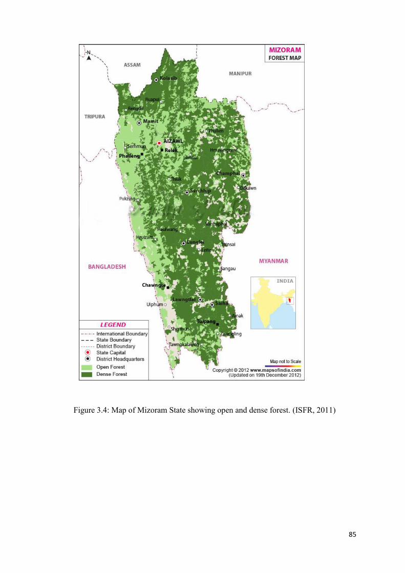
85
Figure 3.4: Map of Mizoram State showing open and dense forest. (ISFR, 2011)
86
Tropical Wet -Evergreen forests are found in the Southern and Western
parts of Mizoram. The common timber species found in these areas are Dipterocarpus
turbinatus, Artocarpus chaplasa, Terminalia myriocarpa, Duabanga sonneratoides,
Michelia champaca growing in association with undergrowth (Anon., 2003).
Tropical semi-evergreen covers the central bio-geographic zone and
the coverage is approximately 50 percent of the total geographic area. The common
tree species are Michelia champaca, Schima wallichi, Gmelina arborea, Catanopsis
tribuloidies etc. Bamboo species like Melocanna baccifera and Dendrocalamus
species and canes are abundant, especially in shady and low lying areas (Anon.,
2003).
The Montane sub-tropical pine forest occurs in the eastern fringes
bordering Myanmar and constitutes about 24 per cent of the total geographical area.
The common tree species are Pinus kesiya, Rhododendron arboretum, Quercus
serrata, Quercus griffithii, etc. (Anon., 2003).
3.5 Landuse Pattern and cropping system in Mizoram
Land within Mizoram, like some other states of North east, is in the
customary ownership of the communities. Village lands falling within the jurisdiction
of villages are controlled by the Village Council (s) and land distribution is done as
per the customary practice to the villagers for jhumming and other farming activities.
The landuse pattern of the state has been affected primarily by land capability as
determined by characteristics of micro and mini watersheds. Besides, several social
legal factors such as land tenure system etc. also affect the landuse pattern.

87
Agriculture is the main stay for about 60 per cent of the population of
Mizoram. Of the total area only 21 per cent is put on the paddy/ seasonal crops. As
high as 63 per cent of the total crops area is under jhum cultivation. The crops grown
in the jhum are mixed. The principal crop is paddy and others are maize, cucumber,
beans, arum, ginger, mustard, sesame, cotton etc. There is vast scope for cultivation of
tapioca, sugarcane, cotton, pulses and oil seeds in the State. Oil seeds crops like
sesame, mustard and soyabean are growing well in the state. Paddy occupies almost
50 per cent of the total cropped area and more than 88 per cent of the total area under
food grains (Anon., 2010).

88
CHAPTER IV
MATERIALS AND METHODS
4.1 Experimental Site
The experiment was conducted at Edenthar area which is at the outskirt
of Aizawl, the capital city of Mizoram State. The altitude is about 493m from MSL
with geographical coordinates of 23.754149° N and 92.714610°E. The hill slopes have
the soil orders of ultisols with sandy clay loam texture. The average annual rainfall in
this area is 2150 cm. The experiment was carried out in the month of March to July in
the year 2010. The surface soils are dark, highly leached and poor in bases, rich in
iron. pH and organic carbon content decrease and clay content increases with depth.
4.2 Experimental Design and treatments
The experiment was designed using Randomized Block Design (RBD)
with three replications. There was 12 sub-plots and each of the sub-plot was 4m x 3m
(12 sq.m) and each sub-plot is separated by 1 metre width buffer zone. Each
replication covered an area of 210 sq. metre.
Experimental Design : Randomized Block Design. (RBD)
No.of Replications : 3 (three)
Sub-Plot size : 4m x 3m ( 12 sq.m)
No.of Sub-Plots : 12 sub-plots under each replication (36 nos.)
Area of one plot size : 210 Sq.m
Area of total (3) plot size : 630 sq.m
Crop species : Zea mays L
Treatments : 12 treatments

89
4.3 Experimental Layout
R1: 4m
3M
R2 :
R3:
:
NS3F3S1F0 S3F0
1M
S2F2 S2F0
SS3F2
S3F1
S1F2 15M
S2F1S2F3
ES1F1S1F3
S1F1
S3F2
S1F2
S3F3
S3F1
S1F0
47M
S3F0
S2F1
S2F2
S2F0
S1F3
S2F3
S2F1
S3F0
S3F3
S1F0
S2F0
S1F1
S1F2
S3F2
15M
S3F1
S2F3
S1F3
S2F2
15M

90
Figure 4.1: Location of the experimental site at Edenthar showing the treatment plots
of the experimental block.
90
Figure 4.1: Location of the experimental site at Edenthar showing the treatment plots
of the experimental block.
90
Figure 4.1: Location of the experimental site at Edenthar showing the treatment plots
of the experimental block.
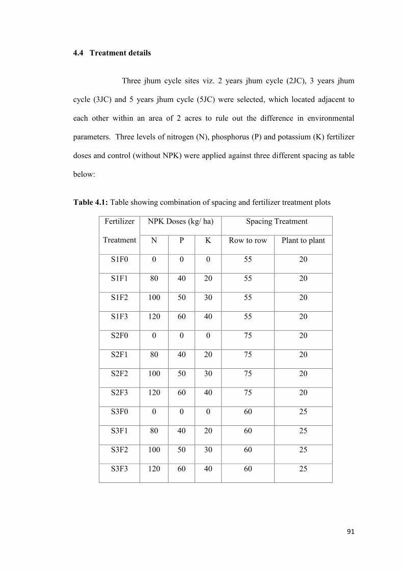
91
4.4 Treatment details
Three jhum cycle sites viz. 2 years jhum cycle (2JC), 3 years jhum
cycle (3JC) and 5 years jhum cycle (5JC) were selected, which located adjacent to
each other within an area of 2 acres to rule out the difference in environmental
parameters. Three levels of nitrogen (N), phosphorus (P) and potassium (K) fertilizer
doses and control (without NPK) were applied against three different spacing as table
below:
Table 4.1: Table showing combination of spacing and fertilizer treatment plots
Fertilizer
Treatment
NPK Doses (kg/ ha) Spacing Treatment
N P K Row to row Plant to plant
S1F0 0 0 0 55 20
S1F1 80 40 20 55 20
S1F2 100 50 30 55 20
S1F3 120 60 40 55 20
S2F0 0 0 0 75 20
S2F1 80 40 20 75 20
S2F2 100 50 30 75 20
S2F3 120 60 40 75 20
S3F0 0 0 0 60 25
S3F1 80 40 20 60 25
S3F2 100 50 30 60 25
S3F3 120 60 40 60 25

92
4.5 Application of NPK fertilizer
A mixture of Urea (N), Single Super Phosphate (P) and Muriate of
Potash (K) is applied in the field in three different doses such as 120, 60, 40 kg/ha;
100, 50, 30 kg/ ha; 80, 40 20 kg/ha respectively at two split doses in the field before
tillering and after sowing.
4.6 Details of collection of Data
4.6.1 Soil sample collection
Prior to land preparation soil samples were collected from 12 locations
in each replication from three jhum cycle sites by using spade from a depth of 0- 30
cm on one day before the start of the experiment . Soil samples were collected and
packed in the polythene bag. The three jhum plots were slashed and burnt before the
experiment. The soil samples were serially registered giving all the necessary
information mentioning the sample number, place of collection, depth of collection of
samples and site description.
4.6.2 Processing of soil samples
The soil samples were air dried and crushed and passed through sieves
of finer mesh size (Ghosh et al., 1983).
4.6.3 Determination of pH
The pH of the soil samples was measured by the method of soil to water ratio

93
of 1:2. Soil samples of 20 g was taken in a 100 ml beaker to which 40 ml of water was
added. The suspension was stirred at regular intervals for 30 minutes and the pH was
recorded with the help of pH meter.
4.6.4 Estimation of Organic Carbon
The method given by Walkley and Black (1934) was adopted to
estimate Organic Carbon. Soil samples were grounded and completely passed through
0.2mm sieve and 1.00g of it was kept at the bottom of a dry 500ml conical flask. Then
10ml of 1N K2Cr2O7 was pipetted in and swirled a little. The flask was kept on
asbestos sheet. Then 20 ml of H2SO4 (containing 1.25% Ag2SO4) was run in an
swirled again two or three times. The flask was allowed to stand for 30 minutes;
thereafter, 200ml of distilled water was added. Thereafter, 10ml of phosphoric acid or
0.5g Sodium fluoride and 1ml of diphenylamine indicator was added and titrated with
ferrous Ammonium Sulphate solution till the colour flashes from the blue violet to
green. Simulteneously, a blank was run without soil. The result was calculated by the
following method:
Organic Carbon (%) = 10(B-T) x 0.003 x 100
B Wt. of soil
(Where B= Volume (in ml) of ferrous ammonium sulphate solution required for blank
titration; & T= Volume of ferrous ammonium sulphate needed for soil sample).
4.6.5 Estimation of Nitrogen (N) content
The procedure for the analysis of Nitrogen content in the soil samples
was divided into three steps, viz. digestion, distillation and titration.

94
Digestion: 1gm of soil sample was taken in each of Kjeldahl flask for
digestion tube and 10ml Conc. Sulphuric Acid was added in each flask. Also, 3gms of
catalyst mixture (Kjeldahl catalyst) was added in each of digestion tube and the
balance without a soil sample was maintained. Temperature was set at 420oC and it
was digested for approximately 1hr till the sample became green colour. Then, the
digester was switched off and the flask was allowed to cool.
Distillation: Firstly, the conical flask was loaded (with 20ml of 40%
Boric Acid) in the receiver side whch will be pink colour as it contain 3 drops of
Bromo cresol green and Methyl red solution of 5 drops. Then, the digested sample
was loaded for distillation. Again, 40% of NaOH was added slowly in automode in
the order of 10ml each time till the colour changes from bluish green to brown
precipitation and the process time was set for 6 minutes for soil sample. After 6
minutes, the sample colour in a conical flask changed fro pink to green to green
colour which was the end point. The flask was then prepared for titration.
Titration: The distillated was titrated against 0.1N HCl. The titration
was stopped when the colour changed from green to pake pink.
% of Nitrogen = 14 x Titrant value x Normality of acid x 100
1000 x Sample wt.
4.6.6 Estimation of phosphorus
The methods developed by Olsen et al., (1954) and Dickman & Brays
(1940) was followed for the estimation of Phosphorus in the soil samples. 2.5g of the
soil sample was taken in 100ml conical flask and a little of Dargo G 60 or equivalent
grade of activated carbon (free of phosphorus) was added followed by 50ml of
95
Olsen’s reagent. A blank is run without soil. Then the flask were shaken for 30
minutes on a platform type shaker and the contents are filtered immediately through
dry filter paper (Whatman No. 1) into dry beakers or vials.
In the filtrate, phosphorus was estimated calorimetrically by Dickman
and Bray’s procedure (Dickman and Brays, 1940). 5ml of soil extract is pipette into a
25ml volumetric flask to which 5ml of the Dickman and Bray’s reagent was poured
in. The rock of the flask was washed down and the content was diluted to about 22ml.
Therefore, 1ml of the diluted stannous chloride solution was added and the volume
makes up to the mark level. The intensity of the blue colour was measured (using mµ
filter) just after 10 minutes and the concentration of phosphorus was determined from
the standard curve. With each sample a blank was maintained.
4.6.7 Estimation of Potassium
Available Potassium (K) incorporates both exchangeable and water
soluble forms of the nutrient present in the soil. The estimation of K of water soluble
forms was carried out with the help of Flame photometer as suggested by Ghost et al.,
(1983). 5gms of soil sample was shaken with 25ml of normal of Ammonium acetate
(pH 7) for 5 minutes and filtered immediately through a dry filter paper (Whatman
No. 1). First few ml of the filtrate was rejected. Potassium concentration in the extract
was determined in the flame photometer.

96
4.7 Biometrical observations
4.7.1 Growth parameters of maize
i) Plant height (cm): Plant height were recorded in situ at 15, 30, 45 and 60
Days After Sowing (DAS) by randomly selecting 10 plants from each plot
and heights were measured by linear scale from the ground level up to the
flag leaf. The mean values were computed and expressed in cm.
ii) Number of leaves per plant: The number of leaves of 10 tagged plants
from each plot were counted at different stages of 15, 30, 45 and 60 DAS
and the mean number of leaves per plant were recorded.
iii) Plant biomass (gm): The plant aboveground biomass was harvested at plant
maturity stage by cutting at the ground level. The plant material was cut into
manageable size and kept in hot air oven at 70oC until constant weight of
dryness was obtained. The dry plant material was then weighed using digital
weighing balance and expressed in gram (gm).
4.7.2 Yield parameters of maize
i) Number of cobs per plant: The number of cob per plant was recorded
from 10 plants which were randomly selected from each plot and the mean
number of cob per plant were recorded.
ii) Length of cobs: Ten cobs per plot were randomly selected at the time of
harvesting and the length of the cobs were measured and the mean cobs
length were computed and expressed in cm.
97
iii) Number of kernel’s row per cob: From the randomly selected 10 cobs
from each plot, the number of kernels row per cob were counted and the
mean number of row were recorded.
iv) Number of kernels per row: The number of kernels in a row from
randomly selected cobs from each plot were counted and the mean number
were computed.
v) Test weight (1000 grain weight): One thousand filled grains were counted
from the grain sample and their weight were recorded in grams.
vi) Grain yield: The grain yield of maize for each treatment was calculated by
using the formula,
Grain yield (kg/ ha.) = 1 ha. X Yield per plot (kg)
Net area of plot
viii) Harvest Index: The term “harvest index” is used to quantify the yield of a
crop species versus the total amount of biomass that has been produced. The
commercial yield can be grain, tuber or fruit. Harvest index can apply
equally well to the ratio of yield to total plant biomass (shoots plus roots) but
above-ground biomass is more common because root mass is so difficult to
obtain. The harvest index of the maize for each treatment was calculated by
using the formula,
Harvest index % = Economic yield (grains) x 100
Biological yield (Straw + grains

98
4.7.3 Statistical Analysis
The experimental data pertaining to each parameters were analyzed
statistically. ANOVA was performed with the help of SigmaStat 4.0 software and
Costat software.
.

99
Chapter – V
Results
Table 5.1 Monthly rainfall of 2010 showing the rainfall pattern during the
experimental period.
The rainfall pattern showed high rainfall during the experimental period from March
to August, 2010. As maize is a water demanding crop, the experiment was conducted
during the rainy seasons as kharif crop (Table 5.1). In Mizoram the slash and burning
of forest vegetation occurred during the February and mid of March. Sowing of seeds
is done mostly during end of March to May depending on the rainfall.
Table 5.2 Soil properties of 2JC, 3JC and 5JC before land preparation.
0.1 15.8
135197.7
308383.5
282.6
493.8405.7
246.3
15.2 49.2
0100200300400500600
Jan Feb Mar Apr May Jun Jul Aug Sep Oct Nov Dec
Rain
falll
(mm
)
Month
Jhum cycles pH OC(%)
P2O5(kg/ha)
K2O(kg/ha)
Total N(%)
Soil texture
2 JC 6.15 1.38 7.56 120 0.26 Sandy clay loam3 JC 6.18 1.67 9.32 145 0.32 Sandy clay loam5 JC 6.24 3.11 11.33 180 0.47 Sandy clay loam

100
5.2 Soil analysis
Soil properties of the three Jhum sites sampled before the land preparation for the
experiment (Table 1) showed soil pH ranging from 6.15 in 2 years jhum to 6.24 in 5
years jhum. Similar trend with lowest values in 2 years jhum and highest 5 years
jhum was also observed in other soil parameters ranging from 1.38 to 3.11 kg/ha in
soil OC content, 7.56 to 11.33 kg/ha in available phosphate, 120 to 180 kg/ha in
available potassium and 0.26 to 0.4 % in total nitrogen content (Table 5.2). Although
slightly higher value in pH and higher content of OC, available phosphate, available
potash and total nitrogen content occurred in longer jhum periods, all the soil in the
three jhum cycles represent poor nutrient content for annual crop plantation.
5.3 Effect of Fertilizer application on growth performance
5.3.1 Plant height at 15 days after sowing:
As mentioned earlier, seeds were sown on 24th March, 2010 during
which summer rain occurred. In response to the immediate rainfall after seed sowing,
sprouting was observed from four days after sowing (DAS) of seeds. Measurement of
plant height at 15 DAS showed significant variations among the fertilizer plots under
each spacing treatment (Figure 5.3.1 & Table 5.3.1). Increased in plant height with
increasing level of fertilizer application occurred in all the fertilizer plots of each
spacing. In 2JC, minimum height of 13.85±0.46cm occurred in F0 plot of S1 spacing
while maximum height of 18.38±0.28cm occurred in F3 plot of S3 spacing. In 3JC, in
all the 3 spacing, minimum height ranging from 14.43±0.53cm to 15.14±0.47cm
occurred in plots without fertilizer application where as maximum height ranging
from 18.54±0.33 cm to 18.88±0.23cm occurred in plots with highest fertilizer
application. In 5JC, the plant height of fertilizer plots under S2 spacing showed
highest range of 14.77±0.34 cm (S2F0) to 19.11±0.19cm (S2F3).

101
5.3.2 Plant height at 30 DAS
Plant height at 30 DAS showed significant increase from F0 to F3 plots
in S1 spacing in all the jhum cycles. Except in 2JC, the fertilizer plots under S2 and
S3 spacing showed lesser variations in plant height. Comparatively lower plant height
was observed among the different fertilizer plots under highest density spacing of S1
than that S2 and S3. The maximum height of 63.70±1.96cm (S1F3) in 3JC and
79.87±1.15cm (S1F3) in 5JC of the S1 spacing was comparable to the minimum
values of 63.46±1.96 cm (S3F0) in 3JC and 81.30±3.01cm (S3F0) in 5JC of S3
spacing (Figure 5.3.2 & Table 5.3.2).
Unlike 15 DAS, the plant height in 30 DAS showed marked variations
with high significant levels among the jhum cycles and the minimum values occurred
in plots without fertilizer application under highest density spacing in S1F0 ranging
from 43.16±1.95 cm in 2JC to 68.28±1.40cm in 5JC.
5.3.3 Plant height at 45 DAS
With the increase in growth duration, wider range in plant height
among the fertilizer plots in each of the three spacing was observed. The high increase
in plant height from the 30DAS to 45DAS indicated high growth rate of plants during
30 to 45 DAS, and comparative highly growth rate occurred in the fertilizer plots
under S1 spacing. Statistically significant variations were observed among the
fertilizer plots in under each of the three spacing (Figure 5.3.3 & Table 5.3.3). In 2JC,
under the S1, S2 and S3 spacing, the minimum height to the maximum height ranged
from 79.74±1.40 (S1F0) to 101.92±2.01cm (S1F3), 85.64±1.56 cm (S2F0) to
118.50±4.15 cm (S2F3) and, 83.55±3.36 cm (S3F0) to 122.42±6.62cm (S3F3) which
accounted for 27.81%, 38.36%, 46.52%, increase in plant height respectively.

102
Significant response to fertilizer treatment was observed in 3JC ranging from
89.60±3.32cm (S1F0) to 121.09±5.11cm (S1F3) under S1 spacing, 97.83±2.92cm
(S2F0) to 131.67±4.49cm (S2F3) under S2 spacing and, 106.73±2.98cm (S3F0) to
131.26±5.41cm (S3F3) under S3 spacing which accounted for the increase in 35.14%,
34.59%, 22.98% with fertilizer application in S1, S2 and S3 spacing respectively. In
5JC, less significant variation ranging from 142.34±3.56cm (S1F0) to 170.67±4.33
cm (S1F3) was observed in S1 spacing while higher significant difference ranging
from 159.81±3.50 cm (S2F0) to 184.26±3.14cm (S2F3) in S2 spacing and,
153.94±2.40cm (S3F0) to 181.31±3.44cm (S3F3) in S3 Spacing was recorded which
accounted for 19.90%, 15.29%, 17.77% increase from the minimum height.
The inter jhum comparison of each fertilizer plots showed highly significant
difference (P<0.001). In plot without fertilizer application (F0), the increase in plant
height from 2JC to 5JC ranged from 79.74±1.40cm to 142.34cm in S1, 85.64±1.56
cm to 159.81±3.50 cm in S2 and, 83.55±3.36cm to 153.94±2.40cm in S3.
5.3.4 Plant height at 60DAS
The height measurement at 60DAS showed high growth rate between
45 and 60DAS in 2JC and 3JC where around 100% increase in plant was observed. In
2JC, the significant difference in height ranged from 162.23±4.12cm (S1F0) to
184.63±5.14cm (S1F3) in S1 spacing; 185.61±3.38cm (S2F0) to 215.34±2.49cm
(S2F3) in S2 spacing and, 188.32±1.48cm (S3F0) to 212.72±3.29cm (S3F3) in S3
spacing which accounted for %%% increase in height from their respective minimum
height. 3JC also showed similar trend with minimum and maximum plant height
ranging from 165.38±2.10cm in (S1F0) to 212.54±1.36cm (S1F3) in S1 spacing,
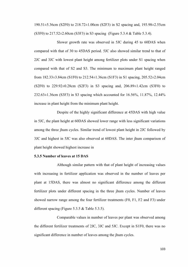
103
190.51±5.36cm (S2F0) to 218.72±1.00cm (S2F3) in S2 spacing and, 193.98±2.55cm
(S3F0) to 217.52±2.60cm (S3F3) in S3 spacing (Figure 5.3.4 & Table 5.3.4).
Slower growth rate was observed in 5JC during 45 to 60DAS when
compared with that of 30 to 45DAS period. 5JC also showed similar trend to that of
2JC and 3JC with lowest plant height among fertilizer plots under S1 spacing when
compared with that of S2 and S3. The minimum to maximum plant height ranged
from 182.33±3.84cm (S1F0) to 212.54±1.36cm (S1F3) in S1 spacing, 205.52±2.04cm
(S2F0) to 229.92±0.28cm (S2F3) in S3 spacing and, 206.89±1.42cm (S3F0) to
232.63±1.36cm (S3F3) in S3 spacing which accounted for 16.56%, 11.87%, 12.44%
increase in plant height from the minimum plant height.
Despite of the highly significant difference at 45DAS with high value
in 5JC, the plant height at 60DAS showed lower range with less significant variations
among the three jhum cycles. Similar trend of lowest plant height in 2JC followed by
3JC and highest in 5JC was also observed at 60DAS. The inter jhum comparison of
plant height showed highest increase in
5.3.5 Number of leaves at 15 DAS
Although similar pattern with that of plant height of increasing values
with increasing in fertilizer application was observed in the number of leaves per
plant at 15DAS, there was almost no significant difference among the different
fertilizer plots under different spacing in the three jhum cycles. Number of leaves
showed narrow range among the four fertilizer treatments (F0, F1, F2 and F3) under
different spacing (Figure 5.3.5 & Table 5.3.5).
Comparable values in number of leaves per plant was observed among
the different fertilizer treatments of 2JC, 3JC and 5JC. Except in S1F0, there was no
significant difference in number of leaves among the jhum cycles.
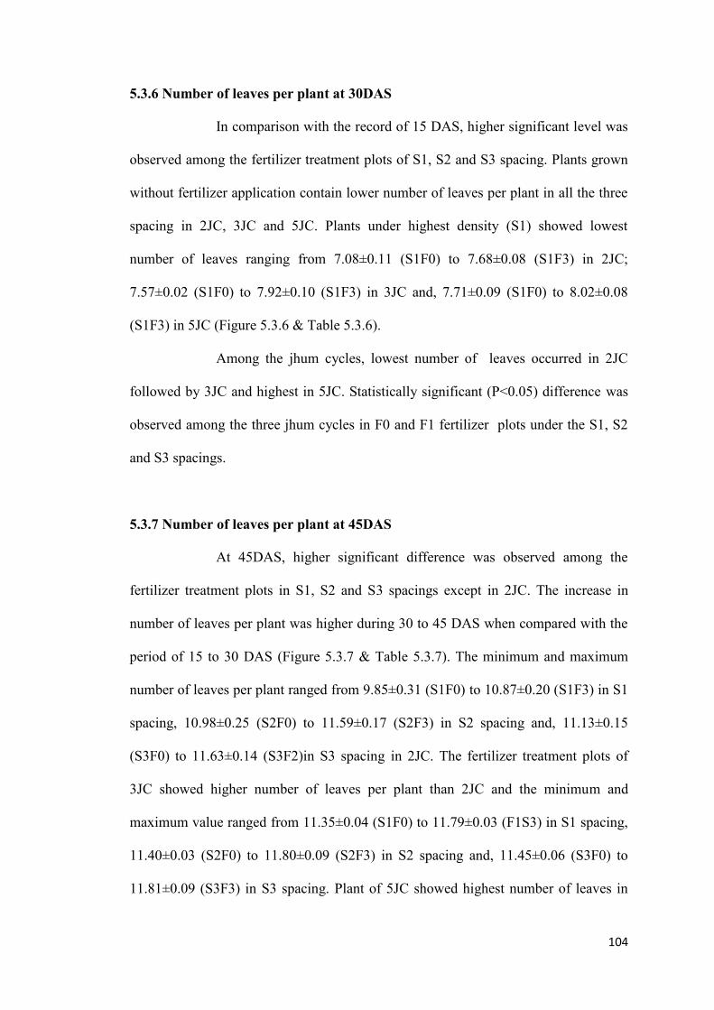
104
5.3.6 Number of leaves per plant at 30DAS
In comparison with the record of 15 DAS, higher significant level was
observed among the fertilizer treatment plots of S1, S2 and S3 spacing. Plants grown
without fertilizer application contain lower number of leaves per plant in all the three
spacing in 2JC, 3JC and 5JC. Plants under highest density (S1) showed lowest
number of leaves ranging from 7.08±0.11 (S1F0) to 7.68±0.08 (S1F3) in 2JC;
7.57±0.02 (S1F0) to 7.92±0.10 (S1F3) in 3JC and, 7.71±0.09 (S1F0) to 8.02±0.08
(S1F3) in 5JC (Figure 5.3.6 & Table 5.3.6).
Among the jhum cycles, lowest number of leaves occurred in 2JC
followed by 3JC and highest in 5JC. Statistically significant (P<0.05) difference was
observed among the three jhum cycles in F0 and F1 fertilizer plots under the S1, S2
and S3 spacings.
5.3.7 Number of leaves per plant at 45DAS
At 45DAS, higher significant difference was observed among the
fertilizer treatment plots in S1, S2 and S3 spacings except in 2JC. The increase in
number of leaves per plant was higher during 30 to 45 DAS when compared with the
period of 15 to 30 DAS (Figure 5.3.7 & Table 5.3.7). The minimum and maximum
number of leaves per plant ranged from 9.85±0.31 (S1F0) to 10.87±0.20 (S1F3) in S1
spacing, 10.98±0.25 (S2F0) to 11.59±0.17 (S2F3) in S2 spacing and, 11.13±0.15
(S3F0) to 11.63±0.14 (S3F2)in S3 spacing in 2JC. The fertilizer treatment plots of
3JC showed higher number of leaves per plant than 2JC and the minimum and
maximum value ranged from 11.35±0.04 (S1F0) to 11.79±0.03 (F1S3) in S1 spacing,
11.40±0.03 (S2F0) to 11.80±0.09 (S2F3) in S2 spacing and, 11.45±0.06 (S3F0) to
11.81±0.09 (S3F3) in S3 spacing. Plant of 5JC showed highest number of leaves in

105
each fertilizer treatment plots ranging from 11.79±0.04 (S1F0) to 12.22±0.02 (S1F3)
in S1, 11.84±0.01 (S2F0) to 12.25±0.03 (S2F3) and, 11.82±0.05 (S3F0) to
12.21±0.04 (S3F3) in S3 spacing.
5.3.8 Number of leaves per plant at 60DAS
In 2JC, significant difference in number of leaves per plant ranging
from 10.59±0.17 (S1F0) to 11.50±0.09 (S1F3) in S1 spacing, 11.98±0.05 (S2F0) to
12.56±0.02 (S2F3) in S2 spacing and, 12.09±0.06 (S3F0) to 12.55±0.06 (S3F3) in S3
spacing which accounted for 8.50%, 4.48% and 3.80% increase from the minimum
value respectively (Figure 5.3.8 & Table 5.3.8). Surprisingly reduction in number of
leaves per plant from that of 45DAS was observed in most of the fertilizer plots in S1
of 3JC and 5JC. In 3JC, the minimum and maximum values ranged from 10.49±0.36
(S1F0) to 11.17±0.05 (S1F3) in S1, 12.06±0.15 (S2F0) to 12.78±0.34 (S2F3) in S2
spacing and, 12.18±0.11 (S3F0) to 12.99±0.25 (S3F3) in S3 spacing which accounted
for 6.48%, 5.97%, 6.65% increase from the minimum values. In 5JC, the minimum
and maximum values ranged from 10.87±0.34 (S1F0) to 12.34±0.14 (S1F3) in S1
spacing, 12.48±0.28 (S2F0) to 13.68±0.07 (S2F3) in S2 cycle and, 12.27±0.54 (S3F0)
to 13.66±0.05 (S3F3) in S3 spacing which accounted for increase in 13.52%, 9.61%,
11.32% for the minimum values respectively.
5.3.9 Biomass at harvest
Ten plants per replication was harvested at maturity stage at 23rd &
24th July, 2010 for the determination of biomass. The plant dry biomass at maturity
harvest showed significant variations among the different fertilizer plots of S1, S2 and
S3 spacing. Among three spacing, the fertilizer plots of S1 spacing showed much

106
lesser plant biomass ranging from 264.50±17.37gm (S1F0) to 319.50± 13.12 gm
(S1F3) in S1 spacing, 318.50±14.40 gm (S2F0) to 371.50±6.08 gm (S2F3) in S2
spacing and, 316.50±3.97 gm (S3F0) to 374.20±4.09 gm (S3F3) in S3 spacing. Slight
increase in dry biomass per plant from 2JC was observed in 3JC (except S2F0) with
minimum to maximum plant biomass ranging from 267.77±4.91 gm (S1F0) to
322.38±6.39 gm (S1F3) in S1 spacing, 308.55±3.87 gm (S2F0) to 376.03±5.67 gm
(S2F3) in S2 spacing and, 319.66±3.01 gm (S3F0) to 377.08±2.28 gm (S3F3) in S3
spacing. Highest dry biomass per plant was observed in 5JC which ranged from
292.60±4.50 gm (S1F0) to 327.13±5.96 gm (S1F3) in S1 spacing, 335.80±2.75 gm
(S2F0) to 386.11±1.79 gm (S2F3) in S2 spacing and, 337.72±2.78 gm (S3F0) to
390.93±4.39 gm (S3F3) in S3 spacing (Figure 5.3.9 & Table 5.3.9).
The percentage increase in plant biomass from the plot without
fertilizer application to the highest fertilizer application in S1, S2 and S3 spacing were
20.79%, 16.64% and 18.23%, in 2JC, 20.40%, 21.87% and 17.96% in 3JC and,
11.80%, 14.98% and 15.75% in 5JC.
Among the jhum cycle, lowest biomass production occurred in 2JC
follow by 3JC and highest in 5JC. Low level of significant difference was observed in
each fertilizer plots of S1 spacing. In S2 spacing, significant difference among jhum
cycles was observed in S2F1 and S2F3. Each fertilizer plots of S3 spacing showed
significant difference (P<0.05 to P>0.001). From the all the fertilizer treatments of the
three jhum cycles, the lowest biomass per plant of 264.50±7.37gm (S1F0) of 2JC to
390.93±4.29gm (S3F3) of 5JC accounted for 47.79% increased in plant biomass.
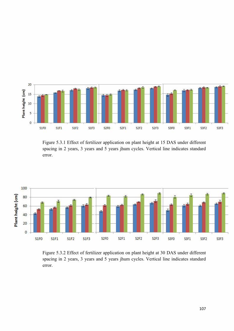
107
Figure 5.3.1 Effect of fertilizer application on plant height at 15 DAS under differentspacing in 2 years, 3 years and 5 years jhum cycles. Vertical line indicates standarderror.
Figure 5.3.2 Effect of fertilizer application on plant height at 30 DAS under differentspacing in 2 years, 3 years and 5 years jhum cycles. Vertical line indicates standarderror.
108
Table5.3.1: Plant height at 15 days after sowing (DAS) under different spacing andfertilizer application levels in 2, 3 and 5 years jhum cycles. Mean ±SEM.
* = P<0.05, ** = P<0.01, *** = P<0.001
Table5.3.2: Plant height at 30 days after sowing (DAS) under different spacing andfertilizer application levels in 2, 3 and 5 years jhum cycles. Mean ±SEM.
* = P<0.05, ** = P<0.01, *** = P<0.001.
S1F0 S1F1 S1F2 S1F3LSD(0.05) S2F0 S2F1 S2F2 S2F3
LSD(0.05) S3F0 S3F1 S3F2 S3F3
LSD(0.05)
2JC43.16±1.95
52.88±1.96
56.60±1.70
60.66±2.71
**7.77
48.18±1.90
59.57±2.32
63.62±1.34
66.94±1.81
***7.37
50.87±2.94
61.59±2.94
61.30±1.66
65.69±1.73
*10.71
3JC52.72±1.57
56.83±1.36
61.27±1.87
63.70±1.96
**6.87
61.76±2.21
62.53±1.60
69.63±0.51
71.41±3.18
*2.37
63.46±1.96
64.90±2.43
68.67±1.24
70.44±3.39
ns
5JC68.28±1.40
71.14±2.70
74.67±1.38
79.87±1.15
**6.33
83.79±1.54
82.32±2.09
87.18±1.35
89.38±1.57
ns 81.30±3.01
84.83±3.27
87.69±1.83
89.56±1.57
ns
LSD(0.05)
***9.56
**14.31
***13.4
**16.16
***13.57
***19.78
***6.01
**17.97
***12.59
**19.92
***7.36
***19.12
S1F0 S1F1 S1F2 S1F3LSD(0.05) S2F0 S2F1 S2F2 S2F3
LSD(0.05) S3F0 S3F1 S3F2 S3F3
LSD(0.05)
2JC13.85±0.46
15.80±0.11
17.16±0.36
18.13±0.55
***1.26
14.42±0.48
16.78±0.47
17.30±0.34
18.10±0.23
**2.35
14.47±0.67
16.69±0.59
17.96±0.29
18.38±0.28
**1.69
3JC14.43±0.53
16.91±0.16
17.98±0.34
18.54±0.33
***1.63
14.37±0.61
17.19±0.31
18.19±0.29
18.88±0.23
***3.03
15.14±0.47
16.90±0.34
18.26±0.46
18.86±0.44
**1.76
5JC14.90±0.11
16.72±0.54
17.44±0.42
18.62±0.29
***1.82
14.77±0.34
17.06±0.40
18.52±0.51
19.11±0.19
***1.45
16.86±0.17
17.11±0.33
18.13±0.13
18.96±0.13
***0.83
LSD(0.05) ns ns ns ns ns ns Ns
*0.78
*1.72 ns ns ns

109
Figure 5.3.3 Effect of fertilizer application on plant height at 45 DAS under differentspacing in 2 years, 3 years and 5 years jhum cycles. Vertical line indicates standarderror.
Figure 5.3.4 Effect of fertilizer application on plant height at 60DAS under differentspacing in 2 years, 3 years and 5 years jhum cycles. Vertical line indicates standarderror.

110
Table 5.3.3 : Plant height at 45 days after sowing (DAS) under different spacing andfertilizer application levels in 2, 3 and 5 years jhum cycles. Mean ±SEM.
* = P<0.05, ** = P<0.01, *** = P<0.001.
Table 5.3.4: Plant height at 60 days after sowing (DAS) under different spacing andfertilizer application levels in 2, 3 and 5 years jhum cycles. Mean ±SEM.
* = P<0.05, ** = P<0.01, *** = P<0.001.
S1F0 S1F1 S1F2 S1F3LSD(0.05) S2F0 S2F1 S2F2 S2F3
LSD(0.05) S3F0 S3F1 S3F2 S3F3
LSD(0.05)
2JC162.23
±4.12169.03
±3.84177.50
±5.02184.63
±5.14*15.26
185.61±3.38
195.74±3.36
207.87±2.62
215.34±2.49
***10.13
188.32±1.48
197.45±4.72
206.25±1.92
212.72±3.29
**15.26
3JC165.38
±2.10177.44
±5.60186.50
±4.55196.14
±5.32**18.7
190.51±5.36
200.58±1.64
210.98±2.39
218.72±1.00
***10.40
193.98±2.55
202.05±2.01
209.45±4.19
217.52±2.60
**15.47
5JC183.33
±3.84194.88
±3.47201.41
±4.70212.54
±1.36**17.66
205.52±2.04
212.32±2.92
217.45±2.10
229.92±0.28
***6.80
206.89±1.42
211.03±1.84
217.83±2.27
232.63±1.36
***6.80
LSD(0.05)
**17.95
*17.43
*23.91
*16.39
*15
*11.73 ns
**11.2
**12.91 ns ns
**15.11
S1F0 S1F1 S1F2 S1F3LSD(0.05) S2F0 S2F1 S2F2 S2F3
LSD(0.05) S3F0 S3F1 S3F2 S3F3
LSD(0.05)
2JC79.74±1.40
89.46±1.88
97.52±5.89
101.92±2.01
**12.46
85.64±1.56
100.03±3.37
112.10±4.15
118.50±4.15
***12.06
83.55±3.36
98.28±2.67
115.34±3.51
122.42±6.62
***14.72
3JC89.60±3.32
101.63±1.61
109.35±1.43
121.09±5.11
***11.73
97.83±2.92
103.21±2.47
118.93±5.17
131.67±4.49
**15.72
106.73±2.98
111.11±3.35
122.84±2.54
131.26±5.41
**16.11
5JC142.34±3.56
157.08±5.69
163.85±3.57
170.67±4.33
*14.74
159.81±3.50
166.56±2.89
171.34±4.21
184.26±3.14
**11.53
153.94±2.40
168.37±4.06
175.33±3.48
181.31±3.44
**12.94
LSD(0.05)
***52.74
***55.44
***54.49
***19.16
***12.18
***63.35
***52.4
***52.58
***23.18
***12.83
***52.49
***50.05

111
Figure 5.3.5 Effect of fertilizer application on number of leaves per plant at 15 DASunder different spacing in 2 years, 3 years and 5 years jhum cycles. Vertical lineindicates standard error.
Figure 5.3.6 Effect of fertilizer application on plant height at 30 DAS under differentspacing in 2 years, 3 years and 5 years jhum cycles. Vertical line indicates standarderror.
112
Table 5.3.5 : No. of Leaves at 15 days after sowing (DAS) under different spacing andfertilizer application levels in 2, 3 and 5 years jhum cycles. Mean ±SEM.
* = P<0.05, ** = P<0.01, *** = P<0.001.
Table 5.3.6: No. of Leaves at 30 days after sowing (DAS) under different spacing andfertilizer application levels in 2, 3 and 5 years jhum cycles. Mean ±SEM.
* = P<0.05, ** = P<0.01, *** = P<0.001.
S1F0 S1F1 S1F2 S1F3LSD(0.05) S2F0 S2F1 S2F2 S2F3
LSD(0.05) S3F0 S3F1 S3F2 S3F3
LSD(0.05)
2JC5.11
±0.035.54
±0.105.56
±0.1115.80
±0.06**0.43
5.29±0.08
5.58±0.10
5.63±0.12
5.76±0.10 NS
5.44±0.10
5.65±0.09
5.66±0.11
5.70±0.10 NS
3JC5.15
±0.085.55
±0.0865.61
±0.095.83
±0.034**0.28
5.23±0.16
5.59±0.10
5.67±0.04
5.84±0.03
*2.45
5.45±0.10
5.62±0.06
5.69±0.07
5.86±0.04
*0.41
5JC5.47
±0.065.59
±0.095.65
±0.105.82
±0.034 NS5.53
±0.115.61
±0.055.68
±0.075.84
±0.03 NS5.58
±0.095.63
±0.085.70
±0.075.85
±0.02 NSLSD(0.05)
*0.32 ns ns ns ns ns ns ns ns ns ns ns
S1F0 S1F1 S1F2 S1F3LSD(0.05) S2F0 S2F1 S2F2 S2F3
LSD(0.05) S3F0 S3F1 S3F2 S3F3
LSD(0.05)
2JC7.08
±0.117.60
±0.047.65
±0.087.68
±0.08**0.52
7.13±0.04
7.65±0.06
7.64±0.07
7.71±0.10
**0.51
7.14±0.20
7.67±0.07
7.67±0.08
7.69±0.08
*0.53
3JC7.57
±0.027.69
±0.047.86
±0.097.92
±0.10*0.29
7.64±0.02
7.74±0.03
7.88±0.09
7.94±0.10 ns
7.63±0.02
7.77±0.03
7.90±0.09
7.94±0.10 ns
5JC7.71
±0.097.82
±0.047.91
±0.078.02
±0.08 ns7.76
±0.067.87
±0.027.96
±0.078.03
±0.06*0.20
7.77±0.05
7.89±0.00
7.99±0.07
8.05±0.08
*0.21
LSD(0.05)
**0.48
*0.21 ns ns
***0.5
*0.21 ns ns
*0.49
*0.22 ns ns

113
Figure 5.3.7 Effect of fertilizer application on number of leaves per plant at 45 DASunder different spacing in 2 years, 3 years and 5 years jhum cycles. Vertical lineindicates standard error.
Figure 5.3.8 Effect of fertilizer application on number of leaves per plant at 60 DASunder different spacing in 2 years, 3 years and 5 years jhum cycles. Vertical lineindicates standard error.
114
Table 5.3.7: No. of Leaves at 45 days after sowing (DAS) under different spacing andfertilizer application levels in 2, 3 and 5 years jhum cycles. Mean ±SEM
* = P<0.05, ** = P<0.01, *** = P<0.001.
Table 5.3.8: No. of Leaves at 60 days after sowing (DAS) under different spacing andfertilizer application levels in 2, 3 and 5 years jhum cycles. Mean ±SEM
* = P<0.05, ** = P<0.01, *** = P<0.001
S1F0 S1F1 S1F2 S1F3LSD(0.05) S2F0 S2F1 S2F2 S2F3
LSD(0.05) S3F0 S3F1 S3F2 S3F3
LSD(0.05)
2JC9.85
±0.3110.13±0.36
10.39±0.07
10.87±0.20 ns
10.98±0.25
11.48±0.15
11.53±0.14
11.59±0.17 ns
11.13±0.15
11.50±0.05
11.63±0.14
11.61±0.03
*0.37
3JC11.35±0.04
11.48±0.09
11.71±0.01
11.79±0.03
**0.23
11.40±0.03
11.57±0.05
11.74±0.02
11.80±0.09
**0.22
11.45±0.06
11.68±0.01
11.78±0.03
11.81±0.09
*0.22
5JC11.79±0.04
11.89±0.02
12.06±0.07
12.22±0.02
***0.15
11.84±0.01
11.92±0.02
12.10±0.10
12.25±0.03
**0.18
11.83±0.05
12.01±0.06
12.11±0.08
12.21±0.04
**0.20
LSD(0.05)
***1.49
**1.34
***0.35
***0.42
*0.86
*0.34
*0.36
*0.44
**0.37
***0.18
*0.47
**0.4
S1F0 S1F1 S1F2 S1F3LSD(0.05) S2F0 S2F1 S2F2 S2F3
LSD(0.05) S3F0 S3F1 S3F2 S3F3
LSD(0.05)
2JC10.59±0.17
10.71±0.28
11.25±0.07
11.50±0.09
*0.65
11.98±0.05
12.35±0.05
12.34±0.06
12.56±0.02
***0.21
12.09±0.06
12.34±0.02
12.41±0.04
12.55±0.06
**0.21
3JC10.49±0.36
10.69±0.32
10.97±0.24
11.17±0.05 ns
12.06±0.15
12.44±0.30
12.54±0.37
12.78±0.34 ns
12.18±0.11
12.45±0.33
12.58±0.27
12.99±0.25 ns
5JC10.87±0.34
11.32±0.07
11.98±0.17
12.34±0.14
**1.02
12.48±0.28
12.75±0.31
13.24±0.15
13.68±0.07
*0.76
12.27±0.54
12.80±0.30
13.25±0.18
13.66±0.05 ns
LSD(0.05) ns ns
*0.73
***0.84 ns ns ns
*0.9 ns ns
*0.67
**0.67
115
Figure 5.3.9 Effect of fertilizer application on number biomass production at maturityharvest under different spacing in 2 years, 3 years and 5 years jhum cycles. Verticalline indicates standard error.
Table 5.3.9: Biomass at maturity harvest under different spacing and fertilizerapplication levels in 2, 3 and 5 years jhum cycles. Mean ±SEM
* = P<0.05, ** = P<0.01, *** = P<0.001
S1F0 S1F1 S1F2 S1F3LSD(0.05) S2F0 S2F1 S2F2 S2F3
LSD(0.05) S3F0 S3F1 S3F2 S3F3
LSD(0.05)
2JC162.23
±4.12169.03
±3.84177.50
±5.02184.63
±5.14*15.26
185.61±3.38
195.74±3.36
207.87±2.62
215.34±2.49
***10.13
188.32±1.48
197.45±4.72
206.25±1.92
212.72±3.29
**15.26
3JC165.38
±2.10177.44
±5.60186.50
±4.55196.14
±5.32**18.7
190.51±5.36
200.58±1.64
210.98±2.39
218.72±1.00
***10.40
193.98±2.55
202.05±2.01
209.45±4.19
217.52±2.60
**15.47
5JC183.33
±3.84194.88
±3.47201.41
±4.70212.54
±1.36**17.66
205.52±2.04
212.32±2.92
217.45±2.10
229.92±0.28
***6.80
206.89±1.42
211.03±1.84
217.83±2.27
232.63±1.36
***6.80
LSD(0.05)
**17.95
*17.43
*23.91
*16.39
*15
*11.73 ns
**11.2
**12.91 ns ns
**15.11

116
5.4 Effect of fertilizer application on yield parameters
10 plants per replication plot was harvested on 23rd&24th July, 2010 for
the determination of yield parameters Number of cobs per plant was counted and all
the plants irrespective of difference levels of fertilizer application and jhum cycles
produce only one harvestable cob, and the second cob, if produced, was under-
developed and had no commercial value. So, only the first cob was considered in the
yield parameters.
5.4.1 Length of Cob
The plants grown under different fertilizer treatment showed marked
significant difference in S1, S2 and S3 spacing of 2JC and 3JC where as in 5JC,
significant difference was observed only in fertilizer plots under S1 spacing. In 2JC,
the minimum value was observed in F0 plot in S1, S2 and S3 spacing ranging from
14.70±0.17 cm (S1) to 17.50 cm (S3), and the maximum value in F3 plots ranged
from 17.31±0.14 cm (S1) to 19.10±0.31 cm (S3) (Figure 5.4.1 & Table 5.4.1). In 3JC,
the minimum values among S1, S2 and S3 ranged from 16.00±0.40 cm (S1F0) to
18.94±0.18 cm (S2F0) and the maximum values ranged from 18.87±0.18 cm (S1F3)
to 20.62±0.23 cm (S2F3). 5JC showed highest LoC with minimum values of
17.73±0.38 cm (S1F0), 20.66±0.12 cm (S2F0) and 20.65±0.16 cm (S3F0), and
maximum values of 20.16±0.18 cm (S1F0), 22.08±0.31 cm (S2F3) and 22.08±0.39
cm (S3F3).
Highly significant (P<0.01) difference was observed in each fertilizer
treatment plots among the jhum cycles. In S1 spacing, the maximum value of
17.31±0.14 cm (S1F2) in 2JC was comparable with the minimum value of
17.73±0.38 cm (S1F0) in 5JC. Likewise, the maximum value in LoC under high
117
fertilizer application plots of S2 and S3 of 2JC was comparable and slightly lower
than the corresponding minimum values of 5JC.
5.4.2 Kernel row per cob
Although increasing in kernel rows per cob with increasing fertilizer
application was observed in S1, S2 and S3 spacings, statistically significant difference
among the fertilizer treatment plots was observed only in S1 and S2 spacings of 2JC
(Figure 5.4.2 & Table 5.4.2). The maximum Kernel row per cob of 11.05±0.23 of
2JC, 11.45±0.12 of 3JC and 11.99±0.11 of 5JC in S1 spacing was lower than
minimum values of 11.61±0.22 (S2) and 11.74±0.18 (S3) of 2JC, 11.99±0.08 (S2)
and 12.19±0.15 (S3) of 3JC and, 12.63±0.09 (S2) and 12.71 (S3) of 5JC respectively.
Among the three jhum cycles, the difference in kernel row per cob was
statistically significant (P<0.05) in each of the fertilizer treatments with lowest
number in 2JC and increasing with longer jhum cycles.
5.4.3 Number of kernels per row
The number of kernels per row showed statistically significant
(P<0.05) different among the plants grown under different levels of fertilizer
application in all the three jhum cycles except in S2 spacing of 2JC. Evidently lower
number of kernels in each kernel row was observed in the fertilizer plots of S1
spacing when compared with their corresponding plots in S2 and S3 spacings in all
the three jhum cycles (Figure 5.4.3 &Table 5.4.3). Similar to the kernel row per cob,
the maximum number of kernels per row of 27.75±0.18 in 2JC, 30.90±0.10 in 3JC
and 32.90±0.29 in 5JC was lower than that of the minimum values of S2 spacing
(31.63±0.17, 35.01±0.33 and 36.67±0.19 in 2JC, 3JC and 5JC respectively) and S3
spacing (31.42±0.10, 34.51±0.11 and 36.70±0.38 in 2JC, 3JC and 5JC respectively).
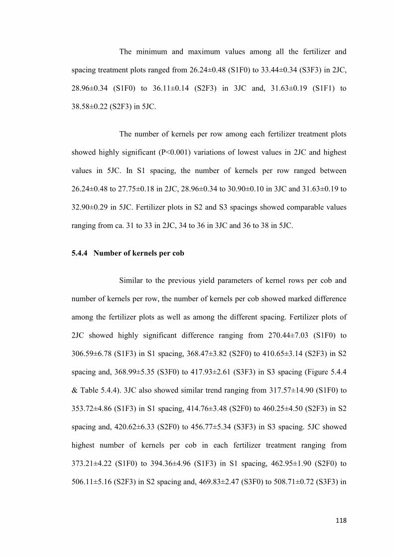
118
The minimum and maximum values among all the fertilizer and
spacing treatment plots ranged from 26.24±0.48 (S1F0) to 33.44±0.34 (S3F3) in 2JC,
28.96±0.34 (S1F0) to 36.11±0.14 (S2F3) in 3JC and, 31.63±0.19 (S1F1) to
38.58±0.22 (S2F3) in 5JC.
The number of kernels per row among each fertilizer treatment plots
showed highly significant (P<0.001) variations of lowest values in 2JC and highest
values in 5JC. In S1 spacing, the number of kernels per row ranged between
26.24±0.48 to 27.75±0.18 in 2JC, 28.96±0.34 to 30.90±0.10 in 3JC and 31.63±0.19 to
32.90±0.29 in 5JC. Fertilizer plots in S2 and S3 spacings showed comparable values
ranging from ca. 31 to 33 in 2JC, 34 to 36 in 3JC and 36 to 38 in 5JC.
5.4.4 Number of kernels per cob
Similar to the previous yield parameters of kernel rows per cob and
number of kernels per row, the number of kernels per cob showed marked difference
among the fertilizer plots as well as among the different spacing. Fertilizer plots of
2JC showed highly significant difference ranging from 270.44±7.03 (S1F0) to
306.59±6.78 (S1F3) in S1 spacing, 368.47±3.82 (S2F0) to 410.65±3.14 (S2F3) in S2
spacing and, 368.99±5.35 (S3F0) to 417.93±2.61 (S3F3) in S3 spacing (Figure 5.4.4
& Table 5.4.4). 3JC also showed similar trend ranging from 317.57±14.90 (S1F0) to
353.72±4.86 (S1F3) in S1 spacing, 414.76±3.48 (S2F0) to 460.25±4.50 (S2F3) in S2
spacing and, 420.62±6.33 (S2F0) to 456.77±5.34 (S3F3) in S3 spacing. 5JC showed
highest number of kernels per cob in each fertilizer treatment ranging from
373.21±4.22 (S1F0) to 394.36±4.96 (S1F3) in S1 spacing, 462.95±1.90 (S2F0) to
506.11±5.16 (S2F3) in S2 spacing and, 469.83±2.47 (S3F0) to 508.71±0.72 (S3F3) in
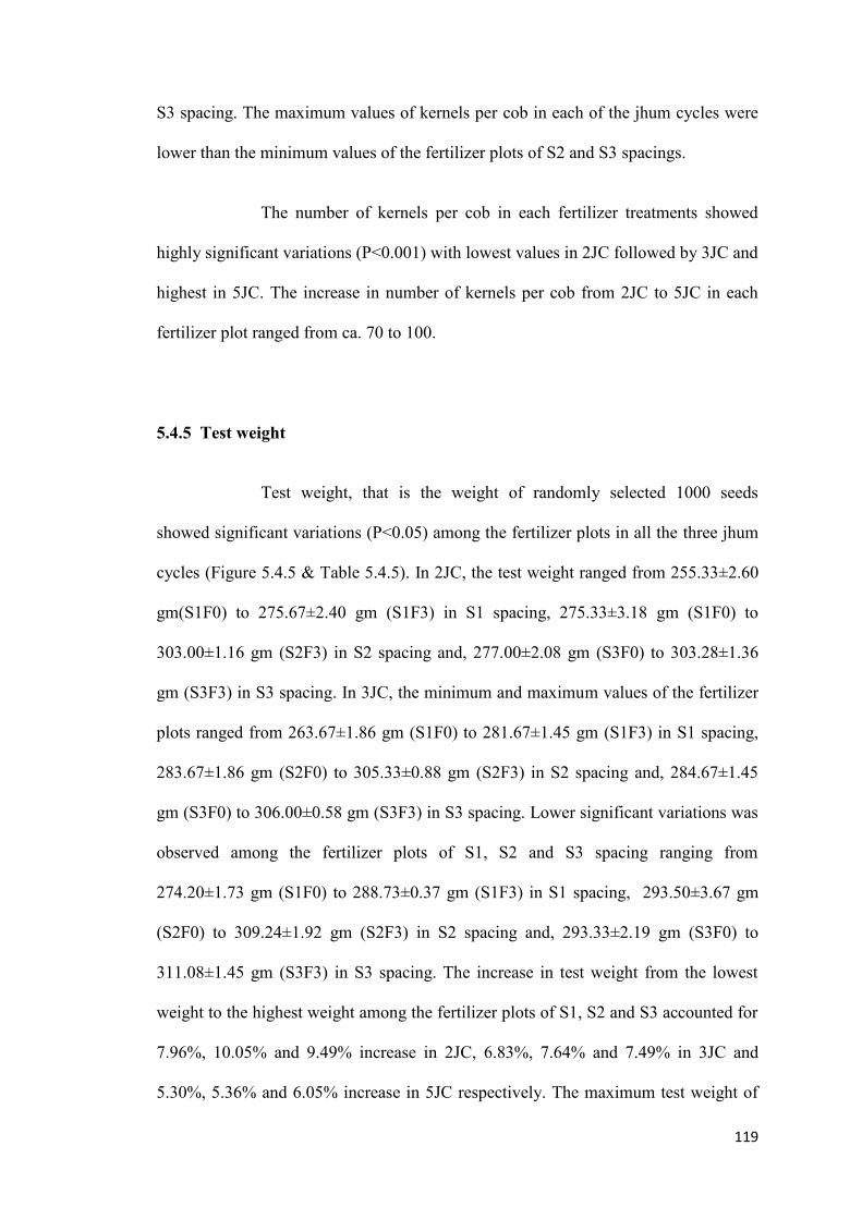
119
S3 spacing. The maximum values of kernels per cob in each of the jhum cycles were
lower than the minimum values of the fertilizer plots of S2 and S3 spacings.
The number of kernels per cob in each fertilizer treatments showed
highly significant variations (P<0.001) with lowest values in 2JC followed by 3JC and
highest in 5JC. The increase in number of kernels per cob from 2JC to 5JC in each
fertilizer plot ranged from ca. 70 to 100.
5.4.5 Test weight
Test weight, that is the weight of randomly selected 1000 seeds
showed significant variations (P<0.05) among the fertilizer plots in all the three jhum
cycles (Figure 5.4.5 & Table 5.4.5). In 2JC, the test weight ranged from 255.33±2.60
gm(S1F0) to 275.67±2.40 gm (S1F3) in S1 spacing, 275.33±3.18 gm (S1F0) to
303.00±1.16 gm (S2F3) in S2 spacing and, 277.00±2.08 gm (S3F0) to 303.28±1.36
gm (S3F3) in S3 spacing. In 3JC, the minimum and maximum values of the fertilizer
plots ranged from 263.67±1.86 gm (S1F0) to 281.67±1.45 gm (S1F3) in S1 spacing,
283.67±1.86 gm (S2F0) to 305.33±0.88 gm (S2F3) in S2 spacing and, 284.67±1.45
gm (S3F0) to 306.00±0.58 gm (S3F3) in S3 spacing. Lower significant variations was
observed among the fertilizer plots of S1, S2 and S3 spacing ranging from
274.20±1.73 gm (S1F0) to 288.73±0.37 gm (S1F3) in S1 spacing, 293.50±3.67 gm
(S2F0) to 309.24±1.92 gm (S2F3) in S2 spacing and, 293.33±2.19 gm (S3F0) to
311.08±1.45 gm (S3F3) in S3 spacing. The increase in test weight from the lowest
weight to the highest weight among the fertilizer plots of S1, S2 and S3 accounted for
7.96%, 10.05% and 9.49% increase in 2JC, 6.83%, 7.64% and 7.49% in 3JC and
5.30%, 5.36% and 6.05% increase in 5JC respectively. The maximum test weight of

120
S1F3 plots in S1 was comparable with the lowest weight of the plots without fertilizer
input (F0) in S2 and S3.
The test weight in each fertilizer plots among the jhum cycles showed
significant variations S1F0, S1F1, S1F3, S2F0, S2F2, S3F0, S3F2 and S3F3. Test
weight increases from 2JC with increase in the period of jhum cycle.
5.4.6 Grain yield
The grain yield in terms of dry weight showed highly significant
(P<0.01) difference among most of the fertilizer treatments. Comparatively lower
grain yield was observed among the fertilizer plots in S1 spacing. Grain yield
increased with increase in fertilizer application as well as increase in the period of
jhum cycle (Figure 5.4.6 & Table 5.4.6). The range of the minimum to the maximum
grain yield in 2JC was 6274.4±105.11 kg (S1F0) to 7683.5±188.8 kg (S1F3) in S1
spacing, 6764.2±127.26 kg (S2F0) to 8294.7±46.24 kg (S2F3) in S2 spacing and,
6812.9±77.69 kg (S3F0) to 8449.9±64.56 kg (S3F3) in S3 spacing which accounted
for 22.46%, 22.63% and 24.03% increase in grain yield. In 3JC, grain yield ranged
from 7614.7±388.7 kg (S1F0) to 9057.8±145.10 kg (S1F3) in S1 spacing,
7842.8±38.07 kg (S2F0) to 9367.9±64.86 kg (S2F3) and, 7983.1±149.79 kg (S3F0) to
9317.7±93.19 kg (S3F3) in S3 spacing which accounted for 18.95%, 19.45% and
16.72% increase in grain yield respectively. Highest grain yield in 5JC among the
fertilizer plots ranged from 8806.7±76.77 kg (S1F0) to 9919.9±103.87 kg (S1F3) in
S1 spacing, 9051.7±30.18 kg (S2F0) to 10435.0±171.47 kg (S2F3) in S2 spacing and,
121
9219.4±85.72 kg (S3F0) to 10549.9±40.29 kg (S3F3) in S3 spacing which accounted
for 12.64%, 15.28% and 14.43% increase in grain yield respectively.
The grain yield was significantly (P<0.001) increased by the increase
the period of jhum cycle in all the fertilizer treatments. The maximum grain yield of
7683.5±188.8 kg (S1F3) in 2JC was lower than the minimum yield of 8806.7±76.77
kg (S1F0) of 5JC in S1 spacing. Similar result was also observed in S2 and S3
spacings where the maximum yield in 2JC was comparatively lower than the
minimum yield in 5JC.
5.4.7 Harvest Index (HI)
Harvest Index which indicates the yield production per gram of
vegetative biomass production showed no significant difference among the fertilizer
treatments in all the three spacings as well as the three jhum cycles. But marked
significant variations (P<0.01) was observed in each fertilizer plots among the jhum
cycles. HI increased with increasing jhum cycles. Low HI <0.27 was observed in all
the fertilizer plots of S1 spacing in 2JC where as high values of >0.40 was observed
in most of the fertilizers plots of S2 and S3 spacings in 5JC.
122
Figure 5.4.1 Effect of fertilizer application on length of cob under different spacing in2 years, 3 years and 5 years jhum cycles. Vertical line indicates standard error.
Figure 5.4.2 Effect of fertilizer application on kernel rows per cob under differentspacing in 2 years, 3 years and 5 years jhum cycles. Vertical line indicates standarderror.
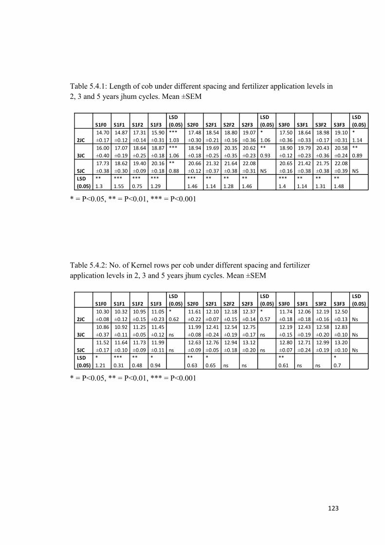
123
Table 5.4.1: Length of cob under different spacing and fertilizer application levels in2, 3 and 5 years jhum cycles. Mean ±SEM
* = P<0.05, ** = P<0.01, *** = P<0.001
Table 5.4.2: No. of Kernel rows per cob under different spacing and fertilizerapplication levels in 2, 3 and 5 years jhum cycles. Mean ±SEM
* = P<0.05, ** = P<0.01, *** = P<0.001
S1F0 S1F1 S1F2 S1F3LSD(0.05) S2F0 S2F1 S2F2 S2F3
LSD(0.05) S3F0 S3F1 S3F2 S3F3
LSD(0.05)
2JC14.70±0.17
14.87±0.12
17.31±0.14
15.90±0.31
***1.03
17.48±0.30
18.54±0.21
18.80±0.16
19.07±0.36
*1.06
17.50±0.36
18.64±0.33
18.98±0.17
19.10±0.31
*1.14
3JC16.00±0.40
17.07±0.19
18.64±0.25
18.87±0.18
***1.06
18.94±0.18
19.69±0.25
20.35±0.35
20.62±0.23
**0.93
18.90±0.12
19.79±0.23
20.43±0.36
20.58±0.24
**0.89
5JC17.73±0.38
18.62±0.30
19.40±0.09
20.16±0.18
**0.88
20.66±0.12
21.32±0.37
21.64±0.38
22.08±0.31 NS
20.65±0.16
21.42±0.38
21.75±0.38
22.08±0.39 NS
LSD(0.05)
**1.3
***1.55
***0.75
***1.29
***1.46
**1.14
**1.28
**1.46
***1.4
**1.14
**1.31
**1.48
S1F0 S1F1 S1F2 S1F3LSD(0.05) S2F0 S2F1 S2F2 S2F3
LSD(0.05) S3F0 S3F1 S3F2 S3F3
LSD(0.05)
2JC10.30±0.08
10.32±0.12
10.95±0.15
11.05±0.23
*0.62
11.61±0.22
12.10±0.07
12.18±0.15
12.37±0.14
*0.57
11.74±0.18
12.06±0.18
12.19±0.16
12.50±0.13 Ns
3JC10.86±0.37
10.92±0.11
11.25±0.05
11.45±0.12 ns
11.99±0.08
12.41±0.24
12.54±0.19
12.75±0.17 ns
12.19±0.15
12.43±0.19
12.58±0.20
12.83±0.10 Ns
5JC11.52±0.17
11.64±0.10
11.73±0.09
11.99±0.11 ns
12.63±0.09
12.76±0.05
12.94±0.18
13.12±0.20 ns
12.80±0.07
12.71±0.24
12.99±0.19
13.20±0.10 Ns
LSD(0.05)
*1.21
***0.31
**0.48
*0.94
**0.63
*0.65 ns ns
**0.61 ns ns
*0.7

124
Figure 5.4.3 Effect of fertilizer application on kernels per row under different spacingin 2 years, 3 years and 5 years jhum cycles. Vertical line indicates standard error.
Figure 5.4.4 Effect of fertilizer application on kernels per cob under different spacingin 2 years, 3 years and 5 years jhum cycles. Vertical line indicates standard error.

125
Table 5.4.3: The effect of fertilizer application on number of kernels per row under S1, S2and S3 spacing in 2, 3 and 5 years jhum cycles. Mean ±SEM
* = P<0.05, ** = P<0.01, *** = P<0.001
Table 5.4.4: The effect of fertilizer application on number of kernels per cob under S1, S2and S3 spacing in 2, 3 and 5 years jhum cycles. Mean ±SEM
* = P<0.05, ** = P<0.01, *** = P<0.001
S1F0 S1F1 S1F2 S1F3LSD(0.05) S2F0 S2F1 S2F2 S2F3
LSD(0.05) S3F0 S3F1 S3F2 S3F3
LSD(0.05)
2JC26.24±0.48
27.38±0.35
27.56±0.17
27.75±0.18
*1.13
31.75±0.33
31.63±0.17
32.79±0.32
33.20±0.61 NS
31.42±0.10
31.79±0.21
32.90±0.33
33.44±0.34
**1.11
3JC28.96±0.34
29.14±0.08
29.43±0.26
30.90±0.10
***1.46
34.59±0.11
35.01±0.33
35.57±0.22
36.11±0.14
**0.97
34.51±0.11
35.05±0.13
35.53±0.22
35.60±0.17
**0.53
5JC32.40±0.12
31.63±0.19
32.31±0.16
32.90±0.29
*0.68
36.67±0.19
37.20±0.20
38.17±0.04
38.58±0.22
***0.96
36.70±0.38
37.39±0.11
38.10±0.08
38.53±0.30
**1.14
LSD(0.05)
***2.71
***1.76
***1.87
***2
***2.07
***2.19
***2.6
***2.47
***2.18
***2.34
***2.57
***2.15
S1F0 S1F1 S1F2 S1F3LSD(0.05) S2F0 S2F1 S2F2 S2F3
LSD(0.05) S3F0 S3F1 S3F2 S3F3
LSD(0.05)
2JC270.44±7.03
282.69±5.67
301.63±2.25
306.59±6.78
**18.94
368.47±3.82
382.71±1.52
399.30±2.47
410.65±3.14
***11.35
368.99±5.35
383.21±3.28
401.05±6.54
417.93±2.61
***16.88
3JC317.57±14.90
318.11±3.03
331.03±3.30
353.72±4.86
*35.61
414.76±3.48
434.43±4.46
445.97±7.62
460.25±4.50
**19.62
420.62±6.33
435.73±8.29
446.95±4.26
456.77±5.34
*21.04
5JC373.21±4.22
368.13±4.99
378.91±1.97
394.36±4.96
*15.45
462.95±1.90
474.68±3.50
494.04±6.71
506.11±5.16
***19.36
469.83±2.47
475.05±8.06
494.90±7.86
508.71±0.72
**19.85
LSD(0.05)
***47.12
***33.42
***29.4
***40.63
***46.28
***40.24
***46.67
***45.86
***49.21
***39.31
***45.9
***38.84
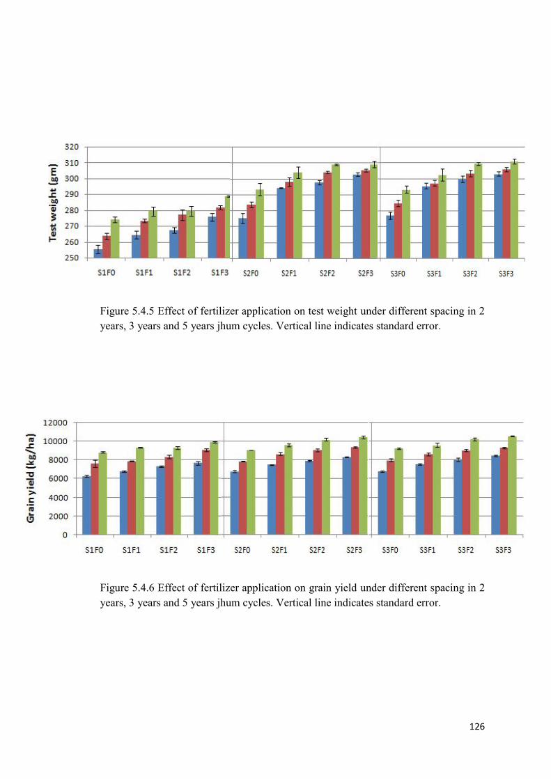
126
Figure 5.4.5 Effect of fertilizer application on test weight under different spacing in 2years, 3 years and 5 years jhum cycles. Vertical line indicates standard error.
Figure 5.4.6 Effect of fertilizer application on grain yield under different spacing in 2years, 3 years and 5 years jhum cycles. Vertical line indicates standard error.
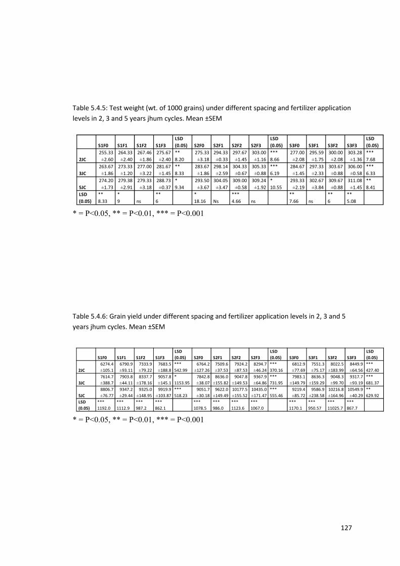
127
Table 5.4.5: Test weight (wt. of 1000 grains) under different spacing and fertilizer applicationlevels in 2, 3 and 5 years jhum cycles. Mean ±SEM
* = P<0.05, ** = P<0.01, *** = P<0.001
Table 5.4.6: Grain yield under different spacing and fertilizer application levels in 2, 3 and 5years jhum cycles. Mean ±SEM
* = P<0.05, ** = P<0.01, *** = P<0.001
S1F0 S1F1 S1F2 S1F3LSD(0.05) S2F0 S2F1 S2F2 S2F3
LSD(0.05) S3F0 S3F1 S3F2 S3F3
LSD(0.05)
2JC255.33±2.60
264.33±2.40
267.46±1.86
275.67±2.40
**8.20
275.33±3.18
294.33±0.33
297.67±1.45
303.00±1.16
***8.66
277.00±2.08
295.59±1.75
300.00±2.08
303.28±1.36
***7.68
3JC263.67±1.86
273.33±1.20
277.00±3.22
281.67±1.45
**8.33
283.67±1.86
298.14±2.59
304.33±0.67
305.33±0.88
***6.19
284.67±1.45
297.33±2.33
303.67±0.88
306.00±0.58
***6.33
5JC274.20±1.73
279.38±2.91
279.33±3.18
288.73±0.37
*9.34
293.50±3.67
304.05±3.47
309.00±0.58
309.24±1.92
*10.55
293.33±2.19
302.67±3.84
309.67±0.88
311.08±1.45
**8.41
LSD(0.05)
**8.33
*9 ns
**6
*18.16 Ns
***4.66 ns
**7.66 ns
**6
**5.08
S1F0 S1F1 S1F2 S1F3LSD(0.05) S2F0 S2F1 S2F2 S2F3
LSD(0.05) S3F0 S3F1 S3F2 S3F3
LSD(0.05)
2JC6274.4±105.1
6790.9±93.11
7333.9±79.22
7683.5±188.8
***542.99
6764.2±127.26
7509.6±37.53
7924.2±87.53
8294.7±46.24
***370.16
6812.9±77.69
7551.3±75.17
8022.5±183.99
8449.9±64.56
***427.40
3JC7614.7±388.7
7903.8±44.11
8337.7±178.16
9057.8±145.1
*1153.95
7842.8±38.07
8636.0±155.82
9047.8±149.53
9367.9±64.86
***731.95
7983.1±149.79
8636.3±159.29
9048.3±99.70
9317.7±93.19
***681.37
5JC8806.7±76.77
9347.2±29.44
9325.0±148.95
9919.9±103.87
***518.23
9051.7±30.18
9622.0±149.49
10177.5±155.52
10435.0±171.47
***555.46
9219.4±85.72
9586.9±238.58
10216.8±164.96
10549.9±40.29
**629.92
LSD(0.05)
***1192.0
***1112.9
***987.2
***862.1
***1078.5
***986.0
***1123.6
***1067.0
***1170.1
***950.57
***11025.7
***867.7
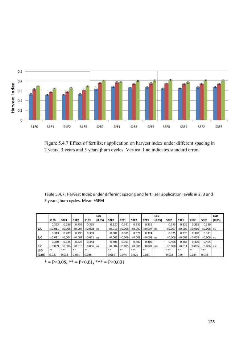
128
Figure 5.4.7 Effect of fertilizer application on harvest index under different spacing in2 years, 3 years and 5 years jhum cycles. Vertical line indicates standard error.
Table 5.4.7: Harvest Index under different spacing and fertilizer application levels in 2, 3 and5 years jhum cycles. Mean ±SEM
* = P<0.05, ** = P<0.01, *** = P<0.001
S1F0 S1F1 S1F2 S1F3LSD(0.05) S2F0 S2F1 S2F2 S2F3
LSD(0.05) S3F0 S3F1 S3F2 S3F3
LSD(0.05)
2JC0.262
±0.0110.256
±0.0060.259
±0.0040.265
±0.008 ns0.320
±0.0190.341
±0.0080.332
±0.0020.335
±0.007 ns0.323
±0.0070.326
±0.0020.335
±0.0100.339
±0.006 ns
3JC0.313
±0.0110.289
±0.0040.290
±0.0070.309
±0.011 ns0.381
±0.0070.385
±0.0090.371
±0.0080.374
±0.008 ns0.375
±0.0060.370
±0.0070.370
±0.0050.371
±0.006 ns
5JC0.350
±0.0090.325
±0.0060.328
±0.0100.348
±0.006 ns0.405
±0.0040.391
±0.0050.400
±0.0060.405
±0.007 ns0.408
±0.0080.385
±0.0110.406
±0.0050.405
±0.006 nsLSD(0.05)
**0.037
***0.033
**0.031
**0.038
**0.061
**0.044
***0.029
**0.031
***0.033
**0.04
**0.034
***0.031

129
5.5 Effect of plant spacing on growth parameters
5.5.1 Plant height at 15 DAS
The height at 15 DAS showed no significant (P<0.05) effect except in
F0 plot in 5JC. Although there was no statistical significance, plants grown under S1
spacing showed comparatively plant height (Figure 5.5.1 & Table 5.5.1).
5.5.2 Plant height at 30 DAS
Plant height at 30DAS showed more significance difference among the
S1, S2 and S3 spacings of each fertilizer treatments. In 2JC, significant difference was
observed among different spacings with F2 level of fertilizer application. In 3JC,
significant difference was observed among different spacings of F0 and F2 fertilizer
levels. In 5JC, significance effect of plant spacing was observed under each of the
fertilizer levels. In all the Fertilizer levels, F2 and F3 showed comparable values
where as plants in S1 showed significantly lower plant height (Figure 5.5.2 & Table
5.5.2).
5.5.3 Plant height at 45 DAS
Plant height at 45DAS also showed low significant response to plant
spacing. Significant difference (P<0.05) in height occurred among the spacings of all
the fertilizer levels. In all the jhum cycles, lowest height occurred in highest plant
density where as similar values were observed between S2 and S3 spacings (Table
5.5.3 & Figure 5.5.3).
5.5.4 Plant height at 60 DAS
At 60DAS, significant difference (P<0.05) among the three spacing
was observed in all the fertilizer levels of 2JC, 3JC and 5JC. The significant different
was due to the wide range between S1 to S2 and S3, and no significant difference was
observed between S2 and S3. From all the combinations of spacings and fertilizer
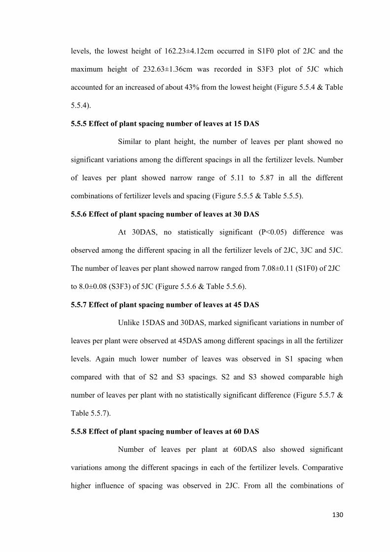
130
levels, the lowest height of 162.23±4.12cm occurred in S1F0 plot of 2JC and the
maximum height of 232.63±1.36cm was recorded in S3F3 plot of 5JC which
accounted for an increased of about 43% from the lowest height (Figure 5.5.4 & Table
5.5.4).
5.5.5 Effect of plant spacing number of leaves at 15 DAS
Similar to plant height, the number of leaves per plant showed no
significant variations among the different spacings in all the fertilizer levels. Number
of leaves per plant showed narrow range of 5.11 to 5.87 in all the different
combinations of fertilizer levels and spacing (Figure 5.5.5 & Table 5.5.5).
5.5.6 Effect of plant spacing number of leaves at 30 DAS
At 30DAS, no statistically significant (P<0.05) difference was
observed among the different spacing in all the fertilizer levels of 2JC, 3JC and 5JC.
The number of leaves per plant showed narrow ranged from 7.08±0.11 (S1F0) of 2JC
to 8.0±0.08 (S3F3) of 5JC (Figure 5.5.6 & Table 5.5.6).
5.5.7 Effect of plant spacing number of leaves at 45 DAS
Unlike 15DAS and 30DAS, marked significant variations in number of
leaves per plant were observed at 45DAS among different spacings in all the fertilizer
levels. Again much lower number of leaves was observed in S1 spacing when
compared with that of S2 and S3 spacings. S2 and S3 showed comparable high
number of leaves per plant with no statistically significant difference (Figure 5.5.7 &
Table 5.5.7).
5.5.8 Effect of plant spacing number of leaves at 60 DAS
Number of leaves per plant at 60DAS also showed significant
variations among the different spacings in each of the fertilizer levels. Comparative
higher influence of spacing was observed in 2JC. From all the combinations of

131
spacing and fertilizer levels, lowest number of leaves per plant occurred in
10.82±0.03 (S1F0) in 2JC and highest number in 13.68±0.07 (S3F2) of 5JC which
accounted for an increase of about 26% (Figure 5.5.8 & Table 5.5.8).
5.5.9 Biomass production
The plant biomass at the time of maturity harvest in terms of dry weight showed
significant variations among the S1, S2 and S3 spacings in all the fertilizer levels of
2JC, 3JC and 5JC. Similar to plant height and number of leaves per plant, plants in S1
spacing showed comparatively lower biomass production and similar values were
observed in S2 and S3. The lowest plant biomass of 264.50±7.37 gm (S1F0) of 2JC to
the highest of 390.93±4.29gm (S3F3) of 5JC accounted for 47.79% increase from the
lowest value (Figure 5.5.9 & Table 5.5.9).
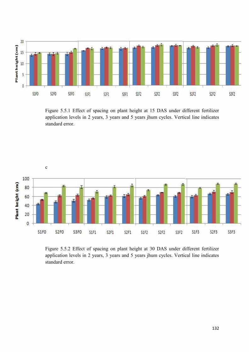
132
Figure 5.5.1 Effect of spacing on plant height at 15 DAS under different fertilizerapplication levels in 2 years, 3 years and 5 years jhum cycles. Vertical line indicatesstandard error.
c
Figure 5.5.2 Effect of spacing on plant height at 30 DAS under different fertilizerapplication levels in 2 years, 3 years and 5 years jhum cycles. Vertical line indicatesstandard error.

133
Table 5.5.1: Effect of spacing on plant height at 15DAS under different levels offertilizer applications in 2, 3 and 5 years jhum cycles. Mean ±SEM.
* = P<0.05, ** = P<0.01, *** = P<0.001
Table 5.5.2: Effect of spacing on plant height at 30DAS under different levels offertilizer applications in 2, 3 and 5 years jhum cycles. Mean ±SEM.
* = P<0.05, ** = P<0.01, *** = P<0.001
S1F0 S2F0 S3F0LSD(0.05) S1F1 S2F1 S3F1
LSD(0.05) S1F2 S2F2 S3F2
LSD(0.05) S1F3 S2F3 S3F3
LSD(0.05)
2JC13.85±0.46
14.43±0.48
14.48±0.67 ns
15.80±0.11
16.78±0.48
16.70±0.60 ns
17.16±0.36
17.30±0.34
17.97±0.29 ns
18.14±0.56
18.10±0.23
18.39±0.28
ns
3JC14.44±0.53
14.37±0.62
15.14±0.48 ns
16.91±0.16
17.20±0.31
16.91±0.34 ns
17.98±0.34
18.19±0.30
18.27±0.47 ns
18.54±0.33
18.89±0.23
18.86±0.44
ns
5JC14.90±0.12
14.78±0.35
16.87±0.18
**1.96
16.72±0.54
17.07±0.41
17.11±0.34 ns
17.44±0.42
18.52±0.52
18.13±0.14 ns
18.63±0.29
19.11±0.20
18.97±0.13
ns
S1F0 S2F0 S3F0LSD(0.05) S1F1 S2F1 S3F1
LSD(0.05) S1F2 S2F2 S3F2
LSD(0.05) S1F3 S2F3 S3F3
LSD(0.05)
2JCSEM
43.16±1.95
48.18±1.90
50.87±2.94 ns
52.88±1.96
59.57±2.32
61.59±2.94 ns
56.60±1.34
63.62±1.66
61.30±SEM
*7.01
60.66±2.71
66.94±1.81
65.69±1.73
ns
3JCSEM
52.72±1.57
61.76±2.21
63.46±1.96
*9.03
56.83±1.36
62.53±1.60
64.90±2.43 ns
61.27±0.51
69.63±1.24
68.67±SEM
**7.40
63.70±1.96
71.41±3.18
70.44±3.39
ns
5JCSEM
68.28±1.40
83.79±1.54
81.30±3.01
**13.01
71.14±2.70
82.32±2.09
84.83±3.27
*11.17
74.67±1.35
87.18±1.83
87.69±SEM
**12.51
79.87±1.15
89.38±1.57
89.56±1.57
**9.51

134
Figure 5.5.3 Effect of spacing on plant height at 45 DAS under different fertilizerapplication levels in 2 years, 3 years and 5 years jhum cycles. Vertical line indicatesstandard error.
Figure 5.5.4 Effect of spacing on plant height at 60 DAS under different fertilizerapplication levels in 2 years, 3 years and 5 years jhum cycles. Vertical line indicatesstandard error.

135
Table 5.5.3: Effect of spacing on plant height at 45DAS under different levels offertilizer applications in 2, 3 and 5 years jhum cycles. Mean ±SEM.
* = P<0.05, ** = P<0.01, *** = P<0.001
Table 5.5.4: Effect of spacing on plant height at 60DAS under different levels offertilizer applications in 2, 3 and 5 years jhum cycles. Mean ±SEM.
* = P<0.05, ** = P<0.01, *** = P<0.001
S1F0 S2F0 S3F0LSD(0.05) S1F1 S2F1 S3F1
LSD(0.05) S1F2 S2F2 S3F2
LSD(0.05) S1F3 S2F3 S3F3
LSD(0.05)
2JC79.74±0.84
85.64±1.56
83.55±1.09
*5.90
89.46±0.85
100.03±3.37
98.28±2.38
*8.81
97.52±4.27
112.10±4.15
115.34±3.51
*2.58
101.92±2.01
118.50±4.15
122.42±6.62
*16.58
3JC89.60±3.32
97.83±2.92
106.73±2.98
*17.13
101.63±1.61
103.21±2.47
111.11±3.35 ns
109.35±1.43
118.93±2.37
122.84±2.54
*9.57
121.42±0.78
131.67±4.49
131.26±1.24 ns
5JC142.34±3.56
159.81±3.50
153.94±2.40
*11.60
157.08±2.65
166.56±2.89
168.37±1.20
*9.47
163.85±1.81
171.34±4.21
175.67±1.45 ns
170.67±2.03
184.26±3.14
181.31±1.22
*10.64
S1F0 S2F0 S3F0LSD(0.05) S1F1 S2F1 S3F1
LSD(0.05) S1F2 S2F2 S3F2
LSD(0.05) S1F3 S2F3 S3F3
LSD(0.05)
2JC162.23±4.12
185.61±3.38
188.32±1.48
**23.37
169.03±3.84
195.74±3.36
197.45±4.72
**26.71
177.50±5.02
207.87±2.62
206.25±1.92
**28.75
184.63±5.14
215.34±2.49
212.72±3.29
**28.08
3JC165.38±2.10
190.51±5.36
193.98±2.55
**25.13
177.44±5.60
200.58±1.64
202.05±2.01
**23.13
186.50±4.55
210.98±2.39
209.45±4.19
**22.94
196.14±5.32
218.72±1.00
217.52±2.60
**21.37
5JC183.33±3.84
205.52±2.04
206.89±1.42
**22.18
194.88±3.47
212.32±2.92
211.03±1.84
**16.15
201.41±4.70
217.45±2.10
217.83±2.27 *
212.54±1.36
229.92±0.28
232.63±1.36
***17.37

136
Figure 5.5.5 Effect of spacing on number of leaves per plant at 15 DAS underdifferent fertilizer application levels in 2 years, 3 years and 5 years jhum cycles.Vertical line indicates standard error.
Figure 5.5.6 Effect of spacing on number of leaves per plant at 30 DAS underdifferent fertilizer application levels in 2 years, 3 years and 5 years jhum cycles.Vertical line indicates standard error.
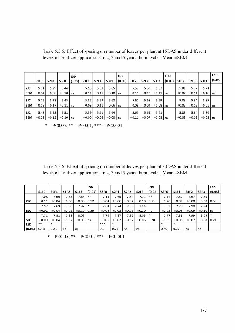
137
Table 5.5.5: Effect of spacing on number of leaves per plant at 15DAS under differentlevels of fertilizer applications in 2, 3 and 5 years jhum cycles. Mean ±SEM.
* = P<0.05, ** = P<0.01, *** = P<0.001
Table 5.5.6: Effect of spacing on number of leaves per plant at 30DAS under differentlevels of fertilizer applications in 2, 3 and 5 years jhum cycles. Mean ±SEM.
* = P<0.05, ** = P<0.01, *** = P<0.001
S1F0 S2F0 S3F0LSD(0.05) S1F1 S2F1 S3F1
LSD(0.05) S1F2 S2F2 S3F2
LSD(0.05) S1F3 S2F3 S3F3
LSD(0.05)
2JCSEM
5.11±0.04
5.29±0.08
5.44±0.10 ns
5.55±0.11
5.58±0.11
5.65±0.10 ns
5.57±0.11
5.63±0.13
5.67±0.11 ns
5.81±0.07
5.77±0.11
5.71±0.10 ns
3JCSEM
5.15±0.09
5.23±0.17
5.45±0.11 ns
5.55±0.09
5.59±0.11
5.62±0.06 ns
5.61±0.09
5.68±0.04
5.69±0.08 ns
5.83±0.03
5.84±0.03
5.87±0.05 ns
5JCSEM
5.48±0.06
5.53±0.12
5.58±0.10 ns
5.59±0.09
5.61±0.06
5.64±0.08 ns
5.65±0.11
5.69±0.07
5.71±0.08 ns
5.83±0.03
5.84±0.03
5.86±0.03 ns
S1F0 S1F1 S1F2 S1F3LSD(0.05) S2F0 S2F1 S2F2 S2F3
LSD(0.05) S3F0 S3F1 S3F2 S3F3
LSD(0.05)
2JC7.08
±0.117.60
±0.047.65
±0.087.68
±0.08**0.52
7.13±0.04
7.65±0.06
7.64±0.07
7.71±0.10
**0.51
7.14±0.20
7.67±0.07
7.67±0.08
7.69±0.08
*0.53
3JC7.57
±0.027.69
±0.047.86
±0.097.92
±0.10*0.29
7.64±0.02
7.74±0.03
7.88±0.09
7.94±0.10 ns
7.63±0.02
7.77±0.03
7.90±0.09
7.94±0.10 ns
5JC7.71
±0.097.82
±0.047.91
±0.078.02
±0.08 ns7.76
±0.067.87
±0.027.96
±0.078.03
±0.06*0.20
7.77±0.05
7.89±0.00
7.99±0.07
8.05±0.08
*0.21
LSD(0.05)
**0.48
*0.21 ns ns
***0.5
*0.21 ns ns
*0.49
*0.22 ns ns

138
Figure 5.5.7 Effect of spacing on number of leaves per plant at 45 DAS underdifferent fertilizer application levels in 2 years, 3 years and 5 years jhum cycles.Vertical line indicates standard error.
Figure 5.5.8 Effect of spacing on number of leaves per plant at 60 DAS underdifferent fertilizer application levels in 2 years, 3 years and 5 years jhum cycles.Vertical line indicates standard error.

139
Table 5.5.7: Effect of spacing on number of leaves per plant at 45DAS under differentlevels of fertilizer applications in 2, 3 and 5 years jhum cycles. Mean ±SEM.
* = P<0.05, ** = P<0.01, *** = P<0.001
Table 5.5.8: Effect of spacing on number of leaves per plant at 60DAS under differentlevels of fertilizer applications in 2, 3 and 5 years jhum cycles. Mean ±SEM.
*= P<0.05, ** = P<0.01, *** = P<0.001
S1F0 S2F0 S3F0LSD(0.05) S1F1 S2F1 S3F1
LSD(0.05) S1F2 S2F2 S3F2
LSD(0.05) S1F3 S2F3 S3F3
LSD(0.05)
2JC 9.85±0.31
10.98±0.25
11.13±0.15
*1.12
10.13±0.36
11.48±0.15
11.50±0.05
**1.34
10.39±0.07
11.53±0.14
11.63±0.14
***1.14
10.87±0.20
11.59±0.17
11.61±0.03
*0.71
3JC 10.15±0.13
11.40±0.03
11.45±0.06
***1.25
10.37±0.10
11.57±0.05
11.68±0.01
***1.20
10.68±0.07
11.74±0.02
11.78±0.03
***1.05
11.00±0.15
11.80±0.09
11.81±0.09
**0.79
5JC 10.37±0.09
11.84±0.01
11.83±0.05
***17.43
11.20±0.15
11.92±0.02
12.01±0.06
**0.71
11.30±0.06
12.10±0.10
12.11±0.08
***0.80
11.67±0.07
12.25±0.03
12.21±0.04
***0.54
S1F0 S1F1 S1F2 S1F3LSD(0.05) S2F0 S2F1 S2F2 S2F3
LSD(0.05) S3F0 S3F1 S3F2 S3F3
LSD(0.05)
2JC10.59±0.17
10.71±0.28
11.25±0.07
11.50±0.09
*0.65
11.98±0.05
12.35±0.05
12.34±0.06
12.56±0.02
***0.21
12.09±0.06
12.34±0.02
12.41±0.04
12.55±0.06
**0.21
3JC10.49±0.36
10.69±0.32
10.97±0.24
11.17±0.05 ns
12.06±0.15
12.44±0.30
12.54±0.37
12.78±0.34 ns
12.18±0.11
12.45±0.33
12.58±0.27
12.99±0.25 ns
5JC10.87±0.34
11.32±0.07
11.98±0.17
12.34±0.14
**1.02
12.48±0.28
12.75±0.31
13.24±0.15
13.68±0.07
*0.76
12.27±0.54
12.80±0.30
13.25±0.18
13.66±0.05 ns
LSD(0.05) ns ns
*0.73
***0.84 ns ns ns
*0.9 ns ns
*0.67
**0.67

140
Figure 5.5.9 Effect of spacing on biomass production at maturity harvest underdifferent fertilizer application levels in 2 years, 3 years and 5 years jhum cycles.Vertical line indicates standard error
Table 5.5.9: Effect of spacing on biomass production at maturity harvest underdifferent levels of fertilizer application in 2, 3 and 5 years jhum cycles. Mean ±SEM
*= P<0.05, ** = P<0.01, *** = P<0.001
S1F0 S2F0 S3F0LSD(0.05) S1F1 S2F1 S3F1
LSD(0.05) S1F2 S2F2 S3F2
LSD(0.05) S1F3 S2F3 S3F3
LSD(0.05)
2JC 264.50±7.37
318.50±14.40
316.50±3.97
*52
292.50±7.70
331.00±6.61
347.00±3.50
**38.5
311.50±4.44
358.50±4.58
359.65±3.16
***47
319.50±3.12
371.50±6.08
374.20±4.09
***52
3JC 267.77±4.91
308.55±3.87
319.66±3.01
***40.78
301.12±2.11
336.59±2.24
350.15±3.33
***13.55
316.10±3.02
366.17±2.34
367.19±1.37
***50.07
322.38±6.39
376.03±5.67
377.08±2.28
***53.64
5JC 292.60±4.50
335.80±2.75
337.72±2.78
***43.19
316.87±5.96
369.59±2.84
373.41±3.95
***52.72
323.40±5.30
381.54±2.01
377.46±2.96
***54.05
327.13±5.96
386.11±1.79
390.93±4.29
***58.98
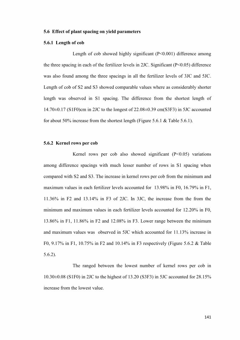
141
5.6 Effect of plant spacing on yield parameters
5.6.1 Length of cob
Length of cob showed highly significant (P<0.001) difference among
the three spacing in each of the fertilizer levels in 2JC. Significant (P<0.05) difference
was also found among the three spacings in all the fertilizer levels of 3JC and 5JC.
Length of cob of S2 and S3 showed comparable values where as considerably shorter
length was observed in S1 spacing. The difference from the shortest length of
14.70±0.17 (S1F0)cm in 2JC to the longest of 22.08±0.39 cm(S3F3) in 5JC accounted
for about 50% increase from the shortest length (Figure 5.6.1 & Table 5.6.1).
5.6.2 Kernel rows per cob
Kernel rows per cob also showed significant (P<0.05) variations
among difference spacings with much lesser number of rows in S1 spacing when
compared with S2 and S3. The increase in kernel rows per cob from the minimum and
maximum values in each fertilizer levels accounted for 13.98% in F0, 16.79% in F1,
11.36% in F2 and 13.14% in F3 of 2JC. In 3JC, the increase from the from the
minimum and maximum values in each fertilizer levels accounted for 12.20% in F0,
13.86% in F1, 11.86% in F2 and 12.08% in F3. Lower range between the minimum
and maximum values was observed in 5JC which accounted for 11.13% increase in
F0, 9.17% in F1, 10.75% in F2 and 10.14% in F3 respectively (Figure 5.6.2 & Table
5.6.2).
The ranged between the lowest number of kernel rows per cob in
10.30±0.08 (S1F0) in 2JC to the highest of 13.20 (S3F3) in 5JC accounted for 28.15%
increase from the lowest value.
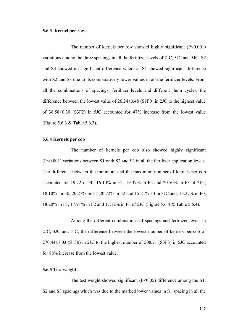
142
5.6.3 Kernel per row
The number of kernels per row showed highly significant (P<0.001)
variations among the three spacings in all the fertilizer levels of 2JC, 3JC and 5JC. S2
and S3 showed no significant difference where as S1 showed significant difference
with S2 and S3 due to its comparatively lower values in all the fertilizer levels. From
all the combinations of spacings, fertilizer levels and different jhum cycles, the
difference between the lowest value of 26.24±0.48 (S1F0) in 2JC to the highest value
of 38.58±0.30 (S3F2) in 5JC accounted for 47% increase from the lowest value
(Figure 5.6.3 & Table 5.6.3).
5.6.4 Kernels per cob
The number of kernels per cob also showed highly significant
(P<0.001) variations between S1 with S2 and S3 in all the fertilizer application levels.
The difference between the minimum and the maximum number of kernels per cob
accounted for 19.72 in F0, 16.10% in F1, 19.37% in F2 and 20.50% in F3 of 2JC;
18.10% in F0, 20.27% in F1, 20.72% in F2 and 15.21% F3 in 3JC and, 13.27% in F0,
18.20% in F1, 17.91% in F2 and 17.12% in F3 of 5JC (Figure 5.6.4 & Table 5.6.4).
Among the different combinations of spacings and fertilizer levels in
2JC, 3JC and 5JC, the difference between the lowest number of kernels per cob of
270.44±7.03 (S1F0) in 2JC to the highest number of 508.71 (S3F3) in 5JC accounted
for 88% increase from the lowest value.
5.6.5 Test weight
The test weight showed significant (P<0.05) difference among the S1,
S2 and S3 spacings which was due to the marked lower values in S1 spacing in all the
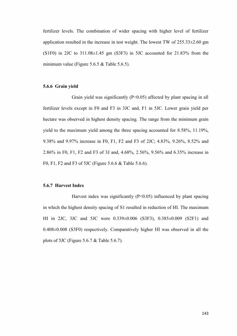
143
fertilizer levels. The combination of wider spacing with higher level of fertilizer
application resulted in the increase in test weight. The lowest TW of 255.33±2.60 gm
(S1F0) in 2JC to 311.08±1.45 gm (S3F3) in 5JC accounted for 21.83% from the
minimum value (Figure 5.6.5 & Table 5.6.5).
5.6.6 Grain yield
Grain yield was significantly (P<0.05) affected by plant spacing in all
fertilizer levels except in F0 and F3 in 3JC and, F1 in 5JC. Lower grain yield per
hectare was observed in highest density spacing. The range from the minimum grain
yield to the maximum yield among the three spacing accounted for 8.58%, 11.19%,
9.38% and 9.97% increase in F0, F1, F2 and F3 of 2JC; 4.83%, 9.26%, 8.52% and
2.86% in F0, F1, F2 and F3 of 3J and, 4.68%, 2.56%, 9.56% and 6.35% increase in
F0, F1, F2 and F3 of 5JC (Figure 5.6.6 & Table 5.6.6).
5.6.7 Harvest Index
Harvest index was significantly (P<0.05) influenced by plant spacing
in which the highest density spacing of S1 resulted in reduction of HI. The maximum
HI in 2JC, 3JC and 5JC were 0.339±0.006 (S3F3), 0.385±0.009 (S2F1) and
0.408±0.008 (S3F0) respectively. Comparatively higher HI was observed in all the
plots of 5JC (Figure 5.6.7 & Table 5.6.7).

144
Figure 5.6.1 Effect of spacing on length of cob under different fertilizer applicationlevels in 2 years, 3 years and 5 years jhum cycles. Vertical line indicates standarderror
Figure 5.6.2 Effect of spacing on kernel rows per cob under different fertilizerapplication levels in 2 years, 3 years and 5 years jhum cycles. Vertical line indicatesstandard error

145
Table 5.6.1: Effect of spacing on length of cob under different levels of fertilizer applicationin 2, 3 and 5 years jhum cycles. Mean ±SEM
* = P<0.05, ** = P<0.01, *** = P<0.001
Table 5.6.2: Effect of spacing on kernel rows per cob under different levels of fertilizerapplication in 2, 3 and 5 years jhum cycles. Mean ±SEM.
* = P<0.05, ** = P<0.01, *** = P<0.001
S1F0 S2F0 S3F0LSD(0.05) S1F1 S2F1 S3F1
LSD(0.05) S1F2 S2F2 S3F2
LSD(0.05) S1F3 S2F3 S3F3
LSD(0.05)
2JC 14.70±0.17
17.48±0.30
17.50±0.36
***2.77
14.87±0.12
18.54±0.21
18.64±0.33
***3.67
17.31±0.14
18.80±0.16
18.98±0.17
***1.49
15.90±0.31
19.07±0.36
19.10±0.31
***3.16
3JC 16.00±0.40
18.94±0.18
18.90±0.12
***2.9
17.07±0.19
19.69±0.25
19.79±0.23
***2.62
18.64±0.25
20.35±0.35
20.43±0.36
*1.71
18.87±0.18
20.62±0.23
20.58±0.24
**1.71
5JC 17.73±0.38
20.66±0.12
20.65±0.16
***2.91
18.62±0.30
21.32±0.37
21.42±0.38
**2.69
19.40±0.09
21.64±0.38
21.75±0.38
**2.23
20.16±0.18
22.08±0.31
22.08±0.39
**1.91
S1F0 S2F0 S3F0LSD(0.05) S1F1 S2F1 S3F1
LSD(0.05) S1F2 S2F2 S3F2
LSD(0.05) S1F3 S2F3 S3F3
LSD(0.05)
2JC 10.30±0.08
11.61±0.22
11.74±0.18
**1.30
10.32±0.12
12.10±0.07
12.06±0.18
***1.73
10.95±0.15
12.18±0.15
12.19±0.16
**1.23
11.05±0.23
12.37±0.14
12.50±0.13
**1.32
3JC 10.86±0.37
11.99±0.08
12.19±0.15
*1.12
10.92±0.11
12.41±0.24
12.43±0.19
**1.49
11.25±0.05
12.54±0.19
12.58±0.20
**1.29
11.45±0.12
12.75±0.17
12.83±0.10
***1.30
5JC 11.52±0.17
12.63±0.09
12.80±0.07
***1.10
11.64±0.10
12.76±0.05
12.71±0.24
**1.06
11.73±0.09
12.94±0.18
12.99±0.19
**1.21
11.99±0.11
13.12±0.20
13.20±0.10
**1.13
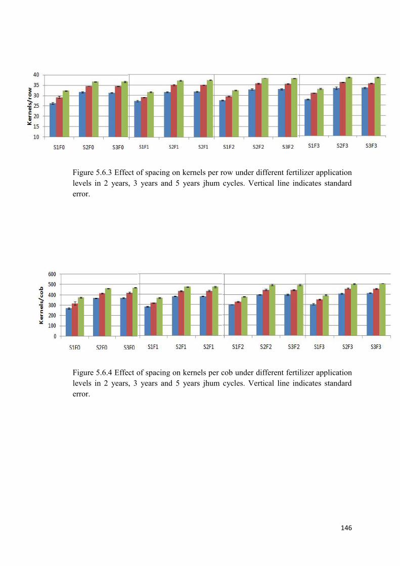
146
Figure 5.6.3 Effect of spacing on kernels per row under different fertilizer applicationlevels in 2 years, 3 years and 5 years jhum cycles. Vertical line indicates standarderror.
Figure 5.6.4 Effect of spacing on kernels per cob under different fertilizer applicationlevels in 2 years, 3 years and 5 years jhum cycles. Vertical line indicates standarderror.

147
Table5.6.3: Effect of spacing on kernel per row under different levels of fertilizer applicationin 2, 3 and 5 years Jhum cycles. Mean ±SEM
* = P<0.05, ** = P<0.01, *** = P<0.001
Table5.6.4: Effect of spacing on kernel per cob under different levels of fertilizer applicationin 2, 3 and 5 years jhum cycles. Mean ±SEM
* = P<0.05, ** = P<0.01, *** = P<0.001
S1F0 S2F0 S3F0LSD(0.05) S1F1 S2F1 S3F1
LSD(0.05) S1F2 S2F2 S3F2
LSD(0.05) S1F3 S2F3 S3F3
LSD(0.05)
2JC 10.30±0.08
11.61±0.22
11.74±0.18
**1.30
10.32±0.12
12.10±0.07
12.06±0.18
***1.73
10.95±0.15
12.18±0.15
12.19±0.16
**1.23
11.05±0.23
12.37±0.14
12.50±0.13
**1.32
3JC 10.86±0.37
11.99±0.08
12.19±0.15
*1.12
10.92±0.11
12.41±0.24
12.43±0.19
**1.49
11.25±0.05
12.54±0.19
12.58±0.20
**1.29
11.45±0.12
12.75±0.17
12.83±0.10
***1.30
5JC 11.52±0.17
12.63±0.09
12.80±0.07
***1.10
11.64±0.10
12.76±0.05
12.71±0.24
**1.06
11.73±0.09
12.94±0.18
12.99±0.19
**1.21
11.99±0.11
13.12±0.20
13.20±0.10
**1.13
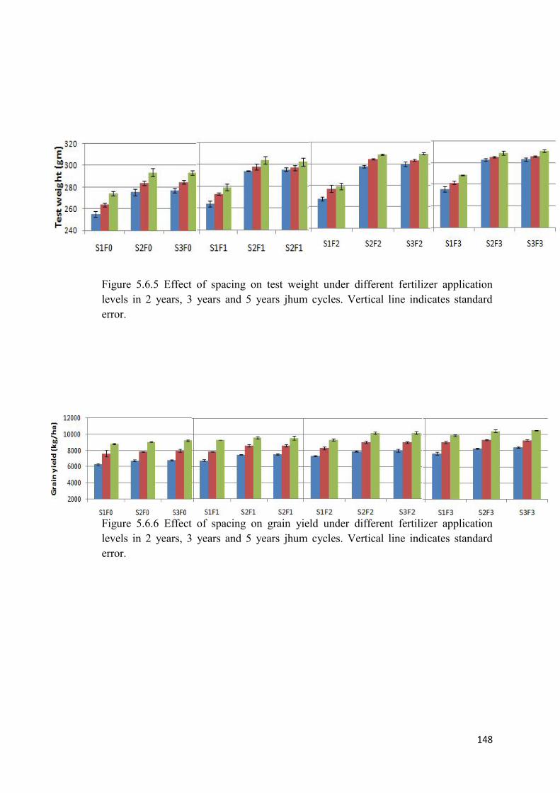
148
Figure 5.6.5 Effect of spacing on test weight under different fertilizer applicationlevels in 2 years, 3 years and 5 years jhum cycles. Vertical line indicates standarderror.
Figure 5.6.6 Effect of spacing on grain yield under different fertilizer applicationlevels in 2 years, 3 years and 5 years jhum cycles. Vertical line indicates standarderror.

149
Table5.6.5: Effect of spacing on Test weight (1000 grain wt.) under different levels offertilizer application levels in 2, 3 and 5 years jhum cycles. Mean ±SEM
* = P<0.05, ** = P<0.01, *** = P<0.001
Table 5.6.6: Effect of spacing on grain yield under different levels of fertilizerapplication in 2, 3 and 5 years jhum cycles. Mean ±SEM.
* = P<0.05, ** = P<0.01, *** = P<0.001
S1F0 S2F0 S3F0LSD(0.05) S1F1 S2F1 S3F1
LSD(0.05) S1F2 S2F2 S3F2
LSD(0.05) S1F3 S2F3 S3F3
LSD(0.05)
2JC 255.33±2.60
275.33±3.18
277.00±2.08
**20
264.33±2.40
294.33±0.33
295.59±1.75
***30
267.46±1.86
297.67±1.45
300.00±2.08
***30.20
275.67±2.40
303.00±1.16
303.28±1.36
***27.33
3JC 263.67±1.86
283.67±1.86
284.67±1.45
***20
273.33±1.20
298.14±2.59
297.33±2.33
***24
277.00±3.22
304.33±0.67
303.67±0.88
***26.66
281.67±1.45
305.33±0.88
306.00±0.58
***23.66
5JC 274.20±1.73
293.50±3.67
293.33±2.19
**19.13
279.38±2.91
304.05±3.47
302.67±3.84
**23.28
279.33±3.18
309.00±0.58
309.67±0.88
***29.66
288.73±0.37
309.24±1.92
311.08±1.45
***20.51
S1F0 S2F0 S3F0LSD(0.05) S1F1 S2F1 S3F1
LSD(0.05) S1F2 S2F2 S3F2
LSD(0.05) S1F3 S2F3 S3F3
LSD(0.05)
2JC 6274.4±105.1
6764.2±127.3
6813.0±77.7
*489.82
6790.9±93.1
7509.7±37.5
7551.4±75.2
***718.71
7333.9±79.2
7924.2±87.5
8022.5±184.0
*590.29
7683.5±188.9
8294.8±46.2
8449.9±64.6
**611.28
3JC 7614.7±388.8
7842.8±38.1
7983.1±149.8 ns
7903.9±44.1
8636.0±155.8
8636.3±159.3
*732.13
8337.8±178.2
9047.9±149.5
9048.3±99.7
*710.10
9057.8±145.2
9368.0±64.9
9317.7±93.2 ns
5JC 8806.8±76.8
9051.7±30.2
9219.5±85.7
*244.91
9347.2±29.4
9622.1±149.5
9586.9±238.6 ns
9325.0±148.9
10177.6±155.5
10216.8±165.0
*852.53
9919.9±103.9
10435.0±171.5
10549.9±40.3
*515.07

150
Figure 5.6.7 Effect of spacing on harvest index under different fertilizer applicationlevels in 2 years, 3 years and 5 years jhum cycles. Vertical line indicates standarderror.
Table 5.6.7: Effect of spacing on Harvest Index (HI) under different levels fertilizerapplication in 2, 3 and 5 years jhum cycles. Mean ±SEM
* = P<0.05, ** = P<0.01, *** = P<0.001
S1F0 S2F0 S3F0LSD(0.05) S1F1 S2F1 S3F1
LSD(0.05) S1F2 S2F2 S3F2
LSD(0.05) S1F3 S2F3 S3F3
LSD(0.05)
2JC 0.262±0.011
0.320±0.019
0.323±0.007
*0.05
0.256±0.006
0.341±0.008
0.326±0.002
***0.07
0.259±0.004
0.332±0.002
0.335±0.010
***0.07
0.265±0.008
0.335±0.007
0.339±0.006
***0.07
3JC 0.313±0.011
0.381±0.007
0.375±0.006
**0.06
0.289±0.004
0.385±0.009
0.370±0.007
***0.08
0.290±0.007
0.371±0.008
0.370±0.005
***0.07
0.309±0.011
0.374±0.008
0.371±0.006
**0.06
5JC 0.350±0.009
0.405±0.004
0.408±0.008
**0.05
0.325±0.006
0.391±0.005
0.385±0.011
**0.06
0.328±0.010
0.400±0.006
0.406±0.005
***0.07
0.348±0.006
0.405±0.007
0.405±0.006
**0.06

151
Chapter – VI
Discussion
6.1 Effect of NPK fertilizer on growth performance
6.1.1 Effect of fertilizer applications on plant height
The sowing of seeds on 24 March coincided with the summer rain
resulted in the early germination of seeds. The significant difference in height among
the fertilizer different levels of fertilizer application with better plant height under
higher rate of fertilizer application may be due to the improvement of seedling vigor
by the availability of soil nutrients for the developing seedlings. Improvement of
seedling vigor is necessary for the survival and yield of crops plants. The minimum
height in plots without fertilizer application and the increasing in plant height with
increasing in fertilizer application indicated the early response of maize seedlings to
soil nutrient availability. The non significant difference in plant height among the
jhum cycles in most of the fertilizer levels indicated the low response to different
jhum cycles a the initial stage of growth.
The plant height under different fertilizer levels at 30DAS exhibited a
marked shift from that of the plant height at 15DAS as highly significant difference
occurred among the jhum cycles. Less significant variations among the fertilizer plots
in each of the spacings may be due to depletion of soil nutrients due to leaching by
rainfall and that the highly significant difference among the jhum cycles may be
attributed to the different natural soil condition among the jhum cycles.
The increase in the significant level from that of 30DAS in plant height
of maize under different fertilizer levels may be due to response of plants to the
second dose of NPK fertilizer which was applied at 30DAS. The higher percentage

152
increase from the minimum height to the maximum height in 2JC and 3JC may be due
to the high influence of nutrient application in these two jhum sites of poorer soil
nutrient properties than the 5JC. High growth rate in height during the period of 30 to
45DAS coincided with the increasing in rainfall which enhances growth performance.
Compared to 2JC and 3JC, higher growth rate was observed among the plants in the
fertilizer plots of 5JC.
Measurement of plant height at 60DAS showed highest growth rate in
plants under different fertilizer levels in 2JC and 3JC where as reduction is growth
rate was observed in 5JC when compared with that of the growth rate at 45DAS.
Despite of the wide range in plant height between plants of 2JC and 3JC to that of the
corresponding treatment in 5JC in 45DAS, the range become narrower due to the high
growth rate of plants in 2JC and 3JC.
From the observation plant growth performance in terms of height, it is
obvious that soil nutrient deficit is one of the major limiting factors for plant growth
in the different jhum cycles of Mizoram. Fertilizer application and longer jhum cycle
induced vigorous growth during the 15 to 45DAS. Plant height is one of the crucial
factors which determines the survival and productivity of the plant. Higher plant
height has better light interception which facilitates higher photosynthetic rates under
favourable condition. From the observation of highest plant height corresponding with
highest fertilizer application, it might be suggested that increase the levels of NPK
fertilizer application might still enhance the growth performance of the mimpui
variety of maize.
6.1.2 Effect of NPK fertilizer application on number of leaves per plant
The non-significant and low significant variations in number of leaves
per plant in all the fertilizer levels as well as among the jhum cycles indicted that the

153
leaves production was uniform regardless of soil nutrient input and difference in jhum
cycles. Although the highly significant variation in plant height at this growth stage
did not induced much variations in leaves production as all the plants under different
fertilizer application levels as well as jhum cycles showed narrow range in number of
leaves per plant.
As the growth progressed, higher variations among the plants under
different fertilizer applications as well as the jhum cycles indicated that the influence
of soil nutrient availability became more evident. More variations were observed at
45DAS in the number of leaves per plant. Similar trend with that of plant height of
increasing number of leaves with increasing fertilizer application levels as well as the
jhum cycles was still observed at 45DAS.
Despite of the higher significant difference in height at 60DAS, the
number of leaves at 60DAS showed lesser significant levels between fertilizer plots as
well as the jhum cycles. This indicated that the number leaf production was less
affected by fertilizer input and jhum cycles, and the higher variations in plant height
did not necessarily induced greater number of leaves per plant. Thus, the increase in
height might be due to the increase in internode length rather than the production of
more nodes for leaf production.
6.1.3 Effect of NPK fertilizer onpPlant dry biomass
The plant biomass production was also strongly affected by fertilizer
applications. Under the same spacing, the occurrence of lowest biomass production in
plots without fertilizer input and the increase with increase in fertilizer application
levels showed similar trend with that of plant height and number of leaves per plant.
Plant biomass production was comparable between the fertilizer plots of S2 and S3
spacings. The sharp increase in biomass production from F0 towards F2 and the lesser

154
increased between the F2 and F3 plots in S1, S2 and S3 spacing indicated that the
affect of fertilizer on biomass production was more pronounced between F0 to F2 and
further increase from F2 to F3 level had lesser impact on biomass production.
6.2 Effect of NPK fertilizer application on yield parameters
6.2.1 Length of cob
The length of cob which is a important yield parameter was
significantly affected by fertilizer application showing wide range of less
than15.00cm to greater than 19.00 cm in 2JC, 16.00cm to greater than 20.00cm in
3JC and, less than 18.00cm to greater than 22.00cm in 5JC among the spacing and
fertilizer treatment. This implied the strong impact of space and nutrient availability
on growth and the resultant biomass production of maize plant.
6.2.2 Kernel rows per cob
The number of kernel rows per cob is one of the important yield
parameters than determine grain yield in maize. Although increasing trend of kernel
rows per cob was observed from the F0 plot toward F3 plot in all the three spacing,
there was only few significant difference. The inter jhum comparison also showed
significant increase from 2JC toward 5JC in all the fertilizer plots of S1 but less
significant variations in fertilizer plots of S2 and S3.
6.2.3 Kernels per row
Unlike kernel rows per cob, significant increase in the number of
kernel from F0 toward F3 except in S2 spacing of 2JC indicated the strong impact of
NPK fertilizer under different plant spacing. High rate of increased in number of
kernels per row was observed from F0 toward F2 indicating the best response to NPK
fertilizer by maize plant in the F1 and F2 application rate.
155
The highly significant increase in number of kernels per row 2JC to 5JC indicated the
soil condition of longer jhum cycles might induced more kernels per row in maize.
From the uniform increase in kernels per row from 2JC to 5JC, it is suggested that
logner jhum cycles may induce further increase in number of kernels per row.
6.2.4 Kernels per cob
The similar pattern between length of cob and kernels per row of
significant increase in with increase fertilizer levels as well as with the increase in
jhum cycle resulted in the increase in total number of kernels per cob from plot
without fertilizer application toward the highest level of fertilizer application as well
as with the longer jhum cycles. Considering the overall range under different fertilizer
application, spacing and jhum cycles, the wide range of the number of kernels per
cob, it is evident that this was one of the most variable parameters and it could be
crucial determinants of grain yield.
6.2.5 Test weight
The test weight was highly influenced by NPK fertilizer application
under different spacing which indicated that NPK fertilizer induced the improvement
of the quality of the kernel which manifested in the greater weight of 1000 seed
grains. The significant increase in test weight from the 2JC to 5JC was also a strong
determinant of grain yield of maize.
6.2.6 Grain yield/ha
The grain yield per hectare which was extrapolated from the yield per
plant indicated the strong effect of fertilizer on grain yield of maize. Considering the
increased in grain yield from the lowest yield in the highest density spacing (55cm x
20cm) without fertilizer application to the highest fertilizer application (120:60:40
kg/ha of NPK) with wider spacing (60cm x 25cm), the productivity of maize depend

156
strongly on the cultural practice and selection of the most appropriate spacing and
fertilizer input is the prerequisite. The strong influence of jhum cycles also indicated
its impact of the yield of maize.
Although harvest index showed no significant variations among the
fertilizer plots under different spacing, the significant difference among the jhum
cycles indicated the grain yield per gram of biomass produced increases with increase
in jhum cycles.
6.3 Effect of plant spacing on growth performance
6.3.1 Plant height
The effect of spacing on plant height increases with the progressed of
the growth period and at 60DAS, spacing induced significant difference in plant
height. This less significant variations at the early stage of growth was attributed to
the sufficient space for plant at this stage. As the growth progressed more spatial
competition in the high density spacing resulted in the reduction in plant height at S1
spacing of 55cm x 20cm that 90,909 plants per hectare. The S2 and S3 spacing of
75cm x 20cm (66,666 plants/ha) and 60cm x 25cm (66,666 plants/ha) showed
comparable growth rates.
6.3.2 Number of leaves per plant
The effect spacing on the number of leaves per plant also increased
with the increasing growth period with significant variations among the S1, S2 and S3
spacings in all the fertilizer application levels. Number of leaves was greatly reduced
in highest plant density of S1 spacing.
6.3.3 Biomass production
Biomass production was strongly influenced by spacing with great
reduction in plant dry biomass in S1 spacing. At high density planting, plants compete

157
of vertical growth for better light inception which led to production of weak slender
stalk in plants. The greater plant height and number of leaves felicitates high
photosynthetic rates as well as larger photosynthetic area which improves further
growth and development.
6.3.4 Effect of spacing on yield parameters
The S1, S2, and S3 had strong similar impact on length of cob, kernel
rows per cob, kernels per row, kernels per cob and seed test weight which were the
determinants of the grain yield. The S1 spacing of high density planting (90,909
plants/ha) considerable reduce the yield parameters.
The impact of spacing on grain yield was less significant when compared with that of
the effect of fertilizer application.
The harvest index (HI) was strongly affected by spacing with low HI in the highest
density plant of 55cm x 20cm. This implied that despite of the lowest biomass
production in S1 spacing in each of fertilizer plots; the grain yield was proportionately
lower which resulted in lower HI.
158
Chapter VI
SUMMARY AND CONCLUSION
1. The study was carried out at the Edenthar locality which is at the outskirt of
Aizawl city.
2. The jhum cycles viz. 2 years, 3 years and 5 years cycles were selected to study
the extent of the influence of different jhum cycles on growth and productivity
of maize.
3. Most promising local variety of maize called ‘Mimpui” was selected as it has
a high potential for commercial production of corn to meet various demands
for human consumption as well as animal feeds.
4. Maize were grown under four levels of Nitrogen, phosphorus and potassium
fertilizer treatments of 80N:40P:20K, 100N:50P:30K, 120N:60P:40K (NPK
kg/ha) and Control (Without NPK) with combination of three different spacing
of 75cm x 20 cm, 60 cm x 25 cm and 55cm x 20 cm.
5. Local maize variety grown under four levels of fertilizer treatments and two
levels of spacing in three 2 years, 3 years and 5 years jhum cycles showed
significant response in growth performance and yield characteristics
6. The variations in plant height and number of leaves per plant became more
pronounced with the progress in growth period.
7. Fertilizer significant enhanced seedling vigor and plant growth.
8. Spacing also significantly affected plant growth which became more evident
with increase in growth period as the competition for space and nutrient
increases.
159
9. Highly density spacing of 55cm x 20 cm greatly reduce the growth and yield
performance.
10. In most of the growth and yield parameters, lowest values were observed in
plot with highest density and without fertilizer application where as plant
spacing of 60cm x 25 cm showed maximum values in most of the parameters.
11. Jhum cycles significantly influenced growth performance in which poor
growth was observed in shorter jhum cycle of 2 years when compared with 5
years jhum cycles.
12. Yield parameters were highly influenced by fertilizer application which
increased with increase in fertilizer input.
13. Length of cob, number of kernels per row and test weight were the parameters
which strongly influenced the grain yield.
14. Minimum grain yield of 6274.4 kg/ha occurred in highest plant spacing with
no fertilizer application in 2 years jhum cycle.
15. Highest grain yield of 10549.9 kg/ha occurred in the 5 years jhum cycle with
highest level of fertilizer application (120: 80 : 40 NPK per hectare)
16. From this experiment, it is evident that low soil nutrient under frequent jhum
cycles is the major limiting factor for growth and yield of maize in the hilly
slopes of Mizoram.
17. Considering the growth and yield under the three spacing, 60cm x 25cm is
likely to be the most promising.
From this study, considering the overall effect of fertilizer, spacing and
jhum cycles; the increased from the minimum values to the maximum values
accounted for 43% in plant height at 60DAS, 26% in number of leaves at 60DAS,
160
47.79% in biomass per plant, 50% in length of cob, 28.15% in kernel rows per cob,
88% in kernels per cob, 21.83% in seed test weight, 68.14% in grain yield/ha, 54.58%
in harvest index. This strongly indicated that optimization of cultural practice in in
terms of spacing, fertilizer input and jhum cycles is needed for sustainable agriculture
system even under jhum cultivation without compromising the yield of the Mimpui
variety.
Maize is a nutrient demanding crop and due to its high uptake rate of
available nitrogen, phosphorus and potassium from soil, fertilizer application in the
successive cropping season may be prerequisite in similar jhum cycles to supplement
the nutrient removal of the previous crop. Also due to the acidic condition of the soil,
careful monitoring in application of acidic fertilizer like urea needed to be conducted
to prevent setting up of unfavourable soil condition such as aluminium toxicity. From
this experiment, it is observed that the Mimpui is a high yielding variety that could be
promoted for commercial corn production. Considering the strong effect of NPK
fertilizer in grain yield and at the same time the delicate soil condition under jhum
cultivation, it is suggested that 5 years jhum cycle with lower rate of fertilizer
application (80:40:20 NPK kg/ha) with spacing of 60cm x 25cm may be adopted.

161
REFERENCES
Adediran J.A & Banjoko V.A, (1995). Response of maize to nitrogen, phosphorus
and potassium fertilizers in the savanna zones of Nigeria. Communications in
Soil Science and Plant Analysis; (3-4), pp. 593-606.
Adediran, J. A. and. Banjoko V. A, (2003). Comparative effectiveness of some
compost fertilizer formulations for maize in Nigeria. Nig. J. Soil Sci., 13:42-
48.
Adeniyan, O. N., Ojo, A. O., Akinbode, O. A. and Adediran, J. A., (2011).
Comparative study of different organic manures and NPK fertilizer for
improvement of soil chemical properties and dry matter yield of maize in
two different soils. Journal of Soil Science and Environmental
Management. 2(1), pp. 9-13.
Adger, W. N. and Brown, K., (1994). Land Use and the Causes of Global Warming.
New York, John Wiley and Sons. 36: 117-133.
Agrawal, K.N, Singh, R.K.P, Satapathy, K.K, (2010). Anthropometric considerations
for farm tools/machinery design for tribal workers of North Eastern India.
Agricultural Engineering International: the CIGRE journal, Manuscript MES
1406 Vol. XII.
Akinnifesi, F.K, Sileshi, G., Ajayi, O.C., Chirwa, P.W., Mngomba, S., Chakeredza, S.
and Nyoka, B.I. (2008). Domestication and Conservation of Indigenous
Miombo Fruit Trees for Improving Rural Livelihoods in Southern Africa,
Tropical Conservancy, pp. 72-74.
162
Akinrinade, E.A., Iroh l, Obigbesan, G.O., Hilger T., Romheld V., Neumann G.,
(2006). Response of cowpea varieties to phosphorus supply on an acidic
alumi-haplic-Acrisol from Brazil. Nig. J. Soil Sci., 16: 115-120.
Akintoye, (1996). Thesis Abstract, International Institute of Tropical Agri Research,
pp. 25–27.
Alexandratos, N. and Bruinsma, J., (2012). World agriculture towards 2030/2050: the
2012 revision. ESA Working paper No. 12-03. Rome, FAO.
Ali, I.A.N.M., Das, I., (2003). Tribal Situation in North East India. Stud. Tribes
Tribals, 1(2): 141-148.
Altieri, M. A., Anerson, M. K., Merrick, L. C., (1987). Peasant agriculture and the
conservation of crop and wild plant resources. Conservation Biology, 1(1):
49-58.
Amor, D., (2008). Road impact on deforestation and jaguar habitat loss in the Selva
Maya. Ph. D. dissertation. Ecology Department, Nicholas School of the
Environment, Duke University.
Amor, D., and Pfaff, A., (2008). Early history of the impact of road investments on
deforestation in the Mayan forest. Working Paper, Nicholas School of the
Environment and Sanford School of Public Policy, Duke University, Durham,
NC, USA.
Andersen, K.E., Sophorn, S. and Thornberry, F. (2008). Development of a sub-decree
on shifting cultivation under Article 37 of the Forestry Law (2002), Cambodia,
International Labor Organisation, Support to Indigenous People Project in
Cambodia.pp 1-36.

163
Angelsen, A., Shitindi, E. F. K., and Aaarrestad, J., (1999). Why do farmers expand
their land into forests. Theories and evidence from Tanzania. Environment
and Development Economics 4: 313-31.
Angelsen, A., (1999). Agricultural expansion and deforestation: modeling the impact
of population, market forces and property rights. Journal of Development
Economics 58: 185-218.
Anonymous, (1987). Basic statistics for north-eastern region (Shillong: North-Eastern
council).
Anonymous, (1991a). Soils of Mizoram; Drectorate of Agriculture, Mizoram; pp 1-7.
Anonymous, (1992). Agro-climatic planning for agricultural development in
Meghalaya. Working group, Zonal Planning Team, Eastern Himalayan
Region, AAU, Jorhat.
Anonymous, (1994a). Deforestation Technical Support Package. Third International
Conference on Environment Enforcement, Oaxaca Mexico April 25- 28, 1994.
World Wildlife Fund; U. S. Environmental Protection Agency and U. S.
Agency for International Development.
Anonymous, (1996). Data on expenditure under NLUP in Mizoram. Rural
Development Department, Government of Mizoram, Aizawl, Mizoram,
India.
Anonymous, (2000). Wastelands Atlas of India, Ministry of Rural Development,
Government of India and National Remote Sensing Agency,
Hyderabad, India.
Anonymous, (2001). State of Forest Report, Forest Survey of India. Ministry of
Environment and Forests, Government of India.
164
Anonymous (2002). Forest certification and biodiversity: opposites or complements.
Discussion paper prepared for the GEF, International Tropical Timber
Organization, Yokohama Japan.
Anonymous, (2003). Mizoram Forest. Department of Environment and Forest, Govt.
of Mizoram. pp 1-15.
Anonymous, (2004a). Statistical Handbook of Mizoram. Directorate of Economic
and Statistics, Govt. of Mizoram, pp 1-9.
Anonymous, (2004b). Statistical Abstract. Dept. of Agriculture and Minor irrigation,
Mizoram. pp 1-3, 42-43.
Anonymous, (2005). Ecosystems and Human well-being: synthesis. Millennium
ecosystem Assessment. Island Press, Washington DC.
Anonymous, (2006). Statisical Hand Book of Mizoram, 2006. Directorate of
Economics & Statistics, Ail, Mizoram, India. pp. 5 and 106.
Anonymous, (2008a). Statistical Hand Book. Dirctorate of Economics & Statistics,
Mizoram; Aizawl. pp 145.
Anonymous, (2009). Draft report of the inter-ministerial national task force on
rehabilitation of shifting cultivation land. Report submitted to the Ministry of
Environment and Forests, Government of India, pp. 1-25.
Anonymous, (2010). Global Forest Resources Assessment, 2010-Main Report. FAO
Forestry Paper 163. Rome, Italy. pp-340.
Anonymous, (2011). India achieves 241 MT foodgrain production in 2010-11: PM.
http://businesstoday.intoday.in/story/foodgrain-production-in-india-2010-11-
pm/1/17062.html.
165
Anonymous, (2011). Regional project implementation plan. North East rural project,
Ministry of DONER, Govt. of India. http://sirdmizoram.org/.
Anonymous, (2011). The Meteorological data of Mizoram. Department of Economics
and Statistics Mizoram, Aizawl. pp 17.
Arunachalam. A., Khan, M.L., Arunachalam, K., (2002). Balancing Traditional jhum
cultivation with modern agroforestry in Eastern Himalaya- A biodiversity
hotspot. Current Science, 83(2): 117-118.
Awotundun, J.S., (2005). Comparative Effects of organic and inorganic fertilizer on
the yield of pop-corn. In: Proceedings of the 29th Annual Conference of the
Soil science society of Nigeria. December, 6th-10th, 2004. University of
Agriculture Abeokuta, Nigeria. Pp. 175-179.
Azam, S., Ali, M., Amin, M., Bibi, S. and Arif, M., (2007). Effect of plant population
on maize hybrids. Journal of Agricultural and Biological Science. 2(1): 13-20.
Azeez, J.O., Adetunji, M.T, and Adetunji, B., (2007). Effects of Residue burning and
Fertilizer application on soil Nutrient dynamics and dry grain yield of maize
(Zea mays L.) in an Alfisols. Nigerian Journal of Soil Science. 7: 71-80.
Bam, M., (2015). “Jhum cultivation practices of the Galo of Arunachal Pradesh.
International Journal of current Research, 7 (9): 20325- 20329.
Banziger, M., Edmeades, G. O., Beck, D. and Bellon, M., (2000). Breeding for
Drought and Nitrogen Stress Tolerance in Maize. From Theory to Practice.
CIMMYT, Mexico, pp68.
Baran, M., (1987). Effect of Nitrogen Application on the Production and Nutritive
Value of Maize and Soya Bean Mixture. Polnohespodarstov, 37: 613-624.

166
Barah, B.C., (2007). Strategies for Agricultural Development in the North-East
India: Challenges and Emerging Opportunities. Ind. Jn. of Agri. Econ.
62(1): 1-31
Barber, S.A., (1995) Soil Nutrient Bioavailability: A Mechanistic Approach, 2nd Ed.
John Wiley & Sons, New York. Pp- 414.
Barbier, E.B., (2000). Links between economic liberalization and rural resource
degradation in the developing regions. Agricultural Economics, 23(3), pp.
299-310.
Bationo, A. and. Lompo, F., (2003). Available technologies for combating soil
Nutrients losses in West Africa. In: Gichuru, M.P., A. Bationo, M.A.
Bekunda, H.C. Goma, P.K.Mafungoya, D.N. Mugendi and H.J. Swift (Eds).
Soil fertility management.for Sustainable Land use in the West. pp. 31-48.
Begna, S.H., Hamilton, R.I., Dwyer, L.M., Steward, D.W., Smith, D.L., (1997).
Effects of population density and planting pattern on the yield and yield
components of leafy reducedstature maize in a short-season area, J.
Agronomy & Crop Science, 179, pp. 9-17.
Biggelaar, D. C., Lal, R., Wiebe, K., Breneman, V., Reich, P., (2004). The global
impact of soil erosion on productivity II: effects on crop yields and production
over time. Adv Agron 81: 49-95.
Bormann, F.H., Likens G.E., (1980). Pattern and Process in a Forested Ecosystem,
Folia Geobotanica & Phytotaxonomica, 15(4): 426-428.
Borthakur, D. N., Singh, A., Awasthi, R. P. and Rai, R. N.,(1978). Shifting
cultivation in the northeastern region. In Proceedings of the National Seminar
on Resources, Development and Environment in the Himalayan Region, DST,
New Delhi, pp. 330–342.

167
Borthakur, D.N., Prasad, R.N., Ghosh, S.P., Singh, A., Awasthi, R.P., Rai, R.N.,
Varma, A., Datta, H.H., Sachan, J.N. and Singh, M.D. (1979). Agro forestry
based farming system as an alternative to Jhuming. Reprinted from Seminar
Proceedings on Agro-forestry organised by ICAR at Imphal, Manipur, Pp. 32p
Borthakur, D.N., (1992). Agriculture of the North Eastern Region with Special
Reference to Hill Agriculture, Bee cee Prakashan, Guwahati, India. Pp. 637.
Boucher, D., Roquemore, S. and Fitzhugh, E., (2013). Brazil’s success in
reducingdeforestation. Tropical Conservation Science. 6(3):426-445.
www.tropicalconservationscience.org
Brady, N.C., (1984). The nature and properties of Soils. Macmillan Publishing
Company, New York, Pp. 152-158 .
Brighter Green & G.F.C., (2013). Livestock Farming, Communities, Biodiversity and
Climate Change - 2013/10/FINAL-version-livestockbriefing-Oct-ENG.
Pp.1-10.
Brown, L., (1994). Facing food insecurity, A Worldwatch Institute Report on Progress
Toward a Sustainable Society. In: L. Brown (ed.), The State of the World.
New York, NY, W.W. Norton & Co. Chapter 10.Pp. 274.
Bundy, L G., Andraski, T. W., Wolkowski, R. P., (1993). Nitrogen credits in
soybean-corn corps: sequences on three soils. Agron. J. 85: 1061-1067.
Carr, D., Sutter, L., Barbieri, A., (2006). “Population Dynamics and Tropical
Deforestation: State of the Debate and Conceptual Challenges.” Population
and Environment 27:89-113.
Chhakchhuak, L., (2004). Jhum Works, Shillong Declares on Jhum: Benefits Jhum
cultivation. Down to earth, 15th Nov. 2004.

168
Chomitz, K.M., Buys, P., Luca, G.D., Thomas, T.S., Wertz-Kanounnikoff, S.,
(2007). At loggerheads. Agricultural expansion, poverty reduction, and
environment in the tropical forests. Washington, DC: The World Bank.
Clergeau, P., Savard, J.P.L., Mennechez, G., Falardeau, G., (1998). Bird abundance
and diversity along an urban-rural gradient: A comparative study between
two cities on different continents, Condor, 100: 413–425.
Colchester, M., and Lohmann L., (1993). The Struggle for land and the fate of forest.
The Ecologist, Sturminster Newton and Zed Books Ltd, London. Pp. 389.
Conklin, H. C.(1961). The study of shifting cultivation. Current Anthropology, 2(1),
pp. 27-61.
Cossalter, C. and Pye-Smith, C., (2003). Fast-wood forestry, myths and realities.
Forest Perspectives no. 1, CIFOR, Bogor Indonesia. Pp.54.
DOI: 10.17528/cifor/001257
Cramb, R.A. et al., (2009). Swidden Transformations and Rural Livelihoods in
Southeast Asia. Human Ecology 37: 323-346
Das, E.S., Choudhury, E.S., Roy, A.A., (2012). The Success Story of Rehabilitation
of Jhumias in Tripura- A Study on Baramura-Deutamura Range. International
Journal of Engineering and Science,1(10): 25-29.
Dale and Virginia, H., (1997). The relationship between land-use change and climate
change. Ecological Applications, 7 (3): 753-769.
Deka and Sarmah, D., (2010). Shifting cultivation and its effects in regarding of
perspective in Northern India. International Journal of Commerce and
Business Management, 3(2) : 157-165.
169
Devi, N.L. and. Choudhury, B.U., (2013). Soil fertility status in relation to fallow
cycles and landuse practices in shifting cultivated areas of Chandel district
Manipur, India. Journal of Agriculture and Veterinary Science; 4(4): 01-09.
Dewangan, K.N., Prasanna Kumar, G.V., Datta, R.K., (2004). Scope of
mechanization in Arunachal Pradesh, PartII: present status and future
strategies. Agric. Eng. Today 28 (5-6): 44-51.
Dewangan, K.N., Owary, C., Datta, R.K., (2010). Anthropometry of male
agricultural workers of north-eastern India and its use in design of agricultural
tools and equipment. International Journal of Industrial Ergonomics 40(5):
560-573.
D.I.P.A., (2006). Handbook of Agriculture: facts and figures for farmers, students and
all interested in farming. Directorate of Information and Publications of
Agriculture. Indian Council of Agricultural Research, New Delhi,pp. 435.
Dobermann, A. and Nelson, R., (2013). Opportunities and Solutions for Sustainable
Food Production. Background paper for the High-Level Panel of Eminent
Persons on the Post-2015. Pp.1- 11.
Duncan W.G., (1980). Maize L.T. Evans (Ed.), Crop Physiology, Cambridge Univ.
Press, pp. 23–50.
Dwivedi, A.P., (2001). Agroforestry Principles and Practices, (Oxford & IBH
Publishing Company Private Limited, New Delhi), pp- 365.
Eden, M.J., Andrade, A., (1987). Ecological aspects of swidden cultivation among the
Andoke and Witoto Indians of the Colombian Amazon. Human Ecology,
15(3): 339-359.
170
Egger, K., (1981). Ecofarming in the tropics – characteristics and potentialities. Plant
Research and Development, 13(1): 96-106.
El Noeman, A. A., El-Halem, A.K.A., El-Zeiny, H.A., (1990). Response of maize
(Zea mays L.) to irrigation intervals under different levels of nitrogen
fertilization. Egyptian J. Agron., 15 (1–2): 147–158.
Enujeke, E. C., (2013). Response of Grain Weight of Maize to Variety, Organic
Manure and Inorganic Fertilizer in Asaba Area of Delta State. Asian Journal
of Agriculture and Rural Development, 3(5): 234-248.
Enwezor, W.O., Udo, E.J., Sobulo, R.A., (1981). Fertility status and productivity of
the ‘Acid Sands’. In, Udo, EJ. and Sobulo, RA. ‘Acid Sands’ of Southern
Nigeria. (1): 56-53.
FAO, (2002). Fertilizer and the future. IFA/FAO Agriculture Conference on Global
security and the role of Sustainability Fertilization. Rome, Italy. pp 1-2.
FAO, (2006). The State of Food Insecurity in the World. Eradicating world hunger –
taking stock ten years after the World Food Summit. Rome.
Farnham, D.E., Benson, G.O., Pearce, R.B., (2003). Corn perspective and culture.
Chapter 1. In:PJ White, L.A Johnson,eds. Corn: Chemistry and technology,
Edition 2nd. American Association of Cerial Chemicals, Inc. St. Paul,
Minesota, USA. pp1-33.
Fashina, A. S., Olatunji, K.A and Alasiri, K.O., (2002). Effects of different plant
population and poultry manure on yield of Ugu (Telfairia occidentalis) in
Lagos State, Nigeria in Proceedings of the annual Conference of Horticultural
Society of Nigeria (HORTON), pp. 123-127.
171
Fearnside P.M and Barbosa R.I, (1998). Soil carbon changes from conversion of
forest to pasture in Brazilian Amazonia. Forest Ecology and Management,
108 (1-2): 147-166.
Fischer, G., Shah, M., Tubiello, F.N & Velhuizen, H.V., (2005). Socio-economic and
climate change impacts on agriculture: an integrated assessment, 1990-2080.
Philosophical Transactions of the Royal Society ,B.360: 2067-2083.
FPDD, (2002). Fertilizer use and Management Practices for Crops in Nigeria. The
Fertilizer Procurement and Distribution Division of the Federal Ministry of
Agriculture, Water Resources and Rural Development, Abuja, pp 1-20.
Gasim, S.H., (2001). Effect of nitrogen, phosphorus and seed rate on growth, yield
and quality of forage maize (Zea mays L.). M.Sc. Thesis, Faculty of Agric.,
Univ. of Khartoum.
Galloway, J., Burke, M., Bradford, E., Naylor, R., Falcon, W., Chapagain, A.K.,
Gaskell, J., McCullough, E., Mooney, H., Oleson, K., Steinfeld, H.,
Wassenaar, T., Smil, V., (2007). International Trade in Meat: The tip of the
pork. Ambio : A Journal of the Human Environment, 36(8):622-629.
Geist, H., and Lambin, E., (2002). Proximate causes and underlying driving forces of
tropical deforestation. BioScience 52: 143-150
Giller, K., and Palm, C., (2004). Cropping systems: Slash-and burn cropping systems
of the tropics. Encyclopedia of Plant and Crop Science. pp 363-366.
Goswami, P.C., (1968). Shifting Cultivation and its Control in the Garo Hills, (Soil
Conservation Department of Assam).

172
Gong, W., Xiaoyuan Yan X., Jingyan Wang J., (2011). The effect of chemical
fertilizer on soil organic carbon renewal and CO2 emission a pot
experiment with maize. Plant and Soil, 353(1): 85-94.
Government of India (GOI), 2000. Guidelines for watershed development project in
shifting cultivation areas. Ministry of Agriculture, New Delhi.
Green, C.J., Blackmer, A.M., (1995). Residue decomposition effects on nitrogen
availability to corn flowing corn or soybean. Soil Sci. Am. J. 59: 1065-1070.
Grogan, P., Lalnunmawia, F., Tripati, S.K., (2012). Shifting cultivation in steeply
sloped regions: a review of management options and research priorities for
Mizoram state, Northeast India. Agroforest Syst, 84: 163-177.
Gupta, V., (2005). Jhum cultivation practices of the Bangnis (Nishis) of Arunachal
Pradesh. Indian Journal of Traditional Knowledge. 4(1): 47-56.
Haque, M.M., Hamid, A. and Bhuiyan, N.I., (2001) Nutrient Uptake and Productivity
as Affected by Nitrogen and Potassium Application Levels in Maize/Sweet
Potato Intercropping System. Korean Journal of Crop Science, 46: 1-5.
Harris, D. R., (1971). The ecology of swidden cultivation in the upper Orinoco rain
forest, Venezuela. The Geographical Review, 61(4): 475-495.
Havlin, J.L., Beaton, J.D., Tisdale, S.L. and Nelson, W.L. ( 2005). Soil fertility and
fertilizers: An introduction to nutrient management (7th ed.). Prentice Hall,
Upper Saddle River, NJ. Pp. 515.
Hiraoka, M., Yamamota, S., (1980). Agricultural development in the upper Amazon
of Ecuador. Geographical Review, 70(4): 423-445.

173
Humphreys, D., (2006). Forest Politics. Earthscan Publications Ltd., London. Pp. 302
IAASTD, National Academies of Science (NAS), (2010). Toward Sustainable
Agricultural Systems in the 21st Century. National Academies Press, 500Fifth Street, N.W., Lockbox 285, Washington DC 20055;http://www.nap.edu.ICAR, (1983). Shifting cultivation North east India. Publication unit, ICAR, New
Delhi, pp - 68.
Idso, C.D., (2011). Estimates of Global Food Production in the year 2050. Centre for
the Study of Carbon Dioxide and Global change. www.co2science.org.
Pp.36-43.
IPCC, 2007: Climate Change 2007: Impacts, Adaptation and Vulnerability.
Contribution of Working Group II to the Fourth Assessment Report of the
Intergovernmental Panel on Climate Change, M.L. Parry, O.F. Canziani, J.P.
Palutikof, P.J. van der Linden and C.E. Hanson, Eds., Cambridge University
Press, Cambridge, UK, 976pp.
Jefferson, F., (2009). Policies, Political-Economy, and Swidden in Southeast Asia.
Human Ecology 37: 305-322
Jha, S.D., (1998). Socio economic and demographic dimensions of Arunachal
Pradesh. (Omsons Publications, Guwahati).Pp- 23.
Johnson, Rebecca L. and Chenje, M., (2008). Africa: Atlas of our Changing
Environment (Nairobi, Kenya: United Nations Environment Programme
(UNEP).

174
Kagbe, J.O.S., Adriran, J.A., (2003). Influence of nitrogen, phosphorus and
potassium application on the yield of maize in the savanna zone of Nigeria.
African J. Bio. 2: 345-349.
Kaimowitz, D. and Angelsen, A., (1998). Economic models of tropical deforestation.
A review. Center for International Forestry Research, Bogor Indonesia. CABI
Publishing, CAB International Wallingford Oxon OX10 8DE, UK.
http://www.cabi.org
Kalifa, M.A., Shokr, E.S., Abdella, R.M., Ismail, A.A., (1981). Effect of time of
nitrogen application on an open-pollinated variety of corn (Zea mays L.). Ann.
Agric. Sci.,15, pp. 23–30.
Kartodihardjo, H., Supriono, A., (2000). The Impact of sectoral development on
natural forest conversion and degradation: the case of timber and tree crop
plantations in Indonesia . CIFOR Occasional Paper No.26(E). Bogor,
Indonesia, CIFOR. 14p.
Karmakar, K.G., 2008. Agriculture and rural development in north-eastern India: The
role of NABARD. ASCI Journal of Management 37(2): 89-108.
Katherine, W., (1991). Shifting cultivators – local technical knowledge and natural
resource management in the humid tropics, community Forestry Note 8, FAO
of the UN, Rome.
Keitzer, S., (2001). Technological options for sustainable agriculture in shifting
cultivation areas with special reference to Nagaland. Paper presented in
workshop on sustainable agriculture in shifting cultivation areas. 5-7
February, NIRD-NERC, Guwahati, India.

175
Kellman, M., Miyanishi, K and Hiebert, P., (1985). “Nutrient retention by savanna
ecosystems II. Retention after fire,” Journal of Ecology, 73(3): 953–962.
Khan, A., Munsif, F., Akhtar, K., Afridi, M., Ahmad, Z., Fahad, S., Ullah, R., Khan,
F. and Din, M., (2014). Response of Fodder Maize to Various Levels of
Nitrogen and Phosphorus. American Journal of Plant Sciences, 5: 2323-2329.
http://dx.doi.org/10.4236/ajps.2014.515246
Kisinyo, P.O., Opala, P.A., Palapala, V., Gudu, S.O., Othieno, C.O and Ouma, E.,
(2015). Micro-Dosing of Lime, Phosphorus and Nitrogen Fertilizers Effect on
Maize Performance on an Acid Soil. Sustainable Agriculture Research,
4(2): 21.
Kleiman, P. J., Pimentel, D., Bryant, R. B., (1995). The ecological sustainability of
slash-and-burn agriculture. Agriculture, Ecosystems & Environment,
52(2-3): 235-249.
Koli, S. E., (1971). Effects of spacing and fertilizer on growth and yield of maize.
Ghana Journal of agric. Sci. 4:145-151
Koul, G.G., (1997). Effect of sowing methods, nitrogen levels and seed rates on yield
and quality of fodder maize (Zea mays L.). M.Sc. Thesis, Univ. of Khartoum,
Faculty of Agric, Sudan.
Krall, J.M., H.A., Esechie, R.J., Raney, S., Clark, G., TenEyck, M., Lundquist, N.E.,
Humburg, L.S., Axthelm, A.D., Dayton and Vanderlip, R.L., (1977). Influence
of within-row variability in plant spacing on corn grain yield. Agron. J.,
69:797–799

176
Kushwaha, C.P., Tripathi, S.K., Singh, K.P., (2000). Variations in soil microbial
biomass and N availability due to residue and tillage management in a dryland
rice agroecosystems. Soil Tillage Res. 56 (3-4): 153-166.
Kushwaha, C.P., Tripathi, S.K., Singh, K.P., (2001). Soil organic matter and water
stable aggregates under different tillage and residue conditions in a dryland
agroecosystem. Appl. Soil Ecol., 16(3): 229-241.
Lalnunmawia, F and Tripathi, S.R., (2015). Management of soil fertility and sustained
crop productivity in rice-based agro-ecosystems in Mizoram. Research
Journal of Agriculture and Environmental Management. 4(2):. 088-096.
Latif, A., Alam, S.M., Zafar, I. and Hamid, A., (1992). Effect of rate, time and
method of application of P fertilizer on wheat crop. Proceedings of the 4th
National Congress of Soil Science, Islamabad, pp.299-303.
Lauer, J.G. and Rankin, M., (2004). Corn response to within row plant spacing
variation. Agron. J. 96: 1464-1468.
Law-Ogbomo, K. E. and Law-Ogbomo J.E., (2009). The Performance of Zea mays as
Influenced by NPK Fertilizer Application. Not Sci Biol 1(1): 59-62.
Lele, N., Joshi, P.K., Agrawal, S.P., (2008). Assessing forest fragmentation in
northeastern region (NER) of India using landscape matrices. Ecological
Indicators 8(5): 657-663.
Liang yi, Qi Hua, Wang Jing-ya., (2009). Effects of Growth and Yield of Maize
Under Wide and narrow Row Cultivation. Journal of Maize Sciences.
Tsinghua Tongfang Knowledge Network Technology Co.,
Ltd.(Beijing)(TTKN).
177
Liu, W., Tollenaar, M., Stewart, G. and Deen, W., (2004). Within-row plant spacing
does not affect corn yield. Agron. J. 96: 275-280.
Li yan-ming, Duan wei-wei, Li hui-ling, Xiao kai, (2007). Effects of Density on
Photosynthetic Physiological Characteristics and Yield of Maize. Journal of
Maize Sciences. CateGory Index: S513
Li Ning, Zhai zhi- xi, LI Jian-min, Wu Pei-bo, (2008). Effects of Planting Density on
Agricultural Characters,Root System Characters and Yield of Different Maize
Plant Types. Journal of Maize Sciences. CateGory Index: S513
Li, S.X., Wang, Z.H., Miao, Y.F. and Li, S.Q., (2014). Soil Organic Nitrogen and Its
Contribution to Crop Production. Journal of Integrative Agriculture, (13):
2061-2080.
Lipton, M., and Longhurst, R., (1989). New Seeds and Poor People,: Unwin and
Hyman, London. Pp- 471.
Lombin, L. G., Adeputu, J. A. and Ayetade, K. A., (1991). Complementary use of
organic manures and inorganic fertilizers in arable crop production.
Proceeding of National organic fertilizer seminar, Ibadan. Pp 146 -162.
Lynch, J.P., (2013). Steep, Cheap and Deep: An Ideotype to Optimize Water and N
Acquisition by Maize Root Systems. Annals of Botany, 112: 347-357.
Mandal, R.K., (2011). Changing agricultural scenario and its impact on food habit in
north east states of India. Food Biology, 1(1): 14-21.
178
Mantel, S., Mohiuddin, M., Alam, M.K., Olarieta, J.R., Alam, M., Khan, F.M.A.,
(2006). Improving the jhum system in Bangladesh. Leisa - Magazine on low
external input and sustainable agriculture, 22(4): 20-21.
Marschner H (1995). The soil root interface (rhizosphere) in relation to mineral
nutrition. In: Mineral nutrition of higher plants. 2nd ed. New York (USA):
Academic Press Inc. 537-594.
Marschner, H., (2011) Marschner’s Mineral Nutrition of Higher Plants 3rd Edition.
Elsevier, London. Academic Press, Pp- 672.
Masood, T., Gul, R., Munsif, F., Jalal, F., Hussain, Z., Noreen, N., Khan, H., Din, N.
and Khan, H., (2011). Effect of Different Phosphorus Levels on the Yield and
Yield Components of Maize. Journal of Agriculture, 27, 167- 170.
Mba, C.N., (2006). Influence of organic wastes on plant growth parameters and
nutrient uptake by maize (Zea mays L). Nig. J. Soil Sci., 16: 104-108.
McGrath, D. G.,(1987). The role of biomass in shifting cultivation. Human Ecology,
15(2): 221-242.
Mc Neely, J. and Scherr, S., (2002). Reconciling Agriculture and Biodiversity:
Policy and Research Challenges of ‘Ecoagriculture; World Summit on
Sustainable Development, International Institute for Environment and
Development. Pp. 1-4.
MEA, (2005). Millenium Ecosystems Assessment. Ecosystems and Human Well-
Being. Current State and Trends. Washington. 1: 123-142.
Memon, S.Q., Mirjat, M.S., Mughal, A.Q., Nadeem Amjad, N., Azhar Saeed, M.A.,
Kalwar, S., Mirani, A. L., and Javed, H.I., (2013). Tillage and NPK effect on

179
growth and yield of spring maize in Islamabad, Pakistan. Pakistan J. Agric.
Res. 26(1).
Mertz, O., (2002). The relationship between length of fallow and crop yields in
shifting cultivation: a rethinking. Agroforestry Systems, 55(2):149-159.
Mehra, R., and Rojas M.H., (2008). Women, food security and agriculture in a global
marketplace. Washington, DC: International Center for Research on Women.
Mertz, O., (2009). Trends in shifting cultivation and the REDD mechanism. Current
Opinion in Environmental Sustainability 1:156-160.
Mertz, O., Padoch, C., Fox, J., Cramb, R. A., Leisz, S. J., Lam, N. I., Vein, T. D.,
(2009). Swidden change in Southeast Asia: understanding causes and
consequences. Human Ecology, 37(3): 259-264.
Mikusinski, G., Angelstam, P., (1998). Economic geography, forest distribution, and
woodpecker diversity in central Europe, Conservation Biology, 12: 200–208.
Mishra, A.K., Sharma, U.C., (2001). Traditional wisdom in range management for
resource and environment conservation in northeastern region of India. ENVIS
Bulletin: Himalayan Ecology & Development, 9(1).
Mishra, A.K., Misra, J.P., (2006). Sustainable Development of Agriculture in
Northeastern India: A Quest for More Economical and Resourceful
Sustainable Alternatives. ENVIS Bulletin, Himalayan Ecology, 14 (2): 4-14.
Mitlin, D., (2005). Understanding chronic poverty in urban areas. International
Planning Studies 10(1): 3-19.
Mondal, P., Basu, M., (2009). Adoption of PA Technologies in India and Some
Developing Countries: Scope, Present Status and Strategies. Prog. Nat. Sci.,
19: 659-666.
180
Mona E. El-Azab, (2015). Increasing Zn ratio in a compound foliar NPK fertilizer in
relation to growth, yield and quality of corn plan. JIPBS, Vol 2 (4): 451-468.
Mondal, P., Basu, M., Bhadoria, P.B.S., (2011). Critical Review of Precision Ag
ricultureTechnologies and Its Scope of Adoption in India. Am. J. Exp. Agric.
1(3): 4968.
Munasinghe, M., and Swart, R., (2005). Primer on Climate Change & Sustainable
Development. (CUP, Cambridge, UK).
Muranyi, E., (2015). Effect of plant density and row spacing on maize (Zea mays L.)
grain yield in different crop year. Columella - Journal of Agricultural and
Environmental Sciences, 2(1).
Muldoon, J.F., and T.B. Daynard., (1981). Effects of within-row plant population
variations uniformity on grain yield of maize. Can. J. Plant Sci. 61:887–894.
Myers, N., (1994). Tropical deforestation: rates and patterns. In: The Causes of
Tropical of Tropical Deforestation. The economic and statistical analysis of
factors
National Intelligence Council, (2008). Global Trends 2025: A Transformed World.
United States Office of the Director of National Intelligence: Washington D.C.
Obi, I.U., (1991). Maize, its agronomy, diseases, pests and food values. Optional
Computer Solutions Ltd., Enugu, pp 207.
Obi, C.O., Nnabude, P.C., and Onucha E., (2005). Effects of kitchen waste compost
and tillage on soil chemical properties and yield of Okra (Abelmuschus
esculentus), Soil Sci., 15:6976.

181
OECD, (2011). A Green Growth Strategy For Food And Agriculture. Paris: OECD,
Pp. 19-33.
Onwueme, I.C. and Sinha, T.D., (1991). Field crop production in tropical Africa.
Technical centre for Agriculture and Rural Cooperation pp. 159-175.
Ojima, D.S., Schimel, D.S., Parton, W.J., Owensby, C.E., (1994). Long- and short-
term effects of fire on nitrogen cycling in tallgrass prairie.
Biogeochemistry, 24 (2): 67-84.
Omara, H.A., (1989). The effect of spacing, nitrogen and phosphorus application on
growth and yield of maize (Zea mays L.). M.Sc. Thesis, Univ. of Khartoum,
Faculty of Agric.
Onwueme, I.C. and Sinha T.D., (1991). Field Crop Production in Tropical Africa
CTA. Ede. The Netherlands pp. 159 – 175.
Ortiz, D.M., Apaolaza, L.H., and Gárate A., (2009). Efficiency of a NPK Fertilizer
with Adhered Zinc Lignosulfonate as a Zinc Source for Maize (Zea mays L.).
J. Agric. Food Chem., 57 (19): 9071–9078.
Pacheco, P., (2009). Smallholder livelihoods, wealth and deforestation in the Eastern
Amazon. Human Ecology 37: 27-41.
Padoch, C., Coffey K., Mertz O., Stephen J., Fox J., and Wadley, R.L., (2007). The
Demise of Swidden in Southeast Asia? Local Realities and Regional
Ambiguities. Danish Journal of Geography, 107(1): 30.
Palm, C.A., Smukler S.M, Sullivan C.C, Mutuo P.K, Nyadzi, G.I and Walsh, M.G.,
(2010). Identifying potential synergies and trade-offs for meeting food security
and climate change objectives in sub-Saharan Africa. Proceedings of the
National Academy of Sciences, 107: 19661-19666.

182
Parry, M., Rosenzweig, C. and Livermore, M., (2005). Climate change, global food
supply and risk of hunger. Philosophical Transactions of the Royal Society.
360: 2125- 2138.
Patnaik, J.K., (2008). Mizoram: Dimensions and perspectives society, economy and
polity. Concept Publishing Company New Delhi India
Pedroso, J.N. N., Murrieta, R. S. S., Adams, C., (2009). Slash andburn agriculture: a
system in transformation. Current trends in human ecology, Cambridge:
Cambridge Scholars Publishing, 3(2): 12-34.
Pender, J., (2001). Rural population growth, agricultural change and natural resource
management in developing countries: A review of hypotheses and some
evidence from Honduras. In: N. Birdsall.
http://www.ifpri.org/sites/default/files/publications/eptdp48.pdf
Pingali, P. and Heisey, P.W., (2001). Cereal-Crop Productivity in Developing
Countries. In Alston, J.M., P.G. Parday & M.J. Taylor (eds.) Agricultural
Science Policy. Washington, DC, International Food Policy Research Institute
and Johns Hopkins University Press.
PRB, (2002). World population data sheet, Washington DC, Population Reference
Bureau.Pp. 1-15.
Priyadarshni, (1996). Shifting Cultivation: Cropping Patterns, Jhum Cycle and
Problems.
Ram, S.C and Ramakrishnan, P.S., (1988). “Hydrology and soil fertility of degraded
grasslands at Cherrapunji in North Eastern India,” Environment Conservation,
15: 29–35.
183
Raman, T.R.S., Rawat, G.S., Johnsingh, A.J.T., (1998). Recovery of tropical
rainforest avifauna in relation to vegetation succession following shifting
cultivation in Mizoram, North-East India. Journal of Applied Ecology 35: 214-
231.
Ramakrishnan, P. S., (1994). The jhum agroecosystem in north-eastern India: A case
study of the biological mangement of soils in a shifting agricultural system. In
The Management of Tropical Soil Biology and Fertility (eds Woomer, P. L.
and Swift, M. J.), TSBF, Nairobi and Wiley-Sayce Publ., Exeter, UK. pp.
189–207.
Ramakrishnan, P. S., (1999). The impact of globalisation on agricultural systems of
traditional societies. In Sustainable Agriculture and Environment:
Globalization and the Impact of Trade Liberalisation (eds Dragun, A. K. and
Tisdell, C.), Edward Elgar, Cheltenham, UK, pp. 188–200.
Ramakrishnan, P. S., (2001). Ecology and Sustainable Development, National Book
Trust of India, Govt of India, pp- 198.
Ramakrishnan, Ρ.S., (1993). Shifting agriculture and sustainable development: an
interdisciplinary study from north-eastern India (Unesco and Oxford
University Press) pp- 424.
Ranjan, R., Upadhyay, VP., (1999). Ecological problems due to shifting cultivation.
Current Science 77(10): 12461250.
Rao, K.S., Ramakrishnan, P.S., (1989). Role of bamboos in nutrient conservation
during secondary succession following slash and burn agriculture in
north-east India. Journal of Applied Ecology 26: 625-633.
184
Regmi, A., Seale, J and Bernstein, J., (2003). International Evidence on Food
Consumption Patterns, Technical Bulletin No. 1904, U.S. Department of
Agriculture, Economic Research Service.
Regmi, A., and Dyck, J., (2001). “Effects of Urbanization on Global Food Demand,”
Changing Structure of Global Food Consumption and Trade, Regmi A (ed.),
WRS-01-1, U.S. Department of Agriculture, Economic Research Service,
pp. 23-30.
Rehm, G.W., Sorensen, R.C. and wiese R.A., (1983). Application of phosphorus,
potassium, and zinc to corn grown for grain or silage: Nutrient concentration
and uptake. Soil Sci.Soc.Am.J., 47: 697–700.
Rights and Resources Initiative (RRI)., (2011. Pushback: Local power, global
realignment. Washington, DC: Rights and Resources Initiative.
Rintluanga, P., (1994). Geography of Mizoram; R.T Enterprise, Aizawl, Mizoram,
India; pp 1-67.
Ritchie, W.S., John, J., Hanway, Garreno, B., (1993). How a corn plant develop.
Special Report No. 48, Iowa State Univ. of Science and Technology,
Cooperative Extension Service.
http://www.ag.iastate.edu/departments/agronomy/corngrows.
Roberts, T.L., (2009). The Role of Fertilizer in Growing the World’s Food. Better
Crops, 93(2):13.
Rudel T.K., Defries, R.S., Asner, G.P and Laurance, W.F., (2009). Changing drivers
of deforestation and new opportunities for conservation. Conservation Biology
23: 1396-1405.

185
Rudel, T.K., Schneider, L., Uriarte, M., Turner, B.L., DeFries, R., Lawrence, D.,
Geoghegan, J., Hecht, S., Ickowitz, A., Lambin, E.F., (2009). Agricultural
intensification and changes in cultivated areas, 106: 20675–20680.
Ryan, I., (2002). Efficient use of phosphate fertilizers for sustainable crop production
in WANA. Phosphate News- letter, 2-5.
Saeed, I. M., Abbasi, R and Kazim, M., (2001). Response of maize (Zea mays) to
nitrogen and phosphorus fertilization under agro-climatic condition of
Rawalokol, Azad Jammu and Kaslim and Kashmir, Pak. J. Biological Sci., 4:
949-952.
Safdar, Z., (1997). Optimization of Nitrogen and Its Effect on Yield and Quality of
Maize Fodder. Pakistan J. Agric. Res. 25(3): 196-205.
Saha, R., Mishra, V.K., Majumdar, B., Laxminarayana, K. and Ghosh, P.K., (2010).
Effect of integrated nutrient management on soil physical properties and crop
productivity under a Maize (Zea mays)-mustard (Brassica campestris)
Sahoo, U. K., Tripathi, R. S., and Pandey, H. N., (1993). Dynamics of buried seed
population of four annual weeds in potato fields under slash and burn
agriculture (jhum) and terrace cultivation in northeastern India, in: Proc
IUFRO Symp Seed Dormancy and Barriers to Germination, (Forestry
Canada),pp. 113.
Sands, R., (2005). Forestry in a Global Context. CABI Publishing. New Zealand
Journal of Forestry Science, 35(3): 303-306.
Sarangi, S.K., De, L.C. and Ramesh, S., (2007). Indegenous Life Supporting Plants
of Arunachal Pradesh, ICAR Research Bulletin No. 52, ICAR Research
Complex for NEH Region, Umiam, Megahlaya, India.

186
Sati, V.P. and Rinawma, P., (2012). Practices of Shifting Cultivation and its
Implications in Mizoram, North-East India: A Review of Existing Research.
Nature and Environment; 19(2):179-187.
Seale, J., Regmi A, and Bernstein, J., (2003). International Evidence on Food
Consumption Patterns, Technical Bulletin No. 1904, U.S. Department of
Agriculture, Economic Research Service.
http://www.ers.usda.gov/data/internationalfooddemand
Shahlace, A.K., Nutter, W.L., Burroughs, E.R and Morris, L. A., (1991). Runoff
sediment production from burned forest sites in Georgia Picdoment, Water
Resource Bull, 27 (3): 493.
Shaheen, F.A., Joshi, P.K., Wani, S.P., (2009). Watershed development in northeast
India: Impacts, opportunities and problems. Project report No.50,
International Crops Research report for the semi-arid Tropics, Patancheru.
Pp. 28.
Sharma R.K., (1973). Response of maize to nitrogen fertilization. Madras Agric. J.,
60, pp. 399–440.
Sharma, U.C., Prasad, R.N., (1994). Potential indigenous farming systems of North-
Eastern Hill region. ICAR Research Complex for NEH Region, Shillong, India.
pp- 48.
Shearman, P.L., Ash J., Mackey, B., Bryan, J.E and Lokes, B., (2009). Forest
conversion and degradation in Papua New Guinea 1972-2002. Biotropica
41: 379-390.
Sheram, K., (1993). The Environmental Data Book. The World Bank, Washington
DC.http://documents.worldbank.org/curated/en/1993/04/4997881/environment
al-data-book-guide-statistics-environment-development.

187
Shivaprasad, R. and Eswarappa, K., (2007). ‘Tribal livelihood in a limbo: Changing
tribe nature relationship in South Asia’ in at the crossroads: South Asia
research, policy and development in global world, pp: 69-78.
Sime, G and Aune, J.B., (2014). Maize Response to Fertilizer Dosing at Three Sites
in the Central Rift Valley of Ethiopia. Agronomy, 4: 436-451.
cropping sequence in acidic soils of North east India, Communications in
Soil Science and Plant Analysis, 41(18): 2187–2200.
Singh, J. S. and Singh, S. P., (1992). Forests of Himalaya, Gyanodaya Prakashan,
Nainital, pp. 294.
Singh, J., Borah, I.P., Barua, A., Baruah, K.N., (1996). Shifting cultivation in north
east India - An Overview. Newsletters, Rain Forest Research Institute
'Deovan', Jorhat, Assam, India. pp-48.
Singh, K.B., Savant, P.V., (2000). Social forestry for rural development in Mizoram.
Linkmen Publications, Aizawl, pp. 57.
Singh, K.D., Sinha, B., Ashutosh, S., (2010). Techniques of survey and planning for
conservation and sustainable use of biodiversity in Mizoram. Ministry of
Environment and Forests, Delhi.
Stern, N., (2007). The Economics of Climate Change. The Stern review. Cambridge
University Press, Cambridge, UK.
Steinfield, H., Mooney, H., Schneider, F., Neville, L., (2010). Livestock in a changing
landscape: Drivers, consequences, and responses Washington DC: Island
Press.vol (2) pp 1-7. http://www.pastoralismjournal.com/content/1/1/10.

188
Singh, N.P., Singh, O.P and Jamir, N.S., (1996). Sustainable Agriculture
Development Strategy for North – Eastern Hill Region of India, (Mittal
Publication, New Delhi), 5(1): 7- 18.
Shoaib, J.U., (2000). Development of Sustainable Cultivation Practices for
Minimizing Soil Erosion on Hill Slope, Bangladesh Agricultural Research
Council and Soil Resources Development Institute, Dhaka, Bangladesh.
Schlesinger W.H,, (1999). Carbon sequestration in soil, Soil Science,
284(5423): 2095.
Swift, M. J., Vandermeer, J., Ramakrishnan, P. S., Anderson, J. M., Ong, C. K. and
Hawkins, B., (1996). Biodiversity and agroecosystem function. In Functional
Roles of Biodiversity: A Global Perspective, SCOPE Series, John Wiley,
Chichester, UK, pp. 261–298.
Sharpley, A. N. and Smith, S. J. (1995). Nitrogen and phosphorus forms in soil
receiving manure. Soil Science, 159: 253258.
Singh, R.A., Nair, K.P.P., Singh, P.P., (1986). Biological yield and nitrogen uptake
in maize. Annu. Agric. Res., 7, pp. 275–281.
Shanti, K.V.P., Rao, M.R., Reddy, M.S. and Sarma, R.S., (1997). Response of Maize
(Zea mays) Hybrid and Composite to Different Levels of Nitrogen. Indian
Journal of Agricultural Sciences, 67: 424-425.
Stefano, P., Dris, R., and Rapparini, F., (2004). Influence of growing conditions and
yield and quality of cherry. II. Fruit. J. Agric. And Env., 2:307-309.
Shukla, U.C., (1990). Role of soil fertility and fertilizer management in enhancing
Agricultural production. All over view 18th Annual Conference of Soil
Science Society of Nigeria, Maiduguri,3(2): 154-172.
189
Tawnenga, Shankar, U and Tripathi, S., (1996). Evaluating second year cropping on
jhum fallows in Mizoram, north-eastern India—Phytomass dynamics and
primary productivity. J. Biosci., 21(4): 563-575.
Tawnenga, Shankar, U and Tripathi, R.S., (1997b). Evaluating second year
cropping on jhum fallows in Mizoram, north-eastern India: soil fertility. J
Biosci 22:615–625
Tiffen, M., Mortimore, M. and Gichuki, F., (1994). More People, Less Erosion:
Environmental Recovery in Kenya, Chichester: Wiley, 5(1): 59-60.
Tripathi, R.S., Barik, S.K., (2003). Shifting Cultivation in North East India. Proc.
Approaches for increasing agricultural productivity in hill mountain
ecosystem. ICAR research complex for NEH region, Umiam, Meghalaya,
India. Pp- 317-322.
Toky, O.P., Ramakrishnan, P.S., (1981a) Cropping pattern and yields in agricultural
systems of the northeastern hill region of India. Agroecosystem 7: 11-25.
Toky, OP., Ramakrishnan, P.S., (1981b). Run-off and infiltration losses related to
shifting agriculture (jhum) in northeastern India. Environ Conserv 8:313–321
Turkhede, B.B., Rajendra, P., (1978). Effect of rates and timing of nitrogen
application on hybrid sorghum. Indian J. Agron., 23 (2): 113–126.
Turkelboom, F., Poesen, J., Trebuil, G., (2008). The multiple land degradation
effects caused by land-use intensification in tropical steeplands: a catchment
study from northern Thailand. Catena, 75:102–116
UNPD, (2010). World Urbanization Prospects: The 2009 Revision. New York: Un
Population Division.

190
Umesha, S., Srikantaiah, M., Prasanna, K.S., Sreeramuiu, K.R., Divya, M and
Lakshmipathi, R.N., (2014). Comparative Effect of Organics and Biofertilizers
on Growth and Yield of Maize (Zea mays. L). Current Agriculture Research
Journal, 2(1): 55-62.
Varghese, K. and Ghosh, G., (2006). Comparative study of Maize cultivars (Zea
mays L.) with intercrop (Vagina mungo L.) under two levels of fertilizers.
Agric. Sci. Digest , 26 (1) : 75 – 76.
Verma, A., Nepalia, V., Kanthaliya, P.C., (2006). Effect of integrated nutrient
supply on growth, yield and nutrient uptake by maize (Zea mays),
wheat (Triticum aestivum) cropping system. Indian Journal of Agronomy,
51(1): 3-6.
Wik, M., Pingali, P., and Broca, S., (2008). Global Agricultural Performance: Past
Trends and Future Prospects, Background Paper for the World Development
Report 2008. Pp 1-39.
(http://siteresources.worldbank.org/INTWDR2008/Resources/2795087119142
7986785/Pingali-Global_Agricultural_Performance.pdf)
Wilkie, D., Shaw, E., Rotberg, F., Morelli, G and Auzels P (2000). Roads,
development and conservation in the Congo Basin. Conservation Biology
14:1614-1622.
Wisdom, G.O., Ndana, R.W. and Abdulrahim, Y., (2012). The Comparative study
of the effect of organic manure cow dung and inorganic fertilizer N.P.K on the
growth rate of maize (Zea Mays L). International Research Journal of
Agricultural Science and Soil Science, 2(12): 516-519.

191
Xian, G.X., Hua-fang, Z., Wen-qi, M.A., WEI Jing, W., (2014). Effects of
Nitrogen Application Rates on Yield and Nitrogen Utilization of Summer
Maize. Journal of Maize Sciences, 58(5): 211-216.
Yu, H., Yang, G.H. and Wang, Z.J., (2010). Nitrogen Rate and Timing
Considerations Parameters of Corn Canopy. Plant Nutrition and Fertilizer
Science, 16, 266-273.
Yotopoulos, P., (1985). Middle-Income Classes and Food Crises: The "New" Food-
Feed Competition. Economic Development and Cultural Change, 33(3):463–
483.
Yadav, P.K., Dookia, S., Sarma, K., (2012). Application of Geospatial Technology
for Management and Conservation of Biodiversity, Proceeding of the National
Seminar on Environment Management & Biodiversity Conservation (Present
Status & Future Strategy), 7(8): 59-60.
Yadav, P.K., Sarma, K., Dookia, S., (2013). The Review of Biodiversity and
Conservation Study in India Using Geospatial Technology, International
Journal of Remote Sensing and GIS, 2, pp. 1-10.
Zeng, J., Liu, X., Song, L., Lin, X., Zhang, H., Shen, C., Chu, H., (2016). Nitrogen
fertilization directly affects soil bacterial diversity and indirectly affects
bacterial community composition. Soil Biology and Biochemistry, 92: 41- 49.
Zhong, H., Wang, Q., Zhao, X., Du, Q., Zhao, Y., Wang, X., Chunji, C., Zhao, S.,
Cao, M., Yu, H., Wang, D., (2014). Effects of Different Nitrogen Applications
on Soil Physical,

192
Zhang, F., Cui,Z., Chen, X., Ju,X., Shen, J., (2012). Integrated Nutrient
Management for Food Security and Environmental Quality in China.
Adv Agron 116: 1–38.
Zhang, J.T., Liu, Y.P., Li X.H., Liang, X.G., Zhou, L.L. and Zhou, S.L. (2013).
Dynamic Responses of Nitrogen Accumulation and Remobilization in
Summer Maize Organs to Nitrogen Fertilizer. Acta Agronomica Sinica,
39: 506-514.