comp 775: deformable models: snakes and active contours marc niethammer, stephen pizer department of...
Post on 21-Dec-2015
213 views
TRANSCRIPT

Comp 775: Deformable models: snakes and active contours
Marc Niethammer, Stephen PizerDepartment of Computer Science
University of North Carolina, Chapel Hill
2
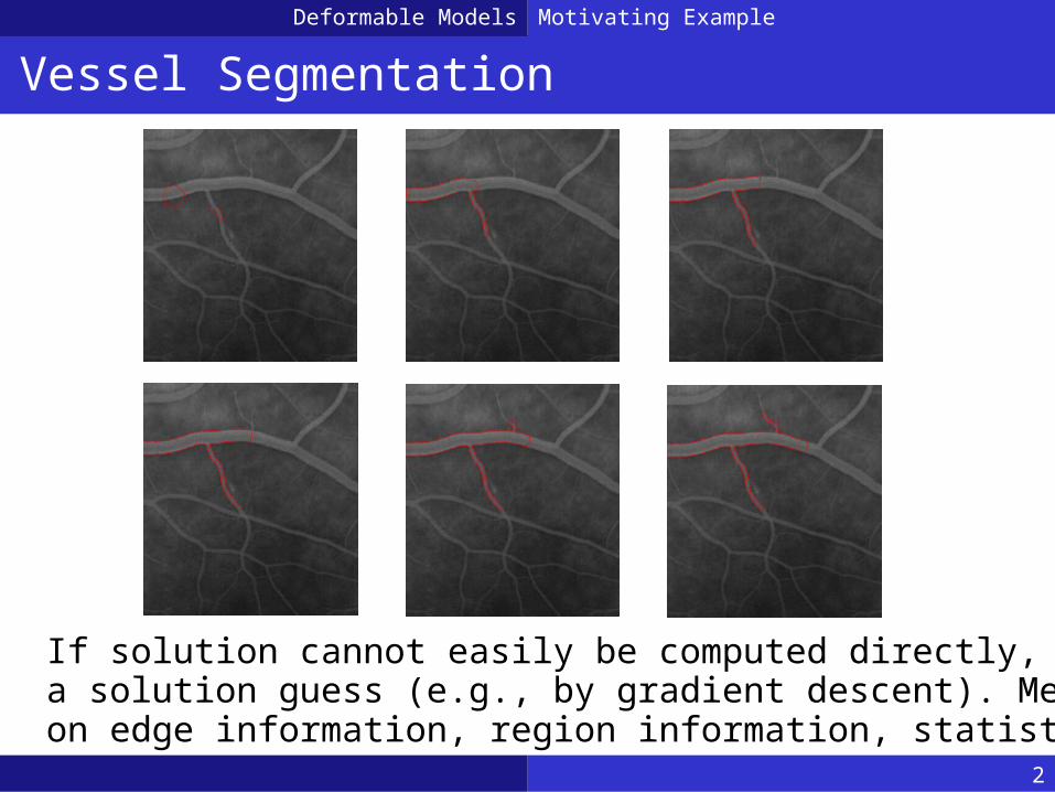
Vessel Segmentation
Motivating ExampleDeformable Models
If solution cannot easily be computed directly, iterative refinea solution guess (e.g., by gradient descent). Methods basedon edge information, region information, statistics, etc.

3
Heart Segmentation
Motivating ExampleDeformable Models
Image: Angenent et al.

4
Boundary Curve/Boundary Surface
Motivating ExampleDeformable Models

5
Pixel/Voxel vs. Boundary Representation
ParameterizationsDeformable Models
Classifying individual pixels versus finding an optimal separatingcurve/surface between object and background.

6
Parameterized Curve Evolution
ParameterizationsDeformable Models
Evolution should be geometric
Arclength is a specialparameterization, traversingthe curve with unit speed

7
Geometric Curve Evolution
ParameterizationsDeformable Models
moves “particles” along the curve
influences the curve’s shape
How is the speed determined?
The closed curve C evolves according to

8
Curve Evolution through Energy Minimization
Variational ApproachDeformable Models
Find curve that minimizes a given energy
Static curve evolution

9
Curve Evolution
Variational ApproachDeformable Models
Kass snake (parametric)
Geodesic active contour (geometric)
using the functionals
Minimize

10
Curve Evolution
ParameterizationsDeformable Models
leads to the Euler-Lagrange equations
Minimizing
Kass snake (parametric)
Geodesic active contour (geometric)

11
Curve Evolution
Variational ApproachDeformable Models
Kass snake (parametric)
Geodesic active contour (geometric)
results in the gradient descent flow
Minimizing
is an artificial time parameter

12
Active Contour
Variational ApproachDeformable Models
Minimizing
Active contour (geometric)
leads to
is an artificial time parameter to solve a static problem by gradient descent!

13
Particle-based approach
ImplementationDeformable Models
The curve is represented by a finite number of particles
Advantages• easy to implement• fast
Disadvantages• topological changes • particle spacing

14
Level Set Method
ParameterizationsDeformable Models
The curve is described implicitly as the zero level set of a higher dimensional function
The curve is described by
The level set function evolves as
Only works for closed curves or surfaces of codimension one.Osher, Sethian, "Fronts propagating with curvature dependent speed: Algorithms based on Hamilton-Jacobi formulations,"
Journal of Computational Physics, vol. 79, pp. 12-49, 1988.

15
Transporting Information
ParameterizationsDeformable Models
Flow information subject to the velocity field v.Velocity field can for example be the curve evolution velocity.

16
Level Set Method
ImplementationDeformable Models
Advantages
• topological changes• higher dimensions
Disadvantages
• computational complexity (narrow-banding)• velocity field extension• restriction to the evolution of closed curves or surfaces of codimension one
Image from http://math.berkeley.edu/~sethian/

17
Level Set Method
ImplementationDeformable Models
Zero level set of the level set function Φ corresponds to a curve in the plane.

18
Level Set Method: Some Evolution Examples
ImplementationDeformable Models
Curve evolutions with (left) and without (right) image information.
19
Mumford-Shah
Advanced ModelsDeformable Models
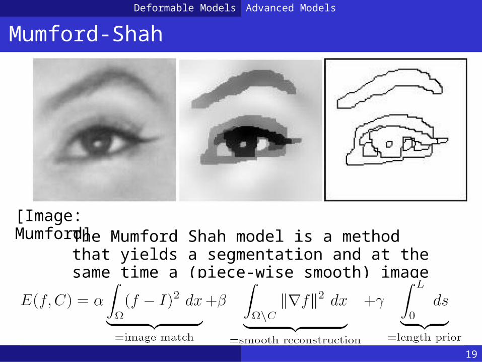
The Mumford Shah model is a method that yields a segmentation and at the same time a (piece-wise smooth) image reconstruction.
[Image: Mumford]

20
Chan-Vese (=Otsu thresholding w/ spatial regularity)
Advanced ModelsDeformable Models
Specialization of the Mumford-Shah model• two segments (foreground/background)• piecewise constant image models