communication behavior of a distributed operating...

Communication Behavior of a Distributed Operating System

Remzi H. Arpaci

Department of Electrical Engineering and Computer Science

Computer Science Division

University of California, Berkeley

Abstract

We present measurements of the communication behavior of a prototype distributed operating system, Solaris MC.

We employ three server workloads to drive our study: a build of the Solaris source tree, a synthetic web server, and a

parallel database. Our measurements reveal a number of facts, which have implications on design of Solaris MC, the

prototype implementation of Solaris MC, and the design of a message layer. We find that message traffic is centered

around nodes that house disks, a potential bottleneck. A file system that striped data across the cluster would avoid such

a problem. Most messages are medium sized, in the range of 68 to 256 bytes, indicating that message-layer support

for such messages is crucial. Further, messages are structured as a chain of two to three buffers, perhaps suggesting

the need for a gather interface to avoid additional buffer allocation and memory copies. Finally, request-response time

is quite high, due to overhead of the current message layer; this fact is perhaps most indicative of the prototype status

of the system. In any case, a low-overhead message layer would substantially improve overall performance.

Contents

1 Introduction 5

2 Background and Experimental Setup 8

2.1 Solaris MC �� 8

2.2 Experimental Method �� 10

2.2.1 Hardware �� 10

2.2.2 Tracing �� 10

2.2.3 Workloads �� 10

3 Workload Characterization 13

3.1 Overall Performance �� 13

3.2 CPU Utilization �� 14

3.3 System Calls and Context Switches �� 16

3.4 Summary �� 17

4 Message Traffic 18

4.1 Message Destinations �� 18

4.2 Message Sizes �� 22

4.3 Message Rates �� 26

4.4 Implications �� 30

5 Message Dependencies 32

5.1 Request-Response Workload �� 32


1

6 Anatomy of a Message 37

6.1 Buffer Chains �� 37

6.2 Protocol Overheads �� 38


7 Conclusions and Future Work 40

2

Acknowledgements

There are obviously many people to thank for making this report possible. First, I’d like to thank my advisor

Dave Patterson for his insight, guidance, and friendship. Without his insistence, I may never have completed

this report. I’d also like to thank my second reader, David Culler, whose advice “sort out the facets that are

arbitrary design decisions from those that are fundamental” I will remember for a long time to come.

Many thanks are extended to the members of the NOW group, from whom I’ve learned much in my first

three years at Berkeley. Though it is difficult to single out anyone in particular from this bunch, I would

like to especially thank Amin Vahdat, Rich Martin, and Alan Mainwaring for making Soda Hall a slightly

more tolerable place. I would also like to extend an extra note of thanks to Alan for owning an excellent

recording of Beethoven’s 7th.

Of course, none of this work would have been possible without the time and effort of the entire Solaris MC

group at Sun Labs. In particular, I would like to thank Yousef Khalidi for giving me such a great opportunity,

as well as his willingness to always lend an ear. I thank Moti Thadani for his excellent explanations of the

vagaries of STREAMs as well as many other enjoyable discussions. Without his assistance, none of this

would have been possible. I also thank Jose Bernebeu for his patience as well as all the help he gave me,

and Vlada Matena for his expert knowledge of various parts of Solaris. Finally, I thank Ken Shirriff for his

time and friendship. There was not a single member of the group who did not go out of their way to help

me at some time or the other.

I would like extend special thanks to my double co-worker, Keith Vetter, who helped gather some of the

measurements presented herein. Further, I thank Keith for introducing me to the magic of Bob Greenberg’s

music lectures.

I would like to thank my parents for all of the support, love, and encouragement they have given me

during the first years of my graduate studies. Their direction and advice has been invaluable, and without

them, I could not have achieved nearly so much.

Finally, I would like to thank my fiance, Andrea Dusseau, for everything she has given to me. There is

no other person I am indebted to on so many levels. Academically, her excellence has profoundly influenced

me. As a co-worker, I have learned uncountable lessons from her rigorous and careful pursuit of “the truth”.

She has been my sounding board, my expert reader, and my example to follow. For all of these, I thank her.

Personally, her love, support, and terrific friendship has kept me alive and happy for the past two years. I

3

am very lucky to have found such a wonderful person, and look forward to many years with her.

4

Chapter 1

Introduction

"The known is finite, the unknown infinite; intellectually

we stand on an islet in the midst of an illimitable ocean

of inexplicability. Our business in every generation is

to reclaim a little more land."

-Thomas H. Huxley

Distributed systems have long been an active area of research [8, 12, 22, 24, 25]. A distributed system

is comprised of many components, including process management, networking, and file systems. Although

the requirements of these various services are eclectic, they have a common need: to communicate.

Along these lines, early work often indicated that achieving high network performance was paramount

to attaining good overall distributed system performance [11, 31]. Not surprisingly, many researchers have

focused their efforts on design and implementation of fast communication protocols [4, 7, 9, 14].

The recent arrival of high-speed, switch-based local-area networks has improved communication per-

formance by an order of magnitude [2, 6]. The bandwidth of many of these networks is in the 100 MB/s

range, and, by making use of lightweight communication protocols, one-way end-to-end times are in the

range of 10 to 100 microseconds [18, 32]. This provides a quantum leap over the shared-medium 10 Mb/s

Ethernet upon which many previous systems were designed.

With this radical change underway, it is important to understand and characterize how modern distributed

systems make use of new communication technologies. What are the necessary performance characteristics

of the underlying network? What functionality must a message layer provide? What do these measurements

5

Fact Implication

1. Most message traffic is centered around disks Striping file system would be valuable

2. Medium-sized messages account for most traffic Message-layer must support medium-sized messages

3. Request-response time is high Need low-overhead message layer

4. Most messages are a chain of two/more buffers Message-layer support for gathering interface?

Table 1.1: In the first column, we present our main findings from measurements of communication behaviorof Solaris MC. The second column shows potential implications on the design and implementation of thesystem and its message layer.

tell us about the structure of the distributed system itself?

To begin to answer these questions, we have instrumented the communication layer of a distributed

operating system. The system under scrutiny is Solaris MC, a prototype cluster operating system [15]. MC

is novel in a number of ways: it extends a real, commercial kernel (Solaris) into a distributed system; further,

it does so by building on top of a distributed object system based on CORBA [30]. MC extends the file

system, process management, networking, and I/O subsystems of Unix to provide users with a single-system

image.

Although MC provides an interesting measurement testbed, it is currently in the early stages of de-

velopment. Many aspects of the system have not yet been optimized. This directly affects some of our

measurements, especially those that are timing-sensitive. For example, the load placed on the message

subsytem is not very high. Other measurements, including the sizes and destinations of messages, are not

affected. Bearing this in mind, we attempt to separate out results that come from poor implementation or

design decisions from those that are fundamental.

To drive the traces of communication behavior, we employ three server workloads: a build of the Solaris

source tree, a web server responding to a synthetic stream of HTTP requests, and a database performing

a series of debit/credits. Our analysis consists of four progressive steps. First, we trace resource usage

statistics to characterize the workloads. Then we trace aggregate communication between the nodes of the

cluster. From this data, we derive message distributions and rates. Next, since nearly all communication in

Solaris MC is based on requests and subsequent responses, we instrument a higher level of the system to

unveil communication dependencies. We conclude by examining the structure of each individual message

6

to understand the type of interface a message layer should provide.

Our measurements reveal a number of facts, highlighted in Table 1.1. We now discuss our results and

their implications on the design of Solaris MC, its prototype implementation, and the design of a message

layer.

We find that message traffic in the cluster is centered around the disks. The use of a striped file system

could avoid potential disk bottlenecks. Other global services, such as the network port name-space manager,

may need to be distributed as well or suffer from similar bottlenecks.

We also find that most messages, roughly 80% across all workloads, are in the range of 68 to 256 bytes.

Support for these message sizes is critical in the design of a message layer. Not surprisingly, most of the

data is usually sent in larger messages, frequently 4 KB or more. Avoiding memory copies and other actions

that are a function of message size would be beneficial.

By instrumenting the object subsystem, we find that the prototype implementation of Solaris MC suffers

from unusually high request-response times, about 1.65 �� for a simple request-response. About 60% of

this can be attributed to the high-overhead of the STREAMS-based transport. The implication in this case

is obvious: the system is in desperate need of a low-overhead transport layer. The current cost of the object

infrastructure is also quite high, accounting for roughly 30% of the 1.65 �� . Thus, in an ideal case where

the transport layer is fast, the overhead of the object system becomes quite significant.

Finally, we find that most messages are formed of a chain of two to three buffers. A gathering interface

could be of some benefit, saving the cost of a memory-to-memory copy and buffer allocation for most

messages. These chains are a by-product of the design of the object subsystem, which attaches a header as

a separate buffer to each message. Some implementation effort could potentially remedy the situation.

What follows is an outline of the rest of the paper. The next section gives a brief overview of the Solaris

MC operating system and describes the hardware configuration and methodology used in the study. In

Section 3, we describe the workloads used to drive most of the study. In Section 4, we begin with the first of

the measurements, which are aggregate summaries of communication patterns. In Section 5, we understand

this at a higher level, viewing all communication as request-response pairs. Finally, in Section 6, we detail

the structure of a message and the implications on the layers below. We conclude and give future directions

in Section 7.

7

Chapter 2

Background and Experimental Setup

In this section, we describe the Solaris MC system. First, we give a high-level overview of the concepts and

philosophy behind the system. Then, we outline the particulars of the experimental environment.

2.1 Solaris MC

Solaris MC [15] is a prototype multi-computer operating system, where a multi-computer is a cluster of

homogeneous computers connected via a high-speed interconnect. Solaris MC provides a single-system

image, constructing the illusion of a single machine to users, applications, and the external network. The

existing Solaris API/ABI is preserved, such that existing Solaris 2.x applications and device drivers run

without modification. Finally, MC provides support for high availability [19].

Solaris MC is comprised of four major subsystems: the file system, process management, networking,

and I/O. Extensions were made to each of these components of a normal Solaris kernel in order to attain

the aforementioned goals. We now briefly explain each component of MC, as well as the underlying object

substrate.

The Solaris MC file system, PXFS (the proxy file system), extends the local Unix file system to a

distributed environment [26]. In PXFS, all file access is location transparent. A process anywhere in the

system can open a file located upon any disk in the system. PXFS accomplishes this by interposing at the

vnode layer [34], where PXFS can intercept file operations and forward them to the correct physical node.

Further, all nodes see a single path hierarchy for all accessible files. To ensure UNIX file system semantics,

coherency protocols are employed. For performance, PXFS makes use of extensive caching based on

8

techniques found in Spring[16], and will eventually provide zero-copy bulk I/O of large data objects.

The second major subsystem is process management. In Solaris MC, process management is globalized

such that the location of a process is transparent to the user. While threads of a process are restricted to

the same physical node, the process may be anywhere in the system. Currently, the system makes use of

remote execution facilities to run jobs on other nodes in the system. Process management is implemented as

a virtual layer (vproc) on top of existing Solaris process management code. By tracking the state of parent

and children processes, process groups, and sessions, MC supports POSIX process semantics. To access

information about processes, Solaris MC extends the /proc file system (e.g. for use by ps, debuggers, and

so on) to a global /proc which covers all processes within the system. Solaris MC will also soon provide

migration facilities and remote fork capability.

Global networking is the third subsystem of Solaris MC. For network applications, MC creates a single

system image with respect to all network devices in the system. Thus, a process on any node in the system

has the same network connectivity as any other process, regardless of location. Three key components are

involved in achieving this end: global management of the network name space, distributed multiplexing,

and distributed de-multiplexing.

A distributed program, known as the SAP-server, manages the global network name space. The SAP-

server prevents simultaneous allocation of TCP/IP ports to different processes spread across the nodes of

the cluster. Outgoing packets are processed on the same node as the application, and then forwarded if

necessary to the appropriate network interface. Similarly, a packet filter intercepts incoming packets and

directs them to the correct node.

The final subsystem of Solaris MC, the global I/O subsystem, extends Solaris to allow for cross-node

device access. To accomodate this cross-node functionality, changes were made to the following: device

configuration, loading and unloading of kernel modules, device naming, and providing process context for

drivers.

All of these subsystems are built on top of a C++ runtime environment for distributed objects, known

as the Object Request Broker (ORB). The ORB can be viewed as the object communication backplane that

performs all the necessary work to support remote object invocations. In Solaris MC, the ORB also provides

other features such as reference counting on objects as well as support for one-way communication. For a

full description of the ORB, see [5].

9

2.2 Experimental Method

This section describes our experimental method. First, we describe the hardware and software platform

used for the experiments. Then we explain how we instrumented Solaris MC, and the performance effects

that arose from the instrumentation. Finally, we give details on the workloads used to drive the simulations.

2.2.1 Hardware

The cluster of MC machines consists of SPARC-5s, SPARC-10s, and SPARC-20s, each running a copy

of a modified version of Solaris 2.5, which includes the changes necessary to support Solaris MC. Most

experiments are performed on an 8-CPU, 4-node cluster of SPARC-10s, each with 64 MB of memory. Each

machine has an Ethernet connection to the outside world, a connection to the fast intra-cluster network, the

Myrinet local-area network [6], and possibly an extra disk which acts as part of the global file system. In

Section 5, the cluster configuration is slightly different; it is explained further therein.

2.2.2 Tracing

To trace the communication behavior of Solaris MC, we make extensive use of the TNF tracing facility in

Solaris 2.5 [29]. This utility allows events in the kernel to be time-stamped and logged to a kernel buffer,

which can then easily be extracted and analyzed. Each call to log an event takes roughly 7 microseconds;

therefore, insertion of many such calls along a critical path can seriously alter results. Thus, when performing

timing measurements, we judiciously inserted logging statements, only measuring events that were long

enough such that the timing overhead was insignificant. Even in these cases, we took care to subtract out

the timing overhead.

2.2.3 Workloads

Throughout most of the paper, we utilize three workloads to drive the system. As illustrated in Figure 2.1,

these workloads use slightly different hardware configurations. The first workload, make, performs a large,

parallel make of the Solaris MC source tree. A shell on��

1 starts the make, which uses the rexec system

call to distribute jobs to the various nodes of the system. The disk holding the source tree is attached to��

3. This workload stresses remote execution facilities as well as PXFS.

10

The second workload, web, is based on the Spec WWW benchmark [28]. In this benchmark, an external

stream of HTTP requests is generated and sent to the MC cluster, each node of which is running a copy

of the NCSA httpd server [23]. All requests are sent to��

2 which is connected to an Ethernet network

interface. After a request is received, the networking subsystem redirects the traffic for this connection to

one of the nodes in the system, similar to the Mach packet filter [21]. All responses are forwarded from the

responding cluster node to��

2 and then back to the original source. The disk containing the HTTP files

is connected to� �

2. This workload heavily utilizes the MC networking sub-system, and potentially the

caching features of the file system.

Lastly, the database workload performs a series of transactions on the Oracle Parallel Database��

.

Simple debit/credit transactions are performed in parallel on all nodes, while the disk containing the database

on it is attached to��

4. This workload stresses aspects of the global file system.

11

MC 3 4MC

1MC

P

P

P

P

MC

P

Make

P

P

P2

rexec()rexec()

rexec()

MC 3 4MC

1MC N I

P

P

P

P

P

MC

Web

P

P

P

2

TCP trafficTCP traffic

TCP traffic

External HTTP Requests

MC 3 4MC

1MCP

P

P

P

MC

P

Database

P

P

P

2

Transactions Transactions

Transactions

Figure 2.1: Workload Setup. The upper-left diagram shows the experimental setup for the make workload.Note that each workstation has two processors, as indicated by the circled P symbol. A parallel make isstarted on

��1, which remotely executes jobs on all four workstations. The disk containing the Solaris

source tree is attached to� �

3. The upper-right diagram depicts the web workload setup, with externalHTTP requests streaming into

� �2. Traffic is distributed among the machines in a round-robin fashion,

and responses proceed through� �

2 back to the source. The disk containing the requested file is alsoattached to

� �2. The lower diagram shows the database workload setup, with the disk attached to

� �4.

For this experiment, all machines perform transactions for a fixed time period.

12

Chapter 3

Workload Characterization

In the process of gathering workloads for a study of a distributed system, it is important to concentrate on

finding programs that will stress system services. In this section, we characterize the three workloads that

drive the study and show that they do indeed make use of operating system services. First, we present the

overall performance of each of the workloads. Then, to give some insight on the nature of the workloads,

we give breakdowns of CPU usage and two other measures of the system, system calls and context switches

per second.

3.1 Overall Performance

This section shows how the workloads perform without any tracing activated. Table 3.1 gives either the run

time and the rate of operation for each of the workloads. The run-time for the last two workloads is chosen

by the experimenter, whereas the run-time for the make workloads is determined by a fixed amount of work.

The rate of make reveals the number of compilations per second. In the case of the web workload, external

clients perform HTTP get operations to fetch a specified file, and the rate measures the number of HTTP

operations per second. For the database workload, clients within the system perform simple debit/credit

operations. Due to legal issues, the rate of the last workload is not revealed. Since this is a prototype system,

one can see that the performance of the system is not particularly spectacular (nor has it yet been tuned for

performance); in Section 5, we will see the main reason for this. Each of the last two workloads run for a

fixed four minute period.

13

Workload Time Rate

make 9 mins, 53 secs 0.35 compiles/secweb 4 mins, 01 secs 8 HTTP ops/sec

database 4 mins, 03 secs N.A.

Table 3.1: Benchmark Performance. The total performance in time and as a rate of each benchmark.

3.2 CPU Utilization

Figure 3.1 shows the CPU utilization of each workload over the lifetime of an experiment. To collect this

data, a user-level daemon awakens every second and collects statistics. CPU usage consists of four distinct

parts: “user”, the percent of time spent in the running program, “system”, the percent of time spent in the

operating system, “wait”, the percent of time spent waiting for a disk I/O to return, and “idle”, the remaining

difference. Note that the graphs are cumulative; thus, the “system” line is actually the sum of “system” and

“user” time, and so forth.

0%

100%

200%

300%

400%

500%

600%

700%

800%

0 100 200 300 400 500 600 700

CP

U P

erce

ntag

e

Time (Seconds)

CPU Profile for Make

WaitSystem

User

0%

100%

200%

300%

400%

500%

600%

700%

800%

0 50 100 150 200 250 300

CP

U P

erce

ntag

e

Time (Seconds)

CPU Profile for WWW

WaitSystem

User

0%

100%

200%

300%

400%

500%

600%

700%

800%

0 50 100 150 200 250 300

CP

U P

erce

ntag

e

Time (Seconds)

CPU Profile for Database

WaitSystem

User

Figure 3.1: Cumulative CPU Utilization. The cumulative CPU utilization, split into user, system, andwait time is displayed over time for each workload (the rest is idle) . The maximum CPU percentage at agiven moment is 800%, since each of 8 CPUs can have at a peak 100% utilization. Note that the graphs arecumulative; system time is the sum of system and user time, and wait time is the sum of all three. The whitespace from 800% down to the top-most line, wait time, is idle time.

For the make workload, we see the utilization changes over time. At first, the makefile runs through a

sequential portion, and thus the utilization for the first 60 seconds is low, at roughly 1.2 processors worth of

CPU. Then the parallel portion begins, and we see a relatively constant utilization of about 4 to 5 processors,

with some spikes up to the peak 6. Finally, the make ends with a long link phase at roughly 600 seconds.

On average, this workload spends 17% of the time in user mode and 12% of the time in system mode, for a

total CPU usage of 30%.

14

1,1

1,2

2,1

2,2

3,1

3,2

4,1

4,2

0 100 200 300 400 500 600 700

Mac

hine

, CP

U N

umbe

r

Time (Seconds)

Individual CPU Traces (Make)

1,1

1,2

2,1

2,2

3,1

3,2

4,1

4,2

0 50 100 150 200 250 300

Mac

hine

, CP

U N

umbe

r

Time (Seconds)

Individual CPU Traces (WWW)

1,1

1,2

2,1

2,2

3,1

3,2

4,1

4,2

0 50 100 150 200 250 300

Mac

hine

, CP

U N

umbe

r

Time (Seconds)

Individual CPU Traces (Database)

Figure 3.2: Individual CPU Utilization. The CPU utilization (the sum of user and system time) over timeis displayed per CPU for the cluster. The Y axis shows

� �1 through

� �4, as well as each CPU (1 or 2)

on those machines. For example, 2,1 implies� �

2, CPU 1.

The web workload displays significantly different behavior. The workload starts at around the 30-second

mark and ends 4 minutes later. As you can see, more than three quarters of the CPU is utilized at all times

throughout the run. One particular item of interest is the two dips in the graph, at about 50 and 250 seconds.

At those times, the transport layer lost a message. Thus, what you see is a hiccup when a message times out

and is retransmitted. After this mishap, the system continues normally. The web workload is most sensitive

to this type of failure. If� �

2 stops forwarding HTTP requests to other nodes in the system, the other nodes

will have no work to do in that time and will remain idle. The main point of interest is the large percentage

of time spent in the system, roughly 21% of total time, or 31% of non-idle time.

Finally, the figure reveals that the database workload makes very little use of the CPU. Of the small

fraction that is utilized, most is spent in system time (14% of total time, and 80% of non-idle time). User

time accounts for only 3% of total time, and the workload spends 12% of the time waiting for disk requests.

To show how the load is balanced across the cluster, Figure 3.2 presents CPU utilization per processor.

For this set of graphs, we view the sum of user and system time.

For the make workload, we can see that the load is fairly well balanced throughout, although nodes 2

and 4 finish somewhat sooner than the other two. Note that� �

3 is the busiest node, since it houses the

disk where the source tree is located. The diagram of the web workload shows how all processors are well

utilized throughout the benchmark. Again, note the two dips in the CPU graphs when a packet was lost.

Lastly, when considering the database workload, again note the relatively low and constant CPU usage

across all machines. In this case,� �

4 is the busiest node, again due to the presence of the disk.

15

0

1000

2000

3000

4000

5000

6000

0 100 200 300 400 500 600

Sys

tem

Cal

ls /

Sec

ond

Time (Seconds)

System Call Profile (Make)

0

1000

2000

3000

4000

5000

6000

0 50 100 150 200 250

Sys

tem

Cal

ls /

Sec

ond

Time (Seconds)

System Call Profile (Web)

0

1000

2000

3000

4000

5000

6000

0 50 100 150 200 250

Sys

tem

Cal

ls /

Sec

ond

Time (Seconds)

System Call Profile (Database)

Figure 3.3: System Calls per Second. An aggregate of system calls/second across all workstations.

0

1000

2000

3000

4000

5000

6000

0 100 200 300 400 500 600

Con

text

Sw

itche

s / S

econ

d

Time (Seconds)

Context Switch Profile (Make)

0

1000

2000

3000

4000

5000

6000

0 50 100 150 200 250

Con

text

Sw

itche

s / S

econ

d

Time (Seconds)

Context Switch Profile (WWW)

0

1000

2000

3000

4000

5000

6000

0 50 100 150 200 250

Con

text

Sw

itche

s / S

econ

d

Time (Seconds)

Context Switch Profile (Database)

Figure 3.4: Context Switches per Second. An aggregate of context switches/second across all workstations.

3.3 System Calls and Context Switches

The CPU utilizations have indicated that the workloads are making use of the operating system. To show that

the operating system is under some duress, we now show the number of system calls and context switches

per second.

In Figure 3.3, we see the aggregate number of system calls per second performed by each of the

workloads. From this, we can see that all of the workloads make fairly heavy use of operating system services.

Of the three workloads, make performs the fewest, with an average of 2297 per second. Presumably most of

the calls are file system related. The web workload is the most intense, performing an aggregate average of of

4633 syscalls per second. This workload makes use of the file system as well as the networking subsystem,

and thus is frequently crossing the user-space/kernel boundary. Finally, database shows constant system

call rates at around 3096 per second across the cluster, presumably stressing the file system.

On a SPARC-10 running Solaris 2.5, trapping into and returning from the kernel takes roughly 6 � � . If

a workload performs system calls at a rate of 5000 per second, about 30 �� out of every second is spent

crossing the user-kernel boundary. This about 3% of of the time is spent in kernel call overhead, a small but

16

noticeable fraction.

We next examine the total number of context switches per second across all workstations in the cluster.

This counts the number of times the low-level context switch routine is called inside the kernel. Since a

process that goes to sleep during a system call may force a context switch, this figure and the last may be

somewhat correlated.

Figure 3.4 contains the data. From this figure we see more evidence that the operating system is under

some strain during the execution of the workloads, as well as the same general trends we saw in the previous

figure. The make, web, and database workloads average 1334, 2850, and 2851 context switches per second.

One interesting point about the context switch rate is its intensity; if a context switch takes about 30 � � [20],

3000 switches per second implies 3000 � 30 � �� 90 � 000 � �� 90 �� of time spent switching per second.

90 milliseconds of switch time every second is almost 10% of all time.

3.4 Summary

In this section, we have used a number of measures of system usage – CPU utilization, system call rates,

and context switch rates – to indicate that the workloads are operating-system intensive. We have seen that

40%, 30%, and 80% of all non-idle time is spent in the operating system, for the make, web, and database

workloads, respectively. All the workloads perform a heavy number of system calls, spending 1% to 2%

of the time trapping into the kernel, and the system switches contexts frequently during all workloads; in

section 5, we will gain some insight as to the frequency of these switches. A better characterization of the

workloads is in order, but with the purposes of this study in mind, we leave that to future work.

17

Chapter 4

Message Traffic

In the last section, we introduced the three workloads that drive our study. In this section, we trace the

messages sent between the nodes of the cluster during each of the workloads. First, we trace the destinations

of messages in the cluster, as well as how many bytes were sent from node to node. We next give cumulative

breakdowns of message sizes. Finally, the rate at which each node sends messages is presented. All

measurements are of kernel-kernel traffic, that is, messages sent through the intra-cluster interconnect.

Although there is some kernel-user traffic – for example, the name server is implemented in user space –

the amount of such traffic is negligible. Also, note that all nodes are “workers”, performing some fraction

of the work necessary to complete the workload at hand; in addition to this, some nodes serve a special

purpose during the workload, which we will indicate where necessary.

4.1 Message Destinations

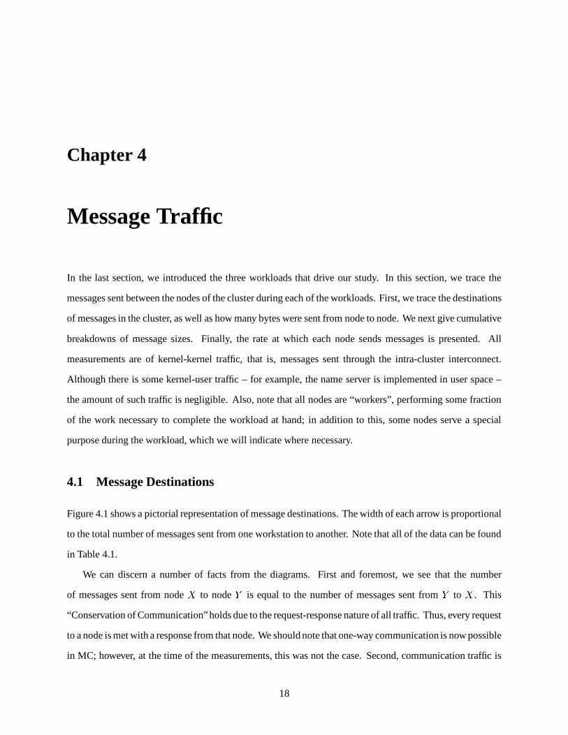
Figure 4.1 shows a pictorial representation of message destinations. The width of each arrow is proportional

to the total number of messages sent from one workstation to another. Note that all of the data can be found

in Table 4.1.

We can discern a number of facts from the diagrams. First and foremost, we see that the number

of messages sent from node�

to node � is equal to the number of messages sent from � to�

. This

“Conservation of Communication” holds due to the request-response nature of all traffic. Thus, every request

to a node is met with a response from that node. We should note that one-way communication is now possible

in MC; however, at the time of the measurements, this was not the case. Second, communication traffic is

18

MC 3 4MC

1MC

15,650

7,215

MC

Make

2

MC 3 4MC

1MC 11,739

6,398

N IMC

Web

2

MC 3 4MC

1MC

9,159

8,221

8,190

MC

Database

2

Figure 4.1: Message Destinations. The width of each bar is proportional to the number of messages sentfrom one node to another node. In the make diagram, the maximal arrow is between nodes 1 and 3, with15,650 messages exchanged each way. For web, nodes 2 and 1 exchange 11,739 messages, and finally fordatabase, nodes 2 and 4 each send 9,159 messages to each other. All figures are scaled to the same basenumber, and thus are readily comparable.

19

often centered where disks are attached; this will be discussed further below.

For the make workload, we see a skewed traffic pattern across the nodes. Though all nodes do

communicate with all other nodes, most messages were sent to/from� �

3, since the disk containing the

source tree is attached to that node.

Message traffic is also non-uniform in the web workload. As the figure indicates, two nodes are of

special interest,� �

1 and��

2. The presence of the “external” network interface on node 2 reveals why

traffic is heavy there, as it serves as the cluster’s gateway to and from the Internet. 1 Each HTTP request

is routed through��

2, with a round-robin selection among all nodes determining which node handles the

request. After fetching the requested file, a node routes the message back to� �

2 and then back to the

requester.

The other hot-spot in the web workload is� �

1, where the Service Access Point Server (SAP-server)

manages the global port name space. Thus, when a connection is opened or closed, communication with the

SAP-server on node 1 must occur. While in this MC configuration the SAP-server runs on a single node, in

practice it could be a distributed program, perhaps with each node managing a portion of the name space.

Co-locating the SAP-server and nodes with external connections would lessen message traffic, by reducing

it to local inter-process communication.

Finally, for the database workload, we see that all traffic is centered around the disk where the database

resides. A more realistic environment would spread disks across all the nodes, and could lead to more

evenly balanced traffic patterns. However, this balance would only be achieved if the access patterns were

naturally balanced, since Solaris MC takes no explicit action to balance file system load across the cluster.

Although the previous figures show how message communication is spread across the cluster, it does not

show how many bytes are sent to and from each node. Figure 4.2 weights the previous graph by total bytes

sent. Thus, the width of each arrow is proportional to the total number of bytes sent to that workstation.

This total includes user payload as well as ORB headers, which are fundamental to the operation of the

system, but not transport headers, which are implementation specific.

For the make workload, most traffic comes out of� �

3. The reason for this is that node 3 plays the

role of file server for this experiment, and all nodes request file blocks from it. Further, modified file blocks

must eventually return to node 3. In this workload, we find that incoming traffic to node 3 totals 13 MB,

1Though all workstations have Ethernet connections, for the experiment, all traffic is routed through �� 2 . An alternative MCconfiguration allows TCP messages to return through the network interface of each of the other nodes.

20

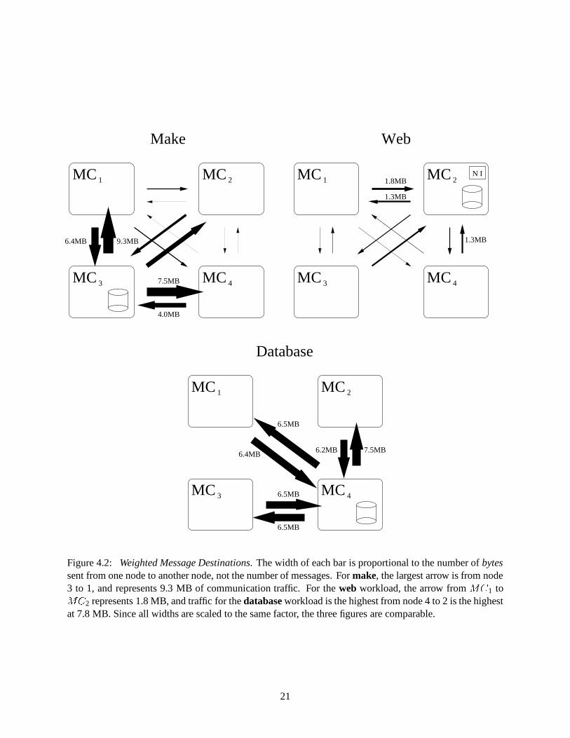
MC 3 4MC

1MC

9.3MB6.4MB

4.0MB

7.5MB

MC

Make

2

MC 3 4MC

1MC 1.8MB

1.3MB

1.3MB

N IMC

Web

2

MC 3 4MC

1MC

7.5MB6.2MB

6.5MB

6.4MB

6.5MB

6.5MB

MC

Database

2

Figure 4.2: Weighted Message Destinations. The width of each bar is proportional to the number of bytessent from one node to another node, not the number of messages. For make, the largest arrow is from node3 to 1, and represents 9.3 MB of communication traffic. For the web workload, the arrow from

��1 to

��2 represents 1.8 MB, and traffic for the database workload is the highest from node 4 to 2 is the highest

at 7.8 MB. Since all widths are scaled to the same factor, the three figures are comparable.

21

and out-bound communication is 21 MB, perhaps indicating more bytes were read than written.

For the web workload, the byte-weighted diagram reveals that most data flows to��

2 from each of the

other nodes (about 1.4 MB from nodes 3 and 4, and 1.8 MB from node 1). The only other heavy byte flow

is to� �

1 from� �

2; as mentioned before, this is SAP-server traffic. Note that the total bytes sent in this

workload is significantly less than the other two.

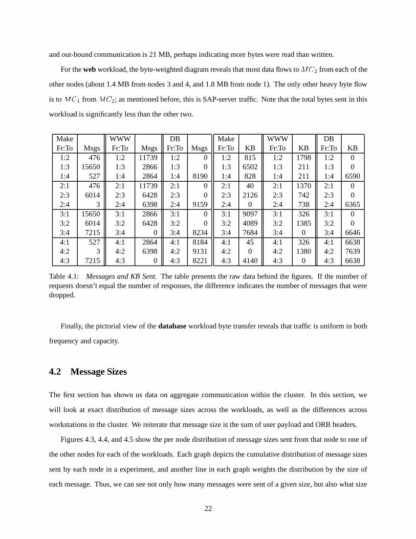
Make WWW DBFr:To Msgs Fr:To Msgs Fr:To Msgs1:2 476 1:2 11739 1:2 01:3 15650 1:3 2866 1:3 01:4 527 1:4 2864 1:4 81902:1 476 2:1 11739 2:1 02:3 6014 2:3 6428 2:3 02:4 3 2:4 6398 2:4 91593:1 15650 3:1 2866 3:1 03:2 6014 3:2 6428 3:2 03:4 7215 3:4 0 3:4 82344:1 527 4:1 2864 4:1 81844:2 3 4:2 6398 4:2 91314:3 7215 4:3 0 4:3 8221

Make WWW DBFr:To KB Fr:To KB Fr:To KB1:2 815 1:2 1798 1:2 01:3 6502 1:3 211 1:3 01:4 828 1:4 211 1:4 65902:1 40 2:1 1370 2:1 02:3 2126 2:3 742 2:3 02:4 0 2:4 738 2:4 63653:1 9097 3:1 326 3:1 03:2 4089 3:2 1385 3:2 03:4 7684 3:4 0 3:4 66464:1 45 4:1 326 4:1 66384:2 0 4:2 1380 4:2 76394:3 4140 4:3 0 4:3 6638

Table 4.1: Messages and KB Sent. The table presents the raw data behind the figures. If the number ofrequests doesn’t equal the number of responses, the difference indicates the number of messages that weredropped.

Finally, the pictorial view of the database workload byte transfer reveals that traffic is uniform in both

frequency and capacity.

4.2 Message Sizes

The first section has shown us data on aggregate communication within the cluster. In this section, we

will look at exact distribution of message sizes across the workloads, as well as the differences across

workstations in the cluster. We reiterate that message size is the sum of user payload and ORB headers.

Figures 4.3, 4.4, and 4.5 show the per node distribution of message sizes sent from that node to one of

the other nodes for each of the workloads. Each graph depicts the cumulative distribution of message sizes

sent by each node in a experiment, and another line in each graph weights the distribution by the size of

each message. Thus, we can see not only how many messages were sent of a given size, but also what size

22

0%

20%

40%

60%

80%

100%

64 128 256 512 1 K 2 K 4 K 8 K

Per

cent

Message Size (Bytes)

Message Size Breakdown (MC_1) (Make)

Cumulative by Message CountCumulative by Message Size

0%

20%

40%

60%

80%

100%

64 128 256 512 1 K 2 K 4 K 8 K

Per

cent




0%

20%

40%

60%

80%

100%

64 128 256 512 1 K 2 K 4 K 8 K

Per

cent




0%

20%

40%

60%

80%

100%

64 128 256 512 1 K 2 K 4 K 8 K

Per

cent




Figure 4.3: Message Size Distribution for the make workload. The lines count the number of messagessent from each node. No message is smaller than 68 bytes, and about 80% of all messages are smaller than256 bytes. However, most data is transferred in big chunks; 70% of data is shipped in units of 4 KB ormore.

packets transferred most of the data.

Figure 4.3 shows this breakdown for the make workload. By observing the cumulative distribution of

message sizes in each of the diagrams (the upper-most line), we see that most messages are small. In fact,

across all workstations, 80% of messages are less than 256 bytes. Request-response traffic encourages this

to some extent; usually, only one direction of a request-response will transfer a large chunk of data. Note

that no message is smaller than 68 bytes; specific support for messages of less than that size in this domain

is not useful.

The lower line in the graphs weights the distribution by message size. Thus, while most messages

are small, most data is in fact transferred in large messages. This seems to be one of the few “Truths in

Computer Science”; even though most data is transferred in large objects, most objects are small. For nodes

23

0%

20%

40%

60%

80%

100%

64 128 256 512 1 K 2 K 4 K 8 K

Per

cent


Message Size Breakdown (MC_1) (WWW)


0%

20%

40%

60%

80%

100%

64 128 256 512 1 K 2 K 4 K 8 K

Per

cent




0%

20%

40%

60%

80%

100%

64 128 256 512 1 K 2 K 4 K 8 K

Per

cent




0%

20%

40%

60%

80%

100%

64 128 256 512 1 K 2 K 4 K 8 K

Per

cent




Figure 4.4: Message Size Distribution for the web workload. The lines count the number of messages sentfrom each node. No message is smaller than 68 bytes, and about 80% of all messages are smaller than 176bytes. Across all machines, only 30% of all messages could be considered large, in this case larger than 1KB. This can be attributed to the synthetic nature of the workload.

1, 3, and 4, roughly 80% of data is transferred in blocks of 4 KB or larger, and for node 2 that number is

about 70%. Of course, message sizes in this case are directly influenced by file sizes; previous studies of

file sizes in Unix environments have shown that these have a similar “most files small, most data in large

files” distribution[3].

In Figure 4.4, we see that the message sizes for the web workload are much more regular than the make

workload; there are only about 10 different message sizes sent throughout the lifetime of the experiment.

Two nodes,��

3 and� �

4, have almost identical distributions, as might be predicted from 4.1. In those

graphs, roughly 90% of messages are less than 256 bytes. The difference here is that only 40% of all bytes

are transferred in what could be considered “large” messages, in this case, 1.5 KB. Note that this is highly

dependent on the HTTP request; for this experiment, all requests are for a 1500-byte file. A more diverse

24

0%

20%

40%

60%

80%

100%

64 128 256 512 1 K 2 K 4 K 8 K

Per

cent


Message Size Breakdown (MC_1) (Database)


0%

20%

40%

60%

80%

100%

64 128 256 512 1 K 2 K 4 K 8 K

Per

cent




0%

20%

40%

60%

80%

100%

64 128 256 512 1 K 2 K 4 K 8 K

Per

cent




0%

20%

40%

60%

80%

100%

64 128 256 512 1 K 2 K 4 K 8 K

Per

cent




Figure 4.5: Message Size Distribution for the database workload. The lines count the number of messagessent from each node. No message is smaller than 68 bytes, and about 80% of all messages are smaller than152 bytes. Again, most data is transferred in big chunks; 90% of data is shipped in units of 4 KB or more.

non-synthetic workload would directly correlate with a more diverse message pattern. Again note that no

message is smaller than 68 bytes.

The traffic coming out of� �

2 is comprised of only small messages; this node relays requests to other

nodes, not replies, which carry the larger payload. The traffic to��

1 is slightly different than the rest.

We again attribute this to the SAP-server, whose presence leads to small message exchanges necessary to

manage the global port name space.

The database workload in Figure 4.5 gives us one additional data point on the spectrum of message

distributions. It bears similarity to the make workload in that roughly 80% of messages are small (152 bytes

or less), and that there are few large messages that move most of the data (90% of data is transferred in 4 KB

blocks). On the other hand, there are only a few distinct message sizes, similar to the web workload; in this

25

case, roughly 8 message sizes. As we said, a more realistic database workload would run on more disks.

However, this would not significantly alter the message size distributions (each node would perform more

of the same request-responses); it would simply serve to balance the traffic across the nodes more equally.

4.3 Message Rates

By examining the message size distributions, we have observed a “size” burstiness in the traffic: many

small protocol messages for every large data packet. In this section, we try to establish whether a “time”

burstiness exists.

Figures 4.6, 4.7 and 4.8 depict the number of messages sent from each node each second over the

life of each experiment. As in the last set of graphs, for each workload, there are four diagrams, one per

workstation.

During the make workload, each node communicates in a relatively bursty manner. Workstations have

periods where hundreds of messages are sent in a given second, and a quarter of that the next second.

However, we can see that� �

2 and��

4 send the fewest messages over time, with an average rate of

15 and 18 messages per second, respectively. As noted before, these two nodes are just “workers”; while

all nodes partake in the make, these have no other special responsibilities.��

1 differs because the make

master is executing there. Thus, additional messages are necessary for rexec system calls that distribute

the work among the nodes.��

1 averages 31 message per second over the experiment. Finally,��

3, the

file server, is under the most strain, as it needs to respond to many requests to get files. We can readily see

this in the graph;��

3 averages 50 messages per second, notably more than the other nodes.

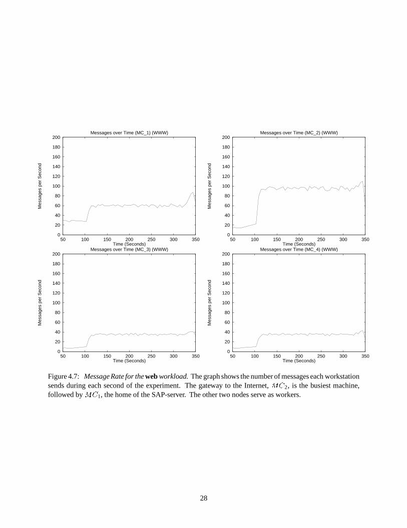
Once again, the web workload shows how workload-sensitive the traffic patterns are. In Figure 4.7,

observe that all nodes are constantly sending messages from time 100 seconds onward, when the experiment

began. The only qualitative difference is in quantity.� �

2 sends the most messages (75 per second), since

it routes all traffic,��

2 with the SAP-server sends somewhat less (53 per second), and the two “worker”

nodes,��

3 and��

4, even less, averaging about 28 messages per second each.

The database workload proves to be more similar to the web workload, with all nodes communicating

at near constant rates. This can be attributed to the nature of the workload, in which each node continually

performs transactions. While nodes 1, 2, and 3 all send about 30 messages per second, the file server, node

4, sends about three times that at 88. Since node 4 is responding to those requests sent from nodes 1 through

26

0

20

40

60

80

100

120

140

160

180

200

100 200 300 400 500 600

Mes

sage

s pe

r S

econ

d

Time (Seconds)

Messages over Time (MC_1) (Make)

0

20

40

60

80

100

120

140

160

180

200

100 200 300 400 500 600

Mes

sage

s pe

r S

econ

d

Time (Seconds)


0

20

40

60

80

100

120

140

160

180

200

100 200 300 400 500 600

Mes

sage

s pe

r S

econ

d

Time (Seconds)


0

20

40

60

80

100

120

140

160

180

200

100 200 300 400 500 600

Mes

sage

s pe

r S

econ

d

Time (Seconds)


Figure 4.6: Message Rate for the make workload. The graph shows the number of messages eachworkstation sends during each second of the experiment.

��3 is the busiest, since it serves source files to

all other nodes.� �

1 is next, the parallel make master. The other two nodes (2 and 4) are just workers inthis environment, and are about equally busy. The peak at the end is due to the link stage of the compilation.

27

0

20

40

60

80

100

120

140

160

180

200

50 100 150 200 250 300 350

Mes

sage

s pe

r S

econ

d

Time (Seconds)

Messages over Time (MC_1) (WWW)

0

20

40

60

80

100

120

140

160

180

200

50 100 150 200 250 300 350

Mes

sage

s pe

r S

econ

d

Time (Seconds)


0

20

40

60

80

100

120

140

160

180

200

50 100 150 200 250 300 350

Mes

sage

s pe

r S

econ

d

Time (Seconds)


0

20

40

60

80

100

120

140

160

180

200

50 100 150 200 250 300 350

Mes

sage

s pe

r S

econ

d

Time (Seconds)


Figure 4.7: Message Rate for the web workload. The graph shows the number of messages each workstationsends during each second of the experiment. The gateway to the Internet,

� �2, is the busiest machine,

followed by��

1, the home of the SAP-server. The other two nodes serve as workers.

28

0

20

40

60

80

100

120

140

160

180

200

50 100 150 200 250 300

Mes

sage

s pe

r S

econ

d

Time (Seconds)

Messages over Time (MC_1) (Database)

0

20

40

60

80

100

120

140

160

180

200

50 100 150 200 250 300

Mes

sage

s pe

r S

econ

d

Time (Seconds)


0

20

40

60

80

100

120

140

160

180

200

50 100 150 200 250 300

Mes

sage

s pe

r S

econ

d

Time (Seconds)


0

20

40

60

80

100

120

140

160

180

200

50 100 150 200 250 300

Mes

sage

s pe

r S

econ

d

Time (Seconds)


Figure 4.8: Message Rate for the database workload. The graph shows the number of messages eachworkstation sends during each second of the experiment. One can see an even rate for all machines except��

4, the machine housing the disk for the workload. This machine is not surprisingly about three times asbusy as the others.

29

3, this is again an example of the “Conservation of Communication”.

4.4 Implications

In this section, we have seen that the workload highly influences the message traffic in the cluster. For

example, in a development type environment, as modeled by the make workload, message traffic is highly

non-uniform, with message traffic hot-spots around the disks in the system. Message sizes in such an

environment are also highly variable, strongly influenced by the size of the files relevant to the workload.

With any such system, though, we can anticipate a breakdown of many small messages, and a few large

messages that contain most of the data.

For a web server, traffic patterns are of course dependent on the number of users of the web service;

the web workload provides a steady stream of requests, and therefore models a constantly busy server. For

this type of workload the message traffic is spread evenly across the nodes, with the exception of the node

running the SAP-server. The SAP-server is contacted each time a port number was bound, and is a potential

bottleneck. We also saw that many small messages were sent for each payload message delivered, at a ratio

of about 9 to 1. This can be partly attributed to the TCP’s ineffective support of HTTP, since a simple HTTP

get requires TCP to open a connection, send a message, receive a message, and close a connection, but is

also dependent on the design of the networking subsystem.

The database workload is the most regular, which again is strongly correlated to the fact that each

workstation is running a simple debit/credit script. With each node constantly performing transactions, we

see that message traffic is again clustered around the disks.

One implication for a message layer is that support for medium-sized messages between the sizes of 68

and 256 bytes is important; note that the 20-byte message size supported by early active message layers [33]

is of no use in this environment. Though it is difficult to deem a certain workload “typical”, all the workloads

made extensive use of these medium-sized messages. Specifically, during the make, web, and database

workloads, 80% of messages were between 68 and 256 bytes.

Further, since all traffic is request-response, latency of messaging is important. Reducing the latency of

message round-trip times will directly lead to improved performance. We will investigate this further in the

next section by studying a simple request-response example.

One final observation that arises from the experiments pertains to distributed system design. The benefits

30

of a more advanced striping file system are apparent[1, 13]. In Solaris MC, certain nodes can easily become

hot-spots, and thus performance bottlenecks, simply because they serve the files for the current workload.

A system that stripes blocks across a set of the nodes would load balance the system automatically. In

addition, nodes that serve as file servers are more likely to send large blocks of data. Thus it is especially

important to optimize large message sends from these nodes, perhaps with the support of zero-copy message

layers [10]. In one sense, the most important path to optimize would be from the disk to the network; direct

DMA from a disk device to a network device, however, would seem to pose difficulty for current hardware

technologies.

31

Chapter 5

Message Dependencies

In the previous section, we examined the nature of message traffic for a number of workloads. However,

this still leaves some questions unanswered. For example, how long does a simple request-response take?

How much of that cost is due to the transport?

5.1 Request-Response Workload

Though the three workloads are excellent for driving the system for aggregate measurements, we must now

instrument the system at a much finer granularity. If we ran the workloads, we would produce a mountain

of data; further, it would be hard to differentiate queuing delays from fundamental costs. For this reason,

we drive the system with a simple test program: ps -ef. The hardware set-up is also simplified, with only

two workstations involved.

In System-V based Unix, including Solaris MC, a ps command uses of the /proc file system to obtain

information about the processes in the system. Whenever a process is created, it is assigned a unique process

identifier (pid). After this, one can find out information about the process, such as resource utilization,

status, and so on, by opening the file /proc/pid, and calling the correct ioctl(). Thus, a command

like ps -ef that lists information about all the processes in the system first opens the directory /proc to

find out which files, and hence processes, are in the system. It then opens each file, performs the ioctl(),

and finally closes the file.

In Solaris MC, /proc is a combining global file system, in that it is the sum of all local /proc file

systems across the cluster. Thus, each open(), ioctl(), and close() may generate message traffic,

32

ORB: invoke method (handle request)

ORB: unpack message, prepare to act

ORB: get results, prepare to return them

MSG: send message

MSG: process ACK

MSG: receive message, send ACK

Context Switch

MSG: send message

MSG: process ACK


ORB: process response

USER: invocation complete

ORB: prepare to send

USER: invoke

Request Initiator Request Handler

Context Switch

Figure 5.1: Cumulative Request and Handling Costs. USER refers to the Solaris MC programmer, ORBto the object substrate, and MSG to the transport layer. The leftmost graph depicts the requesting-side costsof a simple request-response, and the rightmost side the handling-side costs. Note that the handling costsshow up in the requesting side graph, in the time waiting for a response to return.

in order to fetch global information. In the following experiment, we focus on those messages.

Before we discuss the details of the experiment, we will explain the steps involved in a simple request-

response. As mentioned before, Solaris MC is built upon an object substrate known as the ORB (Object

Request Broker). The ORB, in turn, is built upon a reliable transport layer. All communication through

Solaris MC is performed through these layers, in the form of object invocations.

Upon an invocation, the ORB marshals the arguments of the request and hands it to the transport, which

reliably delivers the message to the handling node. On the handling side, the transport receives the message

and hands it to the ORB. Once the ORB receives the message, it interprets it and invokes a method as

specified by the request. The results are gathered and finally shipped back to the request initiator. The ORB

on the initiating side then unmarshals the response and puts the results in the appropriate place, and returns

control to the user, in this case the Solaris MC programmer. This process is diagrammed in Figure 5.1, and

should be viewed as the object-oriented functional equivalent of a remote procedure call.

Beneath the ORB is the transport layer. The transport provides a reliable send of an arbitrary buffer

chain to any node in the system. Currently, it is implemented as a STREAMS module [27] that provides a

reliable message transport on top of any STREAMS-based device driver. Both 10 and 100 Mbit/s Ethernet

and 680 Mb/s Myrinet have been used to date.

33

Context Switch

Context Switch

Request Initiator Request Handler


ORB: prepare message

ORB: unpack message, prepare to act

USER: invoke method (handle request)

ORB: get results, prepare to send them

MSG: send message

MSG: process ACK


ORB: process response

MSG: process ACK

MSG: send message

0 us

200 us

400 us

600 us

800 us

1000 us

1200 us

1400 us

1650 us

DRIVER: receive message, pass to transport

DRIVER: receive message, pass to transport

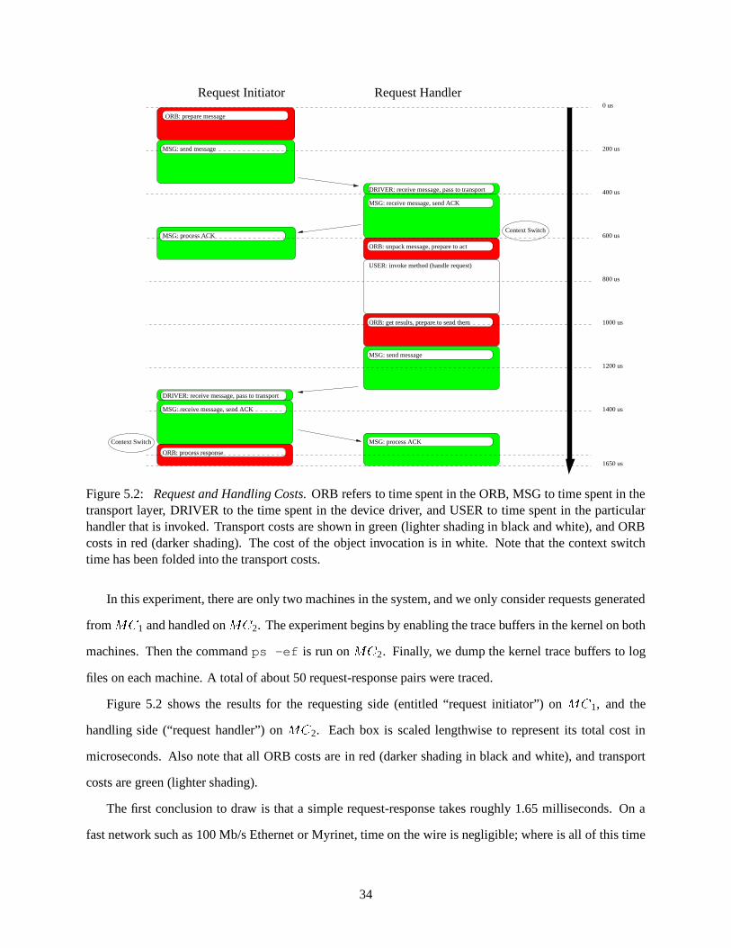
Figure 5.2: Request and Handling Costs. ORB refers to time spent in the ORB, MSG to time spent in thetransport layer, DRIVER to the time spent in the device driver, and USER to time spent in the particularhandler that is invoked. Transport costs are shown in green (lighter shading in black and white), and ORBcosts in red (darker shading). The cost of the object invocation is in white. Note that the context switchtime has been folded into the transport costs.

In this experiment, there are only two machines in the system, and we only consider requests generated

from��

1 and handled on� �

2. The experiment begins by enabling the trace buffers in the kernel on both

machines. Then the command ps -ef is run on� �

2. Finally, we dump the kernel trace buffers to log

files on each machine. A total of about 50 request-response pairs were traced.

Figure 5.2 shows the results for the requesting side (entitled “request initiator”) on��

1, and the

handling side (“request handler”) on� �

2. Each box is scaled lengthwise to represent its total cost in

microseconds. Also note that all ORB costs are in red (darker shading in black and white), and transport

costs are green (lighter shading).

The first conclusion to draw is that a simple request-response takes roughly 1.65 milliseconds. On a

fast network such as 100 Mb/s Ethernet or Myrinet, time on the wire is negligible; where is all of this time

34

going?

First, let us examine the request-initiating node. Before any messages are sent, the ORB spends roughly

150 � � preparing each request. At this point, the ORB hands the message to the transport layer. We can see

the cost of getting a message onto the wire is a costly 200 � � on average. Note that this high cost is mostly

due to expensive STREAMS-based utilities and locking protocols. After this, the request side waits for the

acknowledgment, which it soon receives, and then waits for the response to the request.

On the request-handle side, we can see what takes place as the request-initiator is waiting. First, the

packet is received by the driver, and passed up to the transport layer (50 � � ). This cost is an estimate, but since

all other time can be accounted for, is fairly accurate. The transport layer first sends the acknowledgment

back to the requesting side, strips off any transport headers, decides whom the packet is destined for (the

ORB), and then passes the message to the ORB. This takes 190-200 � � on average, again a costly sum.

After this, the first context switch occurs, and the ORB is given the message. After some interpretation

and set up, about 100 � � , the ORB finally performs the requested invocation. The cost of the invocation

is obviously application-specific, and in this case it is about 260 � � . Note that out of the 1.65 �� for a

request and response, this is the only work that is absolutely necessary. Thus, a request-response is currently

1650 ��260 ��

� 6 � 4, or about 6 times more expensive than the minimal possible cost.

After the invocation, the ORB prepares the response (analogous to the request side “prepare”) for another

150 � � or so, and sends a response back, again incurring the large transport overhead of about 200 � � .

Finally, the request side gets the response back, through the driver (50 � � estimated), through the transport

(200 � � ), and finally to the ORB, which interprets the message, places the results in the correct place and

finishes the request (another 100 � � ).

One last item to discuss is the latency of the network. For this experiment, 100-Mbit Ethernet was

employed. The time-on-the-wire for a 100-byte packet is only 8 � � . On any modern switch-based network,

latency across the wire is insignificant; clearly overhead is what matters in this domain.

5.2 Implications

As we can see from the micro-experiments of this section, the cost of each request-response is quite high.

There are two culprits in this high-latency hijinks: the transport layer and the ORB. The transport layer has

surprisingly large TCP-like overheads, with about 800 � � total in send and receive overhead, and another

35

100 � � in the drivers. Altogether, this accounts for roughly 1 �� of the total 1.65 �� involved in a simple

request-response, or 61% of the total time. Secondly, we see that ORB costs total to about 500 � � . While

this 30% of the time is only somewhat substantial now, we must compare it to the real cost of the remote

invocation, 250 � � . With an infinitely fast network protocol in place, the ORB would be responsible for

75% of all the time. Clearly, optimization work is desperately needed in both areas.

36

Chapter 6

Anatomy of a Message

Although previous data and discussion in this paper have focused on message sizes, destinations, and

request-response timings, this section brings the structure of each message under scrutiny. In doing so, we

resume use of our three workloads: make, web, and database. By examining the construction of each

message in detail, we hope to shed light on the potential areas a communication layer or network interface

should optimize for, and also attempt to understand how much overhead the object system requires, in terms

of bytes sent.

6.1 Buffer Chains

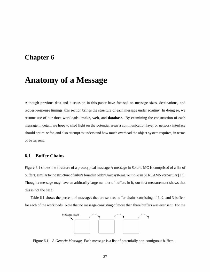
Figure 6.1 shows the structure of a prototypical message A message in Solaris MC is comprised of a list of

buffers, similar to the structure of mbufs found in older Unix systems, or mblks in STREAMS vernacular [27].

Though a message may have an arbitrarily large number of buffers in it, our first measurement shows that

this is not the case.

Table 6.1 shows the percent of messages that are sent as buffer chains consisting of 1, 2, and 3 buffers

for each of the workloads. Note that no message consisting of more than three buffers was ever sent. For the

Message Head

Figure 6.1: A Generic Message. Each message is a list of potentially non-contiguous buffers.

37

1 Buffer 2 Buffers 3 Buffersmake 0.6% 76.5% 22.9%web 0.7% 94.0% 5.3%database 0.0% 99.6% 0.4%

Table 6.1: Buffer Chains. The percent of messages sent as 1, 2, or 3 buffers in a chain across all workloads.Almost all messages were sent as 2 buffers in a chain. Each row totals to 100%.

make workload, 0% of messages are sent as a single buffer, 80% of messages consist of 2 buffers, and 20%

have 3 buffers. This imbalance increases across workloads, to 0/90/10 for the web workload, and 0/99/1 for

the database workload.

6.2 Protocol Overheads

Next, we give give buffer size distributions across all workloads. In Figure 6.2, we can see that the first

buffer in a chain is no bigger than 100 bytes, with about half of the first buffers 50 bytes in size. This buffer

is used by the underlying object system. The second buffer size distribution follows a pattern similar to the

message size distributions in Figures 4.3, 4.4, and 4.5. This buffer holds user payload, and not surprisingly

shows the greatest variation in size. Finally, the third buffer is occasionally used by the object system to

send object protocol information to another node. Across all workloads, this buffer is usually smaller than

the second buffer, never exceeding 512 bytes.

This leads to an obvious question: how much overhead as a percent of total bytes does the object system

require? Table 6.2 shows the breakdown for the three workloads.

The make and database workloads send many large messages. Since the payloads are large, the object

0%

20%

40%

60%

80%

100%

1 4 16 64 256 1 K 4 K 16 K

Per

cent

of M

essa

ges


Buffer Chain Distribution for Make

Buffer 1Buffer 2Buffer 3

0%

20%

40%

60%

80%

100%

1 4 16 64 256 1 K 4 K 16 K

Per

cent

of M

essa

ges


Buffer Chain Distribution for WWW


0%

20%

40%

60%

80%

100%

1 4 16 64 256 1 K 4 K 16 K

Per

cent

of M

essa

ges


Buffer Chain Distribution for Database


Figure 6.2: Buffer Chain Sizes. These figures plot the distribution of sizes for each buffer of a message.Note that the bulk of the data is sent in the second buffer chain.

38

1st Buffer 2nd Buffer 3rd Buffermake 8.4% 89.2% 2.4%web 33.9% 64.9% 1.2%database 5.9% 94.0% 0.1%

Table 6.2: Object Protocol Overheads. The table shows what percentage of bytes were sent in each bufferin the buffer chain. Each row totals to 100%.

overheads are relatively small. With the web workload, however, we can see that the overheads are more

substantial, though as we saw in Figure 6.2, they are not absolutely any larger. In this workload, because

the largest payloads are fairly small, about 1500 bytes, and there are many small messages sent, the object

overhead is a noticeable fraction.

6.3 Implications

In this section, we inspected the structure of a Solaris MC message. The first and third buffers are used by

the object system for protocol information, while the second is the payload of the Solaris MC programmer.

Messages are a chain of usually 2 or 3 non-contiguous buffers. The size distribution of the distinct buffers is

radically different: the first and third buffer are small, while the second buffer ranges from small (a hundred

bytes) to quite large (up to 8 KB for the make workload).

The existence of buffer chains implies that the message layer must either support a “gather” interface, or

perform an extra copy and buffer allocation before sending the data. However, a gathering interface is not

present in some of today’s fast messaging layers [17, 33]. The only alternative is to significantly restructure

the MC code to always allocate extra space within each object in anticipation of the object system’s demands.

The gather cost is directly proportional to memory copy costs, plus the the cost of buffer allocation. If this

is substantial, a restructuring of the code may be worth pursuing, since not much use is made of the buffer

chains. Finally, though each message requires something like 50-100 bytes of object header information,

we have seen that for the web workload, 40% of all bytes transferred are for the ORB.

39

Chapter 7

Conclusions and Future Work

In this paper, we have measured the performance of various workloads on a prototype cluster operating

system, Solaris MC. Our measurements have revealed interesting results for both message-layer design as

well as from a distributed system design perspective.

From a systems perspective, some key Solaris MC design decisions could adversely affect performance.

For example, the use of a non-striped file system could lead to bottlenecks occurring around certain disks

in the system. Further, this node usually sent the most data to other nodes in the system. Other global

services such as the network port name-space manager could suffer from similar bottlenecks if they are not

distributed. Lastly, since nodes that house disks are often sending large messages, optimizing the path from

disk to network may prove worthwhile.

With message layer design in mind, we find that message traffic is highly workload dependent. The

cluster can be used as a compute server, a database engine, or even a web server, and each of these scenarios

will cause the system to behave quite differently. Performance optimization of an MC system clearly

depends on its intended use. However, it is clear that support for medium-sized messages is important for

all workloads, since 80% of all messages across all workloads were in the range of 68 to 256 bytes.

After instrumenting the object subsystem, we have seen that the prototype implementation of Solaris MC

suffers from unusually high request-response times. Most of this can be attributed to the slow STREAMS-

based transport, which contributes to high overhead as well as high latency. The current cost of the object

infrastructure is also quite high; thus, in an ideal case where the transport layer is fast, the overhead of the

object system becomes quite significant.

Finally, support for a gathering interface could be of some limited benefit. Since the object system often

40

attaches its own header to each request as a separate buffer, some implementation effort at that level could

potentially remove any such need.

In the future, much remains to be examined. From the perspective of the workloads, both the web and

database workloads could be more realistic. For example, the web workload could be trace-driven from

the usage patterns of a popular web-site, and also make use of a better web server such as the netscape

server. The database workload would be much better off with more disks, and also with standard database

benchmarks such as TPC-C and TPC-D.

Since the system is currently evolving, repeating the measurements will yield insight as to which

problems have been solved, and which persist. It is clear that a fast, lightweight transport could be of

great use, and this avenue is currently under exploration. After this is in place, tuning of the ORB will be

necessary, the costs are spread all along the whole ORB code path, and early measurements have indicated

that memory allocation needs to be improved. In both cases, low overhead will significantly improve overall

system performance. In that light, one could view this report as a prototype of a continued series of refined

evaluations.

41

Bibliography

[1] T. Anderson, M. Dahlin, J. Neefe, D. Patterson, and R. Wang. Serverless Network File Systems. InFifteenth ACM Symposium on Operating Systems Principles, pages 109–26, Copper Mountain Resort,CO, USA, Dec 1995.

[2] T. E. Anderson, S. S. Owicki, J. Saxe, and C. Thacker. High-speed Switch Scheduling for Local-AreaNetworks. ACM Transactions on Computer Systems, 11(4):319–352, Nov 1993.

[3] M. Baker, J. Hartman, M. Kupfer, K. Shirriff, and J. Ousterhout. Measurements of a DistributedFile System. In Proceedings of the Thirteenth Symposium on Operating Systems Principles, pages198–212, Pacific Grove, CA, USA, oct 1991.

[4] F. Baskett and J. H. Howard. Task communicaton in DEMOS. In Proceedings of the ACM Symposiumon Operating System Principles, pages 23–32, Reading, MA, USA, 1977.

[5] J. Bernebeu, V. Matena, and Y. Khalidi. Extending a Traditional OS Using Object-Oriented Techniques.To appear in COOTS 96, 1996.

[6] N. Boden, D. Cohen, R. Felderman, A. Kulawik, and C. Seitz. Myrinet: A Gigabit-per-second LocalArea Network. IEEE Micro, 15(1):29–36, Feb 1995.

[7] D. R. Cheriton. VMTP: A Transport Protocol for the Next Generation of Communication Systems. InProceedings of ACM SIGCOMM, pages 406–415, Stowe, VT, Aug. 1986.

[8] D. R. Cheriton. The V Distributed System. Communications of the ACM, 31(3):12–28, Mar. 1988.

[9] D. R. Cheriton and C. L. Williamson. Network Measurement of the VMTP Request-Response Protocolin the V Distributed System. In Proceedings of ACM SIGCOMM, pages 216–225, Stowe, VT, Aug.1987.

[10] J. Chu. Zero-copy TCP in Solaris. In Proceedings of the 1996 Usenix Technical Conference, pages253–64, San Diego, CA, USA, Jan. 1996.

[11] F. Douglis, J. K. Ousterhout, M. F. Kaashoek, and A. S. Tanenbaum. A Comparison of Two DistributedSystems: Amoeba and Sprite. Computing Systems, 4(4):353–383, Fall 1991.

[12] R. Finkel and M. Scott. Experience with Charlotte: Simplicity and function in a distributed operatingsystem. IEEE Transactions on Software Engineering, 15:676–686, June 1989.

[13] J. Hartman and J. Ousterhout. The Zebra Striped Network File System. In Proceedings of the FourteenthSymposium on Operating Systems Principles, pages 29–43, Ashville, NC, USA, Dec. 1993.

42

[14] M. F. Kaashoek, R. van Renesse, H. van Staveren, and A. S. Tanenbaum. FLIP: an InternetworkProtocol for Supporting Distributed Systems. Technical report, Department of Mathematics andComputer Science, Vrije Universiteit, July 1991.

[15] Y. Khalidi, J. Bernebeu, V. Matena, K. Shirriff, and M. Thadani. Solaris MC: A Multi-Computer OS.In 1996 Winter Usenix, pages 205–218. USENIX, Jan. 1996.

[16] Y. A. Khalidi and M. N. Nelson. Extensible File Systems in Spring. In Proceedings of the FourteenthSymposium on Operating Systems Principles, Ashville, NC, USA, Dec 1993.

[17] A. M. Mainwaring. Active Message Application Programming Interface and Communication Subsys-tem Organization. Master’s thesis, University of California, Berkeley, 1995.

[18] R. P. Martin. HPAM: An Active Message Layer for a Network of Workstations. In Proceedings of HotInterconnects II, July 1994.

[19] V. Matena, J. Bernabeu, and Y. A. Khalidi. High Availability Support in Solaris MC. Technical report,Sun Microsystem Laboratories, Moutain View, CA, To appear in 1996.

[20] L. McVoy and C. Staelin. lmbench: Portable Tools for Performance Analysis. In Proceedings of the1996 Winter USENIX, Jan. 1996.

[21] J. Mogul, R. Rashid, and M. Accetta. The Packet Filter: An Efficient Mechanism For User-LevelNetwork Code. In Proceedings of the Eleventh Symposium on Operating Systems Principles, pages39–51, Austin, TX, USA, nov 1987.

[22] S. J. Mullender, G. V. Rossum, A. S. Tanenbaum, R. V. Renesse, and H. van Staveren. Amoeba – ADistributed Operating System for the 1990’s. IEEE Computer Magazine, 33(12):46–63, May 1990.

[23] NCSA HTTPd Development Team. NCSA HTTPd. http://hoohoo.ncsa.uiuc.edu, Apr. 1996.

[24] J. K. Ousterhout, A. R. Cherenson, F. Douglis, M. N. Nelson, and B. B. Welch. The Sprite NetworkOperating System. IEEE Computer, 21(2):23–36, Feb. 1988.

[25] G. J. Popek and B. J. Walker, editors. The LOCUS Distributed System Architecture, pages 73–89.Computer Systems Series. The MIT Press, 1985.

[26] D. M. Ritchie and K. Thompson. The UNIX Time-Sharing System. Communications of the ACM,17(7):365–75, July 1974.

[27] D. Schmidt and T. Suda. Transport System Architecture Services For High-performance Communica-tions Systems. IEEE Journal on Selected Areas in Communications, 11(4):489–506, May 1993.

[28] SPEC Design Committee. SPECweb. http://www.specbench.org/osg/web/, Apr. 1996.

[29] SunSoft Technical Writers. TNF Manual Page. Solaris AnswerBook, 1996.

[30] F. Tibbitts. CORBA: A Common Touch For Distributed Applications. Data Communications Inter-national, 24(7):71–5, May 1995.

[31] R. van Rennesse and A. Tanenbaum. Amoeba: The World’s Fastest Operating System. In OperatingSystems Review, Dec 1989.

43

[32] T. von Eicken, A. Basu, V. Buch, and W. Vogels. U-net: A user-level network interface for paralleland distributed computing. In Proceedings of the Fifteenth ACM Symposium on Operating SystemsPrinciples, pages 40–53, Copper Mountain Resort, CO, USA, 1995.

[33] T. von Eicken, D. E. Culler, S. C. Goldstein, and K. E. Schauser. Active Messages: a Mechanismfor Integrated Communication and Computation. In Proc. of the 19th International Symposium onComputer Architecture, pages 256–266, Gold Coast, Australia, May 1992.

[34] B. Welch. A Comparison of Three Distributed File System Architectures: Vnode, Sprite, and Plan 9.Computing Systems, 7(2):175–99, Spring 1994.

44

communication behavior of a distributed operating...

Documents