communication-aware motion planning in mobile networks
TRANSCRIPT

University of New MexicoUNM Digital Repository
Electrical and Computer Engineering ETDs Engineering ETDs
1-31-2013
Communication-aware motion planning in mobilenetworksAlireza Ghaffarkhah
Follow this and additional works at: https://digitalrepository.unm.edu/ece_etds
This Dissertation is brought to you for free and open access by the Engineering ETDs at UNM Digital Repository. It has been accepted for inclusion inElectrical and Computer Engineering ETDs by an authorized administrator of UNM Digital Repository. For more information, please [email protected].
Recommended CitationGhaffarkhah, Alireza. "Communication-aware motion planning in mobile networks." (2013). https://digitalrepository.unm.edu/ece_etds/96

Candidate
Department This dissertation is approved, and it is acceptable in quality and form for publication: Approved by the Dissertation Committee: , Chairperson
Alireza Ghaffarkhah
Electrical and Computer Engineering
Yasamin Mostofi
Chaouki Abdallah
Rafael Fierro
Lydia Tapia
i

Communication-Aware Motion Planningin Mobile Networks
by
Alireza Ghaffarkhah
B.S., Sharif University of Technology, 2005
M.S., Sharif University of Technology, 2007
DISSERTATION
Submitted in Partial Fulfillment of the
Requirements for the Degree of
Doctor of Philosophy
Engineering
The University of New Mexico
Albuquerque, New Mexico
December 2012

c©2012, Alireza Ghaffarkhah
iii

Dedication
To my mother and father
iv

Acknowledgments
First and foremost, I would like to thank my advisor Prof. Yasamin Mostofi. She isa great teacher, an excellent mentor, an intelligent researcher and most importantlya trustworthy friend. I learnt a great deal from our numerous technical discussions.She is indeed the most hardworking person I have ever known and I will alwaysadmire her professionalism, enthusiasm for new ideas and dedication to research.
I would like to thank Prof. Chaouki Abdallah, Prof. Rafael Fierro and Prof.Lydia Tapia for serving on my dissertation committee. They are among the mostknowledgeable people I have had the pleasure to meet at UNM. Prof. Abdallah hasalways been so supportive of me and I need to thank him for agreeing to be on mydissertation committee despite his extremely busy schedule as the Interim Provostat UNM. My special thanks also go to Prof. Fierro for always being so nice andhelpful and for letting us use his lab during our experiments. Without his help doingexperiments could be very painful. And I need to thank Prof. Tapia who agreed tobe on my committee on short notice.
I would like to thank all the members of our research group at the CooperativeNetwork Lab at UNM, specially Mehrzad Malmirchegini, Alejandro Gonzalez-Ruizand Yuan Yan, for being such great friends.
Finally, I want to thank my family, specially my mother Mahnaz and fatherMehrdad, for their infinite love and support. To them, I owe everything.
v

Communication-Aware Motion Planningin Mobile Networks
by
Alireza Ghaffarkhah
B.S., Sharif University of Technology, 2005
M.S., Sharif University of Technology, 2007
Ph.D., University of New Mexico, 2012
Abstract
Over the past few years, considerable progress has been made in the area of networked
robotic systems and mobile sensor networks. The vision of a mobile sensor network
cooperatively learning and adapting in harsh unknown environments to achieve a
common goal is closer than ever. In addition to sensing, communication plays a key
role in the overall performance of a mobile network, as nodes need to cooperate to
achieve their tasks and thus have to communicate vital information in environments
that are typically challenging for communication. Therefore, in order to realize the
full potentials of such networks, an integrative approach to sensing (information
gathering), communication (information exchange), and motion planning is needed,
such that each mobile sensor considers the impact of its motion decisions on both
sensing and communication, and optimizes its trajectory accordingly. This is the
main motivation for this dissertation.
This dissertation focuses on communication-aware motion planning of mobile net-
works in the presence of realistic communication channels that experience path loss,
vi

shadowing and multipath fading. This is a challenging multi-disciplinary task. It
requires an assessment of wireless link qualities at places that are not yet visited by
the mobile sensors as well as a proper co-optimization of sensing, communication
and navigation objectives, such that each mobile sensor chooses a trajectory that
provides the best balance between its sensing and communication, while satisfying
the constraints on its connectivity, motion and energy consumption. While some
trajectories allow the mobile sensors to sense efficiently, they may not result in a
good communication. On the other hand, trajectories that optimize communica-
tion may result in poor sensing. The main contribution of this dissertation is then
to address these challenges by proposing a new paradigm for communication-aware
motion planning in mobile networks. We consider three examples from networked
robotics and mobile sensor network literature: target tracking, surveillance and dy-
namic coverage. For these examples, we show how probabilistic assessment of the
channel can be used to integrate sensing, communication and navigation objectives
when planning the motion in order to guarantee satisfactory performance of the
network in realistic communication settings. Specifically, we characterize the perfor-
mance of the proposed framework mathematically and unveil new and considerably
more efficient system behaviors. Finally, since multipath fading cannot be assessed,
proper strategies are needed to increase the robustness of the network to multipath
fading and other modeling/channel assessment errors. We further devise such ro-
bustness strategies in the context of our communication-aware surveillance scenario.
Overall, our results show the superior performance of the proposed motion planning
approaches in realistic fading environments and provide an in-depth understanding
of the underlying design trade-off space.
vii

Contents
List of Figures xiv
List of Tables xxiv
1 Introduction 1
1.1 Contributions of the Dissertation . . . . . . . . . . . . . . . . . . . . 3
1.2 Related Work . . . . . . . . . . . . . . . . . . . . . . . . . . . . . . . 9
1.2.1 Probabilistic Assessment of Wireless Channels and Motion Plan-
ning for Improving Channel Prediction Quality . . . . . . . . 10
1.2.2 Target Tracking Using Mobile Networks . . . . . . . . . . . . 10
1.2.3 Surveillance, Exploration and Field Estimation Using Mobile
Networks . . . . . . . . . . . . . . . . . . . . . . . . . . . . . 12
1.2.4 Dynamic Coverage of Time-Varying Environments Using Mo-
bile Networks . . . . . . . . . . . . . . . . . . . . . . . . . . . 13
1.3 Notations . . . . . . . . . . . . . . . . . . . . . . . . . . . . . . . . . 15
2 Probabilistic Assessment of Wireless Channels and Motion Plan-
viii

Contents
ning for Improving Channel Prediction Quality 16
2.1 Probabilistic Modeling of Wireless Channels . . . . . . . . . . . . . . 18
2.2 Probabilistic Channel Assessment Based on a Small Number of Chan-
nel Measurements . . . . . . . . . . . . . . . . . . . . . . . . . . . . . 22
2.3 Sensitivity of Channel Assessment to the Estimation Error of the
Channel Parameters . . . . . . . . . . . . . . . . . . . . . . . . . . . 29
2.4 Motion Planning for Improving Wireless Channel Assessment in Mo-
bile Networks . . . . . . . . . . . . . . . . . . . . . . . . . . . . . . . 31
2.4.1 Motion Planning for Improving the Estimation of the Under-
lying Channel Parameters . . . . . . . . . . . . . . . . . . . . 32
2.4.2 Motion Planning for Reducing the Channel Assessment Uncer-
tainty . . . . . . . . . . . . . . . . . . . . . . . . . . . . . . . 36
2.5 Summary . . . . . . . . . . . . . . . . . . . . . . . . . . . . . . . . . 39
3 Communication-Aware Target Tracking Using Mobile Networks 41
3.1 Problem Formulation . . . . . . . . . . . . . . . . . . . . . . . . . . . 43
3.2 Communication-Aware Target Tracking Using Probabilistic Assess-
ment of Wireless Channels . . . . . . . . . . . . . . . . . . . . . . . . 46
3.2.1 Discussion on Local Extrema Avoidance . . . . . . . . . . . . 51
3.3 Simulation and Experimental Results . . . . . . . . . . . . . . . . . . 52
3.4 Summary . . . . . . . . . . . . . . . . . . . . . . . . . . . . . . . . . 55
4 Communication-Aware Surveillance Using Mobile Networks 57
ix

Contents
4.1 Problem Formulation . . . . . . . . . . . . . . . . . . . . . . . . . . . 61
4.1.1 Sensing and Dynamical Models of the Mobile Sensors . . . . . 63
4.1.2 The Communication Model and Probabilistic Characterization
of Wireless Links . . . . . . . . . . . . . . . . . . . . . . . . . 64
4.2 Multi-Sensor Surveillance in the Presence of Fading Channels . . . . . 65
4.2.1 Optimal Sequential Detection at Mobile Sensors . . . . . . . . 66
4.2.2 Optimal Detection at the Remote Station . . . . . . . . . . . 68
4.2.3 Mathematical Characterization of the Performance at the Re-
mote Station . . . . . . . . . . . . . . . . . . . . . . . . . . . 70
4.2.4 Chernoff Bound On the Probability of Error at the Remote
Station . . . . . . . . . . . . . . . . . . . . . . . . . . . . . . . 73
4.3 Motion Planning and Power Management Strategies for Minimizing
the Detection Error Probability at the Remote Station . . . . . . . . 74
4.3.1 Communication-Constrained Motion Planning . . . . . . . . . 76
4.3.2 Hybrid Motion Planning . . . . . . . . . . . . . . . . . . . . . 80
4.4 Further Robustness to Multipath Fading and other Channel Assess-
ment/Modeling Errors . . . . . . . . . . . . . . . . . . . . . . . . . . 84
4.4.1 Adaptive Transmit Power and Packet Dropping Threshold for
Increasing the Robustness to Multipath Fading . . . . . . . . 85
4.4.2 Jittery Movements for Increasing the Probability of Connec-
tivity in the Presence of Large Multipath Fading . . . . . . . . 87
4.5 Performance Analysis of the Proposed Motion Planning Strategies . . 88
x

Contents
4.6 Simulation and Experimental Results . . . . . . . . . . . . . . . . . . 92
4.7 Summary . . . . . . . . . . . . . . . . . . . . . . . . . . . . . . . . . 99
5 Communication-Aware Dynamic Coverage of Time-Varying Envi-
ronments Using Mobile Networks 103
5.1 System Modeling . . . . . . . . . . . . . . . . . . . . . . . . . . . . . 109
5.1.1 Communication Model of the Mobile Agents . . . . . . . . . . 111
5.1.2 Energy Consumption Model of the Mobile Agents . . . . . . . 113
5.2 Dynamic Coverage of Time-Varying Environments in the Communication-
Intensive Case . . . . . . . . . . . . . . . . . . . . . . . . . . . . . . . 115
5.2.1 Problem Formulation . . . . . . . . . . . . . . . . . . . . . . . 115
5.2.2 Optimal Solution of the Dynamic Coverage Problem in the
Communication-Intensive Case – Case of Known Channel Pow-
ers at the POIs . . . . . . . . . . . . . . . . . . . . . . . . . . 119
5.2.3 Optimal Solution of the Dynamic Coverage Problem in the
Communication-Intensive Case – Case of Unknown Stochastic
Channel Powers at the POIs . . . . . . . . . . . . . . . . . . . 126
5.2.4 Probabilistic Analysis of the Dynamic Coverage Problem in
the Communication-Intensive Case . . . . . . . . . . . . . . . 129
5.3 Dynamic Coverage of Time-Varying Environments in the Communication-
Efficient Case . . . . . . . . . . . . . . . . . . . . . . . . . . . . . . . 136
5.3.1 Problem Formulation . . . . . . . . . . . . . . . . . . . . . . . 136
xi

Contents
5.3.2 Optimal Solution of the Dynamic Coverage Problem in the
Communication-Efficient Case – Case of Known Channel Pow-
ers at the POIs . . . . . . . . . . . . . . . . . . . . . . . . . . 138
5.3.3 Optimal Solution of the Dynamic Coverage Problem in the
Communication-Efficient Case – Case of Unknown Stochastic
Channel Powers at the POIs . . . . . . . . . . . . . . . . . . . 143
5.3.4 Probabilistic Analysis of the Dynamic Coverage Problem in
the Communication-Efficient Case . . . . . . . . . . . . . . . . 144
5.4 Simulation Results . . . . . . . . . . . . . . . . . . . . . . . . . . . . 147
5.5 Further Extension of the Dynamic Coverage Problem . . . . . . . . . 161
5.5.1 Motion Model . . . . . . . . . . . . . . . . . . . . . . . . . . . 162
5.5.2 Communication Model . . . . . . . . . . . . . . . . . . . . . . 164
5.6 Extended Dynamic Coverage of Time-Varying Environments . . . . . 165
5.6.1 Problem Formulation . . . . . . . . . . . . . . . . . . . . . . . 166
5.6.2 Optimal Solution of the Dynamic Coverage in Case of Non-
zero Ranges and Adaptive Velocities, Transmission Powers and
Transmission Rates . . . . . . . . . . . . . . . . . . . . . . . 168
5.6.3 Mathematical Analysis and Special Cases . . . . . . . . . . . . 172
5.7 Simulation Results for the Extended Dynamic Coverage Problem . . . 179
5.8 Summary . . . . . . . . . . . . . . . . . . . . . . . . . . . . . . . . . 186
6 Conclusions and Further Extensions 193
xii

Contents
References 198
xiii

List of Figures
2.1 Underlying dynamics of the received signal power across a route in the
basement of the ECE building at UNM. d is the distance to the transmitter. 17
2.2 A simulated channel (left) and the mean of its probability distribution
(GdB,k,t(q) in Theorem 2.2.2) (right). The channel is simulated using
our probabilistic channel simulator, with the following parameters: θ =
[−10 2.0]T, ϑ = 4.0 dB, β = 20 m and ω = 1.13 dB (corresponding to
a Rician distribution with parameter Kr = 30). The total number of a
priori gathered channel samples is 515, which is 0.5% of the grid size (the
grid is 320× 320). . . . . . . . . . . . . . . . . . . . . . . . . . . . . . 27
2.3 The received signal strength across a street in downtown San Francisco
along with its reconstructed version (left) and an indoor received signal
strength along a route in the basement of the ECE building at UNM and
its reconstruction (right). The outdoor data is courtesy of Mark Smith.
In both cases, the reconstruction is based on only 5% a priori channel
measurements. . . . . . . . . . . . . . . . . . . . . . . . . . . . . . . 28
2.4 Channel prediction quality for the outdoor (left) and indoor (right) chan-
nels of Fig. 2.3, as a function of the percentage of the measurements
gathered. . . . . . . . . . . . . . . . . . . . . . . . . . . . . . . . . . 28
xiv

List of Figures
2.5 Performance of the channel assessment framework in a cooperative channel
assessment scenario – trajectories of the mobile sensors (left), a snapshot
of the true channel power map (middle) and the average of its probabilistic
reconstruction using our framework (GdB,k,t(q) in Theorem 2.2.2) (right).
The empty circles and the filled ones in the left figure show the initial and
final positions of the mobile sensors respectively. The original channel is
the same as in Fig. 2.2. The total number of gathered samples is 350,
which is 0.34% of the grid size. . . . . . . . . . . . . . . . . . . . . . . 29
2.6 Spatial average of ∆2k,t(q), as a function of the % of estimation error in
θk,t, ϑ2k,t, βk,t and ωk,t. . . . . . . . . . . . . . . . . . . . . . . . . . . 31
2.7 Trajectory of a mobile mobile sensor in communication-aware motion
planning for improving path loss parameter estimation in an indoor envi-
ronment (left) and the corresponding normalized estimation error variance
(right). The empty circle and the filled one in the left figure denote the
initial and final positions of the mobile sensor. . . . . . . . . . . . . . . 36
2.8 Trajectory of a mobile mobile sensor in communication-aware motion
planning for reducing channel assessment uncertainty in an outdoor envi-
ronment (left) and the corresponding ANMSE (right). The empty circle
and the filled one in the left figure denote the initial and final positions of
the mobile sensor. . . . . . . . . . . . . . . . . . . . . . . . . . . . . . 38
2.9 Snapshots of the channel assessment error variance over the workspace
(top left for t = 0, top right for t = 50, bottom left for t = 100 and
bottom right for t = 200) . . . . . . . . . . . . . . . . . . . . . . . . . 39
3.1 A schematic of the networked target tracking operation considered in this
chapter. . . . . . . . . . . . . . . . . . . . . . . . . . . . . . . . . . . 42
xv

List of Figures
3.2 Performance of the proposed communication-aware target tracking frame-
work in an outdoor environment – The left figure shows the trajectories of
the mobile sensors and the target. The solid magenta and dashed red lines
correspond to the trajectory of the mobile sensors in communication-aware
and communication-unaware cases respectively, while the yellow dash-
dot line represents the trajectory of the target. The empty circles/box
and the filled ones show the initial and final positions of the mobile
sensors/target respectively. The right figure compares the performance
of four approaches, with different levels of communication-awareness, in
terms estimation error covariance at the remote station (RS). . . . . . . 54
3.3 Performance of the proposed communication-aware target tracking frame-
work in an indoor environment (basement of the Electrical and Computer
Engineering building at the University of New Mexico) – The left figure
shows the trajectories of the mobile sensor and the target (see the expla-
nation of Fig. 3.2). The right figure compares the performance of four
approaches, with different levels of communication-awareness, in terms
estimation error covariance at the remote station (RS). . . . . . . . . . . 55
4.1 A schematic of the networked surveillance operation considered in this
chapter. . . . . . . . . . . . . . . . . . . . . . . . . . . . . . . . . . . 58
4.2 Illustration of the proposed communication-constrained motion planning
approach. . . . . . . . . . . . . . . . . . . . . . . . . . . . . . . . . . 80
4.3 Illustration of the proposed hybrid motion planning approach. . . . . . . 84
4.4 Illustration of the proposed probabilistic channel assessment framework
and robustness techniques. . . . . . . . . . . . . . . . . . . . . . . . . 85
xvi

List of Figures
4.5 Trajectories of three mobile sensors for communication-constrained (left)
and hybrid (right) cases, with fixed TX powers. The red, magenta and
green lines correspond to the trajectories of the Mobile Sensor #1, Mobile
Sensor #2 and Mobile Sensor #3, respectively. The empty boxes and the
filled ones denote the initial and final positions respectively. The location
of the remote station is denoted on the top left corner of the figures. See
the pdf file for more visual clarity. . . . . . . . . . . . . . . . . . . . . 94
4.6 Impact of the adaptive TX power on connectivity regions. Time-varying
connectivity regions (white areas) in communication-constrained (top row)
and hybrid (bottom row) cases are shown for one of the mobile sensors
of Fig. 4.5, at time steps t = 15, t = 25, t = 35 and t = 45 (from left to
right). The communication channel is taken to be the same as the one
used in Fig. 4.5. Empty boxes and filled ones denote the initial and final
positions respectively. See the pdf file for more visual clarity. . . . . . . 95
4.7 Average of the detection error probability at the remote station (RS) as
a function of (left) the given operation time (T ) and (right) time step (t)
for communication-constrained and hybrid approaches. TX power is not
adaptive in this case. . . . . . . . . . . . . . . . . . . . . . . . . . . . 97
4.8 Communication and sensing trade-offs in a networked surveillance sce-
nario. The figure shows average of the final detection error probability at
the remote station (RS), averaged over the space and channel distribution,
as a function of SNRTH, for two cases of T = 10 (left) and T = 50 (right). 98
xvii

List of Figures
4.9 Performance of the proposed communication-aware surveillance frame-
work using real channel measurements in an indoor environment (base-
ment of the Electrical and Computer Engineering building at UNM).
The left and right figures show the trajectory of the mobile sensor in
the communication-constrained and hybrid approaches respectively, where
the true connectivity map to the remote station is superimposed on the
blueprint of the basement. . . . . . . . . . . . . . . . . . . . . . . . . 100
4.10 The resulting average of the detection error probability at the remote
station (RS), as a function of time step t, for the indoor environment of
Fig. 4.9. . . . . . . . . . . . . . . . . . . . . . . . . . . . . . . . . . . 101
4.11 The picture of the Pioneer 3-AT robot, equipped with directional and
omni-directional antennas, used for channel measurements in the indoor
surveillance scenario of Fig. 4.9. Only omni-directional channel measure-
ment were used in this example. . . . . . . . . . . . . . . . . . . . . . 102
4.12 Comparison of different motion planning approaches, based on the level
of communication and sensing awareness and its impact on the overall
performance. . . . . . . . . . . . . . . . . . . . . . . . . . . . . . . . 102
5.1 Dynamic coverage of a time-varying environment using a team of mobile
agents. Ψi(t) is the quantity of interest at the ith POI that needs to be
kept bounded by periodically visiting the POI. . . . . . . . . . . . . . . 105
5.2 A sample plot of Ψi(t) at the remote station in the communication-
intensive case, for one of the POIs, after optimizing the dynamic coverage
operation using the MILP of Program 1. The left figure corresponds to
the case where ∆k > 0 (robust dynamic coverage with positive stability
margin) and the right one corresponds to the case where ∆k = 0 (zero
stability margin). . . . . . . . . . . . . . . . . . . . . . . . . . . . . . 126
xviii

List of Figures
5.3 Sample plots of Ψi(t) and Φi(t) in the communication-efficient case for
one of the POIs after optimizing the dynamic coverage operation using
the MILP of Program 2. The left figure corresponds to the case where
∆k > 0 (robust dynamic coverage with positive stability margin) and the
right figure corresponds to the case where ∆k = 0 (zero stability margin). 142
5.4 The 3D plot of the channel power G(q) over the workspace of Fig. 5.5. . . 149
5.5 The optimal trajectories of the mobile agents in the communication-intensive
(left) and communication-efficient (right) cases for the case of known chan-
nel. The solid red, dashed blue and dot-dashed green lines correspond to
the trajectories of Agent 1, 2 and 3 respectively. The location of the
remote station is denoted at the top left corner of the figures. The opti-
mal communication points for each mobile agent in the communication-
efficient case is also specified by a circle in the right figure. . . . . . . . . 152
5.6 The plot of Ψi(t) at the remote station for POI #4 in Fig. 5.5 in communication-
intensive (left) and communication-efficient (right) cases. In the communication-
efficient case, the plot of Φi(t) at the mobile agent is also provided. . . . 153
5.7 The comparison of the estimated and real channel powers at the POIs
(left) and the optimal trajectories of one mobile agent in both communication-
intensive and communication-efficient cases and for the case of unknown
channel powers (right). The location of the remote station is denoted at
the top left corner of the right figure. The optimal communication point
for the mobile agent in the communication-efficient case is also specified
by a circle in the right figure. It can be seen that the optimal trajectory
is the Hamiltonian cycle over the set of POIs. . . . . . . . . . . . . . . 154
xix

List of Figures
5.8 The plots of Ψi(t) at the remote station for POI #4 (left) and POI #10
(right) in Fig. 5.7. These figures compare the time evolution of Ψi(t)
in communication-intensive, communication-efficient and communication-
unaware cases. . . . . . . . . . . . . . . . . . . . . . . . . . . . . . . 156
5.9 Positions of the POIs superimposed on the connectivity map to the remote
station, assuming that the fixed transmission power 1m
∑i∈V Γ(qi, χ) is
used in the communication-unaware case. The disconnected POIs are
circled on the figure. . . . . . . . . . . . . . . . . . . . . . . . . . . . 157
5.10 The percentage of the POIs that can be covered by the mobile agent of
Fig. 5.7 in the communication-intensive case (left), the probability of con-
nectivity of the optimal transmission point in the communication-efficient
case (middle), and the total optimal communication energy (right) as a
function of multipath power. . . . . . . . . . . . . . . . . . . . . . . . 159
5.11 Two sample channels with ω = 0.8730 dB (left) and ω = 5.0941 dB (right).
The path loss and shadowing components of both channels are the same
as in Fig. 5.4 . . . . . . . . . . . . . . . . . . . . . . . . . . . . . . . 159
5.12 The actual and theoretical average minimum total energy consumed in
each period to cover a set of POIs, as a function of the number of POIs. . 160
5.13 The actual and theoretical average minimum communication energy con-
sumed in each period to cover a set of POIs as a function of the number of
POIs, in the communication-intensive (left) and communication-efficient
(right) cases. . . . . . . . . . . . . . . . . . . . . . . . . . . . . . . . 161
5.14 The 3D plot of the channel power G(q) over the workspace. . . . . . . . 180
xx

List of Figures
5.15 The optimal trajectory of the mobile agent in case Type I constraints
in (5.69) are used for the total transmission time in each segment. The
location of the remote station is denoted at the center of the figures.
The green parts of the trajectory in the left figure show the segments
where the mobile agent slows down, i.e., the segments where ∗i,j,k > v−1max.
The green parts in the right figure also show the segments where the
information bits are transmitted to the remote station, i.e., the segments
where∑nr
ℓ=1 τ∗i,j,k,ℓ > 0. . . . . . . . . . . . . . . . . . . . . . . . . . . 181
5.16 The velocity profile (left) and the transmission time profile (right) of the
mobile agent along the optimal trajectory of Fig. 5.15. We have specified
the paths between any two POIs along the trajectory on both figures. . . 182
5.17 The plots of∑nr
ℓ=1 τ∗i,j,k,ℓ
(2RTX,ℓ − 1
)(top) and Gi,j,k (as a measure of the
predicted channel quality) (bottom) along the optimal trajectory of Fig.
5.15. . . . . . . . . . . . . . . . . . . . . . . . . . . . . . . . . . . . . 183
5.18 The optimal trajectory of the mobile agent in case Type II constraints
in (5.70) are used for the total transmission time in each segment. The
location of the remote station is denoted at the center of the figures.
The green parts of the trajectory in the left figure show the segments
where the mobile agent slows down, i.e., the segments where ∗i,j,k > v−1max.
The green parts in the right figure also show the segments where the
information bits are transmitted to the remote station, i.e., the segments
where∑nr
ℓ=1 τ∗i,j,k,ℓ > 0. . . . . . . . . . . . . . . . . . . . . . . . . . . 184
5.19 The velocity profile (left) and the transmission time profile (right) of the
mobile agent along the optimal trajectory of Fig. 5.18. We have specified
the paths between any two POIs along the trajectory in both figures. . . 185
xxi

List of Figures
5.20 The plots of∑nr
ℓ=1 τ∗i,j,k,ℓ
(2RTX,ℓ − 1
)(top) and Gi,j,k (as a measure of the
predicted channel quality) (bottom) along the optimal trajectory of Fig.
5.18. . . . . . . . . . . . . . . . . . . . . . . . . . . . . . . . . . . . . 186
5.21 The optimal trajectory of the mobile agent in case Type I constraints
in (5.69) are used for the total transmission time in each segment and
the channel power is 20 dB larger. The location of the remote station is
denoted at the center of the figures. The green parts of the trajectory
in the left figure show the segments where the mobile agent slows down,
i.e., the segments where ∗i,j,k > v−1max. The green parts in the right figure
also show the segments where the information bits are transmitted to the
remote station, i.e., the segments where∑nr
ℓ=1 τ∗i,j,k,ℓ > 0. . . . . . . . . . 187
5.22 The velocity profile (left) and the transmission time profile (right) of the
mobile agent along the optimal trajectory of Fig. 5.21. We have specified
the paths between any two POIs along the trajectory in both figures. . . 188
5.23 The plots of∑nr
ℓ=1 τ∗i,j,k,ℓ
(2RTX,ℓ − 1
)(top) and Gi,j,k (as a measure of the
predicted channel quality) (bottom) along the optimal trajectory of Fig.
5.21. . . . . . . . . . . . . . . . . . . . . . . . . . . . . . . . . . . . . 189
5.24 The optimal trajectory of the mobile agent in case Type II constraints
in (5.70) are used for the total transmission time in each segment and
the channel power is 20 dB larger. The location of the remote station is
denoted at the center of the figures. The green parts of the trajectory
in the left figure show the segments where the mobile agent slows down,
i.e., the segments where ∗i,j,k > v−1max. The green parts in the right figure
also show the segments where the information bits are transmitted to the
remote station, i.e., the segments where∑nr
ℓ=1 τ∗i,j,k,ℓ > 0. . . . . . . . . . 190
xxii

List of Figures
5.25 The velocity profile (left) and the transmission time profile (right) of the
mobile agent along the optimal trajectory of Fig. 5.24. We have specified
the paths between any two POIs along the trajectory in both figures. . . 190
5.26 The plots of∑nr
ℓ=1 τ∗i,j,k,ℓ
(2RTX,ℓ − 1
)(top) and Gi,j,k (as a measure of the
predicted channel quality) (bottom) along the optimal trajectory of Fig.
5.24. . . . . . . . . . . . . . . . . . . . . . . . . . . . . . . . . . . . . 191
5.27 The graphical explanation of how optimal energy and the length of the
optimal Hamiltonian cycle change as functions of the channel quality. . . 191
5.28 The time evolution of Ψi(t) in all the previous examples and for POI #4.
The top left, top right, bottom left and bottom rights plots correspond to
Fig. 5.15, Fig. 5.18, Fig. 5.21, and Fig. 5.24, respectively. . . . . . . . . . 192
xxiii

List of Tables
5.1 The value of ρi and G(qi) at the POIs in Fig. 5.5. . . . . . . . . . . . . 150
5.2 The optimal stop times at all the POIs in Fig. 5.5 in both communication-
intensive and communication-efficient cases. . . . . . . . . . . . . . . . 151
5.3 The optimal period, optimal total energy per period, optimal motion en-
ergy per period and optimal communication energy per period in both
communication-intensive and communication-efficient cases and for all the
mobile agents in Fig. 5.5. . . . . . . . . . . . . . . . . . . . . . . . . . 151
5.4 The optimal stop times (for both communication-intensive and communication-
efficient cases), and the values of PTHG(qi)
and Γ(qi, χ) for all the POIs in Fig.
5.7. . . . . . . . . . . . . . . . . . . . . . . . . . . . . . . . . . . . . 155
5.5 The optimal period, optimal total energy per period, optimal motion en-
ergy per period and optimal communication energy per period in both
communication-intensive and communication-efficient cases and for all the
mobile agents in Fig. 5.7. Note that the dependency on k has been dropped
as there is one mobile agent in this case. . . . . . . . . . . . . . . . . . 155
5.6 The optimal communication energy, motion energy, total energy and pe-
riod in all the examples of Figs. 5.15, 5.18, 5.21 and 5.24. . . . . . . . . 185
xxiv

Chapter 1
Introduction
Over the past few years, considerable progress has been made in the area of robotic
and mobile networks [1–3]. The vision of a mobile network cooperatively learning and
adapting in harsh unknown environments to achieve a common goal is closer than
ever. Such mobile networks consist of a group of unmanned sensors/agents/robots,
equipped with sensing, processing and communication capabilities, that cooperate to
perform a task jointly. Mobile networks can have a tremendous impact in many differ-
ent areas, such as search and rescue [4,5], target tracking [6–12], surveillance [13–15],
exploration and field estimation [16–20], environmental monitoring [21, 22] and mil-
itary reconnaissance [23, 24]. Since each mobile sensor has a limited sensing and
communication capability, the group relies on a networked operation to accomplish
its task. Limited sensing and communication capabilities, distributed decision mak-
ing and other constraints, thus, make designing robust and efficient mobile networks
challenging.
Several different problems in designing mobile networks have been studied by
different communities in recent years. In robotics and control community, problems
such as motion planning and group coordination [25–33], cooperative task accom-
1

Chapter 1. Introduction
plishment [6–21] and control over networks [34–42] have been extensively studied.
In the communication community, on the other hand, a rather different class of
problems such as cross-layer design [43,44], power management [45,46], cooperative
routing [47–49], diversity schemes [50,51] and capacity [52,53] have been considered.
In this dissertation, we are interested in communication-aware motion planning, a
problem that requires concepts from both communities. By communication-aware
motion planning, we refer to the co-optimization of sensing (information gathering)
and communication (information exchange) through proper trajectory design. This
is a very challenging task and requires 1) an assessment of wireless link qualities at
places that are not yet visited by the mobile sensors, and 2) a proper integration
of sensing, communication and navigation objectives such that each mobile sensor
chooses a trajectory that provides the best balance between its sensing and commu-
nication. While some trajectories allow the mobile sensors to sense the environment
and gather information extensively, they may not result in a good communication
performance. On the other hand, trajectories that optimize communication may
result in poor sensing. Proper motion optimization, thus, requires understanding
the underlying trade-offs and integrating sensing, communication and navigation ob-
jectives when planning the motion. Presenting such an integrative strategy to com-
munication, sensing and motion planning in mobile networks is the key novelty of
this dissertation. The proposed communication-aware motion planning approaches
of this dissertation plan the motion of the mobile sensors by designing proper in-
tegrated objective functions, and using a probabilistic assessment of realistic fading
channels to evaluate these objective functions at unvisited locations. The proposed
approaches can be used to optimize the trajectories of the mobile sensors (and pos-
sibly their transmission powers and rates along their trajectories) to accomplish the
sensing task of the network, while satisfying the constraints on the connectivity of
the mobile sensors (as well as their motion and energy constraints).
Specifically, we design our communication-aware motion planning approaches for
2

Chapter 1. Introduction
a number of scenarios from robotic and mobile sensor network literature. The sce-
narios considered in this dissertation are as follows: target tracking, surveillance and
dynamic coverage. Communication plays a key role in the overall performance of the
network in all these cases, as mobile sensors need to communicate vital information
in environments that are typically challenging for communication. Each scenario is
studied in detail in a separate chapter, where we show the effects of realistic fad-
ing communication channels on the overall network performance and propose our
communication-aware motion planning strategies. To the best of our knowledge,
this is the first time that communication-aware motion planning strategies that con-
sider realistic fading communication channels are designed for these scenarios, as we
explain more throughout the dissertation.
1.1 Contributions of the Dissertation
In this section, we explain the organization of the dissertation and summarize its
contributions. Each chapter of this dissertation deals with a specific problem. Thus,
we explain the contributions of each chapter separately. Note that a more detailed
discussion on the contributions of each chapter is provided at the beginning of the
chapter.
Chapter 2: Probabilistic Assessment of Wireless Channels
and Motion Planning for Improving Channel Prediction Qual-
ity
In this chapter, we first review the probabilistic modeling of wireless channels and
propose a probabilistic channel assessment framework to predict the channel varia-
tions at unvisited locations, based on a small number of channel measurements. We
then show how to plan motion of a mobile sensor to collect channel measurements
3

Chapter 1. Introduction
that improve its channel assessment performance. The probabilistic channel model
introduced in this chapter is the well-established multi-scale random field model from
the wireless communication literature. This model gives the distribution of the path
loss, shadowing and multipath fading components of the channel as well as their spa-
tial correlations. Our proposed probabilistic channel assessment framework is built
on this model and enables a mobile sensor to efficiently predict the channel along its
trajectory. In order to use the mobility of the mobile sensor to improve its channel
assessment performance, we then propose two motion planning approaches. In the
first approach, the trajectory of the mobile sensor is optimized to collect channel
measurements that improve its estimate of the underlying channel parameters (spe-
cially the path loss parameters). In the second approach, the trajectory is optimized
to collect measurements that directly minimize the channel assessment error variance
at the mobile sensor.
We use this channel assessment framework extensively throughout the rest of the
dissertation, when proposing our communication-aware motion planning approaches.
The results of this chapter are based on our journal papers [6,54] and the confer-
ence papers [7, 55, 56].
Chapter 3: Communication-Aware Target Tracking Using
Mobile Networks
In Chapter 3 of this dissertation, we study the problem of remotely tracking a moving
target in realistic communication environments. We consider the scenario where a
fixed remote station utilizes a number of mobile sensors for keeping track of the po-
sition of a moving target. The communication links between the mobile sensors and
the remote station are realistic wireless links that experience path loss, shadowing
and multipath fading. We first characterize the effects of realistic fading channels
and a packet-dropping receiver on Kalman filtering for estimating the target position
4

Chapter 1. Introduction
at the remote station. By using an information-theoretic measure of uncertainty at
the remote station, we then propose local communication-aware motion planning ap-
proaches to minimize the estimation error covariance (maximize the received Fisher
information) of the target position at the remote station. Our novel motion plan-
ning approaches of this chapter properly integrate the sensing and communication
objectives to accomplish the sensing task of the mobile sensors, while maintaining
proper connectivity to the remote station. To the best of our knowledge, this is the
first time that such communication-aware motion planning approaches are proposed
for networked target tracking in realistic fading communication environments. This
is the key contribution of this chapter.
The results of this chapter are based on our journal paper [6] and the conference
paper [7].
Chapter 4: Communication-Aware Surveillance Using Mobile
Networks
In Chapter 4 of this dissertation, we build on Chapter 3 to consider the case where
the information is generated in a more complex manner in the environment. More
specifically, we consider a networked surveillance operation where a number of mobile
sensors are deployed to survey an environment, detect an unknown number of static
targets, and inform a remote station of their findings. The mobile sensors detect
the targets along their trajectories, using their collected sensory data. To inform
the remote station, they send fixed-size binary vectors, referred to as target maps,
to the remote station. In a target map, a one (zero), at any element, indicates that
the mobile sensor has detected a target (or not) in the corresponding cell of the
discretized version of the environment. The remote station then fuses the target
maps received from the mobile sensors and builds a more reliable map of targets
over the entire environment.
5

Chapter 1. Introduction
In this chapter, we start with analyzing the impact of the trajectories of the mobile
sensors and the resulting sensing and communication qualities on the probability of
target detection error at the remote station. We then propose a communication-aware
motion planning framework that can guarantee, under certain assumptions, that
each sensor explores the environment and gathers as much information as possible
regarding target locations, while maintaining the required connectivity to the remote
station. The proposed framework consists of two decentralized switching approaches
to satisfy the requirements on the connectivity of the mobile sensors to the remote
station: communication-constrained and hybrid. Our communication-constrained
approach plans the motion of each mobile sensor such that it explores the workspace
while maximizing its probability of connectivity to the remote station during the
entire operation. This approach is appropriate for the case where the remote station
needs to be constantly informed of the most updated map of the targets, which
puts a constraint on the motion of the mobile sensors to constantly maintain their
connectivity. Constant connectivity, however, is not required if the mission is such
that the remote station only needs to be informed of the map of the targets at
the end of a given operation time. In this case, the mobile sensors can explore the
environment with less connectivity constraints, provided that they get connected to
and inform the remote station at the end of the given operation time. Our hybrid
motion planning approach is then appropriate for this case. This approach builds on
our communication-constrained one and allows the mobile sensors to explore the area
more extensively than the communication-constrained approach, while maximizing
their probability of connectivity at the end of the operation. Both approaches make
use of the probabilistic channel assessment framework of Chapter 2 to predict the
path loss and shadowing components of the channel at unvisited locations, based on
a small number of channel samples that are collected online or a priori. Proposing
these two approaches is the main key contribution of this chapter. Another important
contribution of this chapter is proposing strategies to increase the robustness of
6

Chapter 1. Introduction
our communication-constrained and hybrid approaches to multipath fading. Such
strategies are specially desired since multipath fading cannot be predicted efficiently
based on the sparse sampling of the channel and, therefore, is a source of uncertainty.
The results of this chapter are based on our journal paper [13] and the conference
papers [14, 16].
Chapter 5: Communication-Aware Dynamic Coverage of Time-
Varying Environments Using Mobile Networks
Chapter 5 of this dissertation is dedicated to the problem of communication-aware
dynamic coverage of time-varying environments. We consider the problem where a
number of mobile agents,1 with limited energy budgets and sensing/actuation ca-
pabilities, are deployed to cover a set of point of interests (POIs) in a time-varying
environment. By a time-varying environment, we refer to an environment where a
quantity of interest that needs to be controlled at the POIs is time-varying and in-
creasing in time at every POI that is not in the effective range of any mobile agent.
Several real-world applications can be modeled as a dynamic coverage problem. Ex-
amples include surveillance of a time-varying environment, information collection
from a set of data logging devices distributed over a spatially large environment,
collecting hazardous materials from a set of POIs, distributed task accomplishment,
and mobility-on-demand systems. In this chapter, we also consider a communication-
oriented scenario where the mobile agents are required to communicate to a fixed
remote station in order to complete their coverage task. The goal is then to plan the
motion and communication policies of the mobile agents in order to guarantee the
boundedness of the quantity of interest at all the POIs, while meeting the constraints
on the connectivity of mobile agents to the remote station, the frequency of covering
the POIs, and the total energy budget of the mobile agents. Note that since the
1In this chapter, we intentionally use the term “mobile agents” as opposed to “mobilesensors” to emphasize that the nodes may be active nodes that are able to actuate orchange the environment.
7

Chapter 1. Introduction
quantity of interest is continuously increasing at the POIs, periodic trajectories need
to be devised for the mobile agents in order to repeatedly cover the POIs. Next,
we explain our communication-aware approach for dynamic coverage of time-varying
environments in more detail.
We consider a linear dynamics for the time-variation of the quantity of interest at
the POIs.2 We then propose motion and communication policies for the mobile agents
to minimize the total energy consumption of the mobile agents in each period, while
guaranteeing that the quantity of interest at the POIs remains bounded, and the con-
straints on the connectivity of the mobile agents, the frequency of covering the POIs,
and the total energy budget of the mobile agents are satisfied. We start with the
case where the sensing/actuation range of the mobile agents is small such that each
agent is required to move to the position of each POI and stop there for some time
to sense/service it (this assumption is then relaxed at the end of the chapter). We
also assume a limited total energy budget for the mobile agents. To keep our frame-
work general, we consider two variants of the problem: communication-intensive and
communication-efficient. Communication-intensive case refers to the case where the
mobile agents are required to be connected at all the POIs they visit, in order to
send their collected information to the remote station in real-time. Communication-
efficient case, on the other hand, refers to the case where the mobile agents are
only required to connect to the remote station once along their trajectories, decreas-
ing the communication burden considerably. In both communication-intensive and
communication-efficient cases, we show how to optimally find the trajectories of the
mobile agents, as well as their stop times and transmission powers at the POIs,
using mixed-integer linear programs (MILPs). The properties of the optimal solu-
tions of the MILPs, as well as their asymptotic properties, are also characterized
2While the dynamics of the quantity of interest in the aforementioned problems couldbe nonlinear, a linear approximation may be a close enough approximation depending onthe system parameters.
8

Chapter 1. Introduction
mathematically.
We next continue with extending our framework by considering a non-zero range
for the sensing/actuation device of the mobile agents and adapting their velocities
and transmission rates (in addition to their transmission powers) along their trajec-
tories. Unlike the previous case, here we take into account the amount of information
(the number of information bits) that is transmitted to and correctly received by the
remote station along the trajectories of the mobile agents. For the sake of simplicity,
however, we consider only one mobile agent. We then show how the trajectory of
the mobile agent, as well as its transmission power, transmission rate and velocity,
can be optimally found using an MILP. Finally, the solution of the proposed MILP
in this case is characterized mathematically.
To the best of our knowledge, this is the first time that dynamic coverage is solved
optimally, in the presence of realistic communication channels, and under several con-
straints on the connectivity and total energy consumption of the mobile agents. Also,
there is no existing work that mathematically analyzes the dynamic coverage prob-
lem, as we do so in this chapter. We should emphasize that the proposed dynamic
coverage framework of this chapter is quite general. Several communication-oriented
dynamic coverage scenarios can be solved using the dynamic coverage strategies pro-
posed in this chapter. A more detailed discussion can be found at the beginning of
the chapter.
The results presented in this chapter are based on our recently submitted journal
paper [57] and the conference paper [58].
1.2 Related Work
In this section, we review the current literature as related to different parts of this
dissertation. This further highlights the contributions of the dissertation explained
9

Chapter 1. Introduction
in the previous section.
1.2.1 Probabilistic Assessment of Wireless Channels andMo-
tion Planning for Improving Channel Prediction Qual-
ity
The probabilistic channel model utilized in Chapter 2 is the well-established multi-
scale random field model proposed in the wireless communication literature [54, 59,
60]. This model gives the distribution of the path loss, shadowing and multipath
fading components of the channels and their spatial correlations. We then use this
model to propose our channel assessment framework in Chapter 2, based on concepts
from Gaussian random fields. Our channel assessment framework can also be thought
of in the context of krigging and active sensing of a general 2D field [19–21, 61–64].
For the implication of this framework for other applications not considered in this
thesis, such as robotic routers, readers are referred to [65]. For more on transmitter
position localization based on a probabilistic modeling of the channel, the readers
are referred to [64, 66].
In Chapter 2, we also propose a motion planning framework for improving channel
predictability in robotic/sensor networks.
1.2.2 Target Tracking Using Mobile Networks
Target tracking have been explored extensively in the robotics, control and mobile
sensor network community [8–12,67]. The techniques that are based on optimizing an
information-theoretic objective function are the most related to the target tracking
approach of Chapter 3. Such techniques are often referred to as active sensing in the
literature. In active sensing, the idea is to use a distributed sensor fusion technique,
based on a Kalman filter, and then find the trajectories of the mobile sensors to
10

Chapter 1. Introduction
optimize an information-theoretic objective function that is designed to improve
the overall sensor fusion performance. For instance, the authors in [9–11] propose
analyzing the effects of possible motions or configurations of mobile sensors on the
performance of Kalman filtering. To improve the performance, they then consider
choosing the best local motion at each step [10,11] or navigating the mobile sensors to
the optimal configuration asymptotically [9]. In these works, the resulting objective
functions are nonlinear functions of the positions of the mobile agents at each step
and are optimized using gradient-based, greedy or receding horizon techniques when
planning the motion. Motion planning approaches based on vector fields have also
been proposed [12]. Note that the communication links between the mobile sensors
and the fusion center are assumed ideal in the aforementioned works. Recently a
number of papers started to consider the effect of realistic communication links on
the performance of Kalman filtering over wireless links. In [68,69], the authors study
the problem of Kalman filtering over packet-dropping links. Kalman filtering in
the presence of fading channels is also studied in [41], where the authors analyze
the effect of SNR-dependant packet drops and communication noise on the filtering
performance.3
The first attempts to consider realistic communication channels when tracking a
moving target appeared in [70–72]. The proposed method in [70] considers a distance-
dependant probability of drop for the mobile sensors and uses that to formulate the
average Fisher information at the remote station. Also, in [71, 72] path loss models
are used to find the overall observation error covariance (the summation of sensing
and communication noise covariances) at the remote station. Greedy motion plan-
ning approaches are then used to minimize the total estimation error covariance of a
best linear unbiased estimator (BLUE) of the remote station to estimate the target
3Note that Kalman filtering over packet-dropping links falls in the category of the net-
worked control systems [34–39,69]. In the networked control systems, the goal is to considerthe effect of communication links on the performance and stability of the estimation/conrolof a dynamical system over wireless links.
11

Chapter 1. Introduction
position. The communication-aware motion planning approaches of Chapter 3 can
be considered as extensions of the motion planning approaches of [70–72] to the case
that 1) the communication links are realisitic channels that experience path loss,
shadowing and multipath fading, 2) the mobile sensors utilize a probabilistic assess-
ment of wireless channels using the channel measurements they gather along their
trajectories, and 3) sensing and communication goals are integrated in the design of
the motion planner. By designing novel integrated sensing and communication ob-
jectives and using the channel assessment framework of Chapter 2, we can guarantee
a large improvement in the target estimation performance in the presence of realistic
fading channels, as we show in Chapter 3.
1.2.3 Surveillance, Exploration and Field Estimation Using
Mobile Networks
The results of Chapter 4 are related to the current results on robotic surveillance,
exploration, coverage, field estimation and environmental monitoring. For instance,
in [15], the authors consider a surveillance scenario, using a team of unmanned aerial
vehicles (UAVs) and unmanned ground vehicles (UGVs), for detecting and localiz-
ing an unknown number of features within a given search area. They then design
an information-theoretic framework for coordination of the UAVs and UGVs, which
maximizes the mutual information gain for target localization. However, only sens-
ing objectives are considered for coordination. In the robotic exploration/coverage
context, related works are [17, 18, 73, 74], where the authors propose gradient-based
controllers to navigate the robots along trajectories that provide the best sensing
coverage performance [73, 74] or guarantee exploration of the entire environment
asymptotically [17, 18]. Motion planning for field estimation has also been stud-
ied by several works such as [19, 20]. In [19], a distributed kriged Kalman filter is
used to estimate the spatio-temporal variations of a field. The author then pro-
12

Chapter 1. Introduction
poses a gradient-based motion controller to find the maxima of the field. A similar
field estimation approach, based on kriging, is also considered in [20]. The authors,
however, consider solving a dynamic program to find the optimal trajectories. In
the environmental monitoring context, the authors in [21] address the problem of
adaptive exploration for an autonomous ocean monitoring system. Feedback control
laws are then derived to coordinate the robots along the trajectories that optimize
a predefined exploration performance metric.
The aforementioned works, however, are not concerned with communication is-
sues. In other words, the authors effectively consider the sensing objectives, i.e., goals
that are aimed at maximizing the exploration and coverage performance of the robots
when planning the motion. Although, proper communication objectives, i.e., goals
that are aimed at maximizing the probability of connectivity to the remote station,
are not taken into account [15,17–21,73–75]. Considering both objectives requires a
new design paradigm as new challenges arise. Our proposed communication-aware
framework addresses these challenges by properly co-optimizing sensing, communi-
cation and navigation objectives. This is not possible using the existing approaches
in the literature.
1.2.4 Dynamic Coverage of Time-Varying Environments Us-
ing Mobile Networks
The existing literature related to the dynamic coverage problem of Chapter 5 is
categorized based on the type of the environment (time-invariant or time-varying)
and motion planning approach (analytical or algorithmic). For instance, the explo-
ration strategies of [17, 18] can be considered dynamic coverage strategies used to
cover a time-invariant environment based on analytical motion planning approaches
(gradient-based approaches). The algorithmic motion planning approaches of [76–78]
13

Chapter 1. Introduction
can also be used for dynamic coverage of a time-invariant environment. In these
works, the authors determine the paths that pass through a set of points or cells in
a known [76] or unknown [77] environment. Their proposed approaches involve cel-
lular decomposition for known environments and Morse decomposition for unknown
ones, as well as devising heuristic and exact algorithms to achieve coverage. In their
more recent work in [78], the authors also extend their algorithmic approach to the
case of sensing ranges that go beyond the size of the robot. These works, however,
do not consider planning periodic trajectories for dynamic coverage of time-varying
environments. Furthermore, none of these works consider realistic communication
and energy constraints when planning the motion of the mobile agents.
In terms of the class of the trajectories considered, the proposed approaches of
Chapter 5 are related to current literature on sweep coverage and patrolling [79–83]
and persistent monitoring [84, 85], where periodic trajectories for the mobile agents
are planned to repeatedly cover a set of POIs in the environment. The approaches
of [79–84] are based on designing heuristic near-optimal algorithms for covering the
POIs (under a constraint on the frequency of visiting the points or by maximiz-
ing the frequency of the visits). The authors, however, do not consider a time-
varying environment and realistic communication and energy constraints. The au-
thors in [85] propose a trajectory planning algorithm, based on a constrained version
of the Bellman-Ford algorithm, to persistently visit a set of cells in a discretized
version of the environment. Their goal is to maximize a reward function and meet
the constraint on the maximum allowable time for an agent to complete a cycle,
without considering the communication and energy issues. Realistic communication
links are considered in [86], where the authors propose on-line adaptation of the
velocity of a single mobile agent to the channel quality (along a fixed trajectory).
However, they do not consider path planning, sensing objectives, link prediction, or
energy issues. The formal definition of a time-varying environment that we utilize
in this chapter is first presented in [75], where the authors introduce the dynamics
14

Chapter 1. Introduction
of the quantity of interest at the POIs. In order to stabilize the dynamic coverage
task, they then propose strategies to adapt the velocities of the mobile agents along
predefined periodic trajectories. Similarly, no communication or energy constraint
is considered in [75]. In Chapter 5, we extend the previous work on multi-agent
coverage to a time-varying environment and in the presence of communication, time
and energy constraints. More specifically, we consider a generalized version of the
linear dynamical model of [75] to capture the time variations of the quantity of in-
terest in the presence of realistic fading channels. We then propose optimal motion,
transmission power and transmission rate policies for the mobile agents to stabilize
the dynamic coverage task, while meeting the constraints on the connectivity of the
mobile agents along their trajectories, the frequency of covering the POIs, and the
total energy consumption of the mobile agents. Our proposed approach enables net-
worked multi-agent dynamic coverage in realistic communication settings and in the
presence of energy constraints, which is not possible using the current methods.
1.3 Notations
Throughout this dissertation, the following common notations are used:
• The dependency of a quantity f to any quantity x is shown by f(x) when the
x is continuous and by fx when x is discrete. For instance, if a quantity f at
mobile sensor k is a continuous function of time t and position q, we show this
dependency by fk(q, t).
• We use calligraphic letters (X , Y , · · · ) to show finite or infinite sets. Then, the
notation |X | denotes the number of elements (cardinality) of X if X is finite,
while it shows the volume of X if X is a subset of RN .
• We traditionally assume that if I = ∅, then 1)∏
i∈I xi = 1, 2)∑
i∈I xi =
0 and 3)⋃
i∈I Xi = ∅, where xi and Xi denote arbitrary numbers and sets,
respectively.
15

Chapter 2
Probabilistic Assessment of
Wireless Channels and Motion
Planning for Improving Channel
Prediction Quality
Consider a spatially-distributed sensing operation, in a workspace W ⊂ R2, where a
a number of mobile sensors1 need to maintain their connectivity to a fixed remote
station while accomplishing their sensing task. A fundamental parameter that char-
acterizes the performance of the communication channel from a mobile sensor to the
remote station is the instantaneous channel power or equivalently the received signal
power or the received signal-to-noise ratio (SNR).
In the wireless communication literature [59, 60], it is well established that the
channel power (or the received signal power or the received SNR), can be modeled
1In this dissertation, we use terms “mobile sensor”, “mobile agent” and “robot” inter-changeably.
16

Chapter 2. Probabilistic Assessment of Wireless Channels
as a multi-scale non-stationary random field with three major dynamics: path loss,
shadowing (or shadow fading) andmultipath fading. Fig. 2.1 shows the received signal
power across a route in the basement of the Electrical and Computer Engineering
(ECE) building at the University of New Mexico (UNM). The three main dynamics of
the received signal power are marked on the figure. Path loss is the slowest dynamic
which is associated with the signal attenuation due to the distance-dependent power
fall-off. Depending on the environment, blocking objects may result in a faster
variation of the channel power referred to as shadowing. Finally, multiple replicas
of the transmitted signal can arrive at the receiver due to the reflection from the
surrounding objects, resulting in even a faster variation in the channel power called
multipath fading.
0.8 0.9 1 1.1 1.2 1.3log10(d) (dB)
Path loss
Multipath fadingShadowing
Measured Received PowerRe
ceive
d Po
wer (
dBm
)
Figure 2.1: Underlying dynamics of the received signal power across a route in the base-ment of the ECE building at UNM. d is the distance to the transmitter.
In this chapter, we first summarize the well-established multi-scale probabilistic
modeling of wireless channels and develop a channel prediction/assessment frame-
work based on that. We then show how to plan the motion of a mobile sensor to
improve its channel assessment performance. Using our probabilistic channel assess-
ment framework a mobile sensor can assess the channel along its trajectory well,
given only a small number of a priori channel measurements. In the following chap-
17

Chapter 2. Probabilistic Assessment of Wireless Channels
ters, the proposed channel assessment framework of this chapter is integrated with
motion planning in order to maintain the connectivity of the mobile sensors while
accomplishing their sensing task.
The rest of this chapter is organized as follows. In Section 2.1, we summarize the
multi-scale probabilistic modeling of wireless channels, as discussed in the wireless
communication literature. We introduce our probabilistic channel assessment frame-
work in Section 2.2, where we explain how to estimate the channel parameters and
predict the spatial variations of the channel power at unvisited locations. In Section
2.3, we analyze the sensitivity of our channel assessment approach to errors in the
estimation of channel parameters and show that it is more sensitive to the estimation
errors of the path loss parameters. In Section 2.4, we propose a framework for plan-
ning the motion of a mobile sensor to improve its channel assessment. A summary
of the results of the chapter is provided in Section 2.5.
2.1 Probabilistic Modeling of Wireless Channels
The probabilistic modeling of wireless channels characterizes the distribution of a
sample of the channel as well as its spatial correlation. In this section, we briefly
explain a probabilistic model of wireless channels as discussed in the the wireless
communication literature [54, 56, 59, 60]. Let G(q) denote the channel power in the
transmission from a mobile sensor at position q ∈ W to a remote station at position
qb ∈ R2. By using the multi-scale non-stationary random field model of wireless
channels [59, 60], we have the following characterization for G(q):
G(q) = GPL(q)GSH(q)GMP(q), (2.1)
where GSH(q) and GMP(q) are random variables representing the impact of shad-
owing and multipath fading components respectively, and GPL(q) =KPL
‖q−qb‖nPLis the
18

Chapter 2. Probabilistic Assessment of Wireless Channels
distance-dependent path loss. In this model, the multipath fading term, GMP(q), has
a unit average. Let GdB(q) , 10 log10(G(q)
)represent the channel power in dB. We
have
GdB(q) = KdB − 10 nPL log10(‖q − qb‖
)+GSH,dB(q) +GMP,dB(q), (2.2)
where KdB , 10 log10(KPL) + GMP,dB, GMP,dB , 10Elog10
(GMP(q)
)is the av-
erage of the multipath fading term in dB, GSH,dB(q) = 10 log10(GSH(q)
)is a zero-
mean random variable representing the shadowing effect in dB, and GMP,dB(q) =
10 log10(GMP(q)
)−GMP,dB is a zero-mean random variable, independent ofGSH,dB(q),
which denotes the impact of multipath fading in dB. Note that the average of the
multipath fading term in the dB domain has been moved to KdB in order to make
the mean of GMP,dB(q) zero.
In the communication literature, the distributions of GSH(q) and GMP(q), or
equivalently GSH,dB(q) andGMP,dB(q), are established based on empirical data [59,60].
As for the shadowing component, log-normal is shown to be a good match for the
distribution of GSH(q), resulting in the following probability density function (pdf)
for GSH,dB(q): fGSH,dB,norm(x) =1√2πϑ
e−x2
2ϑ2 , where ϑ2 = EG2
SH,dB(q)is the variance
of the shadow fading variations of the channel power around the path loss component
in the dB domain. Distributions such as Rayleigh, Rician, Nakagami and log-normal
are also shown to match the pdf of GMP(q).2 Rayleigh distribution is a good match
when the channel has no line-of-sight (LOS) component. In this case, the pdf of
GMP(q) is given by fGMP,Ray(x) = e−x. If the channel has a LOS component, Rician
distribution is shown to be a better match than Rayleigh. The pdf of GMP(q) in
this case is given by fGMP,Ric(x) = (Kr + 1)e−Kr−(Kr+1)xI0(2√xKr(Kr + 1)
), where
I0(.) is the zeroth-order modified Bessel function and Kr is the Rician K-parameter,
that determines the ratio of the power of the LOS component to the power of the
non-LOS component of the channel. Note that Rayleigh fading is a special case
2We assume narrowband fading channels [59,60] throughout this dissertation.
19

Chapter 2. Probabilistic Assessment of Wireless Channels
of the Rician fading for Kr = 0. Nakagami is the most general distribution for
multipath fading, which is shown to be a good match in several environments [59].
The pdf of GMP(q) in case of a unit-average Nakagami multipath fading is given
by fGMP,Nak(x) = mm
Γ(m)xm−1e−mx, where Γ(.) represents the Gamma function and
parameter m is referred to as the fading figure. For m = 1, Nakagami distribution
reduces to Rayleigh, and for m = (Kr+1)2
2Kr+1it approximately reduces to Rician. Note
that for Rayleigh, Rician and Nakagami multipath fading, the pdf of GMP,dB(q) can
be calculated by a simple change of variable, using the pdf of GMP(q). Finally, some
experimental measurements have shown log-normal to be a good enough yet simple
fit for the distribution of GMP(q), in which case the pdf of GMP,dB(q) is given as
follows: fGMP,dB,norm(x) =1√2πω
e−x2
2ω2 , with ω2 = EG2
MP,dB(q)denoting the power of
the multipath component in the dB domain.
Characterizing the spatial correlations of GSH,dB(q) and GMP,dB(q) is also im-
portant, specially for channel prediction purposes. As for the spatial correlation of
multipath fading, there is no single model that can be a good match for different
environments.3 Due to the lack of a general model, in this paper we assume in-
dependent multipath fading components, i.e., for any two q1, q2 ∈ W, if q1 6= q2
then GMP,dB(q1) and GMP,dB(q2) are taken independent (and therefore uncorrelated).
The spatial correlation of shadowing is more important as it stays correlated over
larger distances. In the communication literature, this correlation is typically mod-
eled with an exponential function [59]: EGSH,dB(q1)GSH,dB(q2)
= ϑ2e−
‖q1−q2‖β , for
all q1, q2 ∈ W. Here, the decorrelation distance, β, controls how correlated the chan-
nel is spatially. In the wireless communication literature, the value of β is reported
between 10 m and 50 m for outdoor environments [59]. A typical range for ϑ, on the
other hand, is between 4 dB and 13 dB [59].
3If the environment is rich in scatterers and the antenna has an isotropic angle ofarrival, for instance, the Fourier transform of the auto-correlation function of multipathfading, GMP(q), will have a form that is referred to as Jakes’ spectrum [59].
20

Chapter 2. Probabilistic Assessment of Wireless Channels
It is important to note that the probabilistic models introduced for channel power
is readily applicable to received SNR too. This is due to the fact that the instan-
taneous received SNR in transmission from a mobile sensor at position q ∈ W to
the remote station is given by SNR(q) = PTX(q)G(q)BN0
, where PTX(q) is the transmission
(TX) power of the mobile sensor at position q ∈ W, B is the transmission bandwidth
and N0
2is the power spectral density (PSD) of the thermal noise at the receiver of the
remote station. Since BN0 is fixed, for a given transmission power the probabilistic
models of SNR(q) and G(q) are the same.
Next, we show how each mobile sensor can probabilistically assess/predict the
spatial variations of the channel power at unvisited locations, using a small number
of channel power measurements.4 Note that since the channel to the remote station
is time-invariant, the delay in the communication among the mobile sensors, in the
case of cooperative channel assessment, does not make the communicated information
obsolete. Also, we emphasize that we are not suggesting that a wireless channel is
fully predictable, as it is not. That is why instead of trying to capture and learn
all the underlying dynamics of the channel, our proposed framework is aimed at
probabilistically assessing the channel. As a result, our assessment of channel spatial
variations is not going to be perfect, unless several measurements are gathered, but
will be informative for the communication-aware motion planning, as we will see in
next chapters.
4In this dissertation, we assume symmetric uplink and downlink channels, i.e., thechannel from a mobile sensor to the remote station is taken identical to the one from theremote station to the mobile sensor. This is the case, for instance, if both transmissionsoccur in the same frequency band and are separated using Time Division Duplexing (TDD).If uplink and downlink use different frequency bands, then we assume that a few uplinkchannel measurements are sent back to the mobile sensor, using a feedback channel, as iscommon in the communication literature [59]. These uplink measurements then form thebasis of uplink channel assessment.
21

Chapter 2. Probabilistic Assessment of Wireless Channels
2.2 Probabilistic Channel Assessment Based on a
Small Number of Channel Measurements
In this section, we show how each mobile sensor can predict the spatial variations of
the channel at unvisited locations based a small number of channel measurements.
Let Mk,t =qk,t,ℓ
mk,t
ℓ=1, for mk,t = |Mk,t|, denote the (possibly time-varying) set
of the positions corresponding to the small number of channel power measurements
available to the kth mobile sensor at time instant t. These measurements can be
gathered by the mobile sensor along its trajectory during the operation, gathered
and communicated to it by other sensors (with similar receivers) operating in the
same environment, or collected a priori. Consider negligible receiver thermal noise
power, as compared to the received signal power, such that a mobile sensor can
measure the received channel power with good accuracy. The stacked vector of the
received channel power measurements (in dB), available to the kth mobile sensor at
time instant t, can then be expressed by
Yk,t =
1 −10 log10(‖qk,t,1 − qb‖
)
......
1 −10 log10(‖qk,t,mk,t
− qb‖)
︸ ︷︷ ︸Hk,t
θ +
GSH,dB(qk,t,1)...
GSH,dB(qk,t,mk,t)
︸ ︷︷ ︸Ξk,t
+
GMP,dB(qk,t,1)...
GMP,dB(qk,t,mk,t)
︸ ︷︷ ︸Ωk,t
,
(2.3)
where θ = [KdB nPL]T denote the vector of path loss parameters. Based on the
introduced log-normal distribution for shadow fading and its exponential spatial
correlation, Ξk,t is a zero-mean Gaussian random vector with the covariance matrix
Rk,t ∈ Rmk,t×mk,t , where
[Rk,t
]ℓ1,ℓ2
= ϑ2 exp(− ‖qk,t,ℓ1−qk,t,ℓ2‖
β
), for 1 ≤ ℓ1, ℓ2 ≤ mk,t.
We also assume log-normal multipath fading and a resulting Gaussian distribution for
Ωk,t. Note that Rayleigh, Rician and Nakagami provide a better fit than log-normal in
general. However, mathematical derivations of online channel assessment are easier
22

Chapter 2. Probabilistic Assessment of Wireless Channels
with a log-normal distribution. This over-simplification, however, is only for our
modeling and assessment purposes. When we present our results in the subsequent
section, multipath component of the considered channels has a Rician (or Nakagami)
distribution. We also take the elements of Ωk,t to be uncorrelated due to the following
reasons. First, there is no one good model that characterizes the correlation of
multipath fading in all the environments since its correlation depends on the angle
of arrival as well as receiver antenna pattern. Second, multipath component typically
decorrelates very fast, making adaptation to its changes infeasible. As a result, we
take Ωk,t to be a zero-mean Gaussian random vector with the covariance ω2Imk,t,
where ω2 is the power of multipath fading component (in dB) and Imk,tis the mk,t-
dimensional identity matrix.
The first step in our probabilistic channel assessment is to estimate the parameters
of the underlying model (θ, ϑ, β and ω), based on the available measurements. We
have the following theorem [6]:
Theorem 2.2.1. Define α , ϑ2 +ω2. Then, the least-square (LS) estimation of the
channel parameters, at the kth mobile sensor and at time t, are given as follows:
θk,t =(HT
k,tHk,t
)−1HT
k,tYk,t,
αk,t =1
mk,t
Y Tk,t,cYk,t,c,
log(ϑ
2k,t)
β−1k,t
=
(XT
k,tWk,tXk,t
)−1XT
k,tWk,txk,t,
ω2k,t = αk,t − ϑ2k,t, (2.4)
where Yk,t,c =(Imk,t
− Hk,t(HTk,tHk,t)
−1HTk,t
)Yk,t represents the centered version of
the measurement vector, rk,t(d) = log(
1|Ak,t(d)|
∑(ℓ1,ℓ2)∈Ak,t(d)
[Yk,t,c
]ℓ1
[Yk,t,c
]ℓ2
), for
non-empty Ak,t(d) =(ℓ1, ℓ2)
∣∣ qk,t,ℓ1, qk,t,ℓ2 ∈ Mk,t, ‖qk,t,ℓ1 − qk,t,ℓ2‖ = d, denotes
the log of the numerical estimate of the spatial correlation at distance d, Bk,t =
23

Chapter 2. Probabilistic Assessment of Wireless Channels
d1, · · · , d|Bk,t|
=d |0 < erk,t(d) < αk,t
, Xk,t =
1 −d1...
...
1 −d|Bk,t|
, xk,t =
rk,t(d1)...
rk,t(d|Bk,t|)
,
Wk,t = diagw(d1), · · · , w(d|Bk,t|)
, and w(d) is an associated weight that can be
chosen based on the assessment of the accuracy of the estimation of rk,t(d).
Proof. It is straightforward to confirm that θk,t minimizes ‖Yk,t − Hk,tθ‖2. The LS
estimate of α is then given by 1mk,t
(Yk,t−Hk,tθk,t
)T(Yk,t−Hk,tθk,t
), which can be easily
confirmed to be αk,t =1
mk,tY Tk,t,cYk,t,c. Then, ϑ and β can be estimated by minimizing
the square error between the log of the estimated spatial correlation (rk,t(d)) and the
modeled spatial correlation (ϑ2e−d/β):
[ϑ2k,t, βk,t] = argminϑ2,β>0
∑
d∈Bk,t
w(d)(log(ϑ2e−d/β
)− rk,t(d)
)2. (2.5)
Using the definition of Xk,t, xk,t and Wk,t, we can write this optimization problem as
follows:
[ϑ2k,t, βk,t] = argminϑ2,β>0
Xk,t
log(ϑ2)
β−1
− xk,t
T
Wk,t
Xk,t
log(ϑ2)
β−1
− xk,t
. (2.6)
It can then be easily confirmed that
log(ϑ
2k,t)
β−1k,t
=
(XT
k,tWk,tXk,t
)−1XT
k,tWk,txk,t
minimizes the objective function of (2.6). Finally, given αk,t and ϑ2k,t, we have
ω2k,t = αk,t − ϑ2k,t.
It should be noted that if the location of the fixed remote station is not known,
path loss parameters can be estimated by finding the best line fit to the log of the
received measurements. Then, α can be estimated by calculating the deviation from
the estimated path loss curve, followed by estimating ϑ, β and ω as described in
Theorem 2.2.1. Alternatively, the location of the remote station can also be added
to the set of unknown parameters and jointly estimated.
24

Chapter 2. Probabilistic Assessment of Wireless Channels
Once the underlying channel parameters are estimated, the kth mobile sensor can
probabilistically assess the channel power, at an unvisited location, as given by the
following theorem [6]:
Theorem 2.2.2. Conditioned on the channel parameters (θ, β, ϑ and ω), a Gaussian
distribution with mean GdB,k,t(q) = EGdB(q)
∣∣Yk,t, θ, β, ϑ, ωand variance σ2
k,t(q) =
E
(GdB(q)− GdB,k,t(q)
)2 ∣∣ Yk,t, θ, β, ϑ, ωcan best characterize the channel power at
an unvisited position q ∈ W \Mk,t, based on the measurements available to the kth
mobile sensor at time t. We then have
GdB,k,t(q) = hT(q) θ + φTk,t(q)U
−1k,t
(Yk,t −Hk,tθ
),
σ2k,t(q) = ϑ2 + ω2 − φT
k,t(q)U−1k,t φk,t(q), (2.7)
where φk,t(q) =[ϑ2 e−‖q−qk,t,1‖/β · · · ϑ2 e−‖q−qk,t,mk,t
‖/β]T
, h(q) =[1 − 10 log10
(‖q −
qb‖)]T
and Uk,t = Rk,t + ω2 Imk,t.
Proof. Consider variables z1 ∈ Rd1 and z2 ∈ R
d2 that are jointly Gaussian, with
mean vectors µz1 and µz2 , covariance matrices Σz1 and Σz2 , and cross covariance
matrix Σz1,z2. Then the conditional distribution of z1 given z2 is also Gaussian with
mean vector µz1 + Σz1,z2Σ−1z2(z2 − µz2) and covariance matrix Σz1 − Σz1,z2Σ
−1z2ΣT
z1,z2
[87]. Setting z1 = GdB(q), for q ∈ W \ Mk,t, and z2 = Yk,t completes the proof.
Note that GdB,k,t(q) represents the minimum mean-square error (MMSE) estimate
of GdB(q).
Note that Theorem 2.2.2 assumes perfect parameter estimation. The kth mo-
bile sensor then substitutes its estimated channel parameters of Theorem 2.2.1 to
calculate GdB,k,t(q) and σ2k,t(q). Throughout this dissertation, φk,t,est(q), Uk,t,est,
GdB,k,t,est(q) and σ2k,t,est(q) indicate the k
th sensor’s assessment of φk,t(q), Uk,t, GdB,k,t(q)
and σ2k,t(q) respectively, when the exact channel parameters are replaced by their
25
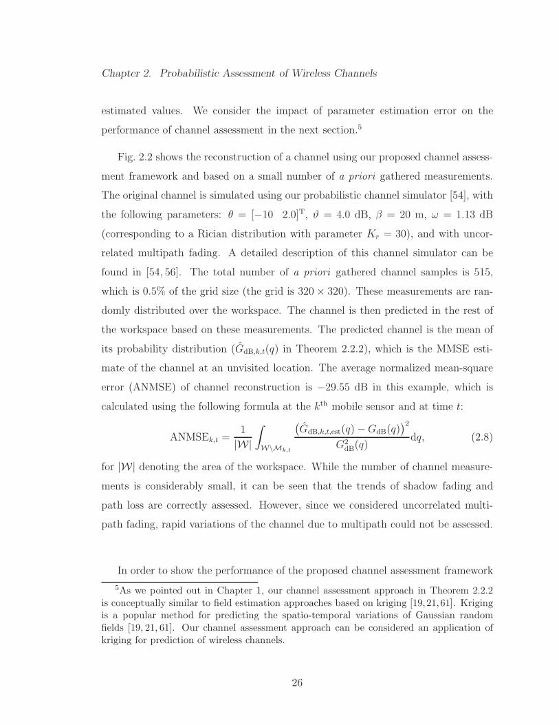
Chapter 2. Probabilistic Assessment of Wireless Channels
estimated values. We consider the impact of parameter estimation error on the
performance of channel assessment in the next section.5
Fig. 2.2 shows the reconstruction of a channel using our proposed channel assess-
ment framework and based on a small number of a priori gathered measurements.
The original channel is simulated using our probabilistic channel simulator [54], with
the following parameters: θ = [−10 2.0]T, ϑ = 4.0 dB, β = 20 m, ω = 1.13 dB
(corresponding to a Rician distribution with parameter Kr = 30), and with uncor-
related multipath fading. A detailed description of this channel simulator can be
found in [54, 56]. The total number of a priori gathered channel samples is 515,
which is 0.5% of the grid size (the grid is 320× 320). These measurements are ran-
domly distributed over the workspace. The channel is then predicted in the rest of
the workspace based on these measurements. The predicted channel is the mean of
its probability distribution (GdB,k,t(q) in Theorem 2.2.2), which is the MMSE esti-
mate of the channel at an unvisited location. The average normalized mean-square
error (ANMSE) of channel reconstruction is −29.55 dB in this example, which is
calculated using the following formula at the kth mobile sensor and at time t:
ANMSEk,t =1
|W|
∫
W\Mk,t
(GdB,k,t,est(q)−GdB(q)
)2
G2dB(q)
dq, (2.8)
for |W| denoting the area of the workspace. While the number of channel measure-
ments is considerably small, it can be seen that the trends of shadow fading and
path loss are correctly assessed. However, since we considered uncorrelated multi-
path fading, rapid variations of the channel due to multipath could not be assessed.
In order to show the performance of the proposed channel assessment framework
5As we pointed out in Chapter 1, our channel assessment approach in Theorem 2.2.2is conceptually similar to field estimation approaches based on kriging [19,21,61]. Krigingis a popular method for predicting the spatio-temporal variations of Gaussian randomfields [19, 21, 61]. Our channel assessment approach can be considered an application ofkriging for prediction of wireless channels.
26

Chapter 2. Probabilistic Assessment of Wireless Channels
Figure 2.2: A simulated channel (left) and the mean of its probability distribution(GdB,k,t(q) in Theorem 2.2.2) (right). The channel is simulated using our probabilisticchannel simulator, with the following parameters: θ = [−10 2.0]T, ϑ = 4.0 dB, β = 20 mand ω = 1.13 dB (corresponding to a Rician distribution with parameter Kr = 30). Thetotal number of a priori gathered channel samples is 515, which is 0.5% of the grid size(the grid is 320 × 320).
with real channels, Fig. 2.3 shows the reconstruction of two real channels using our
channel assessment framework. The left figure shows an outdoor channel measure-
ment across a street in downtown San Francisco (data is courtesy of Mark Smith [88])
with its reconstruction. The right figure, on the other hand, shows the reconstruction
of an indoor channel measurement along a route in our basement. For both cases,
the path loss parameters are estimated by finding the best line fit to the log of the re-
ceived measurements. After subtracting the path loss term, the channel parameters
are estimated using an approach similar to (2.4). The number of a priori channel
measurements used for parameter estimation and reconstruction is 5% of the total
samples for both channels. The channel observations are randomly distributed over
the workspace. It can be seen that the outdoor channel can be reconstructed with
a considerably better quality. This is expected as the indoor channel suffers from a
more severe multipath fading, as can be seen. Fig. 2.4 shows the reconstruction per-
formance as a function of the percentage of the measurements taken for the channels
of Fig. 2.3. It can be seen that channel estimation performance improves as more
measurements are collected.
27

Chapter 2. Probabilistic Assessment of Wireless Channels
0 2 4 6 8 10 12 14 16−95
−90
−85
−80
−75
−70
−65
−60
−55
−50
distance along the street (m)
receiv
ed
sig
nal str
en
gth
(d
Bm
)
real channel
predicted channel
6 8 10 12 14 16 18−65
−60
−55
−50
−45
−40
−35
distance from TX (m)
receiv
ed
sig
nal str
en
gth
(d
Bm
)
real channel
predicted channel
Figure 2.3: The received signal strength across a street in downtown San Francisco alongwith its reconstructed version (left) and an indoor received signal strength along a routein the basement of the ECE building at UNM and its reconstruction (right). The outdoordata is courtesy of Mark Smith. In both cases, the reconstruction is based on only 5% a
priori channel measurements.
0 0.05 0.1 0.15 0.2 0.25 0.320
25
30
35
40
45
50
55
60
% of measurements
−10lo
g10(A
NM
SE
)
0 0.05 0.1 0.15 0.2 0.25 0.321
22
23
24
25
26
27
28
% of measurements
−10lo
g10(A
NM
SE
)
Figure 2.4: Channel prediction quality for the outdoor (left) and indoor (right) channelsof Fig. 2.3, as a function of the percentage of the measurements gathered.
In the previous examples, we considered cases where the samples were randomly
distributed over the workspace. Next, we consider a more realistic case where each
mobile sensor measures the channel along its trajectory. Assume a scenario where
a number of mobile sensors are tasked with cooperatively building a map of the
spatial variations of a channel to a fixed remote station, as shown in Fig. 2.5. Each
mobile sensor measures the channel along its trajectory and shares its observations
with others for cooperative channel assessment (we assume each mobile sensor can
communicate its measurements with all the other sensors during the operation). Fig.
2.5 (left) shows the trajectories of the mobile sensors superimposed on a 2D map of
the channel power. The middle and right figures then show a snapshot of the true
28

Chapter 2. Probabilistic Assessment of Wireless Channels
channel power map and its estimate respectively, for the case where the total number
of gathered samples is 350, which is 0.34% of the grid size (the grid is 320 × 320).
The original channel is taken to be the same as in Fig. 2.2. In this case, the ANMSE
of channel reconstruction is −25.3 dB, for all the mobile sensors.
−40 −20 0 20 40−40
−30
−20
−10
0
10
20
30
40
x (m)
y (
m)
−45 dB
−31 dB
−17 dB
−3 dB
10 dB
Figure 2.5: Performance of the channel assessment framework in a cooperative channelassessment scenario – trajectories of the mobile sensors (left), a snapshot of the true channelpower map (middle) and the average of its probabilistic reconstruction using our framework(GdB,k,t(q) in Theorem 2.2.2) (right). The empty circles and the filled ones in the left figureshow the initial and final positions of the mobile sensors respectively. The original channelis the same as in Fig. 2.2. The total number of gathered samples is 350, which is 0.34% ofthe grid size.
Having an assessment of the spatial variations of the channel can be consider-
ably valuable in maintaining the connectivity of the mobile sensors in a coopera-
tive operation. In the following chapters, we show how each mobile sensor can use
our proposed channel assessment framework in order to optimize its trajectory for
communication-aware task accomplishment. More detailed discussion on our pro-
posed channel assessment framework can be found in our recent paper [89].
2.3 Sensitivity of Channel Assessment to the Es-
timation Error of the Channel Parameters
In this section, we explore the impact of error in channel parameters on the overall
channel assessment performance. Assume that estimated parameters are used for
29

Chapter 2. Probabilistic Assessment of Wireless Channels
the MMSE estimation of the channel in Theorem 2.2.2. For any q ∈ W \Mk,t, we
have
GdB(q)− GdB,k,t,est(q) = hT(q)θk,t +GSH,dB(q) +GMP,dB(q) (2.9)
− φTk,t,est(q)U
−1k,t,estHk,tθk,t − φT
k,t,est(q)U−1k,t,est
(Ξk,t + Ωk,t
),
where θk,t = θ − θk,t. Let us define the following:
∆2k,t(q) , E
(GdB(q)− GdB,k,t,est(q)
)2 ∣∣∣ θ, ϑ, β, ω, θk,t, ϑk,t, βk,t, ωk,t
. (2.10)
By conditioning on both the estimated and real parameters and using the fact that
E
(GSH,dB(q) +GMP,dB(q)
)(Ξk,t + Ωk,t
) ∣∣∣ ϑ, β, ω= φk,t(q),
E
(Ξk,t + Ωk,t
)(Ξk,t + Ωk,t
)T ∣∣∣ ϑ, β, ω= Uk,t,
E
(GSH,dB(q) +GMP,dB(q)
)2 ∣∣∣ ϑ, β, ω= ϑ2 + ω2, (2.11)
we obtain:
∆2k,t(q) = ϑ2 + ω2 − φT
k,t,est(q)U−1k,t,est
[2φk,t(q)− Uk,tU
−1k,t,estφk,t,est(q)
](2.12)
+[h(q)−HT
k,tU−1k,t,estφk,t,est(q)
]Tθk,t θ
Tk,t
[h(q)−HT
k,tU−1k,t,estφk,t,est(q)
].
Then, we have the following important question: which parameters have the most
impact on channel assessment? While we leave the proof of this to our future work,
we observed, from several channel assessments, that the channel assessment frame-
work is most sensitive to the error in path loss estimation (mainly the slope error),
which is also intuitive. Fig. 2.6 shows the impact of parameter estimation uncertainty
on the overall channel assessment quality, where the spatial average of ∆2k,t(q), i.e.,∫
W ∆2k,t
(q)dq
|W| is plotted at a sample mobile sensor and for an indoor channel with the
following parameters: θ = [−10 2.0]T, ϑ = 2.0 dB, β = 1.0 m and ω = 2.78 dB
(corresponding to a Rician distribution with parameter Kr = 5). The number of
available channel measurements is 0.1% of the total samples (102 measurements for
30

Chapter 2. Probabilistic Assessment of Wireless Channels
a 320× 320 grid), with the measurements randomly distributed over the workspace.
For each curve, only one parameter is perturbed while the rest are assumed perfect.
It can be seen that channel assessment is considerably more sensitive to path loss
parameters (specially the path loss exponent nPL). As such, it becomes important
to estimate the path loss parameters as accurately as possible. In the next section,
we show how to do so by designing a proper motion planning objective function that
is aimed at improving the estimation of path loss parameters.
−60 −40 −20 0 20 40 60
12
14
16
18
20
22
24
26
% of deviation from the exact value
sp
ati
al a
ve
rag
e o
f ∆2 k,t(q
) (d
B)
Sensitivity w.r.t. 2
Sensitivity w.r.t. β
Sensitivity w.r.t. ω2
Sensitivity w.r.t. KPL
Sensitivity w.r.t. nPL
ϑ
Figure 2.6: Spatial average of ∆2k,t(q), as a function of the % of estimation error in θk,t,
ϑ2k,t, βk,t and ωk,t.
2.4 Motion Planning for ImprovingWireless Chan-
nel Assessment in Mobile Networks
In this section, we show how each mobile sensor can use its mobility to improve
its wireless channel assessment. Consider the case that a mobile sensor is assess-
ing the spatial variations of its channel to a fixed remote station, using the channel
measurements it collects along its trajectory, as discussed in the previous section.
31

Chapter 2. Probabilistic Assessment of Wireless Channels
Since the mobile sensor measures the channel along its trajectory, its motion directly
impacts its channel assessment quality. In this section, we want to answer the fol-
lowing question: How should a mobile sensor plan its trajectory in order to improve
its channel assessment quality? We first show how a mobile sensor can plan its tra-
jectory in order to improve its estimate of the underlying channel parameters. This
is then followed by planning the motion of a mobile sensor to decrease its channel
assessment/prediction error variance.
Note that the motion planning approaches proposed in this section are greedy
approaches, i.e., they choose the locally optimal choice at each step. Generally, a
greedy approach does not guarantee finding the globally optimal solution which, in
case of our motion planning approaches, is the solution of a highly-nonlinear optimal
control problem. The reason we chose to use greedy approaches is twofold. First,
solving an optimal control problem, with a highly-nonlinear objective and over a long
time horizon, has a high computational complexity. Second, greedy approaches can
easily support adaptation. In other words, the objective function can be modified at
each step based on the newly gathered information. As shown in this section, such
adaptation is in particular useful for our motion planning approaches as the proposed
motion planning objective functions change based on the new channel measurements
that the mobile sensors gather along their trajectories (and possibly share among
each other).
2.4.1 Motion Planning for Improving the Estimation of the
Underlying Channel Parameters
Our model for the spatial variations of the channel depends on the parameters θ, ϑ,
β and ω, as discussed previously in this chapter. While the trajectory of a mobile
sensor can be optimized to improve the estimation quality of all these parameters,
32

Chapter 2. Probabilistic Assessment of Wireless Channels
we saw in Section 2.3 that channel estimation is considerably more sensitive to the
accuracy of the estimation of θ than the rest of the parameters. Therefore, in this
part we devise a motion planning strategy that aims at improving the quality of the
estimation of θ, assuming that the estimation error of the rest of the parameters
is negligible. Consider the kth mobile sensor in a multi-sensor scenario. Assume
mk,t > 0 channel measurements are available to the kth mobile sensor at time instant
t, as discussed previously in this chapter. Then, the mobile sensor needs to plan its
trajectory such that the next channel measurement it gathers optimally improves its
estimation of θ, as characterized by the next theorem. In this theorem, we consider
the more challenging case of maximum likelihood (ML) estimation of the path loss
parameters. The result can be easily modified for the simpler case of LS estimation.
Theorem 2.4.1. Assume negligible error in the estimation of ϑ, β and ω. Let CML,k,t
denote the error covariance of the ML estimation of the path loss parameters at the
kth mobile sensor and at time t, conditioned on shadowing and multipath parameters.
Assume that the kth mobile sensor gathers one more channel power measurement
along its trajectory at time t+ 1. Then we have the following recursion for CML,k,t:
C−1ML,k,t+1 = C−1
ML,k,t (2.13)
+
[hT(ξk,t+1)− φT
k,t(ξk,t+1)U−1k,tHk,t
]T[hT(ξk,t+1)− φT
k,t(ξk,t+1)U−1k,tHk,t
]
σ2k,t(ξk,t+1)
,
where ξk,t+1 is the position of the jth mobile sensor at time k + 1.
Proof. Based on the probabilistic modeling of the previous section, the ML estima-
tion of θ and its corresponding estimation error covariance, using the channel power
measurements up to time t+ 1 and conditioned on ϑ, β and ω, are given as follows:
θML,k,t+1 =(HT
k,t+1U−1k,t+1Hk,t+1
)−1HT
k,t+1U−1k,t+1Yk,t+1,
CML,k,t+1 =(HT
k,t+1U−1k,t+1Hk,t+1
)−1, (2.14)
33

Chapter 2. Probabilistic Assessment of Wireless Channels
where Uk,t+1 =
ϑ2 + ω2 φTk,t
(ξk,t+1
)
φk,t
(ξk,t+1
)Uk,t
and Hk,t+1 =[h(ξk,t+1) HT
k,t
]T. Note that
we take ξk,t+1 6∈ Mk,t. By using matrix inversion lemma [90] for U−1k,t+1 we have:
U−1k,t+1 =
1σ2k,t
(ξk,t+1)
φTk,t
(ξk,t+1)U−1k,t
σ2k,t
(ξk,t+1)
U−1k,t
φk,t(ξk,t+1)
σ2k,t
(ξk,t+1)U−1k,t +
U−1k,t
φk,t(ξk,t+1)φTk,t
(ξk,t+1)U−1k,t
σ2k,t
(ξk,t+1)
(2.15)
where σ2k,t
(ξk,t+1
)= ϑ2 + ω2 − φT
k,t
(ξk,t+1
)U−1k,t φk,t
(ξk,t+1
). By multiplying U−1
k,t+1
from left by HTk,t+1 and from right by Hk,t+1, and by using the fact that C−1
ML,k,t =
HTk,tU
−1k,tHk,t, (2.13) is obtained.
Our proposed approach to minimize the estimation error covariance of θ in the
next step is to have the kth mobile sensor maximize the second term on the right
hand side of (2.13) at any time t. Consider the following discrete dynamical model
for the kth mobile sensor: ξk,t+1 = Υk(ξk,t, uk,t), where uk,t ∈ Uk is the control input
at time t, Uk is the set of admissible control inputs and Υk(., .) is a known function.
We then have the following next-step motion optimization problem, considering the
trace of the right hand side of (2.13):
u∗k,t = argmaxuk,t
JPL,k,t(ξk,t+1) ,
∥∥hT(ξk,t+1)− φTk,t,est(ξk,t+1)U
−1k,t,estHk,t
∥∥2
σ2k,t,est(ξk,t+1)
s.t. 1) ξk,t+1 = Υk
(ξk,t, uk,t
), 2) uk,t ∈ Uk, 3) ξk,t+1 ∈ W \ Ok,t, (2.16)
where φk,t,est(q), Uk,t,est and σ2k,t,est(q) are the estimates of φk,t(q), Uk,t and σ
2k,t(q), with
the shadowing and multipath parameters replaced by their estimated values. Also,
Ok,t denotes the set of forbidden areas for obstacle/collision avoidance, estimated by
the kth mobile sensor at time t.
Note that we do not consider coordination among the mobile sensors when plan-
ning their motion in (2.16). However, the sensors can share their gathered channel
measurements and their positions as they move. The shared information can be used
34
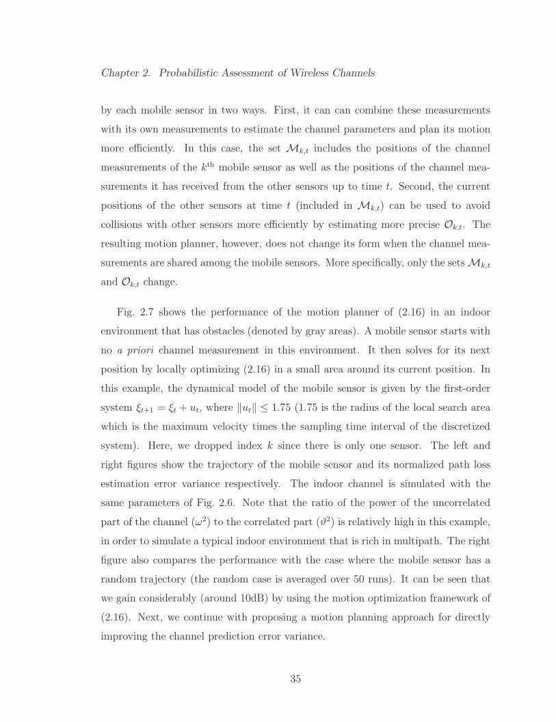
Chapter 2. Probabilistic Assessment of Wireless Channels
by each mobile sensor in two ways. First, it can can combine these measurements
with its own measurements to estimate the channel parameters and plan its motion
more efficiently. In this case, the set Mk,t includes the positions of the channel
measurements of the kth mobile sensor as well as the positions of the channel mea-
surements it has received from the other sensors up to time t. Second, the current
positions of the other sensors at time t (included in Mk,t) can be used to avoid
collisions with other sensors more efficiently by estimating more precise Ok,t. The
resulting motion planner, however, does not change its form when the channel mea-
surements are shared among the mobile sensors. More specifically, only the sets Mk,t
and Ok,t change.
Fig. 2.7 shows the performance of the motion planner of (2.16) in an indoor
environment that has obstacles (denoted by gray areas). A mobile sensor starts with
no a priori channel measurement in this environment. It then solves for its next
position by locally optimizing (2.16) in a small area around its current position. In
this example, the dynamical model of the mobile sensor is given by the first-order
system ξt+1 = ξt + ut, where ‖ut‖ ≤ 1.75 (1.75 is the radius of the local search area
which is the maximum velocity times the sampling time interval of the discretized
system). Here, we dropped index k since there is only one sensor. The left and
right figures show the trajectory of the mobile sensor and its normalized path loss
estimation error variance respectively. The indoor channel is simulated with the
same parameters of Fig. 2.6. Note that the ratio of the power of the uncorrelated
part of the channel (ω2) to the correlated part (ϑ2) is relatively high in this example,
in order to simulate a typical indoor environment that is rich in multipath. The right
figure also compares the performance with the case where the mobile sensor has a
random trajectory (the random case is averaged over 50 runs). It can be seen that
we gain considerably (around 10dB) by using the motion optimization framework of
(2.16). Next, we continue with proposing a motion planning approach for directly
improving the channel prediction error variance.
35

Chapter 2. Probabilistic Assessment of Wireless Channels
−40 −20 0 20 40−40
−20
0
20
40
x (m)
y (
m)
base station
10 20 30 40 50
−15
−10
−5
0
5
10
15
20
25
time step (t)
no
rmalized
err
or
vari
an
ce (
dB
)
KPL
(comm. aware traj.)
nPL
(comm. aware traj.)
KPL
(random traj.)
nPL
(random traj.)
Figure 2.7: Trajectory of a mobile mobile sensor in communication-aware motion planningfor improving path loss parameter estimation in an indoor environment (left) and thecorresponding normalized estimation error variance (right). The empty circle and thefilled one in the left figure denote the initial and final positions of the mobile sensor.
2.4.2 Motion Planning for Reducing the Channel Assess-
ment Uncertainty
Once the parameters of the underlying model are estimated, the mobile sensor can
plan its trajectory in order to reduce its channel assessment/prediction uncertainty.
As characterized in Theorem 2.2.2, the error variance of the channel assessment at
the kth mobile sensor at time t is as follows: σ2k,t(q) = ϑ2 + ω2 − φT
k,t(q)U−1k,t φk,t(q),
for any q ∈ W \ Mk,t and assuming negligible error in the underlying parameters.
Consider the case where a number of channel measurements are available to the kth
mobile sensor at time t. Then, the mobile sensor can plan its motion to go towards
the location with the highest channel assessment uncertainty, i.e., the largest σ2k,t(q),
based on the available measurements.6 Define the following objective function:
JCH,k,t(q) , max0, σ2
k,t,est(q)− σ2TH
ψ(‖q − ξk,t‖
), (2.17)
where σ2k,t,est(q) is the estimate of σ2
k,t(q), with the exact parameters replaced by
the estimated ones, σ2TH is a fixed threshold and ψ(.) is a non-increasing function
6Alternatively, the mobile sensor can plan its motion in order to minimize the spatialaverage of the channel assessment uncertainty over the entire workspace of interest [7].
36

Chapter 2. Probabilistic Assessment of Wireless Channels
of its argument. By thresholding σ2k,t,est(q), we remove the positions with negligible
channel assessment uncertainty. Then, ψ(‖q − ξk,t‖
)weighs the remaining space
based on closeness to the current position, favoring less movement. Let q∗k,t denote
the maximizing argument of the JCH,k,t(q) over the workspace:
q∗k,t , argmaxq∈W\Mk,t∪Ok,t
JCH,k,t(q) (2.18)
Here, q∗k,t is an obstacle/collision free position with high channel assessment uncer-
tainty, that is also close to the current position of the mobile sensor. If motion cost
is not an issue, ψ can be chosen one. In our results, we take ψ(d) = e−ζd, for ζ ≥ 0.
The motion of the kth mobile sensor at time t (the corresponding control input) is
then the solution of the following optimization problem:
u∗k,t = argminuk,t
∥∥ξk,t+1 − q∗k,t∥∥ for q∗k,t = argmax
q∈W\Mk,t∪Ok,t
JCH,k,t(q)
s.t. 1) ξk,t+1 = Υk
(ξk,t, uk,t
), 2) uk,t ∈ Uk, 3) ξk,t+1 ∈ W \ Ok,t. (2.19)
As can be seen from (2.19), the motion of the kth mobile sensor is planned based
on its current estimate of the channel assessment error variance. Similar to motion
planning for improving the estimation of the channel parameters, sharing the channel
measurements and the positions of the mobile sensors can be useful in two ways.
First, each mobile can combine these measurements with its own ones to assess
the channel and plan its motion more efficiently. The extra channel measurements
prevent the mobile sensor from visiting previously-explored areas by other sensors,
which results in a much faster reduction in the overall channel assessment error
variance. Second, the current positions of the other sensors at time t can be used to
avoid collisions with other sensors by estimating a more precise Ok,t. However, the
form of the motion planner does not change by sharing the channel measurements
and positions among the mobile sensors.
Fig. 2.8 shows the performance of this motion planning approach for a single
mobile sensor in an outdoor environment with obstacles (denoted by gray areas),
37

Chapter 2. Probabilistic Assessment of Wireless Channels
where we assumed negligible error in the estimation of the modeling parameters. The
dynamical model of the mobile sensor is given by ξt+1 = ξt + ut, where ‖ut‖ ≤ 5.5.
The outdoor channel is simulated with the following parameters: θ = [−10 2],
ϑ = 4 dB, β = 10.0 m and ω = 2 dB (for a Rician distribution with Kr = 10).
Furthermore, σ2TH = 4 and ζ = 0.02. The mobile sensor starts with 0.016% a priori
channel measurements, randomly chosen in the space (0.016% of the total number
of workspace samples, i.e., 16 measurements for a 320×320 grid). Fig. 2.8 (left) and
(right) show the trajectory of the mobile sensor and the time evolution of ANMSE
of the channel assessment respectively. For the sake of comparison, the right figure
also compares the performance with the case where the mobile sensor has a random
trajectory (the random case is averaged over 50 runs). It can be seen that channel
assessment uncertainty reduces considerably as the mobile sensor intelligently plans
its motion. In terms of computational complexity, solving the optimization problem
of (2.19) at each step, for a 320×320 grid, took 2.4 seconds (on average) on a desktop
with the Intel Core 2 vPro processor and 2 GB of RAM.
−40 −20 0 20 40−40
−30
−20
−10
0
10
20
30
40
x (m)
y (
m)
50 100 150
−24
−23
−22
−21
−20
−19
−18
−17
time step (t)
AN
MS
E o
f ch
an
nel assessm
en
t (d
B)
comm. aware traj.
random traj.
Figure 2.8: Trajectory of a mobile mobile sensor in communication-aware motion planningfor reducing channel assessment uncertainty in an outdoor environment (left) and thecorresponding ANMSE (right). The empty circle and the filled one in the left figure denotethe initial and final positions of the mobile sensor.
38

Chapter 2. Probabilistic Assessment of Wireless Channels
Finally, Fig. 2.9 shows the snapshots of the spatial variations of the channel
assessment error variance over the workspace and for four different time instants. It
can be seen that channel prediction improves considerably with time, as the mobile
sensor intelligently optimizes its motion accordingly.
Figure 2.9: Snapshots of the channel assessment error variance over the workspace (topleft for t = 0, top right for t = 50, bottom left for t = 100 and bottom right for t = 200)
2.5 Summary
In this chapter, we first showed how a mobile sensor can assess (predict) the spatial
variations of a wireless channel based on a small number of channel measurements.
We then showed how to plan motion of the mobile sensor to improve its channel
assessment performance. Our proposed probabilistic channel assessment framework
39

Chapter 2. Probabilistic Assessment of Wireless Channels
is built on the well-established multi-scale model of wireless channels and enables
a mobile sensor to efficiently predict the channel along its trajectory. To improve
its channel assessment performance, the mobile sensor can then use one of the two
proposed motion planning strategies of this chapter to either improve its estimate of
the underlying model parameters or decrease the channel predication error variance.
In the following chapters, we show how the proposed channel assessment frame-
work of this chapter can be integrated with motion planning in order to improve the
connectivity of the mobile sensors while accomplishing their networked task.
40

Chapter 3
Communication-Aware Target
Tracking Using Mobile Networks
In this chapter, we study the problem of networked target tracking in realistic com-
munication environments. We consider the scenario where a fixed remote station
utilizes a mobile sensor (or a number of them) for keeping track of the position of a
moving target. The communication links between the mobile sensor and the remote
station are realistic wireless link that experiences path loss, shadowing and multipath
fading. We first characterize the estimation error covariance of target position at the
remote station when 1) a realistic packet-dropping receiver is used at the remote
station which drops the received packets based on the instantaneous received SNR
and 2) a Kalman filter is used to fuse the received noisy sensory data at the remote
station. This error covariance depends on both the sensing quality of the mobile
sensors along their trajectories and the quality of their channels to the remote sta-
tion. We then propose novel decentralized communication-aware motion planning
approaches that integrate sensing and communication objectives to minimize the es-
timation error covariance of target position at the remote station. A schematic of
the networked target tracking scenario considered in this chapter is shown in Fig.
41

Chapter 3. Communication-Aware Target Tracking Using Mobile Networks
3.1.
mobile sensorremote station
moving
target
wireless link
sensing
trajectory of the node
sensor trajectory
Figure 3.1: A schematic of the networked target tracking operation considered in thischapter.
Note that in order for the mobile sensors to assess the proposed objective functions
(or constrains) at positions that have not yet been visited by any mobile sensor, the
channel assessment framework of Chapter 2 is used. Also note that we do not consider
any coordination among the nodes for the purpose of target tracking. In other words,
each mobile sensor plans its motion individually. However, as explained in Section
2.4, the mobile sensors can still share their channel measurements and their positions
in order to assess the channel and avoid collisions more efficiently. Finally, similar
to the motion planning approaches of Section 2.4, the proposed motion planning
approaches of this chapter are greedy to avoid high computational complexity and
better facilitate adaptation.
The rest of the chapter is organized as follows. In Section 3.1, we describe our
system model and present the Kalman filtering equations for target tracking over
realistic communication links. In Section 3.2, we propose our communication-aware
motion planning approaches and mathematically analyze their performance. We
present our simulation and experimental results in Section 3.3, followed by a summary
of the chapter in Section 3.4.
42

Chapter 3. Communication-Aware Target Tracking Using Mobile Networks
3.1 Problem Formulation
Consider the case where a fixed remote station utilizes n mobile sensors for keeping
track of a position of a moving target in a workspace W ⊂ R2, which is assumed
to be closed and convex [91]. The overall goal is for the station to constantly have
a good assessment of the target position. The communication links between the
mobile sensors and the base station experience path loss, shadowing and multipath
fading. We consider a realistic packet-dropping receiver [6,92] at the remote station,
i.e., the remote station drops all the packets with the received SNR (or equivalently
the received channel power) below a predefined threshold. Note that in practice,
the receiver drops the packets based on the quality of decoding. However, in [93],
the authors show that this is equivalent to having a received SNR threshold. Let
SNRTH denote this SNR threshold. Then, the received packet from the kth mobile
sensor is dropped at time t if SNR(ξk,t) < SNRTH, and is kept otherwise. Here,
SNR(q) is the received SNR at the remote station when mobile sensor is at position
q ∈ W. Without loss of generality, assume that all the mobile sensors use a fixed
transmit power PTX. From Chapter 2, for any q ∈ W we have SNR(q) = PTXG(q)BN0
,
where B is the transmission bandwidth and N0
2is the power spectral density (PSD)
of the thermal noise at the receiver of the remote station. Then, SNR(ξk,t) < SNRTH
results in
GdB(ξk,t) < 10 log10
(SNRTHBN0
PTX
), GdB,TH, (3.1)
where GdB,TH is the equivalent packet dropping threshold for channel power in dB
(see Chapter 2 for more details).
Let us define xt ,[pTt pTt
]T, with pt ∈ R
2 and pt ∈ R2 denoting the position
and velocity of the target respectively at time t. Also, let yk,t ∈ R2 represent the
measurement of the kth mobile sensor of xt at time t. We consider the following
43

Chapter 3. Communication-Aware Target Tracking Using Mobile Networks
dynamical and observation models [94]:
xt+1 =
I2 tsI2
0 I2
︸ ︷︷ ︸A
xt +
12t2sI2
tsI2
︸ ︷︷ ︸B
wt, yk,t =[I2 0
]
︸ ︷︷ ︸C
xt + vk,t, (3.2)
where ts is the sampling period used to discretize the dynamics of the target, wt ∈ R2
and vk,t ∈ R2 are zero-mean Gaussian noises, with W = E
wkw
Tk
and Vk,t =
Evk,tv
Tk,t
representing their covariance matrices respectively, and I2 is the 2 × 2
identity matrix. Note that Vk,t depends on the position of the kth mobile sensor as
well as the position of the target [7, 94]: Vk,t = Φ(ξk,t, pt
), where Φ(., .) is assumed
known.
The remote station constantly estimates the position of the target, based on
its received observations and by using a Kalman filter. We assume that when the
received packet from a mobile sensor is kept at the remote station, it is error-free.
This is the case when SNRTH is large enough. We therefore consider the following
assumption throughout the rest of this chapter:
Assumption 3.1.1. The packet-dropping threshold SNRTH is large enough, or equiv-
alently the performance of the decoding algorithm at the remote station is good
enough, such that the packets that are kept at the remote station can be considered
error-free.
Note that Assumption 3.1.1 is a valid for a large class of existing receivers used in
robotics and sensor network applications. Now, let xt1|t2 represent the estimate of xt1
at the remote station, using all the received observations up to and including time t2.
Also, let Πt1|t2 denote the corresponding estimation error covariance at the remote
station, given GdB(ξk,0), · · · , GdB(ξk,t2), for t2 ≤ t1 and k = 1, · · · , n. Assuming
i.i.d. observations and based on Assumption 3.1.1, the Kalman filter equations for
44

Chapter 3. Communication-Aware Target Tracking Using Mobile Networks
estimating xt is given as follows [95]:
xt+1|t = A xt|t,
Πt+1|t = AΠt|tAT +BWBT,
xt+1|t+1 = xt+1|t +Πt+1|tCT(CΠt+1|tC
T+ V t+1
)−1(yt+1 − Cxt+1|t
),
Πt+1|t+1 = Πt+1|t −Πt+1|tCT(CΠt+1|tC
T+ V t+1
)−1CΠt+1|t, (3.3)
where C ,[CT · · ·CT
]Tis the matrix of the stacked observation matrices of all the
mobile sensors, yt+1 ,[yT1,t+1 · · · yTn,t+1
]Tis the vector of stacked observations of the
mobile sensors and V t+1 = diag(
V1,t+1
λ1,t+1, · · · , Vn,t+1
λn,t+1
). Here, the binary variable λk,t
captures the effect the packet-dropping receiver of the remote station and is defined
as follows:
λk,t ,
1, GdB(ξk,t) ≥ GdB,TH,
0, else(3.4)
Using the definition of V t+1, one can see that whenever the received packet from the
kth mobile sensor is dropped at time t+ 1, its corresponding diagonal block in V t+1
becomes infinite, which implies that the observation of the kth mobile sensor does not
contribute to the estimation process at that time. This becomes more clear by using
the information form of the Kalman filters [95]. Let us define the Fisher information
matrix as Γt1|t2 , Π−1t1|t2 . Then, by using the information form of Kalman filter,
which is a direct result of applying the matrix inversion lemma, a recursion for Γt|t
is given as follows:
Γt+1|t =(AΓ−1
t|t AT +BWBT
)−1
,
Γt+1|t+1 = Γt+1|t +n∑
k=1
λk,t+1CTV −1
k,t+1C︸ ︷︷ ︸,Λk,t+1
, (3.5)
where Λk,t+1 is the information contribution of the kth mobile sensor at time t + 1.
As can be seen, the Fisher information at the remote station will be dictated by
45

Chapter 3. Communication-Aware Target Tracking Using Mobile Networks
the dynamics of the target as well as the summation of the information contribution
terms, i.e.,∑n
k=1 Λk,t+1. Next we show how to plan the motion of the mobile sensors
at each step to maximize the average Fisher information at the remote station.
3.2 Communication-Aware Target Tracking Using
Probabilistic Assessment of Wireless Chan-
nels
The information innovation term Λk,t+1 in (3.5) depends on both the sensing quality
of the kth mobile sensor as well as its communication link quality to the remote
station. Since our assessment of the link qualities is probabilistic, Λk,t+1 also becomes
stochastic due to its dependency on the link qualities. By averaging over channel
distributions, we have
EΓt+1|t+1
= E
Γt+1|t+
n∑
k=1
EΛk,t+1
, (3.6)
where
EΛk,t+1
= E
λk,t+1
CTV −1
k,t+1C
= P
GdB
(ξk,t+1
)≥ GdB,TH
CTV −1
k,t+1C. (3.7)
In this equation, PGdB
(ξk,t+1
)≥ GdB,TH
is the probability that the received packet
from the kth mobile sensor is kept at the remote station at time t+1. At any time t,
the next step average Fisher information at the remote station is maximized if the kth
mobile sensor maximizes its assessment of EΛk,t+1
. The kth mobile mobile sensor
can assess PGdB
(ξk,t+1
)≥ ΥdB,TH
by using the channel assessment framework of
Chapter 2 as follows:
P
GdB
(ξk,t+1
)≥ GdB,TH
= Q
(GdB,TH − GdB,k,t,est(ξk,t+1)
σk,t,est(ξk,t+1)
), (3.8)
46

Chapter 3. Communication-Aware Target Tracking Using Mobile Networks
where Q(a) = 1√2π
∫∞ae−s2/2ds is the Q-function (the tail probability of normal dis-
tribution). Also, GdB,k,t,est(q) and σk,t,est(q) are the estimates of GdB,k,t(q) and σk,t(q)
respectively (see Theorem 2.2.2), with the exact parameters replaced by the esti-
mated ones.
Our first proposed approach is to plan the motion of the mobile sensors at time
t such that the trace of EΓt+1|t+1
is maximized. This is equivalent to maximizing
the trace of∑n
k=1EΛk,t+1
, which results in the following optimization problem for
finding the control input of the kth mobile sensor at time t:
u∗k,t = argmaxuk,t
JTRCK1,k,t(ξk,t+1) , Q
(GdB,TH − GdB,k,t,est
(ξk,t+1
)
σk,t,est(ξk,t+1
))
︸ ︷︷ ︸Comm. obj.
× trΦ−1
(ξk,t+1, pk,t+1|t
)
︸ ︷︷ ︸Sensing obj.
s.t. 1) ξk,t+1 = Υk
(ξk,t, uk,t
), 2) uk,t ∈ Uk, 3) ξk,t+1 ∈ W \ Ok,t. (3.9)
Here, ξk,t+1 = Υk(ξk,t, uk,t), for known Υk(., .), denotes the dynamical model of the
kth mobile sensor, uk,t ∈ Uk is the control input of the kth mobile sensor at time t
and Uk is the set of its admissible control inputs. Also, pk,t+1|t is the prediction of the
kth mobile sensor of the target position at time t+ 1, which it can assess by using a
local Kalman filter. The set Ok,t includes the forbidden positions that are excluded
to avoid obstacles/collisions. The objective function of (3.9) shows how channel
learning is integrated with sensing objectives in order to ensure communication-
aware operation. A mobile sensor can start with a priori channel measurements in
the environment for channel assessment. It then improves its channel assessment as
it gathers more measurements along its trajectory, while simultaneously tracking the
target using (3.9).
As can be seen, by using the trace of EΓt+1|t+1
, the overall objective of the next
step information maximization at the remote station decouples into maximizing n
47

Chapter 3. Communication-Aware Target Tracking Using Mobile Networks
localized objective functions at the individual mobile sensors. In case other metrics
are used (e.g. det(.) or ‖.‖), the objective function may not be decentralizable,
requiring coordination and sharing the position of the mobile sensors among them.
Note that sharing the positions (and the channel measurements) is useful even when
the decentralized motion planning approach of (3.9) is used. As explained in Section
2.4, each mobile sensor can use the channel measurements and the positions of the
other sensors up to time t to better assess the channel. This makes the Q-function
term in the objective function of (3.9) a more precise estimate of the probability of
connectivity. Additionally, by using the current positions of other mobile sensors,
the set Ok,t will be a more reliable set for collision avoidance.
Using the motion planning approach of (3.9), the mobile sensors improve their
probability of connectivity while tracking the target. Next, we mathematically show
that in case the channel is assessed perfectly, the motion planning approach of (3.9)
maintain the connectivity of the mobile sensors. By perfect channel assessment we
mean the following:
Definition 3.2.1. Perfect channel assessment refers to the case where the channel
is predicted perfectly. For instance, if the multipath fading power is negligible, the
channel parameters are known perfectly and the number of channel measurements
are large enough such that σk,t(q) → 0, for all k, q ∈ W and t ≥ 0, then the channel
is predicted perfectly.
We then have the following theorem in case of perfect channel assessment:
Theorem 3.2.1. Assume that the channel is assessed perfectly. Define the time-
invariant set Wc ,q ∈ W
∣∣GdB,k,t,est(q) ≥ GdB,TH
as the connected region, which
is assumed to be closed. Then, if ξk,0 ∈ Wc for all k, the motion planning approach
of (3.9) maintain the connectivity of the mobile sensors, i.e., it ensures ξk,t ∈ Wc for
all k and t > 0.
48

Chapter 3. Communication-Aware Target Tracking Using Mobile Networks
Proof. In case the channel is assessed perfectly, the Q-function in (3.9) acts as a hard
limiter and becomes one if ξk,t+1 ∈ Wc, and zero otherwise. Therefore, if ξk,t ∈ Wc,
the solution of (3.9) is a point ξk,t+1 ∈ Wc, which has this property that the kth
mobile sensor can be navigated to this point at time t + 1, without any collision or
violating the constraints imposed by its dynamics. This proves that if ξk,0 ∈ Wc,
then ξk,t ∈ Wc for all t > 0. Note that we assumed that 1) Uk ∋ 0 and 2) when
uk,t = 0 then Υk
(ξk,t, uk,t
)= ξk,t.
From Theorem 3.2.1, one can observe that in case of perfect channel assessment,
the optimization problem of (3.9) is equivalent to the following:
u∗k,t = argmaxuk,t
trΦ−1
(ξk,t+1, pk,t+1|t
)(3.10)
s.t. 1) ξk,t+1 = Υk
(ξk,t, uk,t
), 2) uk,t ∈ Uk, 3) ξk,t+1 ∈ Wc \ Ok,t.
In other words, in order to ensure communication-awareness in this case, it is suffi-
cient to limit the motion of the mobile sensors to the connected region Wc and only
consider the sensing objective. This motivates our second motion planning approach
for communication-aware target tracking. In this approach, we limit the motion of
the mobile sensors to the areas with good probability of connectivity. More specifi-
cally, we plan the motion of the kth mobile sensor to guarantee that, if the channel
is not assessed perfectly, PGdB
(ξk,t+1
)≥ GdB,TH
≥ 1 − ε, for all k and an arbi-
trary small 0 < ε < 1, while maximizing the trace of CTV −1k,t+1C. This results in the
following motion optimization problem to find the control input of the kth mobile
sensor at time t:
u∗k,t = argmaxuk,t
JTRCK2,k,t(ξk,t+1) , trΦ−1
(ξk,t+1, pk,t+1|t
)
︸ ︷︷ ︸Sensing obj.
s.t. 1) Q
(GdB,TH − GdB,k,t,est
(ξk,t+1
)
σk,t,est(ξk,t+1
))
≥ 1− ε
︸ ︷︷ ︸Comm. constraint
,
2) ξk,t+1 = Υk
(ξk,t, uk,t
), 3) uk,t ∈ Uk, 4) ξk,t+1 ∈ W \ Ok,t. (3.11)
49

Chapter 3. Communication-Aware Target Tracking Using Mobile Networks
It can be seen that in case of perfect channel assessment, (3.9) and (3.11) are equiv-
alent and are reduced to (3.10).
We next continue with analyzing the convergence properties of the proposed
motion planning approaches. We have the following theorem:
Theorem 3.2.2. Consider the case where the channel is assessed perfectly. Assume
that the collision among the mobile sensors is negligible. Let O ⊂ W denote the
open set of obstacles and define Wc,f , Wc \ O to be the obstacle-free connected
region (obstacle-free region with GdB,k,t,est(q) ≥ GdB,TH). Assume that Wc,f is a
closed set and ξk,0 ∈ Wc,f for all k. Also, assume that the target is static and located
at p0 ∈ W. Define the function ϕ : Wc,f → R+ such that ϕ(q) = trΦ−1(q, p0)
.
Also, for any q ∈ R2, define the reachable set of the kth sensor as Rk(q) ,
q′ ∈
R2∣∣q′ = Υk(q, u), u ∈ Uk
, which is assumed to be a closed and connected set (not to
be confused with the connected region Wc). Assume there exists an r > 0 such that
Rk(q) ⊇ B(q, r), where B(q, r) is the disk with radius r centered at q ∈ Wc,f . Then,
each mobile sensor converges to a local maximum of ϕ over Wc,f (which could be on
the boundary of Wc,f) using (3.9) or (3.11).
Proof. As proved by Theorem 3.2.1, in case the collision among the mobile sensors
is negligible and they start in Wc,f , they will remain in Wc,f using (3.9) or (3.11).
At each time t, the next position of the kth sensor is found as follows: ξk,t+1 =
argmaxq∈Rk,f (q)trΦ−1
(q, pk,t+1|t
), where Rk,f(q) , Rk(q)∩Wc,f . Since the target
is stationary, each mobile sensor can asymptotically estimate the position of the
target using its local Kalman filter, i.e., pk,t+1|t → p0. Also, since both Wc,f and
Rk(q) are closed and Rk(q) ⊇ B(q, r) for some r > 0, then there always exists a
ρ(q) > 0 such that Rk,f(q) ⊇ B(q, ρ(q)
)for each q ∈ Wc,f \ ∂Wc,f , where ∂Wc,f
denotes the boundary of Wc,f (note that Wc,f is a closed set). This ensures that the
dynamics of the mobile sensor is such that it can move in any direction unless it hits
the boundary of Wc,f . Thus, it will eventually converge to a local maximum of ϕ(q)
50

Chapter 3. Communication-Aware Target Tracking Using Mobile Networks
over Wc,f , which could be in Wc,f \ ∂Wc,f or on the boundary ∂Wc,f .
Using Theorem 3.2.2, one can immediately conclude that if the smooth ϕ(q) has
a unique maximum and attains its global maximum inside Wc,f , then the mobile
sensors will eventually converge to this global maximum of ϕ(q), provided that the
conditions of Theorem 3.2.2 hold. Note that the condition Rk(q) ⊇ B(q, r) in Theo-
rem 3.2.2 guarantees that the mobile sensor can move in every direction at any point
along its trajectory unless it is on the boundary of the workspace. In case the dy-
namical model of the mobile sensor limits its direction of the movement, convergence
may not happen.
3.2.1 Discussion on Local Extrema Avoidance
Local extrema avoidance is an important issue in motion planning [28, 29]. Re-
searchers have proposed several methods to design motion planners that can avoid
local extrema. The approaches based on the well-known Navigation Functions, for
instance, are good examples [29, 96].
In our proposed motion planning framework of this chapter, we solve the resulting
optimization problems through a local greedy search (dictated by constraints 1 and
2 of (3.9) or constraints 2 and 3 of (3.11)). Thus, our framework naturally suffers
from local extrema. Although, we emphasize that by enlarging the search space (if
permitted computationally) and/or separating the optimization of the best next step
from path planning, local extrema could be avoided. For instance, by enlarging the
reachable set Rk(q) (defined in Theorem 3.2.2), we can lower the chance of getting
trapped in a local extremum. In the extreme case where the workspace is obstacle-
free, W ⊆ Rk(q), the channel is assessed perfectly as t → ∞, and the target is
stationary, asymptotically the mobile sensors converge to the global maxima of ϕ(q).
There is, however, a constraint on the size of the reachable set of the mobile sensors.
51

Chapter 3. Communication-Aware Target Tracking Using Mobile Networks
Generally, the size of Rk(q) is dictated by the sampling period ts and the dynamics
of the kth sensor. For a very small ts the size of Rk(q) is small unless the mobile
sensors can move very fast. So, the reachable sets should be chosen as larger as
possible within the constraints imposed by the dynamics of the mobile sensors.
Also, note that the time variation of the objective function/constraints, due to
the movement of the target and/or the new channel measurements gathered along
the trajectory, is also a mechanism that may prevent the mobile sensors from being
trapped in local extrema. This mechanism is specially useful in practical applications
where the channel assessment is not perfect.
3.3 Simulation and Experimental Results
In this section, we present the results of applying the proposed communication-aware
framework to two examples with simulated and real channels. For the sake of brevity,
we use the motion optimization approach of (3.9) in these example. Similar behaviors
can be observed if (3.11) is instead used.
Fig. 3.2 shows a target tracking scenario in an outdoor environment that con-
tains obstacles (gray areas), using three mobile sensors. We use mobile agents with
the following dynamics: ξk,t+1 = ξk,t + uk,t, for ‖uk,t‖ ≤ 2.0. We furthermore
assume the position-dependent model of [7] for the observation noise covariance:
trΦ−1(ξk,t, pt)
= 1
g(‖ξk,t−pt‖) , where g(r) = (r − rs)2 + ν, > 0 and ν > 0 are
scaling constants, and rs is the sweet spot radius at which the sensing quality is the
best. For this example we use = 0.008, ν = 0.08 and rs = 1.0 m. The outdoor
channel is simulated using the following parameters: θ = [−10 2.0]T, ϑ = 4.0 dB,
β = 20 m and ω = 1.13 dB (corresponding to a Rician distribution with Kr = 30).
Furthermore, ts = 0.5 s, W = 0.001I2 and GdB,TH = −40 dB. In order to com-
pare the performance of our communication-aware framework with more traditional
52

Chapter 3. Communication-Aware Target Tracking Using Mobile Networks
approaches, the figure shows four different cases: 1) comm-aware, 2) comm-aware
(PL-only), 3) informed disk model and 4) comm-unaware. Comm-aware case is the
full communication-aware framework of (3.9). On the other hand, comm-aware (PL-
only) is a simplified yet probabilistic version of our framework where the correlation
of the shadowing part is not utilized. In this case, the average of the channel is esti-
mated by considering only the path loss parameters in (3.9) (GdB,k,t,est(q) = hT(q) θk,t
in Theorem 2.2.2) and the variance is calculated accordingly. As we shall see from
our results, this approach is more suitable for the cases where the environment is
multipath dominant (experiencing a small ratio of the correlated channel component
to the uncorrelated part). Informed disk model is the case where each mobile sensor
models the link with a disk model (which is common in the robotics literature). How-
ever, it is a more informed approach, in which our channel assessment framework is
utilized to assess the path loss decay rate. Then a disk is specified based on GdB,TH.
Finally, the comm-unaware case is the case where each mobile sensor only considers
its sensing objectives. Fig. 3.2 (left) shows the trajectories of the mobile sensors
for comm-aware (solid magenta lines) and comm-unaware (dashed red lines) cases,
superimposed on the connectivity map of the received channel power to the remote
station, with the white (black) regions denoting the connected (disconnected) areas.
For better visualization, we did not include the trajectories of the other two cases.
The performance of all the four cases is then compared in Fig. 3.2 (right), where the
trace of the average normalized error covariance of target position estimation at the
remote station (averaged over 30 runs) is plotted as a function of time. It can be
seen that the communication-aware case performs considerably better than the other
approaches as it maintains the connectivity of the mobile sensors to the remote sta-
tion with high probability. This is then followed by the performance of the PL-only
case, informed disk model and the unaware case, as expected. Note that in all the
cases, each mobile sensor solves for its corresponding next-step motion optimization
problem locally, in a small area around it. Furthermore, in all the cases, the mobile
53
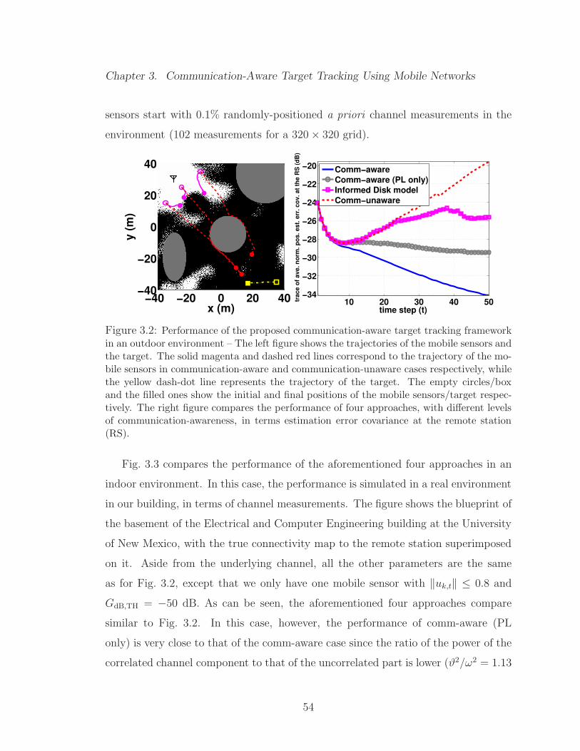
Chapter 3. Communication-Aware Target Tracking Using Mobile Networks
sensors start with 0.1% randomly-positioned a priori channel measurements in the
environment (102 measurements for a 320× 320 grid).
−40 −20 0 20 40−40
−20
0
20
40
x (m)
y (
m)
10 20 30 40 50−34
−32
−30
−28
−26
−24
−22
−20
time step (t)
tra
ce
of
av
e.
no
rm.
po
s.
es
t. e
rr.
co
v.
at
the
RS
(d
B)
Comm−aware
Comm−aware (PL only)
Informed Disk model
Comm−unaware
Figure 3.2: Performance of the proposed communication-aware target tracking frameworkin an outdoor environment – The left figure shows the trajectories of the mobile sensors andthe target. The solid magenta and dashed red lines correspond to the trajectory of the mo-bile sensors in communication-aware and communication-unaware cases respectively, whilethe yellow dash-dot line represents the trajectory of the target. The empty circles/boxand the filled ones show the initial and final positions of the mobile sensors/target respec-tively. The right figure compares the performance of four approaches, with different levelsof communication-awareness, in terms estimation error covariance at the remote station(RS).
Fig. 3.3 compares the performance of the aforementioned four approaches in an
indoor environment. In this case, the performance is simulated in a real environment
in our building, in terms of channel measurements. The figure shows the blueprint of
the basement of the Electrical and Computer Engineering building at the University
of New Mexico, with the true connectivity map to the remote station superimposed
on it. Aside from the underlying channel, all the other parameters are the same
as for Fig. 3.2, except that we only have one mobile sensor with ‖uk,t‖ ≤ 0.8 and
GdB,TH = −50 dB. As can be seen, the aforementioned four approaches compare
similar to Fig. 3.2. In this case, however, the performance of comm-aware (PL
only) is very close to that of the comm-aware case since the ratio of the power of the
correlated channel component to that of the uncorrelated part is lower (ϑ2/ω2 = 1.13
54

Chapter 3. Communication-Aware Target Tracking Using Mobile Networks
as compared to ϑ2/ω2 = 13.22 for Fig. 3.2) and the decorrelation distance is also
smaller (β = 0.32 m as compared to β = 20 m for Fig. 3.2), as expected. Overall,
the results indicate that networked robotic operations can benefit considerably from
probabilistic channel assessment and the integration of communication and sensing
objectives.
10 20 30 40 50
−28
−26
−24
−22
−20
−18
−16
−14
time step (t)
tra
ce
of
av
e.
no
rm.
po
s.
es
t. e
rr.
co
v.
at
the
RS
(d
B)
Comm−aware
Comm−aware (PL only)
Informed Disk model
Comm−unaware
Figure 3.3: Performance of the proposed communication-aware target tracking frameworkin an indoor environment (basement of the Electrical and Computer Engineering building atthe University of New Mexico) – The left figure shows the trajectories of the mobile sensorand the target (see the explanation of Fig. 3.2). The right figure compares the performanceof four approaches, with different levels of communication-awareness, in terms estimationerror covariance at the remote station (RS).
3.4 Summary
In this chapter, we proposed a communication-aware motion planning framework to
remotely track a target in realistic communication environments, using a number
of mobile sensors. We formulated the filtering equations in the presence of realistic
communication links and a packet-dropping receiver at the remote station. By us-
ing the probabilistic channel assessment framework of Chapter 2, we then designed
communication-aware motion planning approaches that properly combine sensing
and communication objectives. Our proposed approaches plan the motion of mobile
55

Chapter 3. Communication-Aware Target Tracking Using Mobile Networks
sensors such that the increase in the Fisher information at the remote station is
maximized. Finally, we showed the good performance of our framework, using both
real and simulated channel measurements.
In the next chapter, we consider the problem of multi sensor surveillance using
mobile sensor networks and develop a communication-aware data fusion and motion
planning framework for surveillance in the presence of realistic fading channels.
56

Chapter 4
Communication-Aware
Surveillance Using Mobile
Networks
In this chapter, we build on the previous chapters to consider the case where the in-
formation is generated in a more complex manner in the environment. More specif-
ically, we consider a networked surveillance operation where a number of mobile
sensors/robots are deployed to survey an environment, for the possible presence of
an unknown number of static (stationary) targets, and inform a remote station of
their findings. We discretize the environment into several non-overlapping cells. The
cells are assumed small enough, such that there exists at most one target in each cell.
The mobile sensors detect the targets along their trajectories, using their collected
sensory data. Each mobile sensor is equipped with an omni-directional sensor with a
limited sensing range. The sensing quality within the sensing range also degrades as
the distance to the sensor increases. To inform the remote station, the mobile sen-
sors send fixed-size binary vectors, referred to as target maps, to the remote station.
In a target map, a one (zero), at any element, indicates that the mobile sensor has
57

Chapter 4. Communication-Aware Surveillance Using Mobile Networks
detected a target (or not) in the corresponding cell of the discretized version of the
environment. Additionally, the communication links between the mobile sensors and
the remote station are realistic narrowband communication channels that experience
path loss, shadowing and multipath fading. The remote station then fuses the target
maps received from the mobile sensors, by running its target detection algorithm,
and builds a more reliable map of targets over the entire environment. Fig. 4.1 shows
a schematic of the networked surveillance operation considered in this chapter.
mobile sensorremote station
target
wireless link
sensing
trajectory of the node
sensor trajectory
Figure 4.1: A schematic of the networked surveillance operation considered in this chapter.
In this chapter, we start with analyzing the impact of the trajectories of the mobile
sensors and the resulting sensing and communication qualities on the probability of
target detection error at the remote station. We then proceed with solving the
main problem considered in this chapter, which is stated as follows: How can each
mobile sensor plan its trajectory such that it explores the environment and gathers
as much information as possible regarding target locations, while maintaining the
required connectivity to the remote station?
Following the terminology of Chapter 3, we refer to such a motion design as
communication-aware motion planning in this chapter. This is a challenging task
that requires 1) evaluating the probability of connectivity to the remote station at
unvisited locations and 2) co-optimization of sensing (information gathering) and
communication (information exchange) through proper trajectory design.
58
Chapter 4. Communication-Aware Surveillance Using Mobile Networks
In this chapter, we develop the mathematical framework of communication-aware
motion planning for networked surveillance. As explained in Chapter 1, in the current
literature on surveillance and exploration using robots/mobile sensors, the authors
effectively consider the sensing objectives, i.e., goals that are aimed at maximizing
the exploration and sensing performance of the mobile sensors when planning the
motion. However, proper communication objectives, i.e., goals that are aimed at
maximizing the probability of connectivity to the remote station, are not taken into
account [15, 17, 19–21, 73, 75]. Most of the current works on the motion planning of
mobile networks typically assume non-realistic communication links. For instance,
it is common to assume either perfect links [15] or links that are perfect within a
certain radius of a mobile sensor [97,98], a significant over-simplification of commu-
nication channels. In this chapter, we extend our results on communication-aware
motion planning for target tracking, presented in Chapter 3, to a surveillance sce-
nario using mobile sensors. Our framework enables robust networked surveillance
operation in realistic communication settings which is not possible using traditional
communication-unaware approaches. The main contributions of this chapter are
summarized as follows:
• The first key contribution of this chapter is introducing a communication-aware
motion planning framework for networked surveillance. The proposed frame-
work consists of two decentralized switching approaches to satisfy the require-
ments on the connectivity of the mobile sensors to the remote station. Our
communication-constrained approach plans the motion of each mobile sensor
such that it explores the workspace while maximizing its probability of con-
nectivity to the remote station during the entire operation. This approach is
appropriate for the case where the remote station needs to be constantly in-
formed of the most updated map of the targets, which puts a constraint on
the motion of the mobile sensors to constantly maintain their connectivity.
59

Chapter 4. Communication-Aware Surveillance Using Mobile Networks
Constant connectivity, however, is not required if the mission is such that the
remote station only needs to be informed of the map of the targets at the end
of a given operation time. In this case, the mobile sensors can explore the
environment with less connectivity constraints, provided that they get con-
nected to and inform the remote station at the end of the given operation
time. Our hybrid motion planning approach is then appropriate for this case.
This approach builds on our communication-constrained one and allows the
mobile sensors to explore the area more extensively than the communication-
constrained approach, while maximizing their probability of connectivity at the
end of the operation. Both approaches make use of the probabilistic channel
assessment framework of Chapter 2 to predict the path loss and shadowing
components of the channel at unvisited locations, based on a small number
of channel samples that are collected online or a priori. A considerable part
of this chapter is then dedicated to designing these two switching approaches,
mathematically characterizing their asymptotic behaviors, and discussing their
underlying trade-offs.
• Another important contribution of this chapter is proposing strategies to in-
crease the robustness of the proposed communication-constrained and hybrid
approaches to multipath fading. Such strategies are specially desired since
multipath fading cannot be predicted efficiently using our channel assessment
framework and, therefore, is a source of uncertainty.1
Similar to the previous chapter, we are not concerned with the interference among
the mobile sensors. We assume that the number of mobile sensors is small enough,
with respect to the available resources, such that each mobile sensor can have a
pre-assigned slot for communication to the remote station. Similarly, we do not
1Multipath fading typically gets uncorrelated over small distances [59]. Thus, it cannotbe predicted at unvisited locations based on a few spatial samples of the channel, asdiscussed in Chapter 2.
60

Chapter 4. Communication-Aware Surveillance Using Mobile Networks
consider coordination among the mobile sensors when motion planning. Instead,
each mobile sensor optimizes its motion locally, to maintain proper connectivity to
the remote station, while exploring the area efficiently. We are also not concerned
with obstacle/collision avoidance in this chapter. However, our framework can be
extended to include obstacle avoidance, as we have considered such cases in Chapter
2 and 3. Also, similar to those chapters, the motion planning approaches proposed
in this chapter are greedy with time-varying objective functions/constraints.
The rest of the chapter is organized as follows. In Section 4.1, we describe our
sensing and communication models . In Section 4.2, we mathematically characterize
the target detection quality of the mobile sensors and the remote station. This forms
the base of our analysis for Section 4.3, where we introduce our communication-
constrained and hybrid motion planning approaches. In Section 4.4, we propose
strategies to increase the robustness of our motion planning approaches to multipath
fading and other channel assessment errors. The performance of our approaches is
analyzed mathematically in Section 4.5. We present our simulation and experimental
results in Section 4.6, followed by a summary of the chapter in Section 4.7.
4.1 Problem Formulation
Consider a convex and closed [91] workspace W ⊂ R2, which contains an unknown
number of fixed targets that need to be detected. Let Wimi=1 denote a partition
(or tessellation) of W into m non-overlapping subsets, such that⋃m
i=1Wi = W and
Wi∩Wj = ∅ for i 6= j. We refer to each Wi as a cell in this chapter. We assume small
enough cells such that there exists at most one target in each cell. Furthermore, we
assume that the events, corresponding to the presence of a target in different cells,
are independent.
The remote station deploys n mobile sensors to detect the targets in W. Each
61

Chapter 4. Communication-Aware Surveillance Using Mobile Networks
mobile sensor k, for k = 1, · · · , n, uses a local detection algorithm to fuse its gathered
sensory data at any time t and update its binary target map. The target map of the
kth mobile sensor at time t refers to a binary vector xk,t = [x1,k,t · · · xm,k,t]T, in which
xi,k,t = 1 (or xi,k,t = 0) indicates that the mobile sensor has detected a target (or not)
in the ith cell, based on its observations up to time t. The mobile sensors then send
their most updated maps to the remote station, over realistic wireless communication
links that experience path loss, shadowing and multipath fading. The remote station
fuses the most updated target maps received from the mobile sensors and builds its
more reliable target map xb,k = [x1,b,k · · · xm,b,k]T. The goal is for the remote station
to obtain an accurate assessment of all the cells that contain the targets, using the
information received from the mobile sensors as they move along their trajectories.
The trajectories of the mobile sensors affect both their sensing/exploration and
communication link qualities, impacting the overall performance at the remote sta-
tion. While some motion trajectories could result in the best sensing quality, they
may not satisfy the constraints on connectivity of the mobile sensors to the remote
station. Similarly, the trajectories that solely optimize connectivity may result in
poor sensing/exploration quality and a resulting high probability of target detection
error. Thus, the desired trajectories are the ones that combine sensing and commu-
nication objectives to satisfy the constraints on connectivity of the mobile sensors
to the remote station, while improving the sensing quality of the mobile sensors, as
we mathematically characterize in this chapter. Based on the requirement on the
connectivity of the mobile sensors to the remote station, we propose two switch-
ing motion planning approaches, called communication-constrained and hybrid, to
improve the performance of the remote station, in the presence of realistic fading
channels. These two approaches are explained in details in Section 4.3.
Note that in case the distribution of the targets is known to be very sparse, in-
stead of sending its whole target map, each mobile sensor can only send the difference
62

Chapter 4. Communication-Aware Surveillance Using Mobile Networks
between its current map and the one that was last received by the remote station.
This strategy saves power as the number of bits that need to be sent is smaller,
compared to the case that the whole target map is sent. Proper compression tech-
niques [99] can also be used to decrease the number of bits sent to the remote station.
In either case, the proposed framework of this chapter is still valid and can be used
with minor modifications. For the sake of simplicity, however, we assume that the
mobile sensors send their whole binary maps without any compression.
4.1.1 Sensing and Dynamical Models of the Mobile Sensors
Assuming small enough cells, each cell i can be effectively represented by a single
position qi ∈ Wi. We assume omni-directional onboard sensors such that a target in
the ith cell can be sensed by the kth mobile sensor if ‖ξk,t − qi‖ < dsen,k, where ξk,t
denotes the position of the kth mobile sensor at time t and dsen,k is its sensing radius.
The time-varying set Sk,t =1 ≤ i ≤ m
∣∣ ‖ξk,t − qi‖ < dsen,k, referred to as the
sensing region or the footprint of the kth mobile sensor, then contains the indices of
all the cells that are in the sensing range of the kth mobile sensor at time t.
Let hypothesis H1 (H0) refer to the case that there exists a target (there is no
target) in a cell. Also, let yi,k,t represent the observation of the kth mobile sensor of the
ith cell at time t, when i ∈ Sk,t. Under hypotheses H1 and H0, the distribution of yi,k,t
is given by two probability density functions p(yi,k,t|H1) and p(yi,k,t|H0), respectively.
Note that p(yi,k,t|H1) and p(yi,k,t|H0) are time-varying functions that depend on the
positions of the kth mobile sensor and the ith cell. A well-known example is the
Gaussian observation model: yi,k,t = vi,k,t under H0, and yi,k,t = 1 + vi,k,t under H1,
where vi,k,t ∈ R is a zero-mean white Gaussian noise representing the effect of sensing
error. The variance of vi,k,t is then given by Vi,k,t = Φk
(‖ξk,t − qi‖
), where Φk(.) is a
non-decreasing function of its argument [17, 73].2
2Our proposed framework is general in terms of the sensing model and does not pre-
63

Chapter 4. Communication-Aware Surveillance Using Mobile Networks
As for the dynamics of the mobile sensors, we consider holonomic mobile sensors
[100] with the following first order dynamics:3 ξk,t+1 = ξk,t + uk,t, where uk,t is the
motion control input of the kth mobile sensor at time t. We assume ‖uk,t‖ ≤ umax,k,
where umax,k denotes the maximum step size of the kth mobile sensor. We furthermore
assume that the mobile sensors are small enough, compared to the dimension of the
workspace, such that each mobile sensor can be considered a point in W.
Note that it is straightforward to extend the result of this chapter to consider
directional sensors. Similarly, more complicated non-holonomic and/or nonlinear
dynamics can be used for the mobile sensors. We, however, consider the simpler
case of omni-directional sensing models and holonomic dynamics to focus on the
main purpose of this chapter which is communication-aware motion planning for
networked surveillance.
4.1.2 The Communication Model and Probabilistic Charac-
terization of Wireless Links
Each mobile sensor k updates the remote station on its current target map, at a
number of points along its trajectory. In case of realistic communication settings, the
remote station receives a corrupted version of the transmitted target map. Let SNRk,t
denote the instantaneous received signal-to-noise ratio (SNR) in the transmission
from the kth mobile sensor to the remote station at time t. As explained in Chapter
2, we have SNRk,t =PTX,k,tGk,t
BN0, where PTX,k,t represents the transmission (TX) power
of the kth mobile sensor at time t, Gk,t > 0 is the channel power in the transmission
from the kth mobile sensor to the remote station at time t, B is the channel bandwidth
sume the validity of the Gaussian model. This model is, however, used extensively in oursimulation results.
3By a holonomic mobile sensor, we refer to a mobile sensor whose degrees of freedom areall controllable, i.e., it can be controlled to move in any direction by changing its controlinput [100].
64

Chapter 4. Communication-Aware Surveillance Using Mobile Networks
and N0
2is the power spectral density (PSD) of the receiver thermal noise [59]. Similar
to Chapter 3, in this chapter we consider a packet-dropping receiver at the remote
station, where a received packet from the kth mobile sensor is kept if SNRk,t ≥SNRTH, for a fixed threshold SNRTH, and is dropped otherwise. Then, at any time
t, we refer to the kth mobile sensor as connected (disconnected) if SNRk,t ≥ SNRTH
(SNRk,t < SNRTH). To facilitate the mathematical derivations, we also assume that
SNRTH is large-enough such that the packets that are kept at the remote station can
be assumed to be error-free.
As explained in Chapter 2, the channel power Gk,t is a function of the position of
the kth mobile sensor at time t, i.e., Gk,t = G(ξk,t), where G(q) denotes the channel
power at position q ∈ W. We consider realistic communication channels between the
mobile sensors and the remote station, where G(q) experiences path loss, shadowing
and multipath fading. We model G(q) probabilistically using the multi-scale non-
stationary random process model introduced in Chapter 2. Each mobile sensor then
uses its a priori collected channel samples to predict the channel at unvisited places,
as discussed in Section 2.2. Refer to Chapter 2 for more details on probabilistic
modeling of wireless channel. A plot of a real channel, measured along a route in
the basement of the ECE building at UNM, is also shown in Fig. 2.1 of Chapter 2.
4.2 Multi-Sensor Surveillance in the Presence of
Fading Channels
In order to find the optimum communication-aware motion decisions and characterize
the underlying sensing and communication trade-offs, we need to first derive expres-
sions for the detection performance of a mobile sensor and the remote station, at any
time instant, as a function of channel and sensing qualities. In this section, we design
65

Chapter 4. Communication-Aware Surveillance Using Mobile Networks
target detection algorithms, for both the mobile sensors and the remote station, and
analyze their performance. In Section 4.2.1, a sequential detection algorithm is pro-
posed for the mobile sensors. A target detection algorithm for the remote station is
then introduced in Section 4.2.2, where the exact probability of error at the remote
station, as well as its Chernoff bound, are characterized. Our derived expressions
are then used in Section 4.3, when devising a framework for communication-aware
surveillance.
4.2.1 Optimal Sequential Detection at Mobile Sensors
Let 0 ≤ πi,0 ≤ 1 denote the prior probability that a target exists in the ith cell, in the
absence of any observation. Also, let Ii,k,t ,1 ≤ ℓ ≤ t
∣∣i ∈ Sk,ℓ
be the set of all the
time instants, up to and including time t, when the ith cell has been observed by the
kth mobile sensor. The kth mobile sensor uses a maximum a posteriori (MAP) test
to decide whether there exist a target in the ith cell, based on its set of observations
Yi,k,t ,yi,k,ℓ | ℓ ∈ Ii,k,t
. We have xi,k,t = 1 if p(H1|Yi,k,t) > p(H0|Yi,k,t), and xi,k,t =
0 otherwise, where p(H1|Yi,k,t) and p(H0|Yi,k,t) are the a posteriori probabilities of
having a target or not in the ith cell [87]. In the Bayesian paradigm, p(H1|Yi,k,t) =p(Yi,k,t|H1)p(H1)
p(Yi,k,t)and p(H0|Yi,k,t) =
p(Yi,k,t|H0)p(H0)
p(Yi,k,t), where p(H1) = πi,0 and p(H0) =
1− πi,0. Assuming i.i.d. observations, we can see that the MAP test is equivalent to
the following likelihood ratio test (LRT) [87]:
∏
ℓ∈Ii,k,t
Li,k,ℓ
xi,k,t=1≷
xi,k,t=0
1− πi,0πi,0
, (4.1)
where Li,k,ℓ =p(yi,k,ℓ |H1)
p(yi,k,ℓ |H0)is the likelihood ratio using observation yi,k,ℓ. This LRT can
be also implemented in a sequential fashion as follows:
Li,k,t
xi,k,t=1≷
xi,k,t=0
1− πi,k,t−1
πi,k,t−1
,
πi,k,t =πi,k,t−1 Li,k,t
πi,k,t−1 Li,k,t + 1− πi,k,t−1, (4.2)
66

Chapter 4. Communication-Aware Surveillance Using Mobile Networks
where πi,k,t denotes the updated posterior of the kth mobile sensor, regarding the
presence of a target in the ith cell, using its observations up to time instant t ≥ 1.
Note that we set πi,k,0 = πi,0 for 1 ≤ k ≤ n. Also, in case i 6∈ Sk,t, we set Li,k,t = 1,
which results in πi,k,t = πi,k,t−1. Finally, if the ith cell has not been observed by the
kth mobile sensor for all the time instants ℓ ≤ t, i.e., Ii,k,t = ∅, the decision regarding
the presence of a target is made solely based on the value of the initial prior, i.e.,
xi,k,t = 1 if πi,0 > 0.5, and xi,k,t = 0 otherwise. More details on sequential likelihood
ratio testing can be found in [87].
The performance of the local detectors of the mobile sensors is characterized by
their detection, false-alarm and the corresponding error probabilities at each time
instant. Let ηi,k,t, µi,k,t and γi,k,t denote the detection, false-alarm and error proba-
bilities of the kth mobile sensor, for detection of a target in the ith cell at time t. We
have
ηi,k,t = P
∏
ℓ∈Ii,k,t
Li,k,ℓ >1− πi,0πi,0
∣∣∣H1
,
µi,k,t = P
∏
ℓ∈Ii,k,t
Li,k,ℓ >1− πi,0πi,0
∣∣∣H0
,
γi,k,t = πi,0(1− ηi,k,t) + (1− πi,0)µi,k,t. (4.3)
These probabilities can be characterized using the sensing model of the mobile sensor.
Note that since p(yi,k,t |H1) and p(yi,k,t |H0) depend on the position of the kth mobile
sensor at time t, the probabilities ηi,k,t, µi,k,t, and as a direct result γi,k,t, will be
functions of the whole trajectory of the kth mobile sensor from the beginning up to
time t. To show this, consider the Gaussian observation model of Section 4.1.1. It is
easy to confirm that in this case
∏
ℓ∈Ii,k,t
Li,k,ℓ =∏
ℓ∈Ii,k,t
exp(− (yi,k,ℓ−1)2
2Vi,k,ℓ
)
exp(− y2
i,k,ℓ
2Vi,k,ℓ
) = exp
∑
ℓ∈Ii,k,t
2yi,k,ℓ − 1
2Vi,k,ℓ
. (4.4)
67
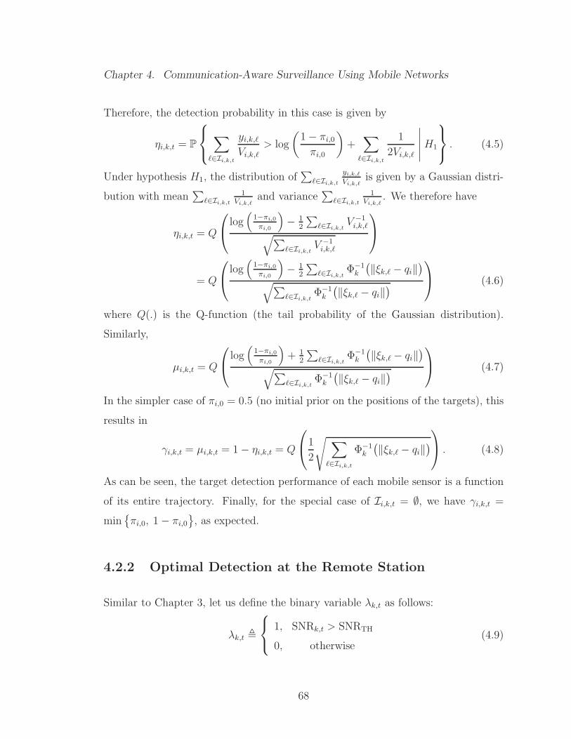
Chapter 4. Communication-Aware Surveillance Using Mobile Networks
Therefore, the detection probability in this case is given by
ηi,k,t = P
∑
ℓ∈Ii,k,t
yi,k,ℓVi,k,ℓ
> log
(1− πi,0πi,0
)+∑
ℓ∈Ii,k,t
1
2Vi,k,ℓ
∣∣∣∣∣H1
. (4.5)
Under hypothesis H1, the distribution of∑
ℓ∈Ii,k,tyi,k,ℓVi,k,ℓ
is given by a Gaussian distri-
bution with mean∑
ℓ∈Ii,k,t1
Vi,k,ℓand variance
∑ℓ∈Ii,k,t
1Vi,k,ℓ
. We therefore have
ηi,k,t = Q
log(
1−πi,0
πi,0
)− 1
2
∑ℓ∈Ii,k,t V
−1i,k,ℓ
√∑ℓ∈Ii,k,t V
−1i,k,ℓ
= Q
log(
1−πi,0
πi,0
)− 1
2
∑ℓ∈Ii,k,t Φ
−1k
(‖ξk,ℓ − qi‖
)
√∑ℓ∈Ii,k,t Φ
−1k
(‖ξk,ℓ − qi‖
)
(4.6)
where Q(.) is the Q-function (the tail probability of the Gaussian distribution).
Similarly,
µi,k,t = Q
log(
1−πi,0
πi,0
)+ 1
2
∑ℓ∈Ii,k,t Φ
−1k
(‖ξk,ℓ − qi‖
)
√∑ℓ∈Ii,k,t Φ
−1k
(‖ξk,ℓ − qi‖
)
(4.7)
In the simpler case of πi,0 = 0.5 (no initial prior on the positions of the targets), this
results in
γi,k,t = µi,k,t = 1− ηi,k,t = Q
1
2
√ ∑
ℓ∈Ii,k,t
Φ−1k
(‖ξk,ℓ − qi‖
) . (4.8)
As can be seen, the target detection performance of each mobile sensor is a function
of its entire trajectory. Finally, for the special case of Ii,k,t = ∅, we have γi,k,t =
minπi,0, 1− πi,0
, as expected.
4.2.2 Optimal Detection at the Remote Station
Similar to Chapter 3, let us define the binary variable λk,t as follows:
λk,t ,
1, SNRk,t > SNRTH
0, otherwise(4.9)
68

Chapter 4. Communication-Aware Surveillance Using Mobile Networks
Also, let τk,t denote the last time instant that the kth mobile sensor was connected
to the remote station, up to time t ≥ 1:
τk,t , max0 ∪ 1 ≤ ℓ ≤ t | λk,ℓ = 1
. (4.10)
Note that since t ≥ 1, we define τk,t = 0 to indicate the case that the kth mobile sensor
has not been yet connected to the remote station up to time t ≥ 1, i.e., λk,ℓ = 0 for
ℓ = 1, · · · , t. At any time instant, the remote station fuses the last received decisions
of all the mobile sensors (if available), regarding the presence of a target in a cell.
Let us define Ki,t as the set of the mobile sensors that have been connected to the
remote station at least once up to time t ≥ 1 and visited the ith cell at least once
before their last connection to the remote station.
Ki,t ,
1 ≤ k ≤ n
∣∣∣∣ qi ∈τk,t⋃
ℓ=1
Sk,ℓ, τk,t ≥ 1
. (4.11)
Assuming independent received observations from the mobile sensors, we then have
the following LRT at the remote station:4
∏
k∈Ki,t
Li,k,τk,t
xi,b,t=1≷
xi,b,t=0
1− πi,0πi,0
, (4.12)
where Li,k,τk,t denotes the LR corresponding to the last received observation from the
kth mobile sensor and is given by the following at any time 1 ≤ ℓ ≤ t:
Li,k,ℓ =p(xi,k,ℓ|H1)
p(xi,k,ℓ|H0)=
p(xi,k,ℓ=1|H1)
p(xi,k,ℓ=1|H0), xi,k,ℓ = 1
p(xi,k,ℓ=0|H1)
p(xi,k,ℓ=0|H0), xi,k,ℓ = 0
, (4.13)
where xi,k,ℓ denotes the decoded version of xi,k,ℓ at the remote station. We have
p(xi,k,ℓ = 1|H1)
p(xi,k,ℓ = 1|H0)
=p(xi,k,ℓ = 1|xi,k,ℓ = 1)p(xi,k,ℓ = 1|H1) + p(xi,k,ℓ = 1|xi,k,ℓ = 0)p(xi,k,ℓ = 0|H1)
p(xi,k,ℓ = 1|xi,k,ℓ = 1)p(xi,k,ℓ = 1|H0) + p(xi,k,ℓ = 1|xi,k,ℓ = 0)p(xi,k,ℓ = 0|H0)
=p(xi,k,ℓ = 1|xi,k,ℓ = 1)ηi,k,ℓ + p(xi,k,ℓ = 1|xi,k,ℓ = 0)(1− ηi,k,ℓ)
p(xi,k,ℓ = 1|xi,k,ℓ = 1)µi,k,ℓ + p(xi,k,ℓ = 1|xi,k,ℓ = 0)(1− µi,k,ℓ). (4.14)
4We implicitly assume that the remote station is aware of the sensing model of the mobilesensors and can calculate their corresponding detection and false-alarm probabilities, usingtheir instantaneous positions.
69

Chapter 4. Communication-Aware Surveillance Using Mobile Networks
Using the assumption of large SNRTH, the packets that are kept at the remote station
are error-free. Therefore, p(xi,k,ℓ = 1|xi,k,ℓ = 1) = 1 and p(xi,k,ℓ = 1|xi,k,ℓ = 0) = 0.
Then,p(xi,k,ℓ=1|H1)
p(xi,k,ℓ=1|H0)=
ηi,k,ℓµi,k,ℓ
. Similarly,p(xi,k,ℓ=0|H1)
p(xi,k,ℓ=0|H0)=
1−ηi,k,ℓ1−µi,k,ℓ
, which results in
Li,k,ℓ =
ηi,k,ℓµi,k,ℓ
, xi,k,ℓ = 1
1−ηi,k,ℓ1−µi,k,ℓ
, xi,k,ℓ = 0, (4.15)
Note that in case Ki,t = ∅, we have∏
k∈Ki,tLi,k,τk,t = 1. Then xi,b,t = 1 if πi,0 > 0.5,
and xi,b,t = 0 otherwise.
Detection, false-alarm and error probabilities at the remote station, as functions
of target detection performance of the mobile sensors and their channel to the remote
station, are also very important to characterize. Let ηi,b,t, µi,b,t and γi,b,t denote the
detection, false-alarm and error probabilities at the remote station, for detection of
a target in the ith cell at time t. We have
ηi,b,t = P
∏
k∈Ki,t
Li,k,τk,t >1− πi,0πi,0
∣∣∣∣∣H1
,
µi,b,t = P
∏
k∈Ki,t
Li,k,τk,t >1− πi,0πi,0
∣∣∣∣∣H0
,
γi,b,t = πi,0(1− ηi,b,t) + (1− πi,0)µi,b,t. (4.16)
Next, we show how to characterize these quantities.
4.2.3 Mathematical Characterization of the Performance at
the Remote Station
The trajectories of the mobile sensors affect both their sensing (target detection) and
communication qualities. In order to optimize the motion planning accordingly, we
need to mathematically characterize the impact of both on the probability of error
at the remote station. Let us define Bi,t ,b = [b1 · · · bn]T
∣∣ bk ∈ 0, 1, bk =
70

Chapter 4. Communication-Aware Surveillance Using Mobile Networks
0 ∀k 6∈ Ki,t
, with the size of |Bi,t| = 2|Ki,t|. This set contains all the possible binary
decisions of the mobile sensors of the ith cell, up to the last time they were connected
to the remote station (if k 6∈ Ki,t, then the kth mobile sensor will not cooperate in
the decision making process at the remote station). By calculating the probability
of occurrence of each member of Bi,t, under the both hypotheses H0 and H1, and
considering the cases where∏
k∈Ki,tLi,k,τk,t >
1−πi,0
πi,0, we get
ηi,b,t =∑
b∈Bi,t
[∏
k∈Ki,t
ηbki,k,τk,t(1− ηi,k,τk,t
)1−bk
]
×Heav
(∏
k∈Ki,t
(ηi,k,τk,tµi,k,τk,t
)bk(1− ηi,k,τk,t1− µi,k,τk,t
)1−bk
− 1− πi,0πi,0
),
µi,b,t =∑
b∈Bi,t
[∏
k∈Ki,t
µbki,k,τk,t
(1− µi,k,τk,t
)1−bk
]
×Heav
(∏
k∈Ki,t
(ηi,k,τk,tµi,k,τk,t
)bk(1− ηi,k,τk,t1− µi,k,τk,t
)1−bk
− 1− πi,0πi,0
), (4.17)
where Heav(.) denotes the Heaviside step function:
Heav(x) =
1, x > 0
0.5, x = 0
0, x < 0
(4.18)
Also, as explained previously, the detection error probability γi,b,t is calculated as
follows:
γi,b,t = πi,0(1− ηi,b,t) + (1− πi,0)µi,b,t. (4.19)
Similar to optimal detection at the mobile sensors, if Ki,t = ∅, we have γi,b,t =
minπi,0, 1 − πi,0
, as confirmed next. Using (4.17), we have ηi,b,t = µi,b,t =
Heav(1− 1−πi,0
πi,0
)= Heav (πi,0 − 0.5), for Ki,t = ∅. Therefore,
γi,b,t = πi,0 Heav (−πi,0 + 0.5) + (1− πi,0) Heav (πi,0 − 0.5) = minπi,0, 1− πi,0
.
(4.20)
71
Chapter 4. Communication-Aware Surveillance Using Mobile Networks
Furthermore, for the special case where πi,0 = 0.5 (no initial prior) and µi,k,τk,t =
1 − ηi,k,τk,t ,5 the detection error probability takes a more simplified form. First,
consider the following lemma:
Lemma 4.2.1. Let B denote the set of all the binary permutations of an n-dimensional
binary vector b. Assume ηk, for k = 1, · · · , n, denotes the probability that bk = 1.
Define
ηb =∑
b∈B
[n∏
k=1
ηbkk (1− ηk)1−bk
]Heav
(n∏
k=1
(ηk
1− ηk
)2bk−1
− 1
).
µb =∑
b∈B
[n∏
k=1
(1− ηk)bkη1−bk
k
]Heav
(n∏
k=1
(ηk
1− ηk
)2bk−1
− 1
). (4.21)
Then, ηb + µb = 1.
Proof. We have
ηb + µb =∑
b∈B
[n∏
k=1
ηbkk (1− ηk)1−bk
]
×[Heav
(n∏
k=1
(ηk
1− ηk
)2bk−1
− 1
)+Heav
(n∏
k=1
(1− ηkηk
)2bk−1
− 1
)]
=∑
b∈B
[n∏
k=1
ηbkk (1− ηk)1−bk
]= 1, (4.22)
where we used the fact that Heav(x− 1) + Heav( 1x− 1) = 1.
Using Lemma 4.2.1, we can immediately conclude that by setting 1 − ηi,k,τk,t =
µi,k,τk,t (for each mobile sensor) and1−πi,0
πi,0= 1 in (4.17), we have ηi,b,t = 1 − µi,b,t
(the same relationship between the detection and false-alarm probabilities hold at
the remote station). Therefore,
γi,b,t =∑
b∈Bi,t
[∏
k∈Ki,t
η1−bki,k,τk,t
µbki,k,τk,t
]Heav
(∏
k∈Ki,t
(ηi,k,τk,tµi,k,τk,t
)2bk−1
− 1
). (4.23)
5This is the case for several realistic sensing models, such as the Gaussian observationmodel introduced in Section 4.1.1.
72

Chapter 4. Communication-Aware Surveillance Using Mobile Networks
Similarly, for the case that Ki,t = ∅, (4.23) results in γi,b,t = 0.5.
The derived expressions for the performance at the remote station are useful
for the analysis purposes. However, their computational complexity makes them
improper choices for real-time motion planning applications. Next, we characterize
the Chernoff bound [87] on the probability of error at the remote station, which can
be calculated more efficiently and is a better choice for motion planning approaches
of Section 4.3.
4.2.4 Chernoff Bound On the Probability of Error at the
Remote Station
With the assumption of independent received observations from the mobile sensors,
the probability of detection error at the remote station is upper bounded by its
Chernoff bound as follows [87]: γi,b,t ≤ γi,b,t, where
γi,b,t = inf0<s<1
πsi,0
(1− πi,0
)1−s∏
k∈Ki,t
E
exp
(s log
(Li,k,τk,t
)) ∣∣∣H0
(4.24)
= inf0<s<1
πsi,0
(1− πi,0
)1−s∏
k∈Ki,t
[(ηi,k,τk,tµi,k,τk,t
)s
p(xi,k,τk,t = 1|H0)
+
(1− ηi,k,τk,t1− µi,k,τk,t
)s
p(xi,k,τk,t = 0|H0)
]
= inf0<s<1
πsi,0
(1− πi,0
)1−s∏
k∈Ki,t
[ηsi,k,τk,t µ
1−si,k,τk,t
+(1− ηi,k,τk,t
)s(1− µi,k,τk,t
)1−s].
Finding the optimum s in (4.24) is not easy in general. However, for the special
case of πi,0 = 0.5 and µi,k,τk,t = 1 − ηi,k,τk,t, the optimum exponent is s = 0.5, as
proved by the following lemma:6
6In case s = 0.5 is used, the Chernoff bound is called the Bhattacharyya bound [87].
73

Chapter 4. Communication-Aware Surveillance Using Mobile Networks
Lemma 4.2.2. Assume ηk > 0.5 for k ∈ K, where K ⊆ 1, · · · , n. Then,
argmin0<s<1
∏
k∈K
[ηsk (1− ηk)
1−s + η1−sk (1− ηk)
s]= 0.5. (4.25)
Proof. Define f(s) ,∑
k∈K log[ηsk (1− ηk)
1−s + η1−sk (1− ηk)
s]. Then, the optimum
s is the one that minimizes f(s) for s ∈ (0, 1). We have
d
dsf(s) =
∑
k∈K
ηsk (1− ηk)1−s log
(ηk
1−ηk
)− η1−s
k (1− ηk)s log
(ηk
1−ηk
)
ηsk (1− ηk)1−s + η1−sk (1− ηk)s
=∑
k∈Klog(αk)
(α2s−1k − 1
α2s−1k + 1
), (4.26)
where αk , ηk1−ηk
. It can be seen that ddsf(s) = 0 for s = 0.5, d
dsf(s) < 0 for
0 < s < 0.5 and ddsf(s) > 0 for 0.5 < s < 1, which completes the proof.
Using Lemma 4.2.2, the Chernoff bound, for the case of πi,0 = 0.5 (no initial prior)
and µi,k,τk,t = 1 − ηi,k,τk,t, is given by γi,b,t = 0.5∏
k∈Ki,t
[2√ηi,k,τk,t
(1− ηi,k,τk,t
) ].
Finally, in case Ki,t = ∅, the Chernoff bound on the probability of error will be
γi,b,t = inf0<s<1
πsi,0
(1 − πi,0
)1−s= min
πi,0, 1 − πi,0
, which is the same as what we
found previously for the probability of error in this case.
4.3 Motion Planning and PowerManagement Strate-
gies for Minimizing the Detection Error Prob-
ability at the Remote Station
Based on the explanations of the previous section, a communication-aware surveil-
lance problem in a mobile sensor network can be stated as follows: Given a lim-
ited operation time, T , limited average transmission powers for the mobile sensors,
PTX,AV,k, for k = 1, · · · , n, and their dynamical models, find the positions of the
74

Chapter 4. Communication-Aware Surveillance Using Mobile Networks
mobile sensors, ξk,t, as well as the instantaneous TX powers, PTX,k,t, for k = 1, · · · , nand over the entire time interval t = 1, · · · , T , such that one of the followings holds:
(i)∑T
t=1
∑mi=1 Eγi,b,t is minimized, while maximizing the probability of connec-
tivity of all the mobile sensors during the entire operation, i.e., Eλk,t, fork = 1, · · · , n and over the entire time interval t = 1, · · · , T .
(ii)∑m
i=1 Eγi,b,T is minimized, while maximizing the probability of connectivity
of the mobile sensors at the end of the operation, i.e., Eλk,T, for k = 1, · · · , n.
As explained before, problem (i) is applicable to the case where the remote sta-
tion requires a constant update on the target positions. Then, the mobile sensors are
required to maximize their probability of connectivity to the remote station during
the entire operation and improve their exploration performance within connectivity
constraints. In problem (ii), on the other hand, maximizing the probability of con-
nectivity during the entire operation is not a goal and the probability of error at the
end of the operation is the only performance measure. In this case, the mobile sensors
can freely explore the environment, provided that their probability of connectivity,
at the end of the operation, is maximized.
Solving problems (i) and (ii) is considerably challenging, without any approxi-
mation. Furthermore, the distribution of the channel at unvisited locations, which
is used to calculate Eγi,b,t, is time-varying. This makes solving the problem even
more challenging. Therefore, more efficient but approximate approaches are desired.
In this section, we propose a communication-aware motion planning framework
for suboptimally solving problems (i) and (ii). This is the main contribution of
this chapter. The proposed framework consists of two switching greedy approaches:
communication-constrained approach for problem (i) and hybrid approach for prob-
lem (ii). This framework can account for the time-varying distribution of channel
75

Chapter 4. Communication-Aware Surveillance Using Mobile Networks
variations, using a probabilistic assessment of wireless channels. We also introduce
robustness strategies, such as TX power adaptation, motion jittering and robustness
margins, to increase the robustness of the proposed framework to multipath fading
and channel assessment errors.7
Similar to Chapter 3, we use the channel assessment framework of Chapter 2 to
evaluate our proposed objective functions at unvisited locations. This is discussed in
more details when explaining the proposed motion planning approaches in the next
two sections.
4.3.1 Communication-Constrained Motion Planning
Consider planning the motion of the mobile sensors in order to constantly update
the remote station on the positions of the targets, while improving the exploration
performance of each individual mobile sensor. Assume πi,0 = 0.5 for 1 ≤ i ≤ m and
ηi,k,t = 1− µi,k,t for 1 ≤ i ≤ m and 1 ≤ k ≤ n. By using the optimal s = 0.5, we get
log(γi,b,t+1
)= log(0.5) +
∑
k∈Ki,t+1
log(2√ηi,k,τk,t+1
(1− ηi,k,τk,t+1
) ). (4.27)
Let KL(η) denote the Kullback-Leibler (KL) distance between two discrete distri-
butions Bern(0.5) and Bern(η), where Bern(η) represents the Bernoulli distribution
with the success probability of η. We have KL(η) = − log(2√η(1− η)
). Using the
definition of KL(η) and λk,t, we have
log(γi,b,t+1
)= log(0.5)−
n∑
k=1
[λk,t+1KL
(ηi,k,t+1
)+(1− λk,t+1
)KL(ηi,k,τk,t
)], (4.28)
where we set ηi,k,τk,t = 0.5 for τk,t = 0 (the case where the kth mobile sensor has
not yet been connected to the remote station up to time t ≥ 1). The average of
7Note that in this chapter, we are not concerned with energy conservation. Instead,our goal is to schedule a limited average TX power for communication. In case energyconservation is a goal, the current framework can be extended to consider communicationand motion powers and optimize the trajectories to minimize the total energy consumption.
76

Chapter 4. Communication-Aware Surveillance Using Mobile Networks
log(γi,b,t+1
), conditioned on the channel values up to time t, is then given by the
following:
E
log(γi,b,t+1
)∣∣∣λt= log(0.5)−
n∑
k=1
[Eλk,t+1
(KL(ηi,k,t+1
)−KL
(ηi,k,τk,t
))
+KL(ηi,k,τk,t
)], (4.29)
where λt = [λ1,1 · · · λn,t]T. Using the probabilistic channel assessment framework of
Chapter 2, the kth mobile sensor can assess the probability of being connected to the
remote station at time t+ 1 as follows:
Eλk,t+1
= P
GdB(ξk,t+1) > GdB,TH,k,t+1
= Q
(GdB,TH,k,t+1 − GdB,k,t,est(ξk,t+1)
σk,t,est(ξk,t+1)
),
(4.30)
where Q(.) is the Q-function, GdB,k,t,est(q) and σ2k,t,est(q) are the estimates of GdB,k,t(q)
and σ2k,t(q) respectively (see Theorem 2.2.2), with the exact channel parameters re-
placed by the estimated ones (similar to Chapter 3). Furthermore, GdB,TH,k,t+1 de-
notes the (possibly time-varying) channel power threshold of the kth mobile sensor
at time t+1 (in dB), which depends on the power management strategy that we in-
troduce in Section 4.4.1. We then propose the following decentralized greedy motion
optimization framework for the kth mobile sensor at time t, based on minimizing its
contribution to the average detection error probability of the next time step at the
remote station:
u∗k,t = argmaxuk,t
Jcc,k,t(ξk,t+1
), E
λk,t+1
︸ ︷︷ ︸Comm. obj.
[ m∑
i=1
KL(ηi,k,t+1)− Ck,t
]
︸ ︷︷ ︸Sensing obj.
s.t. 1) ξk,t+1 = ξk,t + uk,t, 2) ξk,t+1 ∈ Vk,t, (4.31)
where Ck,t ,∑m
i=1KL(ηi,k,τk,t
)is a constant (is not a function of ξk,t+1) and
Vk,t ,q ∈ W
∣∣∣ ‖q − ξk,t‖ ≤ umax,k,PGdB(q) > GdB,TH,k,t+1
≥ ∆conn
, (4.32)
77

Chapter 4. Communication-Aware Surveillance Using Mobile Networks
for a positive threshold ∆conn. Note that larger ∆conn will result in a more conserva-
tive (in terms of connectivity maintenance) but less sensing-effective strategy. This
threshold is chosen based on how much we need the communication-constrained ap-
proach to be robust to multipath fading (and other channel assessment errors). Also,
the sensing part of (4.31) is always non-negative as KL(ηi,k,t+1
)≥ KL
(ηi,k,τk,t
)for
every 1 ≤ i ≤ m.
Equation (4.31) is a key equation that shows 1) the separation of communication
and sensing objectives for the purpose of navigation, 2) that solely from a sensing
perspective, each mobile sensor should minimize its surveillance uncertainty at the
next step by maximizing its KL distance to Bern(0.5), 3) that solely from a commu-
nication perspective, each mobile sensor should maximize the probability of being
connected to the remote station at the next step and 4) that the optimal trajectory
is the one that provides the right balance between these objectives. In other words,
the optimal communication-constrained navigation strategy is the one that minimizes
the sensing uncertainty while maximizing the probability of being connected to the
remote station at the next step, based on what the mobile sensor can assess about the
connected regions.
One drawback of the localized motion planning strategy of (4.31) is its feasibility.
Based on the available knowledge on channel link qualities, there may be situations
where Vk,t = ∅ (for example the case where the mobile sensor starts in a disconnected
area far from the remote station). In such cases, the kth mobile sensor can get stuck in
a region with a poor link quality. Furthermore, even if the problem does not become
infeasible, if Area(Vk,t
)is too small, the proposed approach will be less robust to
channel assessment errors. In order to avoid such undesired conditions, next we
propose a switching strategy to navigate each mobile sensor to unvisited locations
with good link qualities, in case the link quality is poor in the local region around
the current position of the mobile sensor.
78

Chapter 4. Communication-Aware Surveillance Using Mobile Networks
A Switching Strategy for Avoiding Undesired Local Extrema
Let idx(q), for q ∈ W, denote the index of the cell that contains q, i.e., the unique i
such that q ∈ Wi. Also, let us define the following sets:
Ek,t ,q ∈ W
∣∣∣ PGdB(q) > GdB,TH,k,t+1
≥ ∆conn
,
Fk,t ,q ∈ W
∣∣∣ ηidx(q),k,t < ∆sens
, (4.33)
where ∆conn is as defined before and ∆sens is another positive threshold. The idea
behind the switching approach is to add another mode of operation, referred to as
the sensing-aware communication seeking mode, to navigate the kth mobile sensor
to the closest point in Ek,t ∩ Fk,t whenever∣∣Vk,t
∣∣ < εconn, for a small positive εconn.
Here,∣∣Vk,t
∣∣ represents the area of Vk,t. In other words, this mode navigates the kth
mobile sensor towards the closest unexplored (or poorly explored) region where the
probability of connection (using the current assessment of the channel at the mobile
sensor) is good enough. Then, as soon as we have∣∣Vk,t
∣∣ ≥ εconn, we switch back to
the motion planning strategy of (4.31), which we refer to as communication-aware
exploration mode. The control input of the kth mobile sensor in the sensing-aware
communication seeking mode can then be found as follows:
u∗k,t = argminuk,t
‖ξk,t+1 − q∗comm,k,t‖ (4.34)
s.t. 1) q∗comm,k,t = argminq∈Ek,t∩Fk,t
‖q − ξk,t‖, 2) ξk,t+1 = ξk,t + uk,t, 3) ‖uk,t‖ ≤ uk,max.
Using the control strategy of (4.34), whenever∣∣Vk,t
∣∣ < εconn, the kth mobile sensor
is navigated directly towards q∗comm,k,t, which is the closest point of Ek,t ∩ Fk,t to the
current position of the mobile sensor. Fig. 4.2 summarizes the proposed switching
strategy, which prevents the mobile sensor from getting stuck in undesired local ex-
trema. Furthermore, it increases the robustness to channel assessment errors (mainly
caused by multipath), by introducing extra design parameters such as ∆conn. In Sec-
79

Chapter 4. Communication-Aware Surveillance Using Mobile Networks
tion 4.4, we discuss more strategies for improving the performance and increasing
the robustness of the switching approach.
comm-aware
exploration
mode
|V | ≥ ε k,t conn
sens-aware
comm
seeking
mode
conn |V | < ε
k,t
Figure 4.2: Illustration of the proposed communication-constrained motion planning ap-proach.
4.3.2 Hybrid Motion Planning
Consider the communication-constrained motion planning approach of (4.31). The
communication part of the objective function in (4.31), i.e., the Q-function in the
definition of Jcc,k,t(ξk,t+1
), enforces the kth mobile sensor to move to the positions
with a higher chance of experiencing a better channel quality. As the quality of
channel learning gets better, σk,t,est(ξk,t+1) becomes smaller. In the limit of perfect
channel learning, the Q-function acts as a hard limiter, enforcing the mobile sensor to
only explore the connected regions. This property of the communication-constrained
approach can be considerably useful for the applications that require constant com-
munication of the most updated binary maps to the remote station, which requires
constant improvement of the probability of connection of individual mobile sensors.
However, for a limited operation time T and a time-invariant field, the mobile sensors
may only be concerned with the probability of detection error of the remote station
at the end of operation, i.e.,∑m
i=1 Eγi,b,T as explained before. Minimizing this will
result in a different motion planning approach, with a different balance between ex-
ploration and communication, which we refer to as hybrid motion planning. The idea
80

Chapter 4. Communication-Aware Surveillance Using Mobile Networks
behind the hybrid motion planning approach is to have each mobile sensor explore
the environment extensively and communicate its binary target map at the end of
the mission (note that the remote station only uses the last communication of each
mobile sensor). This proposed approach has four modes of operation:
• Mode 1 (sensing-aware exploration mode): In this mode, each mobile sensor
optimizes its motion only based on its sensing and exploration objectives, with-
out taking communication constraints into account. The purpose of this mode
is to explore the environment as much as possible, in the given operation time.
Each mobile sensor k, therefore, chooses its next motion decision such that its
local detection probability, ηi,k,t+1, is maximized. The controller input of the
kth mobile sensor is then calculated using the following optimization problem:
u∗k,t = argmaxuk,t
Jsens,k,t(ξk,t+1
),
m∑
i=1
ηi,k,t+1 (4.35)
s.t. 1) ξk,t+1 = ξk,t + uk,t, 2) ‖uk,t‖ ≤ umax,k, 3) ξk,t+1 ∈ W,
where the kth mobile sensor assesses its detection probability based on its sens-
ing model. In this mode, communication objectives are not considered in local
motion planning. However, it is possible that the mobile sensor transmits its
current decision vector if it randomly moves to a connected spot. This can
increase the robustness, in case the operation was terminated abruptly and
earlier than planned. However, from power consumption perspective, it may
be better if the mobile sensor does not communicate in this stage and leaves
all its power for optimizing the connectivity at the end of operation.
• Mode 2 (local extrema avoidance mode): Using the localized exploration strat-
egy of (4.35), each mobile sensor tries to explore the environment as much as
possible. However, there can be undesirable situations where it gets stuck in
a given area, while there are still unvisited areas that can be explored in the
81

Chapter 4. Communication-Aware Surveillance Using Mobile Networks
given operation time. Similar to the communication-constrained case, in or-
der to avoid such undesirable situations, we add a mode to navigate a mobile
sensor to poorly explored locations, whenever the estimated improvement of
its sensing quality is small. Using the definition of Fk,t in Section 4.3.1, the
mobile sensor switches to the local extrema avoidance mode, to move towards
the closest point in Fk,t, whenever
ψk,t ,maxξk,t+1∈Rk,t
∑mi=1 |ηi,k,t+1 − ηi,k,t|∑m
i=1 ηi,k,t< εsens, (4.36)
for a small positive εsens and Rk,t ,q ∈ W
∣∣ ‖q − ξk,t‖ ≤ umax,k
. In other
words, we navigate the mobile sensor towards the closest poorly explored point
in the workspace in order to improve its sensing performance. We then switch
back to the sensing-aware exploration mode as soon as we have ψk,t ≥ εsens. The
control input of the kth mobile sensor, in this mode, is also found by following
the same approach of the sensing-aware communication seeking mode of the
previous case:
u∗k,t = argminuk,t
‖ξk,t+1 − q∗sens,k,t‖ (4.37)
s.t. 1) q∗sens,k,t = argminq∈Fk,t
‖q − ξk,t‖, 2) ξk,t+1 = ξk,t + uk,t, 3) ‖uk,t‖ ≤ uk,max.
• Mode 3 (connection-seeking mode): Once the environment is explored exten-
sively and the limited operation time is approaching, each mobile sensor needs
to move to positions with high chance of connectivity, where it can send its
most updated binary decision vector to the remote station. Based on its most
recent predicted channel, each mobile sensor has an estimate of how many steps
it takes for it to move to a connected position. Based on this knowledge and
by considering the remaining number of operation steps, each mobile sensor
can decide when to switch from the sensing-aware exploration mode or the
local extrema avoidance mode to the connection-seeking mode. Consider the
82

Chapter 4. Communication-Aware Surveillance Using Mobile Networks
set Ek,t, defined in Section 4.3.1. The closest point in Ek,t is then found as fol-
lows: q∗seek,k,t = argminq∈Ek,t
‖q − ξk,t‖. Using the fist-order dynamics of the mobile
sensors, the minimum number of steps required to get to q∗seek,k,t, at time t, is
ζk,t =⌊‖ξk,t−q∗seek,k,t‖
umax,k
⌋+ 1. The kth mobile sensor switches to the connection-
seeking mode at time t if 1) it is not connected to the remote station at time
t and 2) ζk,t ≥ T − t −M , where M is a positive and small offset, which can
add a robustness margin to the operation. Once a decision to switch to the
connection-seeking mode is made, the control input of each mobile sensor is
found as follows:
u∗k,t = argminuk,t
‖ξk,t+1 − q∗seek,k,t‖ (4.38)
s.t. 1) q∗seek,k,t = argminq∈Ek,t
‖q − ξk,t‖, 2) ξk,t+1 = ξk,t + uk,t, 3) ‖uk,t‖ ≤ uk,max.
Similar to the communication-constrained approach, as we increase ∆conn in
Ek,t, the motion planner becomes more robust to the variations of multipath
fading and other assessment uncertainties, by acting more conservatively.
• Mode 4 (communication-aware exploration mode): Once a mobile sensor moves
to a region where∣∣Vk,t
∣∣ ≥ εconn, it utilizes the proposed communication-aware
exploration mode of Section 4.3.1, in order to maintain its connectivity to
the remote station till the end of operation. In this mode, the mobile sensor
still senses the connected area, as described in the previous section. However,
its main goal is connectivity maintenance. Note that in case the kth mobile
sensor is still disconnected after switching to this mode (possibly due to its poor
assessment of the channel in the presence of large multipath fading), it can take
advantage of a jittery movement around its current location, in order to increase
its chance of connectivity. In the next section, we explain such strategies to
further increase the robustness of both communication-constrained and hybrid
approaches.
83

Chapter 4. Communication-Aware Surveillance Using Mobile Networks
Fig. 4.3 demonstrates an overview of the hybrid approach where transition between
the modes is illustrated.
sensing-
aware
exploration
mode
local extrema
avoidance
mode
comm
seeking
mode
comm-aware
exploration
mode
ζ ≥ T − t − M k,t
ζ ≥ T − t− M k,t
ψ ≥ ε k,t sens ψ < ε
k,t
conn
sens
|V | ≥ ε k,t
Figure 4.3: Illustration of the proposed hybrid motion planning approach.
4.4 Further Robustness to Multipath Fading and
other Channel Assessment/Modeling Errors
In Chapter 2, we explained how our probabilistic channel assessment framework can
be used by each mobile sensor to learn the shadowing and path loss components and
characterize the channel learning uncertainty, in the presence of multipath fading
and other channel assessment errors. This enabled our probabilistic motion con-
trol approaches in Section 4.3.1 and 4.3.2. We also showed how to increase the
robustness, by introducing a number of design parameters (such as ∆conn). In this
section, we discuss more strategies to increase the robustness to multipath fading
and other channel assessment/modeling errors. These strategies can be combined
with our communication-constrained or hybrid motion planners to further improve
the performance. Fig. 4.4 summarizes how our proposed framework handles different
84

Chapter 4. Communication-Aware Surveillance Using Mobile Networks
elements of wireless channels using 1) probabilistic assessment of the shadowing and
path loss components and 2) strategies to increase robustness to multipath fading and
other modeling errors. We will discuss the robustness strategies in the subsequent
sections.
Figure 4.4: Illustration of the proposed probabilistic channel assessment framework androbustness techniques.
4.4.1 Adaptive Transmit Power and Packet Dropping Thresh-
old for Increasing the Robustness to Multipath Fading
The threshold GdB,TH,k,t+1 in the formulation of Eλk,t+1 in (4.30), as well as in
the definitions of Vk,t and Ek,t, depends on the TX power adaptation strategy of the
kth mobile sensor. Consider the case where the kth mobile sensor is given the total
average TX power of PTX,AV,k. It can use the fixed TX power of PTX,k,t = PTX,AV,k
during its operation, independent of the channel quality. In this case, we have
GdB,TH,k,t+1 = 10 log10
(SNRTHBN0
PTX,AV,k
)+ ∆GdB,TH, where ∆GdB,TH ≥ 0 is added to
increase the robustness to multipath fading. The idea is that by increasing the
packet-dropping threshold, the mobile sensor is then forced to operate in regions
with higher channel power, resulting in more robustness to multipath fading.
85

Chapter 4. Communication-Aware Surveillance Using Mobile Networks
Alternatively, each mobile sensor can adapt its TX power to channel quality.
Power adaptation strategies have been heavily explored in the communication litera-
ture [45,46,101]. In this chapter, the goal of TX power adaptation is to increase the
robustness of the proposed motion planning algorithm by saving power at positions
with high channel qualities, with the goal of satisfying the connectivity requirements
at positions with low channel qualities. Similar to [101], we consider the following
simple TX power adaptation strategy for each mobile sensor:
PTX,k,t =
0, min(PTX,AV,k,t, PTX,max,k
)< SNRTHBN0
G(ξk,t)
SNRTHBN0
G(ξk,t), otherwise
, (4.39)
where PTX,max,k is the maximum TX power of the kth mobile sensor and PTX,AV,k,t is
the average of the remaining power budget of the kth mobile sensor at time instant
t:
PTX,AV,k,t =1
T − t+ 1
(TPTX,AV,k −
t−1∑
ℓ=1
PTX,k,ℓ
). (4.40)
Based on (4.39), the kth mobile sensor sends its binary decision vector to the
remote station at time t when the minimum required TX power to make the mobile
sensor connected is no larger than min(PTX,AV,k,t, PTX,max,k
). The channel power
threshold is then selected to be:
GdB,TH,k,t+1 = 10 log10
(SNRTHBN0
min(PTX,AV,k,t, PTX,max,k)
)+∆GdB,TH. (4.41)
Note that in this chapter, we are not concerned with minimizing the total energy
consumption. In other words, our goal is to schedule a limited average TX power for
communication. However, the current framework can be extended to consider both
communication and motion powers and optimize the trajectories of the mobile sensors
such that the total energy consumption is minimized, while the main networked task
is accomplished. It is also worth mentioning that, in the hybrid approach, the mobile
86

Chapter 4. Communication-Aware Surveillance Using Mobile Networks
sensors may decide not to send anything, while operating in modes 1 and 2, to save
power for the end of the operation when they need to be connected. This strategy
is particularly useful for long operations with limited power budgets. However, if
power is not a constraint, the mobile sensors can always send their most updated
target maps to the remote station if they move to a connected spot by chance. This
can further increase the robustness, in case the operation terminates abruptly and
earlier than planned.
4.4.2 Jittery Movements for Increasing the Probability of
Connectivity in the Presence of Large Multipath Fad-
ing
Consider the communication-constrained approach. This strategy guides each mobile
sensor to an area that has a high probability of connectivity. However, a specific
position may or may not have the connectivity requirement, as our channel learning
framework cannot predict the fine variations of multipath fading and is also prone
to errors. Since the mobile sensor is guided to an area that has a high probability of
connectivity (high average channel power), then small jittering can help the mobile
sensor find a better location in terms of connectivity. In case a jittery movement is
added, after the proposed communication-constrained or hybrid motion planner is
executed at each step, the mobile sensor picks Njitt random points in a small circular
region around its current location. It then moves to each point one by one, measures
the channel there, and then simply chooses the point with the best channel quality
for sending. The radius of the circular region for jittering is chosen such that the
path loss and shadowing parts of channel remain stationary in the region, based on
the assessment of the channel available to each mobile sensor. Note that in case the
adaptive TX power strategy of (4.39) is used, if none of the Njitt points satisfy the
87

Chapter 4. Communication-Aware Surveillance Using Mobile Networks
the connectivity requirement at some steps, nothing will be sent.
4.5 Performance Analysis of the Proposed Motion
Planning Strategies
With some assumptions, it is possible to analyze the final performance of the pro-
posed communication-constrained and hybrid approaches. The following theorems
summarize our key results:
Theorem 4.5.1. Assume that 1) the mobile sensors use the fixed TX power strategy
of PTX,k,t = PTX,AV,k, for k = 1, · · · , n, 2) based on the assessment of the channel
at all the mobile sensors, W \ ∪∞t=1 ∪n
k=1 Ek,t 6= ∅ (refer to Section 4.3.1 for the
definition of Ek,t), and 3) the sensing radius of each mobile sensor and the size of
each cell are small, compared to the size of the workspace, such that some of the cells
in W \∪∞t=1 ∪n
k=1 Ek,t cannot be sensed by any mobile sensor k, while it moves inside
∪∞t=1Ek,t. Then, the average of the probability of error at the remote station in the
communication-constrained approach (averaged over the space and the conditional
distribution8 of the channel) is lower bounded by a positive value at any time, i.e.,
there exists γ > 0 such that 1m
∑mi=1 E
γi,b,t
≥ γ, for all k ≥ 1.
Proof. For every t ≥ 1, we have
1
m
m∑
i=1
Eγi,b,t
≥ 1
m
m∑
i=1
Eγi,b,T
≥ lim
T→∞
1
m
m∑
i=1
Eγi,b,T
, (4.42)
where the expected values are calculated over the conditional distribution of the
channel. Assuming πi,0 = 0.5, for 1 ≤ i ≤ m, and ηi,k,t = 1 − µi,k,t, for 1 ≤ i ≤ m
8The distribution of the channel conditioned on the finite set of channel measurements.
88

Chapter 4. Communication-Aware Surveillance Using Mobile Networks
and 1 ≤ k ≤ n, we obtain
limT→∞
γi,b,T =∑
b∈B
[n∏
k=1
(1− µi,k,∞)1−bk µbki,k,∞
]Heav
(n∏
k=1
(1− µi,k,∞µi,k,∞
)2bk−1
− 1
),
(4.43)
where µi,k,∞ , limT→∞ µi,k,τk,T and B is the set of all the binary vectors of size
n. Note that µi,k,∞ = 0.5 in case limT→∞ τk,T = 0. Consider the communication-
constrained approach, where PTX,k,t = PTX,AV,k and W \ ∪∞t=1 ∪n
k=1 Ek,t 6= ∅. If the
sensing radius of each mobile sensor and the size of each cell are small, we can find
some cell i inside W \∪∞t=1 ∪n
k=1 Ek,t 6= ∅ and some µi> 0, such that µi,k,∞ ≥ µ
i, ∀k.
This cell i can be any cell inside W\∪∞t=1∪n
k=1Ek,t, which is not visited by any mobile
sensor during the entire operation or is sensed for a finite number of steps before each
mobile sensor reaches Ek,t, for k = 1, · · · , n. This implies that there exists a positive
lower bound on limT→∞1m
∑mi=1 γi,b,T and, by averaging over the conditional channel
distribution, on limT→∞1m
∑mi=1 E
γi,b,T
. In other words, there exists γ > 0 such
that limT→∞1m
∑mi=1 E
γi,b,T
≥ γ. The same result can be obtained for the more
general case where πi,0 6= 0.5, for some 1 ≤ i ≤ m, or ηi,k,t 6= 1 − µi,k,t, for some
1 ≤ i ≤ m and 1 ≤ k ≤ n, using (4.17). This completes the proof.
Theorem 4.5.2. Assume that 1) the channel is assessed perfectly,9 2) the mobile
sensors are connected to the remote station at the beginning of the operation, 3) the
sensing radius of each mobile sensor and the size of each cell are small, compared to
the size of the workspace, such that the maximum area covered by a mobile sensor
k, while moving in Ek,t, is approximately equal to the area of Ek,t (refer to Section
4.3.1 for the definition of Ek,t), for k = 1, · · · , n, 4) the mobile sensors use the
same fixed TX power strategy of PTX,k,t = PTX,AV, for k = 1, · · · , n, 5) πi,0 =
9By this assumption we automatically assume that the multipath fading power is zero,the channel parameters are estimated perfectly and the number of channel measurementsin the environment are large such that σk,t(q) → 0 for all k, q ∈ W and t ≥ 1. SeeDefinition 3.2.1 in Chapter 3 for more details.
89

Chapter 4. Communication-Aware Surveillance Using Mobile Networks
0.5, for i = 1, · · · , m, and 6) the workspace is a circular region with the remote
station located at the center of the circle. Then, in the communication-constrained
approach, a lower bound for limT→∞1m
∑mi=1 E
γi,b,T
(averaged over every possible
channel) is approximately given by 0.5[Q(a) − exp
(2+2aρρ2
)Q(
2+aρρ
)], where a =
KdB−10nPL log10(RW )−GdB,TH
ϑ, ρ = 10nPL
ϑ log(10), GdB,TH = 10 log10
(BN0SNRTH
PTX,AV
)and RW is the
radius of the workspace.
Proof. In case the mobile sensors start connected and the channel is assessed per-
fectly, each mobile sensor k only explores Ek,t in the communication-constrained
approach. Then, if there exists only one connected region around the remote station
and the size of the cells and the sensing radii of the mobile sensors are small, we
approximately have
limT→∞
1
m
m∑
i=1
γi,b,T ≥∣∣W \ ∪∞
t=1 ∪nk=1 Ek,t
∣∣2∣∣W∣∣ . (4.44)
In case of perfect channel assessment, the area ofW\∪∞t=1∪n
k=1Ek,t is equal to the areaof the disconnected region. Therefore, by averaging over the channel distribution,
we get
limT→∞
1
m
m∑
i=1
Eγi,b,T
≥ 0.5
πR2W
∫
WPGdB(q) < GdB,TH
dq
=1
R2W
∫ RW
0
rQ
(KdB − 10nPL log10(r)−GdB,TH
ϑ
)dr
= 0.5
[Q(a)− exp
(2 + 2aρ
ρ2
)Q
(2 + aρ
ρ
)], (4.45)
for ρ = 10nPL
ϑ log(10), a =
KdB−10nPL log10(RW )−GdB,TH
ϑand GdB,TH = 10 log10
(BN0SNRTH
PTX,AV
),
where we used the method of Chapter 2 of [59] to calculate the integral.
Theorem 4.5.3. Assume that the channel is assessed perfectly, πi,0 = 0.5, for 1 ≤i ≤ m, and ηi,k,t = 1− µi,k,t, for 1 ≤ i ≤ m and 1 ≤ k ≤ n. In the hybrid approach,
if we select ∆sens = 1− δsens (see Section 4.3.1 for the definition of the ∆sens), for an
90

Chapter 4. Communication-Aware Surveillance Using Mobile Networks
arbitrary small positive δsens, then we have the following for the asymptotic average
probability of detection error at the remote station: limT→∞1m
∑mi=1 E
γi,b,T
≤ δsens,
where averaging is done over every possible channel.
Proof. Assume that the mobile sensors start with the sensing-aware exploration mode
in the hybrid approach. Consider the kth mobile sensor, for 1 ≤ k ≤ n. For this
mobile sensor, the exploration continues (the spatial average of its detection error
probability decreases) until ψk,t < εsens (see Section 4.3.2 for the definition of the
variables). In this case, we have either Fk,t = ∅, which means that µi,k,t ≤ δsens, for
1 ≤ i ≤ m, or Fk,t 6= ∅. For the latter, the proposed local extrema avoidance mode
of the hybrid approach navigates the mobile sensor to a point in Fk,t. Then, two
different cases may happen. If a situation where ψk,t ≥ εsens does not happen, while
in the local extrema avoidance mode, the mobile sensor will remain in this mode
and visit every point in Fk,t until Fk,t = ∅. On the other hand, if the mobile sensor
switches back to the sensing-aware exploration mode at some point, the exploration
continues similar to the previous case, which also proves that Fk,t = ∅ after some
steps. Therefore, we have µi,k,t ≤ δsens, for 1 ≤ i ≤ m and t greater than a positive
constant. Then, assuming that the channel is assessed almost perfectly, we have
µi,k,∞ ≤ δsens (see the proof of Lemma 4.5.1 for the definition of µi,k,∞), for 1 ≤ i ≤ m
and 1 ≤ k ≤ n. This implies that limT→∞ γi,b,T ≤ δsens, for 1 ≤ i ≤ m. By averaging
over the channel distribution, we have limT→∞ Eγi,b,T
≤ δsens, for 1 ≤ i ≤ m,
which completes the proof.
As indicated by Theorem 4.5.3, the hybrid approach almost always outperforms
the communication-constrained one, in terms of the final probability of error at
the remote station, for large enough T . We compare the performance of the two
approaches in the next section, using both simulated and experimental data.
91

Chapter 4. Communication-Aware Surveillance Using Mobile Networks
4.6 Simulation and Experimental Results
In this section, we evaluate the performance of the proposed communication-aware
surveillance framework using both simulated and real channel measurements. Our
results highlight the underlying trade-offs in the design space as summarized later in
this section. For instance, they show that while the hybrid approach outperforms the
communication-constrained one in terms of the final probability of networked detec-
tion error, the latter has a higher probability of constant connectivity and is therefore
more robust to the abrupt termination of the operation. Also, we further compare
these two approaches with communication-unaware strategies (strategies that con-
sider only sensing objectives for planning the motion of the mobile sensors) and show
the effectiveness of the proposed framework in realistic fading environments.
Consider a surveillance scenario where three mobile sensors are tasked to explore
a given environment for the possible presence of targets. We use the Gaussian obser-
vation model of Section 4.1.1, where the following form is chosen for the observation
error variance [17, 73]:
Φk(d) =
d2 + ν, d < dsen
∞, otherwise(4.46)
for positive constants > 0 and ν > 0 and a limited sensing radius dsen for each mo-
bile sensor. The communication channel between the mobile sensors and the remote
station is simulated using our probabilistic channel simulator, which can simulate
path loss, shadow fading and multipath fading, with realistic spatial correlations. A
detailed description of this channel simulator can be found in [54, 56].
First we compare the trajectories of communication-constrained and hybrid plan-
ning approaches, for a fixed TX power case, where the following parameters are used:
umax,k = 3.0 m for k = 1, 2, 3, = 0.02, ν = 0.04, dsen = 3.0 m, KdB = −10 dB,
nPL = 2.5, ϑ = 2 dB, β = 4 m, ω = 2 dB, BN0 = −85 dB, PTX,AV,k = −20 dB, for
92

Chapter 4. Communication-Aware Surveillance Using Mobile Networks
k = 1, 2, 3, PTX,max,k = −10 dB, for k = 1, 2, 3, and SNRTH = 23 dB, with a Rician
multipath fading. Note that Rician multipath fading was simulated to make the
simulated more realistic. Furthermore, we use the following design parameters when
implementing our communication-aware and hybrid motion planners: ∆conn = 0.8,
∆sens = 0.65, εconn = 0.25, εsens = 0.002, ∆GdB,TH = 0 and M = 5 (see Section 4.3.1
and 4.3.2 for the definition of these parameters). For the purpose of channel learning,
the mobile sensors use 0.01% of the total channel samples (64 samples in a 800×800
grid), which are assumed to be randomly collected during an initial learning phase.
Then, they collect more samples as they move along their trajectories. The collected
samples are used to estimate the underlying channel parameters and assess the spa-
tial variations of the channel at unvisited areas. Fig. 4.5 shows the trajectories of the
mobile sensors for one simulated channel in both cases. The black regions in Fig. 4.5
represent the areas where the mobile sensors are not connected to the remote station
(received SNR is below the acceptable threshold), given PTX,k,t = PTX,AV,k. It can
be seen that by using the communication-constrained approach, the mobile sensors
converge to the regions where they are connected to the remote station (if they are
not connected at the beginning) and stay connected afterwards. In other words, this
approach forces the mobile sensors to mostly explore the regions with better link
qualities, so that they can constantly update the remote station and minimize its
detection error probability, as we explained in Section 4.3.1. The hybrid navigation
strategy, on the other hand, allows the mobile sensors to explore the environment
more freely. It, however, enables the mobile sensors to be connected to the remote
station at the end of operation. Also, as can be seen from the figure, some regions
may be revisited by the mobile sensors several times along their trajectories. Note
that in both cases, the mobile sensors take advantage of a jittery movement, in areas
of radius 0.3 m around their current locations and by testing Njitt = 45 points at each
step. In this specific example, jittery movement in the communication-constrained
case results in 10%, 15% and 17% increase in the percentage of time that Mobile
93

Chapter 4. Communication-Aware Surveillance Using Mobile Networks
Sensor #1, Mobile Sensor #2 and Mobile Sensor #3 are connected along their trajec-
tories, respectively. Similarly, in the hybrid approach, by using the jittery movement
we have 24%, 20% and 41% increase in the percentage of time that Mobile Sensor
#1, Mobile Sensor #2 and Mobile Sensor #3 are connected along their trajectories,
respectively.
−20 −10 0 10 20−20
−15
−10
−5
0
5
10
15
20
X (m)
Y (
m)
−20 −10 0 10 20−20
−15
−10
−5
0
5
10
15
20
X (m)
Y (
m)
Figure 4.5: Trajectories of three mobile sensors for communication-constrained (left) andhybrid (right) cases, with fixed TX powers. The red, magenta and green lines correspondto the trajectories of the Mobile Sensor #1, Mobile Sensor #2 and Mobile Sensor #3,respectively. The empty boxes and the filled ones denote the initial and final positionsrespectively. The location of the remote station is denoted on the top left corner of thefigures. See the pdf file for more visual clarity.
Next, consider the case where the adaptive TX power strategy of (4.39) is used for
both communication-constrained and hybrid approaches.10 Then, the connectivity
regions will become time-varying and different for different mobile sensors (since
their TX powers are different). One would expect that the white regions (connectivity
regions), corresponding to the kth mobile sensor, expand as its instantaneous average
10As explained before, in case energy conservation is not an issue, a mobile sensor cantransmit any time it is connected by luck in the hybrid approach too and hence apply theadaptive TX power strategy of (4.39). Multiple transmissions (as opposed to transmissiononly at the end of the operation) in the hybrid case will increase the robustness, althoughit is not required.
94

Chapter 4. Communication-Aware Surveillance Using Mobile Networks
TX power, PTX,AV,k,t, increases. Fig. 4.6 shows the evolution of the connectivity
regions for both strategies, for one of the mobile sensors of Fig. 4.5, when the TX
power adaptation technique of (4.39) is used. The communication channel is taken to
be the same as the one used in Fig. 4.5. In such an adaptive strategy, the connectivity
region of the mobile sensor expands with time with high probability, as can be seen
from the figure, for two reasons. First, in case of poor channel quality at time t, the
mobile sensor does not send anything, which results in an increase in PTX,AV,k,t+1 and
an expansion in its next step connectivity region. Second, in case the mobile sensor
decides to send its updated target map to the remote station using (4.39), it uses
the minimum required power for connectivity, given by SNRTHBN0
G(ξk,t), using its measured
channel power at time t. Note that we did not simulate any jittery movement in this
case.
−20 −10 0 10 20−20
−15
−10
−5
0
5
10
15
20
X (m)
Y (
m)
−20 −10 0 10 20−20
−15
−10
−5
0
5
10
15
20
X (m)
Y (
m)
−20 −10 0 10 20−20
−15
−10
−5
0
5
10
15
20
X (m)
Y (
m)
−20 −10 0 10 20−20
−15
−10
−5
0
5
10
15
20
X (m)
Y (
m)
−20 −10 0 10 20−20
−15
−10
−5
0
5
10
15
20
X (m)
Y (
m)
−20 −10 0 10 20−20
−15
−10
−5
0
5
10
15
20
X (m)
Y (
m)
−20 −10 0 10 20−20
−15
−10
−5
0
5
10
15
20
X (m)
Y (
m)
−20 −10 0 10 20−20
−15
−10
−5
0
5
10
15
20
X (m)
Y (
m)
Figure 4.6: Impact of the adaptive TX power on connectivity regions. Time-varyingconnectivity regions (white areas) in communication-constrained (top row) and hybrid(bottom row) cases are shown for one of the mobile sensors of Fig. 4.5, at time stepst = 15, t = 25, t = 35 and t = 45 (from left to right). The communication channel is takento be the same as the one used in Fig. 4.5. Empty boxes and filled ones denote the initialand final positions respectively. See the pdf file for more visual clarity.
In order to further compare the communication-constrained and hybrid approaches,
Fig. 4.7 (left) shows the average of the final detection error probability at the remote
95

Chapter 4. Communication-Aware Surveillance Using Mobile Networks
station, i.e., 1m
∑mi=1 Eγi,b,T, as a function of the given operation time T , for the
three mobile sensors and the same system parameters of Fig. 4.5.11 The averaging
is done over the space and 20 different channels. In Fig. 4.7 (left), for every T , the
whole trajectory of the mobile sensor is generated for 20 different channels and the
average results at the end of the operation are then plotted. In order to simplify
the scenario, TX power is not adaptive in this case and the mobile sensors, in both
communication-constrained and hybrid approaches, use the constant TX power of
PTX,AV,k = −20 dB at each step. They, however, make use of a jittery movement, at
the end of each step, to increase their chance of connectivity to the remote station.
It can be seen that the hybrid approach outperforms the communication-constrained
one, in terms of the average of the final detection error probability at the remote
station, as expected. The figure also shows that as T → ∞, the average prob-
ability of error goes to zero in the hybrid case, while it reaches an error floor in
the communication-constrained case. However, the communication-constrained ap-
proach provides smaller average detection error probability at the remote station, in
case the operation terminates earlier than the planned time T . To see this, Fig. 4.7
(right) shows the average of the detection error probability at the remote station, i.e.,
1m
∑mi=1 Eγi,b,t, as a function of time step t, averaged over space and 20 different
channels. We used T = 50 as the operation time in this case. As can be seen, if the
operation ends while the hybrid approach is still in the exploration mode, it results
in a worse performance, as it is designed to optimize the operation given a certain
time.
Fig. 4.8 compares the performance of three approaches, with different levels of
awareness, in terms of communication and sensing, for the same system parameters of
Fig. 4.5. The results are averaged over 20 different channels. Similar to Fig. 4.7, TX
power is not adaptive. Also, no jittery movement is simulated in this case, to show
11The spatial average or spatial integration of the quantity under control, is a popularchoice for the performance measure in surveillance and exploration literature [17].
96

Chapter 4. Communication-Aware Surveillance Using Mobile Networks
10 20 30 40 50 600
0.05
0.1
0.15
0.2
0.25
0.3
0.35
0.4
total number of steps (T)
av
era
ge
of
the
fin
al
de
t. e
rr.
pro
b.
at
the
RS
Comm−constrained
Hybrid
10 20 30 40 500
0.1
0.2
0.3
0.4
0.5
time step (t)
avera
ge o
f th
e d
et.
err
. p
rob
. at
the R
S
Comm−constrained
Hybrid
Figure 4.7: Average of the detection error probability at the remote station (RS) as afunction of (left) the given operation time (T ) and (right) time step (t) for communication-constrained and hybrid approaches. TX power is not adaptive in this case.
the underlying trade-off more clearly. For the sake of comparison, the results for a
sensing-constrained case are also shown. A sensing-constrained case only optimizes
the exploration objective and communicates with the remote station anytime its
trajectory takes it to the connected regions, as was described in modes 1 and 2
of the hybrid case. Thus, it is unaware of communication objectives. The figure
shows the average of the final detection error probability at the remote station, as
a function of SNRTH, for two cases of T = 10 (left) and T = 50 (right). Interesting
trade-offs can be observed. Consider the left figure, where T is small. In this case,
as SNRTH increases, the chance of connectivity becomes small over the whole space.
As such, the performance of the sensing-constrained approach degrades considerably,
for large SNRTH, since it does not include communication objectives in its motion
optimization. It can be see that the communication-constrained and hybrid cases
perform almost the same and better than the sensing constrained approaches. Also,
in this case, the average of the detection error probability in the communication-
constrained and hybrid approaches are large (compared to detection error probability
of hybrid approach in the right figure). This is because the operation time is limited
and the requirement on link qualities is high. The right figure, on the other hand,
shows the performance for the case of T = 50. In this case, since the given operation
97

Chapter 4. Communication-Aware Surveillance Using Mobile Networks
time is longer than the left figure, the trajectory of the sensing-constrained approach
crosses through more connected regions by luck, which improves its performance. For
the communication-constrained case, the performance degrades as SNRTH increases
since its exploration is limited to connected regions, which are shrinking as SNRTH
increases. The hybrid approach, however, results in the best performance in both
cases, providing the best trade-off between sensing and communication, as expected.
18 20 22 24 260.25
0.3
0.35
0.4
0.45
0.5
SNRTH
(dB)
av
era
ge
of
the
fin
al
de
t. e
rr.
pro
b.
at
the
RS
Comm−constrained
Hybrid
Sensing−constrained
18 20 22 24 260.05
0.1
0.15
0.2
0.25
0.3
0.35
0.4
0.45
SNRTH
(dB)
av
era
ge
of
the
fin
al
de
t. e
rr.
pro
b.
at
the
RS
Comm−constrained
Hybrid
Sensing−constrained
Figure 4.8: Communication and sensing trade-offs in a networked surveillance scenario.The figure shows average of the final detection error probability at the remote station (RS),averaged over the space and channel distribution, as a function of SNRTH, for two cases ofT = 10 (left) and T = 50 (right).
In order to show the performance of our framework with real channel measure-
ments, Fig. 4.9 shows a surveillance scenario, using one mobile sensor and by con-
sidering the real channel measurements gathered in the basement of our building.
The channel measurements are collected through a survey of the channel, using the
onboard IEEE 802.11g WLAN card of a Pioneer 3-AT robot (shown in Fig. 4.11) and
for a remote station (an IEEE 802.11g wireless router) located in one of the rooms
in the basement. This channel samples are then used to simulate the surveillance
scenario. During the surveillance operation, the channel is assessed based on 0.1%
a priori channel samples (47 samples), as well as the samples the mobile sensor col-
lects along its trajectory. The TX power is kept fixed and a received SNR threshold
of 35 dB is chosen for packet dropping. The mobile sensor also takes advantage of
a jittery movement, in areas of radius 0.15 m around its current locations and by
98

Chapter 4. Communication-Aware Surveillance Using Mobile Networks
testing Njitt = 20 points at each step. The sensing model is the same as the one
used for the previous simulations, except that we use dsen = 1.0 m in this case. The
Pioneer robot is modeled by the holonomic dynamical model of this chapter, with
umax,k = 1.5. A simple obstacle avoidance strategy, similar to the one proposed in [6],
is also used. The left and right figures in Fig. 4.9 show the trajectory of the mobile
sensor in the communication-constrained and hybrid approaches respectively, where
the true connectivity map to the remote station is superimposed on the blueprint of
the basement. Fig. 4.10 then compares the resulting average of the detection error
probability at the remote station, as a function of time step t.
It can be seen that, although multipath fading power is large, the mobile sen-
sor maintains its connectivity along its entire trajectory in the communication-
constrained approach, as expected. More precisely, in this example it maintains its
connectivity at 97.3% of the entire operation time. The hybrid approach, however,
achieves a smaller average probability of detection error at the end of operation, com-
pared to the communication-constrained approach. It also ensures that the mobile
sensor is connected by the end of the operation.
Finally, Fig. 4.12 summarizes the results and observations of this chapter, in
terms of the level of communication and sensing awareness of a motion planning
strategy and its impact on the overall performance.
4.7 Summary
In this chapter, we considered the scenario where a team of mobile sensors are de-
ployed by a remote station to explore a given environment, detect an unknown num-
ber of static targets and inform the remote station of their findings. We studied the
problem of designing the trajectories of the mobile sensors to minimize the probabil-
ity of target detection error at the remote station, while satisfying the requirements
99

Chapter 4. Communication-Aware Surveillance Using Mobile Networks
0 5 10
−20
−10
0
X (m)
Y (m)
0 5 10
−20
−10
0
X (m)
Y (m)
Figure 4.9: Performance of the proposed communication-aware surveillance frameworkusing real channel measurements in an indoor environment (basement of the Electrical andComputer Engineering building at UNM). The left and right figures show the trajectory ofthe mobile sensor in the communication-constrained and hybrid approaches respectively,where the true connectivity map to the remote station is superimposed on the blueprint ofthe basement.
on the connectivity of the mobile sensors to the remote station. We showed how to
design such trajectories by co-optimization of sensing (information gathering) and
communication (information exchange). Based on the requirement on the connec-
tivity of the mobile sensors to the remote station, we considered two cases. First, we
considered the case where the mobile sensors need to constantly update the remote
station on the locations of the targets. For this case, we proposed our communication-
constrained motion planning approach which enables the mobile sensors to explore
the workspace while maximizing their probability of connectivity to the remote sta-
tion during the entire operation. We proved that the overall motion optimization
objective function, in this case, is a multiplication of a sensing function that maxi-
mizes the Kullback-Leibler (KL) divergence between the maximum uncertainty state
and the current one, with a communication function, that maximizes the probability
100

Chapter 4. Communication-Aware Surveillance Using Mobile Networks
5 10 15 20 25 300
0.1
0.2
0.3
0.4
0.5
time step (t)
ave. d
et.
err
. p
rob
. at
the R
S
Comm−constrained
Hybrid
Figure 4.10: The resulting average of the detection error probability at the remote station(RS), as a function of time step t, for the indoor environment of Fig. 4.9.
of connectivity to the remote station.
Second, we considered the case where the remote station only needs to be in-
formed of the locations of the targets at the end of a given operation time. By
building on our communication-constrained results, we proposed our hybrid motion
planning approach for this case. This approach plans the motion of the mobile sen-
sors such that they explore the workspace with less connectivity constraint on their
motion, as compared to the communication-constrained approach, while maximizing
their probability of connectivity at the end of the operation. We mathematically
characterized the asymptotic behavior of our proposed approaches under certain
conditions. We showed that, in terms of the final detection error probability at the
remote station, the hybrid approach outperforms the communication-constrained
one, while the latter provides better constant connectivity and, therefore, is more
robust to abrupt termination of the operation. We finally proposed strategies to
further increase the robustness of both approaches to multipath fading.
101

Chapter 4. Communication-Aware Surveillance Using Mobile Networks
Figure 4.11: The picture of the Pioneer 3-AT robot, equipped with directional and omni-directional antennas, used for channel measurements in the indoor surveillance scenario ofFig. 4.9. Only omni-directional channel measurement were used in this example.
pure sensing
(no comm.)
increasing comm. awareness
increasing sensing awareness
Sensing-
constrained
(random comm.) Communication-
constrained
Hybrid
!n
al a
ve
. pro
b. o
f d
et.
err
or
at
the
re
mo
te s
tati
on
Figure 4.12: Comparison of different motion planning approaches, based on the level ofcommunication and sensing awareness and its impact on the overall performance.
102

Chapter 5
Communication-Aware Dynamic
Coverage of Time-Varying
Environments Using Mobile
Networks
Deployment of a group of mobile sensors/robots/agents1 to dynamically cover a
number of points of interest (POIs) in a spatially-large environment has a broad
range of applications in robotics and mobile sensor networks [15,17,75,85]. Covering
the POIs may refer to sensing the POIs using the onboard sensors of the mobile
agents. It may also refer to servicing or performing a task at the POIs. By a
spatially-large environment, we mean an environment in which the POIs cannot be
fully covered by any static configuration of the mobile agents, possibly due to the
small effective ranges of their onboard sensors/actuators, as compared to the size
1In this chapter, we intentionally use “mobile agents” as opposed to “mobile sensors”to emphasize that the nodes can also be active nodes that are able to actuate or changethe environment.
103

Chapter 5. Comm-Aware Dynamic Coverage of Time-Varying Environments
of the environment. In the dynamic coverage problem, we are then interested in
planning the motion of the mobile agents such that they can cover all the POIs
in a spatially-large environment. This translates to planning the motion of the
mobile agents to minimize/maximize a quantity of interest at the POIs [17,75]. Such
quantity is specifically defined for the given dynamic coverage problem (we explain
this later in this section through some examples).
In this chapter, we consider an extended version of the dynamic coverage problem
where a number of mobile agents, with limited energy budgets and sensing/actuation
capabilities, are deployed to cover a set of POIs in a time-varying environment. By a
time-varying environment, we refer to an environment where the quantity of interest
is time-varying and increasing in time at every POI that is not in the effective range
of any mobile agent. We also consider a communication-constrained scenario, where
the mobile agents are required to communicate to a fixed remote station in order to
complete their coverage task. Our goal in this chapter is then to plan the motion
and communication policies of the mobile agents to minimize the total energy (the
summation of the motion and communication energy) consumption of the mobile
agents, while 1) guaranteeing the boundedness of the quantity of interest at all the
POIs, and 2) meeting the constraints on the connectivity of the mobile agents to the
remote station, the frequency of covering the POIs, and the total energy budget of
the mobile agents. Note that since the quantity of interest is continuously increasing
at the POIs, periodic trajectories need to be devised for the mobile agents in order to
repeatedly cover the POIs. A schematic of the dynamic coverage problem considered
in this chapter is shown in Fig. 5.1.
Several real-world applications can be modeled by a dynamic coverage problem.
Next, we provide four examples from mobile sensor networks and robotics literature:
1. The first example is surveillance and monitoring of a time-varying environment
using a team of mobile agents. Here, the remote station is a monitoring station
104

Chapter 5. Comm-Aware Dynamic Coverage of Time-Varying Environments
t
G(q)
POI
remote station
channel power to the remote station along the trajectory
wireless channel
)(tiΨ
Figure 5.1: Dynamic coverage of a time-varying environment using a team of mobileagents. Ψi(t) is the quantity of interest at the ith POI that needs to be kept bounded byperiodically visiting the POI.
and the quantity of interest that needs to be kept bounded is the uncertainty
on the time-varying states of the POIs at the remote station. In this example,
a POI is covered if it can be sensed by the onboard sensor of a mobile agent
(e.g., a digital camera). This example can be considered as the extension of
the surveillance problem of Chapter 4 to a time-varying environment.2
2. The second example is estimation over wireless communication links. The POIs
in this example represent a number of dynamical systems, spatially distributed
over the workspace, whose states need to be estimated at a remote station. A
number of mobile agents then observe the dynamical systems along periodic
trajectories and send their observations to the remote station over wireless
2To see this more clearly, consider the target detection problem of Chapter 4, whereadditionally the presence or absence of a target at a POI is modeled by a Markov process.The state of each POI is a binary value which is one if there is a target at the POI, andis zero otherwise. The problem of estimating the state of the POIs, using the observationscollected by the sensing devices of the mobile agents, can be formulated by a hiddenMarkov model (HMM), which is an extension of the detection framework of Chapter 4.The quantity of interest to keep bounded is the uncertainty of the state estimation, i.e.,the probability of detection error at the remote station.
105

Chapter 5. Comm-Aware Dynamic Coverage of Time-Varying Environments
communication links. A POI is covered in this examples if its state can be
observed by a mobile agent and communicated to the remote station. The
quantity of interest to keep bounded for each POI is then the uncertainty of
its state estimation (e.g., the estimation error variance) at the remote station.
This uncertainty is increasing in time when the POI is not covered by any
agent.
3. The third example is information collection in a time-varying environment,
where the POIs represent a number of stationary data loggers that are dis-
tributed over a spatially-large environment to log time-variations of an envi-
ronmental feature (e.g. temperature, humidity, radioactive contamination).
The information bits (which are increasing in time at each data logger) need to
be collected and transmitted to a remote station. A number of mobile agents
are then tasked to move along periodic trajectories, collect the information bits
from the data loggers, and transmit them to the remote station at positions
where they get connected along their trajectories. The quantity of interest to
keep bounded in this example is the size of the queue of the POIs through
proper information collection and communication.
4. The fourth example is a remotely controlled robotic operation for collecting
hazardous materials that are continuously produced at some POIs in the envi-
ronment. In this example, the remote station is in charge of remotely control-
ling the mobile agents. The quantity of interest to be kept bounded is also the
volume of the hazardous materials at all the POIs. The coverage in this case
means collecting the hazardous materials from the POIs, using the onboard
actuators of the mobile agents.
In all these examples, the communication to a remote station is crucial. There-
fore, considering the effect of realistic fading communication channels between the
mobile agents and the remote station is considerably important. The dynamics of
106

Chapter 5. Comm-Aware Dynamic Coverage of Time-Varying Environments
the quantity of interest depends on both local coverage (sensing/servicing) perfor-
mance and communication link qualities between the mobile agents and the remote
station. Similar to the previous chapters, a communication-aware strategy is then
required to co-optimize the information-gathering (local coverage) and information-
exchange (communication) performance of the mobile agents. Next, we explain our
communication-aware approach for dynamic coverage of time-varying environments
in more detail.
We consider a linear dynamics for the time-variation of the quantity of interest at
the POIs.3 We then propose motion and communication policies for the mobile agents
to minimize the total energy consumption of the mobile agents in each period, while
guaranteeing that the quantity of interest at the POIs remains bounded, and the con-
straints on the connectivity of the mobile agents, the frequency of covering the POIs,
and the total energy budget of the mobile agents are satisfied. We start with the
case where the sensing/actuation range of the mobile agents is small such that each
agent is required to move to the position of each POI and stop there for some time
to sense/service it (this assumption is then relaxed at the end of the chapter). We
also assume a limited total energy budget for the mobile agents. To keep our frame-
work general, we consider two variants of the problem: communication-intensive and
communication-efficient. Communication-intensive case refers to the case where the
mobile agents are required to be connected at all the POIs they visit, in order to
send their collected information to the remote station in real-time. Communication-
efficient case, on the other hand, refers to the case where the mobile agents are
only required to connect to the remote station once along their trajectories, decreas-
ing the communication burden considerably. In both communication-intensive and
communication-efficient cases, we show how to optimally find the trajectories of the
3While the dynamics of the quantity of interest in the aforementioned problems couldbe nonlinear, a linear approximation may be a close enough approximation depending onthe system parameters.
107

Chapter 5. Comm-Aware Dynamic Coverage of Time-Varying Environments
mobile agents, as well as their stop times and transmission powers at the POIs,
using mixed-integer linear programs (MILPs). The properties of the optimal solu-
tions of the MILPs, as well as their asymptotic properties, are also characterized
mathematically.
We next continue with extending our framework by considering a non-zero range
for the sensing/actuation device of the mobile agents and adapting their velocities
and transmission rates (in addition to their transmission powers) along their trajec-
tories. Unlike the previous case, here we take into account the amount of information
(the number of information bits) that is transmitted to and correctly received by the
remote station along the trajectories of the mobile agents. For the sake of simplicity,
however, we consider only one mobile agent. We then show how to plan the trajec-
tory of the mobile agent, as well as its transmission power, transmission rate and
velocity, can be optimally found using an MILP. Finally, the solution of the proposed
MILP is also characterized mathematically in this case.
The rest of this chapter is organized as follows. In Section 5.1, we present our
system model for dynamic coverage of a time-varying environment. In this section,
we present a linear dynamics for the time-variations of the quantity of interest at
the remote station, which depends on both the local sensing qualities of the mobile
agents as well as their communication link qualities to the remote station. In Section
5.2, we then propose a novel MILP program to find the optimal trajectories of the
mobile agents, as well as their optimal stop times and transmission powers at the
POIs, in the communication-intensive case. In Section 5.3, we extend all the results of
Section 5.2 to the communication-efficient case. In both Section 5.2 and Section 5.3,
we also provide a probabilistic analysis of the solutions of the proposed MILPs. We
present our extensive simulation results in Section 5.4. In Section 5.5, we then extend
our framework to the case where the range of the sensing/actuation devices of the
mobile agents is not zero, and the velocities, transmission powers and transmission
108

Chapter 5. Comm-Aware Dynamic Coverage of Time-Varying Environments
rates along the trajectories of the mobile agents are adaptive. The dynamic coverage
problem in this case is solved optimally in Section 5.6 using a novel MILP program.
A mathematical analysis of the solution of the MILP and its special cases (e.g. when
sensing/actuation range goes to zero) is also provided in this section. We present
our simulation results for this extended case in Section 5.7, followed by a summary
of the results of the chapter in Section 5.8.
5.1 System Modeling
Consider an obstacle-free workspace W ⊂ R2, which contains a set of m POIs
Q = q1, · · · , qm. Let Ψi(t), for i = 1, · · · , m, represent the quantity of interest
that needs to be controlled at the ith POI. We assume a time-varying workspace,
where Ψi(t) increases with a certain rate as long as the ith POI is not being covered
(sensed/serviced) by any mobile agent. Then, as soon as the POI is covered by a
connected mobile agent, Ψi(t) decreases with a rate that depends on the onboard
sensing capabilities of the mobile agent. In order to keep Ψi(t) bounded at all the
POIs, we therefore use a team of n mobile agents to repeatedly cover the POIs in
the workspace. Each mobile agent is assigned to a nonempty subset of the POIs. A
closed periodic trajectory is then planned for each agent to cover every point in this
subset.
Let V = 1, · · · , m denote the set of the indices of the POIs. Also, let Vk, for
k = 1, · · · , n, represent the nonempty subset of V assigned to the kth agent. In this
section, we consider the following assumptions:
Assumption 5.1.1. The sets Vknk=1 define a partition of V, i.e., ⋃nk=1 Vk = V and
Vk1 ∩ Vk2 = ∅, for k1 6= k2. Therefore, each POI is assigned to one agent only.
Assumption 5.1.2. The trajectory of each mobile agent k defines a Hamiltonian
cycle, shown by Ck, on Vk. In other words, for each mobile agent k, we assume a
109

Chapter 5. Comm-Aware Dynamic Coverage of Time-Varying Environments
piecewise-linear trajectory that passes through all the POIs in Vk and visits each POI
exactly once in each period.
Assumption 5.1.3. The effective ranges of the onboard sensors of the mobile agents
are negligible, compared to the size of the workspace. Therefore, in order to cover
each POI, each agent is required to physically move to the position of the POI.
These assumptions imply that 1) the optimal trajectory for kth agent, without
loss of generality, can be selected from the set of the Hamiltonian cycles on the POIs
in Vk and 2) due to negligible effective ranges, each agent is required to stop at each
POI for a limited time to sense it. As explained previously, depending on the re-
quirement on the connectivity of the mobile agents to the remote station, we consider
two cases in this section: communication-intensive and communication-efficient. In
the communication-intensive case, the mobile agent k is required to be connected to
the remote station at all the POIs in Vk. This case is suitable, for instance, for the
scenario where communication is needed to permit local sensing/servicing. In the
communication-efficient case, on the other hand, the connectivity at all the POIs
is not a constraint. Each mobile agent k covers the POIs in Vk and completes its
coverage task by communicating to the remote station at one pre-selected position
along its trajectory, reducing the communication burden considerably. At this posi-
tion, the mobile agent informs the remote station of the states of all the POIs it has
covered in one period. In this chapter, we adopt two extended versions of the linear
model proposed in [75], for the dynamics of Ψi(t) in both communication-intensive
and communication-efficient cases:
1. Communication-intensive case:
Ψi(t) = I(Ψi(t) ≥ 0
)[ρi − λk(t)I
(ξk(t) = qi
)αi,k
], ∀i ∈ Vk, k = 1, · · · , n,
(5.1)
110

Chapter 5. Comm-Aware Dynamic Coverage of Time-Varying Environments
2. Communication-efficient case:
Ψi(t) = Φi
(τk(t)
)+ ρi
[t− τk(t)
],
Φi(t) = I(Φi(t) ≥ 0
)[ρi − I
(ξk(t) = qi
)αi,k
], ∀i ∈ Vk, k = 1, · · · , n, (5.2)
where I(.) denotes the indicator function, ξk(t) is the position of the kth mobile
agent at time t, λk(t) is a binary value which is one if the kth agent is connected
to the remote station at time t along its trajectory and zero otherwise and τk(t) ,
max0 ≤ τ ≤ t
∣∣λk(τ) = 1specifies the last time the kth agent has been connected
to the remote station up to time t in the communication-efficient case. Furthermore,
ρi determines the constant rate at which Ψi(t) increases, while it is not being covered
by any mobile agent, αi,k represents the constant service rate of the kth mobile agent
at the ith POI, and Φi(t) is an auxiliary function.4 Characterization of the service
rate depends on the sensing/servicing performance of each individual agent.
The dynamical model of (5.1) implies that Ψi(t) increases with rate ρi, whenever
the kth mobile agent is not connected to the remote station or the POI is not covered
by the mobile agent. This implies that the mobile agents need to maintain their
connectivity, while covering the POIs, in order to bound Ψi(t), for all i ∈ V. On
the other hand, in the dynamical model of (5.2), the mobile agents are not required
to maintain their connectivity at the POIs, provided that they get connected to the
remote station at least once along their trajectory.
5.1.1 Communication Model of the Mobile Agents
The binary value λk(t) of (5.1) and (5.2), is a function of the signal-to-noise ratio
(SNR) of the uplink channels from the kth agent to the remote station at time
4In the communication-efficient case, Φi(t) can be treated as the local version of Ψi(t)at the kth agent, while Ψi(t) is defined for the remote station.
111

Chapter 5. Comm-Aware Dynamic Coverage of Time-Varying Environments
t [59]. Similar to the previous chapters, in a realistic communication setting and in
the presence of a packet-dropping receiver at the remote station, λk(t) is given as
follows:
λk(t) =
1,
PTX,k(t)Gk(t)
N0B≥ SNRTH,
0, otherwise,k = 1, · · · , n, (5.3)
where PTX,k(t) is the transmission power of the kth agent at time t along its trajec-
tory, Gk(t) represents the instantaneous channel power in transmission from the kth
agent to the remote station at time t along its trajectory, N0
2is the power spectral
density (PSD) of the receiver noise, B is the channel bandwidth and SNRTH is the
packet-dropping threshold of the receiver of the remote station, which depends on the
quality of decoding at the remote station [59, 93]. The instantaneous channel power
Gk(t) is a function of the position of the kth agent at time t: Gk(t) = G(ξk(t)
), where
G(q), for q ∈ W, denotes the 2D map of channel power in the workspace. When
designing our optimal coverage policies in Sections 5.2.2 and 5.3.2, we start by as-
suming that G(q) is known for every q ∈ W. This assumption, however, may not be
feasible in practical applications, where the channel is only known at a small number
of positions in the workspace. In such cases, similar to the previous chapters, we use
the probabilistic channel assessment framework of Chapter 2 to assess the distribu-
tion of the channel power at unvisited locations. Considering such stochastic channel
models, when designing the optimal dynamic coverage policies, is typically challeng-
ing. Our proposed approach is based on stochastic programming and is discussed in
Sections 5.2.3 and 5.3.3.
Note that each mobile agent needs to be connected in order to communicate
to the remote station at the positions of the POIs (in the communication-intensive
case) or at one predefined point along its trajectory (in the communication-efficient
case). Let PTX,i,k, for i ∈ Vk, denote the transmission power of the kth mobile
agent at the ith POI in the communication-intensive case. Also, let tc denote a
fixed communication time assigned for communication to the remote station. We
112

Chapter 5. Comm-Aware Dynamic Coverage of Time-Varying Environments
assume that tc is small enough such that sending/receiving the packets at each POI
can be finished while the mobile agent is stopped at the POI (or is still very close
to it). Then, in the communication-intensive case we have PTX,k(t) = PTX,i,k for a
total time period of length tc at the ith POI, and PTX,k(t) = 0 otherwise. Similarly,
in the communication-efficient case, the mobile agent communicates to the remote
station at one selected point along their trajectory. Let ξTX,k and PTX,k denote the
communication point and the fixed transmission power of the kth mobile agent in the
communication efficient case, respectively. Similar to the communication-intensive
case, we then have PTX,k(t) = PTX,k for a total time period of length tc at position
ξTX,k, and PTX,k(t) = 0 otherwise. We find the optimal values of PTX,i,k, for i ∈ Vk,
in Section 5.2 and the optimal values of ξTX,k and PTX,k in Section 5.3.
5.1.2 Energy Consumption Model of the Mobile Agents
The total energy consumed by a mobile agent in one period is the summation of
its motion energy and its communication energy. The motion energy is the time
integral of the motion power, which itself is a function of the velocity and power loss
of the mobile agent. We adopt the following model for the motion power of the kth
agent [102, 103]:
Pm,k(t) =
Ploss,s,k, ξk(t) = qi, for some i ∈ Vk,
Ploss,m,k + wkvk, otherwise,(5.4)
where Ploss,m,k and vk are the velocity and the power loss of the kth agent while
moving from one POI to another, Ploss,s,k denotes its power loss while stopping at
one of the POIs, and wk is a constant that depends on the dynamics of the kth
agent. Note that we include all the constant power losses (i.e., motion, computation
and actuation losses) in Ploss,m,k and Ploss,m,s terms. Therefore, generally Ploss,m,k is
different from (typically smaller than) Ploss,s,k. Another note is that, without loss of
generality, the velocity of the each mobile agent is assumed constant. The reason
113

Chapter 5. Comm-Aware Dynamic Coverage of Time-Varying Environments
is that both sensing/actuation and communication happen either at the positions of
the POIs or at one point along the trajectory of the agent. Therefore, adaptation
of speed is not required. In fact the optimal velocity for each mobile agent is the
maximum possible velocity, as shown in the next section.
As explained previously, the periodic trajectory of each mobile agent defines a
Hamiltonian cycle on the set of POIs assigned to it. Let Ck denote the Hamiltonian
cycle defined on the set of POIs in Vk, with d(Ck) denoting its total Euclidean length.
Also, let ti,k, for i ∈ Vk, denote the stop time of the kth mobile agent at the ith POI.
The motion energy consumed in one period by the kth agent, in both communication-
intensive and communication-efficient cases, is then calculated as follows:
Em,k =
∫
Tk
Pm,k(t)dt = Ploss,s,k
∑
i∈Vk
ti,k +
(Ploss,m,k
vk+ wk
)d(Ck), (5.5)
where Tk =∑
i∈Vkti,k +
d(Ck)vk
denotes the period of the movement of the kth mobile
agent along its trajectory (including the summation of the stop times at the POIs).
The communication energy, on the other hand, is consumed when a mobile agent
transmits data to the remote station. Based on the connectivity model of the mobile
agents discussed in the previous section, the communication energy consumed in one
period by the kth agent in the communication-intensive case becomes
Ec,k =
∫
Tk
PTX,k(t)dt = tc∑
i∈Vk
PTX,i,k. (5.6)
In the communication-efficient case, on the other hand, we have the following for
communication energy consumed in one period the kth agent
Ec,k =
∫
Tk
PTX,k(t)dt = tcPTX,k. (5.7)
Finally, the total energy consumed by the kth agent in one period is given as Ek =
Em,k + Ec,k.
114

Chapter 5. Comm-Aware Dynamic Coverage of Time-Varying Environments
5.2 Dynamic Coverage of Time-Varying Environ-
ments in the Communication-Intensive Case
In this section, we study the problem of dynamic coverage of time-varying environ-
ments in the communication-intensive case. More specifically, we provide a formal
definition of feasible stabilizing dynamic coverage policies and formulate the dynamic
coverage problem. We then show how to design optimal feasible stabilizing dynamic
coverage policies for a given team of mobile agents using a mixed-integer linear pro-
gram (MILP). Furthermore, we show how to modify the MILP, using methods from
stochastic programming, to consider stochastic communication channels. We con-
clude this section by a probabilistic analysis of the dynamic coverage task, when both
the channel and the positions of the POIs are stochastic and the number of POIs is
large.
5.2.1 Problem Formulation
Consider the dynamical system of (5.1). In the communication-intensive case, we
are interested in finding dynamic coverage policies that make this dynamical system
stable, while meeting the constraints on 1) the connectivity of the mobile agents, 2)
the minimum frequency (maximum period) of covering the POIs, and 3) the total
energy consumption in one period. A dynamic coverage policy in the communication-
intensive case is a tuple of all the design variables and is defined as follows:
Definition 5.2.1. In the communication-intensive case, a dynamic coverage policy
for the kth mobile agent is a tuple Pk =(Vk, Ck, vk, PTX,i,ki∈Vk
, ti,ki∈Vk
), where Vk
is the non-empty set of POIs assigned to the kth agent, Ck denotes the Hamiltonian
cycle defined on Vk, and vk is the constant velocity of the kth agent. Also, PTX,i,k and
ti,k, for i ∈ Vk, are the transmission power and the stop time of the kth agent at the ith
115

Chapter 5. Comm-Aware Dynamic Coverage of Time-Varying Environments
POI. The overall dynamic coverage policy to find is then the tuple P = (P1, · · · ,Pn).
Given the channel powers at all the POIs, the available energy budget of each
mobile agent, the constraint on the frequency of covering each POI, and the maximum
transmission power of each agent, only a finite set of dynamic coverage policies is
acceptable. This motivates the definition of feasible dynamic coverage policies in the
communication-intensive case:
Definition 5.2.2. A dynamic coverage policy P is feasible in the communication
intensive case if the following are true:
1)∑
i∈Vk
ti,k +d(Ck)vk
≤ Tmax, k = 1, · · · , n, (5.8)
2) Ploss,s,k
∑
i∈Vk
ti,k +
(Ploss,m,k
vk+ wk
)d(Ck) + tc
∑
i∈Vk
PTX,i,k ≤ Emax,k, k = 1, · · · , n,
3) PTX,max,k ≥ PTX,i,k ≥PTH
G(qi), ∀i ∈ Vk, k = 1, · · · , n,
4) 0 ≤ vk ≤ vmax,k, k = 1, · · · , n.
Here, PTH , SNRTHN0B, Tmax is the given maximum acceptable period for covering
all the POIs, Emax,k, PTX,max,k and vmax,k are the given maximum total energy, max-
imum transmission power and maximum velocity of the kth agent, and SNRTH is the
packet-dropping threshold of the receiver of the remote station, as defined in (5.3).
Note that the lower-bound PTH
G(qi), on the feasible transmission power at the ith
POI, is the minimum transmission power required for being connected based on
(5.3). Also note that, depending on the channel powers at the POIs and the thresh-
olds Tmax, PTX,max,k and Emax,k, a feasible dynamic coverage policy may not exist.
However, if such feasible policies exist, we are interested in finding those feasible poli-
cies that make the dynamic coverage task stable, while minimizing the total energy
consumption. The formal definition of a stable coverage task is given as follows:
116

Chapter 5. Comm-Aware Dynamic Coverage of Time-Varying Environments
Definition 5.2.3. A dynamic coverage task is called stable if there exists a finite Ψ,
independent of the initial conditions, such that max1≤i≤m supt≥0 Ψi(t) ≤ Ψ.
The following lemma gives a necessary and sufficient condition for a feasible policy
P to stabilize the dynamic coverage task:
Lemma 5.2.1. A feasible dynamic coverage policy P is stabilizing, i.e., it stabilizes
the dynamic coverage task, if and only if there exist non-negative stability margins
∆1, · · · ,∆n such that
αi,kti,k − ρi
(∑
j∈Vk
tj,k +d(Ck)vk
)≥ ∆k, ∀i ∈ Vk, k = 1, · · · , n. (5.9)
Proof. Consider POI i ∈ Vk and dynamical system (5.1) and (5.2). When the
dynamic coverage policy is feasible, the kth mobile agent is connected to the re-
mote station at all the POIs in the communication-intensive case, i.e., λk(t) = 1
whenever I(ξk(t) = qi
)= 1, for i ∈ Vk. Then, the dynamic coverage task is
stable, based on Definition 5.2.3, if and only if Ψi(t + Tk) ≤ Ψi(t), for i ∈ Vk,
k = 1, · · · , n and any t. Here, Tk is the period of movement of the kth mobile
agent. From (5.1), Ψi(t + Tk) − Ψi(t) = ρiTk − αi,kti,k. Furthermore, we have
Tk =∑
i∈Vkti,k +
d(Ck)vk
. Therefore, the necessary and sufficient condition for stability
to satisfy Ψi(t+ Tk) ≤ Ψi(t) is given by (5.9). Similar results also hold for a feasible
coverage policy in the communication-efficient case.
By an optimal feasible stabilizing policy, we then refer to a feasible stabilizing
policy P, based on conditions (5.8) and (5.9), that optimizes a performance measure
defined for the dynamic coverage task. In this section, we focus on maximizing
the lifetime of the mobile agents. We define the lifetime of each mobile agent as
the number of times it covers its assigned POIs. Assuming a fixed total energy for
each mobile agent for the entire operation, maximizing the lifetime is equivalent to
117

Chapter 5. Comm-Aware Dynamic Coverage of Time-Varying Environments
minimizing the total energy consumption of the mobile agent during one period.
Therefore, we have the following optimization problem to find the optimal feasible
stabilizing policies in the communication-intensive case:
Problem 5.2.1. The maximum-lifetime feasible stabilizing dynamic coverage policy
for coverage of a time-varying environment in the communication-intensive case is
given as follows:
minP,E1,··· ,En
n∑
k=1
kEk,
s.t.
1) αi,kti,k − ρi
(∑
j∈Vk
tj,k +d(Ck)vk
)≥ ∆k, ∀i ∈ Vk, k = 1, · · · , n,
2)∑
i∈Vk
ti,k +d(Ck)vk
≤ Tmax, k = 1, · · · , n,
3) Ploss,s,k
∑
i∈Vk
ti,k +
(Ploss,m,k
vk+ wk
)d(Ck) + tc
∑
i∈Vk
PTX,i,k ≤ Ek, k = 1, · · · , n,
4) PTX,max,k ≥ PTX,i,k ≥PTH
G(qi), ∀i ∈ Vk, k = 1, · · · , n,
5) 0 ≤ vk ≤ vmax,k, k = 1, · · · , n,
6) Ek ≤ Emax,k, k = 1, · · · , n, (5.10)
where we set ∆k ≥ 0 and k > 0.
Note that ∆k > 0 is a given system design parameter that increases the ro-
bustness of the optimal policy to modeling errors and disturbances. Robustness,
however, comes at the cost of consuming more energy, as expected. The next section
is dedicated to solving this problem using an MILP.
118
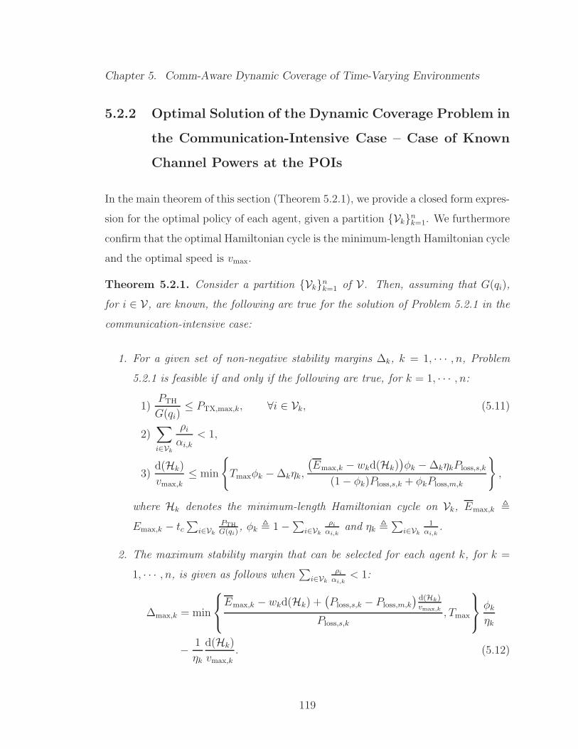
Chapter 5. Comm-Aware Dynamic Coverage of Time-Varying Environments
5.2.2 Optimal Solution of the Dynamic Coverage Problem in
the Communication-Intensive Case – Case of Known
Channel Powers at the POIs
In the main theorem of this section (Theorem 5.2.1), we provide a closed form expres-
sion for the optimal policy of each agent, given a partition Vknk=1. We furthermore
confirm that the optimal Hamiltonian cycle is the minimum-length Hamiltonian cycle
and the optimal speed is vmax.
Theorem 5.2.1. Consider a partition Vknk=1 of V. Then, assuming that G(qi),
for i ∈ V, are known, the following are true for the solution of Problem 5.2.1 in the
communication-intensive case:
1. For a given set of non-negative stability margins ∆k, k = 1, · · · , n, Problem5.2.1 is feasible if and only if the following are true, for k = 1, · · · , n:
1)PTH
G(qi)≤ PTX,max,k, ∀i ∈ Vk, (5.11)
2)∑
i∈Vk
ρiαi,k
< 1,
3)d(Hk)
vmax,k≤ min
Tmaxφk −∆kηk,
(Emax,k − wkd(Hk)
)φk −∆kηkPloss,s,k
(1− φk)Ploss,s,k + φkPloss,m,k
,
where Hk denotes the minimum-length Hamiltonian cycle on Vk, Emax,k ,
Emax,k − tc∑
i∈Vk
PTH
G(qi), φk , 1−∑i∈Vk
ρiαi,k
and ηk ,∑
i∈Vk
1αi,k
.
2. The maximum stability margin that can be selected for each agent k, for k =
1, · · · , n, is given as follows when∑
i∈Vk
ρiαi,k
< 1:
∆max,k = min
Emax,k − wkd(Hk) +
(Ploss,s,k − Ploss,m,k
) d(Hk)vmax,k
Ploss,s,k
, Tmax
φk
ηk
− 1
ηk
d(Hk)
vmax,k. (5.12)
119

Chapter 5. Comm-Aware Dynamic Coverage of Time-Varying Environments
3. There exists a feasible stabilizing policy, i.e., Problem 5.2.1 is feasible for at
least one set of non-negative ∆k, if and only if the following are true, for
k = 1, · · · , n:
1)PTH
G(qi)≤ PTX,max,k, ∀i ∈ Vk, (5.13)
2)∑
i∈Vk
ρiαi,k
< 1,
3)d(Hk)
vmax,k
≤ min
Tmax,
Emax,k − wkd(Hk)
(1− φk)Ploss,s,k + φkPloss,m,k
φk.
4. If Problem 5.2.1 is feasible, the optimal Hamiltonian cycle, velocity and trans-
mission power of the kth agent, for k = 1, · · · , n, are given as follows: C∗k = Hk,
v∗k = vmax,k and P ∗TX,i,k = PTH
G(qi), for all i ∈ Vk. We also have the following for
the optimal stop times and total energy of the mobile agents:
1) t∗i,k = ∆k
(1
αi,k+
ρiηkαi,kφk
)+
ρiαi,kφk
d(Hk)
vmax,k, ∀i ∈ Vk, (5.14)
2) E∗k = Ploss,s,k
(∆kηkφk
+1− φk
φk
d(Hk)
vmax,k
)+
(Ploss,m,k
vmax,k+ wk
)d(Hk)
+ tc∑
i∈Vk
PTH
G(qi).
Proof. Consider (5.60) where a partition Vknk=1 is given. In this case, the problem
becomes decoupled and can be solved individually for each mobile agent. It can
be immediately seen that the optimal TX power for each mobile agent k is the
minimum possible transmission power required to make the POIs in Vk connected,
i.e., P ∗TX,i,k = PTH
G(qi), for i ∈ Vk. Thus, the first set of conditions for feasibility of the
problem are PTH
G(qi)≤ PTX,max,k, for i ∈ Vk and k = 1, · · · , n. Moreover, for any set of
stop times ti,k, for i ∈ Vk, the total energy and the period are increasing functions of
d(Ck) and decreasing functions of vk. Thus, to obtain the minimum total energy, the
optimal cycle is the one with the minimum total length, i.e., the minimum-length
Hamiltonian cycle Hk, and the optimal velocity is the maximum possible velocity,
i.e., vmax,k.
120

Chapter 5. Comm-Aware Dynamic Coverage of Time-Varying Environments
Let us replace d(Ck) with d(Hk) and vk with vmax,k in (5.60). Also, let us define
Emax,k , Emax,k − tc∑
i∈Vk
PTH
G(qi). Then, the optimal stop times for each mobile agent
k are given by the solution of the following optimization problem, provided that the
optimal stop times are all positive:
min∑
i∈Vkti,k,
s.t.
1) αi,kti,k − ρi
(∑j∈Vk
tj,k +d(Hk)vmax,k
)≥ ∆k, ∀i ∈ Vk,
2)∑
i∈Vkti,k +
d(Hk)vmax,k
≤ Tmax,
3) Ploss,s,k
∑i∈Vk
ti,k +(
Ploss,m,k
vmax,k+ wk
)d(Hk) ≤ Emax,k.
(5.15)
This optimal solution of this linear program satisfies the Karush-Kuhn-Tucker (KKT)
conditions. The Lagrangian of the problem is given by
Lk =∑
i∈Vk
ti,k −∑
i∈Vk
µi,k
(αi,kti,k − ρi
∑
j∈Vk
tj,k − ρid(Hk)
vmax,k
−∆k
)+ (5.16)
γk
(∑
i∈Vk
ti,k +d(Hk)
vmax,k− Tmax
)+ νk
(Ploss,s,k
∑
i∈Vk
ti,k +Ploss,m,kd(Hk)
vmax,k+ wkd(Hk)− Emax,k
),
where µi,k, γk and νk are the Lagrange multipliers. The KKT conditions are then as
follows:
1) ∂Lk
∂ti,k= 1− αi,kµi,k +
∑j∈Vk
µj,kρj + γk + νkPloss,s,k = 0, ∀i ∈ Vk,
2) µi,k
(αi,kti,k − ρi
∑j∈Vk
tj,k − ρid(Hk)vmax,k
−∆k
)= 0, ∀i ∈ Vk,
3) γk
(∑i∈Vk
ti,k +d(Hk)vmax,k
− Tmax
)= 0,
4) νk
(Ploss,s,k
∑i∈Vk
ti,k +Ploss,m,kd(Hk)
vmax,k+ wkd(Hk)− Emax,k
)= 0,
5) αi,kti,k − ρi∑
j∈Vktj,k − ρi
d(Hk)vmax,k
−∆k ≥ 0,
6)∑
i∈Vkti,k +
d(Hk)vmax,k
− Tmax ≤ 0,
7) Ploss,s,k
∑i∈Vk
ti,k +Ploss,m,kd(Hk)
vmax,k+ wkd(Hk)−Emax,k ≤ 0,
8) µi,k ≥ 0, ∀i ∈ Vk, γk ≥ 0, νk ≥ 0.
(5.17)
From the first set of conditions in (5.17), we conclude that µi,k > 0, for i ∈ Vk, which
results in the following optimality conditions: αi,kti,k − ρi∑
j∈Vktj,k − ρi
d(Hk)vmax,k
= ∆k,
121

Chapter 5. Comm-Aware Dynamic Coverage of Time-Varying Environments
for i ∈ Vk. By solving this set of equations, we get the following for the optimal stop
times:
t∗i,k = ∆k
(1
αi,k
+ρiηkαi,kφk
)+
ρiαi,kφk
d(Hk)
vmax,k
, ∀i ∈ Vk, (5.18)
∑
i∈Vk
t∗i,k = ∆kηkφk
+d(Hk)
vmax,k
1− φk
φk,
where φk , 1−∑i∈Vk
ρiαi,k
and ηk ,∑
i∈Vk
1αi,k
. It can be seen that the optimal stop
times are all positive when∑
i∈Vk
ρiαi,k
< 1, for k = 1, · · · , n, which form the second
set of conditions for the feasibility of the optimization problem. The third set of such
conditions are also given as follows:
Ploss,s,k
(∆k
ηkφk
+d(Hk)
vmax,k
1− φk
φk
)+
(Ploss,m,k
vmax,k
+ wk
)d(Hk) ≤ Emax,k,
∆kηkφk
+d(Hk)
vmax,k
1
φk≤ Tmax,k. (5.19)
After combining these two constraints, we then obtain the third set of feasibility
conditions in part 1 of Theorem 5.2.1. The maximum stability margin is also the
maximum ∆k that satisfies (5.19), which can be shown to be the same as ∆max,k in
part 2 of Theorem 5.2.1. Finally, by setting ∆k = 0 in (5.19), we get the conditions
of (5.13) in part 3 of Theorem 5.2.1.
Theorem 5.2.1 can be used to determine whether there exists a feasible stabilizing
policy for a given partition Vknk=1. Then, we can find the optimal solution to
Problem 5.2.1 by searching through all the partitions Vknk=1 of V that satisfy (5.11),
and finding the one with minimum∑n
k=1kE∗k . A more efficient alternative for
solving Problem 5.2.1 is to use a mixed-integer program (MIP) to find the optimal
partitions and optimal stopping times for the mobile agents, when the maximum
allowed velocities and minimum possible transmission powers are used. Generally,
there is more than one way to formulate the MIP. Since there are multiple mobile
agents, some MIP formulations can be nonlinear, in which case the optimal solution
122

Chapter 5. Comm-Aware Dynamic Coverage of Time-Varying Environments
is very challenging to find. Next, we show how to formulate a mixed-integer linear
program (MILP), by transforming the nonlinear mixed-integer constraints to linear
ones. This makes finding the optimal dynamic coverage policies tractable even for
large number of POIs. Note that MILPs can be solved much more efficiently than
their nonlinear alternatives. There exists several solvers, such as IBM ILOG CPLEX
[104] and SAS/OR [105], that can solve large-scale MILP considerably fast.
Let us consider auxiliary binary variables xi,k and zi,j,k, for i, j ∈ V and k =
1, · · · , n. We have xi,k = 1 whenever the ith POI is assigned to the kth mobile
agent, and xi,k = 0 otherwise. Also, zi,j,k = 1 if there exists an edge between
the ith and jth POIs in the Hamiltonian cycle assigned to the kth mobile agent,
and zi,j,k = 0 otherwise. To guarantee that every POI that is on the Hamiltonian
cycle Vk have one degree in and one degree out, we can add the following set of
constraints:∑m
j=1,j 6=i zi,j,k = xi,k,∑m
j=1,j 6=i zj,i,k = xi,k, for all i ∈ V. Then, by
defining di,j , ‖qi − qj‖, we have the following constraints for the period and total
energy per period of the kth agent:
m∑
i=1
xi,kti,k +1
vmax,k
m∑
i=1
m∑
j=1,j 6=i
zi,j,kdi,j ≤ Tmax, (5.20)
Ploss,s,k
m∑
i=1
xi,kti,k +
(Ploss,m,k
vmax,k
+ wk
) m∑
i=1
m∑
j=1,j 6=i
zi,j,kdi,j + tc
m∑
i=1
xi,kPTH
G(qi)≤ Emax,k,
with ti,k ≥ 0 for all i, k. As can be seen, the left-hand side of both constraints
are nonlinear functions of ti,k and xi,k. In order to make the constraints linear, we
consider a large constant Ω > 0. We then add the linear constraints ti,k ≤ xi,kΩ,
for all i, k, to guarantee that ti,k = 0 whenever xi,k = 0 (i 6∈ Vk), while there is no
constraint on ti,k whenever xi,k = 1 (i ∈ Vk). This way we can replace the nonlinear
term xi,kti,k with ti,k in (5.20), without changing the optimal solution. Furthermore,
since the kth mobile agent does not need to stabilize any POI out of Vk, we should
modify the stability constraints of the kth mobile agent such that they automatically
become true for all i 6∈ Vk. This is done by considering the following stability
123

Chapter 5. Comm-Aware Dynamic Coverage of Time-Varying Environments
constraints:
αi,kti,k − ρi
(m∑
i=1
ti,k +1
vmax,k
m∑
i=1
m∑
j=1,j 6=i
zi,j,kdi,j
)+ (1− xi,k)Ω ≥ ∆k, ∀i, k. (5.21)
We can see that when xi,k = 0, constraint (5.21) becomes true if Ω > 0 is large
enough. It is easy to confirm that any Ω ≥ maxTmax,
(maxi ρi
)Tmax + maxk ∆k
can be considered large enough for this set of constraints. Such an Ω also guarantees
that whenever xi,k = 1, the constraint ti,k ≤ xi,kΩ is always true. Based on this
discussion, the MILP formulation for solving Problem 5.2.1 is given by Program 1.
Program 1 MILP for solving Problem 5.2.1 in the communication-intensive case
min∑n
k=1kEk,
s.t.
1) αi,kti,k − ρi
(∑mi=1 ti,k +
1vmax,k
∑mi=1
∑mj=1,j 6=i zi,j,kdi,j
)+ (1− xi,k)Ω ≥ ∆k, ∀i, k,
2)∑m
i=1 ti,k +1
vmax,k
∑mi=1
∑mj=1,j 6=i zi,j,kdi,j ≤ Tmax, ∀k,
3) Ploss,s,k
∑mi=1 ti,k +
(Ploss,m,k
vmax,k+ wk
)∑mi=1
∑mj=1,j 6=i zi,j,kdi,j + tc
∑mi=1
xi,kPTH
G(qi)≤ Ek, ∀k,
4)∑m
j=1,j 6=i zi,j,k = xi,k,∑m
j=1,j 6=i zj,i,k = xi,k, ∀i, k,
5)∑n
k=1 xi,k = 1, ∀i,
6)∑m
i=1 hi = n,
7) ui − uj −m(hi + hj) + (m− 1)∑n
k=1 zi,j,k ≤ m− 2, ∀i, j 6= i,
8) 2− hi ≤ ui ≤ m, ∀i,9) ti,k ≤ xi,kΩ, ∀i, k,10) xi,k
PTH
G(qi)≤ PTX,max,k, ∀i, k,
11) Ek ≤ Emax,k, ∀k,12) zi,j,k ∈ 0, 1, xi,k ∈ 0, 1, hi ∈ 0, 1, ui ∈ N, 0 ≤ ti,k ≤ Ω, ∀i, j, k,
Constraints 1, 2 and 3 in Program 1 are the stability, time and energy constraints,
as introduced before. Constraint 4 forces each POI i ∈ V to have exactly one degree in
124

Chapter 5. Comm-Aware Dynamic Coverage of Time-Varying Environments
and one degree out. Constraint 5 guarantees that each POI is assigned to one mobile
agent.5 Constraints 6, 7 and 8 are the sub-tour elimination constraints (SECs),
which are added to prevent any invalid sub-tour on the set of POIs assigned to
each agent [106]. To prevent sub-tours, we have introduced 2m auxiliary variables
hi and ui, for i ∈ V, and used a modified version of the well-known Miller-Tucker-
Zemlin (MTZ) constraints [106, 107]. Constraint 9 forces ti,k = 0 whenever xi,k = 0.
Constraint 10 is the transmission power constraint, which implies that if a POI is
assigned to a mobile agent, that mobile agent should be able to be connected at the
position of the POI. Finally, constraint 11 is the constraint on the maximum total
energy consumption in each period.
It is worth mentioning that MTZ formulations for sub-tour elimination, as used
in vehicle routing problem (VRP) or multiple traveling salesman problem (mTSP),
typically assume a fixed POI, called depot, through which all the mobile agents must
pass [108]. The MTZ formulation used in Program 1 is different from those formu-
lations, as it assumes no depot [107]. The idea here is to introduce floating depot
variables hi, for i ∈ V, which guarantee that whenever hi = 1 (the ith POI is selected
as a depot), constraint 7 in Program 1 is always true. Also note that, in general, the
MTZ formulation has a polynomial size (i.e., the number of SECs is of polynomial
order), compared to the exponential size of several alternative formulations in the
literature [108].
For n mobile agents and m POIs, the MILP of Program 1 has nm(m+1)+2m+n
variables (nm2 +m binaries, nm + n reals and n integers), 3nm +m(m + 1) + 2n
inequality constraints and 2nm+m+1 equality constraints. This MILP can be solved
using several efficient solvers, such as IBM ILOG CPLEX [104] and SAS/OR [105].
5Note that if xi,k = 1, the kth mobile agent needs to visit at least one more POI (otherthan POI i) to satisfy constrain 4 in Program 1. Therefore, the case of one single POIassigned to one agent is automatically prevented, i.e., |Vk| > 1 for all k.
125

Chapter 5. Comm-Aware Dynamic Coverage of Time-Varying Environments
Fig. 5.2 shows a sample plot of Ψi(t) for one of the POIs after optimizing the
dynamic coverage operation using the proposed MILP. Fig. 5.2 (left) corresponds to
the case where ∆k > 0 (robust dynamic coverage with positive stability margin) and
Fig. 5.2 (right) corresponds to the case where ∆k = 0 (zero stability margin). It can
be seen that a positive stability margin results in a longer stop time and, as a direct
result, more energy consumption at the point of interest, as proved by Theorem 5.2.1.
0 5 10 15 20 25 300
2
4
6
8
10
t (s)
Ψi(t)
0 5 10 15 20 25 300
2
4
6
8
10
t (s)
Ψi(t)
Figure 5.2: A sample plot of Ψi(t) at the remote station in the communication-intensivecase, for one of the POIs, after optimizing the dynamic coverage operation using the MILPof Program 1. The left figure corresponds to the case where ∆k > 0 (robust dynamiccoverage with positive stability margin) and the right one corresponds to the case where∆k = 0 (zero stability margin).
5.2.3 Optimal Solution of the Dynamic Coverage Problem in
the Communication-Intensive Case – Case of Unknown
Stochastic Channel Powers at the POIs
So far, we have assumed that the channel powers G(qi), for i ∈ V, are known before-
hand when solving Problem 5.2.1. This, however, may not be the case in practical
applications, where the channel power may only be known at a small number of
126

Chapter 5. Comm-Aware Dynamic Coverage of Time-Varying Environments
positions in the workspace that are different from the positions of the POIs. For
such cases, we can use the probabilistic channel prediction framework of Chapter 2
to assess the channel powers at the positions of the POIs. Stochastic channel powers,
however, result in stochastic constraints in Problem 5.2.1. It is then desired to find al-
ternative deterministic conditions that guarantee that the feasibility conditions hold
with a probability larger than a given threshold. This is, however, very challenging
in general, due to the fact that the conditions are complex functions of the stochastic
channel powers. To simplify the problem in the case of stochastic channel powers, we
propose using concepts from stochastic programming [109]. Stochastic programming
provides a systematic sub-optimal approach to transform the stochastic constraints
of an optimization problem to deterministic ones.
Several methods have been proposed in the stochastic programming literature
for this purpose, such as the expectation constraint method, worse-case constraint
method and chance constraint method [109]. In this section, we use the chance
constraint method, as it provides more robustness to stochasticity of the channel
and is yet easy to apply to our dynamic coverage problem. The idea behind the
chance constraint method is to replace any constraint that is directly a function of
the main random variables (G(qi) in our case) with its chance constrain. A chance
constraint is simply a constraint that guarantees that the probability of meeting the
stochastic constraint is larger than a given χ, for 0.5 < χ < 1, while assuming that
all the other optimization variables are deterministic [109]. Next, we show how to
solve the chance-constrained version of Problem 5.2.1, i.e., Problem 5.2.1, with its
stochastic constraints replaced with the corresponding chance constraints. In this
chapter, a feasible solution to this problem is called a χ-probable feasible stabilizing
dynamic coverage policy and is defined as follows:
Definition 5.2.4. The dynamic coverage policy P is called a χ-probable feasible
stabilizing dynamic coverage policy in the communication-intensive case if for this
127

Chapter 5. Comm-Aware Dynamic Coverage of Time-Varying Environments
policy the probability of meeting any stochastic constraint in Problem 5.2.1 is larger
than χ, for 0.5 < χ < 1.
Let us start by calculating the probability of meeting the stochastic constraint in
the chance-constrained version of Problem 5.2.1. Instead of deterministic G(qi), for
i ∈ V, we have the corresponding predicted channel GdB(qi) in dB (see Chapter 2).
Then, the minimum transmission power constraint (constraint 4 of Problem 5.2.1)
will have the following chance-constrained form:
P
PTX,i,k ≥
PTH
G(qi)
≥ χ, i ∈ Vk, k = 1, · · · , n. (5.22)
Similar to the previous chapters, in order to calculate PPTX,i,k ≥ PTH
G(qi)
, we use the
probabilistic channel assessment framework of Chapter 2. We then have
P
PTX,i,k ≥
PTH
G(qi)
= Q
(10 log10
(PTH
PTX,i,k
)− GdB(qi)
σ(qi)
), (5.23)
where Q(x) = 1√2π
∫∞xe−x2/2dx is the tail probability of a Gaussian distribution.
Note that we have dropped the dependency of channel assessment on k and t in
this case, as the channel is assessed beforehand, using a number of a priori channel
measurements, and used for finding the optimal dynamic coverage policy for all the
mobile agents. After some straightforward calculations, we can find the necessary
and sufficient condition for (5.22) as follows:
PTX,i,k ≥ 10−(σ(qi)Q−1(χ)+GdB(qi))/10 PTH , Γ(qi, χ), i ∈ Vk, k = 1, · · · , n, (5.24)
with Q−1(x) denoting the inverse of Q(x) (not to be confused with exponentiation).
This shows that in order to account for stochastic channels when designing optimal
dynamic coverage policies, it is sufficient to replace PTH
G(qi)with Γ(qi, χ) in Problem
5.2.1. After this modification, the MILP of Program 1 is readily applicable to this
case as well. Similarly, the results of Theorem 5.2.1 also hold. For instance, we can
128

Chapter 5. Comm-Aware Dynamic Coverage of Time-Varying Environments
show that, given the partition Vknk=1, there exists a χ-probable feasible stabilizing
policy for the kth agent, for k = 1, · · · , n, if and only if
1) Γ(qi, χ) ≤ PTX,max,k, ∀i ∈ Vk, (5.25)
2)∑
i∈Vk
ρiαi,k
< 1,
3)d(Hk)
vmax,k≤ min
Tmax,
Emax,k − tc∑
i∈ViΓ(qi, χ)− wkd(Hk)
(1− φk)Ploss,s,k + φkPloss,m,k
φk.
It is worth mentioning that, from (5.24), the average minimum transmit power re-
quired, to meet the constraint on the transmission power with a probability larger
than χ, for 0.5 < χ < 1, increases as the uncertainty in channel assessment (σ(qi))
gets larger. Finally, in a realistic communication scenario, results of both cases of
known and unknown channel powers can be useful. Since the dynamic coverage task
is periodic, the results for the unknown probabilistic case can first be used for plan-
ning. Then, once the agents measure the channel at their corresponding POIs, they
can share their channel measurements and solve the optimization problem for the
case of known channels.
5.2.4 Probabilistic Analysis of the Dynamic Coverage Prob-
lem in the Communication-Intensive Case
By probabilistic analysis of the dynamic coverage problem, we mean deriving condi-
tions for a policy P to be a χ-probable feasible stabilizing dynamic coverage policy
in case both the channel and the positions of the POIs are stochastic. Such analysis
provides a priori knowledge about the coverage task before the deployment of the
mobile agents, which is extremely useful for high-level planning purposes. It charac-
terizes the probability of having a feasible stabilizing dynamic coverage policy, when
the channel power and the positions of the POIs are drawn from a certain distribu-
tion. Without loss of generality, we consider the following extra assumptions in this
129

Chapter 5. Comm-Aware Dynamic Coverage of Time-Varying Environments
section for the ease of mathematical derivations:6
Assumption 5.2.1. The rate of increasing Ψi(t) and the service rate of each agent
k are identical at all the POIs, i.e., ρi = ρ and αi,k = αk, for i ∈ V and k = 1, · · · , n.
Assumption 5.2.2. The motion power loss, while a mobile agent is moving, is equal
to its motion power loss when it stops at a POI, i.e., Ploss,s,k = Ploss,m,k = Ploss,k, for
k = 1, · · · , n.
Assumption 5.2.3. The POIs assigned to the kth mobile agent, for k = 1, · · · , n,are independently and identically distributed (i.i.d.) according to an absolutely con-
tinuous pdf ψ(q) which is defined over the workspace W. Furthermore, the number
of these POIs is large.7
In order to better follow the discussion, it would be easier to assume the case of
known channels, i.e., for any realization of the channel, the agents plan based on the
full knowledge of the channel.
As explained in Section 5.2.3, in case of stochastic constraints in Problem 5.2.1,
the optimal strategy is to directly calculate the probability of having a feasible stabi-
lizing dynamic coverage policy and derive conditions that guarantee this probability
is larger than a threshold. If both the channel powers at the POIs and their positions
are stochastic, however, deriving such conditions is extremely challenging. There-
fore, similar to Section 5.2.3, we use a sub-optimal approach based on stochastic
programming, i.e., we treat the rest of the variables, aside from channel power and
the positions of the POIs, deterministically.
6Note that these assumptions are made to simplify the theoretical analysis of this sec-tion. Similar results can be found for the case that either one of these assumptions doesnot hold. For instance, the results of this section can be easily extended to the case that ρi,for i = 1, · · · , n, are i.i.d. random variables, independent of the channel and the positionsof the POIs, or to the case where Ploss,s,k 6= Ploss,m,k.
7The meaning of a large number of POIs will be explained later in this section.
130

Chapter 5. Comm-Aware Dynamic Coverage of Time-Varying Environments
Let mk = |Vk| represent the number of POIs assigned to the kth mobile agent. We
calculate the probabilities of meeting the stochastic constraints by first conditioning
on the positions of the POIs and then averaging over their probability distributions.
Using the results of the previous section, we conclude that in the case of randomly
positioned POIs, we have
P
PTX,i,k ≥
PTH
G(qi)
=
∫
WQ
10 log10
(PTH
PTX,i,k
)− GdB(q)
σ(q)
ψ(q)dq ≥ χ, (5.26)
where GdB(q) and σ2(q) are the mean and variance of a Gaussian distribution that
characterizes the channel power (in the dB domain) at a position q ∈ W. Since the
left-hand side of (5.26) is an increasing function of PTX,i,k, we have the following for
all the POIs assigned to the kth agent:
PTX,i,k ≥ 10−GdB(χ)/10 PTH , Γ(χ), i ∈ Vk, k = 1, · · · , n, (5.27)
where GdB(χ) is the unique solution to the following equation as a function of G:
∫
WQ
(G− GdB(q)
σ(q)
)ψ(q)dq = χ. (5.28)
Next, consider all the constraints of Problem 5.2.1 that are functions of the d(Ck).Based on the previous results, the optimum Hamiltonian cycles are the minimum-
length Hamiltonian cycles. Therefore, we can find the probability of meeting the
constraints as a function of d(Hk) instead, where Hk is the minimum-length Hamil-
tonian cycle on Vk. Since the constraints of Problem 5.2.1 are linear with respect
to d(Hk), we are then required to find the probabilities of the form P d(Hk) ≤ c,for a constant c. Such probabilities can be found using the following result from the
probabilistic traveling salesman problem (TSP) literature [106]:
Lemma 5.2.2. Assume that the spatial distribution of POIs is i.i.d., according to an
absolutely continuous pdf ψ(q) defined over the compact set W. Then, there exists a
131

Chapter 5. Comm-Aware Dynamic Coverage of Time-Varying Environments
constant θTSP such that
1) P
lim
mk→∞
d(Hk)√mk
= θTSP
∫
W
√ψ(q)dq
= 1,
2) limmk→∞
Ed(Hk)
√mk
= θTSP
∫
W
√ψ(q)dq, (5.29)
where mk = |Vk| is the number of POIs assigned to the kth mobile agent.
Proof. See [106].
The constant θTSP is estimated to be around 0.765 [110]. Let us define ζ ,
θTSP
∫W√ψ(q)dq. By using Lemma 5.2.2 and by considering the constraint (5.27)
on the transmission power of each mobile agent, we conclude that, for large mk, the
results of Theorem 5.2.1 hold in this case too, provided that d(Hk) is replaced by
ζ√mk,
PTH
G(qi)is replaced by Γ(χ), and mk remains large.8 Therefore, given a partition
Vknk=1, there exists a χ-probable feasible stabilizing dynamic coverage policy, i.e.,
the chance-constrained version of Problem 5.2.1 is feasible, if and only if the following
are true, for k = 1, · · · , n:
1) Γ(χ) ≤ PTX,max,k, (5.30)
2) mk <αk
ρ,
3) min
Emax,k − tcmkΓ(χ)− wkζ
√mk
Ploss,k
, Tmax
(1−mk
ρ
αk
)≥ ζ
√mk
vmax,k
.
Note that for (5.30) to be a precise condition, mk is required to be large. That is
why the second part of Assumption 5.2.3 is necessary for the analysis of this section.
For convex environments, mk ≥ 15 can be assumed sufficiently large. In other words,
for mk ≥ 15, ζ√mk is a tight approximation for the length of the minimum-length
Hamiltonian cycle on the set of POIs assigned to the kth agent [110]. On the other
hand, the set of constraints in (5.30) may not be feasible for very large mk. In
8Note that no MILP needs to the be solved in this case.
132

Chapter 5. Comm-Aware Dynamic Coverage of Time-Varying Environments
fact, there is an upper-bound on the maximum number of access points that can be
assigned to each agent, as we characterize next.
An Upper Bound on the Maximum Number of POIs Covered by a Mobile
Agent in the Communication-Intensive Case
Consider the following theorem:
Theorem 5.2.2. Assume that for the kth agent and for the given χ, we have Γ(χ) ≤PTX,max,k, where Γ(χ) is given by (5.27). Then, under Assumptions 5.2.1, 5.2.2 and
5.2.3, an upper-bound on the maximum number of POIs that can be assigned to the
kth agent, to guarantee a χ-probable feasible stabilizing dynamic coverage policy in
the communication-intensive case, is given as follows:
mk =
mins2k,1, s
2k,2
, Ak ∩ Bk = ∅, Emax,k > Ploss,kTmax
maxs2∣∣s ∈ Ak ∩ Bk
, Ak ∩ Bk 6= ∅, Emax,k > Ploss,kTmax
maxs2∣∣s ∈ A′
k ∩ Bk
, A′
k ∩ Bk 6= ∅, Emax,k ≤ Ploss,kTmax
, (5.31)
provided that such mk exists (chance-constrained version of Problem 5.2.1 is feasible)
and it is sufficiently large. Here,
sk,1 =−ζ/vmax,k +
√ζ2/v2max,k + 4T 2
maxρ/αk
2Tmaxρ/αk, (5.32)
sk,2 =−ζwk +
√ζ2w2
k + 4tcΓ(χ) (Emax,k − Ploss,kTmax)
2tcΓ(χ),
sk,3 = min
√αk
ρ,−ζwk +
√ζ2w2
k + 4tcΓ(χ)Emax,k
2tcΓ(χ)
,
Ak =s∣∣sk,2 ≤ s ≤ sk,3
, A′
k =s∣∣0 ≤ s ≤ sk,3
,
Bk =
s
∣∣∣∣(ζPloss,k
vmax,k+ ζwk
)s+
(tcΓ(χ) +
Emax,kρ
αk
)s2− ζwkρ
αks3 − tcΓ(χ)ρ
αks4 ≤ Emax,k
.
Proof. Consider the constraints in (5.30) and assume that mk is large enough. By
defining the variable s ,√mk and after some straightforward derivations, we can
133

Chapter 5. Comm-Aware Dynamic Coverage of Time-Varying Environments
conclude that any feasible s ≥ 0 satisfies one of the following sets of constraints:
1) Tmaxραk
s2 + ζvmax,k
s ≤ Tmax, tcΓ(χ)s2 + wkζs ≤ Emax,k − Ploss,kTmax, or 2) Emax,k ≥
tcΓ(χ)s2 + wkζs ≥ Emax,k − Ploss,kTmax,
(ζPloss,k
vmax,k+ ζwk
)s +
(tcΓ(χ) +
Emax,kρ
αk
)s2 −
ζwkραk
s3 − tcΓ(χ)ραk
s4 ≤ Emax,k, s2 ≤ αk
ρ. First assume that Emax,k > Ploss,kTmax. Then,
the maximum s ≥ 0 that satisfies the first set of constraints is simply the minimum
of the positive roots of Tmaxραk
s2 + ζvmax,k
s = Tmax and tcΓ(χ)s2 + wkζs = Emax,k −
Ploss,kTmax, which are sk,1 and sk,2 in (5.32), respectively. Similarly, any s ≥ 0
that satisfies the second set of constraints 1) must be greater than or equal to sk,2
and less than or equal to the minimum of√
αk
ρand the positive root of tcΓ(χ)s
2 +
wkζs = Emax,k, which is sk,3 in (5.32), and 2) must satisfy the fourth-order polynomial
inequality in the second set of constraints. Therefore, the maximum s that satisfies
the second set of constraints is simply the maximum s in Ak ∩ Bk, for Ak and Bk
defined in (5.32). Note that all the elements of Ak ∩ Bk are necessarily greater than
or equal to minsk,1, sk,2
. Therefore, if Ak ∩ Bk 6= ∅, the upper bound on s is the
maximum element of Ak ∩ Bk. However, if Ak ∩ Bk = ∅, the upper bound on s is
given by minsk,1, sk,2
.
Next, assume that Emax,k ≤ Ploss,kTmax. In this case the first set of constraints
does not hold for any s ≥ 0 and only the second set of constraints needs to be con-
sidered. Following a similar procedure, we can conclude that the maximum possible
s that satisfies the second set of constraints is the maximum s in A′k ∩ Bk. This
completes the proof.
Average Minimum Energy Per Period Consumed to Cover a Set of POIs
by a Mobile Agent in the Communication-Intensive Case
Another interesting quantity to characterize probabilistically is the average of the
minimum energy consumed in one period by the kth mobile agent to feasibly stabilize
its assigned POIs. This is given by the following theorem in case of large mk:
134

Chapter 5. Comm-Aware Dynamic Coverage of Time-Varying Environments
Theorem 5.2.3. Consider Assumptions 5.2.1, 5.2.2 and 5.2.3. Then, the average
of the minimum energy consumed in one period by the kth mobile agent to feasibly
stabilize its assigned POIs is given as follows in the communication-intensive case:
Emin,ave,k =
Ploss,k(1−mk
ραk
)vmax,k
+ wk
ζ√mk + tcmkPTH
∫
W
exp(12σ2(q)
)
10GdB(q)
10
ψ(q)dq,
(5.33)
where GdB(q) and σ2(q) are the mean and variance of a Gaussian distribution that
characterizes the channel power at a position q ∈ W in the dB domain, σ(q) ,log(10)
10σ(q), mk <
αk
ρ, and mk remains large enough.
Proof. The minimum energy occurs when the stability margin is zero. By setting
∆k = 0 in (5.14), and based on Assumptions 5.2.1, 5.2.2 and 5.2.3, we obtain
Emin,ave,k = E E∗k =
Ploss,k(
1−mkραk
)vmax,k
+ wk
Ed(Hk)
+ tcmkPTH
∫
WE
1
G(q)
∣∣∣∣qψ(q)dq, (5.34)
where averaging is done over every possible distribution of the channel. The channel
power G(q) is log-normally distributed in linear domain (Gaussian distributed, with
mean GdB(q) and variance σ2(q), in the dB domain). We have
E
1
G(q)
∣∣∣∣q
=
∫ ∞
0
10
log(10)√2πσ(q)G2
exp
(−(10 log10(G)− GdB(q)
)2
2σ2(q)
)dG
=exp
(12σ2(q)
)
10GdB(q)
10
. (5.35)
Also, using Lemma 5.2.2, Ed(Hk)
= ζ
√mk for large mk. After substituting
E
1
G(q)
∣∣∣qand E
d(Hk)
into (5.34), (5.33) is obtained.
Note that Theorem 5.2.3 characterizes the exact average minimum energy con-
sumption, as it directly calculates the average of E∗k in (5.14) over the distributions
of the channel and POIs.
135

Chapter 5. Comm-Aware Dynamic Coverage of Time-Varying Environments
5.3 Dynamic Coverage of Time-Varying Environ-
ments in the Communication-Efficient Case
In this section, we study dynamic coverage of time-varying environments in the
communication-efficient case. Unlike the communication-intensive case, the mobile
agents are not required to be connected at the positions of all POIs in this case, as
long as they are connected at least once along their trajectories. Next, we present
the definition of the dynamic coverage policy in the communication-efficient case
and formulate the problem. We then show how to design optimal feasible stabilizing
policies for the mobile agents in this case.
5.3.1 Problem Formulation
Consider the dynamical system of (5.2). Similar to the communication-intensive case,
a dynamic coverage policy in the communication-efficient case is defined as follows:
Definition 5.3.1. In the communication-efficient case, a dynamic coverage policy
for the kth mobile agent is a tuple Pk =(Vk, Ck, vk, ξTX,k, PTX,k, ti,ki∈Vk
), where
Vk is the non-empty set of POIs assigned to the kth agent, Ck is the Hamiltonian
cycle defined on Vk, vk is the constant velocity of the kth agent, ξTX,k is the only
position along the Hamiltonian cycle Ck assigned for communication, PTX,k is the
transmission power of the kth agent at ξTX,k, and ti,k, for i ∈ Vk, is the stop time of
the kth mobile agent at the ith POI. The overall dynamic coverage policy to find is
then the tuple P = (P1, · · · ,Pn).
Note that we have assumed only one transmission in one period.9 The definitions
9The results can be easily extended to the case of multiple transmissions in one period.Multiple transmission is, in particular, useful to increase the spatial diversity and thereforethe robustness of the proposed scheme to multipath fading and other channel assessmenterrors.
136

Chapter 5. Comm-Aware Dynamic Coverage of Time-Varying Environments
of the feasible coverage policies, stable coverage tasks, and the conditions for a policy
P to be a feasible stabilizing policy in the communication-efficient case are also
similar to the communication-intensive case. The only differences are as follows: 1)
the total communication energy tc∑
i∈VkPTX,i,k in the second condition of (5.8) is
replaced by tcPTX,k, 2) PTX,i,k in the third condition of (5.8) is replaced by PTX,k,
for all i ∈ Vk, and 3) the channel powers G(qi), in the third condition of (5.8),
are replaced by G(ξTX,k). Here, the communication-time tc is as defined in the
communication-intensive case.
In order to maximize the lifetime of the mobile agents, we therefore have the
following optimization problem to find the optimal feasible stabilizing policies in the
communication-efficient case:
Problem 5.3.1. The maximum-lifetime feasible stabilizing dynamic coverage policy
for coverage of time-varying environments in the communication-efficient case is
given as follows:
minP,E1,··· ,En
n∑
k=1
kEk, (5.36)
s.t.
1) αi,kti,k − ρi
(∑
i∈Vk
ti,k +d(Ck)vk
)≥ ∆k, ∀i ∈ Vk, k = 1, · · · , n,
2)∑
i∈Vk
ti,k +d(Ck)vk
≤ Tmax, k = 1, · · · , n,
3) Ploss,s,k
∑
i∈Vk
ti,k +
(Ploss,m,k
vk+ wk
)d(Ck) + tcPTX,k ≤ Ek, k = 1, · · · , n,
4) PTX,max,k ≥ PTX,k ≥PTH
G(ξTX,k), k = 1, · · · , n, (5.37)
5) 0 ≤ vk ≤ vmax,k, k = 1, · · · , n,
6) Ek ≤ Emax,k, k = 1, · · · , n,
where we set ∆k ≥ 0 and k > 0.
137

Chapter 5. Comm-Aware Dynamic Coverage of Time-Varying Environments
Note that in the communication-efficient case, the communication points ξTX,k,
for k = 1, · · · , n, also need to be optimized. Also, here the mobile agents do not stop
to communicate at the communication points, i.e., they transmit for a time interval
with length tc as they move.10 Next we show how this dynamic coverage problem
can be optimally solved using an MILP, similar to the communication-intensive case.
5.3.2 Optimal Solution of the Dynamic Coverage Problem
in the Communication-Efficient Case – Case of Known
Channel Powers at the POIs
Consider Problem 5.3.1. Based on the definition of the dynamic coverage policy in
the communication-efficient case, ξTX,k can be any point on the Hamiltonian cycle Ckof the kth agent. Finding the optimal coverage policy in this case is very challenging.
This is due to the fact that given the partition Vknk=1 and conditioned on the
channel power over the workspace, the optimal Hamiltonian cycle for an agent k
may be different from the minimum-length Hamiltonian cycle Hk. In other words,
since there is no requirement for transmission at the POIs, moving to a point out
of the minimum-length Hamiltonian cycle can possibly minimize the communication
energy and the resulting overall energy consumption. To simplify the problem, we
consider the following assumption in this section:
Assumption 5.3.1. The communication point ξTX,k is selected from the set of POIs
Vk, i.e., ξTX,k = qi, for some i ∈ Vk.
Based on this assumption and given a partition Vknk=1, the optimal policy in
the communication-efficient case is then given by the following theorem:
10As compared to the communication-intensive case, tc could be larger in thecommunication-efficient case, since more data is sent to the remote station in each trans-mission. Still, we assume that tc is small enough such that the movement of the kth mobileagent while communicating, i.e., vmax,ktc, is negligible for all k.
138

Chapter 5. Comm-Aware Dynamic Coverage of Time-Varying Environments
Theorem 5.3.1. Consider a partition Vknk=1 of V. Then, assuming that the chan-
nel powers G(qi), for i ∈ V, are known, the following are true for the solution of
Problem 5.3.1, in the communication-efficient case:
1. For a given set of non-negative stability margins ∆k, k = 1, · · · , n, Problem5.3.1 is feasible if and only if the following are true, for k = 1, · · · , n:
1)PTH
maxi∈VkG(qi)
≤ PTX,max,k, (5.38)
2)∑
i∈Vk
ρiαi,k
< 1,
3)d(Hk)
vmax,k≤ min
Tmaxφk −∆kηk,
(Emax,k − wkd(Hk)
)φk −∆kηkPloss,s,k
(1− φk)Ploss,s,k + φkPloss,m,k
,
where Hk denotes the minimum-length Hamiltonian cycle on Vk, Emax,k ,
Emax,k − tcPTH
maxi∈VkG(qi) , φk , 1−∑i∈Vk
ρiαi,k
and ηk ,∑
i∈Vk
1αi,k
.
2. The maximum stability margin that can be selected for each agent k, for k =
1, · · · , n, is given as follows when∑
i∈Vk
ρiαi,k
< 1:
∆max,k = min
Emax,k − wkd(Hk) +
(Ploss,s,k − Ploss,m,k
) d(Hk)vmax,k
Ploss,s,k, Tmax
φk
ηk
− 1
ηk
d(Hk)
vmax,k. (5.39)
3. There exists a feasible stabilizing policy, i.e., Problem 5.2.1 is feasible for at
least one set of non-negative ∆k, if and only if the following are true, for
k = 1, · · · , n:
1)PTH
maxi∈VkG(qi)
≤ PTX,max,k, (5.40)
2)∑
i∈Vk
ρiαi,k
< 1,
3)d(Hk)
vmax,k≤ min
Tmax,
Emax,k − wkd(Hk)
(1− φk)Ploss,s,k + φkPloss,m,k
φk.
139

Chapter 5. Comm-Aware Dynamic Coverage of Time-Varying Environments
4. If Problem 5.3.1 is feasible, the optimal Hamiltonian cycle, velocity, transmis-
sion power and transmission point of the kth agent, for k = 1, · · · , n, are given
as follows: C∗k = Hk, v
∗k = vmax,k, P
∗TX,k = PTH
maxi∈VkG(qi) and ξ∗TX,k = qi∗
k, where
i∗k = argmaxi∈VkG(qi). We also have the following for the optimal stop times
and total energy of the mobile agents:
1) t∗i,k = ∆k
(1
αi,k+
ρiηkαi,kφk
)+
ρiαi,kφk
d(Hk)
vmax,k, ∀i ∈ Vk, (5.41)
2) E∗k = Ploss,s,k
(∆kηkφk
+1− φk
φk
d(Hk)
vmax,k
)+
(Ploss,m,k
vmax,k+ wk
)d(Hk)
+ tcPTH
maxi∈VkG(qi)
.
Proof. The proof is similar to the proof of Theorem 5.2.1 and is omitted for brevity.
Similar to the communication-intensive case, we next propose an MILP to solve
Problem 5.3.1. This MILP can be used to find the optimal partitions, optimal
Hamiltonian cycles, optimal communication points and optimal stopping times for
the mobile agents when the maximum allowed velocities and minimum possible trans-
mission powers are used. However, the MILP formulation is more complicated in this
case, since the optimal transmission points and, therefore, the optimal transmission
powers of the mobile agent are not known beforehand. The MILP formulation for
solving Problem 5.3.1 is given in Program 2.
In Program 2, the constant Ω′ is selected large enough, similar to Ω in Program
1. Furthermore, in addition to the variables used in Program 1, we have introduced
mn auxiliary binary variables yi,k, for i ∈ V and k = 1, · · · , n. For each mobile
agent k, yi,k = 1 if the ith POI is selected as the communication point, and yi,k = 0
otherwise. Constraint 10 in Program 2 guarantees that only one POI in Vk is selected
as the communication point. Constraint 11 also forces yi,k = 0 whenever xi,k = 0.
Explanation of other constraints is similar to Program 1. Fig. 5.3 shows sample
140

Chapter 5. Comm-Aware Dynamic Coverage of Time-Varying Environments
Program 2: MILP for solving Problem 5.3.1 in the communication-efficient case
min∑n
k=1kEk,
s.t.
1) αi,kti,k − ρi
(∑mi=1 ti,k +
1vmax,k
∑mi=1
∑mj=1,j 6=i zi,j,kdi,j
)+ (1− xi,k)Ω
′ ≥ ∆k, ∀i, k,2)∑m
i=1 ti,k +1
vmax,k
∑mi=1
∑mj=1,j 6=i zi,j,kdi,j ≤ Tmax, ∀k,
3) Ploss,s,k
∑mi=1 ti,k +
(Ploss,m,k
vmax,k+ wk
)∑mi=1
∑mj=1,j 6=i zi,j,kdi,j + tc
∑mi=1
yi,kPTH
G(qi)≤ Ek, ∀k,
4)∑m
j=1,j 6=i zi,j,k = xi,k,∑m
j=1,j 6=i zj,i,k = xi,k, ∀i, k,
5)∑n
k=1 xi,k = 1, ∀i,
6)∑m
i=1 hi = n,
7) ui − uj −m(hi + hj) + (m− 1)∑n
k=1 zi,j,k ≤ m− 2, ∀i, j 6= i,
8) 2− hi ≤ ui ≤ m, ∀i,
9) ti,k ≤ xi,kΩ′, ∀i, k,
10)∑m
i=1 yi,k = 1, ∀k,
11) yi,k ≤ xi,kΩ′, ∀i, k,
12) yi,kPTH
G(qi)≤ PTX,max,k, ∀i, k,
13) Ek ≤ Emax,k, ∀k,14) zi,j,k ∈ 0, 1, xi,k ∈ 0, 1, yi,k ∈ 0, 1, hi ∈ 0, 1, ui ∈ N, 0 ≤ ti,k ≤ Ω′, ∀i, j, k,
plots of Ψi(t) and Φi(t) for one of the POIs after optimizing the dynamic coverage
operation using the MILP of Program 2. Fig. 5.3 (left) corresponds to the case where
∆k > 0 (robust dynamic coverage with positive stability margin) and Fig. 5.3 (right)
corresponds to the case where ∆k = 0 (zero stability margin). It can be seen that,
similar to the communication-intensive case, a positive stability margin results in
longer stop time and more energy consumption at the point of interest, as proved in
Theorem 5.3.1. It can also be seen how Ψi(t) at the remote station becomes equal to
Φi(t) any time the mobile agent communicates to the remote station (in this example
141

Chapter 5. Comm-Aware Dynamic Coverage of Time-Varying Environments
the communication point is located at another POI).
0 5 10 15 20 25 300
5
10
15
t (s)
Ψi(t)
Φi(t)
0 5 10 15 20 25 300
5
10
15
t (s)
Ψi(t)
Φi(t)
Figure 5.3: Sample plots of Ψi(t) and Φi(t) in the communication-efficient case for oneof the POIs after optimizing the dynamic coverage operation using the MILP of Program2. The left figure corresponds to the case where ∆k > 0 (robust dynamic coverage withpositive stability margin) and the right figure corresponds to the case where ∆k = 0 (zerostability margin).
Virtual POIs in the Communication-Efficient Case
The coverage task in the communication-efficient case can be feasibly stabilized if
at least one POI is connected along the Hamiltonian cycle of each mobile agent (as
opposed to all POIs in the communication-intensive case). In case there is no feasible
stabilizing dynamic coverage policy in the communication-efficient case, due to a poor
channel quality at the POIs, we may be able to feasibly stabilize the coverage task by
adding a number of virtual POIs. These are points close enough to the actual POIs,
which have a good channel quality. Adding virtual POIs does not guarantee the
existence of a feasible stabilizing coverage policy. It, however, increases the chance
of finding such a policy in case the channel quality is low at the positions of the
actual POIs.
142

Chapter 5. Comm-Aware Dynamic Coverage of Time-Varying Environments
5.3.3 Optimal Solution of the Dynamic Coverage Problem in
the Communication-Efficient Case – Case of Unknown
Stochastic Channel Powers at the POIs
The definitions of the chance constraints and χ-probable feasible stabilizing dynamic
coverage policies, presented in Section 5.2.3 for Problem 5.2.1, can also be applied
to Problem 5.3.1 as well. Similarly, the minimum transmission power constraint
(constraint 4 of Problem 5.3.1) will have the following chance-constrained form:
P
PTX,k ≥
PTH
G(ξTX,k)
≥ χ, k = 1, · · · , n. (5.42)
Using the distribution of the channel power in the dB domain given by our channel
assessment framework of Chapter 2, we can show that this condition is equivalent to
PTX,k ≥ 10−(σ(ξTX,k)Q−1(χ)+GdB(ξTX,k))/10 PTH , Γ(ξTX,k, χ), k = 1, · · · , n. (5.43)
Similar to the communication-intensive case, this result shows that in order to ac-
count for stochastic channels, when designing optimal dynamic coverage policies in
the communication-efficient case, it is sufficient to replace PTH
G(ξTX,k)with Γ(ξTX,k, χ)
in Problem 5.3.1. Then, the results of Theorem 5.3.1 and the MILP of Program
2 can readily be used in this case as well. We can see that, given the partition
Vknk=1, the optimum communication point ξ∗TX,k is given by ξ∗TX,k = qi∗k, where
i∗k = argmini∈VkΓ(qi, χ). Also, there is a χ-probable feasible stabilizing policy for the
kth agent, for k = 1, · · · , n, if and only if
1)mini∈Vk
Γ(qi, χ) ≤ PTX,max,k, (5.44)
2)∑
i∈Vk
ρiαi,k
< 1,
3)min
Emax,k − tc mini∈Vk
Γ(qi, χ)− wkd(Hk)
(1− φk)Ploss,s,k + φkPloss,m,k, Tmax
φk ≥
d(Hk)
vmax,k.
143

Chapter 5. Comm-Aware Dynamic Coverage of Time-Varying Environments
5.3.4 Probabilistic Analysis of the Dynamic Coverage Prob-
lem in the Communication-Efficient Case
The same approach we used in Section 5.2.4 can be followed to probabilistically
analyze the dynamic coverage problem in the communication-efficient case. Assume
that the POIs are independently and identically distributed (i.i.d.) according to an
absolutely continuous pdf ψ(q), defined over the workspace W. Also, assume that,
conditioned on every q ∈ W, the channel power G(q) is Gaussian-distributed in the
dB domain, with GdB(q) and σ2(q) representing its mean and variance respectively.
By following the same (sub-optimal) chance constraint approach of Section 5.2.4 and
by considering Assumptions 5.2.1, 5.2.2 and 5.2.3, we can show that, given a partition
Vknk=1, there exists a χ-probable feasible stabilizing dynamic coverage policy for
this case if the following are true, for all k = 1, · · · , n:
1) Γ(χ) ≤ PTX,max,k, (5.45)
2) mk <αk
ρ,
3) min
Emax,k − tcΓ(χ)− wkζ
√mk
Ploss,k, Tmax
(1−mk
ρ
αk
)≥ ζ
√mk
vmax,k,
where mk is the number of POIs assigned to the kth agent, which is assumed large
enough (refer to Section 5.2.4), and Γ(χ) is a function of GdB(q) and σ2(q), as defined
in (5.27). Next, similar to the communication-intensive case, we use (5.45) to find an
upper bound on the maximum number of POIs that can be assigned to each agent.
An Upper Bound on the Maximum Number of POIs Covered by a Mobile
Agent in the Communication-Efficient Case
Consider the following theorem:
Theorem 5.3.2. Assume that for the kth agent and for the given χ, we have Γ(χ) ≤PTX,max,k, where Γ(χ) is given by (5.27). Then, under Assumptions 5.2.1, 5.2.2 and
144

Chapter 5. Comm-Aware Dynamic Coverage of Time-Varying Environments
5.2.3, an upper-bound on the maximum number of POIs that can be assigned to the
kth agent, to guarantee a χ-probable feasible stabilizing dynamic coverage policy in
the communication-efficient case, is given by the following:
mk =
mins2k,1, s
2k,2
, Ak ∩ Bk = ∅, Emax,k − tcΓ(χ) > Ploss,kTmax
maxs2∣∣s ∈ Ak ∩ Bk
, Ak ∩ Bk 6= ∅, Emax,k − tcΓ(χ) > Ploss,kTmax
maxs2∣∣s ∈ A′
k ∩ Bk
, A′
k ∩ Bk 6= ∅, Emax,k − tcΓ(χ) ≤ Ploss,kTmax
,
(5.46)
provided that such mk exists (chance-constrained version of Problem 5.3.1 is feasible)
and it is sufficiently large. Here,
sk,1 =−ζ/vmax,k +
√ζ2/v2max,k + 4T 2
maxρ/αk
2Tmaxρ/αk, (5.47)
sk,2 =Emax,k − tcΓ(χ)− Ploss,kTmax
ζwk
,
sk,3 = min
√αk
ρ,Emax,k − tcΓ(χ)
ζwk
,
Ak =s∣∣sk,2 ≤ s ≤ sk,3
, A′
k =s∣∣0 ≤ s ≤ sk,3
,
Bk =
s
∣∣∣∣(ζPloss,k
vmax,k+ ζwk
)s+
(Emax,k − tcΓ(χ)) ρ
αks2 − ζwkρ
αks3 ≤ Emax,k
.
Proof. Consider the constraints in (5.45) and assume that mk is large enough. By
defining the variable s ,√mk and after some straightforward derivations, we can
conclude that any feasible s ≥ 0 satisfies the following sets of constraints: 1)
Tmaxραk
s2 + ζvmax,k
s ≤ Tmax, s ≤ Emax,k−tcΓ(χ)−Ploss,kTmax
ζwkor 2)
Emax,k−tcΓ(χ)
ζwk≥ s ≥
Emax,k−tcΓ(χ)−Ploss,kTmax
ζwk, s2 ≤ αk
ρ,(
ζPloss,k
vmax,k+ ζwk
)s +
(Emax,k−tcΓ(χ))ραk
s2 − ζwkραk
s3 ≤Emax,k. The maximum s that satisfies one of these constraints is then found us-
ing a procedure similar to that of Theorem 5.2.2 for two cases of Emax,k − tcΓ(χ) >
Ploss,kTmax and Emax,k − tcΓ(χ) ≤ Ploss,kTmax.
145

Chapter 5. Comm-Aware Dynamic Coverage of Time-Varying Environments
Average Minimum Energy Per Period Consumed to Cover a Set of POIs
by a Mobile Agent in the Communication-Efficient Case
An approach similar to that of the communication-intensive case can be followed
to calculate the average of the minimum energy consumed in one period by the kth
mobile agent to feasibly stabilize its assigned POIs in the communication-efficient
case. Unlike communication-intensive case, however, the joint pdf of the channel
powers at the POIs is required in this case. From Chapter 2, we know that, given a
set of channel positions, the joint pdf of the channel powers is given by a multi-variate
Gaussian distribution. Without loss of generality, assume that we order the POIs
assigned to the kth agent as follows: Vk = 1, · · · , mk. Let GdB(Qk) and Σ(Qk), for
Qk ,[qT1 , · · · , qTmk
]T, denote the mk×1 mean vector and mk×mk covariance matrix
of the multi-variate Gaussian distribution that gives the joint pdf of the channel
powers at these POIs. We then have the following theorem:
Theorem 5.3.3. Consider Assumptions 5.2.1, 5.2.2 and 5.2.3. Then, the average
of the minimum energy consumed in one period by the kth mobile agent, to feasibly
stabilize its assigned POIs, is given as follows in the communication-efficient case:
Emin,ave,k =
Ploss,k(
1−mkραk
)vmax,k
+ wk
ζ√mk
+ tcPTH
∫
W· · ·∫
W
∫ ∞
−∞10−x/10 ∂
∂xΥ(x,Qk)ψ(q1) · · ·ψ(qmk
)dxdQk, (5.48)
where Qk ,[qT1 , · · · , qTmk
]Tis the stacked vector of the positions of the POIs in Vk,
mk <αk
ρ,
Υ(x,Qk) ,∫ x
−∞· · ·∫ x
−∞
exp(−1
2
(GdB − GdB(Qk)
)TΣ−1(Qk)
(GdB − GdB(Qk)
))
(2π)mk2
∣∣Σ(Qk)∣∣ 12
dGdB,
(5.49)
and GdB(Qk) and Σ(Qk) denote the mean vector and covariance matrix of the multi-
variate Gaussian distribution characterizing the channel powers at the POIs in the
146

Chapter 5. Comm-Aware Dynamic Coverage of Time-Varying Environments
dB domain.
Proof. The proof is similar to the proof of Theorem 5.2.3. The minimum energy
occurs when the stability margin is zero. By setting ∆k = 0 in (5.41), and based on
Assumptions 5.2.1, 5.2.2 and 5.2.3, we obtain
Emin,ave,k = E E∗k =
Ploss,k(
1−mkραk
)vmax,k
+ wk
Ed(Hk)
(5.50)
+ tcPTH
∫
W· · ·∫
WE
1
maxi∈VkG(qi)
∣∣∣∣Qk
ψ(q1) · · ·ψ(qmk
)dQk.
Let us define Gmax = maxi∈Vk
GdB(qi)
. Then, the cumulative density function
(cdf) of Gmax is given as follows:
PGmax ≤ x =
∫ x
−∞· · ·∫ x
−∞
exp(−1
2
(GdB − GdB(Qk)
)TΣ−1(Qk)
(GdB − GdB(Qk)
))
(2π)mk2
∣∣Σ(Qk)∣∣ 12
dGdB
= Υ(x,Qk). (5.51)
We therefore have
E
1
maxi∈VkG(qi)
∣∣∣∣Qk
=
∫ ∞
−∞10−x/10 ∂
∂xΥ(x,Qk)dx. (5.52)
Also, using Lemma 5.2.2, Ed(Hk)
= ζ
√mk for large mk. After substituting
E
1
G(q)
∣∣∣qand E
d(Hk)
into (5.50), (5.48) is obtained.
Note that the average of the minimum energy per period in the communication-
efficient case is more complicated than the one derived in the communication-intensive
case.
5.4 Simulation Results
In this section, we present our simulation results for the dynamic coverage of a time-
varying environment using the proposed framework. The simulation environment
147

Chapter 5. Comm-Aware Dynamic Coverage of Time-Varying Environments
was implemented in C++ and MATLAB. To solve the MILPs, we used IBM ILOG
CPLEX Optimization Studio v12.2.
Fig. 5.5 shows the result of applying the proposed dynamic coverage framework
to cover 24 POIs using 3 mobile agents, in a 200 m by 200 m workspace. The
wireless channel between the mobile agents and the remote station is generated
using our probabilistic channel simulator, which can generate path loss, shadowing
and multipath fading with realistic spatial correlations. A detailed description of
this channel simulator can be found in [54, 56]. The 3D plot of the channel power
over the workspace is shown in Fig. 5.4. In this example, the shadowing component
of the channel is log-normally distributed in the linear domain (has a zero-mean
Gaussian distribution in the dB domain). The multipath fading component is also
Rician-distributed in the linear domain. The remote station is located at position
qb = (−80, 80, 0.5) m. The following channel parameters are also used: KdB = −5
dB, nPL = 2, ϑ = 5 dB, β = 30 m and ω = 2 dB. See Chapter 2 for the descriptions
of the channel parameters and the distributions of the shadowing and multipath
components. The rest of the parameters are as follows: SNRTH = 25 dB, BN0 = −90
dB, αi,k = 100, Tmax = 6000 s, Emax,k = 40 J, vmax,k = 0.1 m/s, PTX,max,k = 800 mW,
Ploss,m,k = 0.1 mW, Ploss,s,k = 0.2 mW, wk = 0.1 J/m (corresponding to a small-size
light-load robot) and ∆k = 0, for i = 1, · · · , 24 and k = 1, 2, 3. Furthermore, we
set k = 13, for k = 1, 2, 3, and tc = 20 s in both communication-intensive and
communication-efficient cases. Note that the value of tc is small enough such that
communication can be done while stopping at the positions of the POIs (or while
being very close to them).
Fig. 5.5 (left) and Fig. 5.5 (right) show the optimal trajectories of the mobile
agents in the communication-intensive and communication-efficient cases respectively
and for the case of known channel. The optimal communication points for each
mobile agent in the communication-efficient case is also specified by a circle in Fig. 5.5
148

Chapter 5. Comm-Aware Dynamic Coverage of Time-Varying Environments
Figure 5.4: The 3D plot of the channel power G(q) over the workspace of Fig. 5.5.
(right). The values of ρi andG(qi) for all the POIs are listed in Table 5.1. The optimal
stop times at all the POIs, in both communication-intensive and communication-
efficient cases, are listed in Table 5.2. The optimal period, optimal total energy per
period, optimal motion energy per period and optimal communication energy per
period, in both communication-intensive and communication-efficient cases and for
all the mobile agents, are also listed in Table 5.3.
In can be seen that the optimal period and the optimal motion energy per period
are larger for longer routes, as expected. The optimal communication energy per
period, on the other hand, is a function of channel qualities at the POIs. For instance,
in the communication-intensive case, Agent 2 (dashed-blue trajectory) is assigned to
5 POIs only. However, the optimal communication energy per period is the largest for
this agent. This is due to the fact that the POIs assigned to this agent experience the
lowest channel qualities among the POIs, as can be seen from Table 5.1. On the other
hand, Agent 1 (solid-red trajectory) consumes the minimum communication energy
in the communication-intensive case as its assigned POIs experience highest channel
qualities. The same discussion applies to the optimal motion and communication
energies in the communication-efficient case.
149

Chapter 5. Comm-Aware Dynamic Coverage of Time-Varying Environments
POI ρi G(qi) (dB) POI ρi G(qi) (dB) POI ρi G(qi) (dB)1 2.01 -48.3 9 2.89 -42.8 17 2.38 -43.22 1.47 -49.3 10 1.92 -62.7 18 1.26 -30.33 1.23 -46.3 11 1.78 -51 19 1.74 -40.14 2.84 -45.9 12 1.54 -56.4 20 2.78 -43.75 2.91 -37.1 13 2.97 -51.4 21 1.34 -35.56 2.71 -46.5 14 1.59 -53.8 22 2.85 -54.17 1.19 -45.2 15 1.78 -49.4 23 2.42 -42.98 1.71 -39.8 16 1.39 -41.7 24 2.07 -34.9
Table 5.1: The value of ρi and G(qi) at the POIs in Fig. 5.5.
From Table 5.3, one can also see that the communication energy per period in
the communication-efficient case is much less than the one in the communication-
intensive case, as expected. Furthermore, it can be confirmed that the optimal
communication point for each mobile agent in the communication-efficient case is
the POI that experiences the maximum channel power among all the POIs assigned
to that agent. It is worth mentioning that in this example the mobile agents are
identical. Therefore, we can alternatively assign any mobile agent to any partition,
in both communication-intensive and communication-efficient cases, without chang-
ing the optimal solution. Another important note is that for a given Emax,k, the
communication-efficient case imposes less constraint on the motion, since less com-
munication energy is consumed as compared to the communication-intensive case
(same tc is used for both cases).
Note that the optimal partition found for the communication-efficient case cannot
be used for the communication-intensive case as it violates the constraint on the total
energy per period.
Fig. 5.28 (left) and Fig. 5.28 (right) show the plots of Ψi(t) at the remote sta-
tion for one sample POI in Fig. 5.5 (POI #4), in communication-intensive and
communication-efficient cases respectively. In the communication-efficient case, the
150

Chapter 5. Comm-Aware Dynamic Coverage of Time-Varying Environments
Communication-Intensive Case Communication-Efficient CasePOI t∗i,k POI t∗i,k POI t∗i,k POI t∗i,k1 63.3 s 13 93.5 s 1 107 s 13 158 s2 46.1 s 14 50 s 2 77.6 s 14 84.2 s3 54.4 s 15 78.5 s 3 49.9 s 15 72 s4 50.2 s 16 24.4 s 4 151 s 16 56.1 s5 91.6 s 17 105 s 5 154 s 17 96.2 s6 47.8 s 18 55.6 s 6 144 s 18 6.2 s7 52.6 s 19 76.8 s 7 48.2 s 19 8.56 s8 75.6 s 20 123 s 8 69.4 s 20 113 s9 128 s 21 42.1 s 9 117 s 21 70.9 s10 33.8 s 22 89.7 s 10 101 s 22 151 s11 56 s 23 76 s 11 94.4 s 23 128 s12 27.1 s 24 91.6 s 12 81.4 s 24 84 s
Table 5.2: The optimal stop times at all the POIs in Fig. 5.5 in both communication-intensive and communication-efficient cases.
plot of Φi(t) is also shown. Without loss of generality, in both figures we assume
that at t = 0 the robot starts at POI 4. In the communication-efficient case, we also
assume that communication happens at the end of visiting the POI that is selected
as the optimal communication point (POI 21 in this case). In can be seen that
Ψi(t) remains bounded at the remote station in both cases. Similar plots can also
be obtained for other POIs in Fig. 5.5.
Note that for a fixed Vk, the maximum value of Ψi(t) for any i ∈ Vk is larger in the
Communication-Intensive Case Communication-Efficient Casek T ∗
k E∗k E∗
m,k E∗c,k k T ∗
k E∗k E∗
m,k E∗c,k
1 4414 s 37.85 J 36.26 J 1.587 J 1 4050 s 33.94 J 33.92 J 0.01939 J2 1764 s 31.14 J 16 J 15.14 J 2 5298 s 38.67 J 38.64 J 0.02229 J3 3144 s 31.66 J 25.74 J 5.924 J 3 492.1 s 4.831 J 4.824 J 0.006781 J
Table 5.3: The optimal period, optimal total energy per period, optimal motion energyper period and optimal communication energy per period in both communication-intensiveand communication-efficient cases and for all the mobile agents in Fig. 5.5.
151
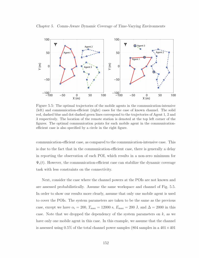
Chapter 5. Comm-Aware Dynamic Coverage of Time-Varying Environments
−100 −50 0 50 100−100
−50
0
50
100
X (m)
Y (
m)
1
2
3
4
5
6
7
8
9
10
11
12
13
14
15
16
17
18
19
20
21
22
23
24
Agent 1
Agent 2
Agent 3
−100 −50 0 50 100−100
−50
0
50
100
X (m)
Y (
m)
1
2
3
4
5
6
7
8
9
10
11
12
13
14
15
16
17
18
19
20
21
22
23
24
Agent 1
Agent 2
Agent 3
Figure 5.5: The optimal trajectories of the mobile agents in the communication-intensive(left) and communication-efficient (right) cases for the case of known channel. The solidred, dashed blue and dot-dashed green lines correspond to the trajectories of Agent 1, 2 and3 respectively. The location of the remote station is denoted at the top left corner of thefigures. The optimal communication points for each mobile agent in the communication-efficient case is also specified by a circle in the right figure.
communication-efficient case, as compared to the communication-intensive case. This
is due to the fact that in the communication-efficient case, there is generally a delay
in reporting the observation of each POI, which results in a non-zero minimum for
Ψi(t). However, the communication-efficient case can stabilize the dynamic coverage
task with less constraints on the connectivity.
Next, consider the case where the channel powers at the POIs are not known and
are assessed probabilistically. Assume the same workspace and channel of Fig. 5.5.
In order to show our results more clearly, assume that only one mobile agent is used
to cover the POIs. The system parameters are taken to be the same as the previous
case, except we have αi = 200, Tmax = 12000 s, Emax = 200 J, and ∆ = 2000 in this
case. Note that we dropped the dependency of the system parameters on k, as we
have only one mobile agent in this case. In this example, we assume that the channel
is assessed using 0.5% of the total channel power samples (804 samples in a 401×401
152

Chapter 5. Comm-Aware Dynamic Coverage of Time-Varying Environments
0 1000 2000 30000
1000
2000
3000
4000
t (s)
POI #4
Ψi(t)
0 5000 10000 150000
0.5
1
1.5
2
x 104
t (s)
POI #4
Φi(t)
Ψi(t)
Figure 5.6: The plot of Ψi(t) at the remote station for POI #4 in Fig. 5.5in communication-intensive (left) and communication-efficient (right) cases. In thecommunication-efficient case, the plot of Φi(t) at the mobile agent is also provided.
grid), which are assumed to be randomly collected during an offline survey of the
channel (see Chapter 2 for a detailed discussion on our probabilistic channel assess-
ment framework). Fig. 5.7 (left) compares the estimated and actual channel powers
at the positions of the POIs. Fig. 5.7 (right) then shows the optimal trajectory of
the mobile agent in both communication-intensive and communication-efficient cases
respectively. Note that, as proved by Theorems 5.2.1 and 5.3.1, the optimal trajec-
tory in case of a single mobile agent is the minimum-length Hamiltonian cycle, in
both communication-intensive and communication efficient cases. The optimal com-
munication point in the communication efficient case, i.e., the POI with the smallest
Γ(qi, χ) (see Section 5.3.3), is also specified by a circle in Fig. 5.7 (right). Table 5.4
lists the optimal stop times and the value of Γ(qi, χ) at all the POIs. For the sake of
comparison, this table also shows the minimum required transmit power for the case
of known channel powers, i.e., PTH
G(qi), for all the POIs. The optimal period, optimal
total energy per period, optimal motion energy per period and optimal communica-
tion energy per period, in both communication-intensive and communication-efficient
153

Chapter 5. Comm-Aware Dynamic Coverage of Time-Varying Environments
cases, are listed in Table 5.5.11 In this example, we set χ = 0.95. From Table 5.4, one
can see that Γ(qi, χ) is larger than the minimum required transmit power in case of
known channel power, i.e., PTH
G(qi), at each POI. This is to guarantee that, based on the
variance of channel estimation, the probability of connectivity is larger than χ. Note
that in Table 5.4, the optimal periods are the same for both communication-intensive
and communication-efficient cases, since we only have one mobile agent. Also, as can
be seen from Table 5.4, the optimal communication energy per period and, as a direct
result, the optimal total energy per period is larger in the communication-intensive
case, as expected (tc is taken to be the same for both cases).
5 10 15 20−70
−60
−50
−40
−30
−20
POI
GdB(qi)GdB(qi)
−100 −50 0 50 100−100
−50
0
50
100
X (m)
Y (
m)
1
2
3
4
5
6
7
8
9
10
11
12
13
14
15
16
17
18
19
20
21
22
23
24
Figure 5.7: The comparison of the estimated and real channel powers at the POIs (left)and the optimal trajectories of one mobile agent in both communication-intensive andcommunication-efficient cases and for the case of unknown channel powers (right). Thelocation of the remote station is denoted at the top left corner of the right figure. Theoptimal communication point for the mobile agent in the communication-efficient case isalso specified by a circle in the right figure. It can be seen that the optimal trajectory isthe Hamiltonian cycle over the set of POIs.
11The calculated energy values are based on assuming that the mobile agent will use the apriori found optimal channel powers, based on the probabilistic channel assessment at thePOIs. Alternatively, the agent can measure the channel at the POIs after deployment andbetter adapt its transmission powers at the POIs, resulting in less total energy consumption.
154

Chapter 5. Comm-Aware Dynamic Coverage of Time-Varying Environments
POI t∗i Γ(qi, χ)PTH
G(qi)POI t∗i Γ(qi, χ)
PTH
G(qi)
1 113.13 s 67.259 mW 21.316 mW 13 162.38 s 127.25 mW 43.702 mW2 85.084 s 122.72 mW 26.615 mW 14 91.422 s 200.61 mW 74.99 mW3 73.151 s 44.735 mW 13.532 mW 15 101.09 s 125.84 mW 27.739 mW4 155.76 s 45.637 mW 12.171 mW 16 81.005 s 36.209 mW 4.7053 mW5 159.26 s 4.1431 mW 1.6186 mW 17 131.75 s 16.905 mW 6.5547 mW6 148.9 s 71.488 mW 14.09 mW 18 74.563 s 1.338 mW 0.33904 mW7 71.034 s 49.583 mW 10.496 mW 19 99.129 s 12.229 mW 3.206 mW8 97.799 s 18.894 mW 2.9919 mW 20 152.51 s 22.329 mW 7.4526 mW9 158.17 s 28.176 mW 6.0823 mW 21 78.6 s 7.8333 mW 1.1143 mW10 108.17 s 774.54 mW 589.35 mW 22 156.13 s 224.98 mW 80.994 mW11 101.33 s 165.64 mW 39.749 mW 23 133.92 s 41.428 mW 6.118 mW12 88.73 s 185.93 mW 136.71 mW 24 116.3 s 2.1681 mW 0.96975 mW
Table 5.4: The optimal stop times (for both communication-intensive and communication-efficient cases), and the values of PTH
G(qi)and Γ(qi, χ) for all the POIs in Fig. 5.7.
Communication-Intensive Case Communication-Efficient CaseT ∗ E∗ E∗
m E∗c T ∗ E∗ E∗
m E∗c
10250 s 124.36 J 76.403 J 47.957 J 10250 s 76.43 J 76.403 J 0.02676 J
Table 5.5: The optimal period, optimal total energy per period, optimal motion energyper period and optimal communication energy per period in both communication-intensiveand communication-efficient cases and for all the mobile agents in Fig. 5.7. Note that thedependency on k has been dropped as there is one mobile agent in this case.
Fig. 5.8 (left) and Fig. 5.8 (right) show the plots of Ψi(t) at the remote station for
two sample POIs in Fig. 5.7 (POI #4 and POI #10). For the sake of comparison, each
figure shows the plots of Ψi(t) at the remote station for three cases: communication-
intensive, communication-efficient and communication-unaware. By communication-
unaware we mean the case where the same transmission power is used at all the POIs,
without adapting to channel powers. To have a fair comparison, we set this fixed
communication energy budget to be the same as the optimal communication energy
found in the communication-intensive case (47.9573 J). The transmission power at
every POI is then fixed to 1m
∑i∈V Γ(qi, χ) = 99.91 mW in this case. It can be seen
155

Chapter 5. Comm-Aware Dynamic Coverage of Time-Varying Environments
that in communication-intensive and communication-efficient cases, both of the POIs
could be stably covered. The communication-unaware case, however, could stabilize
the sensing of only one POI (POI #4). This is due to the fact that the robot is not
connected to the remote station at the position of POI #10 in the communication-
unaware case. This has been explained visually in Fig. 5.9. This figure shows the
positions of the POIs superimposed on the connectivity map to the remote station
for the communication-unaware case, assuming that the fixed transmission power of
99.91 mW is used. It can be seen that POI #10 and POI #12 are disconnected,
resulting in Ψi(t) becoming unstable at these points.
0 0.5 1 1.5 2
x 104
0
1
2
x 104
Ψi(t
)
POI #4
comm−intensive
0 0.5 1 1.5 2
x 104
1
2
3
x 104
Ψi(t
)
comm−efficient
0 0.5 1 1.5 2
x 104
0
1
2
x 104
Ψi(t
)
t (s)
comm−unaware
0 0.5 1 1.5 2
x 104
0
10000
Ψi(t
)POI #10
comm−intensive
0 0.5 1 1.5 2
x 104
0.51
1.52
2.5x 10
4
Ψi(t
)
comm−efficient
0 0.5 1 1.5 2
x 104
123
x 104
Ψi(t
)
t (s)
comm−unaware
Figure 5.8: The plots of Ψi(t) at the remote station for POI #4 (left) and POI #10 (right)in Fig. 5.7. These figures compare the time evolution of Ψi(t) in communication-intensive,communication-efficient and communication-unaware cases.
Note that after solving the proposed MILP to find the feasible stabilizing policy
in this specific example, all the POIs in the communication-intensive case or the
optimal communication point in the communication-efficient case are connected, al-
though the channel is assessed probabilistically. This may or may not be the case
in general, depending on the quality of the channel assessment, especially the power
of the multipath fading component of the channel. Since multipath fading is not
predictable using sparse sampling of the channel, one expects that by increasing the
156

Chapter 5. Comm-Aware Dynamic Coverage of Time-Varying Environments
X (m)
Y (
m)
1
2
3
4
5
6
7
8
9
10
11
12
13
14
15
16
17
18
19
20
21
22
23
24
−100 −50 0 50 100−100
−50
0
50
100
Figure 5.9: Positions of the POIs superimposed on the connectivity map to the re-mote station, assuming that the fixed transmission power 1
m
∑i∈V Γ(qi, χ) is used in the
communication-unaware case. The disconnected POIs are circled on the figure.
power of multipath fading the number of POIs that can be covered decreases. This
is shown in Fig. 5.10. Fig. 5.10 (left) shows the percentage of the connected POIs
in Fig. 5.7 that can be covered by the mobile agent in the communication-intensive
case, as a function of the power of the multipath fading component. The figure
also shows the results for the non-adaptive communication-unaware case. The com-
munication energy per period in the communication-intensive case is calculated to
guarantee for χ = 0.95. The same energy budget is then used in the communication-
unaware case, where the power is uniformly distributed among all the POIs. The
results are averaged for 500 different realizations of the channel. In this example,
the path loss and shadowing components are kept fixed and only the multipath fad-
ing component is regenerated in each realization. Similar to Fig. 5.7, the channel
is assessed using 0.5% of the total channel power samples. Interesting results can
be observed. First, it can be seen that the percentage of the POIs that can be cov-
ered in the communication-intensive case decreases as the power of multipath fading
increases. Second, for a fixed multipath power, the percentage of POIs, covered in
the communication-unaware case, is lower than the communication-intensive case,
157

Chapter 5. Comm-Aware Dynamic Coverage of Time-Varying Environments
unless multipath power is very large. Third, for a very large multipath power, the
percentage of the POIs covered by the communication-intensive case converges to
that of the communication-unaware case. These results can be justified as follows:
As the multipath fading power increases, the quality of channel assessment de-
grades considerably. Although the optimal energy allocated for communication, i.e.,∑
i∈V Γ(qi, χ), also increases as the power of multipath fading increases, the over-
all number of connected POIs decreases in the communication-intensive case. The
increase in the optimal energy allocated for communication, however, results in an
opposite effect in the communication-unaware case. Since the power is distributed
uniformly among all the POIs in this case, the increase in the allocated transmission
power, along with more randomness in channel variations, increases the chance of
connectivity at the POIs. Finally, for very large multipath fading power, adapta-
tion of the transmission power in the communication-intensive case is not effective
anymore due to large channel variations, resulting in almost the same percentage of
connected POIs as of the communication-unaware case. Note that we used Rician
multipath fading in this example. Therefore, the maximum possible multipath fad-
ing power is ω = 5.1195 dB, which corresponds to the case when Rician distribution
becomes a Raleigh distribution [54, 59]. To get a better idea about how the channel
looks like for very small and very large multipath fading powers, Fig. 5.11 shows two
sample channels with ω = 0.8730 dB (left) and ω = 5.0941 dB (right). The Rician
K-parameter (the ratio of the power of the non-multipath component to that of the
multipath component [59]) is equal to 50 for the left figure and 0.2 for the right one.
The probability of connectivity of the optimal transmission point found in the
communication-efficient case also presents a similar behavior. Fig. 5.10 (middle)
shows the plot of the probability of connectivity of the optimal transmission point in
the communication-efficient case, as a function of the multipath power. The result is
averaged over 500 realizations of the channel. Similar to the communication-intensive
158

Chapter 5. Comm-Aware Dynamic Coverage of Time-Varying Environments
case, it can be seen that the probability of connectivity decreases as multipath power
increases. Finally, Fig. 5.10 (right) shows the total optimal communication energy as
a function of multipath power for both communication-intensive and communication-
efficient cases. As expected, the energy increases as the multipath power increases.
1 2 3 4 5
0.9
0.92
0.94
0.96
0.98
ω (dB)
% o
f P
OIs
connecte
d
comm−intensivecomm−unaware
1 2 3 4 50.93
0.94
0.95
0.96
0.97
0.98
0.99
1
ω (dB)
Pro
b o
f connectivity a
t ξ* T
X
in c
om
m−
effic
ient case
1 2 3 4 5
10−1
100
101
102
ω (dB)
E∗ c
(J)
comm−intensivecomm−efficient
Figure 5.10: The percentage of the POIs that can be covered by the mobile agent ofFig. 5.7 in the communication-intensive case (left), the probability of connectivity of theoptimal transmission point in the communication-efficient case (middle), and the totaloptimal communication energy (right) as a function of multipath power.
Figure 5.11: Two sample channels with ω = 0.8730 dB (left) and ω = 5.0941 dB (right).The path loss and shadowing components of both channels are the same as in Fig. 5.4
Finally, in order to confirm the probabilistic analysis of Sections 5.2.4 and 5.3.4
for a large number of POIs, Fig. 5.12 compares the actual and theoretical average
minimum total energy per period, consumed to cover a set of POIs by one mobile
agent, as a function of the number of POIs. Fig. 5.13 (left) and Fig. 5.13 (right) also
show the average minimum communication energy per period for communication-
intensive and communication-efficient cases respectively. The results for every m are
159

Chapter 5. Comm-Aware Dynamic Coverage of Time-Varying Environments
calculated by averaging over 500 different channels and sets of POIs. The POIs are
distributed according to a uniform pdf over the workspace of Fig. 5.7. The channel
in the dB domain is generated using a Gaussian distribution, with a mean equal to
the path loss component of the channel of Fig. 5.5 and a standard deviation equal
to ϑ = 5 dB. Also, in this example we set Ploss,m = Ploss,s = Ploss = 0.1 mW, ρ = 1
and α = 200 for all the POIs. The rest of the parameters are the same as in Fig.
5.5. Note that we dropped the dependency of the parameters on i and k as there is
only one mobile agent and the parameters are the same for all the POIs. Fig. 5.13
shows that the average minimum communication energy per period is an increasing
function of the number of POIs in the communication-intensive case, as expected.
However, it is a decreasing function of the number of POIs in the communication-
efficient case. This is explained by the fact that by increasing the number of POIs
in an environment, the chance of finding a higher channel power at one of the POIs
increases. Also, it can be seen that overall the theoretical values provide a good
approximation to the simulated ones.
20 30 40 50 60 70
80
100
120
140
160
180
# of POIs
Em
in,ave
(J)
actual (comm−intensive)theoretical (comm−intensive)actual (comm−efficient)theoretical (comm−efficient)
Figure 5.12: The actual and theoretical average minimum total energy consumed in eachperiod to cover a set of POIs, as a function of the number of POIs.
160

Chapter 5. Comm-Aware Dynamic Coverage of Time-Varying Environments
20 30 40 50 60 70
20
25
30
35
40
45
50
55
# of POIs
ET
X,m
in,ave
(J)
actualtheoretical
20 30 40 50 60 70
4
6
8
10
12
x 10−3
# of POIs
ET
X,m
in,ave
(J)
actualtheoretical
Figure 5.13: The actual and theoretical average minimum communication energy con-sumed in each period to cover a set of POIs as a function of the number of POIs, in thecommunication-intensive (left) and communication-efficient (right) cases.
5.5 Further Extension of the Dynamic Coverage
Problem
In this section, we extend our dynamic coverage results by considering a non-zero
range for the sensing/actuation device of the mobile agents and adapting their ve-
locities and transmission rates (in addition to their transmission powers) along their
trajectories. Unlike our previous results, here we take into account the number of
information bits that are transmitted to and correctly received by the remote sta-
tion. We, however, assume only one robot in this section to facilitate mathematical
derivations.12
We assume an obstacle-free workspace W ⊂ R2, which contains a set of m POIs
Q = q1, · · · , qm ⊂ W. Let V = 1, · · · , m denotes the indices of the POIs. In
this section, we specifically consider a scenario where information bits are generated
with certain rates at the POIs (e.g., consider the case where the POIs are data
loggers that are distributed over the workspace to log time variations of a physical
12Extension to the case of multiple mobile agents in this case is under our consideration.
161
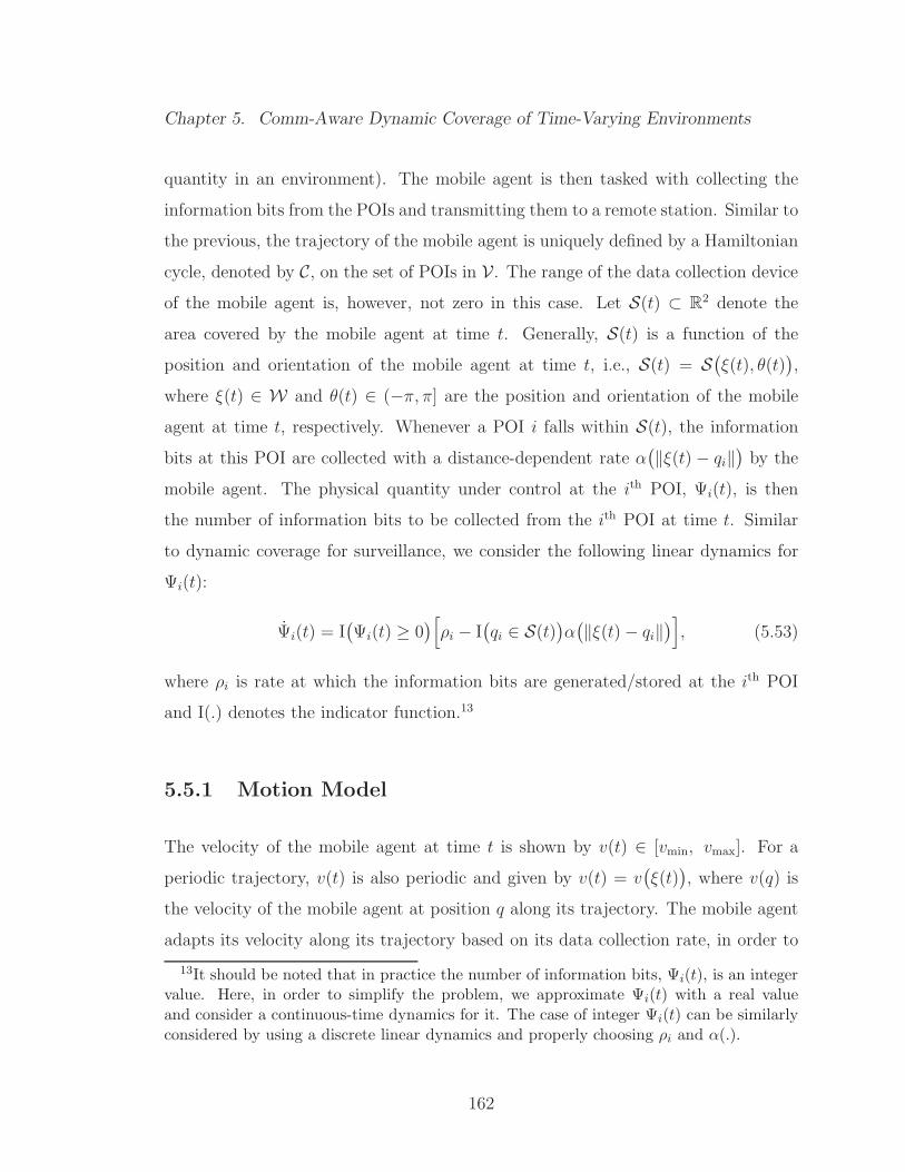
Chapter 5. Comm-Aware Dynamic Coverage of Time-Varying Environments
quantity in an environment). The mobile agent is then tasked with collecting the
information bits from the POIs and transmitting them to a remote station. Similar to
the previous, the trajectory of the mobile agent is uniquely defined by a Hamiltonian
cycle, denoted by C, on the set of POIs in V. The range of the data collection device
of the mobile agent is, however, not zero in this case. Let S(t) ⊂ R2 denote the
area covered by the mobile agent at time t. Generally, S(t) is a function of the
position and orientation of the mobile agent at time t, i.e., S(t) = S(ξ(t), θ(t)
),
where ξ(t) ∈ W and θ(t) ∈ (−π, π] are the position and orientation of the mobile
agent at time t, respectively. Whenever a POI i falls within S(t), the information
bits at this POI are collected with a distance-dependent rate α(‖ξ(t)− qi‖
)by the
mobile agent. The physical quantity under control at the ith POI, Ψi(t), is then
the number of information bits to be collected from the ith POI at time t. Similar
to dynamic coverage for surveillance, we consider the following linear dynamics for
Ψi(t):
Ψi(t) = I(Ψi(t) ≥ 0
)[ρi − I
(qi ∈ S(t)
)α(‖ξ(t)− qi‖
)], (5.53)
where ρi is rate at which the information bits are generated/stored at the ith POI
and I(.) denotes the indicator function.13
5.5.1 Motion Model
The velocity of the mobile agent at time t is shown by v(t) ∈ [vmin, vmax]. For a
periodic trajectory, v(t) is also periodic and given by v(t) = v(ξ(t)
), where v(q) is
the velocity of the mobile agent at position q along its trajectory. The mobile agent
adapts its velocity along its trajectory based on its data collection rate, in order to
13It should be noted that in practice the number of information bits, Ψi(t), is an integervalue. Here, in order to simplify the problem, we approximate Ψi(t) with a real valueand consider a continuous-time dynamics for it. The case of integer Ψi(t) can be similarlyconsidered by using a discrete linear dynamics and properly choosing ρi and α(.).
162
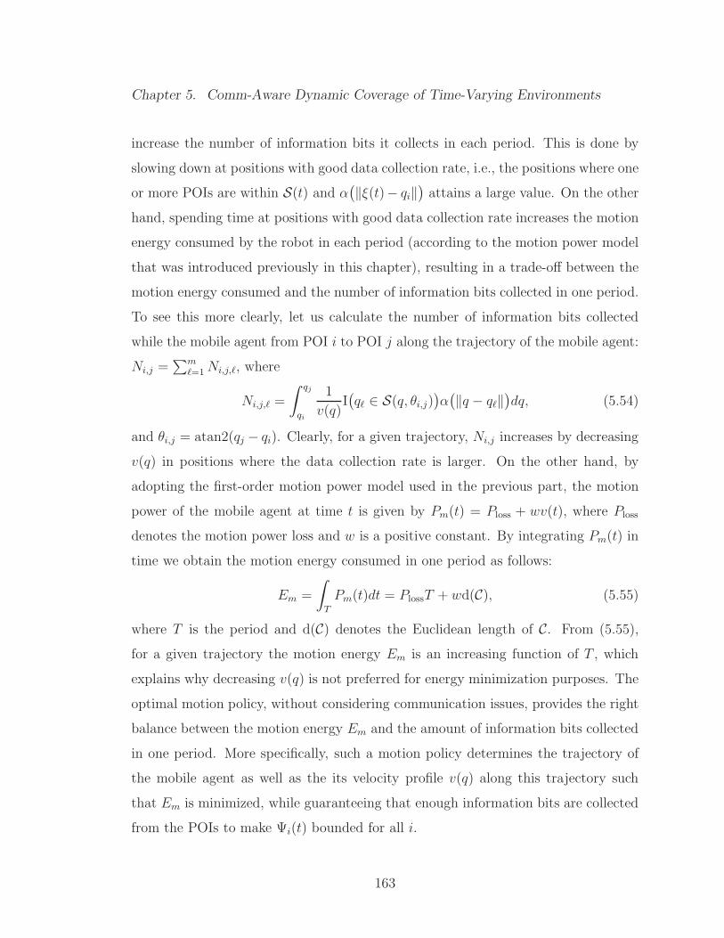
Chapter 5. Comm-Aware Dynamic Coverage of Time-Varying Environments
increase the number of information bits it collects in each period. This is done by
slowing down at positions with good data collection rate, i.e., the positions where one
or more POIs are within S(t) and α(‖ξ(t)− qi‖
)attains a large value. On the other
hand, spending time at positions with good data collection rate increases the motion
energy consumed by the robot in each period (according to the motion power model
that was introduced previously in this chapter), resulting in a trade-off between the
motion energy consumed and the number of information bits collected in one period.
To see this more clearly, let us calculate the number of information bits collected
while the mobile agent from POI i to POI j along the trajectory of the mobile agent:
Ni,j =∑m
ℓ=1Ni,j,ℓ, where
Ni,j,ℓ =
∫ qj
qi
1
v(q)I(qℓ ∈ S(q, θi,j)
)α(‖q − qℓ‖
)dq, (5.54)
and θi,j = atan2(qj − qi). Clearly, for a given trajectory, Ni,j increases by decreasing
v(q) in positions where the data collection rate is larger. On the other hand, by
adopting the first-order motion power model used in the previous part, the motion
power of the mobile agent at time t is given by Pm(t) = Ploss + wv(t), where Ploss
denotes the motion power loss and w is a positive constant. By integrating Pm(t) in
time we obtain the motion energy consumed in one period as follows:
Em =
∫
T
Pm(t)dt = PlossT + wd(C), (5.55)
where T is the period and d(C) denotes the Euclidean length of C. From (5.55),
for a given trajectory the motion energy Em is an increasing function of T , which
explains why decreasing v(q) is not preferred for energy minimization purposes. The
optimal motion policy, without considering communication issues, provides the right
balance between the motion energy Em and the amount of information bits collected
in one period. More specifically, such a motion policy determines the trajectory of
the mobile agent as well as the its velocity profile v(q) along this trajectory such
that Em is minimized, while guaranteeing that enough information bits are collected
from the POIs to make Ψi(t) bounded for all i.
163

Chapter 5. Comm-Aware Dynamic Coverage of Time-Varying Environments
5.5.2 Communication Model
The information bits collected from the POIs are transmitted to the remote sta-
tion along the trajectory of the mobile agent. Unlike our previous dynamic coverage
results, in this case it is important to consider how the information bits are transmit-
ted to the remote station. The mobile agent is capable of adapting its transmission
power and rate based on the quality of the channel to the remote station. By doing
so, it can control the number of information bits sent in each period, its consumed
communication energy, and the reception quality of the remote station.
We assume that MQAM modulation with nr different constellation sizes is used
by the onboard digital communication device of the mobile agent. Then, by assuming
a transmission bandwidth B, we achieve the spectral efficiency of RTX,ℓ bits/symbol
(bits/s/Hz) or equivalently the transmission rate of BRTX,ℓ bits/s by choosing the
constellation size 2RTX,ℓ , for ℓ = 1, · · · , nr [59]. Let PTX(t) and RTX(t) denote the
transmission power and the spectral efficiency chosen at time t. Then, the number
of information bits transmitted to the remote station in one period is given by
Nc = B
∫
T
RTX(t)dt. (5.56)
The communication energy consumed in one period is also
Ec =
∫
T
PTX(t)dt. (5.57)
Note that for a periodic trajectory, PTX(t) = PTX
(ξ(t)
)and RTX(t) = RTX
(ξ(t)
),
where PTX(q) and RTX(q) ∈ 0, RTX,1, · · · , RTX,nr are the transmission power and
the spectral efficiency chosen at position q along the trajectory of the mobile agent.
The reception quality at the remote station is measured by the resulting BER. For
an MQAM modulation, the BER at time t at the remote station is given by
BER(t) ≈ 0.2 exp
(− 1.5PTX(t)G(t)(
2RTX(t) − 1)BN0
), (5.58)
164

Chapter 5. Comm-Aware Dynamic Coverage of Time-Varying Environments
where G(t) = G(ξ(t)
), G(q) is the channel power at position q along the trajectory
of the mobile agent and N0
2is the PSD of the thermal noise at the receiver of the
remote station. The optimal communication policy, without considering motion
issues, then determines the trajectory of the robot, as well as PTX(q) and RTX(q)
along this trajectory, such that the communication energy Ec is minimized and all the
information bits collected in one period are transmitted to the remote station, in the
same period, with a BER lower than a given threshold BERTH. Note that optimizing
the motion and communication cannot be done independently. The trajectory of
the robot affects both Em and Ec. Furthermore, the velocity profile of the robot
determines the number of the information bits collected in one period, which affects
the transmission power and rate required for the transmission. In the next section, we
formulate our proposed combined motion and communication optimization problem.
Then, in Section 5.6.2, we show how to solve this problem using an MILP.
Before presenting our MILP, we should note that the channel power G(q) may
not be deterministically known everywhere, as we also explained in Section 5.2.3.
Furthermore, even if the channel is deterministically known, pre-planning based on
the rapidly changing multipath fading component of the channel is not preferred
in practical applications. In such case, instead of a deterministic G(q), the pdf of
G(q), given by our channel assessment framework of Chapter 2, is used to calcu-
late PBER(t) ≤ BERTH
. Then, PTX(q) and RTX(q) are selected to guarantee
PBER(t) ≤ BERTH
≥ 1 − ǫ, for a small ǫ, whenever PTX(t) > 0 and RTX(t) > 0.
This is explained in more details in Section 5.6.2.
5.6 Extended Dynamic Coverage of Time-Varying
Environments
In this section, we formulate the problem of dynamic coverage for information collec-
tion in time-varying environments, which requires adapting the velocity, transmission
165

Chapter 5. Comm-Aware Dynamic Coverage of Time-Varying Environments
power and transmission rate of the mobile agent along its trajectory. We then pro-
pose an MILP to find the optimal solution of the problem. We furthermore analyze
the solution of the MILP and its special cases mathematically.
5.6.1 Problem Formulation
Based on the discussions of the previous sections, the dynamic coverage policy for
information collection in time-varying environments is defined as follows
Definition 5.6.1. A dynamic coverage policy for information collection in a time-
varying environment using a single mobile agent is a tuple P = (C, PTX, RTX, v),
where C denote the Hamiltonian cycle defined on the set of POIs and functions PTX :
W → R≥0, RTX : W → 0, RTX,1, · · · , RTX,nr and v : W → [vmin, vmax] determine
the transmission power, spectral efficiency and velocity of the mobile agent for any
position q ∈ W along the trajectory defined by C, respectively.
Our goal in this section is then to determine the dynamic coverage policy P such
that the total energy E = Em + Ec is minimized and the following hold:
1. There exist Ψ ≥ 0 such that Ψi(t) ≤ Ψ for all t ≥ 0 and i = 1, · · · , m.
2. All the information bits collected in one period are transmitted to the remote
station, in the same period, and PBER(t) ≤ BERTH
≥ 1 − ǫ whenever
PTX(t) > 0 and RTX(t) > 0.
3. The total information bits collected in one period is no larger than the maxi-
mum memory size of the the mobile agent Lmax.
The first condition implies that the dynamical system (5.53) is stable for all POIs.
166

Chapter 5. Comm-Aware Dynamic Coverage of Time-Varying Environments
In Section 5.2 we showed that this is equivalent to the following:
Tρi −∫
T
I(qi ∈ S(t)
)α(‖ξ(t)− qi‖
)dt ≤ 0, i = 1, · · · , m, (5.59)
which implies that the total information bits collected from the ith POI is no smaller
that the number of bits generated at this POI. Furthermore, if this condition holds,
the total information bits collected in one period becomes T∑m
i=1 ρi. Therefore, the
first part of the second condition is equivalent to Nc = B∫TRTX(t)dt ≥ T
∑mi=1 ρi.
Finally, the third condition implies that T∑m
i=1 ρi ≤ Lmax. The optimization prob-
lem to solve is then given as follows:
Problem 5.6.1. The minimum-energy dynamic coverage policy for information col-
lection in a time-varying environment is given as follows:
minP
∫
T
PTX(t)dt+ PlossT + wd(C),
s.t.
1) Tρi −∫
T
I(qi ∈ S(t)
)α(‖ξ(t)− qi‖
)dt ≤ 0, ∀i = 1, · · · , m
2) B
∫
T
RTX(t)dt ≥ T
m∑
i=1
ρi,
3) if PTX(t) > 0 and RTX(t) > 0 then PBER(t) ≤ BERTH
≥ 1− ǫ, ∀t ≥ 0,
4) Tm∑
i=1
ρi ≤ Lmax, (5.60)
where T the period of movement, which is a function of the velocity profile of the
mobile agent v(t). Furthermore, v(t) = v(ξ(t)
), PTX(t) = PTX
(ξ(t)
), and RTX(t) =
RTX
(ξ(t)
).
As can be seen, Problem 5.6.1 is generally complicated to solve. Next, we show
how to solve this problem by discretizing the trajectory of the mobile agent and by
using an MILP.
167

Chapter 5. Comm-Aware Dynamic Coverage of Time-Varying Environments
5.6.2 Optimal Solution of the Dynamic Coverage in Case of
Non-zero Ranges and Adaptive Velocities, Transmis-
sion Powers and Transmission Rates
Let us discretize each possible trajectory of the mobile agent into a number of small
line segments with maximum length δmax and minimum length δmin. δmax is selected
small enough such that the channel can be considered stationary along each seg-
ment.14 Define binary variables zi,j ∈ 0, 1 such that zi,j = 1 when C includes a
path from POI i to POI j, and zi,j = 0 otherwise. Let Li,j,k denote the kth line
segment along the path from POI i to POI j. Also, let ni,j denote the number
of such line segments. Define the continuous variables τi,j,k,ℓ as the amount of time
that mobile agent transmits information bits with the spectral efficiency of RTX,ℓ, for
ℓ = 1, · · · , nr, along Li,j,k. Also, define the continuous variables i,j,k as the inverse
of the constant velocity of the mobile agent along Li,j,k. We set i,j,k = 0 whenever
zi,j = 0, which can be guaranteed by the linear constraints zi,jv−1max ≤ i,j,k ≤ zi,jv
−1min.
Based on the definition of these variable we have
∫
T
I(qℓ ∈ S(t)
)α(‖ξ(t)− qℓ‖
)dt =
m∑
i=1
m∑
j=1j 6=i
zi,jNi,j,ℓ. (5.61)
We can then confirm that the first condition in Problem 5.6.1 is equivalent to the
following for all ℓ = 1, · · · , m:
m∑
i=1
m∑
j=1j 6=i
ni,j∑
k=1
νi,j,k,ℓ i,j,k − ρℓ
m∑
i=1
m∑
j=1j 6=i
ni,j∑
k=1
di,j,k i,j,k ≥ 0, (5.62)
where the weights νi,j,k,ℓ are given by
νi,j,k,ℓ =
∫
Li,j,k
I(qℓ ∈ S(q, θi,j)
)α(‖q − qℓ‖
)dq. (5.63)
14Note that in practical applications pre-planning based on rapidly-changing multipathfading is not desired.
168

Chapter 5. Comm-Aware Dynamic Coverage of Time-Varying Environments
Here, di,j,k denotes the length of Li,j,k. Similarly, the second condition in Problem
5.6.1 is equivalent to the following:
m∑
i=1
m∑
j=1j 6=i
ni,j∑
k=1
nr∑
ℓ=1
RTX,ℓ τi,j,k,ℓ ≥∑m
i=1 ρiB
m∑
i=1
m∑
j=1j 6=i
ni,j∑
k=1
di,j,ki,j,k. (5.64)
Finally, for the third condition in Problem 5.6.1 we have
m∑
i=1
m∑
j=1j 6=i
ni,j∑
k=1
di,j,k i,j,k ≤Lmax∑mi=1 ρi
. (5.65)
The motion and communication energies can also be found as functions of the newly
defined variables. For the motion energy we have
Em = Ploss
m∑
i=1
m∑
j=1j 6=i
ni,j∑
k=1
di,j,k i,j,k + wm∑
i=1
m∑
j=1j 6=i
di,j zi,j, (5.66)
where di,j = ‖qi−qj‖. Given the transmission times τi,j,k,ℓ, the communication energy
to be minimized is also the minimum required communication energy to guarantee
PBER(t) ≤ BERTH
≥ 1−ǫ along each line segment Li,j,k for which
∑nr
ℓ=1 τi,j,k,ℓ > 0.
We have
PBER(t) ≤ BERTH
= P
G(t) ≥ κ
(2RTX(t) − 1)
PTX(t)
, (5.67)
where κ , − log(5BERTH)BN0
1.5. Assume that the channel is known only at a number of
a priori channel measurements. According to the channel assessment framework of
Chapter 2, the distribution of G(q) in the dB domain, conditioned on the channel
measurements, is given by a Gaussian pdf with mean GdB(q) and variance σ2(q). Note
that similar to dynamic coverage for for surveillance, we dropped the dependency
of the channel assessment to t and k, since there is only one mobile agent and the
channel is assessed before the operation starts. Along each line segment the channel
is stationary and, therefore, GdB(q) and σ2(q) can be assumed constant. Let us define
G(q) , 10GdB(q)
10 . Also, let Gi,j,k and σi,j,k denote the constant values of G(q) and
169

Chapter 5. Comm-Aware Dynamic Coverage of Time-Varying Environments
σ(q) along Li,j,k, respectively. After some straightforward calculations, we can then
find the minimum required communication energy, that guarantees PBER(t) ≤
BERTH
≥ 1− ǫ along each Li,j,k for which
∑nr
ℓ=1 τi,j,k,ℓ > 0, as follows:
Ec = κ
m∑
i=1
m∑
j=1j 6=i
ni,j∑
k=1
nr∑
ℓ=1
τi,j,k,ℓ(2RTX,ℓ − 1)
Gi,j,k
, (5.68)
where Gi,j,k , Gi,j,k10Q−1(1−ǫ)σi,j,k
10 and Q−1(.) denotes the inverse of the Q-function
(the tail probability of the Gaussian distribution).
The total transmission time in each segment, i.e.,∑m
ℓ=1 τi,j,k,ℓ, determines how
much time in each segment is dedicated to communication. Generally, two dif-
ferent types of constraints can be considered on∑nr
ℓ=1 τi,j,k,ℓ. The first type of
constraints guarantee that∑nr
ℓ=1 τi,j,k,ℓ is no larger than a fixed transmission time
tc ≤ mini,j,kdi,j,kvmax
:
Type I constraints:nr∑
ℓ=1
τi,j,k,ℓ ≤ zi,jtc, ∀i, j, k. (5.69)
The total transmission time in each segment is not affected by the velocity of the mo-
bile agent in this case. The second type of constraints, on the other hand, guarantee∑nr
ℓ=1 τi,j,k,ℓ is no larger than the time required to move along Li,j,k:
Type II constraints:nr∑
ℓ=1
τi,j,k,ℓ ≤ di,j,k i,j,k, ∀i, j, k, (5.70)
where we set i,j,k = 0 whenever zi,j = 0. By adding the second type of constraints,
the velocity of the mobile agent along its trajectory affects not only data collection
but also data transmission. This is due to the fact that by increasing i,j,k in some
areas (e.g. areas with good channel quality) more information bits can be transmitted
to the remote station.
Based on the discretized version of Problem 5.6.1, we then propose the MILP of
Program 3 for finding the optimal dynamic coverage policy.
170

Chapter 5. Comm-Aware Dynamic Coverage of Time-Varying Environments
Program 3 MILP for solving Problem 5.6.1
min E = Em + Ec = Ploss
∑mi=1
∑mj=1j 6=i
∑ni,j
k=1 di,j,k i,j,k + w∑m
i=1
∑mj=1j 6=i
di,j zi,j
+κ∑m
i=1
∑mj=1j 6=i
∑ni,j
k=1
∑nr
ℓ=1 τi,j,k,ℓ(2
RTX,ℓ−1)
Gi,j,k
1)∑m
i=1
∑mj=1j 6=i
∑ni,j
k=1 νi,j,k,ℓ i,j,k − ρℓ∑m
i=1
∑mj=1j 6=i
∑ni,j
k=1 di,j,k i,j,k ≥ 0, ∀ℓ,
2)∑m
i=1
∑mj=1j 6=i
∑ni,j
k=1
∑nr
ℓ=1RTX,ℓ τi,j,k,ℓ ≥∑m
i=1 ρiB
∑mi=1
∑mj=1j 6=i
∑ni,j
k=1 di,j,ki,j,k,
3)∑m
i=1
∑mj=1j 6=i
∑ni,j
k=1 di,j,k i,j,k ≤ Lmax∑mi=1 ρi
,
4)∑nr
ℓ=1 τi,j,k,ℓ ≤ zi,jtc or∑nr
ℓ=1 τi,j,k,ℓ ≤ di,j,k i,j,k, ∀i, j, k,5) zi,jv
−1max ≤ i,j,k ≤ zi,jv
−1min, ∀i, j, k,
6)∑m
j=1j 6=i
zi,j = 1,∑m
j=1j 6=i
zj,i = 1, ∀i,
7) ui − uj + (m− 1)zi,j ≤ (m− 2), ∀i 6= 1, j 6= 1,
8) 2 ≤ ui ≤ m, ∀i 6= 1,
9) zi,j ∈ 0, 1, τi,j,k,ℓ ∈ R≥0, i,j,k ∈ R≥0, ui ∈ Z≥0,
Here, we have introduced m−1 extra integer variables u2, · · · , um. In this MILP,
in addition to constraints 1 to 5, which we introduced previously, constraint 6 enforces
each POI to have exactly one degree in and one degree out. Constraints 7 and 8 are
the Miller-Tucker-Zemlin (MTZ) constraints [106,111], which are added to eliminate
the subtours. This MILP can be solved using several efficient solvers, such as IBM
ILOG CPLEX [104] and SAS/OR [105].
Note that the optimal transmission times τi,j,k,ℓ, given by the solution of the MILP
of Program 3, are sufficient to find the optimal transmission power and transmission
rate profiles. More specifically, along any line segment Li,j,k and for ℓ = 1, · · · , nr,
we set the transmission power to κ2RTX,ℓ−1Gi,j,k
and transmit the information bits with
the spectral efficiency of RTX,ℓ for time interval τi,j,k,ℓ, if τi,j,k,ℓ > 0. Therefore, by
discretizing Problem 5.6.1, the solution of this MILP uniquely gives the optimal P.
171

Chapter 5. Comm-Aware Dynamic Coverage of Time-Varying Environments
Also, note that the concept of virtual POIs, introduced in Section 5.3, can be also
used in this case as well. The virtual POIs are located at regions with good channel
qualities which are also close to the actual POIs. By ensuring that the mobile agent
passes through these points, we can then decrease the optimal communication energy
considerably.
5.6.3 Mathematical Analysis and Special Cases
In this section, we mathematically analyze the solution of the MILP of Program 3
and its special cases. We present our results in the form of the following theorems:
Theorem 5.6.1. Assume that the trajectory of the mobile agent is given by a Hamil-
tonian cycle C beforehand. Also, assume that the constraints in (5.69) are used for
the total transmission time in each segment. Then, the following are true:
1. The optimal velocity profile along the trajectory is given by the following linear
program (LP):
min∑
(i,j)∈C
ni,j∑
k=1
di,j,ki,j,k (5.71)
s.t.
1)∑
(i,j)∈C
ni,j∑
k=1
(νi,j,k,ℓ − ρℓdi,j,k
)i,j,k ≥ 0, ∀ℓ,
2)∑
(i,j)∈C
ni,j∑
k=1
di,j,ki,j,k ≤Lmax∑mi=1 ρi
,
3) v−1max ≤ i,j,k ≤ v−1
min, ∀i, j, k.
2. The optimal transmission time profile along the trajectory is given by the fol-
172

Chapter 5. Comm-Aware Dynamic Coverage of Time-Varying Environments
lowing LP:
min∑
(i,j)∈C
ni,j∑
k=1
nr∑
ℓ=1
τi,j,k,ℓ(2RTX,ℓ − 1)
Gi,j,k
(5.72)
s.t.
1)∑
(i,j)∈C
ni,j∑
k=1
nr∑
ℓ=1
RTX,ℓτi,j,k,ℓ ≥∑m
i=1 ρiB
T ∗,
2)
nr∑
ℓ=1
τi,j,k,ℓ ≤ tc, ∀i, j, k,
where T ∗ =∑
(i,j)∈C∑ni,j
k=1 di,j,k∗i,j,k is the optimal period found using the solu-
tion of (5.71).
3. In the optimal solution, v∗i,j,k = vmax in any segment for which∑m
ℓ=1 νi,j,k,ℓ = 0.
In other segments, the optimal velocities are the maximum possible velocities
that do not violate the stability constraint (5.62).
4. In the optimal solution,∑nr
ℓ=1 τ∗i,j,k,ℓ > 0 only in a number of segments where
Gi,j,k is the largest. Also, if for two segments (i1, j1, k1) and (i2, j2, k2) we have
Gi1,j1,k1 > Gi2,j2,k2, then, necessarily,
nr∑
ℓ=1
τ ∗i1,j1,k1,ℓ(2RTX,ℓ − 1
)≥
nr∑
ℓ=1
τ ∗i2,j2,k2,ℓ(2RTX,ℓ − 1
). (5.73)
Proof. In case the trajectory of the mobile agent is given and the constraints in (5.69)
are used for the total transmission time in each segment, the problem of optimizing
the velocity and transmission times becomes decoupled. The velocity of the mobile
agent is then found to minimize the motion energy and the total information bits
collected in one period, while meeting the constraints on the stability and the total
memory size. Note that minimizing the number of collected information bits is in
favor of minimizing the communication energy and, as a direct result, the total
energy. In case the trajectory is given, the motion energy as well as the number of
173

Chapter 5. Comm-Aware Dynamic Coverage of Time-Varying Environments
information bits collected are minimized when the period is minimized. This results
in the LP of (5.71) for finding the optimal velocity profile in the first part of the
theorem. The resulting optimal period is then used to find the optimal transmission
times such that the total communication energy is minimized, resulting in the LP of
(5.72) in the second part of the theorem.
From (5.71), it is clear that whenever∑m
ℓ=1 νi,j,k,ℓ = 0 in a segment, i.e., when-
ever none of the POIs are being covered by the onboard data collection device of the
mobile agent, the optimal velocity is necessarily vmax such that the period is mini-
mized. Furthermore, in the other segments, where at least one of the POIs is covered,
the optimal velocities are the maximum possible velocities that do not violate the
stability constraint. This proves third part of the theorem.
The proof of the forth part is by contradiction. Consider two segments (i1, j1, k1)
and (i2, j2, k2) for which Gi1,j1,k1 > Gi2,j2,k2. Assume that for these two segments∑nr
ℓ=1 τ∗i1,j1,k1,ℓ
(2RTX,ℓ − 1
)<∑nr
ℓ=1 τ∗i2,j2,k2,ℓ
(2RTX,ℓ − 1
). Then, if the optimal trans-
mission times of segment (i1, j1, k1) are used for segment (i2, j2, k2) instead and vice
versa, none of the constraints of (5.72) are violated. However, the total communica-
tion energy becomes smaller, since
nr∑
ℓ=1
τ ∗i1,j1,k1,ℓ(2RTX,ℓ − 1)
Gi1,j1,k1
+nr∑
ℓ=1
τ ∗i2,j2,k2,ℓ(2RTX,ℓ − 1)
Gi2,j2,k2
−nr∑
ℓ=1
τ ∗i1,j1,k1,ℓ(2RTX,ℓ − 1)
Gi2,j2,k2
−nr∑
ℓ=1
τ ∗i2,j2,k2,ℓ(2RTX,ℓ − 1)
Gi1,j1,k1
(5.74)
=
(1
Gi2,j2,k2
− 1
Gi1,j1,k1
)( nr∑
ℓ=1
τ ∗i2,j2,k2,ℓ(2RTX,ℓ − 1
)−
nr∑
ℓ=1
τ ∗i1,j1,k1,ℓ(2RTX,ℓ − 1
))> 0.
This is a contradiction which proves the forth part of the theorem.
From Theorem 5.6.1, by choosing the constraints in (5.69) and by assuming a
given trajectory, the problem of finding the optimal motion and communication
174

Chapter 5. Comm-Aware Dynamic Coverage of Time-Varying Environments
policies becomes decoupled. This is, however, not the case when the constraints in
(5.70) are used for the total transmission time in each segment.
Next, we consider the special case of the MILP of Program 3 when the area
covered by the onboard data collection device of the mobile agent is very small, i.e.,
|S(t)| = 0. In this case, the mobile agent can only collect the information bits at the
positions of the POIs. The dynamics of Ψi(t) is given by the following in this case,
which is similar to the one considered in Section 5.1:
Ψi(t) = I(Ψi(t) ≥ 0
)[ρi − I
(ξ(t) = qi
)α0
], (5.75)
where we have defined α0 , α(0). As explained in Section 5.1, in order to guarantee
the boundedness of the Ψi(t), the mobile agent is then required to stop for some time
at each POI. Let ti denote the stop time at the ith POI. Given the trajectory of the
mobile agent, the optimal velocity and stop times at the POIs are then given by the
following lemma in this case:
Lemma 5.6.1. Assume that the trajectory of the mobile agent is given by a Hamil-
tonian cycle C and∑m
i=1 ρi < α0. Then the following hold in the case of |S(t)| = 0:
1. If the constraints in (5.69) are used for the total transmission time in each seg-
ment, the optimal motion policy, which minimizes the total energy and guar-
antees the boundedness of Ψi(t) for all i = 1, · · · , m, is to choose the fixed
maximum velocity vmax for moving along the trajectory and to stop at the ith
POI for time t∗i =ρiφα0
d(C)vmax
, where φ , 1− 1α0
∑mi=1 ρi.
2. If the constraints in (5.70) are used for the total transmission time in each seg-
ment, the optimal motion is not necessarily to move with the maximum velocity
along the trajectory. Also, for a given velocity profile along the trajectory, the
optimal stop time at POI i is t∗i =ρiφα0
∑(i,j)∈C
∑ni,j
k=1 di,j,k i,j,k.
175

Chapter 5. Comm-Aware Dynamic Coverage of Time-Varying Environments
Proof. The proof is similar to the proof of Theorem 5.2.1 and is omitted for brevity.
Using Lemma 5.6.1, the MILP of Program 3 can be modified to find the opti-
mal motion and communication policies in the case of |S(t)| = 0, as shown by the
following two theorems:
Theorem 5.6.2. Assume that the constraints in (5.69) are used for the total trans-
mission time in each segment. Then, the optimal motion policy is to move with the
maximum velocity vmax. Also, the optimal trajectory and transmission times in the
case of |S(t)| = 0 are given by the following MILP:
min w
m∑
i=1
m∑
j=1j 6=i
zi,jdi,j + κ
m∑
i=1
m∑
j=1j 6=i
ni,j∑
k=1
nr∑
ℓ=1
τi,j,k,ℓ(2RTX,ℓ − 1)
Gi,j,k
s.t.
1)m∑
i=1
m∑
j=1j 6=i
ni,j∑
k=1
nr∑
ℓ=1
RTX,ℓτi,j,k,ℓ ≥1
B
∑mi=1 ρi
φvmax
m∑
i=1
m∑
j=1j 6=i
zi,jdi,j,
2)
∑mi=1 ρi
φvmax
m∑
i=1
m∑
j=1j 6=i
zi,jdi,j ≤ Lmax,
3)nr∑
ℓ=1
τi,j,k,ℓ ≤ zi,jtc, ∀i, j, k,
4) Constraints 6, 7, 8 and 9 in MILP of Program 3, (5.76)
where w , 1φPloss
vmax+ w.
Proof. The proof is based on the fact that in this case the minimum period T required
for stability is given by T = 1φvmax
∑mi=1
∑mj=1j 6=i
zi,jdi,j. This results in the following
motion energy in each period: Em = w∑m
i=1
∑mj=1j 6=i
zi,jdi,j. By substituting T and
Em in Program 3, the MILP of (5.76) results.
176

Chapter 5. Comm-Aware Dynamic Coverage of Time-Varying Environments
Note that by setting T ∗ = d(C)φvmax
, the results of parts 2 and 4 of Theorem 5.6.1
hold for the MILP of (5.76) as well.
Theorem 5.6.3. Assume that the constraints in (5.70) are used for the total trans-
mission time in each segment. Then, the MILP, that gives the optimal motion and
communication policies in the case of |S(t)| = 0, is the same MILP of Program
3, without the stability constraints in (5.62) and after replacing i,j,k with 1φi,j,k in
(5.64), (5.65) and (5.66).
Proof. In case the constraints in (5.70) are used for the total transmission time
in each segment, the minimum period T required for stability is given by T =
1φ
∑mi=1
∑mj=1j 6=i
∑ni,j
k=1 di,j,ki,j,k. By substituting T in the MILP of Program 3 and re-
moving the constraints on stability (the stability is already guaranteed by choosing
proper stop times), it becomes clear that the optimal policies are the solution of the
this MILP without the stability constraints and after replacing i,j,k with 1φi,j,k.
Another special case happens when the mobile agent is forced to transmits its
collected information bits at the positions of the POIs only. This may be the case
when the actual POIs are located in a region with a poor channel quality and a
number of virtual POIs are added to improve the communication. In this case,
the mobile agent needs to stop for some time at a number of POIs to transmit its
collected information bits. Let τi,ℓ represent the time spent for transmission with
the spectral efficiency of RTX,ℓ at the ith POI. The following theorem then gives the
optimal motion and communication policies in this case, when we additionally have
|S(t)| = 0:
Theorem 5.6.4. Assume that the mobile agent only transmits at the location of the
POIs and |S(t)| = 0. Then, the following hold:
1. The optimal trajectory is given by the minimum-length Hamiltonian cycle on
177

Chapter 5. Comm-Aware Dynamic Coverage of Time-Varying Environments
the POIs, H, which is given by the solution of a Traveling Salesman Problem
(TSP). Also, the optimal velocity along the trajectory is vmax.
2. The optimal stop times and transmission times are given by the solution of the
following LP:
min Ploss
m∑
i=1
ti + κ
m∑
i=1
nr∑
ℓ=1
τi,ℓ(2RTX,ℓ − 1)
Gi
s.t.
1) α0ti − ρi
(d(H)
vmax+
m∑
i=1
ti
)≥ 0, ∀i,
2)
m∑
i=1
nr∑
ℓ=1
τi,ℓ RTX,ℓ ≥∑m
i=1 ρiB
(d(H)
vmax+
m∑
i=1
ti
),
3)nr∑
ℓ=1
τi,ℓ ≤ ti, ∀i,
4) τi,ℓ ≥ 0, ti ≥ 0, ∀i, ℓ, (5.77)
where Gi , G(qi)10Q−1(1−ǫ)σ(qi)
10 .
Proof. Since, the trajectory of the mobile agent affects neither the data collection
nor the data transmission, the optimal trajectory which results in the minimum
total energy is simply the one that results in the minimum period. This happens
after choosing the minimum-length Hamiltonian cycle, H, and the maximum velocity,
vmax. The rest of the proof is straightforward and uses the fact that T = d(H)vmax
+∑m
i=1 ti
in this case.
The more general case where |S(t)| > 0 and the mobile agent transmits at the
positions of the POIs only can be considered in a similar fashion. The results are,
however, omitted for lack of space.
178

Chapter 5. Comm-Aware Dynamic Coverage of Time-Varying Environments
5.7 Simulation Results for the Extended Dynamic
Coverage Problem
In this section, we present the results of applying the proposed MILP approach to
a persistent information collection scenario using a mobile agent. The workspace is
a 100m by 100m rectangular region that includes 10 POIs. We assume the mobile
agent is equipped with an omni-directional data collection device with the following
distance-dependant data collection rate: α(d) = α0e−d/ι, where α0 and ι are positive
constants. The area covered by the data collection device is also given by S(q) =q′ ∈ W | ‖q′ − q‖ ≤ dmax
.
The channel power G(q) is generated using our probabilistic channel simulator.
The remote station is located at position qb = (0, 0, 1.0) m. The following channel
parameters are also used: path loss constant KdB = −25 dB, path loss exponent
nPL = 2, standard deviation of shadowing component ϑ = 5 dB, decorrelation dis-
tance of shadowing component β = 20 m, and standard deviation of multipath
component ω = 2 dB. The 3D plot of the channel power G(q) in dB is shown in Fig.
5.14. The rest of the parameters are selected as follows: α0 = 106 bits/s, ι = 8 m,
dmax = 8 m, δmax = 2 m, vmax = 1 m/s, vmin = 0.1 m/s, w = 0.1 J/m, Ploss = 0.2 W,
BERTH = 0.05, B = 1 MHz, N0 = 10−11 W/Hz, κ = 9.24×10⁻⁶, ρi = 6×104 bits/s,
for i = 1, · · · , 10, tc = 2 s, and Lmax = 1010 bits. We also consider nr = 3 different
spectral efficiencies of RTX,1 = 2 bits/symbol, RTX,2 = 4 bits/symbol and RTX,3 = 6
bits/symbol (corresponding to 4QAM, 16QAM and 64QAM modulations).
Fig. 5.15 shows the optimal trajectory of the mobile agent in case Type I con-
straints in (5.69) are used for the total transmission time in each segment. The green
parts of the trajectory in the left figure show the segments where the mobile agent
slows down, i.e., the segments where the robot does not move with the maximum
velocity (∗i,j,k > v−1max). The green parts in the right figure also show the segments
179

Chapter 5. Comm-Aware Dynamic Coverage of Time-Varying Environments
Figure 5.14: The 3D plot of the channel power G(q) over the workspace.
where the information bits are transmitted to the remote station, i.e., the segments
where∑nr
ℓ=1 τ∗i,j,k,ℓ > 0.15 The velocity profile of the mobile agent long the optimal
trajectory is shown in Fig. 5.16 (left). The optimal transmission times along the op-
timal trajectory, for sending with the three different spectral efficiencies of RTX,1 = 2
bits/symbol, RTX,2 = 4 bits/symbol and RTX,3 = 6 bits/symbol, are also shown in
Fig. 5.16 (right). In both figures, we have specified the paths between any two POIs
along the trajectory of mobile agent. It can be seen that the mobile agent slows
down along the segments close to the POIs to collect the information bits. However,
it moves with velocity vmax when there is no information bits to collect. The optimal
motion energy, communication energy and period are also shown in Table 5.6. It is
worth mentioning that since the communication energy is much larger than the mo-
tion energy (due to poor predicted channel quality), the optimal trajectory passes
through the regions close to the remote station as much as possible to minimize
the communication energy. In other words, the minimum-length Hamiltonian cycle
15Note that the planning is based on a probabilistic prediction of the channel quality.
180

Chapter 5. Comm-Aware Dynamic Coverage of Time-Varying Environments
(which provides the minimum motion energy) is not the optimal Hamiltonian cycle
in this case.
−50 0 50−50
0
50
1 2
34
5
6
7
8
9
10
X (m)
Y (
m)
−50 0 50−50
0
50
1 2
34
5
6
7
8
9
10
X (m)
Y (
m)
Figure 5.15: The optimal trajectory of the mobile agent in case Type I constraints in (5.69)are used for the total transmission time in each segment. The location of the remote stationis denoted at the center of the figures. The green parts of the trajectory in the left figureshow the segments where the mobile agent slows down, i.e., the segments where ∗i,j,k >
v−1max. The green parts in the right figure also show the segments where the informationbits are transmitted to the remote station, i.e., the segments where
∑nr
ℓ=1 τ∗i,j,k,ℓ > 0.
In order to see how information bits are transmitted along the trajectory, Fig.
5.17 shows the plots of∑nr
ℓ=1 τ∗i,j,k,ℓ
(2RTX,ℓ − 1
)and Gi,j,k (as a measure of the pre-
dicted channel quality) along the optimal trajectory of the mobile agent. It can be
seen that in this case whenever for any two segments (i1, j1, k1) and (i2, j2, k2) we have
Gi1,j1,k1 > Gi2,j2,k2, then, necessarily∑nr
ℓ=1 τ∗i1,j1,k1,ℓ
(2RTX,ℓ−1
)≥∑nr
ℓ=1 τ∗i2,j2,k2,ℓ
(2RTX,ℓ−
1), as proved by Theorem 5.6.1. In other words, information bits are sent in the re-
gions with good predicted channel quality.
Next consider the case where Type II constraints in (5.70) are used for the total
transmission time in each segment. The optimal trajectory of the mobile agent in
this case is shown in Fig. 5.18. Note that Type II constraints are more relaxed than
181

Chapter 5. Comm-Aware Dynamic Coverage of Time-Varying Environments
0 50 100 150 200 250 300 3500
0.2
0.4
0.6
0.8
11 2 6 7 5 8 4 3 9 10 1
dist along the traj. (m)
velo
city (
m/s
)
0 50 100 150 200 250 300 3500
1
2 1 2 6 7 5 8 4 3 9 10 1
RTX
= 2 bits/s/Hz
TX
tim
e (
s)
0 50 100 150 200 250 300 3500
1
2 1 2 6 7 5 8 4 3 9 10 1
RTX
= 4 bits/s/Hz
TX
tim
e (
s)
0 50 100 150 200 250 300 3500
1
2 1 2 6 7 5 8 4 3 9 10 1
RTX
= 6 bits/s/Hz
dist along the traj. (m)
TX
tim
e (
s)
Figure 5.16: The velocity profile (left) and the transmission time profile (right) of themobile agent along the optimal trajectory of Fig. 5.15. We have specified the paths betweenany two POIs along the trajectory on both figures.
Type I ones. Therefore, the mobile agent can optimize the transmission times more
freely, resulting in less total energy, as shown in Table 5.6. This can be justified by
slowing down and spending more time for transmission in regions with good predicted
channel qualities (e.g., the regions close to the remote station). The velocity profile
and the transmission time profile of the mobile agent long the optimal trajectory of
Fig. 5.18 are shown in Fig. 5.19. The plots of∑nr
ℓ=1 τ∗i,j,k,ℓ
(2RTX,ℓ −1
)and Gi,j,k along
the optimal trajectory of the mobile agent are also shown in Fig. 5.20. As can be
seen, unlike Fig. 5.17, part 4 of Theorem 5.6.1 does not hold for this case. Also, in
this example, the mobile agent slows down in two regions: along the segments close
to the POIs to collect more information bits, and along a number of segments with
high predicted channel quality to transmit more information bits. Due to the high
channel quality along the segments close to the remote station, the mobile agent
transmits most of its collected information bits in these region, as can be seen from
Fig. 5.20.
In both of the previous examples, the communication energy is much higher
than the motion energy due to poor predicted channel quality. In other words,
182

Chapter 5. Comm-Aware Dynamic Coverage of Time-Varying Environments
0 100 200 3000
50
100
1 2 6 7 5 8 4 3 9 10 1
∑ℓτ∗ i,j,k,ℓ(2
RTX,ℓ−
1)
0 100 200 300
−60
−50
−40 1 2 6 7 5 8 4 3 9 10 1
dist along the traj. (m)
Gi,j,k(dB)
Figure 5.17: The plots of∑nr
ℓ=1 τ∗i,j,k,ℓ
(2RTX,ℓ − 1
)(top) and Gi,j,k (as a measure of the
predicted channel quality) (bottom) along the optimal trajectory of Fig. 5.15.
the optimal trajectory is very similar to the Hamiltonian tour that minimizes the
communication energy as opposed to the one with minimum length that minimizes
the motion energy. On the other hand, when the channel quality is very high, the
motion energy becomes the dominant factor, as compared to the communication
energy, and the optimal trajectory becomes the minimum-length Hamiltonian tour
on the POIs. In order to show this, we find the optimal trajectory for both of
the previous examples when the channel power is 20 dB larger (100 times larger in
the linear domain) at every point in the workspace. Fig. 5.21 shows the optimal
trajectory of the mobile agent in this case when Type I constraints are used for the
total transmission time in each segment. It can be seen that the optimal trajectory
is the minimum-length Hamiltonian cycle. The velocity profile and the transmission
time profile of the mobile agent along the optimal trajectory of Fig. 5.21 are also
shown in Fig. 5.22. The plots of∑nr
ℓ=1 τ∗i,j,k,ℓ
(2RTX,ℓ − 1
)and Gi,j,k along the optimal
183

Chapter 5. Comm-Aware Dynamic Coverage of Time-Varying Environments
−50 0 50−50
0
50
1 2
34
5
6
7
8
9
10
X (m)
Y (
m)
−50 0 50−50
0
50
1 2
34
5
6
7
8
9
10
X (m)
Y (
m)
Figure 5.18: The optimal trajectory of the mobile agent in case Type II constraints in(5.70) are used for the total transmission time in each segment. The location of the remotestation is denoted at the center of the figures. The green parts of the trajectory in theleft figure show the segments where the mobile agent slows down, i.e., the segments where∗i,j,k > v−1
max. The green parts in the right figure also show the segments where the informa-tion bits are transmitted to the remote station, i.e., the segments where
∑nr
ℓ=1 τ∗i,j,k,ℓ > 0.
trajectory of the mobile agent are additionally shown in Fig. 5.23. The same behavior
as in the first example can be observed. Also, from Table 5.6, it can be seen that
both motion and communication energies are smaller than those of the first example,
with the motion energy being the dominant factor.
The trajectory of the mobile agent for the case that Type II constraints are used
instead for the total transmission time in each segment and the channel power is
20 dB larger at every point is shown in Fig. 5.24. The optimal trajectory is again
the minimum-length Hamiltonian cycle. The optimal velocity and transmission time
profiles in this case are shown in Fig. 5.25. The plots of∑nr
ℓ=1 τ∗i,j,k,ℓ
(2RTX,ℓ − 1
)and
Gi,j,k along the optimal trajectory of the mobile agent are also shown in Fig. 5.26.
The same behavior as in the second example can be observed. From Table 5.6, both
motion and communication energies are smaller than their corresponding values in
184

Chapter 5. Comm-Aware Dynamic Coverage of Time-Varying Environments
0 50 100 150 200 250 300 3500
0.2
0.4
0.6
0.8
11 4 8 3 5 6 2 7 10 9 1
dist along the traj. (m)
velo
city (
m/s
)
0 50 100 150 200 250 300 3500
10
20 1 4 8 3 5 6 2 7 10 9 1
RTX
= 2 bits/s/Hz
TX
tim
e (
s)
0 50 100 150 200 250 300 3500
1
2 1 4 8 3 5 6 2 7 10 9 1
RTX
= 4 bits/s/Hz
TX
tim
e (
s)
0 50 100 150 200 250 300 3500
10
20 1 4 8 3 5 6 2 7 10 9 1
RTX
= 6 bits/s/Hz
dist along the traj. (m)
TX
tim
e (
s)
Figure 5.19: The velocity profile (left) and the transmission time profile (right) of themobile agent along the optimal trajectory of Fig. 5.18. We have specified the paths betweenany two POIs along the trajectory in both figures.
Fig. 5.15 Fig. 5.18 Fig. 5.21 Fig. 5.24E∗
c 1136.6 J 654.1 J 15.00 J 9.24 JE∗
m 227.6 J 247.18 J 157.14 J 157.14 JE∗ 1364.2 J 901.22 J 172.13 J 166.38 JT ∗ 884.2 s 989.15 s 610.36 s 610.36 s
Table 5.6: The optimal communication energy, motion energy, total energy and period inall the examples of Figs. 5.15, 5.18, 5.21 and 5.24.
the second example. Also, since Type II constraints are less restrictive, the total
energy in this case is less than that of the third example. In fact, this case results in
the least total energy among all the examples. Fig. 5.27 graphically explains how the
optimal energy and the length of the optimal Hamiltonian cycle change as a function
of the channel quality.
Finally, the time evolution of Ψi(t) for POI #4 in all the previous examples is
shown in Fig. 5.28. Without loss of generality, we have assumed that at time t = 0
the mobile agent starts from POI #4 and Ψi(0) = 0. It can be seen Ψi(t) remains
bounded in time. The same behavior can be shown for other POIs.
185

Chapter 5. Comm-Aware Dynamic Coverage of Time-Varying Environments
0 100 200 3000
500
1000
1 4 8 3 5 6 2 7 109 1
∑ℓτ∗ i,j,k,ℓ(2
RTX,ℓ−
1)
0 100 200 300
−60
−50
−40
−301 4 8 3 5 6 2 7 109 1
dist along the traj. (m)
Gi,j,k(dB)
Figure 5.20: The plots of∑nr
ℓ=1 τ∗i,j,k,ℓ
(2RTX,ℓ − 1
)(top) and Gi,j,k (as a measure of the
predicted channel quality) (bottom) along the optimal trajectory of Fig. 5.18.
5.8 Summary
In this chapter, we considered the problem of dynamic coverage of a number of POIs
using a group of mobile agents in a time-varying environment and in the presence of
realistic fading channels. By a time-varying environment, we referred to an environ-
ment where a physical quantity is constantly growing at certain rates at the POIs.
We considered a linear dynamics for the time-variation of a quantity of interest at the
POIs. We then proposed motion and communication policies for the mobile agents
to minimize the total energy consumption of the mobile agents in each period, while
guaranteeing that the quantity of interest at the POIs remains bounded, and the
constraints on the connectivity of the mobile agents, the frequency of covering the
POIs, and the total energy budget of the mobile agents are satisfied.
We started with the case where the sensing/actuation range of the mobile agents
186

Chapter 5. Comm-Aware Dynamic Coverage of Time-Varying Environments
−50 0 50−50
0
50
1 2
34
5
6
7
8
9
10
X (m)
Y (
m)
−50 0 50−50
0
50
1 2
34
5
6
7
8
9
10
X (m)
Y (
m)
Figure 5.21: The optimal trajectory of the mobile agent in case Type I constraints in(5.69) are used for the total transmission time in each segment and the channel power is 20dB larger. The location of the remote station is denoted at the center of the figures. Thegreen parts of the trajectory in the left figure show the segments where the mobile agentslows down, i.e., the segments where ∗i,j,k > v−1
max. The green parts in the right figure alsoshow the segments where the information bits are transmitted to the remote station, i.e.,the segments where
∑nr
ℓ=1 τ∗i,j,k,ℓ > 0.
is small such that each agent is required to move to the position of each POI and stop
there for some time to sense/service it. We also assumed a limited total energy budget
for the mobile agents. We considered two variants of the problem: communication-
intensive and communication-efficient. Communication-intensive case refers to the
case where the mobile agents are required to be connected at all the POIs they
visit, in order to send their collected information to the remote station in real-time.
Communication-efficient case, on the other hand, refers to the case where the mobile
agents are only required to connect to the remote station once along their trajectories,
decreasing the communication burden considerably. In both cases, we showed how
to optimally find the trajectories of the mobile agents, as well as their stop times
and transmission powers at the POIs, using mixed-integer linear programs (MILPs).
The properties of the optimal solutions of the MILPs, as well as their asymptotic
187

Chapter 5. Comm-Aware Dynamic Coverage of Time-Varying Environments
0 50 100 150 200 250 3000
0.2
0.4
0.6
0.8
11 10 9 6 2 7 5 3 8 4 1
dist along the traj. (m)
velo
city (
m/s
)
0 50 100 150 200 250 3000
1
2 1 10 9 6 2 7 5 3 8 4 1
RTX
= 2 bits/s/Hz
TX
tim
e (
s)
0 50 100 150 200 250 3000
1
2 1 10 9 6 2 7 5 3 8 4 1
RTX
= 4 bits/s/Hz
TX
tim
e (
s)
0 50 100 150 200 250 300−0.5
0
0.5
1 10 9 6 2 7 5 3 8 4 1
RTX
= 6 bits/s/Hz
dist along the traj. (m)
TX
tim
e (
s)
Figure 5.22: The velocity profile (left) and the transmission time profile (right) of themobile agent along the optimal trajectory of Fig. 5.21. We have specified the paths betweenany two POIs along the trajectory in both figures.
properties, were also characterized mathematically. At the end of this chapter, we
extended our framework by considering a non-zero range for the sensing/actuation
device of the mobile agents and adapting their velocities and transmission rates
(in addition to their transmission powers) along their trajectories. For the sake of
simplicity, however, we considered only one mobile agent. For this case, we similarly
proposed an MILP to optimally plan the trajectory of the mobile agent, as well as
its transmission power, transmission rate and velocity. The solution of the proposed
MILP was also characterized mathematically in this case.
Through theoretical analysis and simulation results, we showed that our proposed
dynamic framework enables dynamic coverage of time-varying environments in the
presence of realistic fading channels, which is not possible using the previous methods
in the literature.
188

Chapter 5. Comm-Aware Dynamic Coverage of Time-Varying Environments
0 50 100 150 200 250 3000
10
20
301 10 9 6 2 7 5 3 8 4 1
∑ℓτ∗ i,j,k,ℓ(2
RTX,ℓ−
1)
0 50 100 150 200 250 300
−45
−40
−35
−30
1 10 9 6 2 7 5 3 8 4 1
dist along the traj. (m)
Gi,j,k(dB)
Figure 5.23: The plots of∑nr
ℓ=1 τ∗i,j,k,ℓ
(2RTX,ℓ − 1
)(top) and Gi,j,k (as a measure of the
predicted channel quality) (bottom) along the optimal trajectory of Fig. 5.21.
189

Chapter 5. Comm-Aware Dynamic Coverage of Time-Varying Environments
−50 0 50−50
0
50
1 2
34
5
6
7
8
9
10
X (m)
Y (
m)
−50 0 50−50
0
50
1 2
34
5
6
7
8
9
10
X (m)Y
(m
)
Figure 5.24: The optimal trajectory of the mobile agent in case Type II constraints in(5.70) are used for the total transmission time in each segment and the channel power is 20dB larger. The location of the remote station is denoted at the center of the figures. Thegreen parts of the trajectory in the left figure show the segments where the mobile agentslows down, i.e., the segments where ∗i,j,k > v−1
max. The green parts in the right figure alsoshow the segments where the information bits are transmitted to the remote station, i.e.,the segments where
∑nr
ℓ=1 τ∗i,j,k,ℓ > 0.
0 50 100 150 200 250 3000
0.2
0.4
0.6
0.8
11 10 9 6 2 7 5 3 8 4 1
dist along the traj. (m)
velo
city (
m/s
)
0 50 100 150 200 250 3000
10
20 1 10 9 6 2 7 5 3 8 4 1
RTX
= 2 bits/s/Hz
TX
tim
e (
s)
0 50 100 150 200 250 3000
1
2 1 10 9 6 2 7 5 3 8 4 1
RTX
= 4 bits/s/Hz
TX
tim
e (
s)
0 50 100 150 200 250 300−0.5
0
0.5
1 10 9 6 2 7 5 3 8 4 1
RTX
= 6 bits/s/Hz
dist along the traj. (m)
TX
tim
e (
s)
Figure 5.25: The velocity profile (left) and the transmission time profile (right) of themobile agent along the optimal trajectory of Fig. 5.24. We have specified the paths betweenany two POIs along the trajectory in both figures.
190

Chapter 5. Comm-Aware Dynamic Coverage of Time-Varying Environments
0 50 100 150 200 250 3000
20
40
601 10 9 6 2 7 5 3 8 4 1
∑ℓτ∗ i,j,k,ℓ(2
RTX,ℓ−
1)
0 50 100 150 200 250 300
−45
−40
−35
−30
1 10 9 6 2 7 5 3 8 4 1
dist along the traj. (m)
Gi,j,k(dB)
Figure 5.26: The plots of∑nr
ℓ=1 τ∗i,j,k,ℓ
(2RTX,ℓ − 1
)(top) and Gi,j,k (as a measure of the
predicted channel quality) (bottom) along the optimal trajectory of Fig. 5.24.
poor channel
quality
channel quality
len
gth
of
the
op
tim
al t
ou
r
good channel
quality
poor channel with
Type I constraints
channel quality
op
tim
al t
ota
l en
erg
y p
er
pe
rio
d
poor channel with
Type II constraints
good channel with
Type I constraints
good channel with
Type II constraints
Figure 5.27: The graphical explanation of how optimal energy and the length of theoptimal Hamiltonian cycle change as functions of the channel quality.
191

Chapter 5. Comm-Aware Dynamic Coverage of Time-Varying Environments
0 500 1000 15000
5
10
15
20
25
30
35
40
45
time (s)
Ψi(t
) (M
bit)
0 500 1000 15000
10
20
30
40
50
time (s)
Ψi(t
) (M
bit)
0 200 400 600 800 1000 12000
5
10
15
20
25
30
time (s)
Ψi(t
) (M
bit)
0 200 400 600 800 1000 12000
5
10
15
20
25
30
time (s)
Ψi(t
) (M
bit)
Figure 5.28: The time evolution of Ψi(t) in all the previous examples and for POI #4.The top left, top right, bottom left and bottom rights plots correspond to Fig. 5.15, Fig.5.18, Fig. 5.21, and Fig. 5.24, respectively.
192

Chapter 6
Conclusions and Further
Extensions
In this dissertation, we proposed a new framework for communication-aware motion
planning in mobile sensor networks. Our proposed approach enables robust task
accomplishment in mobile networks by properly integrating communication, sens-
ing and navigation objectives for motion planning. Through several examples from
robotics and mobile sensors literature, we showed that our framework can be used
to optimize the trajectories of the mobile sensors (and possibly their transmission
powers and rates) to accomplish the sensing task of the network, while satisfying the
constraints on the connectivity of the mobile sensors (and their motion and energy
consumption).
Next we continue with summarizing the results of each chapter and providing
possible directions for further extension of the results of this dissertation.
In Chapter 2, we considered the problem of assessing (predicting) the spatial vari-
ations of a wireless channel based on a small number of channel measurements. We
used a multi-scale probabilistic model to characterize the channel variations and de-
193

Chapter 6. Conclusions and Further Extensions
veloped a channel assessment framework based on that. More specifically, we showed
how to plan the motion of the mobile sensors to improve their channel assessment.
We first showed how a mobile sensor can plan its trajectory to improve its estima-
tion of the underlying model parameters. This was then followed by planning the
motion to decrease the channel assessment error variance. The proposed approaches
can be used to provide a good assessment of the wireless channels for the purpose of
communication-aware networked task accomplishment.
In Chapter 3, we considered our first communication-aware task accomplishment
example. We proposed a communication-aware motion planning framework to re-
motely track a moving target in realistic fading communication environments. We
formulated the Kalman filtering equations for estimating the position of the target
over realistic communication links and in the presence of a packet-dropping receiver
at the remote station. By using the probabilistic channel assessment framework of
Chapter 2, we then designed communication-aware motion planning approaches that
properly combine sensing and communication objectives with the goal of maximizing
received Fisher information at the remote station.
In Chapter 4, we considered our second example of communication-aware task
accomplishment using a mobile network. We assumed the scenario where a team
of mobile sensors are deployed by a remote station to explore a given environment,
detect an unknown number of static targets and inform the remote station of their
findings. We studied the problem of designing the trajectories of the mobile sensors
to minimize the probability of target detection error at the remote station, while
satisfying the requirements on the connectivity of the mobile sensors to the remote
station. First, we considered the case where the mobile sensors need to constantly
update the remote station on the locations of the targets. For this case, we proposed
our communication-constrained motion planning approach which enables the mobile
sensors to explore the workspace while maximizing their probability of connectivity
194

Chapter 6. Conclusions and Further Extensions
to the remote station during the entire operation. We proved that the overall motion
optimization objective function, in this case, is a multiplication of a sensing func-
tion that maximizes the Kullback-Leibler (KL) divergence between the maximum
uncertainty state and the current one, by a communication function, that maximizes
the probability of connectivity to the remote station. Second, we considered the
case where the remote station only needs to be informed of the locations of the
targets at the end of a given operation time. By building on our communication-
constrained results, we proposed our hybrid motion planning approach for this case.
This approach plans the motion of the mobile sensors such that they explore the
workspace with less connectivity constraint on their motion, as compared to the
communication-constrained approach, while maximizing their probability of connec-
tivity at the end of the operation. Both of the proposed communication-constrained
and hybrid approaches make use of a switching structure. We mathematically char-
acterized the asymptotic behavior of our proposed approaches under certain condi-
tions. We showed that, in terms of the final detection error probability at the remote
station, the hybrid approach outperforms the communication-constrained one, while
the latter has a higher chance of constant connectivity and, therefore, is more robust
to the abrupt termination of the operation. We finally proposed strategies to further
increase the robustness of both approaches to multipath fading and under channel
assessment errors/uncertainties.
Finally, in Chapter 5, we considered our third communication-aware task accom-
plishment example. In this chapter, we studied the problem of dynamic coverage
of a number of POIs using a group of mobile agents in a time-varying environment
and in the presence of realistic fading channels. We considered a linear dynam-
ics for the time-variation of a quantity of interest at the POIs. We then proposed
motion and communication policies for the mobile agents to minimize the total en-
ergy consumption of the mobile agents in each period, while guaranteeing that the
quantity of interest at the POIs remains bounded, and the constraints on the con-
195

Chapter 6. Conclusions and Further Extensions
nectivity of the mobile agents, the frequency of covering the POIs, and the total
energy budget of the mobile agents are satisfied. We started with the case where the
sensing/actuation range of the mobile agents is small such that each agent is required
to move to the position of each POI and stop there for some time to sense/service it.
We also assumed a limited total energy budget for the mobile agents. We considered
two variants of the problem: communication-intensive and communication-efficient.
Communication-intensive case refers to the case where the mobile agents are required
to be connected at all the POIs they visit, in order to send their collected informa-
tion to the remote station in real-time. Communication-efficient case, on the other
hand, refers to the case where the mobile agents are only required to connect to the
remote station once along their trajectories, decreasing the communication burden
considerably. In both cases, we showed how to optimally find the trajectories of
the mobile agents, as well as their stop times and transmission powers at the POIs,
using mixed-integer linear programs (MILPs). The properties of the optimal solu-
tions of the MILPs, as well as their asymptotic properties, were also characterized
mathematically. At the end of this chapter, we extended our framework by con-
sidering a non-zero range for the sensing/actuation device of the mobile agents and
adapting their velocities and transmission rates (in addition to their transmission
powers) along their trajectories. For the sake of simplicity, however, we considered
only one mobile agent. For this case, we similarly proposed an MILP to optimally
plan the trajectory of the mobile agent, as well as its transmission power, transmis-
sion rate and velocity. The solution of the proposed MILP was also characterized
mathematically in this case.
There are several possible extensions of the results of this dissertation. A number
of possible extensions are as follows:
1. In this dissertation, we considered a wide range of examples when proposing our
communication-aware motion planning approaches. The examples considered
196

Chapter 6. Conclusions and Further Extensions
in this dissertation demonstrate different aspects of communication-aware task
accomplishment in mobile networks. Our ultimate goal is to have a unified
framework for communication-aware task accomplishment that can handle any
general form of information generation and thus can be applicable to several
different applications.
2. In this dissertation, we mainly considered assessing a channel between a mobile
sensor and a fixed remote station. The reason for this is as follows. While the
distributions of the underlying channel dynamics are readily applicable to the
case of two mobile sensors, there are very few work that address the modeling
of the channel spatial correlation in this case. We expect a more advanced
version of the exponential function to be a good match in this case. However,
assessing this hypothesis requires further experimental validations. We expect
that our channel prediction framework would then be easily extendable to the
case of mobile-to-mobile channels.
3. The proposed motion planning approaches of Chapters 2, 3 and 4 are greedy
approaches. As explained previously, the reason for choosing greedy approaches
are twofold. First, the form of the objective functions (and constraints) that
arise in communication-aware motion planning problems are highly nonlinear.
Second, greedy approaches can easily support adaptation to channel assess-
ment, which is a very useful property in case the channel is assessed online by
the mobile sensors. There are, however, more optimal solutions based on reced-
ing horizon approaches that can be used. Although receding horizon motion
planning naturally increases the complexity of the motion planning approaches,
studying the improvement achieved by using such approaches is still valuable.
197

References
[1] I. F. Akyildiz, S. Weilian, Y. Sankarasubramaniam, and E. Cayirci, “A Surveyon Sensor Networks,” IEEE Communications Magazine, vol. 40, no. 8, pp.102–114, Aug. 2002.
[2] V. Kumar, D. Rus, and S. Singh, “Robot and Sensor Networks for First Re-sponders,” IEEE Pervasive Computing, vol. 3, no. 4, pp. 24–33, Oct.-Dec.2004.
[3] W. B. Heinzelman, A. P. Chandrakasan, and H. Balakrishnan, “AnApplication-Specific Protocol Architecture for Wireless Microsensor Net-works,” IEEE Transactions on Wireless Communications, vol. 1, no. 4, pp.660–670, Oct. 2002.
[4] I. Nourbakhsh, K. Sycara, M. Koes, M. Yong, M. Lewis, and S. Burion,“Human-robot teaming for search and rescue,” IEEE Pervasive Computing,vol. 4, no. 1, pp. 72–79, 2005.
[5] J. Casper and R. Murphy, “Human-robot interactions during the robot-assistedurban search and rescue response at the world trade center,” Systems, Man,and Cybernetics, Part B: Cybernetics, IEEE Transactions on, vol. 33, no. 3,pp. 367–385, June 2003.
[6] A. Ghaffarkhah and Y. Mostofi, “Communication-Aware Motion Planning inMobile Networks,” IEEE Transactions on Automatic Control, vol. 56, no. 10,pp. 2478–2485, Oct. 2011.
[7] ——, “Channel Learning and Communication-Aware Motion Planning in Mo-bile Networks,” in Proceedings of the American Control Conference (ACC),Baltimore, MD, June 2010, pp. 5413–5420.
[8] B. S. Y. Rao, H. F. Durrant-Whyte, and J. A. Sheen, “A Fully DecentralizedMulti-Sensor System For Tracking and Surveillance,.”
198

References
[9] S. Martinez and F. Bullo, “Optimal Sensor Placement and Motion Coordina-tion for Target Tracking,” vol. 42, no. 4, pp. 661–668, 2006.
[10] B. Grocholsky, “Information-theoretic control of multiple sensor platforms,”Ph.D. dissertation, The University of Sydney, 2002.
[11] T. H. Chung, V. Gupta, J. W. Burdick, and R. M. Murray, “On a decentral-ized active sensing strategy using mobile sensor platforms in a network,” inProceedings of 43rd IEEE Conference on Decision and Control (CDC), 2004,pp. 1914–1919.
[12] E. W. Frew, D. A. Lawrence, and S. Morris, “Coordinated Standoff Trackingof Moving Targets using Lyapunov Guidance Vector Fields,” AIAA Journal ofGuidance, Control, and Dynamics, vol. 31, no. 2, pp. 290–306, Mar. 2008.
[13] A. Ghaffarkhah and Y. Mostofi, “Path Planning for Networked Robotic Surveil-lance,” IEEE Transactions on Signal Processing, vol. 60, no. 7, pp. 3560–3575,July 2012.
[14] ——, “Communication-Aware Surveillance in Mobile Sensor Networks,” inProceedings of the American Control Conference (ACC), San Francisco, CA,July 2011, pp. 4032–4038.
[15] B. Grocholsky, J. Keller, V. Kumar, and G. Pappas, “Cooperative Air andGround Surveillance,” IEEE Robotics and Automation Magazine, vol. 13, no. 3,pp. 16–25, 2006.
[16] A. Ghaffarkhah and Y. Mostofi, “A communication-aware framework forrobotic field estimation,” in Proceedings of 50th IEEE Conference on Deci-sion and Control and European Control Conference (CDC-ECC), Dec. 2011,pp. 3553–3558.
[17] Y. Wang and I. Hussein, “Awareness Coverage Control Over Large-Scale Do-mains With Intermittent Communications,” IEEE Transactions on AutomaticControl, vol. 55, no. 8, pp. 1850–1859, Aug. 2010.
[18] I. I. Hussein and D. M. Stipanovic, “Effective Coverage Control for MobileSensor Networks With Guaranteed Collision Avoidance,” IEEE Transactionson Control Systems Technology, vol. 15, no. 4, pp. 642–657, July 2007.
[19] J. Cortes, “Distributed Kriged Kalman Filter for Spatial Estimation,” IEEETransactions on Automatic Control, vol. 54, no. 12, pp. 2816–2827, Dec. 2009.
199

References
[20] J. Le Ny and G. Pappas, “On trajectory optimization for active sensing inGaussian process models,” in Proceedings of the IEEE Conference on Deci-sion and Control and Chinese Control Conference (CDC-CCC), Dec. 2009,pp. 6286–6292.
[21] N. E. Leonard, D. A. Paley, F. Lekien, R. Sepulchre, D. M. Fratantoni, andR. E. Davis, “Collective Motion, Sensor Networks, and Ocean Sampling,” Pro-ceedings of the IEEE, vol. 95, no. 1, pp. 48–74, Jan. 2007.
[22] N. Yilmaz, C. Evangelinos, P. Lermusiaux, and N. Patrikalakis, “Path Plan-ning of Autonomous Underwater Vehicles for Adaptive Sampling Using MixedInteger Linear Programming,” IEEE Journal of Oceanic Engineering, vol. 33,no. 4, pp. 522–537, Oct. 2008.
[23] P. E. Rybski, N. P. Papanikolopoulos, S. A. Stoeter, D. G. Krantz, K. B.Yesin, M. Gini, R. Voyles, D. F. Hougen, B. Nelson, and M. D. Erickson, “En-listing rangers and scouts for reconnaissance and surveillance,” IEEE RoboticsAutomation Magazine, vol. 7, no. 4, pp. 14–24, Dec. 2000.
[24] T. Samad, J. Bay, and D. Godbole, “Network-Centric Systems for MilitaryOperations in Urban Terrain: The Role of UAVs,” Proceedings of the IEEE,vol. 95, no. 1, pp. 92–107, Jan. 2007.
[25] R. Olfati-Saber, J. A. Fax, and R. M. Murray, “Consensus and Cooperation inNetworked Multi-Agent Systems,” Proceedings of the IEEE, vol. 95, no. 1, pp.215–233, Jan. 2007.
[26] R. Olfati-Saber and R. Murray, “Distributed structural stabilization and track-ing for formations of dynamic multi-agents,” in Proceedings of the 41st IEEEConference on Decision and Control (CDC), Las Vegas, Nevada, Dec. 2002.
[27] H. G. Tanner, A. Jadbabaie, and G. J. Pappas, “Stable flocking of mobileagents, part I: Fixed topology,” in Proceedings of IEEE Conference on Decisionand Control (CDC), Maui, Hawaii, Dec. 2003, pp. 2010–2015.
[28] J. C. Latombe, Robot Motion Planning. Springer, 1990.
[29] S. M. LaValle, Planning Algorithms. Cambridge University Press, 2006.
[30] J. Desai and V. Kumar, “Motion planning for cooperating mobile manipula-tors,” Journal of robotic systems, vol. 16, no. 10, pp. 557–579, 1999.
[31] C. Belta and V. Kumar, “Abstraction and control for groups of robots,” IEEETransactions on robotics, vol. 20, no. 5, pp. 865–875, Oct. 2004.
200

References
[32] J. S. Bellingham, M. Tillerson, M. Alighanbari, and J. P. How, “Cooperativepath planning for multiple UAVs in dynamic and uncertain environments,” inProceedings of the 41st IEEE Conference on Decision and Control, Dec. 2002,pp. 2816–2822.
[33] C. Belta and V. Kumar, “Optimal motion generation for groups of robots: ageometric approach,” ASME journal of mechanical design, vol. 126, pp. 63–70,2004.
[34] W. Wong and R. Brockett, “Systems with finite communication bandwidthconstraints-Part I: State estimation problems,” IEEE Transactions on Auto-matic Control, vol. 42, no. 9, pp. 1294–1299, Sept. 1997.
[35] ——, “Systems with finite communication bandwidth constraints-Part II: Sta-bilization with limited information feedback,” IEEE Transactions on Auto-matic Control, vol. 44, no. 5, pp. 1049–1053, May 1999.
[36] S. Tatikonda, “Control under communication constraints,” Ph.D. dissertation,MIT, 2000.
[37] A. Ortega, J. Hespanha, and L. Vasudevan, “Towards the control of linearsystems with minimum bit-rate,” in Proceedings of Int. Symp. on the Mathe-matical Theory of Networks and Systems, Aug. 2002.
[38] F. Fagnani and S. Zampieri, “Stability analysis and synthesis for scalar linearsystems with a quantized feedback,” IEEE Transactions on Automatic Control,vol. 48, no. 9, pp. 1569–1584, Sept. 2003.
[39] N. Elia and S. K. Mitter, “Stabilization of linear systems with limited informa-tion,” IEEE Transactions on Automatic Control, vol. 46, no. 9, pp. 1384–1400,September 2001.
[40] L. Feng-Li, J. Moyne, and D. Tilbury, “Network design consideration for dis-tributed control systems,” IEEE Transactions on Control Systems Technology,vol. 10, no. 2, pp. 297–307, Mar. 2002.
[41] Y. Mostofi and R. Murray, “To Drop or Not to Drop: Design Principles forKalman Filtering over Wireless Fading Channels,” IEEE Transactions on Au-tomatic Control, vol. 54, no. 2, pp. 376–381, Feb. 2009.
[42] ——, “Effect of Time-Varying Fading Channels on the Control Performance ofa Mobile Sensor Node,” in Proceedings of IEEE 1st International Conferenceon Sensor and Ad Hoc Communications and Networks (Secon), Santa Clara,CA, Oct. 2004, pp. 317–324.
201

References
[43] Q. Qu, L. B. Milstein, and D. R. Vaman, “Cross-Layer Distributed Joint PowerControl and Scheduling for Delay-Constrained Applications over CDMA-BasedWireless Ad-Hoc Networks,” IEEE Transactions on Communications, vol. 58,no. 2, pp. 669–680, Feb. 2010.
[44] W. L. Huang and K. B. Letaief, “Cross-Layer Scheduling and Power ControlCombined With Adaptive Modulation for Wireless Ad Hoc Networks,” IEEETransactions on Communications, vol. 55, no. 4, pp. 728–739, Apr. 2007.
[45] A. J. Goldsmith and S. B. Wicker, “Design Challenges for Energy-ConstrainedAd Hoc Wireless Networks,” IEEE Wireless Communications, vol. 9, no. 4,pp. 8–27, Aug. 2002.
[46] N. Sarshar, B. A. Rezaei, and V. P. Roychowdhury, “Low Latency Wire-less Ad Hoc Networking: Power and Bandwidth Challenges and a Solution,”IEEE/ACM Transactions on Networking, vol. 16, no. 2, pp. 335–346, Apr.2008.
[47] R. C. Shah and J. M. Rabaey, “Energy Aware Routing for Low Energy AdHoc Sensor Networks,” in Proceedings of IEEE Wireless Communications andNetworking Conference (WCNC2002), vol. 1, Mar. 2002.
[48] J. Broch, D. A. Maltz, D. B. Johnson, Y. C. Hu, and J. Jetcheva, “A Per-formance Comparison of Multi-Hop Wireless Ad Hoc Network Routing Proto-cols,” in Proceedings of the 4th annual ACM/IEEE international conference onMobile computing and networking, ser. MobiCom ’98. New York, NY, USA:ACM, 1998, pp. 85–97.
[49] D. B. Johnson and D. A. Maltz, Dynamic Source Routing in Ad Hoc WirelessNetworks. Kluwer Academic Publishers, 1996, vol. 353, ch. 5, pp. 153–181.
[50] J. Laneman, D. Tse, and G. Wornell, “Cooperative Diversity in Wireless Net-works: Efficient Protocols and Outage Behavior,” IEEE Transaction on Infor-mation Theory, vol. 50, no. 12, pp. 3062–3080, Dec. 2004.
[51] M. Haenggi, “Analysis and Design of Diversity Schemes for Ad Hoc WirelessNetworks,” IEEE Journal on Selected Areas in Communication, vol. 23, no. 1,pp. 19–27, Jan. 2005.
[52] M. Grossglauser and D. N. C. Tse, “Mobility Increases the Capacity of Ad-hoc Wireless Networks,” IEEE/ACM Transactions on Networking, vol. 10, pp.477–486, Aug. 2002.
202

References
[53] C. Comaniciu and H. V. Poor, “On the Capacity of Mobile Ad Hoc Networkswith Delay Constraints,” IEEE Transactions on Wireless Communications,vol. 5, no. 8, pp. 2061–2071, Aug. 2006.
[54] A. Gonzalez-Ruiz, A. Ghaffarkhah, and Y. Mostofi, “A ComprehensiveOverview and Characterization of Wireless Channels for Networked Roboticand Control Systems,” Journal of Robotics,, vol. 2011, 2011.
[55] Y. Mostofi, M. Malmirchegini, and A. Ghaffarkhah, “Estimation of Communi-cation Signal Strength in Robotic Networks,” in Proceedings of IEEE Interna-tional Conference on Robotics and Automation (ICRA), Anchorage, AK, May2010, pp. 1946–1951.
[56] Y. Mostofi, A. Gonzalez-Ruiz, A. Ghaffarkhah, and D. Li, “Characterizationand Modeling of Wireless Channels for Networked Robotic and Control Sys-tems - A Comprehensive Overview,” in Proceedings of 2009 IEEE/RSJ Inter-national Conference on Intelligent Robots and Systems (IROS), St. Louis, MO,Oct. 2009, pp. 4849–4854.
[57] A. Ghaffarkhah and Y. Mostofi, “Dynamic Coverage of Time-Varying FadingEnvironments,” submitted, ACM Transactions on Sensor Networks, 2012.
[58] ——, “Optimal Motion and Communication for Persistent Information Collec-tion using a Mobile Robot,” in submitted, IEEE Globecom International Work-shop on Wireless Networking for Unmanned Autonomous Vehicles (Wi-UAV),Anaheim, CA, Dec. 2012.
[59] A. Goldsmith, Wireless Communications. Cambridge University Press, 2005.
[60] W. C. Jakes, Microwave Mobile Communications. New York: Wiley-IEEEPress, 1994.
[61] M. L. Stein, Interpolation of Spatial Data: Some Theory for Kriging (SpringerSeries in Statistics). New York: Springer, 1999.
[62] A. Krause and C. Guestrin, “Nonmyopic active learning of Gaussianprocesses: an exploration-exploitation approach,” in Proceedings of the24th international conference on Machine learning, ser. ICML ’07.New York, NY, USA: ACM, 2007, pp. 449–456. [Online]. Available:http://doi.acm.org/10.1145/1273496.1273553
[63] K. Seung-Jun, E. Dall’Anese, and G. B. Giannakis, “Cooperative SpectrumSensing for Cognitive Radios Using Kriged Kalman Filtering,” IEEE Journalof Selected Topics in Signal Processing, vol. 5, no. 1, pp. 24–36, Feb. 2011.
203

References
[64] J. Fink and V. Kumar, “Online methods for radio signal mapping with mo-bile robots,” in IEEE International Conference on Robotics and Automation(ICRA), May 2010, pp. 1940–1945.
[65] Y. Yan and Y. Y. Mostofi, “Robotic Router Formation in Realistic Commu-nication Environments,” IEEE Transactions on Robotics, vol. 28, no. 4, pp.810–827, Aug. 2012.
[66] M. Malmirchegini, A. Ghaffarkhah, and Y. Mostofi, “Impact of Motion andChannel Parameters on the Estimation of Transmitter Position in Robotic Net-works,” in Proceedings of IEEE Globecom International Workshop on WirelessNetworking for Unmanned Autonomous Vehicles (Wi-UAV), Dec. 2012.
[67] Y. Bar-Shalom, X. R. Li, and T. Kirubarajan, Estimation with Applications toTracking and Navigation. New York: John Wiley, 2001.
[68] B. Sinopoli, L. Schenato, M. Franceschetti, K. Poolla, M. I. Jordan, and S. S.Sastry, “Kalman filtering with intermittent observations,” IEEE Transactionson Automatic Control, vol. 49, no. 9, pp. 1453 – 1464, Sept. 2004.
[69] L. Schenato, B. Sinopoli, M. Franceschetti, K. Poolla, and S. S. Sastry, “Foun-dations of Control and Estimation Over Lossy Networks,” Proceedings of theIEEE, vol. 95, no. 1, pp. 163–187, Jan. 2007.
[70] M. Stachura, A. Carfang, and E. W. Frew, “Cooperative Target Tracking witha Communication Limited Active Sensor Network,” in International Workshopon Robotic Wireless Sensor Networks, Marina Del Rey, CA, June 2009.
[71] Y. Mostofi, T. Chung, R. Murray, and J. Burdick, “Communication and Sens-ing Trade Offs in Decentralized Mobile Sensor Networks: A Cross-Layer DesignApproach,” in 4th International Conference on Information Processing in Sen-sor Networks (IPSN), Los Angeles, California, Apr. 2005, pp. 118–125.
[72] Y. Mostofi, “Decentralized Communication-Aware Motion Planning in MobileNetworks: An Information-Gain Approach,” Journal of Intelligent and RoboticSystems, Special Issue on Unmanned Autonomous Vehicles, vol. 56, no. 2, pp.233–256, Sept. 2009.
[73] J. Cortes, S. Martınez, T. Karatas, and F. Bullo, “Coverage control for mobilesensing networks,” IEEE Transactions on Robotics and Automation, vol. 20,no. 2, pp. 243–255, 2004.
[74] J. Cortes, S. Martınez, and F. Bullo, “Spatially-distributed coverage optimiza-tion and control with limited-range interactions,” ESAIM: Control, Optimisa-tion and Calculus of Variations, vol. 11, pp. 691–719, 2005.
204

References
[75] S. L. Smith, M. Schwager, and D. Rus, “Persistent Robotic Tasks: Monitoringand Sweeping in Changing Environments,” IEEE Transactions on Robotics,vol. 28, no. 2, pp. 410–426, Apr. 2012.
[76] H. Choset, “Coverage for robotics - A survey of recent results,” Annals ofMathematics and Artificial Intelligence, vol. 31, pp. 113–126, May 2001.
[77] E. U. Acar and H. Choset, “Sensor-based Coverage of Unknown Environments:Incremental Construction of Morse Decompositions,” The International Jour-nal of Robotics Research, vol. 21, no. 4, pp. 345–366, 2002.
[78] E. U. Acar, H. Choset, and Y. L. Ji, “Sensor-based coverage with extendedrange detectors,” IEEE Transactions on Robotics, vol. 22, no. 1, pp. 189–198,Feb. 2006.
[79] M. Li, W. Cheng, K. Liu, Y. He, X. Li, and X. Liao, “Sweep Coverage withMobile Sensors,” IEEE Transactions on Mobile Computing, vol. 10, no. 11, pp.1534–1545, Nov. 2011.
[80] Y. Chevaleyre, “Theoretical analysis of the multi-agent patrolling problem,” inProceeding of IEEE/WIC/ACM International Conference on Intelligent AgentTechnology (IAT), Sept. 2004, pp. 302–308.
[81] A. Machado, G. Ramalho, J. D. Zucker, and A. Drogoul, “Multi-agent pa-trolling: an empirical analysis of alternative architectures,” in Proceedingsof the 3rd international conference on Multi-agent-based simulation II, ser.MABS’02. Berlin, Heidelberg: Springer-Verlag, 2003, pp. 155–170.
[82] N. Agmon, D. Urieli, and P. Stone, “Multiagent Patrol Generalized to ComplexEnvironmental Conditions,” in Proceedings of the Twenty-Fifth Conference onArtificial Intelligence, Aug. 2011.
[83] Y. Elmaliach, N. Agmon, and G. Kaminka, “Multi-robot area patrol under fre-quency constraints,” Annals of Mathematics and Artificial Intelligence, vol. 57,pp. 293–320, 2009.
[84] P. F. Hokayem, D. Stipanovic, and M. W. Spong, “On persistent coveragecontrol,” in Proceedings of 46th IEEE Conference on Decision and Control(CDC), Dec. 2007, pp. 6130–6135.
[85] R. N. Smith, M. Schwager, S. L. Smith, B. H. Jones, D. Rus, and G. S.Sukhatme, “Persistent Ocean Monitoring with Underwater Gliders: AdaptingSampling Resolution,” Journal of Field Robotics, vol. 28, no. 5, pp. 714–741,2011. [Online]. Available: http://dx.doi.org/10.1002/rob.20405
205

References
[86] M. Lindhe and K. Johansson, “Using robot mobility to exploit multipath fad-ing,” IEEE Wireless Communications, vol. 16, no. 1, pp. 30–37, Feb. 2009.
[87] H. V. Poor, An Introduction to Signal Detection and Estimation (2nd ed.).New York, NY, USA: Springer-Verlag, 1994.
[88] W. M. Smith, “Urban propagation modeling for wireless systems,” Ph.D. dis-sertation, Stanford University, 2004.
[89] M. Malmirchegini and Y. Mostofi, “On the Spatial Predictability of Commu-nication Channels,” IEEE Transactions on Wireless Communications, vol. 11,no. 3, pp. 964–978, Mar. 2012.
[90] R. A. Horn and C. R. Johnson, Matrix Analysis. Cambridge University Press,1999.
[91] W. Rudin, Principles of Mathematical Analysis, Third Edition. McGraw-Hill,1976.
[92] A. Ghaffarkhah and Y. Mostofi, “Communication-Aware Navigation Functionsfor Robotic Networks,” in Proceedings of the American Control Conference(ACC), St. Louis, MO, June 2009, pp. 1316–1322.
[93] D. Son, B. Krishnamachari, and J. Heidemann, “Experimental Study of Con-current Transmission in Wireless Sensor Networks,” in Proc. of the 4th Intl.Conf. on Embedded Networked Sensor Systems, 2006, pp. 237–250.
[94] K. V. Ramachandra, Kalman Filtering Techniques for Radar Tracking. MarcelDekker, 2000.
[95] T. Kailath, A. H. Sayed, and B. Hassibi, Linear Estimation. Prentice Hall,2000.
[96] E. Rimon and D. E. Koditschek, “Exact Robot Navigation using ArtificialPotential Functions,” IEEE Transactions on Robotics and Automation, vol. 8,no. 5, pp. 501–518, Oct. 1992.
[97] D. V. Dimarogonas and K. H. Johansson, “Bounded control of network connec-tivity in multi-agent systems,” IET Control Theory Applications, vol. 4, no. 8,pp. 1330–1338, Aug. 2010.
[98] M. Ji and M. Egerstedt, “Distributed Coordination Control of MultiagentSystems While Preserving Connectedness,” IEEE Transactions on Robotics,vol. 23, no. 4, pp. 693–703, Aug. 2007.
206

References
[99] S. A. Mohamed and M. M. Fahmy, “Binary image compression using efficientpartitioning into rectangular regions,” IEEE Transactions on Communications,vol. 43, no. 5, pp. 1888–1893, May 1995.
[100] R. M. Murray, Z. Li, and S. S. Sastry, A Mathematical Introduction to RoboticManipulation. CRC Press, 1994.
[101] T. ElBatt and A. Ephremides, “Joint Scheduling and Power Control forWireless Ad-hoc Networks,” IEEE Transactions on Wireless Communications,vol. 3, no. 1, pp. 74–85, Jan. 2004.
[102] Y. Mei, Y. Lu, Y. C. Hu, and C. S. G. Lee, “Deployment of Mobile Robots WithEnergy and Timing Constraints,” IEEE Transactions on Robotics, vol. 22,no. 3, pp. 507–522, June 2006.
[103] ——, “A Case Study of Mobile Robots Energy Consumption and ConservationTechniques,” in Proceeding of the 12th International Conference on AdvancedRobotics (ICAR), July 2005, pp. 492–497.
[104] IBM ILOG CPLEX Optimizer, Available: http://www-01.ibm.com/software/integration/optimization/cplex-optimizer/.
[105] SAS/OR Software Package, http://www.sas.com/technologies/analytics/optimization/or/.
[106] G. Gutin and A. P. Punnen, The Traveling Salesman Problem and Its Varia-tions (Combinatorial Optimization). Kluwer Academic Press, 2004.
[107] B. Na, “Heurisic approaches for no-depot k-traveling salesmen problem with aminmax objective,” Master’s thesis, Texas A&M University, 2007.
[108] T. Bektas, “The multiple traveling salesman problem: an overview offormulations and solution procedures,” Omega, vol. 34, no. 3, pp. 209–219, June 2006. [Online]. Available: http://ideas.repec.org/a/eee/jomega/v34y2006i3p209-219.html
[109] A. Shapiro, D. Dentcheva, and A. Ruszczynski, Lectures on Stochastic Pro-gramming: Modeling and Theory. SIAM, 2009.
[110] R. C. Larson and A. R. Odoni, Urban Operations Research. Englewood Cliffs,NJ: Prentice-Hall.
[111] A. Ghaffarkhah, Y. Yan, and Y. Mostofi, “Dynamic Coverage of Time-VaryingEnvironments Using a Mobile Robot - a Communication-Aware Perspective,”
207

References
in Proceedings of IEEE Globecom International Workshop on Wireless Net-working for Unmanned Autonomous Vehicles (Wi-UAV), Houston, TX, Dec.2011.
208