commodity prices and inflation expectations in the · pdf filecommodity prices and inflation...

Commodity Prices and Inflation Expectations in the United States

Oya Celasun, Roxana Mihet, Lev Ratnovski

WP/12/89

© 2012 International Monetary Fund WP/12/89

IMF Working Paper

Western Hemisphere and Research Departments

Commodity Prices and Inflation Expectations in the United States

Prepared by Oya Celasun, Roxana Mihet, and Lev Ratnovski*

Authorized for distribution by Gian Maria Milesi-Ferretti and Stijn Claessens

March 2012

Abstract

This Working Paper should not be reported as representing the views of the IMF. The views expressed in this Working Paper are those of the author(s) and do not necessarily represent those of the IMF or IMF policy. Working Papers describe research in progress by the author(s) and are published to elicit comments and to further debate.

U.S. monetary policy can remain extraordinarily accommodative only if longer-term inflation expectations stay well-anchored, including in response to commodity price shocks. We find that oil price shocks have a statistically significant, but economically small impact on longer-term inflation compensation embedded in U.S. Treasury bonds. The estimated effect is larger for the post-crisis period, and robust to controlling for measures of liquidity risk premia. Oil price shocks are also correlated with the variance of longer-term inflation expectations in the University of Michigan Survey of Consumers in the post-crisis period. These results are not attributable to looser monetary policy - oil price increases were associated with expectations of a faster monetary tightening after the crisis. Overall, the findings are consistent with some impact of commodity prices on long-term inflation expectations and/or on inflation rate risk.

JEL Classification Numbers: E31, E37, E52, E58.

Keywords: Inflation expectations, commodity prices

Authors’ E-Mail Addresses: [email protected], [email protected], [email protected]

_______________ * The authors thank Stijn Claessens, Refet Gürkaynak, Rodrigo Valdés, and seminar participants at the IMF for comments.

2

Contents Page

I. Introduction ..................................................................................................................................3

II. Framework ..................................................................................................................................6 A. Literature .........................................................................................................................6 B. Data .................................................................................................................................6 C. Empirical Strategy ...........................................................................................................9

Market-based IE and interest rates ...........................................................................9 Survey-based IE .......................................................................................................9

III. Results ......................................................................................................................................10 A. Commodity Prices and TIPS-based IE..........................................................................10 B. Commodity Prices and Survey-based IE .......................................................................13 C. Commodity Prices and Interest Rates ...........................................................................14

IV. Conclusions..............................................................................................................................16 References ......................................................................................................................................23 Text Tables 1. Sensitivity of TIPS-based Noncleaned IE .................................................................................11 1A. Sensitivity of TIPS-based Noncleaned IE Pre-Crisis .........................................................12 1B. Sensitivity of TIPS-based Noncleaned IE Post-Crisis .......................................................12 2. Sensitivity of Survey-based Longer-Term IE ...........................................................................14 3. Sensitivity of Nominal Forward Rate .......................................................................................15 4. Sensitivity of Federal Funds Forward Rates .............................................................................15 Text Figures 1. TIPS-based Inflation Compensation and Commodity Prices .....................................................5 2. Short-term and Longer-term Liquidity Premiums ......................................................................7 Appendix Table A. Weights for Calculating the IMF Food Price Index .......................................................17 Table B. Standardized Macroeconomic News Surprises ..............................................................17 Table C. Sensitivity of TIPS-based IE ..........................................................................................18 Table D. Sensitivity of TIPS-based IE Pre-Crisis .........................................................................19 Table E. Sensitivity of TIPS-based IE Post-Crisis ........................................................................20 Table F. Correlation Between Changes in Expected Oil Prices at Different Horizons ................21

3

I. INTRODUCTION

From mid-2010 to early 2011, crude oil prices increased at an unexpectedly fast pace, due to a combination of higher demand led by emerging-market economies, and supply affected by unrest in the oil-exporting countries. The price of West Texas Intermediate (WTI) and Brent oil contracts increased by 60 percent between June 2010 and April 2011. Food prices also surged, with the FAO Food Price Index (FFPI) increasing 40 percent between June 2010 and February 2011 mainly due to poor harvests and adverse weather conditions. After a softening in the second half of 2011, the upward trend in commodity prices reemerged in 2012.1

The commodity price rally was accompanied by rising inflation and inflation expectations (IE) in the United States. Between October 2010 and April 2011, U.S. headline consumer price inflation increased from 1.2 to 3.1 percent. Short-term (for the next five years) breakeven inflation compensation embedded in inflation-linked Treasury bonds (TIPS) rose from 1.5 to 2.5 percent, and the long-term (five to ten years) compensation – from 1.8 to 3 percent. The closely-watched measure of long-term IE in the University of Michigan consumer survey also rose noticeably, from 2.7 to 4.6 percent between October 2010 and April 2011.

Some direct pass-through of changes in crude oil prices into consumer price inflation is consistent with the roughly five percent weight on oil-based energy products in the consumer price index. Assuming (in line with empirical evidence) that oil price shocks take about four quarters to feed into domestic prices, a one percent increase in oil prices would directly add about five basis points to expected inflation in the year ahead, and one basis point for average inflation expected over the next five years. The actual effect on consumer prices could be larger than the direct effect if oil price changes also pass-through into the actual or expected prices of services and non-energy goods.

Rising commodity prices pose challenges to macroeconomic management and could create new headwinds for the U.S. economic recovery. They can lower the growth of private consumption by reducing real disposable income, and hurt investment and job creation by diverting firms’ resources into covering the higher cost of energy inputs. Moreover, higher commodity prices can feed into core inflation—changes in the index excluding food and energy items—triggering expectations of a tighter monetary policy stance, and thereby adding to the adverse impact on aggregate demand.2

From the perspective of monetary policy, one of the key risks is that the inflation dynamics surrounding commodity price shocks may also affect inflation expectations. A firm anchoring of longer-term IE is a prerequisite for monetary policy to remain extraordinarily accommodative for a prolonged period. A key question at this juncture is whether long-term IE—a measure of the 1 In addition to these cyclical factors, there are structural factors contributing to commodity price growth Chamon et al., (2008) argue that India and China, the most populous countries in the world, are at the stage of development when a mass takeoff in car ownership is expected to take place, which would put upward pressure on future oil prices. Similarly, increased demand from a growing world population can continue pushing food prices upwards (Simon et al., 2011).

2 See Kilian (2008) for a survey of the literature on the effect of energy price shocks on the real economy.

4

public’s perceptions of the Fed’s underlying inflation target and its ability to achieve that target—could get unhinged due to current and potential future increases in commodity prices.

This paper examines the effect of commodity prices on market- and survey-based measures of IE in the U.S. during 2000–11. Market-based measures consist of inflation compensation embedded in Treasury bonds—derived from the difference between the yields of nominal Treasury bonds and TIPS for a given maturity. We distinguish between short-term (five years ahead) and long-term (from five to ten years ahead) horizons. In robustness checks, we remove from breakeven inflation compensation estimates of liquidity and inflation rate risk premia present in TIPS and nominal Treasuries, respectively. This yields a ‘cleaner’ measure of IE, for which all results remain. The survey-based measures of IE are from the University of Michigan Survey of Consumers.

In addition, we study the impact of commodity price shocks on the expectations of nominal interest rates (reflecting the expected monetary policy stance), to better understand their implications for the overall monetary policy environment.

We find that:

Oil and food price changes have a statistically and economically significant impact on near-term (0–5 year) TIPS-based inflation compensation—as expected, given the direct pass through of commodity prices into headline inflation.

Oil price changes also have statistically significant, but economically small effects on long-term (5–10 year) TIPS-based inflation compensation. These estimated effects are stronger for the post-crisis sample.

Oil price fluctuations appear to have contributed to higher inflation uncertainty since the crisis. In months of large oil price fluctuations, consumers’ longer term inflation expectations are spread out more widely.

Oil price changes had no systematic effect on the expected monetary policy stance before the 2008 crisis, consistent with the inflationary effects of higher oil prices being offset by lower aggregate demand and a wider output gap.

Yet after the crisis, oil price increases have on average led to expectations of a faster monetary policy tightening. This suggests that, during the recovery, markets associated oil price increases with a faster U.S. recovery and a smaller output gap.

The most intriguing result is the statistically significant impact of oil price shocks on long-term IE. The economic significance of the effect, however, is limited. For example, out of a 0.94 percentage point increase in long-term IE between June 2010 and April 2011, 0.10 to 0.15 percentage point can be attributed to a 60 percent increase in oil prices. Therefore, the risk that long-term IE will become unmoored due to commodity price shocks of the size observed in the recent past is modest—but present, and warrants the continued vigilance of the Fed.

The effect of oil price shocks on long-term IE can have three explanations. The first is that commodity prices feed directly into long-term core IE, as a result of imperfect (even if high)

5

monetary policy credibility. Moreover, commodity price volatility makes the monetary policy environment more complex, increasing inflation rate risk. Both explanations are consistent with market-based data. We are not able to reject the hypothesis of the direct impact on IE by removing estimates of inflation risk premia from market-based measures of compensation. At the same time, survey-based results point to some role of inflation rate risk. One can therefore conclude that, most likely, both effects are at play. A possible third explanation is that market participants perceive a higher chance of a sustained commodity price rally when they observe a shock to near-term oil prices. This is very unlikely in principle since oil prices follow a random walk (Hamilton, 2008; Roache, 2011) rather than being autocorrelated. The data does not support this hypothesis either: we document that changes in the price of the one-year ahead futures oil contract tend to coincide with smaller changes in futures prices at longer horizons, suggesting that a higher oil price in the near term does not trigger expectations of higher oil price inflation in the future.

The remainder of the paper is organized as follows. Section II describes the literature, data and empirical strategy. Section III presents the estimation results. Section IV concludes.

Figure 1. TIPS-Based Inflation Compensation and Commodity Prices

Source: Bloomberg LP; Haver Analytics; and IMF staf f estimates.

-25

-20

-15

-10

-5

0

5

10

15

20

-2

-1.5

-1

-0.5

0

0.5

1

1.5

2

2.5

3

3.5

2006 2007 2008 2009 2010 2011

Short Term Inflation Expectations and Oil Price Changes

M/M Percentage oil price change, (%), right

Short-term IE, (%), left

-40

-35

-30

-25

-20

-15

-10

-5

0

5

10

15

20

-2

-1.5

-1

-0.5

0

0.5

1

1.5

2

2.5

3

3.5

2006 2007 2008 2009 2010 2011

Long Term Inflation Expectations and Oil Price Changes

M/M Percent age oil price change , (%), right

Long-term IE, (%) left

-30

-25

-20

-15

-10

-5

0

5

10

15

20

-2

-1.5

-1

-0.5

0

0.5

1

1.5

2

2.5

3

3.5

2006 2007 2008 2009 2010 2011

Short Term Inflation Expectations and Food Price Changes

Short-term IE (%), left

M/M Percentage food price change (%), right

-40

-35

-30

-25

-20

-15

-10

-5

0

5

10

15

20

-2

-1.5

-1

-0.5

0

0.5

1

1.5

2

2.5

3

3.5

2006 2007 2008 2009 2010 2011

Long Term Inflation Expectations and Food Price Changes

M/M Percentage food price change, (%), right

Long-term IE, (%), left


6

II. FRAMEWORK

In this section we review the literature and describe data sources and construction. We discuss how we extract and refine market-based measures of IE and interest rates, and outline the empirical strategy.

A. Literature

Our paper builds on the literature on the impact of macroeconomic news on interest rates and IE. Gürkaynak et al. (2005) and Gürkaynak et al. (2007) study how long-term nominal interest rates in the U.S. respond to macroeconomic data releases over the period 1994–2005. They find that far-ahead forward rates respond significantly and systematically to a variety of releases, suggesting that long-term IE may not be fully anchored. Beechey et al. (2011) extend the analysis to TIPS-based measures of IE and include oil futures among explanatory variables. They find that, in 2003–07, a one percent rise in the price of oil added approximately 0.16 percentage point to far-ahead IE.

While our work is similar to that of Beechey et al. (2011); we have a specific focus on the impact of commodity prices, and offer a number of extensions that help understand the effects of commodity prices on IE and the general monetary policy environment. First, we use the method of Gürkaynak et al. (2010) to ‘clean’ TIPS-based inflation compensation from liquidity and inflation rate risk premia, to ensure that the measures of IE are robust. Second, our sample includes the 2008–11 period, so we can assess how the relationship between commodity prices and IE may have changed in the aftermath of the crisis. Third, we compare the results with those based on consumer surveys. Finally, we study the impact of commodity prices on the expectations of nominal interest rates to capture the implications for the overall monetary policy environment.

Our paper also relates to the literature on the impact of commodity prices on survey-based measures of IE. Gerlach et al. (2011) study the dynamics of Consensus Economics professional forecasters’ survey IE around the 2008 financial crisis. They find that short-term IE (for two years ahead) were affected by core, energy and food price inflation. Long-term IE were stable. By contrast, we focus on longer-term survey-based IE (5 to 10 years ahead), but for this horizon we have to rely on consumer forecasts from the University of Michigan Surveys.

B. Data

The paper links changes in commodity prices to market-based measures of IE and interest rates, controlling for macroeconomic news releases and the stock volatility index VIX as a measure of overall market conditions. We use daily data from 2003Q1 to 2011Q1, obtained from Bloomberg LP and Haver Analytics.

Inflation expectations. We construct a daily dataset of nominal (coupon) and inflation-linked (TIPS) Treasury yields in the U.S., with maturities of 5 and 10 years. We obtain the five-to-ten year forward rates using the spot-forward parity condition. Market-based inflation compensation,

7

also known as the TIPS breakeven inflation rate, is defined as the rate which, if realized, leaves an investor indifferent between holding a TIPS and a nominal Treasury security:

TIPS Breakevent = Nominal Treasury yieldt – TIPS yieldt (1)

While the breakeven rate is the most direct market-based proxy for IE, texpected, it is not precise.

In addition to IE, inflation the breakeven rate also reflects a time-varying liquidity risk premium of TIPS relative to nominal Treasury bonds, and a time-varying inflation rate risk premium of nominal Treasuries. Breakeven inflation compensation therefore represents IE, plus the inflation risk premium, minus the TIPS liquidity premium:

TIPS Breakevent = IE + trisk-premium - Liquidityrisk-premium (2)

= tadjusted - Liquiditypremium (3)

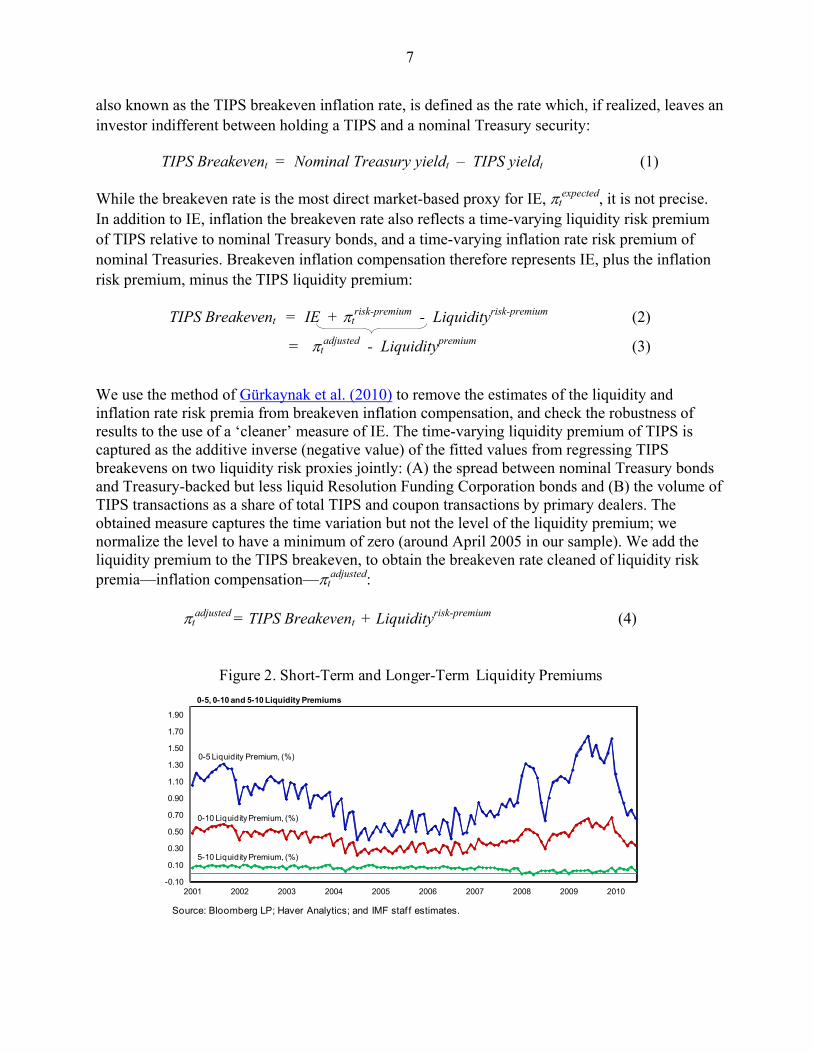
We use the method of Gürkaynak et al. (2010) to remove the estimates of the liquidity and inflation rate risk premia from breakeven inflation compensation, and check the robustness of results to the use of a ‘cleaner’ measure of IE. The time-varying liquidity premium of TIPS is captured as the additive inverse (negative value) of the fitted values from regressing TIPS breakevens on two liquidity risk proxies jointly: (A) the spread between nominal Treasury bonds and Treasury-backed but less liquid Resolution Funding Corporation bonds and (B) the volume of TIPS transactions as a share of total TIPS and coupon transactions by primary dealers. The obtained measure captures the time variation but not the level of the liquidity premium; we normalize the level to have a minimum of zero (around April 2005 in our sample). We add the liquidity premium to the TIPS breakeven, to obtain the breakeven rate cleaned of liquidity risk premia—inflation compensation—t

adjusted:

tadjusted = TIPS Breakevent + Liquidityrisk-premium (4)

Figure 2. Short-Term and Longer-Term Liquidity Premiums

-0.10

0.10

0.30

0.50

0.70

0.90

1.10

1.30

1.50

1.70

1.90

2001 2002 2003 2004 2005 2006 2007 2008 2009 2010

0-5, 0-10 and 5-10 Liquidity Premiums

5-10 Liquidity Premium, (%)




8

Second, to remove the estimate of the inflation rate risk from inflation compensation, tadjusted,

we use the Kalman filter procedure of Gürkaynak et al. (2010) (detailed in the Appendix). The Kalman filter smoothes t

adjusted around biannual yearly professional forecasters’ survey releases, which are taken as a correct (but possibly noisy) measure of actual IE, to obtain the final measure of ‘clean’ IE:

texpected = t

adjusted – trisk-premium (5)

The professional forecasters’ survey data on long-term inflation compensation used in Kalman filter has a drawback: it is only biennial and possibly overly stable over time. Therefore, the estimates of t

expected may underestimate the amount of variance in true IE; accordingly we treat them with caveats, as an illustrative measure.

Interest rates. We use five year nominal Treasury rates, five-to-ten year Treasury forward rates, and one-, two- and one-to-two Federal Funds futures rates.

Commodity prices. For crude oil prices, we use the average of West Texas Intermediate (WTI) and Brent indices,3 and focus on one-year ahead futures prices. For food prices, we construct a price index of one-year ahead futures contracts on representative agricultural commodities from the United Nations COMTRADE4 database, weighted by the global trade basket (detailed in Table A of the Appendix). In all exercises, we use the daily price changes in percent.

Macroeconomic controls. Controlling for macroeconomic variables helps isolate the impact of commodity prices from other macroeconomic shocks. We construct a daily dataset of surprise components of macroeconomic news using consensus forecasts and releases from Bloomberg. Following Gürkaynak et al. (2005), the surprise component of a release is defined as zero in dates with no release, and as the deviation between the released and the day-before consensus forecast of the macroeconomic variable upon a release. The surprises are taken in basis points and normalized by standard deviations to ensure comparability. We start with 70 release categories and, at first stage, run a stepwise regression to establish those with a significant effect on inflation compensation and interest rates. We then drop the releases that were not significant to arrive to a final list of 12 release categories detailed in Table B of the Appendix.

We also construct a daily dataset of changes in the nominal effective exchange rate (NEER) and in the VIX index using data from Haver Analytics and Bloomberg. Controlling for the NEER in our regressions ensures that we do not capture the effects of a monetary-policy induced change in the U.S. dollar exchange rate on the U.S. dollar prices of commodities as a pure commodity price shock, but rather as an exchange rate shock. Including the VIX in the regressions helps to control for global sentiment. 3 WTI is the benchmark price in the U.S.; Brent is a comparable London benchmark. While the oil market is efficient in the medium term, prices routinely deviate in the short-run due to transportation costs and other reasons such as storage bottlenecks (Borenstein et al., 1997).

4 For more information on how these weights are calculated, please see: unstats.un.org/unsd/tradekb/Attachment67 .aspx.

9

Survey-based inflation expectations. We use the mean, range and variance of 5–10 year-ahead IE from the monthly University of Michigan Survey of Consumers, from 2000 to 2011.

C. Empirical Strategy

Market-based IE and interest rates

For market-based data, we regress daily changes in near-term (0-5 year) and longer-term (5–10 year) IE and interest rate forwards on daily changes on oil and food prices, controlling for the surprise component of macroeconomic news releases, for changes to the nominal effective exchange rate, and VIX as a proxy for overall economic uncertainty. The controls allow isolating the impact of commodity prices from, for example, changes in medium-term aggregate demand outlook. The regressions are of the form:

∆Yt = α0 + λ*∆Oilt + θ*∆Foodt + i*MacroNewsi,t + *∆MacroControlst + Ɛt (1)

where ΔYt is the first difference in the measure of IE or interest rates, ΔFoodt is the percentage increase in the food index, and ΔOilt is the percentage increase in the oil prices as described in the previous section, MacroNewsi.t is the standardized surprise component of a macroeconomic announcement of type i and day t, and ΔMacroControlst is a set of macroeconomic controls consisting of changes in the U.S. nominal effective exchange rate, and changes in VIX.

We estimated equation (1) for TIPS breakeven yields, nominal Treasury yields, and the Federal Fund futures yields.

Survey-based IE

For survey data, we considered the following regressions using monthly observations:

∆Meant = α0 + λ*∆Oilt + θ*∆Foodt + Ɛt (2)

∆Variancet = α0 + λ* abs (∆Oilt ) + θ*abs (∆Foodt ) + Ɛt (3)

where ΔMeant is the difference in the mean survey-based IE, and ΔVariancet is the difference of the dispersion of University of Michigan long-term IE, ΔFoodt is the percentage increase in the food index, and ΔOilt is the percentage increase in crude oil prices. For the variance estimation, we use absolute changes of oil and food prices, because it is the magnitude and not necessarily the sign of the shock that should affect the dispersion of IE. We control for the year-on-year change in the seasonally adjusted CPI, for the unemployment rate, and for the first lag of the dependent variable.

10

III. RESULTS

A. Commodity Prices and TIPS-based IE

We first examine the effect of commodity price shocks on breakeven inflation rates. We regress daily changes in 0–5 and 5–10 years breakeven rates on oil and food price shocks, macroeconomic news surprises, and changes in the NEER and the VIX index. For oil price shocks, we use the percent change in the price of one-year ahead futures contracts. The results are similar using spot prices. The sample runs from January 2003 to April 2011, but excludes the crisis period of September 2008 to March 2009 that saw abnormally large fluctuations in the relative liquidity and yields of TIPS and nominal Treasury bonds.

Columns 1 and 2 of Table 1 report the results for the 0–5 and 5–10 year breakevens, respectively. Both oil and food price changes have statistically significant but modest effects on 0–5 year breakeven rates, consistent with the pass-through of commodity prices into consumer price inflation (column 1). A one percent increase in the oil price adds 0.70 basis point to the 0–5 year breakeven rate, whereas a one percent increase in the food price index adds 0.13 basis point. In addition, oil price shocks have an impact on longer-term inflation breakeven rates (column 2). A one percent increase in the price of oil adds 0.24 basis point to the 5–10 year breakeven rate.5

The estimated impact of oil price changes on breakeven inflation rates is economically significant. During the sustained commodity price rally from June 2010 to April 2011, short-term breakevens rose by 1.40 percentage points.6 Based on our estimates, 0.33 to 0.40 percentage point of this can be attributed to a 60 percent rise in oil prices, and another 0.05 percentage point to a 40 percent rise in the food prices. Thus, commodity prices could explain up to a third of the total increase in short-term inflation breakevens in that period. For longer-term breakeven inflation compensation, the 60 percent increase in commodity prices can explain about 0.20 percentage point – approximately a fifth of the 0.94 percentage point increase.

Columns 3 and 4 of Table 1 report results with the measures of inflation compensation (the breakeven rate ‘cleaned’ of liquidity risk premia), t

adjusted. The coefficients on oil futures price changes remains significant and are almost unchanged (the differences are not statistically different), confirming that TIPS liquidity risk is largely unaffected by commodity price shocks. A one percent increase in the price of oil futures adds about 0.65 basis point to 0–5 year inflation compensation and 0.23 basis point to 5–10 year inflation compensation.

5 The results are quantitatively similar to those of Beechey et al. (2011), who find that in 2003–07 a one percent increase in the oil price added 0.16 basis point to long-term IE.

6 Some commentators have attributed part of the increase in commodity prices during that period to the quantitative easing policy of the Federal Reserve (Reinhart (2011)).

11

Columns 5 and 6 report results with the measures of inflation compensation ‘cleaned’ also of inflation risk, t

expected. These estimates, while theoretically the closest to the ‘true’ IE, may underestimate the amount of variance in IE due to the imperfections of the Kalman filter procedure, which uses data on inflation expectations obtained from professional forecasters’ surveys, and such data are infrequent and possibly overly stable over time. Still, the coefficients are statistically significant and the signs remain robust, suggesting that we cannot attribute the impact of oil price shocks on inflation compensation solely to changes in inflation rate risk.

(1) (2) (3) (4) (5) (6)Dependent Variable 0-5 IE 5-10 IE 0-5 IE Cleaned of

Liquidity Risk5-10 IE Cleaned of Liquidity Risk

0-5 IE Cleaned of Liquidity and Inflation Rate Risk


Oil Futures Price Growth, % 0.702*** 0.240*** 0.657*** 0.233*** 0.058*** 0.151***

[0.052] [0.060] [0.102] [0.062] [0.009] [0.024]

Food Index Growth, % 0.132** 0.066 0.196* 0.059 0.023** 0.029

[0.060] [0.069] [0.118] [0.072] [0.010] [0.028]

Observations 2083 2083 2083 2083 2083 2083

R-squared 0.158 0.042 0.083 0.032 0.08 0.065

Sources: Bloomberg, LP; Haver Analytics; and Fund staff estimates.

Table 1. The Sensitivity of TIPS-based Noncleaned Inflation Compensation to Oil and Food Commodity Price Shocks

Notes: Standard errors are show n in brackets: *** p<0.01, ** p<0.05, * p<0.10. Ordinary least squares estimation on daily data. The dependent variable is the daily difference in inf lation compensation in basis points. Oil and food price grow th rates are expressed in percentages, and calculated by the formula (F'-F)/F, w here F and F' denote the price of the futures contract on tw o consecutive trading days. All regressions control for surprise components of macroeconomic new s releases: capacity utilization, CPI excluding food and energy, changes in nonfarm payrolls, current account, FOMC interest rate decisions, home sales, initial jobless claims, the ISM non-manufacturing survey, monthly budget, personal consumption, retail sales ex autos, for changes in the nominal exchange rate, and for the unemployment rate. We also control for VIX, as a measure of overall market uncertainty.

2000M1 - 2011M4 (excluding 2008M9 - 2009M3)

We next examine how our results differ between pre- and post-crisis subsamples. Our results for the pre-crisis sample (Table 1A) are comparable to those for the overall sample. The results for the post-crisis period (Table 2B) are based on a smaller subsample, but are nevertheless striking. The response of both 0–5 and 5–10 year breakeven rates to oil price shocks is much stronger than in the overall or the pre-crisis sample (columns 1 and 2 in Tables 1B versus the same columns in Table 1A). Based on the estimates in Table 1B, up to 40 percent of the increase in short-term and up to 20 percent of increase in long-term inflation expectations can be attributed to increased commodity prices (as compared to about 30 and 10 percent, respectively, based on the overall sample). The same result holds for the ‘cleaned’ IE measures—their sensitivity to oil price shocks is higher in the post-crisis sample than in the pre-crisis sample, for both the longer-term and short-term horizons (columns 3–6 in Table 1A as compared to the same columns in Table 1B).

The increased sensitivity of 0–5 inflation compensation to oil price shocks post- crisis appears to reflect in large part a higher inflation risk premium, whereas the increased sensitivity of 5–10 compensation seems to reflect the higher sensitivity of IE to oil price shocks.

In the post crisis sample, removing the inflation risk premium makes a substantial difference for the estimated effect oil price shocks on 0-5 compensation in columns 3 and 5 of Table 1B. Interestingly, the impact of correcting for inflation rate risk is smaller for 5–10 inflation compensation, suggesting—plausibly—that the heightened effect of oil price shocks on inflation rate risk post-crisis was primarily present at shorter horizons (the results should be interpreted with caution given the excess smoothing of the Kalman filter procedure). The increase in the sensitivity of 5–10 inflation compensation to oil shocks post-crisis is similar for all three

12

measures of inflation compensation, suggesting a role for not only increased inflation rate risk, but also an increased impact on the level of IE.






[0.054] [0.060] [0.091] [0.061] [0.008] [0.023]

Food Index Growth, % 0.171*** 0.076 0.198* 0.08 0.022** 0.028

[0.064] [0.072] [0.109] [0.072] [0.010] [0.028]

Observations 1717 1717 1717 1717 1717 1717

R-squared 0.145 0.032 0.07 0.031 0.062 0.057


Table 1A. The Sensitivity of TIPS-based Noncleaned Inflation Compensation to Oil and Food Commodity Price Shocks Pre-Crisis

2000M1 - 2008M8 (Pre-crisis)

Notes: Standard errors are show n in brackets: *** p<0.01, ** p<0.05, * p<0.10. Ordinary least squares estimation on daily data. The dependent variable is the daily difference in inf lation compensation 'cleaned' of liquidity risk in basis points. Oil and food price grow th rates are expressed in percentages, and calculated by the formula (F'-F)/F, w here F and F' denote the price of the futures contract on tw o consecutive trading days. All regressions control for surprise components of macroeconomic new s releases: capacity utilization, CPI excluding food and energy, changes in nonfarm payrolls, current account, FOMC interest rate decisions, home sales, initial jobless claims, the ISM non-manufacturing survey, monthly budget, personal consumption, retail sales ex autos, for changes in the nominal exchange rate, and for the unemployment rate. We also control for VIX, as a measure of overall market uncertainty.





Oil Futures Price Growth, % 0.850*** 0.404** 0.840** 0.294* 0.066** 0.236***

[0.152] [0.185] [0.410] [0.139] [0.033] [0.082]

Food Index Growth, % -0.017 -0.049 0.186 -0.087 0.024 0.011

[0.152] [0.185] [0.411] [0.220] [0.033] [0.082]

Observations 364 364 364 364 364 364

R-squared 0.26 0.157 0.125 0.072 0.139 0.143


2009M4 - 2011M4 (Post-crisis)

Notes: Standard errors are show n in brackets: *** p<0.01, ** p<0.05, * p<0.10. Ordinary least squares estimation on daily data. The dependent variable is the daily difference in inf lation compensation cleaned of the liquidity and inflation risk premiums, in basis points. Oil and food price grow th rates are expressed in percentages, and calculated by the formula (F'-F)/F, w here F and F' denote the price of the futures contract on tw o consecutive trading days. All regressions control for surprise components of macroeconomic new s releases: capacity utilization, CPI excluding food and energy, changes in nonfarm payrolls, current account, FOMC interest rate decisions, home sales, initial jobless claims, the ISM non-manufacturing survey, monthly budget, personal consumption, retail sales ex autos, for changes in the nominal exchange rate, and for the unemployment rate. We also control for VIX, as a measure of overall market uncertainty.

Table 1B. The Sensitivity of TIPS-based Noncleaned Inflation Compensation to Oil and Food Commodity Price Shocks Post-Crisis

Could longer-term inflation expectations react to near-term oil price movements because agents expect a sustained rally in commodity prices when they observe increases in near-term oil prices? We test this hypothesis by regressing the changes in far-ahead expected oil prices on changes in one-year ahead prices (Table F in the appendix). We find that a given percentage change in the one-year ahead oil-price tends to coincide with a smaller percentage increase in prices for farther-ahead contracts. Thus, we don’t find evidence in support of this potential explanation.

To summarize, longer-term inflation breakevens could respond to oil price shocks either because oil price shocks have a genuine impact on expected long-term core IE, or because oil price shocks increase perceptions of inflation rate risk by fueling uncertainty about how aggregate demand and monetary policy will respond to oil price movements. Our results suggest that some effect on core IE cannot be dismissed using available tools for estimating inflation rate risk (significant

13

coefficients in column 6 of Tables 1, 1A, 1B). But we also have no reason to discard the inflation rate risk effect—and this channel gets additional validation from survey-based data in the next section. Overall, our assessment is that both effects are likely at play, and may have become stronger after the crisis.

B. Commodity Prices and Survey-Based IE

We next examine consumer IE in the Reuters/University of Michigan Survey of Consumers. Survey predictions of IE are available at a monthly frequency, in contrast to the daily market-based measures.

Using a consumer survey rather than a survey of professional forecasters to gauge longer-term IE has pros and cons. Both measures are imperfect. Professional forecasters’ expectations are not responsive enough because of difficulties in formally forecasting long-term inflation—it’s hard to justify an assumption different from the implicit Fed target. On the other hand, consumer forecasts are subject to behavioral biases that may give increased weight to the more volatile, non-core components of prices, such as food and gasoline (Van der Klaauw et al., (2008), Bruine de Bruin et al., (2011), and Armantier et al., (2011)). Despite this limitation, looking at consumer forecasts is helpful since households’ perceptions, even when biased, can affect wage pressures and as a consequence, actual inflation.

We regress changes in the mean and variance of longer term (for the next 5 to 10 years) IE in the Reuters/University of Michigan Survey on changes in oil and commodity food prices, controlling for the unemployment rate and the year-on-year inflation rate observed in the current month, as well as the first lag of the dependent variable. We use the growth rate of oil and food prices for explaining the change in the mean of expected inflation, and the absolute value of the change in oil and food prices for explaining the change in the variance, since both declines and increases in oil prices could raise inflation uncertainty. We investigate the 2000M1–2011M4 period, looking at full sample as well as the pre-crisis subsample (the post-crisis subsample is too short to draw inference).

We find that oil price shocks affect the variance of expected inflation among survey respondents, but only when the post-crisis period is included. Although the mean of expected inflation increases with oil and food price rises, the coefficients are not statistically significant. These findings suggest that oil price shocks had an effect on consumers’ perceived inflation rate risk, primarily in the post-crisis period.

14

(1) (2) (3) (4)

Dependent Variable ∆ mean ∆ variance ∆ mean ∆ variance

Oil Futures Price Growth, % 0.335 8.707* 0.098 -1.503

[0.301] [4.471] [0.367] [4.706]

Food Index Growth, % 0.208 5.255 0.453 0.862

[0.300] [4.226] [0.360] [4.393]

Observations 134 134 104 104

R-squared 0.294 0.106 0.364 0.249

Sources: Bloomberg, LP; Thompson Reuters / University of Michigan Survey of Consumers; and FRED St. Louis.

2000M1 - 2011M4 2000M1 -2008M8 (Pre-crisis)

Table 2. The Sensitivity of Survey-Based 5-10 IE to Oil and Food Commodity Price Shocks

Notes: Standard errors are show n in brackets: *** p<0.01, ** p<0.05, * p<0.10. Ordinary least squares estimation on monthly data. The dependent variable is the monthly difference in the mean and variance of survey-based IE. Oil and food price grow th rates are expressed in percentages, and calculated by the formula (F'-F)/F, w here F and F' denote the mean price of the futures contract on tw o consecutive trading months. For the variance estimations, w e use the food and oil price shocks in absolute terms because it is the magnitude of the shock and not the sign of it that should affect dispersion measures of inflation expectations. We control for the year-on-year change in the seasonally adjusted CPI, for the unemployment rate, and for the first lag of the dependent variable.

C. Commodity Prices and Interest Rates

How does the stronger sensitivity of inflation compensation to oil price shocks in the post-crisis period relate to monetary policy expectations? In this section, we analyze the effects of commodity prices on nominal interest rates (nominal Treasury forwards and Federal Funds futures), which capture market participants’ anticipation of the future monetary policy stance.

The results for forward nominal rates are shown in Table 3 and those for Federal Funds futures in Table 4. The results in columns 3 and 4 of Table 3 and columns 4–6 of Table 4 show that, prior to the crisis (during 2003Q1–2008Q3), commodity price shocks did not affect nominal interest rates: markets did not expect the Fed to react to commodity price changes in a systematic way. This is consistent with the notion that commodity price shocks raise headline inflation, but lower aggregate demand (with expected output declining relative to potential output), leading to an overall insignificant net effect in the pre-crisis period.

In contrast, since the crisis period, oil prices are positively related to nominal interest rates (columns 5–6 in Table 3 and columns 7–9 in Table 4). A possible explanation could be that, during the post-crisis recovery, oil price increases were seen by market participants as indicators of economic recovery, reinforcing expectations that commodity price increases would be met by a relatively faster exit from extraordinarily low interest rates.

15

(1) (2) (3) (4) (5) (6)

Dependent Variable 0-5 Nominal Rates

5-10 Nominal Rates

0-5 Nominal Rates

5-10 Nominal Rates

0-5 Nominal Rates

5-10 Nominal Rates

Oil Futures Price Growth, % 0.279*** 0.324*** 0.126 0.110 0.752*** 0.870***

[0.081] [0.086] [0.087] [0.083] [0.224] [0.315]

Food Index Growth, % 0.194** 0.115 0.105 0.015 0.159 0.094

[0.097] [0.102] [0.108] [0.104] [0.214] [0.301]

Observations 2557 2557 2075 2075 480 480

R-squared 0.131 0.045 0.145 0.039 0.239 0.14


Notes: Standard errors are show n in brackets: *** p<0.01, ** p<0.05, * p<0.10. Ordinary least squares estimation on daily data. The dependent variable is the daily dif ference in nominal forw ard rates in basis points. Oil and food price grow th rates are expressed in percentages, and calculated by the formula (F'-F)/F, w here F and F' denote the price of the futures contract on tw o consecutive trading days. All regressions control for surprise components of macroeconomic new s releases: capacity utilization, CPI excluding food and energy, changes in nonfarm payrolls, current account, FOMC interest rate decisions, home sales, initial jobless claims, the ISM non-manufacturing survey, monthly budget, personal consumption, retail sales ex autos, changes to the nominal exchange rate and changes in the unemployment rate. We also control for VIX, as a measure of overall market uncertainty.

Table 3. The Sensitivity of Nominal Forward Rates to Oil and Food Commodity Price Shocks

2000M1 -2011M4 (excluding 2008M9-2009M3)

2000M1 -2008M8 (pre-crisis)

2009M4 -2011M4 (post-crisis)

(1) (2) (3) (4) (5) (6) (7) (8) (9)

Dependent Variable 0-1 Fed Funds Rates

0-2 Fed Funds Rates

1-2 Fed Funds Rates

0-1 Fed Funds Rates

0-2 Fed Funds Rates

1-2 Fed Funds Rates

0-1 Fed Funds Rates

0-2 Fed Funds Rates

1-2 Fed Funds Rates

Oil Futures Price Growth, % 0.482* 0.303** 0.546*** 0.425 0.113 0.138 0.441** 0.776*** 1.326**

[0.427] [0.119] [0.199] [0.534] [0.134] [0.191] [0.186] [0.272] [0.594]

Food Index Growth, % 0.117 0.201 0.327 -0.018 0.186 0.293 0.126 0.177 0.24

[0.495] [0.137] [0.230] [0.645] [0.164] [0.234] [0.178] [0.260] [0.567]

Observations 1736 1416 1413 1370 1051 1048 364 364 364

R-squared 0.009 0.144 0.095 0.013 0.116 0.069 0.298 0.27 0.193


2000M1 -2011M4 (excluding 2008M9-2009M3)

2000M1 -2008M8 (pre-crisis)

2009M4 -2011M4 (post-crisis)

Table 4. The Sensitivity of Federal Fund Forward Rates to Oil and Food Commodity Price Shocks

Notes: Standard errors are show n in brackets: *** p<0.01, ** p<0.05, * p<0.10. Ordinary least squares estimation on daily data. The dependent variable is the daily dif ference in the Fed Fund forw ard rates in basis points. Oil and food price grow th rates are expressed in percentages, and calculated by the formula (F'-F)/F, w here F and F' denote the price of the futures contract on tw o consecutive trading days. All regressions control for surprise components of macroeconomic new s releases: capacity utilization, CPI excluding food and energy, changes in nonfarm payrolls, current account, FOMC interest rate decisions, home sales, initial jobless claims, the ISM non-manufacturing survey, monthly budget, personal consumption, retail sales ex autos, changes to the nominal exchange rate and changes in the unemployment rate. We also control for VIX, as a measure of overall market uncertainty.

16

IV. CONCLUSIONS

We examined the sensitivity of U.S. inflation compensation to commodity price shocks before and after the 2008–09 financial crisis, using market- and survey-based data. We find that oil and food price shocks have a significant impact on short-term inflation compensation embedded in U.S. Treasury bonds, consistent with the pass-through of commodity price shocks to headline inflation. More surprisingly, oil price shocks also have a statistically significant, albeit economically small, impact on longer-term inflation compensation. Both short- and long-term inflation compensation have become more responsive to oil price shocks since the crisis, possibly due to increased inflation uncertainty, especially in the shorter term.

The higher sensitivity of short-term inflation compensation to oil prices since the crisis is not attributable to expectations of a weaker monetary policy response relative to the pre-crisis period—our results in fact suggest that oil price shocks raised near-term expectations of federal fund rates more strongly in the post-crisis period. It thus appears more likely that on average markets associated oil price increases with a stronger U.S. economic recovery in the aftermath of the Great Recession, thereby raising their expectations of inflation and policy interest rates simultaneously.

The sensitivity of long-term inflation compensation to commodity price shocks is consistent with their impact either on inflation expectation or on perceived inflation rate risk. We are not able to dismiss any of the two channels. Illustrative exercises based on correcting for inflation rate risk in the measures of inflation compensation, and on assessing the impact of oil price shocks on inflation expectations elicited from consumer surveys suggest that both effects are likely at play. The effects on commodity price shocks on inflation expectations are economically modest. Yet the fact that the relationship between oil prices and inflation expectations is statistically significant and seems to have become stronger after the crisis calls for continued vigilance.

17

APPENDIX

Table A. Weights for Calculating the IMF Food Price Index

Commodity Weights Obs Mean Std. Dev. Min Max

Barley 0.254 2088 137.55 42.22 79.81 267.55

Corn 1.042 2088 3.86 1.35 2.28 8.34

No. 11 World Sugar 0.606 683 0.18 0.04 0.12 0.30

No. 14 US Sugar 0.053 347 0.31 0.04 0.25 0.39

Palm oil 0.712 2088 611.17 252.08 331.58 1343.67

Poultry 0.877 2088 0.78 0.08 0.62 0.89

Rice 0.638 2088 10.79 3.75 3.94 24.46

Soybean meal 0.841 2088 253.00 72.21 147.00 453.90

Soybean Oil 0.429 2088 0.34 0.12 0.19 0.70

Soybeans 1.219 2088 8.65 2.73 5.00 16.58

Swine 1.143 2088 65.00 10.48 0.00 93.87

Wheat 1.655 2088 5.82 1.95 3.37 13.78

Food Index n.a. 2088 715.06 249.80 403.87 1391.45

Source: IMF; Bloomberg LP; and IMF staff estimates.

Table B. Standardized Macroeconomic News Surprises

Macroeconomic News Obs Mean Std. Dev. Min Max

2163 -0.005 0.212 -4.528 2.113

2163 -0.002 0.197 -2.040 3.061

2163 -0.002 0.229 -3.130 4.935

2163 0.002 0.124 -2.552 2.057

2163 -0.003 0.118 -3.670 1.761

2163 0.006 0.197 -3.417 1.750

2163 0.014 0.463 -4.701 3.172

2163 0.004 0.179 -3.603 2.305

2163 -0.001 0.130 -2.470 2.171

2163 0.003 0.205 -2.925 3.803

2163 0.001 0.209 -3.379 2.782

2163 -0.006 0.200 -3.140 2.512

Source: Bloomberg LP; and IMF staff estimates.

Unemployment rate

Notes: The surprise component of a release is defined as zero in dates w ith no release, and as the deviation betw een the released and the day-before consensus forecast of the macroeconomic variable if there is a release. The releases are taken in basis points and normalized by standard deviations to assure comparability. One reason is that measurement units can be different, for example changes in GDP are often calculated as percentages, w hereas payrolls are measured in thousands of jobs. In addition scaling is often different, thus for example year-on-year changes are likely to be larger than month-on-month f igures.

Personal Consumption

Retail Sales ex auto

Capacity utilization

CPI ex food and energy

Change in Non-farm

Current account

FOMC

Home Sales

Initial jobless claims

ISM non-manufacturing

Monthly budget

18

(1) (2) (3) (4) (5) (6)

Dependent Variable 0-5 IE 5-10 IE 0-5 IE Cleaned of Liquidity Risk

5-10 IE Cleaned of Liquidity Risk



Capacity Utilization 0.008** 0.006 0.001 0.007 0.000 0.001

[0.004] [0.005] [0.008] [0.005] [0.001] [0.002]

CPI excluding Food & Energy 0.019*** 0.007 0.034*** 0.008* 0.003*** 0.006***

[0.004] [0.005] [0.008] [0.005] [0.001] [0.002]

∆ Nonfarm Payroll 0.015*** 0.000 0.042*** -0.010** 0.003*** 0.005***

[0.004] [0.004] [0.007] [0.004] [0.001] [0.002]

Current Account 0.001 -0.003 -0.021* 0.004 -0.001 -0.001

[0.006] [0.007] [0.011] [0.007] [0.001] [0.003]

FOMC -0.006 -0.020** 0.007 -0.027*** 0.000 -0.005

[0.009] [0.010] [0.017] [0.010] [0.001] [0.004]

Home Sales 0.005 0.004 0.009 0.003 0.001** 0.001

[0.004] [0.004] [0.007] [0.004] [0.001] [0.002]

Initial Jobless Claims -0.003* -0.004** -0.006* -0.004* 0.000 -0.001*

[0.002] [0.002] [0.003] [0.002] [0.000] [0.001]

ISM Non-Manufacturing Index 0.002 -0.001 -0.003 0.000 0.000 -0.001

[0.004] [0.005] [0.008] [0.005] [0.001] [0.002]

Monthly Budget Statement -0.005 -0.003 -0.008 -0.004 -0.001 -0.002

[0.003] [0.004] [0.007] [0.004] [0.001] [0.002]

Personal Consumption 0.005 0.012*** 0.017** 0.008* 0.001* 0.005***

[0.004] [0.004] [0.008] [0.005] [0.001] [0.002]

Retail Sales Excluding Auto 0.008** 0.007* 0.014** 0.006 0.001** 0.004**

[0.004] [0.004] [0.007] [0.004] [0.001] [0.002]

∆ Effective exchange rate -0.001 -0.002 -0.008 0.000 -0.001* 0.000

[0.004] [0.004] [0.007] [0.004] [0.001] [0.002]

∆ Unemployment Rate -0.229 0.288 -1.103* 0.761** -0.075 0.000

[0.289] [0.330] [0.567] [0.347] [0.049] [0.133]

∆ Vix Index -0.104*** -0.087*** -0.142*** -0.064*** -0.011*** -0.037***

[0.013] [0.014] [0.025] [0.015] [0.002] [0.006]


[0.052] [0.060] [0.102] [0.062] [0.009] [0.024]

Food Index Growth, % 0.132** 0.066 0.196* 0.059 0.023** 0.029

[0.060] [0.069] [0.118] [0.072] [0.010] [0.028]

Observations 2083 2083 2083 2083 2083 2083

R-squared 0.158 0.042 0.083 0.032 0.080 0.065


Table C. The Sensitivity of TIPS-based Inflation Compensation to Oil and Food Commodity Price Shocks

2001M7 - 2011M4 (excluding 2008M9 - 2009M3)

Notes: Standard errors are show n in brackets: *** p<0.01, ** p<0.05, * p<0.10. Ordinary least squares estimation on daily data. The dependent variable is the daily dif ference in inf lation expectations in basis points. Oil and food price grow th rates are expressed in percentages, and calculated by the formula (F'-F)/F, w here F and F' denote the price of the futures contract on tw o consecutive trading days. All regressions control for surprise components of macroeconomic new s releases: capacity utilization, CPI excluding food and energy, changes in nonfarm payrolls, current account, FOMC interest rate decisions, home sales, initial jobless claims, the ISM non-manufacturing survey, monthly budget, personal consumption, retail sales ex autos. We also control for daily changes in the nominal effective exchange rate, for the unemployment rate, and for VIX, as a measure of overall market uncertainty.

19

(1) (2) (3) (4) (5) (6)





Capacity Utilization 0.007* 0.008* 0.004 0.007 0.000 0.002

[0.004] [0.005] [0.007] [0.005] [0.001] [0.002]

CPI excluding Food & Energy 0.017*** 0.008* 0.034*** 0.009* 0.003*** 0.007***

[0.004] [0.005] [0.007] [0.005] [0.001] [0.002]

∆ Nonfarm Payroll 6.459*** 2.585 8.447*** 2.426 0.652*** 2.242***

[1.578] [1.762] [2.661] [1.771] [0.243] [0.680]

Current Account -0.008 0.001 -0.019* 0.002 -0.001 -0.002

[0.007] [0.008] [0.012] [0.008] [0.001] [0.003]

FOMC -0.006 -0.016 0.001 -0.016 0.000 -0.003

[0.009] [0.010] [0.015] [0.010] [0.001] [0.004]

Home Sales 0.001 0.000 -0.002 0.000 0.000 -0.001

[0.004] [0.005] [0.007] [0.005] [0.001] [0.002]

Initial Jobless Claims -0.004** -0.002 -0.004 -0.002 0.000 -0.001

[0.002] [0.002] [0.003] [0.002] [0.000] [0.001]

ISM Non-Manufacturing Index 0.003 0.000 -0.001 0.000 0.000 0.000

[0.004] [0.004] [0.007] [0.004] [0.001] [0.002]

Monthly Budget Statement -0.007** -0.003 -0.008 -0.003 -0.001* -0.002

[0.003] [0.004] [0.006] [0.004] [0.001] [0.001]

Personal Consumption 0.005 0.014*** 0.012 0.013** 0.001 0.006***

[0.005] [0.005] [0.008] [0.005] [0.001] [0.002]

Retail Sales Excluding Auto 0.005 0.002 0.008 0.002 0.001 0.002

[0.004] [0.004] [0.006] [0.004] [0.001] [0.002]

∆ Effective exchange rate 0.247 1.152*** -0.164 1.142*** -0.002 0.273**

[0.320] [0.357] [0.539] [0.359] [0.049] [0.138]

∆ Unemployment Rate -0.006 -0.004 -0.009 -0.003 -0.001** -0.001

[0.004] [0.004] [0.006] [0.004] [0.001] [0.002]

∆ Vix Index -0.092*** -0.052*** -0.107*** -0.048*** -0.008*** -0.027***

[0.013] [0.015] [0.023] [0.015] [0.002] [0.006]


[0.054] [0.060] [0.091] [0.061] [0.008] [0.023]

Food Index Growth, % 0.171*** 0.076 0.198* 0.080 0.022** 0.028

[0.064] [0.072] [0.109] [0.072] [0.010] [0.028]

Observations 1717 1717 1717 1717 1717 1717

R-squared 0.145 0.032 0.070 0.031 0.062 0.057


Table D. The Sensitivity of TIPS-based Inflation Compensation to Oil and Food Commodity Price Shocks Pre-Crisis

2001M7 - 2008M8

Notes: Standard errors are show n in brackets: *** p<0.01, ** p<0.05, * p<0.10. Ordinary least squares estimation on daily data. The dependent variable is the daily difference in inflation expectations in basis points. Oil and food price grow th rates are expressed in percentages, and calculated by the formula (F'-F)/F, w here F and F' denote the price of the futures contract on tw o consecutive trading days. All regressions control for surprise components of macroeconomic new s releases: capacity utilization, CPI excluding food and energy, changes in nonfarm payrolls, current account, FOMC interest rate decisions, home sales, initial jobless claims, the ISM non-manufacturing survey, monthly budget, personal consumption, retail sales ex autos. We also control for daily changes in the nominal effective exchange rate, for the unemployment rate, and for VIX, as a measure of overall market uncertainty.

20

(1) (2) (3) (4) (5) (6)





Capacity Utilization 0.013 -0.008 -0.014 0.000 -0.001 -0.004

[0.012] [0.015] [0.032] [0.017] [0.003] [0.006]

CPI excluding Food & Energy 0.027** 0.004 0.035 0.006 0.003 0.004

[0.011] [0.013] [0.028] [0.015] [0.002] [0.006]

∆ Nonfarm Payroll 0.014*** 0.000 0.042*** -0.010 0.003*** 0.005**

[0.004] [0.005] [0.012] [0.006] [0.001] [0.002]

Current Account 0.020* -0.011 -0.025 0.007 -0.002 0.000

[0.012] [0.014] [0.032] [0.017] [0.003] [0.006]

FOMC -0.017 -0.087** 0.002 -0.119** 0.001 -0.024

[0.032] [0.039] [0.087] [0.047] [0.007] [0.017]

Home Sales 0.010 0.011 0.027 0.008 0.002 0.005

[0.007] [0.009] [0.019] [0.010] [0.002] [0.004]

Initial Jobless Claims 0.000 -0.011** -0.013 -0.009 -0.001 -0.004

[0.004] [0.005] [0.012] [0.006] [0.001] [0.002]

Monthly Budget Statement 0.015 -0.009 0.003 -0.009 0.000 -0.003

[0.014] [0.017] [0.037] [0.020] [0.003] [0.007]

Personal Consumption 0.009 0.025* 0.031 0.021 0.002 0.009

[0.010] [0.013] [0.028] [0.015] [0.002] [0.006]

Retail Sales Excluding Auto 0.021** 0.026** 0.034 0.020 0.003 0.009*

[0.009] [0.011] [0.025] [0.013] [0.002] [0.005]

∆ Effective exchange rate -0.001 0.001 -0.002 0.001 -0.000* -0.001

[0.001] [0.001] [0.002] [0.001] [0.000] [0.000]

∆ Unemployment Rate 0.012 0.004 -0.009 0.009 0.000 0.000

[0.009] [0.011] [0.025] [0.013] [0.002] [0.005]

∆ Vix Index -0.143*** -0.207*** -0.267*** -0.118** -0.022*** -0.066***

[0.037] [0.044] [0.098] [0.053] [0.008] [0.020]

Oil Futures Price Growth, % 0.850*** 0.404** 0.840** 0.294* 0.066** 0.236***

[0.152] [0.185] [0.410] [0.139] [0.033] [0.082]

Food Index Growth, % -0.017 -0.049 0.186 -0.087 0.024 0.011

[0.152] [0.185] [0.411] [0.220] [0.033] [0.082]

Observations 364 364 364 364 364 364

R-squared 0.260 0.157 0.125 0.072 0.139 0.143


Table E. The Sensitivity of TIPS-based Inflation Compensation to Oil and Food Commodity Price Shocks Post-Crisis

2009M4 - 2011M4

Notes: Standard errors are show n in brackets: *** p<0.01, ** p<0.05, * p<0.10. Ordinary least squares estimation on daily data. The dependent variable is the daily difference in inflation expectations in basis points. Oil and food price grow th rates are expressed in percentages, and calculated by the formula (F'-F)/F, w here F and F' denote the price of the futures contract on tw o consecutive trading days. All regressions control for surprise components of macroeconomic new s releases: capacity utilization, CPI excluding food and energy, changes in nonfarm payrolls, current account, FOMC interest rate decisions, home sales, initial jobless claims, the ISM non-manufacturing survey, monthly budget, personal consumption, retail sales ex autos. We also control for daily changes in the nominal effective exchange rate, for the unemployment rate, and for VIX, as a measure of overall market uncertainty.

21

(1) (2) (3) (4) (1) (2) (3) (4)

Dependent variable --> 2 years ahead

3 years ahead

4 years ahead

5 years ahead

2 years ahead

3 years ahead

4 years ahead

5 years ahead

0.874*** 0.829*** 0.820*** 0.798*** 0.941*** 0.873*** 0.816*** 0.649***

[0.011] [0.014] [0.016] [0.019] [0.005] [0.011] [0.021] [0.090]

Observations 716 716 716 647 655 459 262 64

R-squared 0.898 0.822 0.785 0.732 0.9845 0.9335 0.8491 0.4569

Sources: Authors' calculations based on oil price data obtained through Bloomberg and Haver Analytics.

Notes: Standard errors are show n in brackets: *** p<0.01, ** p<0.05, * p<0.10. Ordinary least squares estimation on daily data. OLS regressions of daily percentage changes in oil prices expected in 2, 3, 4, and 5 years on daily percentage changes in prices expected one year ahead and a constant. Standards errors are given in brackets.

Table F. Correlation Between Changes In Expected Oil Prices At Different Horizons

2000M1 - 2008M8 (Pre-Crisis)

Percent change in the price of oil, based on the one-year ahead future contract

2009M4 - 2011M4 (Post-Crisis)

22

The Gürkaynak et al. (2010) Kalman filter-based method for cleaning inflation compensation of inflation rate risk.

We use the Kalman filter-based procedure to estimate a state-space model by maximum likelihood, given bi-yearly professional survey releases and daily market-based IE containing inflation rate risk. The Kalman filter extracts the inflation risk premium, producing values that tend to be closer to the expected forward inflation. More precisely, we take the inflation compensation forward rates at either five or five-to-ten year horizons, adjusted by the liquidity premium as estimated previously, t

adjusted, and assume that this represents the sum of IE and the inflation risk premium:

tadjusted = t

expected + trisk-premium (1)

We also assume that the professional forecasts7 at the same five- and five-to-ten year horizons predict on average correct latent IE and can be expressed as noisy measures of these latter:

tsurvey = t

expected + utsurvey (2)

where utsurvey is independently and identically distributed ~ (0, σsurvey

2).

Equations (1) and (2) now give a measurement equation for a system in state space form where (t

expected , trisk-premium) is the state vector. The following transition equation assumes, by the model

of Stock and Watson (2007), that the long-run IE can be predicted by a random walk, while the inflation risk premium is an AR(1) process:

=

where and are mutually uncorrelated and iid ~ (0, σ12) and ~ (0, σ2

2) respectively. We set σ1

2 to an estimated average since 1999 from fitting the Stock and Watson model8 to actual CPI inflation data by the method detailed in Gürkaynak et al. (2010). The Kalman filter produces smoothed and cleaned IE.

7 We use bi-annual Blue Chip and Survey of Professional Forecasters inflation expectations.

8 See Stock and Watson (1999).

23

REFERENCES

Armantier, O., W. Bruine de Bruin, G. Topa, W. van der Klaauw, and B. Zafar, 2011,Inflation Expectations and Behavior: Do Survey Respondents Act on Their Beliefs? Federal Reserve Board of New York, Staff Report No. 509.

Beechey, M.J., B.K. Johannsen, and A.T. Levin, 2011, Are Long-Run IE Anchored More Firmly in the Euro Area Than in the United States? American Economic Journal: Macroeconomics, 3(2), 104–29. doi:10.1257/mac.3.2.104

__________, and J.H.Wright, 2009, The high-frequency impact of news on long-term yields and forward rates: Is it real? Journal of Monetary Economics, Elsevier, 56(4), 535–44. doi:10.1016/j.jmoneco.2009.03.011

Borenstein, S., C.A. Cameron, R. Gilbert, 1997, Do Gasoline Prices Respond Asymmetrically to Crude Oil Price Changes? The Quarterly Journal of Economics, 112(1), 305–39. doi:10.1162/003355397555118

Bruine de Bruin, W., C.F. Manski, G. Topa, and W. van der Klaauw, W., 2011, Measuring Consumer Uncertainty about Future Inflation. Journal of Applied Econometrics, 26(3), 454–78. doi: 10.1002/jae.1239

Clark, T. E., and T. Nakata, 2008, Has the Behavior of Inflation and Long-Term Inflation Expectations Changed? Economic Review, Federal Reserve Bank of Kansas City, 1(1), 17–50.

D’Amico, S., D.H. Kim, and M Wei, 2010, Tips From TIPS: The Informational Content of Treasury Inflation-Protected Security Prices. Federal Reserve Bank of Washington D.C., Staff Working Paper No. 19.

FOMC [Federal Open Markets Committee], March 2011, Press Release. Retrieved from http://www.federalreserve.gov/newsevents/press/monetary/20110315a.htm.

Gerlach, P., P. Hördahl, and R. Moessner, 2011, Inflation Expectations and the Great Recession. BIS Quarterly Review, 3(1).

Gürkaynak, R.S., B. Sack, and J.H.Wright, 2010, The TIPS Yield Curve and Inflation Compensation. American Economic Journal: Macroeconomics, 2(1), 70–92. doi:10.1257/mac.2.1.70

__________, and E. Swanson, 2005, The Sensitivity of Long-Term Interest Rates to Economic News: Evidence and Implications for Macroeconomic Models. American Economic Review, 95(1), 425–36. doi:10.1.1.178.5999

__________, A.T. Levin, A.N. Marder, and E.T. Swanson, E. T., 2007, Inflation Targeting and the Anchoring of Inflation Expectations in the Western Hemisphere. Economic Review, Federal Reserve Bank of San Francisco, 25–47.

24

Hamilton, J.D. (2008). Understanding Crude Oil Prices. The Quarterly Journal of the IAEE's Energy Economics Education Foundation, 30(2), 179–206. doi:10.5547/ISSN0195-6574-EJ-Vol30-No2–9

Simon, J., D. Leigh, A. Pescatori, A. Alichi, L. Catao, O. Kamenik, H. Kim, D. Laxton, R. Portillo, and F. Zanna, September 2011, Target What You Can Hit: Commodity Price Swings and Monetary Policy. International Monetary Fund, World Economic Outlook, Chapter 3 (Washington).

Kilian, L., 2008, The Economic Effects of Energy Price Shocks. Journal of Economic Literature, 46(4), 871–909. doi:10.1257/jel.46.4.871

Reinhart, V. R., 2011, Hearing on How Federal Reserve Policies Add to Hard Times at the Pump. Statement before the United States House of Representatives, American Enterprise Institute. Retrived from: http://www.cepr.net/index.php/events/events/how-federal-reserve-policies-add-to-hard-times-at-the-pump

Roache, S. K., and D.A.Reichsfeld, 2011, Do Commodity Futures Help Forecast Spot Prices? International Monetary Fund, Working Paper No. 11/254.

Sill, K., 2007, The Macroeconomics of Oil Shocks. Federal Reserve Bank of Philadelphia, Business Review, 1(1), 21–31.

Stock, J. H., and M. W. Watson, 1999, Forecasting Inflation. Journal of Monetary Economics, 44(2), 293–335.

____________, 2007, Has U.S. Inflation Become Harder to Forecast? Journal of Money, Credit, and Banking, 39, 3–33. doi=10.1.1.174.7404

Van der Klaauw, W., W. Bruine de Bruin, G. Topa, S. Potter, and M.F. Bryan, 2008, Rethinking the Measurement of Household Inflation Expectations: Preliminary Findings. Federal Reserve Bank of New York, Staff Report No. 359.

commodity prices and inflation expectations in the · pdf filecommodity prices and inflation...

Documents