from WORLD ECONOMIC OUTLOOK October 2013

Commodity Market Review

International Monetary Fund

1

SPECIAL FEATURE: COMMODITY MARKET REVIEW1

The impact of slowing emerging market growth is being felt on commodity prices, particularly metals. The first section of this special feature discusses likely first-round impacts of these declines on trade balances and the short run challenges from a more balanced and sustainable growth path in China for metal and energy exporters. It concludes with the price outlook and risks. The second section studies the impacts of the U.S. energy boom. Although the boom has disrupted relationships between some energy prices, impacts on U.S. output and the current account will be modest.

Recent Developments and Impact of Emerging Markets Slowdown

Metals prices have declined while energy and food prices have edged up. The IMF’s Primary Commodities Price Index is unchanged from March 2013, with declines in metal prices offset by small gains in food and energy prices of 1 and 2 percent, respectively (Figure 1).2

The steep fall in metal prices owes much a continuing rise in metals mine supply from large investments in recent years and some signs of a slowing real estate sector in China. Oil demand growth has slowed, particularly in China, India, and the Middle East. Although coal and natural gas prices have fallen, oil spot prices have remained above $105 a barrel, reflecting various supply outages and renewed geopolitical concerns in the Middle East and North Africa. In addition, new pipeline infrastructure in the United States has allowed surplus crude in the mid-continent to reach coastal refineries and U.S. crude prices to rise.3 Elevated crude oil prices have played a role in keeping food prices relatively high because

1Prepared by Rabah Arezki, Samya Beidas-Strom, Prakash Loungani, Akito Matsumoto, Marina Rousset, and Shane Streifel, with contributions from Daniel Ahn (visiting scholar) and research assistance from Hites Ahir, Shuda Li, and Daniel Rivera Greenwood. Simulation results based on the IMF’s Global Economy Model (GEM) were provided by Keiko Honjo, Ben Hunt, René Lalonde, and Dirk Muir.

100

120

140

160

180

200

220

240

260

280

2010 11 12 Aug. 13

Source: IMF, Primary Commodity Price System.

Figure 1. IMF Commodity Price Indices(2005 = 100)

EnergyMetal

100

110

120

130

140

150

160

170

180

190

200

2010 11 12 Aug. 13

1. IMF Commodity Price Indices

2. IMF Food Price Index

2

energy is an important cost component (Baffes and Dennis, 2013). Despite slowing growth, demand for food has remained high in China, and is particularly reliant on world markets for oilseeds—imports accounted for nearly 60 percent of total oilseeds consumption in 2013.4

A slowdown in economic activity in emerging markets is a driver of commodity price declines (IMF, 2011; and Roache, 2012). The correlation between growth in commodity prices and growth in macroeconomic activity in emerging markets is very high; the correlation between the first principal components of the two is 0.8. Moreover, declines in economic growth lead to substantial declines in commodity price growth for several months (Figure 2).5 Commodity price declines can have important and disparate effects on trade balances across and within regions. The estimated direct (first-round) effects on trade balances from commodity price declines of the magnitude seen during the past six months can be important for some

2 Recent developments are described in greater detail in the IMF’s Commodity Market Monthly: http://www.imf.org/external/np/res/commod/pdf/monthly/072013.pdf. 3 Beidas-Strom and Pescatori (2013) provide vector-auto-regression-based evidence on the relative importance of demand, supply, and speculative forces (including precautionary demand) as drivers of oil prices.

4 To secure future imports of oilseeds, China has offered loans to Argentina for rail infrastructure improvements and has approved imports of genetically modified corn and soybean crops from Brazil and Argentina. To satisfy China’s oilseeds demand, producing countries may reallocate land and other resources away from other crops, contributing to tightness in grain markets. 5 Principal components analysis extracts key factors that account for most of the variance in the observed variables. The correlation and the impulse response are based on monthly data from 2000 to the present and use the first principal component. Macroeconomic activity is measured using industrial production indices, purchasing managers’ indices, and equity returns as proxies for global economic activity, economic sentiment, and asset market performance, respectively. Note that the impulse response shown is for the growth rate of commodity prices, which indicates a persistent decline in the level of commodity prices.

–20

–15

–10

–5

0

5

10

2000 01 02 03 04 05 06 07 08 09 10 11 12 13

Source: IMF staff calculations.

Figure 2. Commodity Prices and Emerging MarketEconomic Activity

Commodity prices

Emerging market economic and market conditions

–1.5

–1.0

–0.5

0.0

0.5

1.0

0 2 4 6 8 10 12 14 16 18 20 22 24 26 28 30 32 34 36 38 40

1. First Principal Components

2. Response of Commodity Prices to Growth Slowdown (months)

Response

Confidence interval

3

regions.6 As shown in Table 1, a 30 percent decline in metals prices and a 10 percent decline in energy prices would broadly lead to deterioration in balances for the Middle East, economies in the Commonwealth of Independent States, Latin America, and Africa, offset by improvements in Asia and Europe. Within regions, the impacts are heterogeneous—for example in Africa, the Western Hemisphere and the Middle East (Figure 3).7

Table 1. First-Round Trade Balance Impact from Changes in Commodity Prices

(changes from March 2013 baseline in percent of 2009 GDP)

2013 2014

Advanced Economies 0.1 0.1

United States 0.2 0.1

Japan 0.4 0.2

Euro Area 0.3 0.2 Emerging Market and Developing Economies -0.1 -0.1

Africa -1.2 -0.9

Sub-Sahara -1.3 -1.0

Sub-Sahara (excluding Angola, Cameroon, Côte d'Ivoire, Gabon, Nigeria, Sudan)

-0.6 -0.6

Asia and Pacific 0.7 0.3

China 1.0 0.4

Asia (excluding Brunei, Malaysia, Vietnam) 0.7 0.4

Europe 0.4 0.2

Commonwealth of Independent States (CIS)

excluding Russia -1.3 -0.8

Middle East -2.9 -1.9

Western Hemisphere -0.7 -0.5

MERCOSUR -0.9 -0.5

Andean Region -1.2 -1.2

Central America and Caribbean 0.2 0.0

Oil Exporting vs. Oil Importing

Oil Exporting Countries -0.9 -0.7

Oil Importing Countries 0.2 0.1 Note: Country export and import weights by commodities were derived from trade data for 2005–08. Source: IMF, staff calculations. MERCOSUR: Southern Common Market.

6 The estimates are derived from a partial equilibrium exercise in which changes in trade balances for 2013 and 2014 are computed under two scenarios, the April 2013 baseline and under the assumed declines of 10 percent in energy prices and 30 percent in metals prices. The numbers in Table 1.SF.1 and Figure 1.SF.4 are the difference between the two scenarios. The estimates thus show the impact on trade balances of a fall in commodity prices compared with what was assumed in the April World Economic Outlook baseline prices.

7 These estimates are illustrative and prone to caveats (e.g., using 2012 or 2013 data, the deterioration in Chile’s trade balance is closer to 3-4 percent).

4

–0.6 –0.4 –0.2 0.0 0.2 0.4 0.6 0.8 1.0

Bosnia and Herzegovina

Bulgaria

Albania

Poland

Croatia

Romania

Slovenia

Turkey

Hungary

Malta

FYR Macedonia

Slovak Republic

Czech Republic

–7 –6 –5 –4 –3 –2 –1 0 1 2

MongoliaPapua New Guinea

IndonesiaMyanmarMalaysia

PhilippinesBangladesh

IndiaNepal

Solomon IslandsSri LankaVanuatu

CambodiaPakistanVietnamBhutanSamoaKiribatiTongaChina

FijiMaldivesThailand

–6 –5 –4 –3 –2 –1 0 1 2ChilePeru

BoliviaGuyana

JamaicaEcuador

BrazilTrinidad and Tobago

ColombiaMexico

ArgentinaBelize

HaitiPanama

St. Kitts and NevisUruguay

GuatemalaEl Salvador

BarbadosHondurasSuriname

Costa RicaDominican Republic

GrenadaNicaraguaDominica

St. Vincent and Grens.ParaguaySt. Lucia

Antigua and Barbuda

Figure 3. Trade Balance Impacts of Energy and Metals Price Declines(Percent of 2009 GDP)

1. Emerging Europe

Source: IMF staff calculations.

2. Middle East

–16 –14 –12 –10 –8 –6 –4 –2 0 2

Mauritania

Libya

Kuwait

Oman

United Arab Emirates

Saudi Arabia

Qatar

Bahrain

Syria

Lebanon

Jordan

3. Asia 4. Commowealth of Independent States

–4.0 –3.5 –3.0 –2.5 –2.0 –1.5 –1.0 –0.5 0.0 0.5 1.0

Kazakhstan

Azerbaijan

Turkmenistan

Uzbekistan

Kyrgyz Republic

Ukraine

Lithuania

Estonia

Latvia

Armenia

Belarus

Tajikistan

Moldova

5. Western Hemisphere 6. Africa

–7 –6 –5 –4 –3 –2 –1 0 1 2ZambiaEquatorial GuineaAngolaGabonGuineaMozambiqueChadNigeriaAlgeriaGhanaNamibiaMaliNigerSudanBotswanaSouth AfricaCameroonCentral African Rep.TunisiaMalawiEthiopiaMadagascarSenegalMoroccoKenyaSwazilandLesothoTogoZimbabweSeychelles

5

A more balanced and sustainable growth path in China in the medium to long run could imply less volatile but still robust commodity demand (IMF 2012a). However, in the short run, as demand shifts away from materials-intensive growth some commodity exporters could be vulnerable. There is particular concern about the spillover effects of demand rebalancing in China, given the assessment that a substantial share of their slowdown may be in potential growth (Ahuja and Nabar, 2012; Ahuja and Myrvoda, 2012; and IMF 2012a). Figure 4 illustrates rough estimates of the impacts of a slowdown in Chinese growth from an average of 10 percent during the previous decade to an average of 7½ percent over the coming decade. The numbers shown in the figure are the declines in net revenues (as a percentage of GDP, adjusted for Purchasing Power Parity) for various commodity exporters as a result of lower Chinese demand.8 For example, Mongolia’s GDP level in 2025 is estimated to be about 7 percent lower than otherwise, primarily as a result of slower Chinese demand for coal, iron ore, and copper. To the degree that the Chinese slowdown is anticipated in forward-looking prices, some of this slowdown may already have begun to affect exporters. Nevertheless this chart provides an approximate and illustrative ranking of countries that, in the absence of policy responses or offsetting favorable shocks, might be somewhat

8 The procedure used is to (1) calculate China’s share of demand growth for various commodities from 1995–2011; (2) assess how much impact this demand growth from China has had on the respective commodity prices; and (3) calculate the net revenue loss for various commodity exporters caused by the volume and price changes. The procedure implicitly assumes that, in the long run, commodity markets are globally integrated and fungible so that the impact on prices of slower Chinese growth affects all exporters. Lack of data precludes including countries such as Myanmar that otherwise would have ranked high on the list. The calculation does not take into account any supply effects resulting from the Chinese slowdown nor the sources of Chinese rebalancing and their differing commodity-intensity; for some estimates of the impacts of slower Chinese investment see the 2012 IMF spillover report. Commodity price declines also pose risks to the fiscal balance in low-income commodity exporters.

0

1

2

3

4

5

6

7

8

Mon

golia

Aust

ralia

Kuw

ait

Iraq

Aze

rbai

jan

UAE

Saud

i Ara

bia

Qata

r

Kaza

khst

an

Chile

Nige

ria

Vene

zuel

a

Indo

nesi

a

Russ

ia

Sout

h Af

rica

Braz

il

Colo

mbi

a

Ecua

dor

Iran

Viet

nam

Cana

da

Mex

ico

Peru

Indi

a

Source: IMF staff calculations. Note: UAE = United Arab Emirates.

Figure 4. Illustrative Impact of Chinese DemandSlowdown on Commodity Exporters(Percent of GDP)

Crude oil Natural gas CoalIron Nickel LeadTin Copper Aluminum

Zinc Cotton

6

vulnerable in the short run to Chinese demand rebalancing. In addition to oil exporters, countries that appear vulnerable by this metric include Australia, Brazil, Chile, and Indonesia.9 10 Price Outlook and Risks

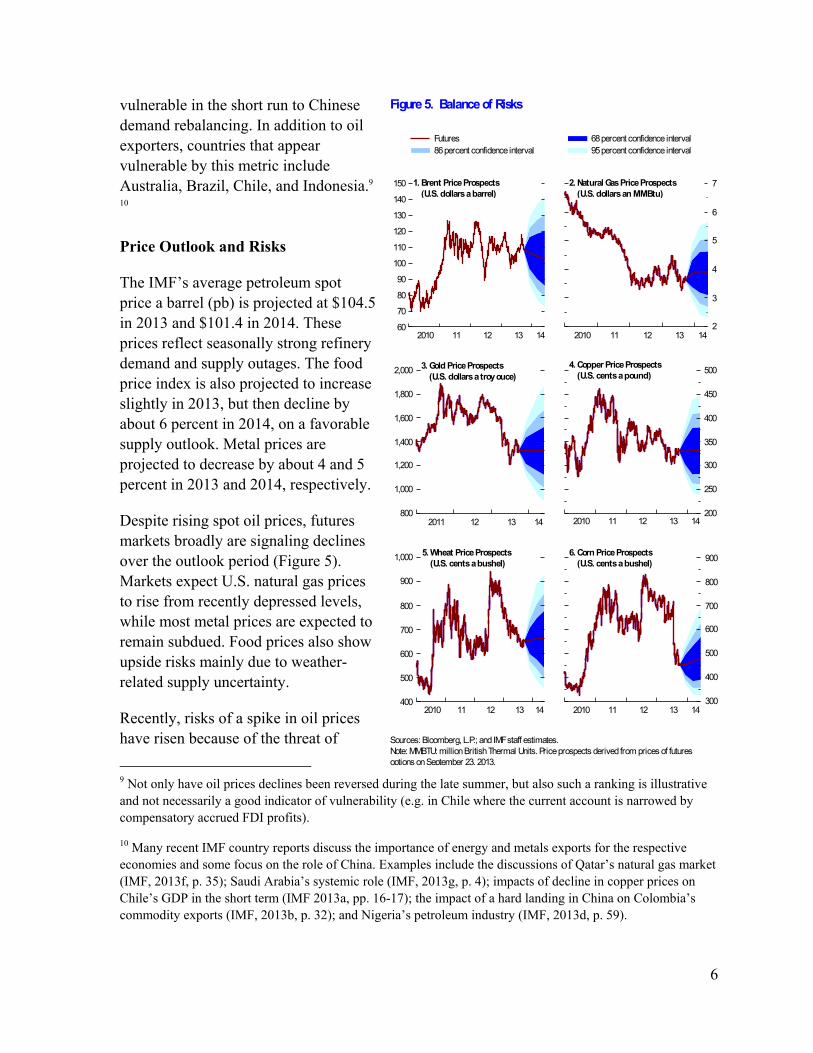
The IMF’s average petroleum spot price a barrel (pb) is projected at $104.5 in 2013 and $101.4 in 2014. These prices reflect seasonally strong refinery demand and supply outages. The food price index is also projected to increase slightly in 2013, but then decline by about 6 percent in 2014, on a favorable supply outlook. Metal prices are projected to decrease by about 4 and 5 percent in 2013 and 2014, respectively.

Despite rising spot oil prices, futures markets broadly are signaling declines over the outlook period (Figure 5). Markets expect U.S. natural gas prices to rise from recently depressed levels, while most metal prices are expected to remain subdued. Food prices also show upside risks mainly due to weather-related supply uncertainty.

Recently, risks of a spike in oil prices have risen because of the threat of

9 Not only have oil prices declines been reversed during the late summer, but also such a ranking is illustrative and not necessarily a good indicator of vulnerability (e.g. in Chile where the current account is narrowed by compensatory accrued FDI profits).

10 Many recent IMF country reports discuss the importance of energy and metals exports for the respective economies and some focus on the role of China. Examples include the discussions of Qatar’s natural gas market (IMF, 2013f, p. 35); Saudi Arabia’s systemic role (IMF, 2013g, p. 4); impacts of decline in copper prices on Chile’s GDP in the short term (IMF 2013a, pp. 16-17); the impact of a hard landing in China on Colombia’s commodity exports (IMF, 2013b, p. 32); and Nigeria’s petroleum industry (IMF, 2013d, p. 59).

200

250

300

350

400

450

500

2010 11 12 13 14

2

3

4

5

6

7

2010 11 12 13 14

Figure 5. Balance of Risks

1. Brent Price Prospects (U.S. dollars a barrel)

Sources: Bloomberg, L.P.; and IMF staff estimates.Note: MMBTU: million British Thermal Units. Price prospects derived from prices of futures options on September 23, 2013.

Futures 68 percent confidence interval86 percent confidence interval 95 percent confidence interval

4. Copper Price Prospects (U.S. cents a pound)

3. Gold Price Prospects (U.S. dollars a troy ouce)

2. Natural Gas Price Prospects (U.S. dollars an MMBtu)

60

70

80

90

100

110

120

130

140

150

2010 11 12 13 14

5. Wheat Price Prospects (U.S. cents a bushel)

6. Corn Price Prospects (U.S. cents a bushel)

800

1,000

1,200

1,400

1,600

1,800

2,000

2011 12 13 14

400

500

600

700

800

900

1,000

2010 11 12 13 14300

400

500

600

700

800

900

2010 11 12 13 14

7

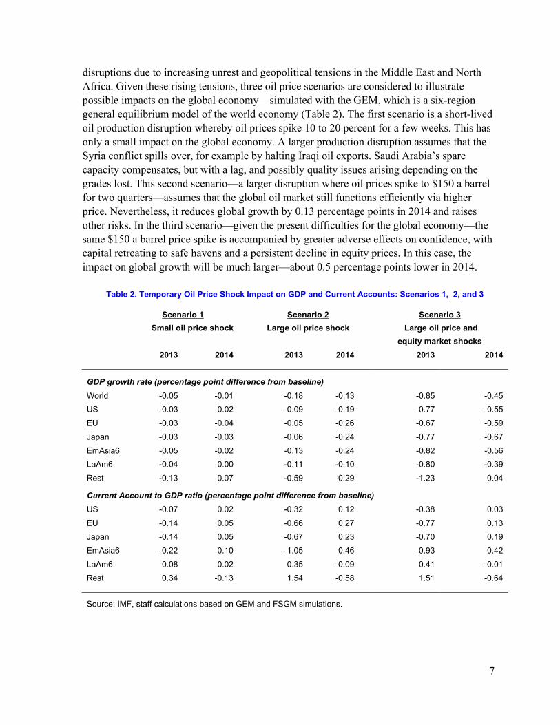
disruptions due to increasing unrest and geopolitical tensions in the Middle East and North Africa. Given these rising tensions, three oil price scenarios are considered to illustrate possible impacts on the global economy—simulated with the GEM, which is a six-region general equilibrium model of the world economy (Table 2). The first scenario is a short-lived oil production disruption whereby oil prices spike 10 to 20 percent for a few weeks. This has only a small impact on the global economy. A larger production disruption assumes that the Syria conflict spills over, for example by halting Iraqi oil exports. Saudi Arabia’s spare capacity compensates, but with a lag, and possibly quality issues arising depending on the grades lost. This second scenario—a larger disruption where oil prices spike to $150 a barrel for two quarters—assumes that the global oil market still functions efficiently via higher price. Nevertheless, it reduces global growth by 0.13 percentage points in 2014 and raises other risks. In the third scenario—given the present difficulties for the global economy—the same $150 a barrel price spike is accompanied by greater adverse effects on confidence, with capital retreating to safe havens and a persistent decline in equity prices. In this case, the impact on global growth will be much larger—about 0.5 percentage points lower in 2014.

Table 2. Temporary Oil Price Shock Impact on GDP and Current Accounts: Scenarios 1, 2, and 3

Scenario 1 Scenario 2 Scenario 3

Small oil price shock Large oil price shock Large oil price and

equity market shocks

2013 2014 2013 2014 2013 2014

GDP growth rate (percentage point difference from baseline)

World -0.05 -0.01 -0.18 -0.13 -0.85 -0.45

US -0.03 -0.02 -0.09 -0.19 -0.77 -0.55

EU -0.03 -0.04 -0.05 -0.26 -0.67 -0.59

Japan -0.03 -0.03 -0.06 -0.24 -0.77 -0.67

EmAsia6 -0.05 -0.02 -0.13 -0.24 -0.82 -0.56

LaAm6 -0.04 0.00 -0.11 -0.10 -0.80 -0.39

Rest -0.13 0.07 -0.59 0.29 -1.23 0.04

Current Account to GDP ratio (percentage point difference from baseline)

US -0.07 0.02 -0.32 0.12 -0.38 0.03

EU -0.14 0.05 -0.66 0.27 -0.77 0.13

Japan -0.14 0.05 -0.67 0.23 -0.70 0.19

EmAsia6 -0.22 0.10 -1.05 0.46 -0.93 0.42

LaAm6 0.08 -0.02 0.35 -0.09 0.41 -0.01

Rest 0.34 -0.13 1.54 -0.58 1.51 -0.64

Source: IMF, staff calculations based on GEM and FSGM simulations.

8

Economic Impacts of the U.S. Energy Boom

The United States is experiencing a boom in energy production. Natural gas output increased 25 percent, and crude oil and other liquids increased 30 percent during the past five years, reducing net oil imports by nearly 40 percent. The U.S. Energy Information Administration (EIA, 2013) baseline scenario shows U.S. production of tight oil increasing until 2020 before falling off during the next two decades.11 The baseline also shows U.S. shale gas production increasing steadily until 2040 (Figure 6). The United States is expected to be a net exporter of natural gas in the 2020s.

Simulations from a large-scale model (GEM) suggest modest impacts of the energy boom on U.S. output.12 In GEM, energy is produced by combining capital and labor with a fixed factor, which can be thought of as known reserves. As discussed above, EIA expects production of tight oil and shale gas to increase in coming years but there is uncertainty about the duration and extent of the increase. The model is simulated under the assumption that there is an increase in energy production over the next 12 years so that by the end of this time horizon production has increased by 1.8 percent of GDP.13 Figure 1.SF.7 shows the results from the model simulations.

11 Tight oil is petroleum found in formations of low permeability, generally shale or tight sandstone.

12 This discussion is taken from “Potential Implications of the United States Becoming Energy Self Sufficient,” by Ben Hunt and Dirk Muir, draft, August 2013.

13 This scenario is implemented in GEM by gradually increasing the fixed factor in oil production over the 12-year period by enough so that, once capital and labor have responded endogenously, U.S. energy production has increased by 1.8 percent of GDP. IMF (2013j) presents the results from a scenario in which the increase in energy production is 0.45 percent of GDP; the results are similar to those presented here, except that the magnitude of the effect on GDP is roughly a fourth of that shown here.

5

6

7

8

9

10

11

2012 13 14 15 20 25 30 35 40

1.0

1.5

2.0

2.5

3.0

3.5

4.0

4.5

5.0

5.5

2012 13 14 15 20 25 30 35 40

Sources: U.S. Energy Information Administration (EIA); and IMF staff calculations.

Figure 6. U.S. Oil and Gas Production Projections

EIA baseline scenario EIA low resource scenario

EIA high resource scenario

1. Tight Oil Production Projections (million barrels a day)

2. Shale Gas Production Projections (trillion cubic feet)

9

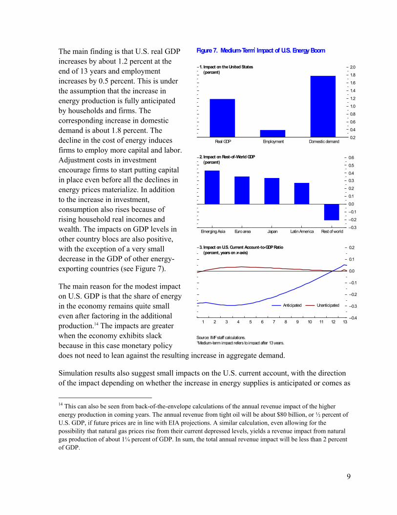
The main finding is that U.S. real GDP increases by about 1.2 percent at the end of 13 years and employment increases by 0.5 percent. This is under the assumption that the increase in energy production is fully anticipated by households and firms. The corresponding increase in domestic demand is about 1.8 percent. The decline in the cost of energy induces firms to employ more capital and labor. Adjustment costs in investment encourage firms to start putting capital in place even before all the declines in energy prices materialize. In addition to the increase in investment, consumption also rises because of rising household real incomes and wealth. The impacts on GDP levels in other country blocs are also positive, with the exception of a very small decrease in the GDP of other energy-exporting countries (see Figure 7).

The main reason for the modest impact on U.S. GDP is that the share of energy in the economy remains quite small even after factoring in the additional production.14 The impacts are greater when the economy exhibits slack because in this case monetary policy does not need to lean against the resulting increase in aggregate demand.

Simulation results also suggest small impacts on the U.S. current account, with the direction of the impact depending on whether the increase in energy supplies is anticipated or comes as

14 This can also be seen from back-of-the-envelope calculations of the annual revenue impact of the higher energy production in coming years. The annual revenue from tight oil will be about $80 billion, or ½ percent of U.S. GDP, if future prices are in line with EIA projections. A similar calculation, even allowing for the possibility that natural gas prices rise from their current depressed levels, yields a revenue impact from natural gas production of about 1¼ percent of GDP. In sum, the total annual revenue impact will be less than 2 percent of GDP.

0.2

0.4

0.6

0.8

1.0

1.2

1.4

1.6

1.8

2.0

Real GDP Employment Domestic demand

Source: IMF staff calculations. 1Medium-term impact refers to impact after 13 years.

Figure 7. Medium-Term1 Impact of U.S. Energy Boom

–0.3

–0.2

–0.1

0.0

0.1

0.2

0.3

0.4

0.5

0.6

Emerging Asia Euro area Japan Latin America Rest of world

1. Impact on the United States (percent)

2. Impact on Rest-of-World GDP (percent)

–0.4

–0.3

–0.2

–0.1

0.0

0.1

0.2

1 2 3 4 5 6 7 8 9 10 11 12 13

3. Impact on U.S. Current Account-to-GDP Ratio (percent, years on x-axis)

Anticipated Unanticipated

10

a surprise. In both cases, the improvement in the energy component of the trade balance is offset by a decline in the non-energy balance. In the case where the increase in energy supplies is fully anticipated, U.S. households and corporations temporarily increase borrowing from abroad to support higher consumption (anticipating the wealth increase from higher energy production) and investment. The appreciation of the U.S. dollar reduces import prices and also contributes to the increase in the non-energy balance. Overall, the result is a small decline in the current account balance.

In the case where the increase in energy production comes as a surprise each year, consumption and investment respond more gradually as households do not anticipate the magnitude of the increase in their wealth and firms do not anticipate the extent of the decline in the cost of production. With domestic demand responding more gradually, the increase in non-energy imports is also smaller and it is offset by the increase in the energy balance. Econometric evidence on the impact of giant discoveries of oil and gas on the current account is presented in Box 1.

Though its aggregate effects on output are likely to be small, the energy boom has disrupted historical relationships between energy prices. Brent and West Texas Intermediate, two major pricing benchmarks for crude oil, have moved together for three decades, but have diverged in recent years (Box 2). Oil and natural gas prices have also moved in tandem within and across countries as a result of substitution and international arbitrage. Since 2009, however, U.S. natural gas prices have decoupled from U.S. oil prices while prices elsewhere continue to move together, as shown for Germany (Figure 8). Restoration of the law of one price could take several years, particularly given regulatory and technological barriers to U.S. exports, and the link to oil prices in Asia and Europe.15

15 As discussed in Loungani and Matsumoto (forthcoming), over time more consumers will be able to make the initial investment needed to switch their energy sources from crude oil (or coal) to natural gas. Natural gas price

(continued)

0

50

100

150

200

250

300

2006 07 08 09 10 11 12 May 13

Sources: U.S. Bureau of Labor Statistics; Statistisches Bundesamt; and IMF staff calculations.

Figure 8. Natural Gas and Oil Prices in the United Statesand Germany(2005 = 100)

Natural gas Oil

80

100

120

140

160

180

200

220

240

260

2006 07 08 09 10 11 12 May 13

1. United States

2. Germany

11

Box 1. Energy Booms and the Current Account: Cross-Country Experience16

Discoveries of giant oil and gas fields—fields containing ultimate recoverable reserves equivalent to at least 500 million barrels—have been relatively widespread across countries since the 1970s. These discoveries constitute a unique source of exogenous future income shocks. Regression results, using a panel of 178 countries over the period 1970 to 2012, show that the effect of these discoveries was first to decrease the current account balance and then to increase it before the effect leveled off (Figure 1.1).17 Hence, the pattern of the effect is similar to the case of the unanticipated increase in energy production shown in the IMF Global Economic Model (GEM) simulations. The regression estimates imply that a discovery equal to the size of proven reserves in U.S. unconventional energy in the United States would lead at its peak to about a 0.1 percent of GDP increase in the U.S. current account balance.

The effect thus is small, as also suggested by the GEM simulations. There are cases where oil and gas discoveries have had larger effects on the current account, but the size of those discoveries was larger than the expected increase in the case of the United States. For instance, the share of North Sea oil discoveries in U.K. GDP was about 6 to 7 percent at its peak. After initially moving in line with the sharp increase and decline in oil revenues, the U.K. current account decoupled from oil revenues, which have remained low and stable at about 1½ percent of GDP since 1990. The impact on the current account was larger in Norway because of the much larger share of the gas and oil

differentials across countries will also diminish if other countries start to extract their own shale gas reserves or if environmental concerns slow extraction in the United States. In June 2013, the EIA released estimates suggesting that shale oil resources worldwide would add roughly 10 percent to global oil reserves, while shale gas resources would nearly double the world’s supply of natural gas resources.

16 The author of this box is Rabah Arezki.

17 Details are given in Arezki and Sheng (forthcoming).  

Figure 1.1. Giant Oil and GasDiscoveries and the Current Account

Source: IMF staff calculations.

10

20

30

40

50

60

70

80

90

1970s 1980s 1990s 2000s 2010–12

1. Discoveries (oil and gas field discoveries, by year)

2. Oil Discoveries and Current Account (years after discovery, regression coefficient)

–0.06

–0.04

–0.02

0.00

0.02

0.04

0.06

0.08

–2 0 2 4 6 8 10 12 14 16 18 20

Coefficient Confidence interval

12

extraction sector in the economy—nearly 25 percent—and the country’s fiscal policy of keeping most of the oil revenues in a special fund.

Box 2. Oil Price Drivers and the Narrowing WTI-Brent Spread18

In recent years, West Texas Intermediate (WTI) prices fell substantially below Brent prices as a supply surge from unconventional energy sources in the United States and Canada, and difficulties in moving this supply to U.S. refining hubs led to a build-up of inventories. But the differential has narrowed this year (Figure 2.1).

To understand fundamental oil price drivers, a sign-restricted structural vector autoregressive model is estimated using four variables: global crude oil production, global industrial production, the real price of Brent crude oil, and Organization for Economic Cooperation and Development crude oil inventories (to proxy speculative demand) for the period 1983:Q1-2013:Q3 (see Beidas-Strom and Pescatori, 2013). Speculation motives include both decisions of adjusting oil inventories in anticipation of future price movements and behavior induced by possible mispricing in financial (oil derivatives) markets. Figures 2.2 and 2.3 show that Brent prices are largely driven by flow demand and speculative demand shocks (blue and green bars, respectively).19 Brent competes more closely with North and West African and Middle Eastern crude oil varieties, hence its price is more exposed to precautionary demand stemming from geopolitical risk. Risk premiums and the prevailing Brent futures term structure also attract financial investors.

18 The author of this box is Samya Beidas-Strom.

19 If the sum of the bars is increasing over time, shocks exert upward pressure on the oil price, and vice versa.

Figure 2.1. WTI–Brent Price Differentials(U.S. dollars a barrel)

–30

–25

–20

–15

–10

–5

0

5

10

2007 08 09 10 11 12 13

Sources: Bloomberg, L.P.; and IMF staff calculations.

Price differential Ten-year average spread

Figure 2.2. Brent SVAR HistoricalDecomposition(Left axis: contribution of shocks, percent; right-axis: U.S.dollars a barrel)

–1.0

–0.8

–0.6

–0.4

–0.2

0.0

0.2

0.4

0.6

0.8

1.0

10

30

50

70

90

110

130

2000 02 04 06 08 10 12 13

Source: IMF staff calculations. Note: SVAR = structural vector autogression.

Real oil price (right scale)

Flow oil supply shock Flow demand shock

Residual shock Speculative shock

13

Replacing Brent with WTI prices, the model suggests that before 2007 the drivers of the two leading benchmark prices are almost identical. However, since 2007, WTI prices have been influenced more by global supply conditions (burgundy bars)—particularly the boom in North American supply and crude oil transportation constraints since 2009—and less by speculative demand. More recently, infrastructure bottlenecks have eased (yellow bars) and speculative and seasonal demand increased, raising WTI and narrowing the spread. But this narrowing may not prove durable. Seasonal U.S. demand will dissipate in the third quarter, and sufficient crude oil infrastructure to carry oil from the middle of the United States to the Gulf coast will not be reconfigured and completed until late next year. Therefore, downward pressures on WTI could continue, altering the WTI futures term structure and lowering recent investor interest.

Figure 2.3. WTI–Brent Differential Historical Decomposition(Contribution of shocks, percent)

–0.6

–0.4

–0.2

0.0

0.2

0.4

0.6

2000 02 04 06 08 10 12

Source: IMF staff calculations.

Flow oil supply shock Flow demand shockResidual shock Speculative shock