combining static analysis and testing for …mizuhito/thesis/dothibichngoc.pdfroundoff error...
TRANSCRIPT
Combining Static Analysis and Testing
for Overflow and Roundoff Error Detection
by
DO THI BICH NGOC
submitted toJapan Advanced Institute of Science and Technology
in partial fulfillment of the requirementsfor the degree of
Doctor of Philosophy
Supervisor: Professor Mizuhito Ogawa
School of Information ScienceJapan Advanced Institute of Science and Technology
July 13, 2010
Abstract
In computer algorithms, real numbers are often represented as floating point numbers.
However, hardware typically uses fixed point number representations for lower cost and
higher speed. Direct transformations from a reference algorithm to a hardware algorithm
with fixed point numbers often cause different computational results because of overflow
errors and roundoff errors. Hence, when implementing hardware algorithms we need to
consider: (1) whether overflow errors occur or not and (2) whether the roundoff errors
exceed a predefined threshold bound or not.
The problem of detecting overflow and roundoff errors has been studied since 1960s,
and is still an active research area. Originally, overflow and roundoff errors are often
detected manually by using mathematical reasoning or testing. Recently, there are some
extensive works of automatically checking overflow and roundoff errors based on static
analysis and abstraction. In order to abstract overflow and roundoff errors, there are
two well known techniques. The first technique is Classical interval (CI) which keeps the
possible lowest and highest values as a segment. The second technique is Affine interval
(AI) which introduces symbolic manipulations on noise symbols, to handle correlations
between variables. AI arithmetic supplies higher precision than CI one. However, for
nonlinear operations, AI arithmetic requires to introduce a fresh noise symbol each time.
A question naturally raised is that: can we construct new interval arithmetic such that it
is simpler than AI but as precise as AI?
It is worth emphasizing that static analysis is useful in automatically proving safety
properties of programs but it may return spurious counterexamples due to approximation.
In contrast, testing can return exact roundoff errors, while it virtually cannot cover all
possible inputs. The challenge is: how to bridge the gap between testing and static
analysis?
Motivated by the above questions, this thesis is concerned about the problem of de-
tecting overflow and roundoff errors when converting floating point numbers to fixed point
numbers for a class of C programs with bounded loops, fixed size arrays, and no pointer
manipulations. This class of programs is sufficient to capture the core algorithms of DSP
encoders/decoders. The contributions and achievements of this thesis are summarized as
follows:
• New intervals: improve current intervals (i.e., CI and AI) to approximate overflow
and roundoff errors. Two new intervals named “Extended affine interval” (EAI) and
“Positive-noise affine interval” (PAI) are proposed. EAI represent ranges as AI form
i
whose each noise symbol is assigned a CI. By this means, the results of nonlinear
operations can be approximated to keep linear form without introducing new noise
symbols as AI does. In positive-noise AI, the noise symbols in PAI lie in [0,1]
(instead of [-1,1]) and the nonlinear operations are designed based on Chebyshev
approximation to improve the precisions.
• Overflow and roundoff error analysis as weighted model checking: propose and im-
plement the overflow and roundoff error analysis based on weighted model checking.
The overflow and roundoff error abstractions based on intervals (CI, AI, and EAI)
are used to create sets of weights. Then, a C program is modeled by a weighted
transition system (a finite transition system + weight domain), where weight do-
main is generated by an on-the-fly manner. Finally, the overflow and roundoff error
problem was reduced to checking reachability properties for the weighted transition
system. The proposed framework is implemented in an automatic overflow and
roundoff error analyzer, called CANA (C ANAlyzer). Experimental results on small
programs show that the EAI is much more precise than CI.
• Combine static analysis and testing for roundoff error detection: propose and imple-
ment a hybrid approach called “counterexample-guided narrowing” in which analysis
and testing refine each other. This approach is applied to improve the precision of
roundoff error analysis and implement the proposed framework as a prototype tool
CANAT (C ANAlyzer and Tester). Although our experiments are still small, the
results outperforms both random test and static analysis.
Key words: software verification, static analysis, model checking, testing, roundoff
error, overflow error, affine interval.
ii
Acknowledgments
This thesis would not have been possible without the help of many people. First of all,
I would like to express my deep gratitude to my principal supervisor, Professor Mizuhito
Ogawa. He has been a good and patient advisor. I learned much from him how to be a
researcher. It would be impossible to pinpoint his contributions large and small to this
work; his encouragement has been very important as well. Without him, this thesis would
simply not exist.
That the thesis does not exist in the present form is due also to the enthusiastic interest,
support, and criticism I have received from my colleagues and members of my reading
thesis committees, Professor. Kokichi Futatsugi, Professor. Shin Nakajima, Professor.
Kazuhiro Ogata, Professor. Toshiaki Aoki, and Dr. Hirokazu Anai. I have greatly
benefited from their guidance and helpful comments. This thesis was markedly improved
because of their critical reading and valuable suggestions. Especially, I would also like
to give special thanks to Professor Toshiaki Aoki for his supervision of my sub-theme
research.
The faculty, staff and students at the Software Verification Laboratory have provided
an excellent academic environment; in particular, Associate Professor Fumihiko Asano,
Assistant Professor Nao Hirokawa, Dr. Li Xin, Dr Li Gouqiang, Dr Nguyen Van Tang, Mr
Klein Dominik, Mr Song Lin, Mr To Van Khanh. Our technical discussions have helped
in my work, while our more philosophical discussions have been thoroughly enjoyable.
Especially, I would like to thank Nao for his valuable guidance and technical supports to
this thesis.
My Vietnamese friends have made my stay in JAIST fun, exciting and memorable.
I would like to thank my best friends Nguyen Quang Huy, Pham Gia Vinh Anh who
always encourage and support me in research whenever I need. I thank the teachers in
the Technical Communication Program Office - who helped me to refine my technical
drafts of papers and thesis.
Finally, I would also like to take this opportunity to thank my family for their love and
supports; especially, for my parents for encouraging me, and for my husband for being
my best friend and supporting me. I dedicate this thesis to my son Nguyen Nhat Hung,
who provided me with many joyous moments. Whenever I needed to clean my head from
all this verification stuff he was ready to give me plenty of other things to do. Without
the joy of having him I am not sure I would have completed this task.
iii
Contents
Abstract i
Acknowledgments iii
1 Introduction 2
1.1 Sources of Numerical Errors . . . . . . . . . . . . . . . . . . . . . . . . . . 2
1.2 Overflow and Roundoff Errors Problem . . . . . . . . . . . . . . . . . . . . 3
1.3 The Existing Approaches . . . . . . . . . . . . . . . . . . . . . . . . . . . . 7
1.4 The Proposed Approach and Contributions of the Thesis . . . . . . . . . . 9
1.5 Structure of the Thesis . . . . . . . . . . . . . . . . . . . . . . . . . . . . . 10
2 Representation of Real Numbers in Computer and the ORE Problem 12
2.1 Floating Point Numbers and ORE problem . . . . . . . . . . . . . . . . . . 12
2.1.1 Floating Point Numbers . . . . . . . . . . . . . . . . . . . . . . . . 12
2.1.2 OREs of Floating point Numbers . . . . . . . . . . . . . . . . . . . 13
2.2 Fixed Point Numbers and ORE Problem . . . . . . . . . . . . . . . . . . . 15
2.2.1 Fixed Point Numbers . . . . . . . . . . . . . . . . . . . . . . . . . . 15
2.2.2 OREs of Fixed point Numbers . . . . . . . . . . . . . . . . . . . . . 16
2.3 ORE Arithmetic . . . . . . . . . . . . . . . . . . . . . . . . . . . . . . . . 17
2.3.1 Real-to-Fixed ORE Arithmetic . . . . . . . . . . . . . . . . . . . . 17
2.3.2 Real-to-Float ORE Arithmetic . . . . . . . . . . . . . . . . . . . . . 19
2.3.3 Float-to-Fixed ORE Arithmetic . . . . . . . . . . . . . . . . . . . . 20
2.4 ORE Constraints of the Programs . . . . . . . . . . . . . . . . . . . . . . . 22
3 Dataflow Analysis as Weighted Model Checking 26
3.1 Dataflow Analysis as Model Checking and Abstraction . . . . . . . . . . . 27
3.1.1 Dataflow Analysis . . . . . . . . . . . . . . . . . . . . . . . . . . . . 27
3.1.2 Model Checking . . . . . . . . . . . . . . . . . . . . . . . . . . . . . 28
3.1.3 Dataflow Analysis as Model Checking and Abstraction . . . . . . . 30
3.2 Dataflow Analysis as Weighted Model Checking Problem . . . . . . . . . . 33
3.2.1 Weighted Model Checking . . . . . . . . . . . . . . . . . . . . . . . 33
3.2.2 Dataflow Analysis as Weighted Model Checking and Abstraction . . 35
iv
3.2.3 On-the-fly Weight Creation for an Acyclic Model . . . . . . . . . . 36
4 Interval Arithmetics in ORE Propagation 37
4.1 Classical Interval . . . . . . . . . . . . . . . . . . . . . . . . . . . . . . . . 37
4.2 Affine Interval . . . . . . . . . . . . . . . . . . . . . . . . . . . . . . . . . . 39
4.3 Extended Affine Interval . . . . . . . . . . . . . . . . . . . . . . . . . . . . 43
4.4 Positive-noise Affine Interval . . . . . . . . . . . . . . . . . . . . . . . . . . 46
4.5 Interval Representations by Floating point Numbers . . . . . . . . . . . . . 49
5 Abstraction for ORE Problem 52
5.1 CI Abstraction for ORE Problem . . . . . . . . . . . . . . . . . . . . . . . 52
5.2 AI Abstract Numbers . . . . . . . . . . . . . . . . . . . . . . . . . . . . . . 54
5.3 EAI Abstract Numbers . . . . . . . . . . . . . . . . . . . . . . . . . . . . . 55
5.4 Meet Operator . . . . . . . . . . . . . . . . . . . . . . . . . . . . . . . . . 57
5.5 Abstraction for ORE analysis . . . . . . . . . . . . . . . . . . . . . . . . . 58
6 ORE Analysis as Weighted Model Checking Problem 59
6.1 Weighted Domain for the ORE Problem . . . . . . . . . . . . . . . . . . . 59
6.2 Weighted Transitions for the ORE Problem . . . . . . . . . . . . . . . . . 60
6.3 ORE Analysis . . . . . . . . . . . . . . . . . . . . . . . . . . . . . . . . . . 63
6.4 Implementation and Experiments . . . . . . . . . . . . . . . . . . . . . . . 65
7 Detecting REs based on Counterexample-guided Narrowing 73
7.1 Counterexample-guided Narrowing Approach . . . . . . . . . . . . . . . . . 74
7.1.1 Observation on RE Analysis . . . . . . . . . . . . . . . . . . . . . . 74
7.1.2 Counterexample-guided Narrowing Approach . . . . . . . . . . . . . 75
7.2 Refining Test Data Generation . . . . . . . . . . . . . . . . . . . . . . . . . 76
7.2.1 Range Reduction . . . . . . . . . . . . . . . . . . . . . . . . . . . . 77
7.2.2 More Ticks for more Sensitive Noise Symbols . . . . . . . . . . . . . 78
7.3 Refinement of Analysis by Narrowing Input Domains . . . . . . . . . . . . 79
7.4 Implementation and Experiments . . . . . . . . . . . . . . . . . . . . . . . 81
8 Related Work 87
9 Conclusions 91
9.1 Summary of the Thesis . . . . . . . . . . . . . . . . . . . . . . . . . . . . 91
9.2 Future Work . . . . . . . . . . . . . . . . . . . . . . . . . . . . . . . . . . 92
References 94
Publications 100
v
List of Figures
1.1 Typical loops in Mpeg decoder . . . . . . . . . . . . . . . . . . . . . . . . . 5
1.2 An example of a C program . . . . . . . . . . . . . . . . . . . . . . . . . . 6
1.3 Results of analyzing and testing C program in Figure 1.2 . . . . . . . . . . 8
3.1 Model checker structure . . . . . . . . . . . . . . . . . . . . . . . . . . . . 29
3.2 Transition system of program in Figure 1.2 . . . . . . . . . . . . . . . . . . 31
3.3 Dataflow analysis as model checking and abstraction . . . . . . . . . . . . 32
3.4 Dataflow analysis as weighted model checking . . . . . . . . . . . . . . . . 35
4.1 Chebyshev approximation for 1:y
. . . . . . . . . . . . . . . . . . . . . . . . 41
6.1 CIL code for Example 3 . . . . . . . . . . . . . . . . . . . . . . . . . . . . 62
6.2 CFG of three address codes in Fig. 6.1 . . . . . . . . . . . . . . . . . . . . 62
6.3 ORE analysis as weighted model checking . . . . . . . . . . . . . . . . . . 64
6.4 CANA system . . . . . . . . . . . . . . . . . . . . . . . . . . . . . . . . . . 66
6.5 The analysis result of P2(x) . . . . . . . . . . . . . . . . . . . . . . . . . . 68
6.6 The analysis result of P5(x) . . . . . . . . . . . . . . . . . . . . . . . . . . 69
6.7 The analysis result of Sin(x) . . . . . . . . . . . . . . . . . . . . . . . . . . 70
6.8 The analysis result of subMpeg(exps) . . . . . . . . . . . . . . . . . . . . . 70
6.9 The analysis result of rump . . . . . . . . . . . . . . . . . . . . . . . . . . 71
6.10 The analysis result of 10-variable functions of degree ¥ 7 . . . . . . . . . . 72
7.1 Effects of decomposition of Dmax to D1max, D2
max . . . . . . . . . . . . . . 81
7.2 CANAT system . . . . . . . . . . . . . . . . . . . . . . . . . . . . . . . . . 83
vi
List of Tables
2.1 The formats of floating point numbers . . . . . . . . . . . . . . . . . . . . 13
2.2 Syntax of core language . . . . . . . . . . . . . . . . . . . . . . . . . . . . 23
2.3 Weakest precondition for ORE problem . . . . . . . . . . . . . . . . . . . . 24
6.1 Weight function of ORE analysis . . . . . . . . . . . . . . . . . . . . . . . 61
6.2 Weight function for a CIL code in Example 30 . . . . . . . . . . . . . . . . 63
7.1 Compare CANAT with CANA and random test . . . . . . . . . . . . . . . 84
7.2 Compare CANAT with Matlab test . . . . . . . . . . . . . . . . . . . . . 85
7.3 Checking result of 10-variable functions of degree ¥ 7 . . . . . . . . . . . 86
1
Chapter 1
Introduction
1.1 Sources of Numerical Errors
In general, a numerical algorithm for solving a given problem may have errors of one or
several types. Although different source initiate the error, they all cause the same effect:
diversion from the exact answer. Some errors are small and may be neglected. Others
may be devastating if overlooked. The major sources of errors are as follows.
1. Human error: is introduced during the process of solving the problem by human,
for example, changing signs in a formula or a simple programming error.
2. Truncation error: occurs when we are unable to evaluate explicitly a given quan-
tity, and replace it by an approximation that can be computed.
For example, the function sinpxq can be replaced by
sinpxq xx3
3!
x5
5! ...
We may calculate px x3
3! x5
5!q as an approximation to sinpxq, provide the error
term Epxq x7
7! ....
3. Machine error: A floating point (or fixed point) number processed by a computer
may not have an exact representation. Also, floating point (or fixed point) arith-
metic in general is not exact. For example, if the length of a mantissa is 4 bits,
then 0.1101 0.1011 0.1000 (chopping mode) whereas the exact values of the
left-hand side is 0.10001111. There are two types of machine errors : roundoff error
and overflow error.
4. Inaccurate observation: Many numerical processes involve physical quantities
such as the speed of light, density of iron, or the constants of gravity. These quanti-
ties are provided by experiments and naturally introduce some experimental errors.
2
For example, the speed of light in vacuum is
c p2.997925 εq 1010cmsec.|ε| ¤ 106
Experimental or observational errors cannot be removed or even reduced, without
improving the observational technique.
5. Modeling error: Constructing a mathematical model is the first step in the pro-
cess of solving a problem. However, an equation or a system of equations that is
expected to describe some phenomena will generally only approximate the phys-
ical reality. Occasionally a mathematical model may be solved successfully, and
yet the computed and the experimental results are far apart. This may occur if
an important physical aspect is overlooked and the mathematical model is unjustly
simplified.
Truncation errors, inaccurate observations, and modeling errors are caused by hu-
man when create numerical algorithm from real problem. Thus, they are often analyzed
manually. Human error and machine error are caused by implementing the algorithm in
computer (or hardware system). While human error can be avoided by carefully code the
algorithm, machine error cannot be avoided because of finite presentation of real num-
bers. In this thesis, we focus on automatically analyzing machine error (i.e., overflow and
roundoff errors) when converting floating point numbers to fixed point numbers.
1.2 Overflow and Roundoff Errors Problem
In the computers, the (infinite) real numbers are approximated by finite numbers (e.g.,
floating point numbers, fixed point numbers). Because of finite representation, the over-
flow and roundoff errors (OREs) may occur. There are three kinds of OREs:
1. Real numbers vs floating point numbers: approximating real numbers as floating
point numbers causes OREs. These OREs often appear in computers since most of
them use floating point arithmetic. Most of ORE researches focus on this kind of
OREs [13, 26].
2. Real numbers vs fixed point numbers: OREs may occur when real numbers are
approximated as fixed point numbers. This kind of errors appears when implement
a (reference) algorithm with real numbers in a hardware with fixed point numbers
[32].
3. Floating point numbers vs fixed point numbers: many algorithms implemented
in computers are proved to be satisfied the ORE requirement. We also want to
re-implement them in hardware systems or devices, such as, PDA, mp3 players,
videogame consoles. These devices need to convert the floating point numbers to
3
fixed point numbers for lower cost and higher speed. Recently, there are many works
focus on converting floating point numbers to fixed point numbers [3, 5, 44, 58, 59].
Because the floating point numbers can represent more precise values than that of
fixed point numbers, the conversation from floating point numbers to fixed point
numbers may causes OREs.
The OREs will be propagated through computations of the program. Further, the
computations themselves also cause OREs because the arithmetic needs to round the
result to fit the number format. Besides, OREs are also affected by types of statements
(e.g., branch, loop, assignment). OREs sometimes are propagated too much and may
cause serious problems. One example about disaster causes by roundoff error is “The
Patriot Missile Failure” 1.
Example 1 On February 25, 1991, during the Gulf War, an American Patriot Missile
battery in Dharan, Saudi Arabia, failed to track and intercept an incoming Iraqi Scud
missile. The Scud struck an American Army barracks, killing 28 soldiers and injuring
around 100 other people.
The reason is roundoff error when representing real number 110 by fixed point num-
ber. The number 110 equals 12412512812912121213.... In other words,
the binary expansion of 110 is 0.0001100110011001100110011001100.... Now the 24 bit
register in the Patriot stored instead 0.00011001100110011001100 introducing an error of
0.0000000000000000000000011001100... binary, or about 0.000000095 decimal. Multiply-
ing by the number of tenths of a second in 100 hours gives 0.0000000951006060 10
0.34. A Scud travels at about 1,676 meters per second, and thus travels more than half of
kilometer in this time.
Another example about disaster cause by overflow error is “The Explosion of the
Ariane 5” 2.
Example 2 On 1996 June 4, an unmanned Ariane 5 rocket launched by the European
Space Agency exploded just forty seconds after its lift-off from Kourou, French Guiana.
The destroyed rocket and its cargo were valued at $500 million.
The cause of the failure was a software error in the inertial reference system. Specif-
ically a 64 bit floating point number relating to the horizontal velocity of the rocket with
respect to the platform was converted to a 16 bit signed integer. The number was larger
than 32767, the largest integer storable in a 16 bit signed integer, and thus the conversion
failed.
Target programs
1http://www.ima.umn.edu/ arnold/disasters/patriot.html2http://www.ima.umn.edu/ arnold/disasters/ariane.html
4
Motivated by practical demands, our target programs are reference C algorithms for
DSP encoders and DSP decoders.
Our observation on DSP encoders/decoders is that they contain unbounded loops,
pointers manipulation, dynamic arrays manipulation only in the outermost interface of
large input data (e.g., sound, video). The input data are divided into small pieces and
processed by the core algorithm (e.g., Invert Direct Cosine Transform algorithm), which
(mainly) consists of loops with a bounded number of iterations and arrays with a fixed
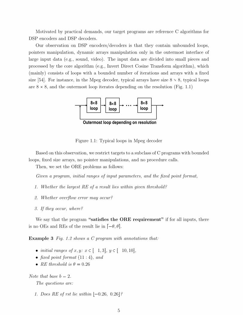
size [54]. For instance, in the Mpeg decoder, typical arrays have size 8 8, typical loops
are 8 8, and the outermost loop iterates depending on the resolution (Fig. 1.1)
8×8loop
…
Outermost loop depending on resolution
8×8loop
8×8loop
Figure 1.1: Typical loops in Mpeg decoder
Based on this observation, we restrict targets to a subclass of C programs with bounded
loops, fixed size arrays, no pointer manipulations, and no procedure calls.
Then, we set the ORE problems as follows:
Given a program, initial ranges of input parameters, and the fixed point format,
1. Whether the largest RE of a result lies within given threshold?
2. Whether overflow error may occur?
3. If they occur, where?
We say that the program “satisfies the ORE requirement” if for all inputs, there
is no OEs and REs of the result lie in rθ, θs.
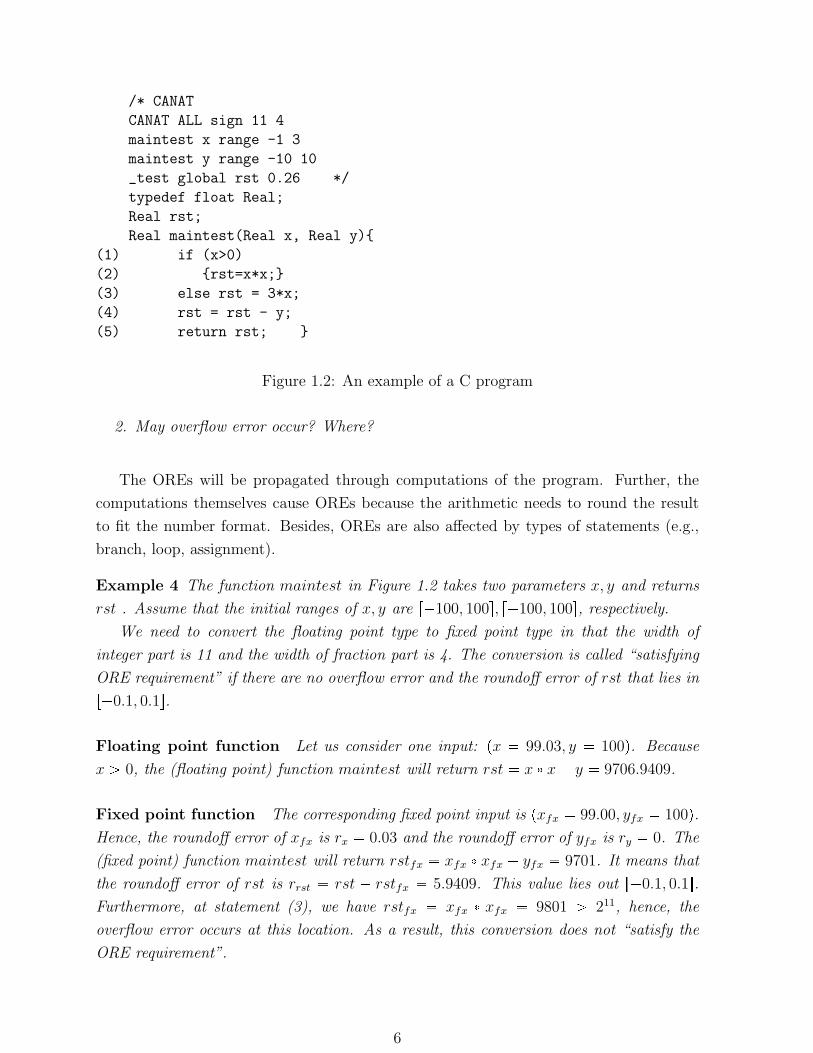
Example 3 Fig. 1.2 shows a C program with annotations that:
• initial ranges of x, y: x P r1, 3s, y P r10, 10s,
• fixed point format p11 : 4q, and
• RE threshold is θ 0.26
Note that base b 2.
The questions are:
1. Does RE of rst lie within r0.26, 0.26s?
5
/* CANAT
CANAT ALL sign 11 4
maintest x range -1 3
maintest y range -10 10
_test global rst 0.26 */
typedef float Real;
Real rst;
Real maintest(Real x, Real y)
(1) if (x>0)
(2) rst=x*x;
(3) else rst = 3*x;
(4) rst = rst - y;
(5) return rst;
Figure 1.2: An example of a C program
2. May overflow error occur? Where?
The OREs will be propagated through computations of the program. Further, the
computations themselves cause OREs because the arithmetic needs to round the result
to fit the number format. Besides, OREs are also affected by types of statements (e.g.,
branch, loop, assignment).
Example 4 The function maintest in Figure 1.2 takes two parameters x, y and returns
rst . Assume that the initial ranges of x, y are r100, 100s, r100, 100s, respectively.
We need to convert the floating point type to fixed point type in that the width of
integer part is 11 and the width of fraction part is 4. The conversion is called “satisfying
ORE requirement” if there are no overflow error and the roundoff error of rst that lies in
r0.1, 0.1s.
Floating point function Let us consider one input: px 99.03, y 100q. Because
x ¡ 0, the (floating point) function maintest will return rst x x y 9706.9409.
Fixed point function The corresponding fixed point input is pxfx 99.00, yfx 100q.
Hence, the roundoff error of xfx is rx 0.03 and the roundoff error of yfx is ry 0. The
(fixed point) function maintest will return rstfx xfx xfx yfx 9701. It means that
the roundoff error of rst is rrst rst rstfx 5.9409. This value lies out r0.1, 0.1s.
Furthermore, at statement (3), we have rstfx xfx xfx 9801 ¡ 211, hence, the
overflow error occurs at this location. As a result, this conversion does not “satisfy the
ORE requirement”.
6
1.3 The Existing Approaches
OREs are sources of serious bugs that affect economy, or even cause deaths. Therefore,
ORE detection has been attracted many attention over the past fifty years (since 1960s)
[21, 26, 13, 14, 45, 51]. There are main existing approaches for these problems such as
mathematical reasoning, numerical analysis, and testing. In the following, we are going
to give a survey on these main approaches.
Mathematical reasoning
In the mathematical reasoning [21], the user approximates an ORE formula by inequations
and mathematical transformations. Mathematical reasoning method normally returns
precise results but user may take monthly to solve the ORE formula.
Testing OREs
The OREs when approximating real numbers to floating point (or fixed point) numbers
cannot be tested automatically. The reason is the computer cannot represent (infinite)
real numbers. However, the OREs between program with floating point arithmetic (Pflt)
and the corresponding program with fixed point (Pfxp) can be computed [63]. An overflow
error will occur when the result of a fixed point operation in Pfxp exceeds the range that
fixed point number can represent. A (true) roundoff error is the difference between the
execution of Pflt and Pfxp. The ORE testing problem is: whether there is an input such
that OREs occur or its roundoff error does not lie in a given roundoff error threshold
bound rθ, θs? If there exists such an input, we call it a counterexample.
Test data depends on both the input domain and the strategy of generating test data.
For example, assuming that a program has 5 variables, each variable is initiated with
range r0, 255s. For each variable, we choose 4 instances for both the fixed point part and
roundoff error part. Then, the number of test cases is 452 (about one million). This is a
huge number, and testing becomes infeasible. The challenge of testing method is how to
generate a set of test data that can cover all cases of the program with a small number
of tests.
Static analysis OREs
From the viewpoint of abstract interpretation [9, 57], a static analysis determines ORE
properties of a program by exhausting executions under abstraction, which propagates
the ranges of both fixed point parts and roundoff errors from the begin to the end of
the program [26, 51]. There are two main techniques to represent ranges. The first
method uses classical interval (CI) [2, 47], which keeps the possible lowest and highest
values as a segment. This method is simple but imprecise, because it does not handle
7
the correlations among variables. The second method uses affine interval (AI) [61, 62],
which introduces symbolic manipulations on noise symbols, to handle correlations between
variables. AI arithmetic supplies higher precision than CI one. However, for nonlinear
operations (e.g., multiplication), AI arithmetic requires to introduce a fresh noise symbol
each time. This leads to high complexity if there are many nonlinear operations. In order
to improve efficiency and precision of the analysis, a question naturally raised is that: can
we construct a new interval arithmetic such that it is better than CI and AI? Further,
the over approximations occur at the control flows (such as the conditional branches and
loops) and operations of the programs. Another question is how to reduce this over
approximation.
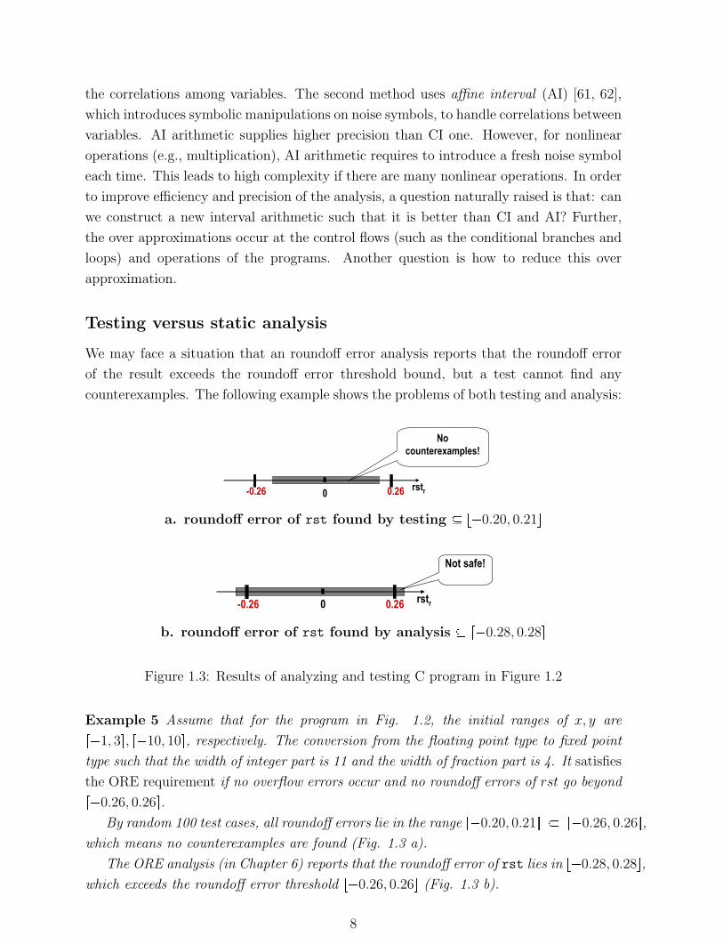
Testing versus static analysis
We may face a situation that an roundoff error analysis reports that the roundoff error
of the result exceeds the roundoff error threshold bound, but a test cannot find any
counterexamples. The following example shows the problems of both testing and analysis:-0.26 0.260 rstr
-0.26 0.260 rstr
Not safe!
No counterexamples!
a. roundoff error of rst found by testing r0.20, 0.21s
-0.26 0.260 rstr
-0.26 0.260 rstr
Not safe!
No counterexamples!
b. roundoff error of rst found by analysis r0.28, 0.28s
Figure 1.3: Results of analyzing and testing C program in Figure 1.2
Example 5 Assume that for the program in Fig. 1.2, the initial ranges of x, y are
r1, 3s, r10, 10s, respectively. The conversion from the floating point type to fixed point
type such that the width of integer part is 11 and the width of fraction part is 4. It satisfies
the ORE requirement if no overflow errors occur and no roundoff errors of rst go beyond
r0.26, 0.26s.
By random 100 test cases, all roundoff errors lie in the range r0.20, 0.21s r0.26, 0.26s,
which means no counterexamples are found (Fig. 1.3 a).
The ORE analysis (in Chapter 6) reports that the roundoff error of rst lies in r0.28, 0.28s,
which exceeds the roundoff error threshold r0.26, 0.26s (Fig. 1.3 b).
8
Then, both testing and analysis cannot clarify whether the program in Fig. 1.2 satisfies
the ORE requirement.
The challenge now is how to fill the gap between testing and static analysis. Re-
mark that the smaller input ranges (of both the fixed point parts and the roundoff error
parts) will produce a smaller ranges of the roundoff errors of results. Thus, we have an
opportunity to exclude spurious counterexamples by refining input ranges and repeating
executions of roundoff error analysis. A natural question is: can we combine testing and
static analysis to exploit the advantages of these both methods?
• An roundoff error analysis result may show suspicious spots of input ranges, such
as, which input variable affects the most, etc. This will give a focus of test data
generation.
• A testing may show which spot of the input ranges is likely to maximize the roundoff
error of the result. This will give a focus of both an roundoff error analysis and
testing next round after input domain decomposition.
1.4 The Proposed Approach and Contributions of
the Thesis
The aim of this thesis is to develop techniques to automatically detect OREs of a sub-
class C programs. The new techniques are intended to safely estimate OREs with high
precision.
• First, we propose two new interval arithmetics, Extended affine interval (EAI) arith-
metic and Positive-noise affine interval (PAI) arithmetic, which are useful in approx-
imating OREs. EAI is extended from AI by assigning for each noise symbol a CI
coefficient. Unlike AI, EAI nonlinear operations are defined without introducing new
noise symbols. Thus, EAI has two main advantages over current methods. First,
EAI can store information sources of uncertainty, whereas CI cannot. Second, EAI
arithmetic does not introduce new noise symbols, while AI arithmetic does. PAI
is another way to extend AI in that the noise symbols are set to lie in r0, 1s (in-
stead of r1, 1s) and PAI nonlinear operations are defined to based on Chebyshev
approximation to improve the precisions.
• Second, we propose an ORE analysis framework based on weighted model check-
ing. In particular, the ORE abstraction based on ORE propagation rules and range
representations (CI, AI, and EAI) are used to create the sets of weights. Next,
the C program is modeled by a transition system in that the loops are unfolded as
sequences of statements. Here, we only face with the programs with bounded-loops
9
(which are often appear in the hardware algorithms), hence the transition system
will be finite. (Until now, we still not face with infinite programs because widen-
ing operation is required, thus, the analysis may be often over approximate too
much, while the precision properties is very important in the OREs problem.) The
weighted transition system is then generated as finite transition system + weight
domain, where weight domain is generated in an on-the-fly manner. Finally, the
ORE problem is reduced to checking reachability properties for the weighted transi-
tion system. We implement the proposed framework in an ORE analysis tool, called
CANA (C ANAlyzer).
• Third, we propose a hybrid approach called counterexample-guided narrowing, which
combines static analysis and testing for roundoff error detection. The result of anal-
ysis (in EAI form) provides useful information for testing phase (e.g., variables are
irrelevant to roundoff errors of the results, variables affect the roundoff errors the
most, and the ranges of inputs are most likely to cause the maximum roundoff er-
ror). These observations effectively narrow the focus of test data generation. In
case testing does not find a witness of roundoff error violation, the analysis may
be over approximate too much. Further, the narrower the input ranges are, the
more precise the analysis result will be. Therefore, with a “divide and conquer”
refinement strategy, we can check the most suspicious part first. We implement
the proposed framework as an automatic prototype tool CANAT (C ANAlyzer and
Tester), to detect roundoff errors of the programs which are converted from floating
point numbers to fixed point numbers.
1.5 Structure of the Thesis
The remainder of the thesis is organized as follows:
• Chapter 2 introduces OREs problem and formalizes the ORE arithmetics.
• Chapter 3 introduces weighted model checking and how to treat dataflow analysis
problem as weighted model checking and abstraction.
• Chapter 4 introduces two well known intervals, CI and AI. Sections 4.3 and 4.4
proposes two new intervals (i.e., EAI and PAI). Section 4.5 present how to implement
above intervals on computers.
• Chapter 5 represents the ORE abstract domain based on ORE arithmetic and in-
tervals.
• Chapter 6 proposes an ORE analysis approach as weighted model checking and
ORE abstraction. An ORE analyzer, CANA, is also presented in this chapter.
10

• Chapter 7 proposes the counterexample-guided narrowing approach to detect REs
and its implementation, CANAT.
• Chapter 7 discusses about related works.
• Chapter 8 closes the thesis with conclusions and discussions about the future works.
11
Chapter 2
Representation of Real Numbers in
Computer and the ORE Problem
We first present overflow and roundoff error (ORE) problem when represent real num-
bers in computers such as floating point numbers (Section 2.1) and fixed point numbers
(Section 2.2). Second, in Section 2.3 we introduce ORE arithmetics, which decomposes
a number into a pair of floating point (or fixed point) and a roundoff error evaluation.
Finally, we shows a method to compute the ORE constraints (a system of equations over
program variables and a given threshold) of a program via using weakest preconditions in
Section 2.4 and shows that solving ORE constraints is double exponential time class.
2.1 Floating Point Numbers and ORE problem
2.1.1 Floating Point Numbers
Floating point numbers are often used to represent real numbers in numerical computa-
tion. In a floating point number, the position of the radix point is dynamic. In general,
we define a floating point number as follows [28]:
Definition 1 A floating point number x has a representation in base b, with sign s,
significand m, and exponent e, such that
x p1qs m be (2.1)
where s is 0 or 1, m d0.d1...dp1 with 0 ¤ di b, and e is an integer. The set of
floating point numbers is denoted by Rfl
Remark 1 In order to optimize the quantity of representable numbers, floating point
numbers are typically in normalized form, which puts the radix point after the first non-
zero digit (i.e., d0 0).
12
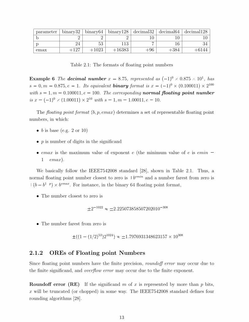
parameter binary32 binary64 binary128 decimal32 decimal64 decimal128b 2 2 2 10 10 10p 24 53 113 7 16 34emax +127 +1023 +16383 +96 +384 +6144
Table 2.1: The formats of floating point numbers
Example 6 The decimal number x 8.75, represented as p1q0 0.875 101, has
s 0, m 0.875, e 1. Its equivalent binary format is x p1q0 p0.100011q 2100
with s 1, m 0.100011, e 100. The corresponding normal floating point number
is x p1q0 p1.00011q 210 with s 1, m 1.00011, e 10.
The floating point format pb, p, emaxq determines a set of representable floating point
numbers, in which:
• b is base (e.g. 2 or 10)
• p is number of digits in the significand
• emax is the maximum value of exponent e (the minimum value of e is emin
1 emaxq.
We basically follow the IEEE7542008 standard [28], shown in Table 2.1. Thus, a
normal floating point number closest to zero is bemin and a number farest from zero is
pb b1pq bemax. For instance, in the binary 64 floating point format,
• The number closest to zero is
21022 2.225073858507202010308
• The number farest from zero is
pp1 p12q53q21024q 1.7976931348623157 10308
2.1.2 OREs of Floating point Numbers
Since floating point numbers have the finite precision, roundoff error may occur due to
the finite significand, and overflow error may occur due to the finite exponent.
Roundoff error (RE) If the significand m of x is represented by more than p bits,
x will be truncated (or chopped) in some way. The IEEE7542008 standard defines four
rounding algorithms [28].
13
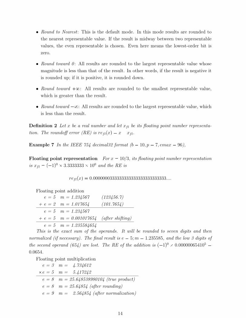
• Round to Nearest : This is the default mode. In this mode results are rounded to
the nearest representable value. If the result is midway between two representable
values, the even representable is chosen. Even here means the lowest-order bit is
zero.
• Round toward 0 : All results are rounded to the largest representable value whose
magnitude is less than that of the result. In other words, if the result is negative it
is rounded up; if it is positive, it is rounded down.
• Round toward 8: All results are rounded to the smallest representable value,
which is greater than the result.
• Round toward 8: All results are rounded to the largest representable value, which
is less than the result.
Definition 2 Let x be a real number and let xfl be its floating point number representa-
tion. The roundoff error (RE) is reflpxq x xfl.
Example 7 In the IEEE 754 decimal32 format (b 10, p 7, emax 96),
Floating point representation For x 103, its floating point number representation
is xfl p1q0 3.3333333 100 and the RE is
reflpxq 0.0000000333333333333333333333333....
Floating point addition
e = 5 m = 1.234567 (123456.7)
+ e = 2 m = 1.017654 (101.7654)
e = 5 m = 1.234567
+ e = 5 m = 0.001017654 (after shifting)
e = 5 m = 1.235584654This is the exact sum of the operands. It will be rounded to seven digits and then
normalized (if necessary). The final result is e 5; m 1.235585, and the low 3 digits of
the second operand (654) are lost. The RE of the addition is p1q0 0.000000654105
0.0654.
Floating point multiplication
e = 3 m = 4.734612
e = 5 m = 5.417242
e = 8 m = 25.648538980104 (true product)
e = 8 m = 25.64854 (after rounding)
e = 9 m = 2.564854 (after normalization)
14
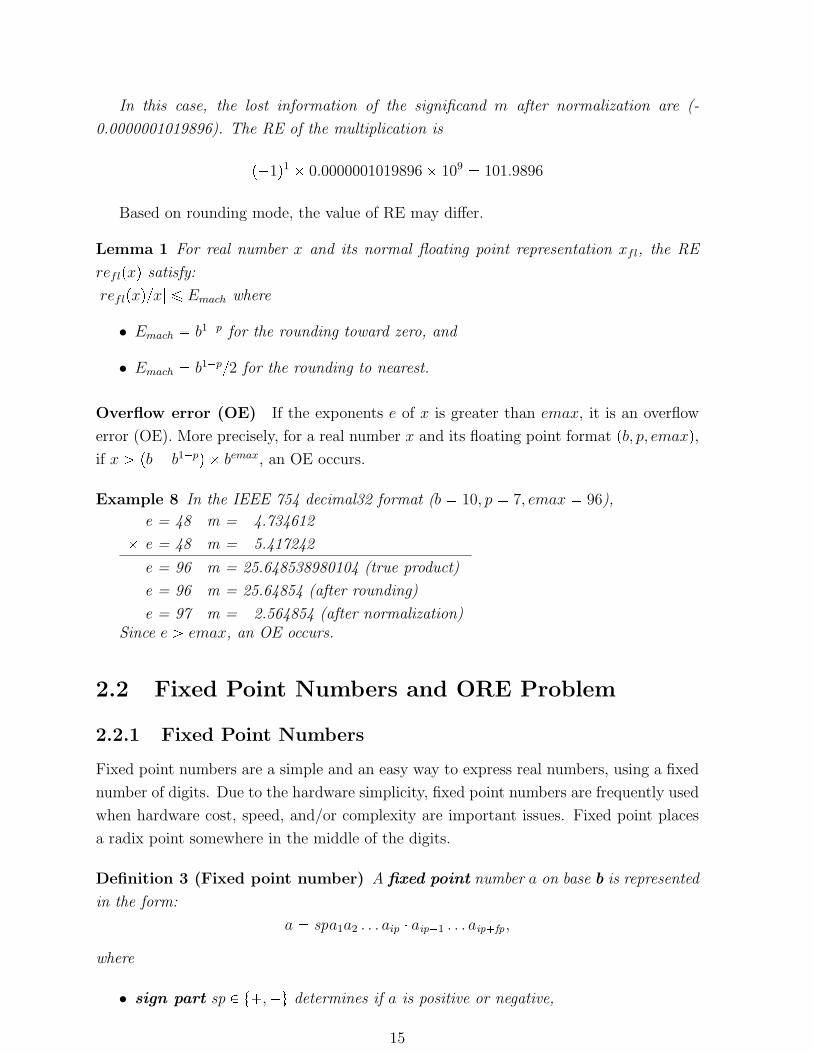
In this case, the lost information of the significand m after normalization are (-
0.0000001019896). The RE of the multiplication is
p1q1 0.0000001019896 109 101.9896
Based on rounding mode, the value of RE may differ.
Lemma 1 For real number x and its normal floating point representation xfl, the RE
reflpxq satisfy:
|reflpxqx| ¤ Emach where
• Emach b1p for the rounding toward zero, and
• Emach b1p2 for the rounding to nearest.
Overflow error (OE) If the exponents e of x is greater than emax, it is an overflow
error (OE). More precisely, for a real number x and its floating point format pb, p, emaxq,
if x ¡ pb b1pq bemax, an OE occurs.
Example 8 In the IEEE 754 decimal32 format (b 10, p 7, emax 96),
e = 48 m = 4.734612
e = 48 m = 5.417242
e = 96 m = 25.648538980104 (true product)
e = 96 m = 25.64854 (after rounding)
e = 97 m = 2.564854 (after normalization)Since e ¡ emax, an OE occurs.
2.2 Fixed Point Numbers and ORE Problem
2.2.1 Fixed Point Numbers
Fixed point numbers are a simple and an easy way to express real numbers, using a fixed
number of digits. Due to the hardware simplicity, fixed point numbers are frequently used
when hardware cost, speed, and/or complexity are important issues. Fixed point places
a radix point somewhere in the middle of the digits.
Definition 3 (Fixed point number) A fixed point number a on base b is represented
in the form:
a spa1a2 . . . aip aip1 . . . aipfp ,
where
• sign part sp P t,u determines if a is positive or negative,
15
• ak P r0, b 1s for each k P r1, ip fps,
• ip is the width of integer part, and
• fp is the width of the fraction part.
The set of fixed point numbers is denoted by Rfx. We omit the sign if it is positive.
In the fixed point format pb, ip, fpq,
• b is base (e.g. 2 or 10).
• ip is number of digits in the integer part.
• fp is number of digits in the fraction part.
Example 9 The number Π is 3.14159 in the fixed point format pb 10, ip 2, fp 5q.
A fixed point number has a fixed window of representation. The range value that can
be represent is pbip 1, bip 1q, and the smallest positive is bfp .
2.2.2 OREs of Fixed point Numbers
Fixed point format is the simple representation of real numbers. The OREs not only occur
when converting real numbers to fixed point number, they also occurs when converting
floating point number to fixed point numbers.
Roundoff error (RE) If the fraction part of number x has more than fp digits, it
needs to truncates to fit the fixed point format. This loses information from digits fp 1
in fraction part, and an RE occurs.
Definition 4 Let x be a real number and let its fixed point number representation be xfx
under the fixed point format pb, ip, fpq. An RE is refxpxq x xfx.
Depending on a rounding mode, the value of RE may differ. For instance, for a real
number x and its fixed point representation xfx, the RE refxpxq satisfies
• |refxpxq| bfp for the round toward zero, and
• |refxpxq| bfp2 for the round to nearest.
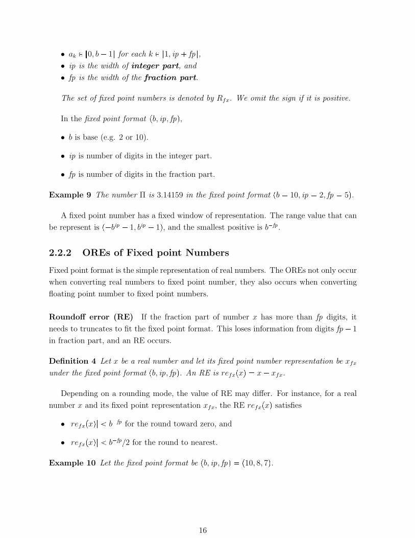
Example 10 Let the fixed point format be pb, ip, fpq p10, 8, 7q.
16
Fixed point representation x 103 is represented as fixed point number xfx
3.3333333. The RE is
refxpxq x xfx 0.0000000333333333333333333333....
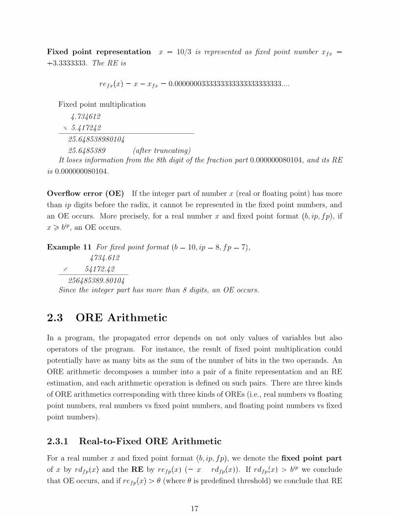
Fixed point multiplication
4.734612
5.417242
25.648538980104
25.6485389 (after truncating)It loses information from the 8th digit of the fraction part 0.000000080104, and its RE
is 0.000000080104.
Overflow error (OE) If the integer part of number x (real or floating point) has more
than ip digits before the radix, it cannot be represented in the fixed point numbers, and
an OE occurs. More precisely, for a real number x and fixed point format pb, ip, fpq, if
x ¥ bip, an OE occurs.
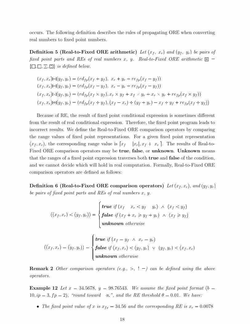
Example 11 For fixed point format pb 10, ip 8, fp 7q,
4734.612
54172.42
256485389.80104Since the integer part has more than 8 digits, an OE occurs.
2.3 ORE Arithmetic
In a program, the propagated error depends on not only values of variables but also
operators of the program. For instance, the result of fixed point multiplication could
potentially have as many bits as the sum of the number of bits in the two operands. An
ORE arithmetic decomposes a number into a pair of a finite representation and an RE
estimation, and each arithmetic operation is defined on such pairs. There are three kinds
of ORE arithmetics corresponding with three kinds of OREs (i.e., real numbers vs floating
point numbers, real numbers vs fixed point numbers, and floating point numbers vs fixed
point numbers).
2.3.1 Real-to-Fixed ORE Arithmetic
For a real number x and fixed point format pb, ip, fpq, we denote the fixed point part
of x by rdfppxq and the RE by refppxq ( x rdfppxq). If rdfppxq ¡ bip we conclude
that OE occurs, and if refppxq ¡ θ (where θ is predefined threshold) we conclude that RE
17
occurs. The following definition describes the rules of propagating ORE when converting
real numbers to fixed point numbers.
Definition 5 (Real-to-Fixed ORE arithmetic) Let pxf , xrq and pyf , yrq be pairs of
fixed point parts and REs of real numbers x, y. Real-to-Fixed ORE arithmetic f
t`,a,b,cu is defined below.
pxf , xrq`pyf , yrq prdfppxf yf q, xr yr refppxf yf qq
pxf , xrqapyf , yrq prdfppxf yf q, xr yr refppxf yf qq
pxf , xrqbpyf , yrq prdfppxf yf q, xr yf xf yr xr yr refppxf yf qq
pxf , xrqcpyf , yrq prdfppxf yf q, pxf xrq pyf yrq xf yf refppxf yf qq
Because of RE, the result of fixed point conditional expression is sometimes different
from the result of real conditional expression. Therefore, the fixed point program leads to
incorrect results. We define the Real-to-Fixed ORE comparison operators by comparing
the range values of fixed point representations. For a given fixed point representation
pxf , xrq, the corresponding range value is rxf |xr|, xf |xr|s. The results of Real-to-
Fixed ORE comparison operators may be true, false, or unknown. Unknown means
that the ranges of a fixed point expression traverses both true and false of the condition,
and we cannot decide which will hold in real computation. Formally, Real-to-Fixed ORE
comparison operators are defined as follows:
Definition 6 (Real-to-Fixed ORE comparison operators) Let pxf , xrq, and pyf , yrq
be pairs of fixed point parts and REs of real numbers x, y.
ppxf , xrq pyf , yrqq
$'''&'''%true if pxf xr yf yrq ^ pxf yf q
false if pxf xr ¥ yf yrq ^ pxf ¥ yf q
unknown otherwise
ppxf , xrq pyf , yrqq
$'''&'''%true if pxf yf ^ xr yrq
false if pxf , xrq pyf , yrq _ pyf , yrq pxf , xrq
unknown otherwise
Remark 2 Other comparison operators (e.g., ¡, ! ) can be defined using the above
operators.
Example 12 Let x 34.5678, y 98.76543. We assume the fixed point format pb
10, ip 3, fp 2q, “round toward 8”, and the RE threshold θ 0.01. We have:
• The fixed point value of x is xfx 34.56 and the corresponding RE is xr 0.0078
18
• The fixed point value of y is yfx 98.76 and the corresponding RE is yr 0.00543
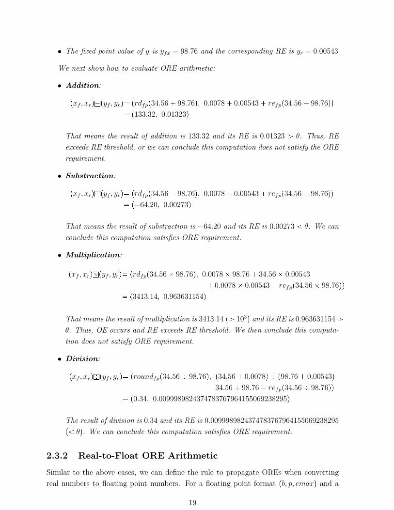
We next show how to evaluate ORE arithmetic:
• Addition:
pxf , xrq`pyf , yrq prdfpp34.56 98.76q, 0.0078 0.00543 refpp34.56 98.76qq
p133.32, 0.01323q
That means the result of addition is 133.32 and its RE is 0.01323 ¡ θ. Thus, RE
exceeds RE threshold, or we can conclude this computation does not satisfy the ORE
requirement.
• Substraction:
pxf , xrqapyf , yrq prdfpp34.56 98.76q, 0.0078 0.00543 refpp34.56 98.76qq
p64.20, 0.00273q
That means the result of substraction is 64.20 and its RE is 0.00273 θ. We can
conclude this computation satisfies ORE requirement.
• Multiplication:
pxf , xrqbpyf , yrq prdfpp34.56 98.76q, 0.0078 98.76 34.56 0.00543
0.0078 0.00543 refpp34.56 98.76qq
p3413.14, 0.963631154q
That means the result of multiplication is 3413.14 p¡ 103q and its RE is 0.963631154 ¡
θ. Thus, OE occurs and RE exceeds RE threshold. We then conclude this computa-
tion does not satisfy ORE requirement.
• Division:
pxf , xrqcpyf , yrq proundfpp34.56 98.76q, p34.56 0.0078q p98.76 0.00543q
34.56 98.76 refpp34.56 98.76qq
p0.34, 0.0099989824374783767964155069238295q
The result of division is 0.34 and its RE is 0.0099989824374783767964155069238295
p θq. We can conclude this computation satisfies ORE requirement.
2.3.2 Real-to-Float ORE Arithmetic
Similar to the above cases, we can define the rule to propagate OREs when converting
real numbers to floating point numbers. For a floating point format pb, p, emaxq and a
19
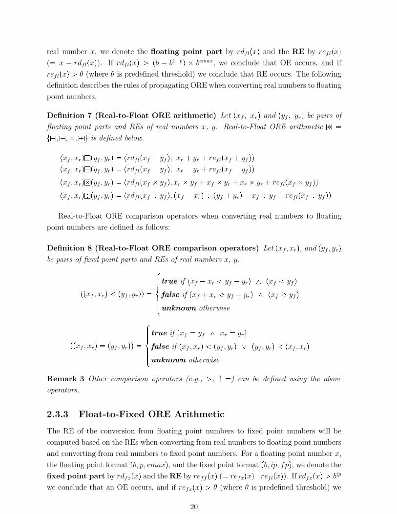
real number x, we denote the floating point part by rdflpxq and the RE by reflpxq
( x rdflpxq). If rdflpxq ¡ pb b1pq bemax, we conclude that OE occurs, and if
reflpxq ¡ θ (where θ is predefined threshold) we conclude that RE occurs. The following
definition describes the rules of propagating ORE when converting real numbers to floating
point numbers.
Definition 7 (Real-to-Float ORE arithmetic) Let pxf , xrq and pyf , yrq be pairs of
floating point parts and REs of real numbers x, y. Real-to-Float ORE arithmetic f
t`,a,b,cu is defined below.
pxf , xrq`pyf , yrq prdflpxf yf q, xr yr reflpxf yf qq
pxf , xrqapyf , yrq prdflpxf yf q, xr yr reflpxf yf qq
pxf , xrqbpyf , yrq prdflpxf yf q, xr yf xf yr xr yr reflpxf yf qq
pxf , xrqcpyf , yrq prdflpxf yf q, pxf xrq pyf yrq xf yf reflpxf yf qq
Real-to-Float ORE comparison operators when converting real numbers to floating
point numbers are defined as follows:
Definition 8 (Real-to-Float ORE comparison operators) Let pxf , xrq, and pyf , yrq
be pairs of fixed point parts and REs of real numbers x, y.
ppxf , xrq pyf , yrqq
$'''&'''%true if pxf xr yf yrq ^ pxf yf q
false if pxf xr ¥ yf yrq ^ pxf ¥ yf q
unknown otherwise
ppxf , xrq pyf , yrqq
$'''&'''%true if pxf yf ^ xr yrq
false if pxf , xrq pyf , yrq _ pyf , yrq pxf , xrq
unknown otherwise
Remark 3 Other comparison operators (e.g., ¡, ! ) can be defined using the above
operators.
2.3.3 Float-to-Fixed ORE Arithmetic
The RE of the conversion from floating point numbers to fixed point numbers will be
computed based on the REs when converting from real numbers to floating point numbers
and converting from real numbers to fixed point numbers. For a floating point number x,
the floating point format pb, p, emaxq, and the fixed point format pb, ip, fpq, we denote the
fixed point part by rdfxpxq and the RE by reff pxq ( refxpxqreflpxq). If rdfxpxq ¡ bip
we conclude that an OE occurs, and if refxpxq ¡ θ (where θ is predefined threshold) we
20
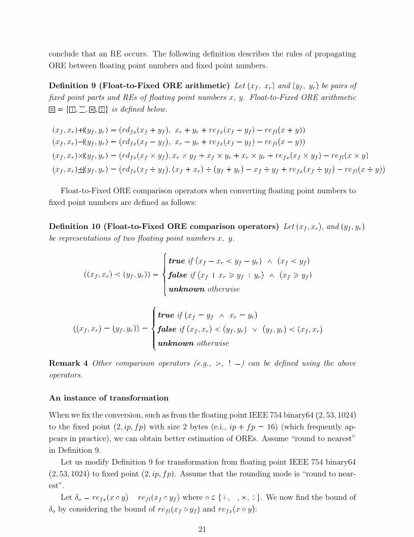
conclude that an RE occurs. The following definition describes the rules of propagating
ORE between floating point numbers and fixed point numbers.
Definition 9 (Float-to-Fixed ORE arithmetic) Let pxf , xrq and pyf , yrq be pairs of
fixed point parts and REs of floating point numbers x, y. Float-to-Fixed ORE arithmetic
f t`,a,b,cu is defined below.
pxf , xrq`pyf , yrq prdfxpxf yf q, xr yr refxpxf yf q reflpx yqq
pxf , xrqapyf , yrq prdfxpxf yf q, xr yr refxpxf yf q reflpx yqq
pxf , xrqbpyf , yrq prdfxpxf yf q, xr yf xf yr xr yr refxpxf yf q reflpx yq
pxf , xrqcpyf , yrq prdfxpxf yf q, pxf xrq pyf yrq xf yf refxpxf yf q reflpx yqq
Float-to-Fixed ORE comparison operators when converting floating point numbers to
fixed point numbers are defined as follows:
Definition 10 (Float-to-Fixed ORE comparison operators) Let pxf , xrq, and pyf , yrq
be representations of two floating point numbers x, y.
ppxf , xrq pyf , yrqq
$'''&'''%true if pxf xr yf yrq ^ pxf yf q
false if pxf xr ¥ yf yrq ^ pxf ¥ yf q
unknown otherwise
ppxf , xrq pyf , yrqq
$'''&'''%true if pxf yf ^ xr yrq
false if pxf , xrq pyf , yrq _ pyf , yrq pxf , xrq
unknown otherwise
Remark 4 Other comparison operators (e.g., ¡, ! ) can be defined using the above
operators.
An instance of transformation
When we fix the conversion, such as from the floating point IEEE 754 binary64 p2, 53, 1024q
to the fixed point p2, ip, fpq with size 2 bytes (e.i., ip fp 16) (which frequently ap-
pears in practice), we can obtain better estimation of OREs. Assume “round to nearest”
in Definition 9.
Let us modify Definition 9 for transformation from floating point IEEE 754 binary64
p2, 53, 1024q to fixed point p2, ip, fpq. Assume that the rounding mode is “round to near-
est”.
Let δ refxpx yq reflpxf yf q where P t,,,u. We now find the bound of
δ by considering the bound of reflpxf yf q and refxpx yq:
21
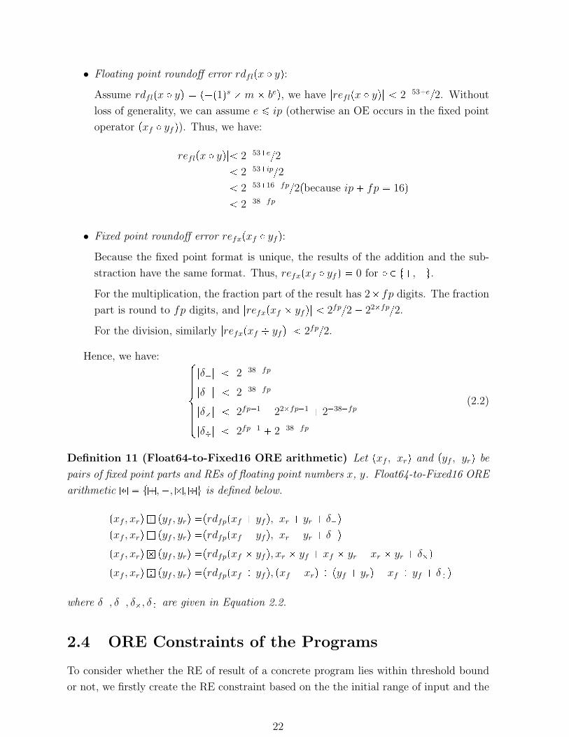
• Floating point roundoff error rdflpx yq:
Assume rdflpx yq pp1qs m beq, we have |reflpx yq| 253e2. Without
loss of generality, we can assume e ¤ ip (otherwise an OE occurs in the fixed point
operator pxf yf q). Thus, we have:
|reflpx yq| 253e2
253ip2
25316fp2pbecause ip fp 16q
238fp
• Fixed point roundoff error refxpxf yf q:
Because the fixed point format is unique, the results of the addition and the sub-
straction have the same format. Thus, refxpxf yf q 0 for P t,u.
For the multiplication, the fraction part of the result has 2fp digits. The fraction
part is round to fp digits, and |refxpxf yf q| 2fp2 22fp2.
For the division, similarly |refxpxf yf q| 2fp2.
Hence, we have: $'''''&'''''%|δ| 238fp
|δ| 238fp
|δ| 2fp1 22fp1 238fp
|δ| 2fp1 238fp
(2.2)
Definition 11 (Float64-to-Fixed16 ORE arithmetic) Let pxf , xrq and pyf , yrq be
pairs of fixed point parts and REs of floating point numbers x, y. Float64-to-Fixed16 ORE
arithmetic f t`,a,b,cu is defined below.
pxf , xrq` pyf , yrq prdfppxf yf q, xr yr δq
pxf , xrqa pyf , yrq prdfppxf yf q, xr yr δq
pxf , xrqb pyf , yrq prdfppxf yf q, xr yf xf yr xr yr δq
pxf , xrqc pyf , yrq prdfppxf yf q, pxf xrq pyf yrq xf yf δq
where δ, δ, δ, δ are given in Equation 2.2.
2.4 ORE Constraints of the Programs
To consider whether the RE of result of a concrete program lies within threshold bound
or not, we firstly create the RE constraint based on the the initial range of input and the
22
threshold bound of RE. Next, we need to solve the RE constraint to clarify whether the
RE occur or not.
A sample program language
A general program basically includes three types of instructions: assignments, conditions,
and loops. This program language does not contain exception, recursive function and
pointers.
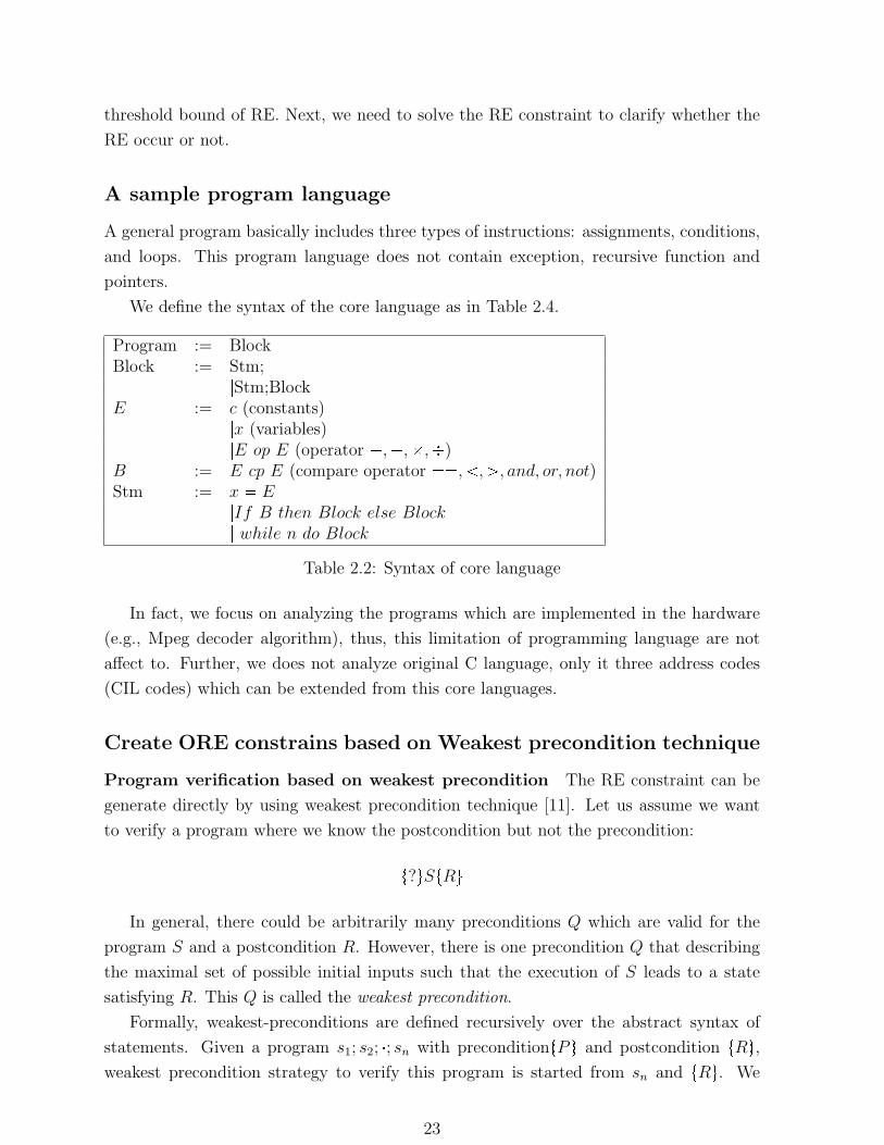
We define the syntax of the core language as in Table 2.4.
Program := BlockBlock := Stm;
|Stm;BlockE := c (constants)
|x (variables)|E op E (operator ,,,)
B := E cp E (compare operator , ,¡, and, or, not)Stm := x E
|If B then Block else Block| while n do Block
Table 2.2: Syntax of core language
In fact, we focus on analyzing the programs which are implemented in the hardware
(e.g., Mpeg decoder algorithm), thus, this limitation of programming language are not
affect to. Further, we does not analyze original C language, only it three address codes
(CIL codes) which can be extended from this core languages.
Create ORE constrains based on Weakest precondition technique
Program verification based on weakest precondition The RE constraint can be
generate directly by using weakest precondition technique [11]. Let us assume we want
to verify a program where we know the postcondition but not the precondition:
t?uStRu
In general, there could be arbitrarily many preconditions Q which are valid for the
program S and a postcondition R. However, there is one precondition Q that describing
the maximal set of possible initial inputs such that the execution of S leads to a state
satisfying R. This Q is called the weakest precondition.
Formally, weakest-preconditions are defined recursively over the abstract syntax of
statements. Given a program s1; s2; ; sn with preconditiontP u and postcondition tRu,
weakest precondition strategy to verify this program is started from sn and tRu. We
23
produce tPn1u is the weakest precondition for the statement sn. tPn1u now becomes
the postcondition for sn1. Then we continue produce tPn2u is weakest precondition of
sn1.
tP us1; s 2; ; sntRu
tP u
tP0u
ts1u
tP1u
tsn1u
tRu
Doing similarly, we obtain P0 finally. What remains is to prove
P ñ P0
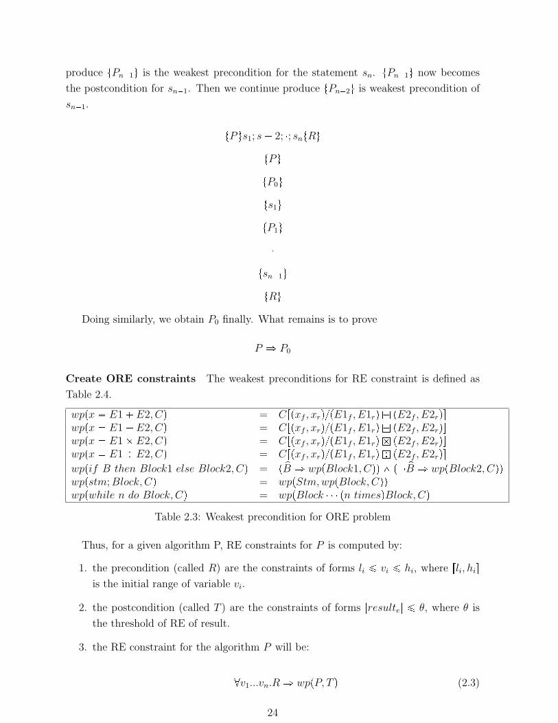
Create ORE constraints The weakest preconditions for RE constraint is defined as
Table 2.4.
wppx E1 E2, Cq = Crpxf , xrqpE1f , E1rq` pE2f , E2rqswppx E1 E2, Cq = Crpxf , xrqpE1f , E1rqa pE2f , E2rqswppx E1 E2, Cq = Crpxf , xrqpE1f , E1rqb pE2f , E2rqswppx E1 E2, Cq = Crpxf , xrqpE1f , E1rqc pE2f , E2rqs
wppif B then Block1 else Block2, Cq = p pB ñ wppBlock1, Cqq ^ p pB ñ wppBlock2, Cqqwppstm; Block, Cq = wppStm, wppBlock, Cqqwppwhile n do Block, Cq = wppBlock pn timesqBlock, Cq
Table 2.3: Weakest precondition for ORE problem
Thus, for a given algorithm P, RE constraints for P is computed by:
1. the precondition (called R) are the constraints of forms li ¤ vi ¤ hi, where rli, his
is the initial range of variable vi.
2. the postcondition (called T ) are the constraints of forms |resulte| ¤ θ, where θ is
the threshold of RE of result.
3. the RE constraint for the algorithm P will be:
@v1...vn.R ñ wppP, T q (2.3)
24
If 2.3 is true then the RE value is acceptable. Otherwise, there is a input that makes
the RE value too large. The problem now is how to verify the constraint (2.3).
Solving ORE constraint problem
We consider the case: the fixed point part is fixed, and the RE part is changeable. We
have an observation that, even with this simple case, it will be reduced to polynomial
inequations over real. Brown [6] shows that the quantifier elimination of polynomial in-
equations over real are double exponential. Therefore, the problem of solving requires
doubly exponential time complexity. As a consequence, finding exactly ORE is impracti-
cal.
25
Chapter 3
Dataflow Analysis as Weighted
Model Checking
It has been suggested intimate connections between dataflow analysis and model check-
ing [48, 57]. A program is firstly encoded into a model (transition system) by abstraction,
and a program analysis is formulated as a model checking problem. This is nicely adopted
for control flow analysis and/or classical dataflow analysis in Dragon book [1, 35]. How-
ever, as natural requests, we intend more richer dataflow, such as quantity properties
with more precise treatments on conditional branches. For instance, linear constraint
propagation [48], affine relation analysis [56], or ORE constraint analysis [51] are such
examples. In these cases, the direct encoding will be a-transition-as-an-environment-
transformer, which requires all possible environments as states. This will lead the state
explosion problem in model checking. In 2003, Rep [55] proposed weighted pushdown
model checking, in which each transition is associated with a weight. A weight directly
represents dataflow, that is, how an abstract environment will be transformed, without
generating explicit environments as states. This will not improve complexity in theory,
but in practice we can combine with an on-the-fly generation of weights, which drastically
reduces the search space during model checking. We follow this weighted model check-
ing approach (but without using a pushdown stack). In this chapter, we briefly describe
how to transform dataflow analysis problem as a model checking problem and abstraction
(Section 3.1). We then describe the idea of transforming dataflow analysis problem to
weighted model checking problem and abstraction in Section 3.2.
26
3.1 Dataflow Analysis as Model Checking and Ab-
straction
3.1.1 Dataflow Analysis
Dataflow analysis [50] is a special case of program analysis which statically computes
information about the flow of data for each program point. This information must be
a safe approximation of the desired properties of the run-time behavior of the program
during each possible execution of that program for all possible inputs. In general, there
are 3 common approach for solving dataflow analysis problem:
• Constraint resolution systems: consist of a constraint store and a logic for solving
constraints. In particular, a program component constraints the semantic prop-
erties. These constraints are expressed in form of inequalities and the semantics
properties are derived by finding a solution which satisfies all the constraints. In
this approach, SAT/SMT solver can be used to help solving the constraints [19].
• Model checking: the classical dataflow analysis can be transformed to model checking
problem by creating suitable abstractions of the programs as models and expressing
desired properties in terms of boolean formulae. A model checking algorithm then
discovers the states in the model that satisfy the given formulae.
• Abstract interpretations use abstraction functions to map the concrete semantic
values to abstract semantics, perform the computations on the abstract semantics,
and use concretization functions to map the abstract semantics back to the concrete
semantic.
Dataflow analysis can be characterized by the following properties:
• Context sensitive: analysis is an interprocedural analysis that considers the calling
context when analyzing the target of a function call. In particular, using context
information one can jump back to the original call site, whereas without that infor-
mation, the analysis information has to be propagated back to all possible call sites,
potentially losing precision. In general, fully context sensitive analysis is very inef-
ficient and most practical algorithms employ a limited amount of context sensitive.
• Flow sensitive: analysis takes into account the order of statements in a program. For
example, a flow-insensitive pointer alias analysis may determine “variables x and
y may refer to the same location”, while a flow-sensitive analysis may determine
“after statement 20, variables x and y may refer to the same location”.
• Path sensitive: analysis computes different pieces of analysis information dependent
on the predicates at conditional branch instructions. For instance, if a branch
27
contains a condition x¿0, then on the fall-through path, the analysis would assume
that x¡=0 and on the target of the branch it would assume that indeed x¿0 holds.
Basically, the representations of dataflow are sets of program entities such as variables
or expressions satisfying the given property. The classical dataflow analysis [1](e.g., live-
variable, partial-redundancy elimination) implements these sets by bit-vectors. However,
the new dataflow analysis problems [25, 51](e.g., linear constraint, affine relation) may
need extra information about value of variables, hence these sets must be implemented
by non-bit-vectors.
Dataflow analysis is used to: (1) determining the semantic validity of a program (e.g.,
type correctness); (2) understanding the behavior of a program for debugging, verification,
testing [25, 51]; (3) transforming a program for optimized the program for space, time, or
power consumption [24].
3.1.2 Model Checking
Model checking, proposed independently by E.M. Clarke and E.A. Emerson (USA) and
J.Sifakis (France) in 1980 [7], is an automatic verification technique for finite state con-
current systems. The model checking problem is:
Given a program (system model) M and a correctness specification S, deter-
mine whether or not the behavior of M satisfies the specification B?.
Applying model checking to a system consists of two main tasks:
Specifying the properties that system should have, for example, deadlock, divergence
or deadlock. The specification is usually given in some logical formalism. For hardware
and software systems, it is common to use temporal logic [12], which can assert how the
behavior of the system evolves over time, such as CTL (computation tree logic) and LTL
(linear time logic). An important issue in specification is completeness. Model checking
provides means for checking that a model of the design satisfies a given specification, but
it is impossible to determine whether the given specification covers all the properties that
the system should satisfy.
Construct a formal model for the system. In many cases, this is simply a compilation
task. In other cases, the modeling of a design may require the use of abstraction to
eliminate irrelevant of unimportant details. For example, when modeling programs for
checking ORE, we it is useful to consider numerical variables, rather than string variables.
28
Model checker
Systemmodel
Systemproperties
Property fulfilled?
yes
Notification
no
Counter-examples
Figure 3.1: Model checker structure
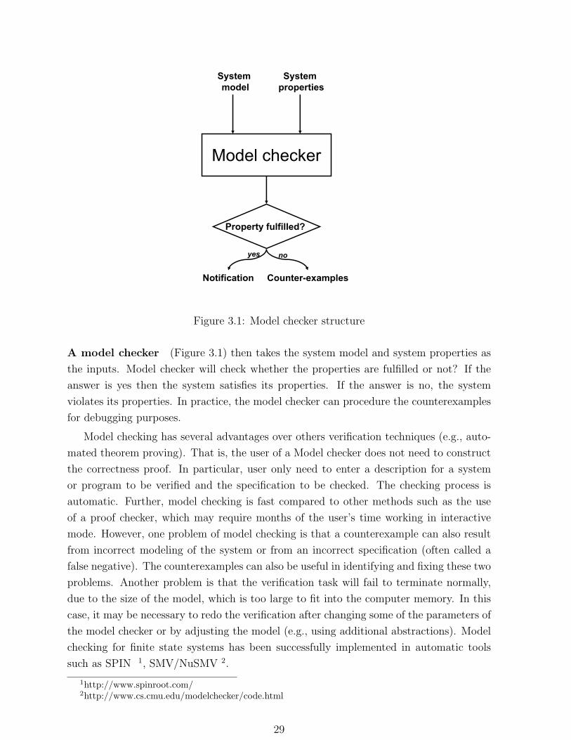
A model checker (Figure 3.1) then takes the system model and system properties as
the inputs. Model checker will check whether the properties are fulfilled or not? If the
answer is yes then the system satisfies its properties. If the answer is no, the system
violates its properties. In practice, the model checker can procedure the counterexamples
for debugging purposes.
Model checking has several advantages over others verification techniques (e.g., auto-
mated theorem proving). That is, the user of a Model checker does not need to construct
the correctness proof. In particular, user only need to enter a description for a system
or program to be verified and the specification to be checked. The checking process is
automatic. Further, model checking is fast compared to other methods such as the use
of a proof checker, which may require months of the user’s time working in interactive
mode. However, one problem of model checking is that a counterexample can also result
from incorrect modeling of the system or from an incorrect specification (often called a
false negative). The counterexamples can also be useful in identifying and fixing these two
problems. Another problem is that the verification task will fail to terminate normally,
due to the size of the model, which is too large to fit into the computer memory. In this
case, it may be necessary to redo the verification after changing some of the parameters of
the model checker or by adjusting the model (e.g., using additional abstractions). Model
checking for finite state systems has been successfully implemented in automatic tools
such as SPIN 1, SMV/NuSMV 2.
1http://www.spinroot.com/2http://www.cs.cmu.edu/modelchecker/code.html
29
3.1.3 Dataflow Analysis as Model Checking and Abstraction
As we known, the classical dataflow analysis can be transformed to model checking prob-
lem by creating suitable abstractions of the programs as models and expressing desired
properties in terms of temporal formulae (e.g., CTL formulae) [34].
Modeling program Given a program, the standard program model includes:
• program states are the program locals (e.g., program point),
• actions are the elementary statements and expressions, and
• transitions are defined by the small steps and are labeled with corresponding prim-
itive statements/expressions.
The programs can be modeled as labeled transition systems.
Definition 12 A label transition system P is a tuple pS, A, ∆q in which
• S is a finite set of nodes or program states,
• A is a set of actions, modeling elementary statements,
• ∆ S A S is a set of labeled transitions, which modeling the flow of control,
and
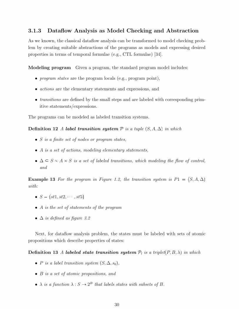
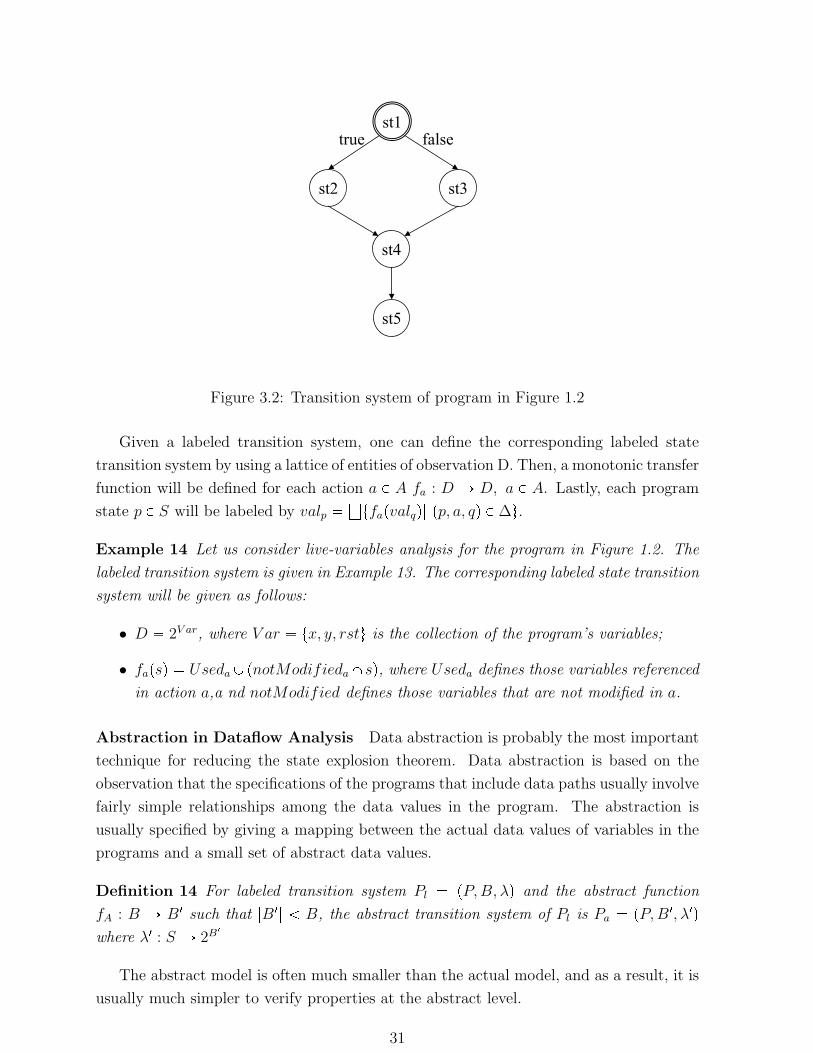
Example 13 For the program in Figure 1.2, the transition system is P1 pS, A, ∆q
with:
• S tst1, st2, , st5u
• A is the set of statements of the program
• ∆ is defined as figure 3.2
Next, for dataflow analysis problem, the states must be labeled with sets of atomic
propositions which describe properties of states:
Definition 13 A labeled state transition system Pl is a tripletpP, B, λq in which
• P is a label transition system pS, ∆, s0q,
• B is a set of atomic propositions, and
• λ is a function λ : S Ñ 2B that labels states with subsets of B.
30
st5
st1
st2 st3
st4
true false
Figure 3.2: Transition system of program in Figure 1.2
Given a labeled transition system, one can define the corresponding labeled state
transition system by using a lattice of entities of observation D. Then, a monotonic transfer
function will be defined for each action a P A fa : D Ñ D, a P A. Lastly, each program
state p P S will be labeled by valp tfapvalqq| pp, a, qq P ∆u.
Example 14 Let us consider live-variables analysis for the program in Figure 1.2. The
labeled transition system is given in Example 13. The corresponding labeled state transition
system will be given as follows:
• D 2V ar, where V ar tx, y, rstu is the collection of the program’s variables;
• fapsq UsedaYpnotModifiedaXsq, where Useda defines those variables referenced
in action a,a nd notModified defines those variables that are not modified in a.
Abstraction in Dataflow Analysis Data abstraction is probably the most important
technique for reducing the state explosion theorem. Data abstraction is based on the
observation that the specifications of the programs that include data paths usually involve
fairly simple relationships among the data values in the program. The abstraction is
usually specified by giving a mapping between the actual data values of variables in the
programs and a small set of abstract data values.
Definition 14 For labeled transition system Pl pP, B, λq and the abstract function
fA : B Ñ B1 such that |B1| B, the abstract transition system of Pl is Pa pP, B1, λ1q
where λ1 : S Ñ 2B1
The abstract model is often much smaller than the actual model, and as a result, it is
usually much simpler to verify properties at the abstract level.
31
Example 15 For the program in Figure 1.2, assume that the initial values of variable
x, y lie in t1, 1, 3u. We would like to check whether the result of rst is even or odd.
The transition system P1 is already given in Example 13. Directly, we can set the
states of the transition system P1 in example are all possible values of x, y, rst. Hence,
B t1, 0, 1, 2, 3, 4, 9, ...u. However, we can safety abstract B to B1 teven, oddu where
fApxq even if x div 2, fApxq odd otherwise. By this, the abstract model will become
simpler than the concrete model.
Source program + abstraction of input data
Finite program model:• arcs labelled
by program actions
Finite program model:• arcs labelled
by abstract actions• node labelled
by abstract states
static analysis result
Model checking
Abstraction
Pre-processing
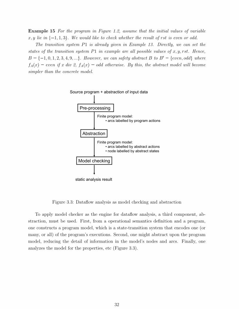
Figure 3.3: Dataflow analysis as model checking and abstraction
To apply model checker as the engine for dataflow analysis, a third component, ab-
straction, must be used. First, from a operational semantics definition and a program,
one constructs a program model, which is a state-transition system that encodes one (or
many, or all) of the program’s executions. Second, one might abstract upon the program
model, reducing the detail of information in the model’s nodes and arcs. Finally, one
analyzes the model for the properties, etc (Figure 3.3).
32
3.2 Dataflow Analysis as Weighted Model Checking
Problem
3.2.1 Weighted Model Checking
Weighted model checking (WMC) computes dataflow (or, an update of environments)
by associating a weight to each transition in the model, and the goal is to determine the
weight summary of the meet-over-all-path. In one hand, the computation of fixpoint often
require widening operation that causes over approximation too much (e.g., approximate
value of variable to 8). In other hand, the most important requirement of ORE analysis
is precision. Thus, in order to avoiding widening operation, we restrict the underlying
pushdown system to a finite state transition system. By this, the weighted pushdown
model checking becomes weighted model checking.
Weight domain and weighted transition system. In weighted model checking, the
weight domain D is an idempotent semiring.
Definition 15 An idempotent semiring is a quintuple pD,`,b,0,1q, where 0,1 P D
and `, b are binary operators on D such that, for a, b, c P D,
• pD,`q is a commutative monoid with the unit 0,
• pD,bq is a monoid with the unit 1,
• b distributes over `, i.e., abpb`cq pabbq`pabcq and pa`bqbc pabcq`pbbcq,
• ` is idempotent, i.e., a` a a, and
• 0 is the zero element of b, i.e., ab 0 0b a 0.
In the context of dataflow analysis, each element of an idempotent semiring is regarded
as follows:
• 0 stands for interruption of dataflow,
• 1 stands for the identity function (i.e., no state update),
• b is the composition of two successive dataflow, and
• ` merges two dataflow at the meet of two transition sequences.
The weighted transition system is then defined as a transition system “plus” a weight
domain.
33
Definition 16 Let P pP, ∆, s0q be a transition system with P to be a finite set of states,
∆p P P q to be a set of transitions, and s0pP P q to be an initial state. A weighted
transition system (WTS) is a triplet W pP , S, fq, where S pD,`,b,0,1q is an
idempotent semiring and f : ∆ Ñ D is a map that assigns a weight to each transition.
Let ∆ be the set of all sequences of transitions. For σ rr1, . . . , rks P ∆, we
define vpσq ∆ fpr1q b . . .b fprkq. If σ is a transition sequence from a state c to a state
c1, we denote c ñσ c1. The set of all such sequences is denoted by pathspc, c1q, i.e.,
pathspc, c1q tσ | c ñσ c1u
Weighted model checking. Weighted model checking finds the weight summary of
pathspc, c1q, which is the summation `σPpathspc,c1qvpσq.
There are two kinds of generalized reachability problems:
Definition 17 Let W pP ,S, fq be a weighted transition system with P pP, ∆, s0q.
Let C P and c P P .
• The generalized predecessor problem is to find δpcq `tvpσq | σ P pathpc, c1q, c1 P
Cu.
• The generalized successor problem is to find δpcq `tvpσq | σ P pathpc1, cq, c1 P
Cu
If a cycle exists in a weighted model, pathspc, c1q becomes infinite. For the termination
of a weighted model checking, an idempotent semiring needs to be bounded.
Definition 18 An idempotent semiring is bounded if there are no infinite descending
chains wrt , where a b if, and only if, a` b a.
Data Abstraction and Weight Domain
For the purpose of dataflow analysis, the weights capture the relationships between the
values of variables before and after the statements. Thus, the weight domain can be
treated as a set of abstract transformers.
More formally, let V, V be the set of variables and the set of their corresponding values,
respectively. The abstract function is fA : V Ñ VA where VA is abstract domain of V.
Hence, the weight domain D is the set of functions f : VA Ñ VA which stands for the
transformations from abstract values of variables before statements to the abstract values
of variables after statements.
34
3.2.2 Dataflow Analysis as Weighted Model Checking and Ab-
straction
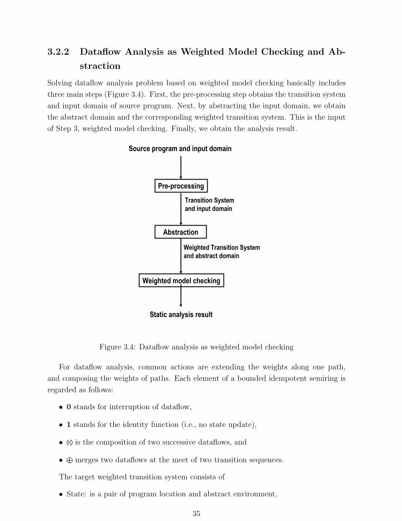
Solving dataflow analysis problem based on weighted model checking basically includes
three main steps (Figure 3.4). First, the pre-processing step obtains the transition system
and input domain of source program. Next, by abstracting the input domain, we obtain
the abstract domain and the corresponding weighted transition system. This is the input
of Step 3, weighted model checking. Finally, we obtain the analysis result.
Source program and input domain
Static analysis result
Weighted model checking
Pre-processing
Transition System and input domain
Weighted Transition System and abstract domain
Abstraction
Figure 3.4: Dataflow analysis as weighted model checking
For dataflow analysis, common actions are extending the weights along one path,
and composing the weights of paths. Each element of a bounded idempotent semiring is
regarded as follows:
• 0 stands for interruption of dataflow,
• 1 stands for the identity function (i.e., no state update),
• b is the composition of two successive dataflows, and
• ` merges two dataflows at the meet of two transition sequences.
The target weighted transition system consists of
• State: is a pair of program location and abstract environment,
35
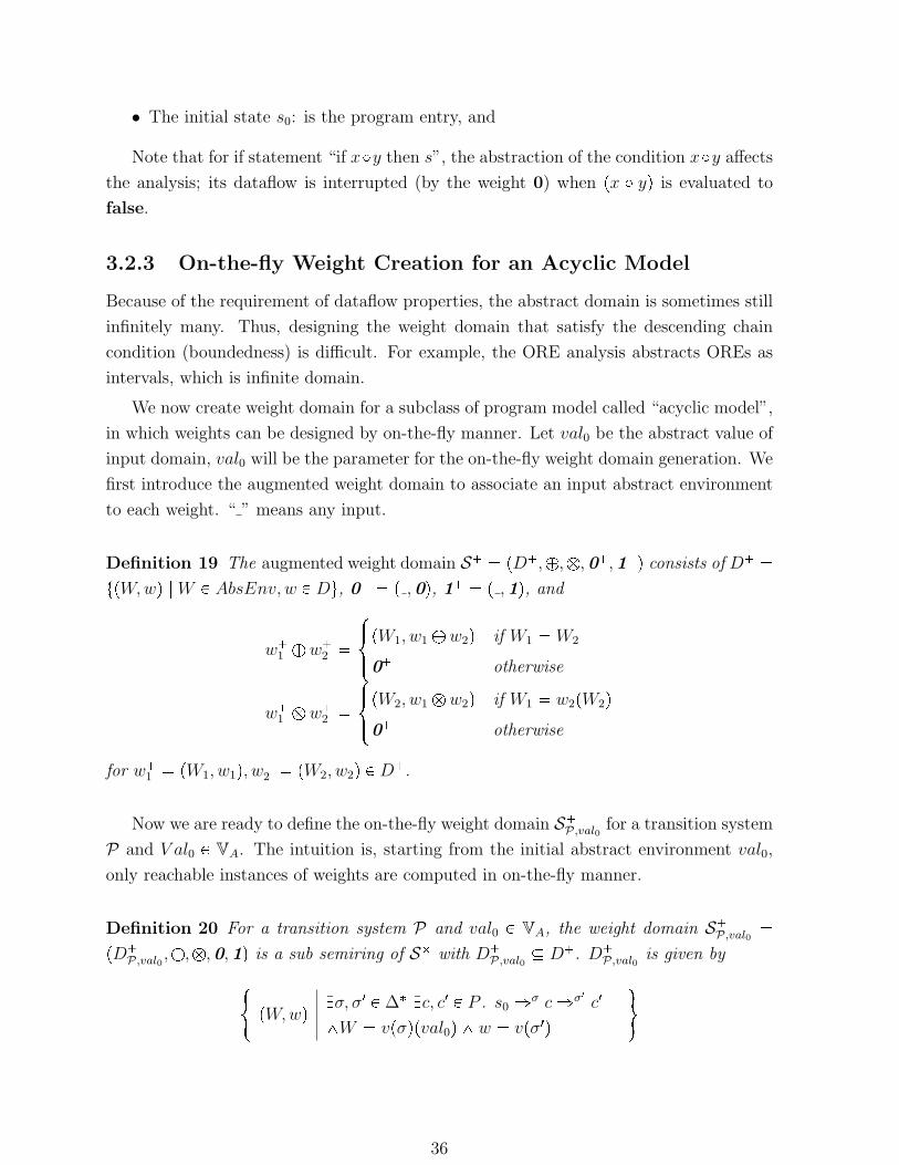
• The initial state s0: is the program entry, and
Note that for if statement “if xy then s”, the abstraction of the condition xy affects
the analysis; its dataflow is interrupted (by the weight 0) when px yq is evaluated to
false.
3.2.3 On-the-fly Weight Creation for an Acyclic Model
Because of the requirement of dataflow properties, the abstract domain is sometimes still
infinitely many. Thus, designing the weight domain that satisfy the descending chain
condition (boundedness) is difficult. For example, the ORE analysis abstracts OREs as
intervals, which is infinite domain.
We now create weight domain for a subclass of program model called “acyclic model”,
in which weights can be designed by on-the-fly manner. Let val0 be the abstract value of
input domain, val0 will be the parameter for the on-the-fly weight domain generation. We
first introduce the augmented weight domain to associate an input abstract environment
to each weight. “ ” means any input.
Definition 19 The augmented weight domain S pD,`,b,0,1q consists of D
tpW, wq | W P AbsEnv, w P Du, 0 p ,0q, 1 p ,1q, and
w1 ` w
2
$&%pW1, w1 ` w2q if W1 W2
0 otherwise
w1 b w
2
$&%pW2, w1 b w2q if W1 w2pW2q
0 otherwise
for w1 pW1, w1q, w
2 pW2, w2q P D.
Now we are ready to define the on-the-fly weight domain SP,val0
for a transition system
P and V al0 P VA. The intuition is, starting from the initial abstract environment val0,
only reachable instances of weights are computed in on-the-fly manner.
Definition 20 For a transition system P and val0 P VA, the weight domain SP,val0
pDP,val0
,`,b,0,1q is a sub semiring of S with DP,val0
D. DP,val0
is given by#pW, wq
Dσ, σ1 P ∆ Dc, c1 P P . s0 ñσ c ñσ1 c1
^W vpσqpval0q ^ w vpσ1q
+
36
Chapter 4
Interval Arithmetics in ORE
Propagation
In general, we do not know the exact values of variables in the program, only their
ranges. Hence, estimating ORE can be solved by propagating fixed point ranges and
round off error ranges of variables. In order to estimate OREs of operations, there are
two known range representations: classical interval [47] and affine interval [61, 62]. In
this chapter, we firstly describe these two methods in detail in Sections 4.1 and 4.2.
Then, motivated by the disadvantages of these two interval methods, we propose two
novel range representation methods, called “extended affine interval” and “positive-noise
affine interval”, in Section 4.3 and Section 4.4, respectively. Lastly, we represent how to
implement these intervals on computers using floating point type in Section 4.5.
4.1 Classical Interval
Classical interval (CI) was introduced in the 1960s by Moore [47] as an approach to
putting bounds on rounding errors in mathematical computations. In CI, each quantity
is represented by the set of all possible values. Formally, CI is defined as follows:
Definition 21 A classical interval of x is an interval x rxl, xhs with xl ¤ x ¤ xh.
The set of classical intervals is denoted by R.
The result of CI arithmetic is also a CI that binds all possible results. In particular,
CI arithmetic is evaluated as follows:
Definition 22 CI arithmetic consists of operations t , , ,u on pairs of CIs
37
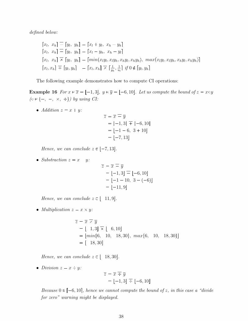
defined below:
rxl, xhs ryl, yhs rxl yl, xh yhs
rxl, xhs ryl, yhs rxl yh, xh yls
rxl, xhs ryl, yhs rminpxlyl, xlyh, xhyl, xhyhq, maxpxlyl, xlyh, xhyl, xhyhqs
rxl, xhs ryl, yhs rxl, xhs r1yh
, 1uls if 0 R ryl, yhs
The following example demonstrates how to compute CI operations:
Example 16 For x P x r1, 3s, y P y r6, 10s. Let us compute the bound of z xy
( P t, , , u) by using CI:
• Addition z x y:
z x y
r1, 3s r6, 10s
r1 6, 3 10s
r7, 13s
Hence, we can conclude z P r7, 13s.
• Substraction z x y:
z x y
r1, 3s r6, 10s
r1 10, 3 p6qs
r11, 9s
Hence, we can conclude z P r11, 9s.
• Multiplication z x y:
z x y
r1, 3s r6, 10s
rmint6,10,18, 30u, maxt6,10,18, 30us
r18, 30s
Hence, we can conclude z P r18, 30s.
• Division z x y:
z x y
r1, 3s r6, 10s
Because 0 P r6, 10s, hence we cannot compute the bound of z, in this case a “divide
for zero” warning might be displayed.
38
For x, x1, ..., xn P R, P t,,,u, and a constant c, we denote:
• x1x2 x1 x2, cx xc x rc, cs,
• c x rc, cs rxs, x c x rc, cs, and
•°n
i1 xi x1 x2 xn.
CI arithmetic assumes that all intervals are independent, even if their corresponding
quantities are dependent. The next example illustrates such a problem.
Example 17 Let x P x r1, 3s. It is easy to see that:
x x r1, 3s r1, 3s
r4, 4s
CI arithmetic assumes the first operand and the second operand to be independent, while
in fact, they represent the same quantity x and the result must be r0, 0s.
This assumption leads to a great loss of precision in a long computation chain, which
is called “error explosion”.
4.2 Affine Interval
Affine interval (AI) was introduced by Stolfi [61, 62] as a model for self-validated numer-
ical analysis. It was proposed to address the “error explosion” problem in conventional
CI. Unlike CI, in AI, the quantities are represented as affine combinations (affine forms)
of certain primitive noise symbols, which stand for sources of uncertainty in the data or
approximations made during the computation.
Definition 23 An Affine interval of x is a formula
:x x0 x1ε1 x2ε2 xnεn
with x P rx0 °n
i |xi|, x0 °n
i |xi|s. x0 is called the central value. For each i P
r1, ns, εi P r1, 1s is a noise symbol, which stands for an independent component of the
total uncertainty. The set of affine interval forms is denoted by :R.
In AI arithmetic, the results of linear operations (i.e., addition, subtraction) are
straightforward operations on AIs. However, the results of nonlinear operations (i.e.,
multiplication, division) are not AI forms. Hence, we need to approximate the nonlinear
parts of the results by introducing new noise symbols.
39
Definition 24 AI arithmetic consists of operations t:, :, :, :u on pairs of AIs as
defined below. Let :x x0°n
i1 xiεi and :y y0°n
i1 yiεi. AI operations are as defined
below::x : :y px0 y0q
°ni1pxi yiqεi
:x : :y px0 y0q °n
i1pxi yiqεi
:x : :y x0y0 °n
i1px0yi xiy0qεi Bεn1
:x : :y :x : p 1:yq, if 0 R rx0
°ni |xi|, x0
°ni |xi|s
where εn1 P r1, 1s is a new noise symbol, B is the maximum value of p°n
i1 xiεiqp°n
i1 yiεiq,
and 1:y
is computed by Chebyshev approximation [61].
Remark 5 An easy approximation of B is p°n
i1 |xi|qp°n
i1 |yi|q
Chebyshev approximation
In general, Chebyshev approximation aims to minimize the maximum absolute error.
Specifically, let F be some space of functions, (polynomials, affine forms, etc.). An element
of F that minimizes the maximum absolute difference from a given function f over some
specified domain Ω is known as a Chebyshev (or minimax) F -approximation to f over Ω.
In particular, for univariate functions, the minimax affine approximation is character-
ized by the following property:
Theorem 1 Let f be a bounded and continuous function from some closed and bounded
interval I ra, bs to R. Let h be the affine function that best approximates f in I under
the minimax error criterion. Then, there exist three distinct points u, v, w P I where the
error fpxq hpxq has maximum magnitude; and the sign of the error alternates when the
three points are considered in ascending order.
This theorem provides an algorithm for finding the optimum approximation in many
cases, via the following corollary:
Theorem 2 Let f be a bounded and twice differentiable function defined on some interval
I ra, bs, whose seconde derivative f2 does not change sign inside I. Let fapxq αx ζ
be its minimax affine approximation in I. Then:
• The coefficient α is simply pfpbq fpaqqpb aq, the slope of the line rpxq that
interpolates the points pa, fpaqq and pb, fpbqq.
• The maximum absolute error will occur twice (with the same sign) at the endpoints
a and b of the range, and once (with the opposite sign) at every interior point u of
I where f 1puq α.
• The independent term ζ is such that αu ζ pfpuq rpuqq2, and the maximum
absolute error is δ |fpuq rpuq|2.
40
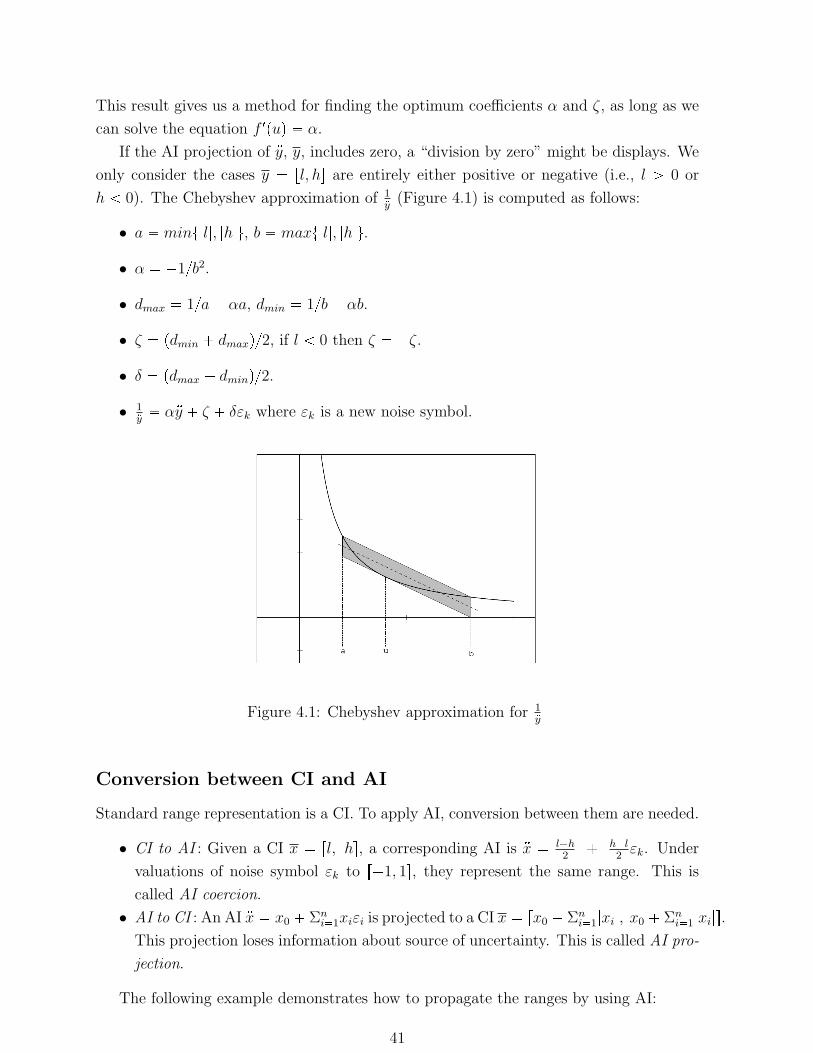
This result gives us a method for finding the optimum coefficients α and ζ, as long as we
can solve the equation f 1puq α.
If the AI projection of :y, y, includes zero, a “division by zero” might be displays. We
only consider the cases y rl, hs are entirely either positive or negative (i.e., l ¡ 0 or
h 0). The Chebyshev approximation of 1:y
(Figure 4.1) is computed as follows:
• a mint|l|, |h|u, b maxt|l|, |h|u.
• α 1b2.
• dmax 1a αa, dmin 1b αb.
• ζ pdmin dmaxq2, if l 0 then ζ ζ.
• δ pdmax dminq2.
• 1:y α:y ζ δεk where εk is a new noise symbol.
Figure 4.1: Chebyshev approximation for 1:y
Conversion between CI and AI
Standard range representation is a CI. To apply AI, conversion between them are needed.
• CI to AI : Given a CI x rl, hs, a corresponding AI is :x lh2 hl
2εk. Under
valuations of noise symbol εk to r1, 1s, they represent the same range. This is
called AI coercion.
• AI to CI : An AI :x x0 Σni1xiεi is projected to a CI x rx0 Σn
i1|xi|, x0 Σni1|xi|s.
This projection loses information about source of uncertainty. This is called AI pro-
jection.
The following example demonstrates how to propagate the ranges by using AI:
41
Example 18 For x P x r1, 3s, y P y r6, 10s. The corresponding AI coercions of
x, y are:
• :x 1 2εx
• :y 2 8εy
Let us compute the bound of z x y ( P t, , , u) by using AI:
• Addition z x y:
:z :x : :y
p1 2εxq : p2 8εyq
3 2εx 8εy
The AI projection of :z is r3 2 8, 3 2 8s r7, 13s. Hence, we can conclude
z P r7, 13s.
• Substraction z x y:
:z :x : :y
p1 2εxq : p2 8εyq
1 2εx 8εy
The AI projection of :z is r128,128s r11, 9s. Hence, we can conclude
that z P r11, 9s.
• Multiplication z x y:
:z :x : :y
p1 2εxq : p2 8εyq
2 4εx 8εy 16ε1
where ε1 is new noise symbol standing for εxεy.
The AI projection of :z is r2 4 8 16, 2 4 8 16s r26, 30s.
Hence, we can conclude that z P r26, 30s.
• Division z x y:
:z :x : :y
p1 2εxq : p2 8εyq
Because 0 P r6, 10s, hence we cannot compute the bound of z, in this case a “divide
for zero” warning might be displayed.
AI is more precise than CI for linear operations, as shown in the next example.
42
Example 19 For x P x r1, 3s, let us consider how to compute the bound of z xx
by using CI and AI.
• CI substraction:
z x x r4, 4s
We hence conclude z P r4, 4s.
• AI substraction: The AI coercion of x is :x 1 2εx. Hence:
:z :x : :x 0
We hence conclude z 0. This result is the correct result of the subtraction pxxq.
However, in AI arithmetic, each time we perform a nonlinear operation, we introduce
a new noise symbol, which is problematic for a program with a large number of nonlinear
operations.
4.3 Extended Affine Interval
AI is more precise than CI for linear operations, but each time we perform a nonlinear
operation, it introduces a new noise symbol. This would be problematic for a program
with a large number of nonlinear operations.
In [27], instead of introducing new noise symbols, coefficients of noise symbols are
replaced with CIs. Arithmetic operations are designed for under approximation, and we
apply similar ideas for over approximation. This is called an extended affine interval
(EAI), which also avoids introduction of new noise symbols for nonlinear operations.
Definition 25 An extended affine interval of x is a formula
px x0 n
k1
xkεk
with x P x0 °n
k1 xkr1, 1s, where εi P r1, 1s is a noise symbol for each i P r1, ns and
xj P R for each j P r0, ns. The set of extended affine intervals is denoted by pR.
The linear operations of EAI arithmetic are designed similarly to those of AI arith-
metic. For nonlinear operations, unlike AI, EAI arithmetic does not need to introduce
new noise symbols. The results of nonlinear operations are guaranteed to be EAIs by ap-
proximating nonlinear parts. For example, let us consider the multiplication of two EAIs.
Let px x0 °n
i1 xiεi, py y0 °n
i1 yiεi. Without loss of generality, assume that
43
°nk1 ykr1, 1s
°nk1 xkr1, 1s. We have: px p py px0
°ni1 xiεiq p py0
°ni1 yiεiq
x0y0 °n
i1px0yi xiy0 xiBqεi, where B °n
i1 yiεi. An easy approximation of B
is°n
k1 ykr1, 1s. Formally, EAI arithmetic is defined as follows:
Definition 26 EAI arithmetic consists of operations
tp, p, p, pu on pairs of EAIs.
Let px x0 °n
i1 xiεi, py y0 °n
i1 yiεi, X °n
k1pxk r1, 1sq, and Y °nk1pyk r1, 1sq. Then,
px p py px0 y0q °n
i1pxi yiqεipx p py px0 y0q °n
i1pxi yiqεipx p py x0y0 °n
i1px0yi xiy0qεi Bpx p py px p p 1pyq if 0 R x0
°nk1 xkr1, 1s
where:
B
$&%p°n
i1 xiY εiq if Y X
p°n
i1 Xyiεiq otherwise
and 1py
is computed by Chebyshev approximation [61].
Similar to AI arithmetic, the commutative property holds for both addition and mul-
tiplication; the associative property only holds for addition; and the distributive property
does not hold.
Remark 6 The over approximation B may conceal some noise symbols. If we are sensi-
tive to this matter, B can be modified as:
B αp°n
i1 xiY εiq βp°n
i1 Xyiεiq
with α |X|
p|X| |Y |qand β p1 αq.
Conversion between CI and EAI
Standard range representation is a CI. To apply EAI, the conversion between them are
needed.
• CI to EAI : Given a CI x rl, hs, a corresponding EAI is x lh2 hl
2εk. Under
valuations of a noise symbol εk to r1, 1s, they represent the same range. This is
called EAI coercion.
• EAI to CI : An EAI x x0 Σni1xiεi is projected to a CI x x0 Σn
i1xir1, 1s.
Replacement of a noise symbol εk to r1, 1s loses information about source of un-
certainty. This is called EAI projection.
44
The following example demonstrates how to propagate the ranges using EAI:
Example 20 For x P x r1, 3s, y P y r6, 10s. The corresponding EAI coercions of
x, y are:
• x 1 2εx
• y 2 8εy
Let us compute the bound of z x y ( P t, , , u) by using EAI:
• Addition z x y:
z x y
p1 2εxq p2 8εyq
3 2εx 8εy
The EAI projection of z is 3 2r1, 1s 8r1, 1s r7, 13s.
Hence, we can conclude that z P r7, 13s.
• Substraction z x y:
z x y
p1 2εxq p2 8εyq
1 2εx 8εy
The AI projection of :z is 1 2r1, 1s 8r1, 1s r11, 9s.
Hence, we can conclude that z P r11, 9s.
• Multiplication z x y:
z x y
p1 2εxq p2 8εyq
2 4εx 8εy B
where X 2r1, 1s r2, 2s and Y 8r1, 1s r8, 8s.
Because X Y . Hence, B 8εyX r16, 16sεy. Then, z 2 4εx r8, 24sεy
The AI projection of :z is 2 4r1, 1s r8, 24sr1, 1s r26, 30s.
Hence, we can conclude that z P r26, 30s
• Division z x y:
z x y
p1 2εxq p2 8εyq
45
Because 0 P r6, 10s, hence we cannot compute the bound of z, in this case a “divide
for zero” warning might be displayed.
Although EAI does not introduce new noise symbols, this does not mean EAI arith-
metic is always less precise than AI arithmetic. AI arithmetic only advances in cases when
we reuse the results of some nonlinear parts. Let us consider the example below:
Example 21 Let z x x; t z z and x P r1, 31s.
The bound of t is computed based on AI and EAI arithmetics as follows:
• AI arithmetic: :x 12εx, :z 14εx4ε1 where ε1 is introduced for multiplication
εxεx.
:t :z ::z 0
• EAI arithmetic: px 12εx, pz 1r0, 8sεx.
t zz r8, 8sεx
The bound of :z, [0,0], lies within the bound of pz, [-8,8]. So, AI arithmetic is more precise
in this case. However, if we compute the bound of t x x x x without reusing the
multiplication x x, then both AI arithmetic and EAI arithmetic return the same bound.
:t, pt can be computed in a similar way. To keep things simple, we omit the details of these
computations here.
4.4 Positive-noise Affine Interval
In this section, we propose another way to “extend” AI which tries to reduce the over
approximation in the nonlinear operations.
We start by an example:
Example 22 Let us consider the multiplication: x εk εk.
It easily sees that x P r0, 1s for all εk P r1, 1s. However, by applying AI multiplication
and EAI multiplication, we get:
• AI multiplication :x εk :εk. We have:
:x εn1, where B 1 and εn1 is new noise symbol.
Hence, :x P r1, 1s (instead of r0, 1s) and we already lose information about εk.
• EAI multiplication x εkεk. We have:
x r1, 1sεk.
Hence, x P r1, 1s (instead of r0, 1s).
46
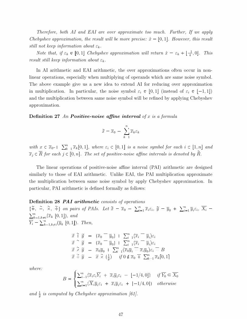
Therefore, both AI and EAI are over approximate too much. Further, If we apply
Chebyshev approximation, the result will be more precise: x r0, 1s. However, this result
still not keep information about εk.
Note that, if εk P r0, 1s Chebyshev approximation will return x εk r14
, 0s. This
result still keep information about εk.
In AI arithmetic and EAI arithmetic, the over approximations often occur in non-
linear operations, especially when multiplying of operands which are same noise symbol.
The above example give us a new idea to extend AI for reducing over approximation
in multiplication. In particular, the noise symbol εi P r0, 1s (instead of εi P r1, 1s)
and the multiplication between same noise symbol will be refined by applying Chebyshev
approximation.
Definition 27 An Positive-noise affine interval of x is a formula
rx x0 n
k1
xkεk
with x P x0 °n
k1 xkr0, 1s, where εi P r0, 1s is a noise symbol for each i P r1, ns and
xj P R for each j P r0, ns. The set of positive-noise affine intervals is denoted by rR.
The linear operations of positive-noise affine interval (PAI) arithmetic are designed
similarly to those of EAI arithmetic. Unlike EAI, the PAI multiplication approximate
the multiplication between same noise symbol by apply Chebyshev approximation. In
particular, PAI arithmetic is defined formally as follows:
Definition 28 PAI arithmetic consists of operations
tr, r, r, ru on pairs of PAIs. Let rx x0 °n
i1 xiεi, ry y0 °n
i1 yiεi, Xi °nk1,kipxk r0, 1sq, and
Yi °n
k1,kipyk r0, 1sq. Then,
rx r ry px0 y0q °n
i1pxi yiqεirx r ry px0 y0q °n
i1pxi yiqεirx r ry x0y0 °n
i1px0yi xiy0qεi Brx r ry rx r p 1ryq if 0 R x0
°nk1 xkr0, 1s
where:
B
$&%°n
i1pxiεiYi xiyiεi r14, 0sq if Y0 X0°ni1pX iyiεi xiyiεi r14, 0sq otherwise
and 1ry
is computed by Chebyshev approximation [61].
47
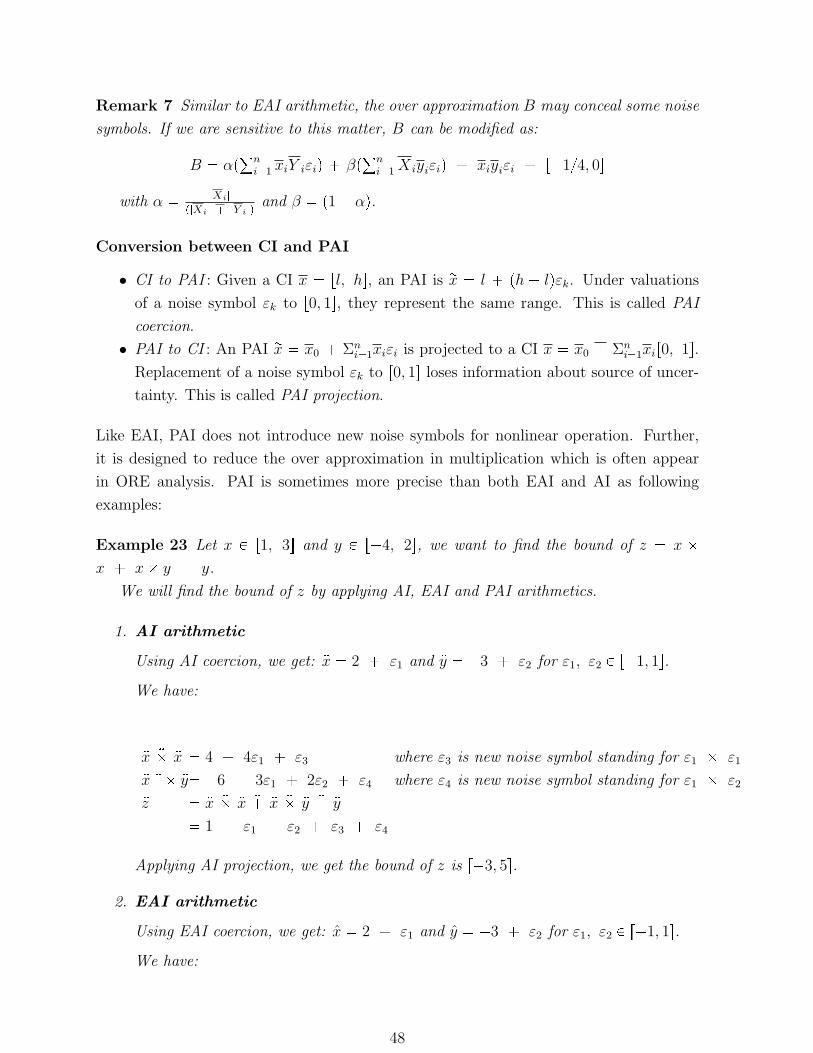
Remark 7 Similar to EAI arithmetic, the over approximation B may conceal some noise
symbols. If we are sensitive to this matter, B can be modified as:
B αp°n
i1 xiY iεiq βp°n
i1 X iyiεiq xiyiεi r14, 0s
with α |Xi|
p|Xi| |Y i|qand β p1 αq.
Conversion between CI and PAI
• CI to PAI : Given a CI x rl, hs, an PAI is rx l ph lqεk. Under valuations
of a noise symbol εk to r0, 1s, they represent the same range. This is called PAI
coercion.
• PAI to CI : An PAI rx x0 Σni1xiεi is projected to a CI x x0 Σn
i1xir0, 1s.
Replacement of a noise symbol εk to r0, 1s loses information about source of uncer-
tainty. This is called PAI projection.
Like EAI, PAI does not introduce new noise symbols for nonlinear operation. Further,
it is designed to reduce the over approximation in multiplication which is often appear
in ORE analysis. PAI is sometimes more precise than both EAI and AI as following
examples:
Example 23 Let x P r1, 3s and y P r4, 2s, we want to find the bound of z x
x x y y.
We will find the bound of z by applying AI, EAI and PAI arithmetics.
1. AI arithmetic
Using AI coercion, we get: :x 2 ε1 and :y 3 ε2 for ε1, ε2 P r1, 1s.
We have:
:x : :x 4 4ε1 ε3 where ε3 is new noise symbol standing for ε1 ε1
:x : :y 6 3ε1 2ε2 ε4 where ε4 is new noise symbol standing for ε1 ε2
:z :x : :x : :x : :y : :y
1 ε1 ε2 ε3 ε4
Applying AI projection, we get the bound of z is r3, 5s.
2. EAI arithmetic
Using EAI coercion, we get: x 2 ε1 and y 3 ε2 for ε1, ε2 P r1, 1s.
We have:
48
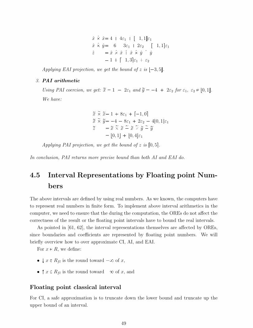
x x 4 4ε1 r1, 1sε1
x y 6 3ε1 2ε2 r1, 1sε1
z x x x y y
1 r1, 3sε1 ε2
Applying EAI projection, we get the bound of z is r3, 5s.
3. PAI arithmetic
Using PAI coercion, we get: rx 1 2ε1 and ry 4 2ε2 for ε1, ε2 P r0, 1s.
We have:
rx r rx 1 8ε1 r1, 0srx r ry 4 8ε1 2ε2 4r0, 1sε1rz rx r rx r rx r ry r ry r0, 1s r0, 4sε1
Applying PAI projection, we get the bound of z is r0, 5s.
In conclusion, PAI returns more precise bound than both AI and EAI do.
4.5 Interval Representations by Floating point Num-
bers
The above intervals are defined by using real numbers. As we known, the computers have
to represent real numbers in finite form. To implement above interval arithmetics in the
computer, we need to ensure that the during the computation, the OREs do not affect the
correctness of the result or the floating point intervals have to bound the real intervals.
As pointed in [61, 62], the interval representations themselves are affected by OREs,
since boundaries and coefficients are represented by floating point numbers. We will
briefly overview how to over approximate CI, AI, and EAI.
For x P R, we define:
• Ó x P Rfl is the round toward 8 of x,
• Ò x P Rfl is the round toward 8 of x, and
Floating point classical interval
For CI, a safe approximation is to truncate down the lower bound and truncate up the
upper bound of an interval.
49
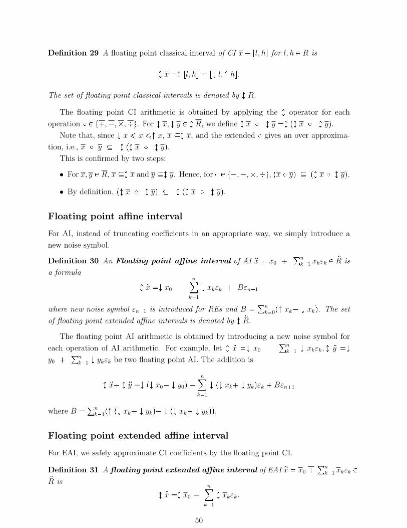
Definition 29 A floating point classical interval of CI x rl, hs for l, h P R is
Ù x Ù rl, hs rÓ l, Ò hs.
The set of floating point classical intervals is denoted by Ù R.
The floating point CI arithmetic is obtained by applying the Ù operator for each
operation P t,,,u. For Ù x, Ù y P Ù R, we define Ù x Ù y Ù pÙ x Ù yq.
Note that, since Ó x ¤ x ¤Ò x, x Ù x, and the extended gives an over approxima-
tion, i.e., x y Ù pÙ x Ù yq.
This is confirmed by two steps:
• For x, y P R, x Ù x and y Ù y. Hence, for P t,,,u, px yq pÙ x Ù yq.
• By definition, pÙ x Ù yq Ù pÙ x Ù yq.
Floating point affine interval
For AI, instead of truncating coefficients in an appropriate way, we simply introduce a
new noise symbol.
Definition 30 An Floating point affine interval of AI :x x0 °n
k1 xkεk P :R is
a formula
Ù :x Ó x0 n
k1
Ó xkεk Bεn1
where new noise symbol εn1 is introduced for REs and B °n
k0pÒ xk Ó xkq. The set
of floating point extended affine intervals is denoted by Ù :R.
The floating point AI arithmetic is obtained by introducing a new noise symbol for
each operation of AI arithmetic. For example, let Ù :x Ó x0 °n
k1 Ó xkεk, Ù :y Ó
y0 °n
k1 Ó ykεk be two floating point AI. The addition is
Ù :x Ù :y Ó pÓ x0 Ó y0q n
k1
Ó pÓ xk Ó ykqεk Bεn1
where B °n
k1pÒ pÓ xk Ó ykq Ó pÓ xk Ó ykqq.
Floating point extended affine interval
For EAI, we safely approximate CI coefficients by the floating point CI.
Definition 31 A floating point extended affine interval of EAI px x0 °n
k1 xkεk PpR is
Ù px Ù x0 n
k1
Ù xkεk.
50
The set of floating point extended affine intervals is denoted by Ù pR.
The floating point EAI arithmetic is obtained by replacing each CI at a coefficient by
the floating point CI.
From now on, we will apply floating point CI, floating point AI, and floating point
EAI, instead of CI, AI, and EAI, respectively.
51
Chapter 5
Abstraction for ORE Problem
The abstract value of a variable aims to cover all of its possible values at one program
location. For the ORE problem, the abstract value is a pair of fixed point and roundoff
error ranges. In this chapter, we will show three kinds of abstractions based on CI, AI,
and EAI range representations.
5.1 CI Abstraction for ORE Problem
For estimation of propagations of REs based on CI, we apply CI arithmetic (Definition 22)
to Float64-to-fixed16 ORE arithmetic (Definition 11).
Definition 32 The set Φ of CI abstract numbers is:
Φ tpfxp, rdfq|fxp, rdf P Ru
CI abstract arithmetic consists of t`, a, b, cu on pairs of CI abstract numbers.
Let pxf , xrq, pyf , yrq P Φ be CI abstract numbers. The CI abstract operators are defined
below:
pxf , xrq ` pyf , yrqpxf yf , xr yr rδ, δsq
pxf , xrq a pyf , yrqpxf yf , xr yr rδ, δsq
pxf , xrq b pyf , yrqpxf yf , xr yf xf yr xr yr rδ, δsq
pxf , xrq c pyf , yrqpxf yf , pxf xrq pyf yrq xf yf rδ, δsq
where δ, δ, δ, δ is given in Equation 2.2.
To illustrate how to create CI abstract numbers and compute CI abstract arithmetic,
we consider the following example:
52
Example 24 The CI abstract numbers pxf , xrq, pyf , yrq for variables x, y, respectively,
in Example 3 are #xf r1, 3s
xr r25, 25s#yf r10, 10s
yr r25, 25s
since fp 5, the REs of x and y are in r2fp1, 2fp1s r25, 25s p r0.03125, 0.03125sq.
Then, at the line 2 (rst x x), prstf , rstrq pxf , xrq b pxf , xrq is projected as
follows:rstf xf xf
pr1, 3s r1, 3s
r3, 9s
rstr 2 xf xr xr xr δ
r0.219726563, 0.219726563s
CI abstract comparison operators
Instead of nondeterministic transitions at a conditional branch, the conditional expres-
sion can often be evaluated by using abstract environment. This is useful in avoiding
unnecessary execution paths. The abstract comparison operators are defined by using
Float-to-Fixed comparison operators as follows:
Replacing pxf , xrq, pyf , yrq in Float-to-fixed ORE comparison operators (Definition 8)
with CI abstract numbers pxf , xrq, pyf , yrq we obtain CI abstract comparison operators:
Definition 33 Let pxf , xrq, pyf , yrq P Φ, let x pxf xrq, and let y pyf yrq.
ppxf , xrq pyf , yrqq
$'''&'''%true if @u P x @v P y.u v ^ @u P xf @v P yf .u v
false if @u P x @v P y.u ¥ v ^ @u P xf @v P yf .u ¥ v
unknown otherwise
ppxf , xrqpyf , yrqq
$'''&'''%true if p@u P xf @v P yf .u v ^ @u P xr @v P yr.u vq
false if pxf , xrq pyf , yrq _ pyf , yrq pxf , xrq
unknown otherwise
The following example illustrates how to evaluate CI abstract comparison operator .
Example 25 Use pxf , xrq, and pyf , yrq as in Example 24. pxf , xrq r0, 0s is evaluated
as follows:
53
xxf xr
r1, 3s r25, 25s
r1 25, 3 25s
Since 0 P r1 25, 3 25s, we can conclude that pxf , xrq 0 is unknown.
5.2 AI Abstract Numbers
For estimation of propagations of REs based on AI, we apply AI arithmetic (Definition 24)
to Float64-to-Fixed16 ORE arithmetic (Definition 11).
Definition 34 The set :Φ of AI abstract numbers is:
:Φ tpfxp, rdfq|fxp, rdf P :Ru
AI abstract arithmetic consists of t : , :a, :b, :cu on pairs of AI abstract numbers.
Let AI abstract numbers p:xf , :xrq, p:yf , :yrq P :Φ. The AI abstract operators are defined
below:
p:xf , :xrq : p:yf , :yrqp:xf : :yf , :xr : :yr : δεpq
p:xf , :xrq :a p:yf , :yrqp:xf : :yf , :xr : :yr : δεpq
p:xf , :xrq :b p:yf , :yrq p:xf ::yf , :xr ::yf : :xf ::yr : :xr ::yr : δεpq
p:xf , :xrq :c p:yf , :yrqp:xf : :yf , p:xf : :xrq : p:yf : :yrq : :xf : :yf : δεpq
whereδ, δ, δ, δ are given in Equation 2.2 and εp is a new noise symbol.
To illustrate how to create AI abstract numbers and compute AI abstract arithmetic,
we consider following example:
Example 26 The AI abstract numbers p:xf , :xrq, p:yf , :yrq for variables x, y, respectively,
in Example 3 are #:xf 1 2ε1
:xr 25ε3#:yf 10ε2
:yr 25ε4
since fp 5, the REs of x and y are in r2fp1, 2fp1s r25, 25s p r0.03125, 0.03125sq.
Then, at the line 2 (rst x x), p :rstf , :rstrq p:xf , :xrq :b p:xf , :xrq is projected as
54
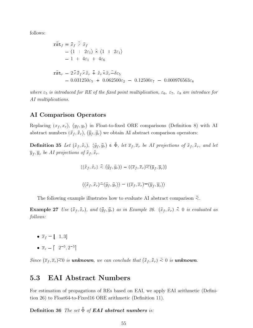
follows:
:rstf :xf : :xf
p1 2ε1q : p1 2ε1q
1 4ε1 4ε6
:rstr 2::xf ::xr : :xr ::xr :δε5
0.031250ε5 0.062500ε2 0.12500ε7 0.000976563ε8
where ε5 is introduced for RE of the fixed point multiplication, ε6, ε7, ε8 are introduce for
AI multiplications.
AI Comparison Operators
Replacing pxf , xrq, pyf , yrq in Float-to-fixed ORE comparisons (Definition 8) with AI
abstract numbers p:xf , :xrq, p:yf , :yrq we obtain AI abstract comparison operators:
Definition 35 Let p:xf , :xrq, p:yf , :yrq P :Φ, let xf , xr be AI projections of :xf , :xr, and let
yf , yr be AI projections of :xf , :xr.
pp:xf , :xrq : p:yf , :yrqq ppxf , xrq pyf , yrqq
pp:xf , :xrq:p:yf , :yrqq ppxf , xrqpyf , yrqq
The following example illustrates how to evaluate AI abstract comparison : .
Example 27 Use p:xf , :xrq, and p:yf , :yrq as in Example 26. p:xf , :xrq : 0 is evaluated as
follows:
• xf r1, 3s
• xr r25, 25s
Since pxf , xrq 0 is unknown, we can conclude that p:xf , :xrq : 0 is unknown.
5.3 EAI Abstract Numbers
For estimation of propagations of REs based on EAI, we apply EAI arithmetic (Defini-
tion 26) to Float64-to-Fixed16 ORE arithmetic (Definition 11).
Definition 36 The set pΦ of EAI abstract numbers is:
55
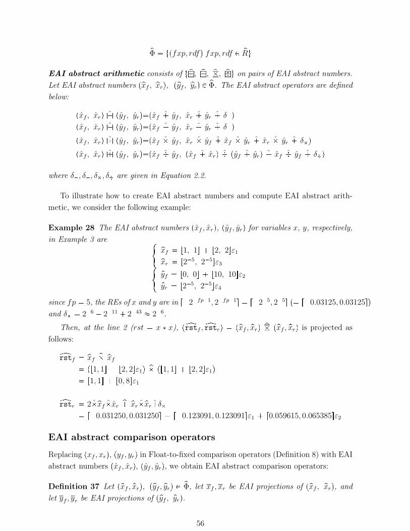
pΦ tpfxp, rdfq|fxp, rdf P pRuEAI abstract arithmetic consists of t p , pa, pb, pcu on pairs of EAI abstract numbers.
Let EAI abstract numbers ppxf , pxrq, ppyf , pyrq P pΦ. The EAI abstract operators are defined
below:
pxf , xrq ˆ pyf , yrqpxf yf , xr yr δq
pxf , xrq a pyf , yrqpxf yf , xr yr δq
pxf , xrq b pyf , yrqpxf yf , xr yf xf yr xr yr δq
pxf , xrq c pyf , yrqpxf yf , pxf xrq pyf yrq xf yf δq
where δ, δ, δ, δ are given in Equation 2.2.
To illustrate how to create EAI abstract numbers and compute EAI abstract arith-
metic, we consider the following example:
Example 28 The EAI abstract numbers pxf , xrq, pyf , yrq for variables x, y, respectively,
in Example 3 are # pxf r1, 1s r2, 2sε1pxr r25, 25sε3# pyf r0, 0s r10, 10sε2pyr r25, 25sε4
since fp 5, the REs of x and y are in r2fp1, 2fp1s r25, 25s p r0.03125, 0.03125sq
and δ 26 211 243 26.
Then, at the line 2 (rst x x), pyrstf ,yrstrq ppxf , pxrq pb ppxf , pxrq is projected as
follows:
yrstf pxf p pxf
pr1, 1s r2, 2sε1q p pr1, 1s r2, 2sε1q
r1, 1s r0, 8sε1
yrstr 2pxf xr p pxrpxrδ
r0.031250, 0.031250s r0.123091, 0.123091sε1 r0.059615, 0.065385sε2
EAI abstract comparison operators
Replacing pxf , xrq, pyf , yrq in Float-to-fixed comparison operators (Definition 8) with EAI
abstract numbers pxf , xrq, pyf , yrq, we obtain EAI abstract comparison operators:
Definition 37 Let ppxf , pxrq, ppyf , pyrq P pΦ, let xf , xr be EAI projections of ppxf , pxrq, and
let yf , yr be EAI projections of ppyf , pyrq.
56
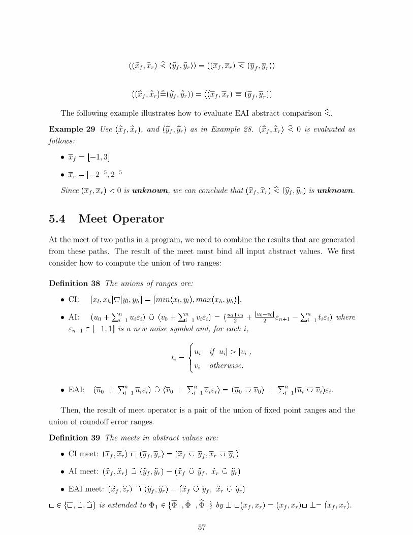
pppxf , pxrq p ppyf , pyrqq ppxf , xrq pyf , yrqq
pppxf , pxrqpppyf , pyrqq ppxf , xrq pyf , yrqq
The following example illustrates how to evaluate EAI abstract comparison p .
Example 29 Use ppxf , pxrq, and ppyf , pyrq as in Example 28. ppxf , pxrq p 0 is evaluated as
follows:
• xf r1, 3s
• xr r25, 25
Since pxf , xrq 0 is unknown, we can conclude that ppxf , pxrq p ppyf , pyrq is unknown.
5.4 Meet Operator
At the meet of two paths in a program, we need to combine the results that are generated
from these paths. The result of the meet must bind all input abstract values. We first
consider how to compute the union of two ranges:
Definition 38 The unions of ranges are:
• CI: rxl, xhsYryl, yhs rminpxl, ylq, maxpxh, yhqs.
• AI: pu0 °n
i1 uiεiq :Y pv0 °n
i1 viεiq pu0v0
2 |u0v0|
2εn1
°ni1 tiεiq where
εn1 P r1, 1s is a new noise symbol and, for each i,
ti
$&%ui if |ui| ¡ |vi|,
vi otherwise.
• EAI: pu0 °n
i1 uiεiq pY pv0 °n
i1 viεiq pu0 Y v0q °n
i1pui Y viqεi.
Then, the result of meet operator is a pair of the union of fixed point ranges and the
union of roundoff error ranges.
Definition 39 The meets in abstract values are:
• CI meet: pxf , xrq \ pyf , yrq pxf Y yf , xr Y yrq
• AI meet: p:xf , :xrq :\ p:yf , :yrq p:xf :Y :yf , :xr :Y :yrq
• EAI meet: ppxf , pzrq p\ ppyf , pyrq ppxf pY pyf , pxr pY pyrq
\ P t\, :\, p\u is extended to ΦK P tΦK, :ΦK, pΦKu by K \pxf , xrq pxf , xrq\ K pxf , xrq.
57
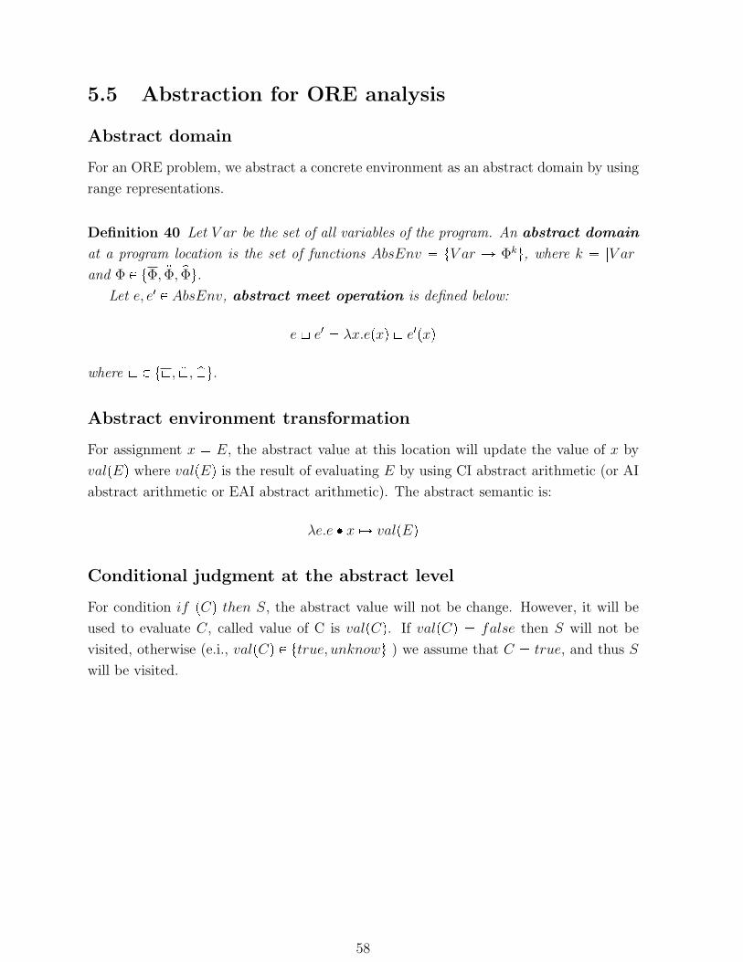
5.5 Abstraction for ORE analysis
Abstract domain
For an ORE problem, we abstract a concrete environment as an abstract domain by using
range representations.
Definition 40 Let V ar be the set of all variables of the program. An abstract domain
at a program location is the set of functions AbsEnv tV ar Ñ Φku, where k |V ar|
and Φ P tΦ, :Φ, pΦu.Let e, e1 P AbsEnv, abstract meet operation is defined below:
e\ e1 λx.epxq \ e1pxq
where \ P t\, :\, p\u.Abstract environment transformation
For assignment x E, the abstract value at this location will update the value of x by
valpEq where valpEq is the result of evaluating E by using CI abstract arithmetic (or AI
abstract arithmetic or EAI abstract arithmetic). The abstract semantic is:
λe.e x ÞÑ valpEq
Conditional judgment at the abstract level
For condition if pCq then S, the abstract value will not be change. However, it will be
used to evaluate C, called value of C is valpCq. If valpCq false then S will not be
visited, otherwise (e.i., valpCq P ttrue, unknowu ) we assume that C true, and thus S
will be visited.
58
Chapter 6
ORE Analysis as Weighted Model
Checking Problem
As can be seen in Chapter 3, dataflow analysis can be treated as weighted model checking
and abstraction. In this chapter, we will exploit how this idea of dataflow analysis can
be applied to solve the ORE problems. In particular, using weighted model checking as a
back-end framework, we first design: a weighted transition system for the ORE problem
in Section 6.1 and 6.2. After that, in Section 6.3, we show how the ORE analysis can
be reduced to the weighted model checking problem over the resulting weighted tran-
sition system. Finally, we implement our ORE analysis framework in a prototype tool
called CANA. Details of the implementation and some experimental results are given in
Section 6.4.
6.1 Weighted Domain for the ORE Problem
Weight Design
The standard definition of a weight domain has the base set of weights D AbsEnv Ñ
AbsEnv. We then define the weight domain for D as follows:
Definition 41 The weight domain (bounded idempotent semiring) S pD,`,b,0,1q
with
59
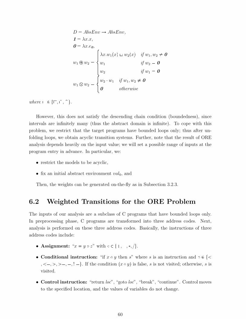
D AbsEnv Ñ AbsEnv,
1 λx.x,
0 λx.e0,
w1 ` w2
$'''&'''%λx.w1pxq \ w2pxq if w1, w2 0
w1 if w2 0
w2 if w1 0
w1 b w2
$&%w2 w1 if w1, w2 0
0 otherwise
where \ P t\, :\, p\u.However, this does not satisfy the descending chain condition (boundedness), since
intervals are infinitely many (thus the abstract domain is infinite). To cope with this
problem, we restrict that the target programs have bounded loops only; thus after un-
folding loops, we obtain acyclic transition systems. Further, note that the result of ORE
analysis depends heavily on the input value; we will set a possible range of inputs at the
program entry in advance. In particular, we:
• restrict the models to be acyclic,
• fix an initial abstract environment val0, and
Then, the weights can be generated on-the-fly as in Subsection 3.2.3.
6.2 Weighted Transitions for the ORE Problem
The inputs of our analysis are a subclass of C programs that have bounded loops only.
In preprocessing phase, C programs are transformed into three address codes. Next,
analysis is performed on these three address codes. Basically, the instructions of three
address codes include:
• Assignment: “x y z” with P t,, , u.
• Conditional instruction: “if x y then s” where s is an instruction and P t
, ,¡,¡,, ! u. If the condition px yq is false, s is not visited; otherwise, s is
visited.
• Control instruction: “return loc”, “goto loc”, “break”, “continue”. Control moves
to the specified location, and the values of variables do not change.
60
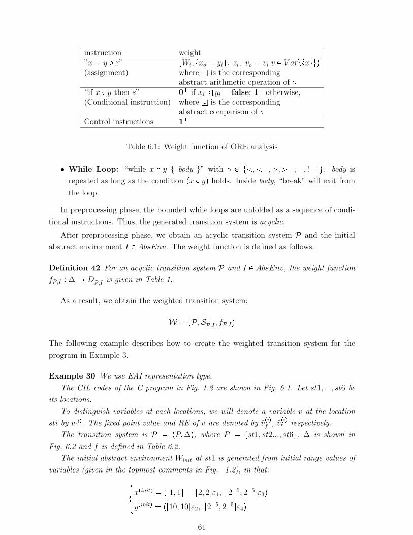
instruction weight”x y z” pWi, txo yi e zi, vo vi|v P V arztxuuq(assignment) where e is the corresponding
abstract arithmetic operation of “if x y then s” 0 if xi e yi false; 1 otherwise,(Conditional instruction) where e is the corresponding
abstract comparison of Control instructions 1
Table 6.1: Weight function of ORE analysis
• While Loop: “while x y body ” with P t , ,¡,¡,, ! u. body is
repeated as long as the condition px yq holds. Inside body, “break” will exit from
the loop.
In preprocessing phase, the bounded while loops are unfolded as a sequence of condi-
tional instructions. Thus, the generated transition system is acyclic.
After preprocessing phase, we obtain an acyclic transition system P and the initial
abstract environment I P AbsEnv. The weight function is defined as follows:
Definition 42 For an acyclic transition system P and I P AbsEnv, the weight function
fP,I : ∆ Ñ DP,I is given in Table 1.
As a result, we obtain the weighted transition system:
W pP ,SP,I , fP,Iq
The following example describes how to create the weighted transition system for the
program in Example 3.
Example 30 We use EAI representation type.
The CIL codes of the C program in Fig. 1.2 are shown in Fig. 6.1. Let st1, ..., st6 be
its locations.
To distinguish variables at each locations, we will denote a variable v at the location
sti by vpiq. The fixed point value and RE of v are denoted by vpiqf , v
piqr respectively.
The transition system is P pP, ∆q, where P tst1, st2..., st6u, ∆ is shown in
Fig. 6.2 and f is defined in Table 6.2.
The initial abstract environment Winit at st1 is generated from initial range values of
variables (given in the topmost comments in Fig. 1.2), in that:$&%xpinitq pr1, 1s r2, 2sε1, r25, 25sε3q
ypinitq pr10, 10sε2, r25, 25sε4q
61
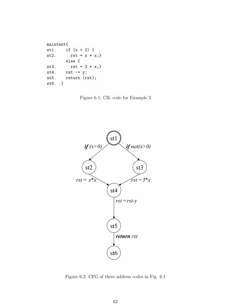
maintest
st1. if (x > 0)
st2. rst = x * x;
else
st3. rst = 3 * x;
st4. rst -= y;
st5. return (rst);
st6.
Figure 6.1: CIL code for Example 3
st1
st2 st3
st4
if
(x>0) if not(x>0)
rst
= x*x rst
=3*x
rst
=rst-y
st6
st5return
rst
Figure 6.2: CFG of three address codes in Fig. 6.1
62
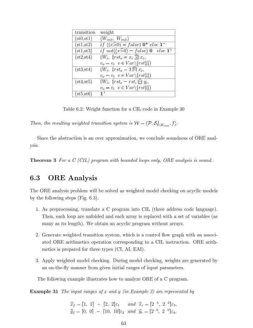
transition weight(st0,st1) pWinit, Winitq(st1,st2) if ppxp¡0q falseq 0 else 1
(st1,st3) if notppxp¡0q falseq 0 else 1
(st2,st4) pWi, trsto xi pb xi,vo vi| v P V arztrstuuq
(st3,st4) pWi, trsto 3 pb xi,vo vi| v P V arztrstuuq
(st4,st5) pWi, trsto rsti pa yi,vo vi| v P V arztrstuuq
(st5,st6) 1
Table 6.2: Weight function for a CIL code in Example 30
Then, the resulting weighted transition system is W pP ,SP,Winit
, fq.
Since the abstraction is an over approximation, we conclude soundness of ORE anal-
ysis.
Theorem 3 For a C (CIL) program with bounded loops only, ORE analysis is sound.
6.3 ORE Analysis
The ORE analysis problem will be solved as weighted model checking on acyclic models
by the following steps (Fig. 6.3).
1. As preprocessing, translate a C program into CIL (three address code language).
Then, each loop are unfolded and each array is replaced with a set of variables (as
many as its length). We obtain an acyclic program without arrays.
2. Generate weighted transition system, which is a control flow graph with an associ-
ated ORE arithmetics operation corresponding to a CIL instruction. ORE arith-
metics is prepared for three types (CI, AI, EAI).
3. Apply weighted model checking. During model checking, weights are generated by
an on-the-fly manner from given initial ranges of input parameters.
The following example illustrates how to analyze ORE of a C program.
Example 31 The input ranges of x and y (in Example 3) are represented by
pxf r1, 1s r2, 2sε1 and pxr r25, 25sε3,pyf r0, 0s r10, 10sε2 and pyr r25, 25sε4.
63
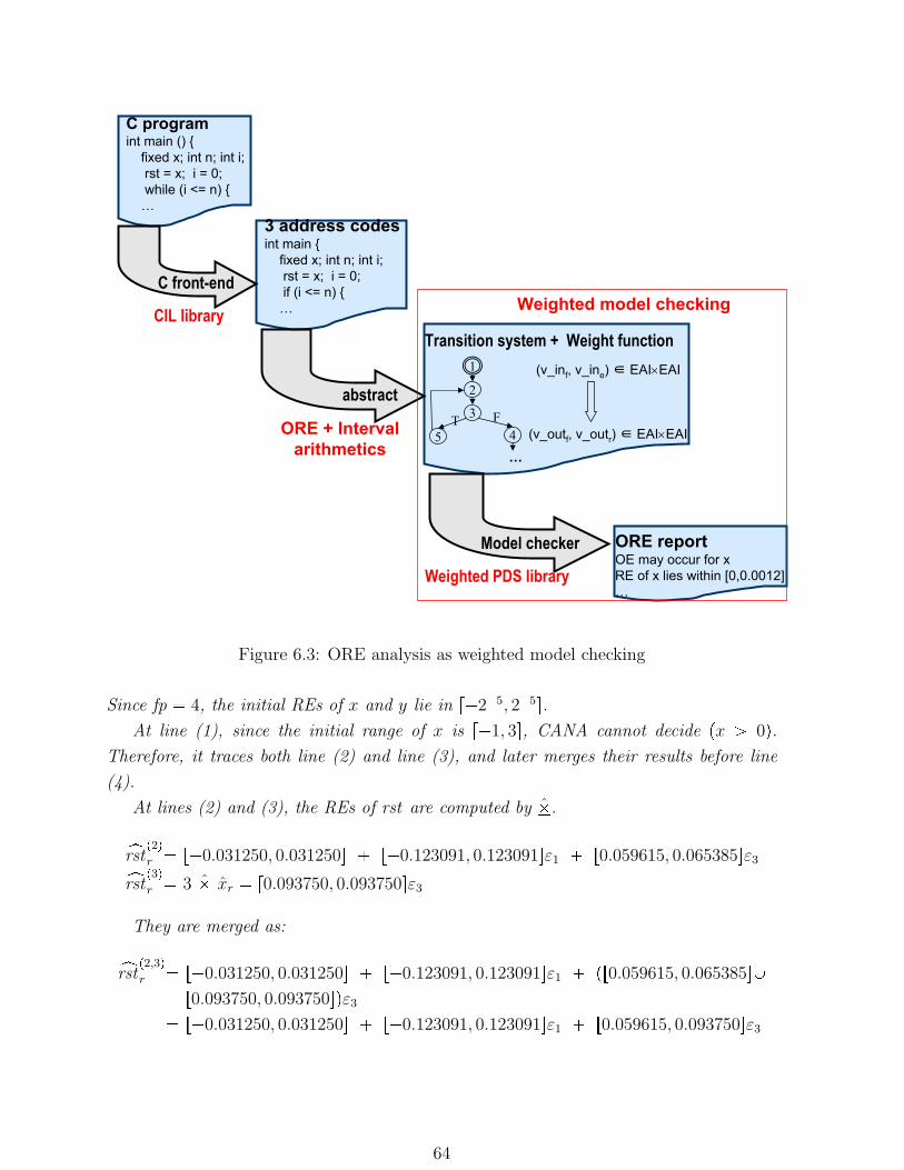
C program int
main () fixed x; int
n; int
i;rst
= x; i = 0; while (i <= n)
…
ORE reportOE may occur for xRE of x lies within [0,0.0012]…
(v_inf
, v_ine
) ∈ EAI×EAI
(v_outf
, v_outr
) ∈ EAI×EAI
1
2
3
5 4T F
…
Transition system + Weight function
3 address codesint
main fixed x; int
n; int
i;rst
= x; i = 0; if (i <= n)
…
C front-end
abstract
Model checker
ORE + Intervalarithmetics
Weighted PDS library
CIL library Weighted model checking
Figure 6.3: ORE analysis as weighted model checking
Since fp 4, the initial REs of x and y lie in r25, 25s.
At line (1), since the initial range of x is r1, 3s, CANA cannot decide px ¡ 0q.
Therefore, it traces both line (2) and line (3), and later merges their results before line
(4).
At lines (2) and (3), the REs of rst are computed by b.
xrst p2qr r0.031250, 0.031250s r0.123091, 0.123091sε1 r0.059615, 0.065385sε3xrst p3qr 3 xr r0.093750, 0.093750sε3
They are merged as:
xrst p2,3q
r r0.031250, 0.031250s r0.123091, 0.123091sε1 pr0.059615, 0.065385sY
r0.093750, 0.093750sqε3
r0.031250, 0.031250s r0.123091, 0.123091sε1 r0.059615, 0.093750sε3
64
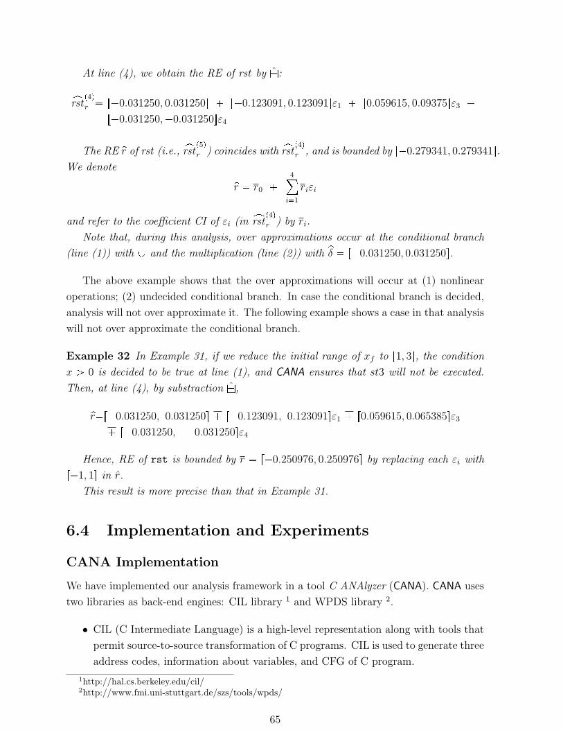
At line (4), we obtain the RE of rst by a:
xrst p4qr r0.031250, 0.031250s r0.123091, 0.123091sε1 r0.059615, 0.09375sε3
r0.031250,0.031250sε4
The RE pr of rst (i.e., xrst p5qr ) coincides with xrst p4qr , and is bounded by r0.279341, 0.279341s.
We denote pr r0 4
i1
riεi
and refer to the coefficient CI of εi (in xrst p4qr ) by ri.
Note that, during this analysis, over approximations occur at the conditional branch
(line (1)) with Y and the multiplication (line (2)) with pδ r0.031250, 0.031250s.
The above example shows that the over approximations will occur at (1) nonlinear
operations; (2) undecided conditional branch. In case the conditional branch is decided,
analysis will not over approximate it. The following example shows a case in that analysis
will not over approximate the conditional branch.
Example 32 In Example 31, if we reduce the initial range of xf to r1, 3s, the condition
x ¡ 0 is decided to be true at line (1), and CANA ensures that st3 will not be executed.
Then, at line (4), by substraction a,
prr0.031250, 0.031250s r0.123091, 0.123091sε1 r0.059615, 0.065385sε3
r0.031250, 0.031250sε4
Hence, RE of rst is bounded by r r0.250976, 0.250976s by replacing each εi with
r1, 1s in r.
This result is more precise than that in Example 31.
6.4 Implementation and Experiments
CANA Implementation
We have implemented our analysis framework in a tool C ANAlyzer (CANA). CANA uses
two libraries as back-end engines: CIL library 1 and WPDS library 2.
• CIL (C Intermediate Language) is a high-level representation along with tools that
permit source-to-source transformation of C programs. CIL is used to generate three
address codes, information about variables, and CFG of C program.
1http://hal.cs.berkeley.edu/cil/2http://www.fmi.uni-stuttgart.de/szs/tools/wpds/
65
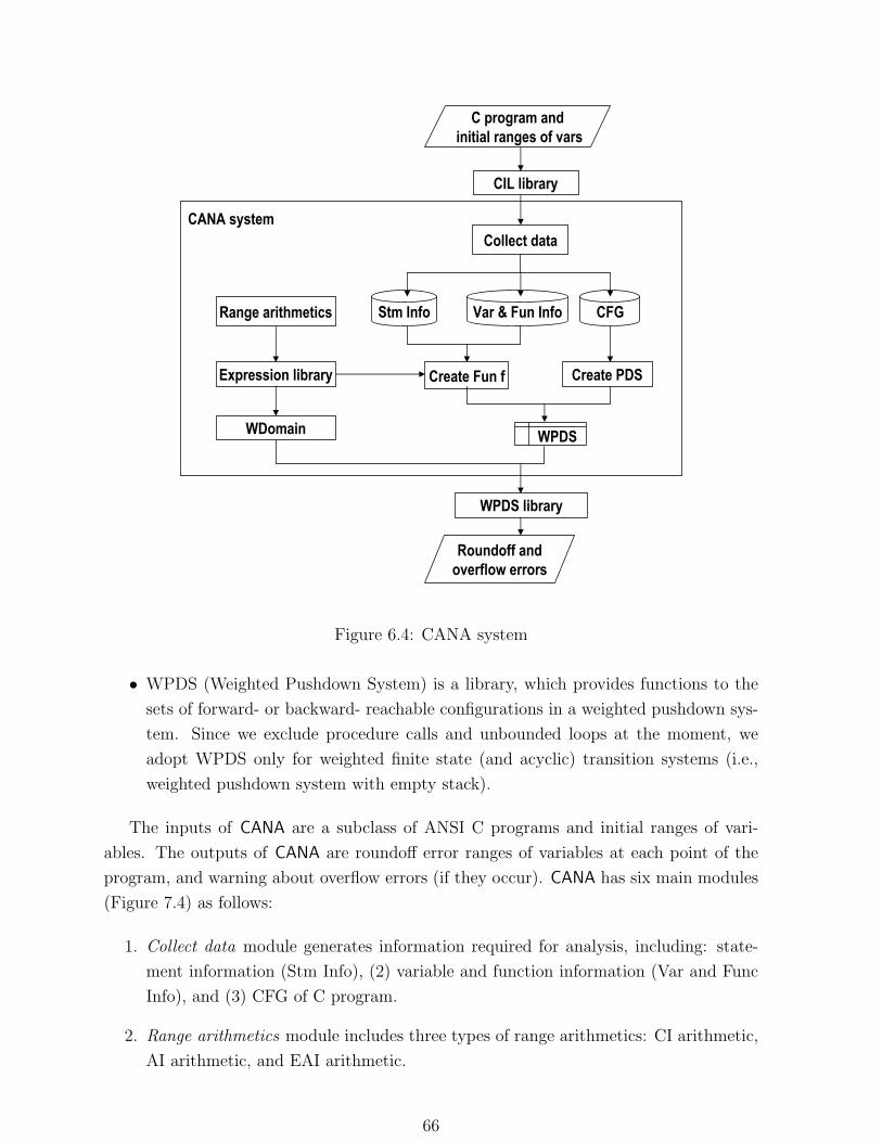
CANA system
CIL library
WPDS library
Roundoff
and overflow errors
C program andinitial ranges of vars
Collect data
Create Fun f
WDomain
Var
& Fun Info
WPDS
Create PDS
CFGStm
InfoRange arithmetics
Expression library
Figure 6.4: CANA system
• WPDS (Weighted Pushdown System) is a library, which provides functions to the
sets of forward- or backward- reachable configurations in a weighted pushdown sys-
tem. Since we exclude procedure calls and unbounded loops at the moment, we
adopt WPDS only for weighted finite state (and acyclic) transition systems (i.e.,
weighted pushdown system with empty stack).
The inputs of CANA are a subclass of ANSI C programs and initial ranges of vari-
ables. The outputs of CANA are roundoff error ranges of variables at each point of the
program, and warning about overflow errors (if they occur). CANA has six main modules
(Figure 7.4) as follows:
1. Collect data module generates information required for analysis, including: state-
ment information (Stm Info), (2) variable and function information (Var and Func
Info), and (3) CFG of C program.
2. Range arithmetics module includes three types of range arithmetics: CI arithmetic,
AI arithmetic, and EAI arithmetic.
66
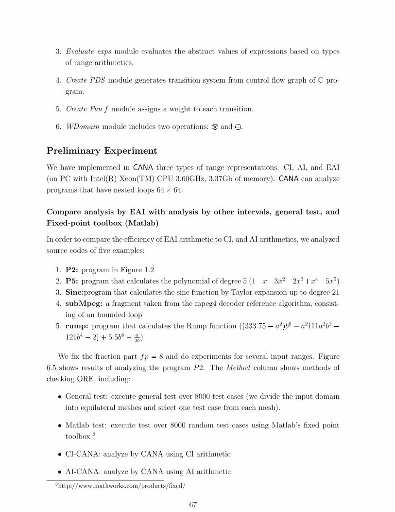
3. Evaluate exps module evaluates the abstract values of expressions based on types
of range arithmetics.
4. Create PDS module generates transition system from control flow graph of C pro-
gram.
5. Create Fun f module assigns a weight to each transition.
6. WDomain module includes two operations: b and `.
Preliminary Experiment
We have implemented in CANA three types of range representations: CI, AI, and EAI
(on PC with Intel(R) Xeon(TM) CPU 3.60GHz, 3.37Gb of memory). CANA can analyze
programs that have nested loops 64 64.
Compare analysis by EAI with analysis by other intervals, general test, and
Fixed-point toolbox (Matlab)
In order to compare the efficiency of EAI arithmetic to CI, and AI arithmetics, we analyzed
source codes of five examples:
1. P2: program in Figure 1.2
2. P5: program that calculates the polynomial of degree 5 (1x3x22x3x45x5)
3. Sine:program that calculates the sine function by Taylor expansion up to degree 21
4. subMpeg: a fragment taken from the mpeg4 decoder reference algorithm, consist-
ing of an bounded loop
5. rump: program that calculates the Rump function (p333.75 a2qb6 a2p11a2b2
121b4 2q 5.5b8 a2b
)
We fix the fraction part fp 8 and do experiments for several input ranges. Figure
6.5 shows results of analyzing the program P2. The Method column shows methods of
checking ORE, including:
• General test: execute general test over 8000 test cases (we divide the input domain
into equilateral meshes and select one test case from each mesh).
• Matlab test: execute test over 8000 random test cases using Matlab’s fixed point
toolbox 3
• CI-CANA: analyze by CANA using CI arithmetic
• AI-CANA: analyze by CANA using AI arithmetic
3http://www.mathworks.com/products/fixed/
67
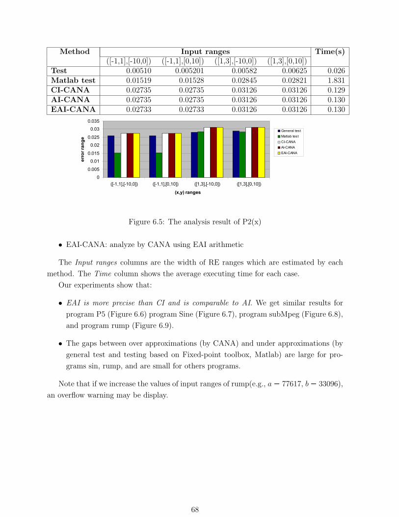
Method Input ranges Time(s)([-1,1],[-10,0]) ([-1,1],[0,10]) ([1,3],[-10,0]) ([1,3],[0,10])
Test 0.00510 0.005201 0.00582 0.00625 0.026Matlab test 0.01519 0.01528 0.02845 0.02821 1.831CI-CANA 0.02735 0.02735 0.03126 0.03126 0.129AI-CANA 0.02735 0.02735 0.03126 0.03126 0.130EAI-CANA 0.02733 0.02733 0.03126 0.03126 0.130P2, f = 8
0
0.005
0.01
0.015
0.02
0.025
0.03
0.035
([-1,1],[-10,0]) ([-1,1],[0,10]) ([1,3],[-10,0]) ([1,3],[0,10])
(x,y) ranges
erro
r ran
ge
General testMatlab testCI-CANAAI-CANAEAI-CANA
Figure 6.5: The analysis result of P2(x)
• EAI-CANA: analyze by CANA using EAI arithmetic
The Input ranges columns are the width of RE ranges which are estimated by each
method. The Time column shows the average executing time for each case.
Our experiments show that:
• EAI is more precise than CI and is comparable to AI. We get similar results for
program P5 (Figure 6.6) program Sine (Figure 6.7), program subMpeg (Figure 6.8),
and program rump (Figure 6.9).
• The gaps between over approximations (by CANA) and under approximations (by
general test and testing based on Fixed-point toolbox, Matlab) are large for pro-
grams sin, rump, and are small for others programs.
Note that if we increase the values of input ranges of rump(e.g., a 77617, b 33096),
an overflow warning may be display.
68
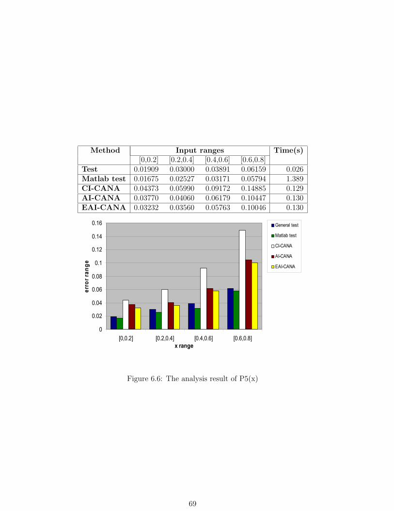
Method Input ranges Time(s)[0,0.2] [0.2,0.4] [0.4,0.6] [0.6,0.8]
Test 0.01909 0.03000 0.03891 0.06159 0.026Matlab test 0.01675 0.02527 0.03171 0.05794 1.389CI-CANA 0.04373 0.05990 0.09172 0.14885 0.129AI-CANA 0.03770 0.04060 0.06179 0.10447 0.130EAI-CANA 0.03232 0.03560 0.05763 0.10046 0.130
0
0.02
0.04
0.06
0.08
0.1
0.12
0.14
0.16
[0,0.2] [0.2,0.4] [0.4,0.6] [0.6,0.8]x range
erro
r ran
ge
General test
Matlab test
CI-CANA
AI-CANA
EAI-CANA
Figure 6.6: The analysis result of P5(x)
69
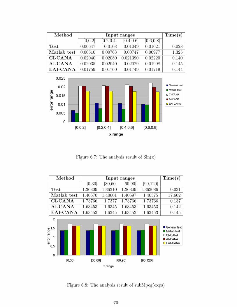
Method Input ranges Time(s)[0,0.2] [0.2,0.4] [0.4,0.6] [0.6,0.8]
Test 0.00647 0.0108 0.01049 0.01021 0.028Matlab test 0.00510 0.00763 0.00747 0.00977 1.325CI-CANA 0.02040 0.02080 0.021390 0.02220 0.140AI-CANA 0.02035 0.02040 0.02029 0.01998 0.145EAI-CANA 0.01759 0.01760 0.01749 0.01719 0.144sin(x), f = 8
0
0.005
0.01
0.015
0.02
0.025
[0,0.2] [0.2,0.4] [0.4,0.6] [0.6,0.8]
x range
erro
r ran
ge
General test
Matlab test
CI-CANA
AI-CANA
EAI-CANA
Figure 6.7: The analysis result of Sin(x)
Method Input ranges Time(s)[0,30] [30,60] [60,90] [90,120]
Test 1.36309 1.36310 1.36309 1.363086 0.031Matlab test 1.40570 1.40601 1.40597 1.40575 17.662CI-CANA 1.73766 1.7377 1.73766 1.73766 0.137AI-CANA 1.63453 1.6345 1.63453 1.63453 0.142EAI-CANA 1.63453 1.6345 1.63453 1.63453 0.145
a part of mpeg decoder, f = 8
0
0.5
1
1.5
2
[0,30] [30,60] [60,90] [90,120]
x range
erro
r ran
ge
General testMatlab testCI-CANAAI-CANAEAI-CANA
Figure 6.8: The analysis result of subMpeg(exps)
70
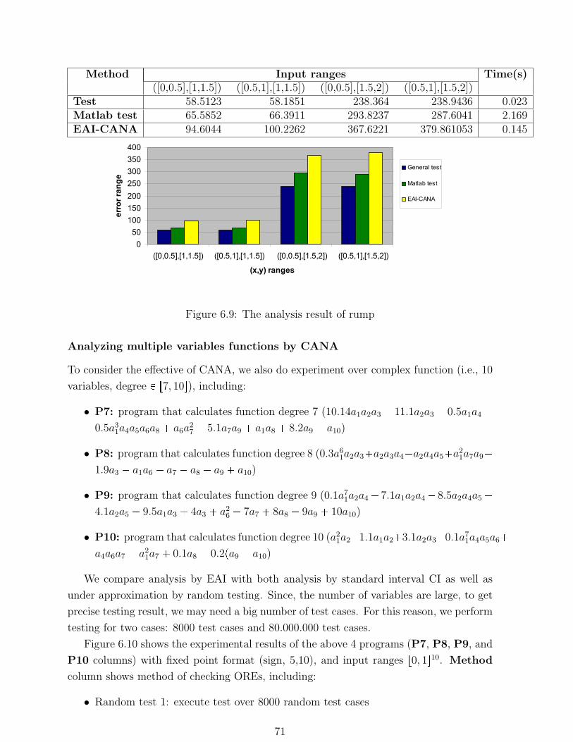
Method Input ranges Time(s)([0,0.5],[1,1.5]) ([0.5,1],[1,1.5]) ([0,0.5],[1.5,2]) ([0.5,1],[1.5,2])
Test 58.5123 58.1851 238.364 238.9436 0.023Matlab test 65.5852 66.3911 293.8237 287.6041 2.169EAI-CANA 94.6044 100.2262 367.6221 379.861053 0.145rump f = 8
050
100150200250300350400
([0,0.5],[1,1.5]) ([0.5,1],[1,1.5]) ([0,0.5],[1.5,2]) ([0.5,1],[1.5,2])
(x,y) ranges
erro
r ran
ge
General test
Matlab test
EAI-CANA
Figure 6.9: The analysis result of rump
Analyzing multiple variables functions by CANA
To consider the effective of CANA, we also do experiment over complex function (i.e., 10
variables, degree P r7, 10s), including:
• P7: program that calculates function degree 7 (10.14a1a2a3 11.1a2a3 0.5a1a4
0.5a31a4a5a6a8 a6a
27 5.1a7a9 a1a8 8.2a9 a10)
• P8: program that calculates function degree 8 (0.3a61a2a3a2a3a4a2a4a5a2
1a7a9
1.9a3 a1a6 a7 a8 a9 a10)
• P9: program that calculates function degree 9 (0.1a71a2a4 7.1a1a2a4 8.5a2a4a5
4.1a2a5 9.5a1a3 4a3 a26 7a7 8a8 9a9 10a10)
• P10: program that calculates function degree 10 (a21a21.1a1a23.1a2a30.1a7
1a4a5a6
a4a6a7 a21a7 0.1a8 0.2pa9 a10)
We compare analysis by EAI with both analysis by standard interval CI as well as
under approximation by random testing. Since, the number of variables are large, to get
precise testing result, we may need a big number of test cases. For this reason, we perform
testing for two cases: 8000 test cases and 80.000.000 test cases.
Figure 6.10 shows the experimental results of the above 4 programs (P7, P8, P9, and
P10 columns) with fixed point format (sign, 5,10), and input ranges r0, 1s10. Method
column shows method of checking OREs, including:
• Random test 1: execute test over 8000 random test cases
71
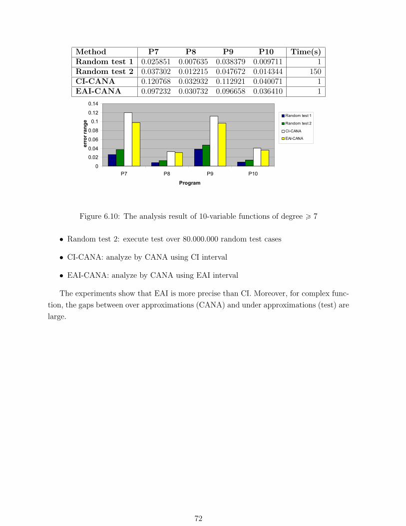
Method P7 P8 P9 P10 Time(s)Random test 1 0.025851 0.007635 0.038379 0.009711 1Random test 2 0.037302 0.012215 0.047672 0.014344 150CI-CANA 0.120768 0.032932 0.112921 0.040071 1EAI-CANA 0.097232 0.030732 0.096658 0.036410 1fp = 10
0
0.02
0.04
0.06
0.08
0.1
0.12
0.14
P7 P8 P9 P10
Program
erro
r ran
ge
Random test 1
Random test 2
CI-CANA
EAI-CANA
Figure 6.10: The analysis result of 10-variable functions of degree ¥ 7
• Random test 2: execute test over 80.000.000 random test cases
• CI-CANA: analyze by CANA using CI interval
• EAI-CANA: analyze by CANA using EAI interval
The experiments show that EAI is more precise than CI. Moreover, for complex func-
tion, the gaps between over approximations (CANA) and under approximations (test) are
large.
72
Chapter 7
Detecting REs based on
Counterexample-guided Narrowing
Static analysis is useful in proving safety properties of ORE problem. But it requires
over approximation in both propagating REs and control flows like conditional branches.
Hence, it may return spurious counterexamples. Fortunately, in our setting, the floating
to fixed point conversion, we can compute the exact RE, whereas there are in general no
ways to compute exact real numbers. Though testing can return exact REs, it cannot
cover all possible inputs. If we are lucky, witness of large REs would be eventually found,
yet most of them may be missed. Another challenging problem is how to reduce the
number of test cases if the input domain is large and the input parameters are many.
A popular approach to deal with spurious counterexamples is counterexample-guided
abstraction refinement (CEGAR) [8]. Inspired by CEGAR, we combine testing and RE
analysis.
This chapter proposes an approach for detecting REs of C programs, which combines
static analysis and testing, and make them refine each other. We call this combination
counterexample-guided narrowing. First, we apply an overflow and roundoff errors analysis
from our previous work [51] which returns an over approximation of REs as an Extended
affine interval (EAI). Fortunately, an EAI represents the relations between the input value
and the RE of the output. These relations can be used to clarify: variables are irrelevant
to REs of the results, variables affect the REs the most, and the ranges of inputs are
most likely to cause the maximum RE. These observations effectively narrow the focus
of test data generation. Second, in case testing does not find a witness of RE violation,
the analysis may over approximate too much. Further, the narrower the input ranges
are, the more precise the analysis result will be. Therefore, with a “divide and conquer”
refinement strategy, we can check the most suspicious part first.
Throughout the chapter, we focus only on roundoff errors. We assume that ORE
analyzer (CANA) does not detect any overflow errors. The rest of this chapter is organized
73
as follows. Section 7.1 presents the overview of the counterexample-guided narrowing
approach. Section 7.2 introduces techniques to improve test data generation. Section 7.3
propose a technique to improve analysis phase by narrowing input domain based on
“divide and conquer” technique. Section 7.4 describes CANAT implementation and reports
experiments.
7.1 Counterexample-guided Narrowing Approach
7.1.1 Observation on RE Analysis
The inputs of an RE analysis consist of
• a C program (with m-input variables) to be analyzed (base b 2),
• a fixed point format psp, ip, fpq,
• an RE threshold θp¡ 0q, and
• a pair of a fixed point range rli, his and an RE range rlmi, hmis with 2fp1
lmi ¤ hmi 2fp1 for each i-th input variable.
We will fix the last three elements as an environment of the RE analysis. We call the
Cartesian product D rl1, h1s rl2m, h2ms an input domain.
Throughout the RE analysis, all ranges are represented as EAIs with 2m noise symbols
(where εi and εmi correspond to noise symbols of the fixed point part and the RE of
values of the i-th input variable). Thus, we coerce input CIs to EAIs by EAI coercion. In
the context of the RE analysis, we denote:
Input domain D rl1, h1s rl2m, h2ms is pv1, . . . , v2mq with vi plihi
2q phili
2qεi.
As notational convention, the analysis result is denoted by an EAI:
pr r0 °2m
i1 riεi
The analysis result r shows extra information about the effects of inputs on r, since
EAI coercions of input ranges and r share common noise symbols. If violations are found
(i.e., EAI projection of r exceeds rθ, θs), we need to check whether they are spurious
by testing. Fortunately, we have useful observations below, which will optimize test data
generation and testing.
• RE bound for each test case: Assume that the valuation of noise symbols for
the test case t pt1, . . . , t2mq is pλ1, . . . , λ2mq, i.e.,
λi
$&%0 if li hi
2tiplihiqphiliq
otherwise
Then, the RE for the input t is bounded by the valuation of r with pλ1, . . . , λ2mq.
74
• Irrelevant noise symbol: If the coefficient of a noise symbol εk is rk r0, 0s, the
noise symbol εk will not affect the RE of result.
• Sensitivity of noise symbols: If |rk| ¤ |rh|, the noise symbol εk affects r more
than εh.
The following example will demonstrate how they affect the testing phases:
Example 33 In the analysis result of Example 31:
• For the test case t pxf , yf , xr, yrq p1, 5, 0, 0q, the valuation of noise symbols is
pε1, ε2, ε3, ε4q p0, 0.5, 0, 0q. The RE bound of t is
r0.031250, 0.031250s r0.26, 0.26s
Therefore, t is not a counterexample.
• Since r2 r0, 0s, ε2 is an irrelevant noise symbol. Hence, v2 (or fixed point part of
y) does not affect RE of rst.
• We have |r1| 0.123091 maxt|r1|, . . . , |r4|u, thus ε1 is the most sensitive noise
symbol. Hence, v1 (or fixed point part of x) affect the RE of rst the most.
The analysis result is helpful to optimize test phase, includes:
• Pre-evaluate test case: if RE bound of a test case t lies in the RE threshold
bound, we need not execute test for t.
• Reduce input ranges: which reduces segments in each input range if correspond-
ing REs are subsumed. Especially, for an irrelevant noise symbol.
• Choice of the number of ticks, which takes more ticks in the input ranges of
more sensitive noise symbols.
7.1.2 Counterexample-guided Narrowing Approach
Our approach are broken down into the following steps. First, we apply an overflow and
roundoff errors analysis from our previous work [51] which returns an over approximation
of REs as an Extended affine interval (EAI). Fortunately, an EAI represents the relations
between the input value and the RE of the output. These relations can be used to clarify:
variables are irrelevant to REs of the results, variables affect the REs the most, and the
ranges of inputs are most likely to cause the maximum RE. These observations effectively
narrow the focus of test data generation.
Second, in case testing does not find a witness of RE violation, the analysis may over
approximate too much. Further, the narrower the input ranges are, the more precise the
analysis result will be. Therefore, with a “divide and conquer” refinement strategy, we
can check the most suspicious part first.
75
7.2 Refining Test Data Generation
Test Data Generation
For an input domain D rl1, h1s rl2m, h2ms, a basic strategy of test data generation
is to divide the input domain into meshes and select one test case from each mesh.
Definition 43 For an interval rl, hs and k ¥ 1,
• the k-random ticks are c1, , ck, and
• the k-periodic ticks are tc, c∆, , c pk 1q∆u,
where ∆ hlk
, and c P rl, l ∆s, c1, , ck P rl, hs are randomly generated.
Remark 8 The ki-random ticks and the ki-periodic ticks are used for random testing and
counterexample-guided narrowing, respectively. For periodic ticks, the offset c is randomly
chosen to avoid overlaps in refinement loops.
Example 34 Let us consider the C program as Fig. 1.2.
• For xf P r1, 3s, let k1 10, then ∆1 p3 p1qq10 0.4. Let c1 0.8, we got
the set of ticks Xf t0.8, 0.4, , 3.8u
• For xr P r25, 25s, let k2 10, then ∆2 p25 p25qq10 0.00625. Let
c2 0.03, we got the set of ticks Xr t0.03, 0.02375, , 0.0265u
• For yf P r10, 10s, let k3 10, then ∆3 p10 p10qq10 2. Let c3 9, we
got the set of ticks Yf t9, 7, , 9u
• For yr P r25, 25s, let k4 10, then ∆4 p25 p25qq10 0.00625. Let
c4 0.028, we got the set of ticks Yr t0.028, 0.02175, , 0.0285u
Hence, the set of test data is T Xf Yf Xr Yr. E.g., For test case t1
p0.8,9,0.03,0.028q, the input of fixed point program is px, yq p0.8,9q; the
input of floating point program is px, yq p0.83,9.028q.
For an input domain D rl1, h1s rl2m, h2ms, all combinations of ki-ticks of
rli, his for i ¤ 2m are the set of test data. Then, we execute a program in two ways: with
floating point arithmetic and fixed point arithmetic. The difference between them is a
true RE. However, the number of test data grows with the power of the 2m-th degree.
76
7.2.1 Range Reduction
For two ranges rl1, h1s, rl2, h2s, we denote rl1, h1s ¤ rl2, h2s if u ¤ v for each u P rl1, h1s
and v P rl2, h2s (i.e., h1 ¤ l2). Reducing input range is executed based on the observation
as the following lemma.
Lemma 2 Assume 0 R ru, vs. Then,
• rv,us ¤ ru, vsruv, u
vs ¤ ru, vs if 0 u ¤ v
• ru, vs ¤ ru, vsr vu, v
us ¤ rv, us if u ¤ v 0
This lemma means that if 0 R rui, vis ri we can ignore test data with corresponding
noise symbol εi in rui
vi, ui
vis (resp. r vi
ui, vi
uis) for 0 ui ¤ vi (resp. ui ¤ vi 0). The
reason for this is that the true REs for test data with εi in rui
vi, ui
vis (resp. r vi
ui, vi
uis)
are bounded by the valuations when a noise symbol εi is either 1 or 1 whatever a true
coefficient has a value in rui, vis.
In a special case ui vi 0, a valuation of εi does not matter. Thus, only a valuation
with 0 is considered.
From observations above we reduce the input domain D to two input domains Dmax
(which contain an input that causes the maximum RE) and Dmin (which contain an input
that causes the minimum RE) without loosing opportunities to find test cases that cause
violation of REs.
Definition 44 For an input domain
D
p l1h1
2 h1l1
2ε1q p
l2mh2m
2 h2ml2m
2ε2mq and the analysis result
pr ru0, v0s 2m
i1
rui, visεi,
the subdomain Dmax of D is
pl1 h1
2
h1 l12
ε1q pl2m h2m
2
h2m l2m
2ε2mq
where
εi
$'''''&'''''%r |ui||vi|
, 1s if 0 ui ¤ vi
r1, |vi||ui|s if ui ¤ vi 0
r0, 0s if ui vi 0
r1, 1s otherwise
and the subdomain Dmin is
pl1 h1
2
h1 l12
ε1q pl2m h2m
2
h2m l2m
2ε2mq
77
where
εi
$'''''&'''''%r1, |ui|
|vi|s if 0 ui ¤ vi
r |vi||ui|
, 1s if ui ¤ vi 0
r0, 0s if ui vi 0
r1, 1s otherwise
An EAI pr r0 °2m
i1 riεi is maximum (resp. minimum) if each of elements r0 and
riεi is maximized (resp. minimized). Thus the maximal (resp. minimal) RE will occur
among valuations of εi in ruv, 1s (resp. r1,uvs) if 0 u ¤ v, and in r1,vus
(resp. rvu, 1s) if u ¤ v 0. Therefore, from Lemma 2, we obtain the next theorem.
Theorem 4 If there exists a counterexample in D, then there exists a counterexample in
Dmax YDmin.
Example 35 By observation of analysis result r in Example 31, we can find Dmax of the
input domain D is
pr1, 1s r2, 2sε1q pr10, 10sε2q pr25, 25sε3q pr2
5, 25sε4q
with ε1 r1, 1s, ε2 r0, 0s, ε3 r0.63589, 1s, and ε4 r1,1s. Hence, Dmax is
projected to
r1, 3s r0, 0s r0.019872, 0.03125s r0.03125,0.03125s.
Hence, we can conclude that the input with yf 0 and yr 0.03125 will cause the
maximum RE.
7.2.2 More Ticks for more Sensitive Noise Symbols
We need a strategy to setting ticks for each initial ranges in input domain. A bad strategy
of setting ticks will create several test cases which cause similar REs and all of them lie
within RE threshold bound. Testing over these test cases are not needed.
Analysis result r shows the effects of noise symbols to the REs. A larger coefficient of
a noise symbol causes stronger effect on the RE of the result. For example, the variable
corresponding to dominant noise symbol will strongly affect REs, in other words, the
changing of this variable causes the changing of RE the most. Therefore, setting more
ticks on the initial range of this variables can lead the test cases to various REs. Based
on this observation, our basic idea is, in input domains Dmin, Dmax, the initial range of
variables which are predicated strongly affect REs will be set more ticks than other initial
ranges. The strategy of setting number of ticks is then depending on coefficients of noise
symbols in analysis result as follows:
78
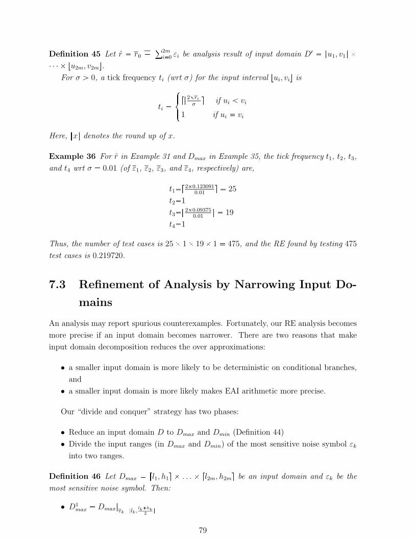
Definition 45 Let r r0 °2m
i0 εi be analysis result of input domain D1 ru1, v1s
ru2m, v2ms.
For σ ¡ 0, a tick frequency ti (wrt σ) for the input interval rui, vis is
ti
$&%r|2ri|
σs if ui vi
1 if ui vi
Here, rxs denotes the round up of x.
Example 36 For r in Example 31 and Dmax in Example 35, the tick frequency t1, t2, t3,
and t4 wrt σ 0.01 (of ε1, ε2, ε3, and ε4, respectively) are,
t1r20.123091
0.01s 25
t21
t3r20.09375
0.01s 19
t41
Thus, the number of test cases is 25 1 19 1 475, and the RE found by testing 475
test cases is 0.219720.
7.3 Refinement of Analysis by Narrowing Input Do-
mains
An analysis may report spurious counterexamples. Fortunately, our RE analysis becomes
more precise if an input domain becomes narrower. There are two reasons that make
input domain decomposition reduces the over approximations:
• a smaller input domain is more likely to be deterministic on conditional branches,
and
• a smaller input domain is more likely makes EAI arithmetic more precise.
Our “divide and conquer” strategy has two phases:
• Reduce an input domain D to Dmax and Dmin (Definition 44)
• Divide the input ranges (in Dmax and Dmin) of the most sensitive noise symbol εk
into two ranges.
Definition 46 Let Dmax rl1, h1s . . . rl2m, h2ms be an input domain and εk be the
most sensitive noise symbol. Then:
• D1max Dmax|vkrlk,
lkhk2
s
79
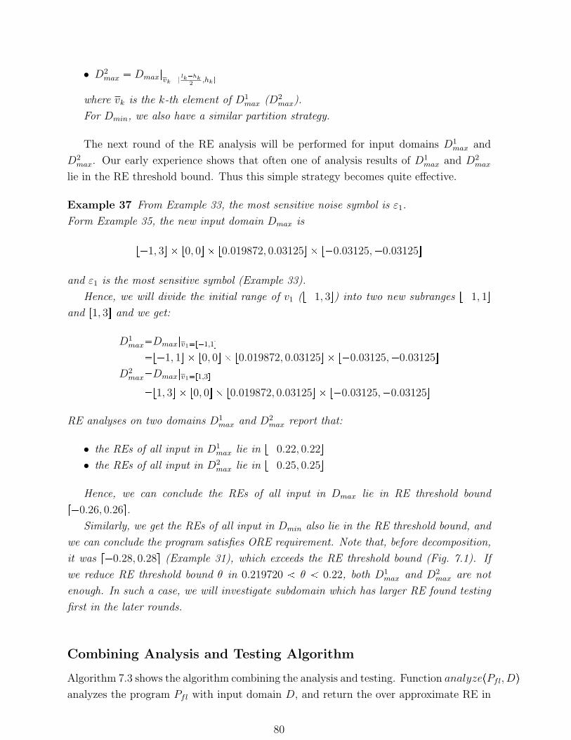
• D2max Dmax|vkr
lkhk2
,hks
where vk is the k-th element of D1max (D2
max).
For Dmin, we also have a similar partition strategy.
The next round of the RE analysis will be performed for input domains D1max and
D2max. Our early experience shows that often one of analysis results of D1
max and D2max
lie in the RE threshold bound. Thus this simple strategy becomes quite effective.
Example 37 From Example 33, the most sensitive noise symbol is ε1.
Form Example 35, the new input domain Dmax is
r1, 3s r0, 0s r0.019872, 0.03125s r0.03125,0.03125s
and ε1 is the most sensitive symbol (Example 33).
Hence, we will divide the initial range of v1 (r1, 3s) into two new subranges r1, 1s
and r1, 3s and we get:
D1maxDmax|v1r1,1s
r1, 1s r0, 0s r0.019872, 0.03125s r0.03125,0.03125s
D2maxDmax|v1r1,3s
r1, 3s r0, 0s r0.019872, 0.03125s r0.03125,0.03125s
RE analyses on two domains D1max and D2
max report that:
• the REs of all input in D1max lie in r0.22, 0.22s
• the REs of all input in D2max lie in r0.25, 0.25s
Hence, we can conclude the REs of all input in Dmax lie in RE threshold bound
r0.26, 0.26s.
Similarly, we get the REs of all input in Dmin also lie in the RE threshold bound, and
we can conclude the program satisfies ORE requirement. Note that, before decomposition,
it was r0.28, 0.28s (Example 31), which exceeds the RE threshold bound (Fig. 7.1). If
we reduce RE threshold bound θ in 0.219720 θ 0.22, both D1max and D2
max are not
enough. In such a case, we will investigate subdomain which has larger RE found testing
first in the later rounds.
Combining Analysis and Testing Algorithm
Algorithm 7.3 shows the algorithm combining the analysis and testing. Function analyzepPfl, Dq
analyzes the program Pfl with input domain D, and return the over approximate RE in
80
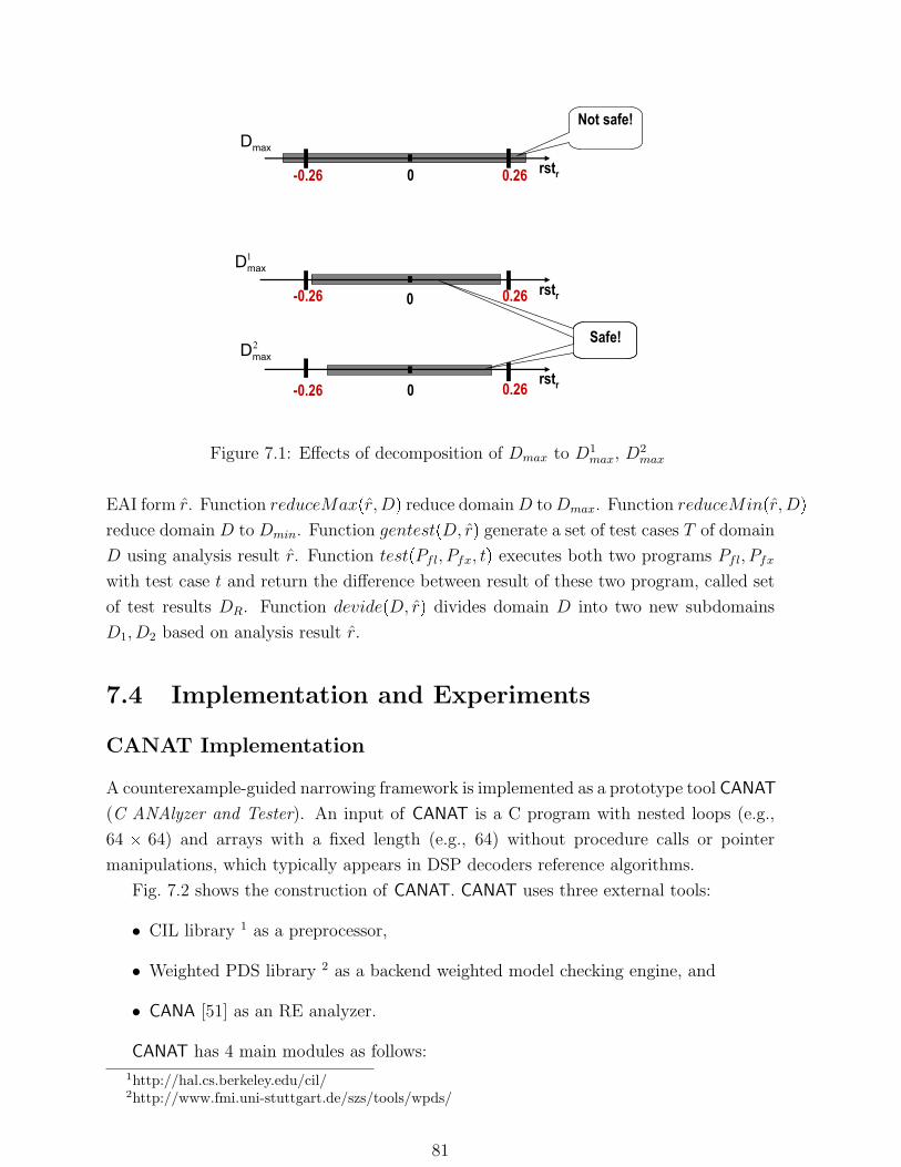
-0.26 0.260 rstr
-0.26 0.260 rstr
-0.26 0.260rstr
Not safe!
Safe!
1maxD
2maxD
maxD
Figure 7.1: Effects of decomposition of Dmax to D1max, D2
max
EAI form r. Function reduceMaxpr, Dq reduce domain D to Dmax. Function reduceMinpr, Dq
reduce domain D to Dmin. Function gentestpD, rq generate a set of test cases T of domain
D using analysis result r. Function testpPfl, Pfx, tq executes both two programs Pfl, Pfx
with test case t and return the difference between result of these two program, called set
of test results DR. Function devidepD, rq divides domain D into two new subdomains
D1, D2 based on analysis result r.
7.4 Implementation and Experiments
CANAT Implementation
A counterexample-guided narrowing framework is implemented as a prototype tool CANAT
(C ANAlyzer and Tester). An input of CANAT is a C program with nested loops (e.g.,
64 64) and arrays with a fixed length (e.g., 64) without procedure calls or pointer
manipulations, which typically appears in DSP decoders reference algorithms.
Fig. 7.2 shows the construction of CANAT. CANAT uses three external tools:
• CIL library 1 as a preprocessor,
• Weighted PDS library 2 as a backend weighted model checking engine, and
• CANA [51] as an RE analyzer.
CANAT has 4 main modules as follows:
1http://hal.cs.berkeley.edu/cil/2http://www.fmi.uni-stuttgart.de/szs/tools/wpds/
81
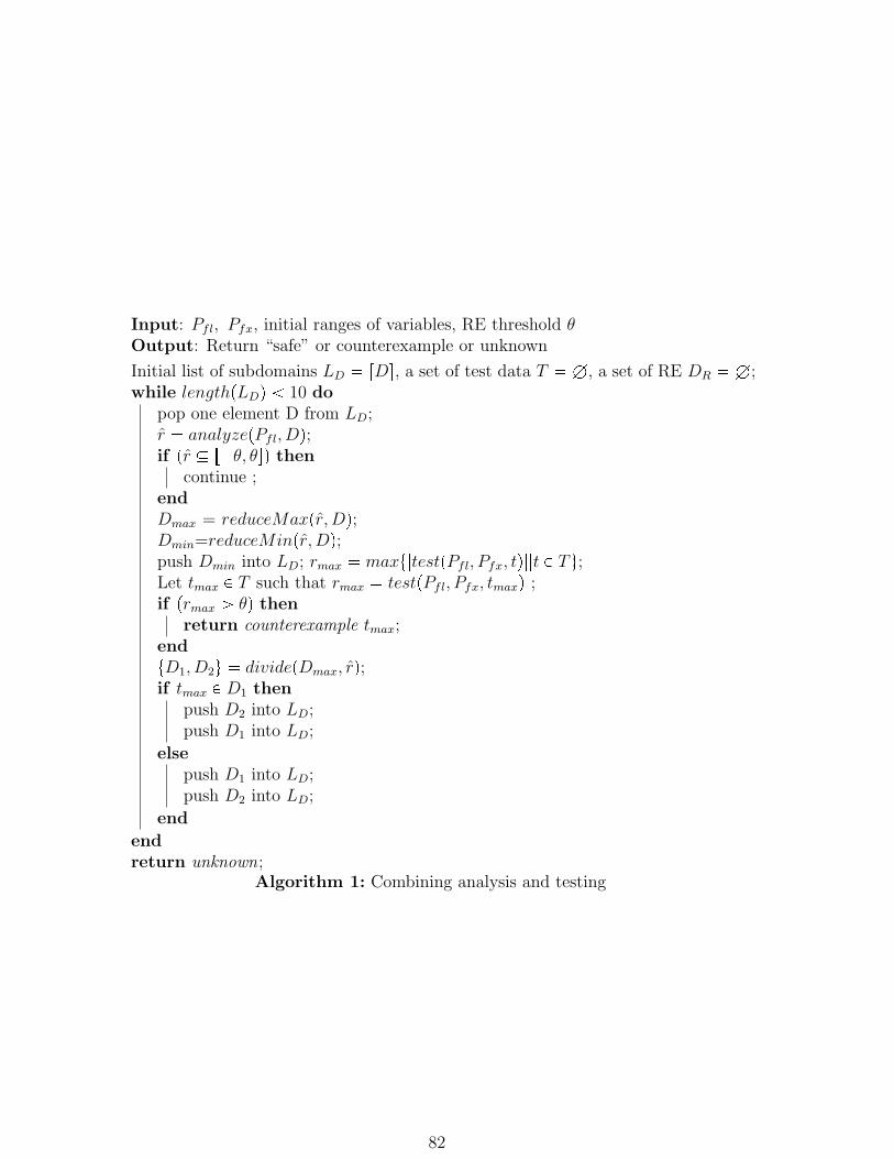
Input: Pfl, Pfx, initial ranges of variables, RE threshold θOutput: Return “safe” or counterexample or unknown
Initial list of subdomains LD rDs, a set of test data T H, a set of RE DR H;while lengthpLDq 10 do
pop one element D from LD;r analyzepPfl, Dq;if pr rθ, θsq then
continue ;endDmax = reduceMaxpr, Dq;Dmin=reduceMinpr, Dq;push Dmin into LD; rmax maxt|testpPfl, Pfx, tq||t P T u;Let tmax P T such that rmax testpPfl, Pfx, tmaxq ;if prmax ¡ θq then
return counterexample tmax;endtD1, D2u dividepDmax, rq;if tmax P D1 then
push D2 into LD;push D1 into LD;
elsepush D1 into LD;push D2 into LD;
end
endreturn unknown;
Algorithm 1: Combining analysis and testing
82
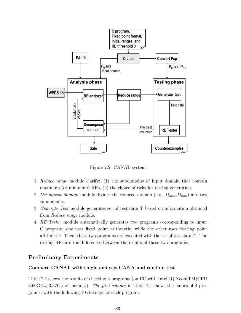
CIL lib
RE analyzer
Decomposedomain
Generate test
RE Tester
Counterexamples
C program,Fixed point format, Initial ranges, andRE threshold θ
Analysis phase Testing phase
Pflt
andinput domain
The best test case
Test data
Subd
omain
choic
e
Safe
EAI lib
WPDS lib
Convert Fxp
Pflt
and Pfxp
Reduce range
Figure 7.2: CANAT system
1. Reduce range module clarify: (1) the subdomains of input domain that contain
maximum (or minimum) REs, (2) the choice of ticks for testing generation.
2. Decompose domain module divides the reduced domain (e.g., Dmax,Dmin) into two
subdomains.
3. Generate Test module generates set of test data T based on information obtained
from Reduce range module.
4. RE Tester module automatically generates two programs corresponding to input
C program, one uses fixed point arithmetic, while the other uses floating point
arithmetic. Then, these two programs are executed with the set of test data T . The
testing REs are the differences between the results of these two programs.
Preliminary Experiments
Compare CANAT with single analysis CANA and random test
Table 7.1 shows the results of checking 4 programs (on PC with Intel(R) Xeon(TM)CPU
3.60GHz, 3.37Gb of memory). The first column in Table 7.1 shows the names of 4 pro-
grams, with the following 40 settings for each program.
83
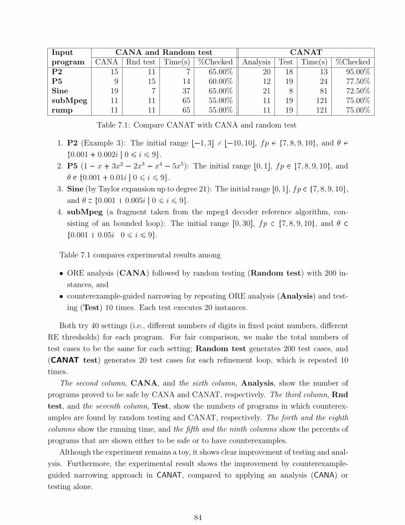
Input CANA and Random test CANATprogram CANA Rnd test Time(s) %Checked Analysis Test Time(s) %CheckedP2 15 11 7 65.00% 20 18 13 95.00%P5 9 15 14 60.00% 12 19 24 77.50%Sine 19 7 37 65.00% 21 8 81 72.50%subMpeg 11 11 65 55.00% 11 19 121 75.00%rump 11 11 65 55.00% 11 19 121 75.00%
Table 7.1: Compare CANAT with CANA and random test
1. P2 (Example 3): The initial range r1, 3s r10, 10s, fp P t7, 8, 9, 10u, and θ P
t0.001 0.002i | 0 ¤ i ¤ 9u.
2. P5 (1 x 3x2 2x3 x4 5x5): The initial range r0, 1s, fp P t7, 8, 9, 10u, and
θ P t0.001 0.01i | 0 ¤ i ¤ 9u.
3. Sine (by Taylor expansion up to degree 21): The initial range r0, 1s, fp P t7, 8, 9, 10u,
and θ P t0.001 0.005i | 0 ¤ i ¤ 9u.
4. subMpeg (a fragment taken from the mpeg4 decoder reference algorithm, con-
sisting of an bounded loop): The initial range r0, 30s, fp P t7, 8, 9, 10u, and θ P
t0.001 0.05i | 0 ¤ i ¤ 9u.
Table 7.1 compares experimental results among
• ORE analysis (CANA) followed by random testing (Random test) with 200 in-
stances, and
• counterexample-guided narrowing by repeating ORE analysis (Analysis) and test-
ing (Test) 10 times. Each test executes 20 instances.
Both try 40 settings (i.e., different numbers of digits in fixed point numbers, different
RE thresholds) for each program. For fair comparison, we make the total numbers of
test cases to be the same for each setting; Random test generates 200 test cases, and
(CANAT test) generates 20 test cases for each refinement loop, which is repeated 10
times.
The second column, CANA, and the sixth column, Analysis, show the number of
programs proved to be safe by CANA and CANAT, respectively. The third column, Rnd
test, and the seventh column, Test, show the numbers of programs in which counterex-
amples are found by random testing and CANAT, respectively. The forth and the eighth
columns show the running time, and the fifth and the ninth columns show the percents of
programs that are shown either to be safe or to have counterexamples.
Although the experiment remains a toy, it shows clear improvement of testing and anal-
ysis. Furthermore, the experimental result shows the improvement by counterexample-
guided narrowing approach in CANAT, compared to applying an analysis (CANA) or
testing alone.
84
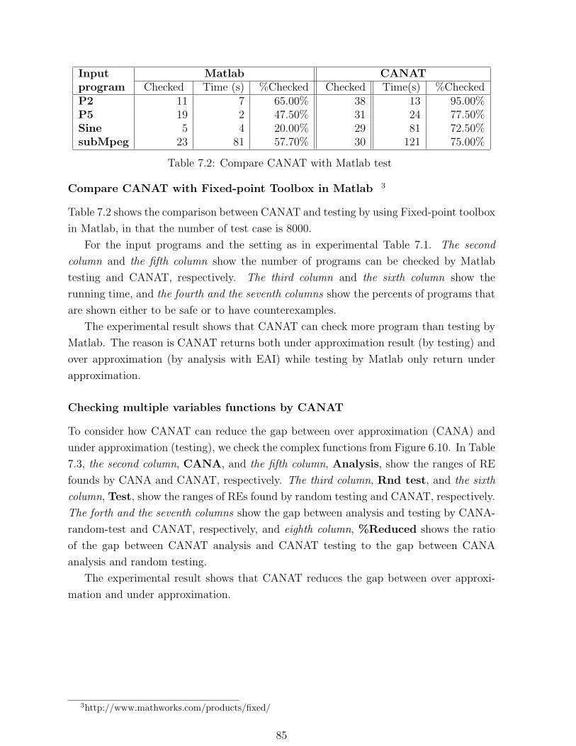
Input Matlab CANATprogram Checked Time (s) %Checked Checked Time(s) %CheckedP2 11 7 65.00% 38 13 95.00%P5 19 2 47.50% 31 24 77.50%Sine 5 4 20.00% 29 81 72.50%subMpeg 23 81 57.70% 30 121 75.00%
Table 7.2: Compare CANAT with Matlab test
Compare CANAT with Fixed-point Toolbox in Matlab 3
Table 7.2 shows the comparison between CANAT and testing by using Fixed-point toolbox
in Matlab, in that the number of test case is 8000.
For the input programs and the setting as in experimental Table 7.1. The second
column and the fifth column show the number of programs can be checked by Matlab
testing and CANAT, respectively. The third column and the sixth column show the
running time, and the fourth and the seventh columns show the percents of programs that
are shown either to be safe or to have counterexamples.
The experimental result shows that CANAT can check more program than testing by
Matlab. The reason is CANAT returns both under approximation result (by testing) and
over approximation (by analysis with EAI) while testing by Matlab only return under
approximation.
Checking multiple variables functions by CANAT
To consider how CANAT can reduce the gap between over approximation (CANA) and
under approximation (testing), we check the complex functions from Figure 6.10. In Table
7.3, the second column, CANA, and the fifth column, Analysis, show the ranges of RE
founds by CANA and CANAT, respectively. The third column, Rnd test, and the sixth
column, Test, show the ranges of REs found by random testing and CANAT, respectively.
The forth and the seventh columns show the gap between analysis and testing by CANA-
random-test and CANAT, respectively, and eighth column, %Reduced shows the ratio
of the gap between CANAT analysis and CANAT testing to the gap between CANA
analysis and random testing.
The experimental result shows that CANAT reduces the gap between over approxi-
mation and under approximation.
3http://www.mathworks.com/products/fixed/
85
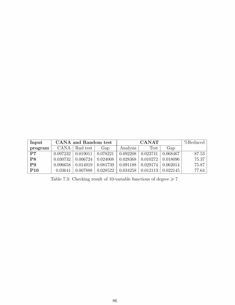
Input CANA and Random test CANAT %Reducedprogram CANA Rnd test Gap Analysis Test GapP7 0.097232 0.019011 0.078221 0.092208 0.023741 0.068467 87.53P8 0.030732 0.006724 0.024008 0.028368 0.010272 0.018096 75.37P9 0.096658 0.014919 0.081739 0.091188 0.029174 0.062014 75.87P10 0.03641 0.007888 0.028522 0.034258 0.012113 0.022145 77.64
Table 7.3: Checking result of 10-variable functions of degree ¥ 7
86
Chapter 8
Related Work
The ORE analysis has been attracted extensive attention of research in the numerical
analysis recently. Several different approaches has been proposed to deal with the problem
of roundoff and overflow problems. In this chapter, we give a survey of recent related works
on the topics of ORE analysis.
The ORE problems are one of the central issues in the numerical analysis [17, 22].
There are lots of works on mathematical reasoning to estimate OREs [21, 22], and there
is a well-known methodology for the precise addition of floating numbers, which cancels
the effect of REs [33]. It is extended to the precise multiplication [53], and recently verified
numerical computation is evolving.
Our focus is more on static detections of OREs of programs, and we omit huge refer-
ences of these areas, which are beyond scope of the thesis.
Range representations of real numbers
Due to REs, we need to evaluate values of real numbers by some representation of ranges.
They are classically classified into:
• Interval, which is the Cartesian product of one dimensional intervals [2, 47].
• Octagon, which is surrounded by either vertical, horizontal, or diagonal lines [46].
• Polyhedra, which is represented as the conjunction of linear inequalities [10]. Re-
cently, its refinement SubPolyhedra was proposed [36] by reducing deduction rules
among linear inequalities, yet preserving expressiveness.
We are more focus on intervals, and we call a range described by a pair of the lowest
and the highest value by a classical interval (CI). CI is generalized to allow swapping of
boundaries [23].
87
By introducing noise symbols, which preserve dependency of uncertainty, Affine in-
terval (AI) has been proposed [61, 62]. Later, we will see how AI is applied as over
approximation for ORE analyses.
Extended Affine interval (EAI) has proposed for under approximation, based on the
mean value theorem and Kaucher arithmetic [27]. EAI replaces real coefficients of AI
with CI coefficients. We apply this idea for over approximation of ORE analysis.
Numerical Constraint Solvers
Recently, several tools have been developed as variations of SMT to solve non-linear
numerical constrains. For instance,
• iSAT [16], which evaluates non-linear operations to interval constraints by over
approximation.
• minismt [64], which covers specific irrationals, such as rational numbers and roots of
small integers. They are symbolically represented and its bounded search is encoded
as CNF.
• a tool for Simulink/Stateflow models [30], which applied a variation of polyhedra,
called the bounded vertex representation for under approximation.
Ganai and Ivancic [18] introduced a new method to face with decision problems in-
volving non-linear constraints on bounded integers. Each nonlinear operation is encoded
into a Boolean combination of linear arithmetic constraints based on CORDIC algorithm.
Then, the linearized formula will be input of a DPLL-style Interval Search Engine that
explores various combination of interval bounds using a SMT solver.
To solve an interval constraint, they divide the input ranges to smaller ranges, which
is similar to ours. Adding to the difference of target domains (i.e., bounded integers
and floating/fixed point numbers), the differences are, (1) we use EAI instead of CI, (2)
combination with testing, and (3) weighted model checking instead of (SMT) solver.
To solve dataflow equations over infinite domains, such as numerical constraints (mostly
on integers), several algorithms are proposed in the context of weighted pushdown model
checking [25, 20, 37, 48].
The library Apron of numerical abstract domains is also freely available [29].
ORE analysis
For a static analysis, we need a concrete semantics. We obey the semantics of propagation
of OREs to [39].
There are three kinds of OREs, caused by:
88
• real numbers to floating point numbers conversion,
• real numbers to fixed point numbers conversion, and
• floating point numbers to fixed point numbers conversion.
ORE analysis are mainly investigated for the first and the third.
For the real numbers to floating point numbers conversion, ORE analysis adapt
AI [26, 40] (which introduced widening operators to handle loops), except that the octagon
abstract domain is used in [45].
They are implemented and showed experimental results. FLUCTUAT is presented
in [26] and [45] showed a case study on an embedded avionics software. The technique of
[40] is further applied on TMS320 C3X assembler programs [41].
These ORE analyses are over approximation, and easily cause false positives. An ORE
analysis with under approximation is proposed based on the mean value theorem and
Kaucher arithmetic [27], to sandwich OREs from both sides. However, strictly speaking,
this under approximation is for real number variables rather than floating point number
variables.
The floating point numbers to fixed point numbers conversion typically appears in
hard-wired algorithms and/or embedded systems. Apart from difficulties in hardware
encoding difficulties [3, 5, 31, 32, 44, 58, 59], there are strong demand to solve ORE
problems.
For the floating point numbers to fixed point numbers conversion, Fang, et.al. [13,
14, 15] proposed an ORE analysis based on AI, intended for DSP applications. We are
facing on the same problem, but with different intervals, EAI. In our implementation, we
adapted a sophisticated weighted model checking, whereas they adapt direct bit-vector
encoding. For scalability, they also applied probabilistic reduction of the search space.
Thanks to the problem nature, we can examine OREs by testing, since we can compute
both floating point numbers and fixed point numbers. [63] showed a such testing tool.
We further combined an ORE analysis and testing by a counter example guided nar-
rowing approach, which refines the focus of testing and avoid spurious counterexamples
in an early stage.
Refining analyses and testing
As general setting of static estimation, recently the refinement loop of analyses and testing
is extensively investigated.
Counterexample Guided Abstraction-refinement (CEGAR) [8] is widely applied method-
ology, in which the initial abstract model typically nondeterministic control structures for
89
conditional branches. When (possible spurious) counter examples are found, symbolic
techniques refine the model by hooking more deterministic behavior.
Proofs from Tests [4] presented an algorithm DASH to check if a program satisfies
a safety property. It uses only test generation, and it refines and maintains a sound
program abstraction as a consequence of failed test generation operations. This enables
us a light-weight refinement loop with neither any extra theorem prover calls nor any
global may-alias information.
Our methodology of counter example guided narrowing tries to refine the focus of
testing based on ORE analysis results. Fortunately, by the nature of EAI, ORE analysis
results tell us which input parameter is dominant for REs. By using this information, we
can effectively focus on the most problematic point.
90
Chapter 9
Conclusions
Motivated by automatically detecting OREs of hardware systems, this thesis proposes a
novel interval-valued approach for representing and reasoning about OREs. We concen-
trate on the overflow and roundoff errors between floating point arithmetic and fixed point
arithmetic, which are frequently troublesome in DSP decoders when a reference algorithm
with floating point numbers is converted to a hard-wired logic with fixed point numbers.
It contributes several techniques for improving interval computations, automatically esti-
mating OREs with high precision. This chapter reviews the main contributions, and then
discusses about future research.
9.1 Summary of the Thesis
First of all, our contributions are summarized as follows:
• In Chapter 4, two new range representations were propose, named extended affine
interval (EAI) and positive-noise affine interval (PAI). EAI is extended from AI by
assigning for each noise symbol a CI coefficient. By this representation, EAI has two
main advantages over current range representations (CI and AI). First, EAI is more
precise than CI because EAI can store information about sources of uncertainty as
noise symbol, whereas CI cannot. Second, EAI forms are more compact than AI
forms. This is because EAI arithmetic does not introduce new noise symbols, while
AI arithmetic does. PAI is another way to extend AI in that the noise symbols are
set to lie in r0, 1s (instead of r1, 1s). Thus, PAI nonlinear operations are designed
to reduce over approximation (compare to AI and EAI).
• In Chapter 6, the ORE analysis is treat as a weighted model checking problem.
In that, range representations (i.e., CI, AI, and EAI) are used in the abstraction
of OREs. To avoid widening (which often leads to large over approximation), we
restrict to a subclass C program which have only bounded loops. The model of the
program becomes acyclic model by unfolding loops. Thus, the weigh domain can
91
be generated by an on-the-fly manner and satisfies the descending chain condition.
Based on this approach, a static analysis tool CANA for overflow and roundoff error
analysis of subclass C programs was implemented. Although our experiments were
performed on small examples, the result is encouraging that EAI is more precise
than CI and is comparable to AI.
• In Chapter 7, we proposed an approach for finding both under-approximation and
over approximation of RE ranges. In particular, the under-approximation is com-
puted by testing method and over approximation is computed by analysis method.
Further, static analysis and testing are combined, to make them refine each other
(called counterexample-guided narrowing). The refinement loop (i.e., testing + anal-
ysis) is repeated to refined both testing phase and analysis phase. Thus, the result
will be more precise than either testing or static analysis alone. Note that, this ap-
proach can not be applied for detecting REs between real number and floating point
numbers (or fixed point numbers) because there is no way to automatically test real
algorithm exactly. Using the proposed approach, a prototype tool named CANAT,
is implemented based on CANA. We would like to emphasize that, although our ex-
periments are still small, the results are encouraging and show potential usefulness
in practice.
9.2 Future Work
For future work, we plan to consider the following issues: For future works, one obstacle is
the scalability of CANA and CANAT. We are optimistic since DSP algorithms (e.g., digital
video compression [54]) are often compositional. They typically consist of sequences of
computations with fixed-length arrays and bounded loops. Therefore, we can divide the
algorithm to small fragments and check each separately.
Second, widening operator design. Currently, we did not introduce widening operators,
but first focus on precision of ORE detection. (For instance, the widening operator [26]
leads to inevitably lose precision a lot.) Its drawback is that the class of target programs
has strong limitation, though it seems enough for the core part of DSP encoders/decoders.
We are also interested in an automatic correction of a program to improve with less
OREs. For instance, in [43], there are several techniques to automatically improve nu-
merical precision, such as:
• swapping the order of arithmetic operations,
• explicit shifting of the order of magnitude, and
• symbolic executions.
92

Our ORE analyzer, CANA, can generate the information about range values of fixed-
point numbers and their RE at each point of the program. There information is helpful
information to automatic source code correction.
93
Bibliography
[1] Aho, A.V., Sethi, R., Ullman, J.D.: Compilers: Principles, Techniques, and Tools.
Addison-Wesley (1986)
[2] Alefeld, G. and Herzberger, J.: Introduction to Interval Computations. Academic
Press, N.Y. (1983)
[3] Banerjee, P., Bagchi, D., Haldar, M., Nayak, A., Kim, V., and Uribe, R.: Automatic
Conversion of floating-point MATLAB Programs into fixed-point FPGA Based Hard-
ware Design. In Proc. of the 11th Annual IEEE Symposium on Field-Programmable
Custom Computing Machines, pp. 263, IEEE Computer Society (2003)
[4] Beckman, N.E., Nori, A.V., Rajamani, S.K., Simmons, R.J., Tetali, S.D., Thakur,
A.V.: Proofs from Tests. In IEEE Transactions on Software Engineering: Special
Issue on the ISSTA 2008 Best Papers, IEEE Computer Society (2008)
[5] Belanovic, P. and Rupp, M.: Automated Floating-Point to Fixed-Point Conversion
with the Fixify Environment. In Proc. of the 16th IEEE International Workshop on
Rapid System Prototyping, pp. 172 - 178, IEEE Computer Society (2007)
[6] Brown, C. W., Davenport, J. H.: The complexity of quantifier elimination and cylin-
drical algebraic decomposition. In Proc. of the 2007 International Symposium on
Symbolic and algebraic computation, pp. 54 - 60, ACM (2007)
[7] Clarke, E. Grumberg, O., and Peled, D. A.: Model checking. MIT Press, L.D. (1999)
[8] Clarke, E., Grumberg, O., Jha, S., Lu, Y., and Veith, H.: Counterexample-guided
abstraction refinement. In Proc. of the 12th International Conference on Computer
Aided Verification , pp. 154-169, Springer-Verlag (2000)
[9] Cousot, P. and Cousot, R.: Abstract interpretation: a unified lattice model for static
analysis of programs by construction or approximation of fixpoints. In Proc. of the
4th ACM SIGACT-SIGPLAN Symposium on Principles of Programming Languages,
pp. 238-252, ACM (1977)
94
[10] Cousot, P. and Halbwachs, N.: Automatic discovery of linear restraints among vari-
ables of a program. In Proc. of the 5th ACM SIGPLAN-SIGACT Symposium on
Principles of Programming Languages, pp.84-96, ACM (1978)
[11] Dijkstra, E.W.: A discipline of programming. Series in Automatic Computation.
Prentice Hall (1976)
[12] Emerson, E. A.: Temporal and modal logic. Handbook of Theoretical Computer
Science, MIT (1990)
[13] Fang, C.F., Rutenbar, R.A., and Chen, T.: Fast, accurate static analyis for fixed-
point finite precision effects in DSP designs. In Proc. of the International Conference
on Computer Aided Design, pp. 275-282, IEEE Computer Society (2003)
[14] Fang, C.F.: Probabilistic Interval-Valued Computation: Representing and Reasoning
about Uncertainty in DSP and VLSI Design. Ph. D. Diserration, Depterment of
Electrical and Computer Engineering, Carnegie Mellon University (2005)
[15] Fang, C.F., Rutenbar, R.A., Puschel, M. and Chen, T.: Toward efficient static anal-
ysis of finite-precision effects in DSP applications via Affine arithmetic modeling. In
Proc. of Design Automation Conference, pp. 496-501, ACM Press (2003)
[16] Franzle, M., Herde, C., Teige, T., Ratschan, S., and Schubert, T.: Efficient solving
of large non-linear arithmetic constraint systems with complex boolean structure.
In Journal on Satisfiability, Boolean Modeling and Computation, Vol 1, pp. 209-236
(2007)
[17] Friedman, M. and Kandel, A.: Fundementals of Computer numerical analysis. CRG
Press (1994)
[18] Ganai, M.K and Ivancic, F.: Efficient Decision Procedure for Bounded Integer Non-
linear Operations using SMT(LIA), In Proc. of Haifa Verification Conference 2008,
LNCS, vol.5394, pp.68-83, Springer (2009)
[19] Ganai, M. and Gupta, A.: Completeness in SMT-based BMC for Software Programs.
In Proc. of the International Conference of Design, Automation and Test in Europe,
pp. 831-836, ACM (2008)
[20] Gawlitza, T. and Seidl, H.: Precise Fixpoint Computation Through Strategy Itera-
tion. In Proc. of the European Symposium on Programming 2007,LNCS, vol. 4421,
pp. 300315, Springer (2007)
[21] Giraud, L., Langou, J., Rozloznik, M., and Eshof, J.V.D.: Rounding error analysis
of the classical Gram-Schmidt orthogonalization process. Numerische Mathematik,
v.101 n.1, pp.87-100 (2005)
95
[22] Goldberg, D.: What every computer scientist should know about floating-point arith-
metic. ACM Computing Surveys , pp.5-48, ACM (1991)
[23] Goldsztejn, A., Daney, D., Rueher, M., and Taillibert, P.: Modal intervals revisited:
a mean-value extension to generalized intervals, In Proc. of the 1st International
Workshop on Quantification in Constraint Programming (2005)
[24] Goodwin,D. W.: Interprocedural dataflow analysis in an executable optimizer. In
Proc. of the Conference on Programming Language Design and Implementation, pp.
122 - 133, ACM (1997)
[25] Gopan, D.: Numeric program analysis techniques with applications to array analysis
and library summarization. Ph. D Thesis, University of Wisconsin-Madison (2007)
[26] Goubault, E. and Putot, S.: Static analysis of numerical algorithms. In Proc. of the
13th International Static Analysis Symposium, pp. 18-34, Springer-Verlag (2006)
[27] Goubault, E. and Putot, S.: Under-approximations of computations in real num-
bers based on generalized affine arithmetic. In Proc. of the 14th International Static
Analysis Symposium, pp. 137-152, Springer-Verlag (2007)
[28] 754-2008 IEEE Standard for Floating-Point Arithmetic at:
http://ieeexplore.ieee.org/xpls/abs all.jsp?arnumber=4610935. Accessed Febru-
ary 2010.
[29] Jeannet, B., and Mine, A.: Apron: A library of numerical abstract domains for
static analysis. In Proc. of the 21st International Conference on Computer Aided
Verification, LNCS, vol.5643, pp. 661-667, Springer-Verlag (2009)
[30] Kanade, A., Alur, R., Ivanc, F., Ramesh, S., Sankaranarayanan, S., and Shashidhar,
K.C.: Generating and Analyzing Symbolic Traces of Simulink/Stateflow Models. In
Proc. of the 21st International Conference on Computer Aided Verification, LNCS,
vol.5643, pp. 430-445, Springer-Verlag (2009)
[31] Keding, H., Hurtgen, F., Willems, M., and Coors, M.: Transformation of Floating-
Point into fixed-point Algorithms by Interpolation Applying a Statistical Approach.
In Proc. of the 9th International Conference on Signal Processing Applications and
Technology, pp. 270-276, ACM (1998)
[32] Kim, S., Kum, K., and Sung, W.: Fixed-point optimization utility for C and C++
based digital signal processing programs. In IEEE Transactions on Circuits and Sys-
tems II, vol. 45, no.11, pp. 1455-1464, IEEE Computer Society (1998)
[33] Knuth, D.E.: The Art of Computer Programming, Vol. 2: Seminumerical Algorithms.
AddisonWesley (2002)
96
[34] Lacey, D.: Program Transformation using Temporal Logic Specifications. PhD thesis,
Oxford University Computing Laboratory (2003)
[35] Lacey, D., Jones, N.D., Wyk, E.V., and Frederiksen, C.C.: Proving correctness of
compiler optimizations by temporal logic. POPL, pp.283-294, ACM (2002)
[36] Laviron, V. and Logozzo, F.: SubPolyhedra: A (more) scalable approach to infer
linear inequalities. Proc. of the 10th International Conference on Verification, Model
Checking, and Abstract Interpretation, LNCS, vol. 5403, pp. 229-244, Springer-Verlag
(2009)
[37] Leroux, J. and Sutre, G.: Accelerated data-flow analysis. In Proc. of the 14th Inter-
national Static Analysis Symposium, LNCS, vol. 4634, pp. 184199, Springer (2007)
[38] Loh, E. and Walster, G.W.: Rump’s example revisited. Realiable Computing, vol.8
(3), pp.245-248 (2002)
[39] Martel, M.: Semantics of roundoff error propagation in finite precision calculations.
In Higher-Order and Symbolic Computation, v19(1), pp.7-30, Springer Netherlands
(2006)
[40] Martel, M.: Static analysis of the numerical stability of loops. In Proc. of the 9th
International Static Analysis Symposium, LNCS, vol. 2477, pp. 133-150, Springer-
Verlag (2002)
[41] Martel, M.: Validation of assembler programs for DSPs: A static analyzer. In Proc.
of ACM SIGPLAN-SIGSOFT Workshop on Program Analysis for Software Tools
and Engineering, pp. 8-13, ACM Press (2004)
[42] Martel, M.: Semantics-Based Transformation of Arithmetic Expressions. In Proc.
of the 14th International Static Analysis Symposium, LNCS, vol.4634 pp.298-314,
Springer-Verlag (2007)
[43] Martel, M.: Program transformation for numerical precision. In Proc. of ACM SIG-
PLAN Workshop on Partial Evaluation and Program Manipulation 2009 pp. 101-109,
ACM Press (2009)
[44] Menard, D., Chillet, D., Charot, F., and Sentieys, O.: Automatic floating-point to
fixed-point conversion for DSP code generation. In Proc. of the 2002 international
conference on Compilers, architecture, and synthesis for embedded systems, pp. 270-
276, ACM (2002)
[45] Mine, A.: Relational abstract domains for the detection of floating-point run-time
errors. In Proc. of the European Symposium on Programming (ESOP 2004), Vol.
2986, pp. 317, Springer (2004)
97
[46] Mine, A.: The octagon abstract domain. Higher-Order and Symbolic Computation,
Vol.19 (1), pp.31-100, 2006.
[47] Moore, R.E.: Interval Analysis. Prentice-Hall (1966)
[48] Mller-Olm, M. and Seidl, H.: Precise interprocedural analysis through linear algebra.
In Proc. of the 31st ACM SIGPLAN-SIGACT Symposium on Principles of Program-
ming Languages, pp. 330-341, ACM (2004)
[49] Necula, G.C., McPeak, S., Rahul, S.P., and Weimer, W.: CIL: Intermediate Language
and Tools for Analysis and Transformation of C Programs. In Proc. of the 11th
International Conference on Compiler Construction, pp. 213-228, Springer-Verlag
(2002)
[50] Nielson, F., Nielson, H. R., Hankin, C.: Principles of program analysis. Springer
(1998)
[51] Ngoc, D.T.B. and Ogawa, M.: Roundoff and Overflow Error Analysis via Model
Checking. In Proc. of the 7th International Conference on Software Engineering and
Formal Methods, pp.105-114, IEEE Computer Society (2009)
[52] Ngoc, D.T.B. and Ogawa, M.: Checking Roundoff Errors based on Counterexample-
Guided Narrowing. In Proc. of the 25th IEEE/ACM International Conference on
Automated Software Engineering, to appear as a short paper (2010)
[53] Ogita, T., Rump, S.M., and Oishi, S.: Accurate sum and dot product. SIAM Sci.
Comp, vol.26 (6), pp.1955-1988 (2005)
[54] Peter, S.: Digital Video Compression. mcgraw-Hill (2004)
[55] Reps, T., Schwoon, S., Jha, S., and Melski D.: Weighted pushdown systems and their
application to interprocedural dataflow analysis. In Proc. of the 10th International
Static Analysis Symposium, pp. 189-213, Springer-Verlag (2003)
[56] Sagiv, M., Reps, T., and Horwitz, S.: Precise interprocedural dataflow analysis with
applications to constant propagation. In Theoretical Computer Science, v.167 n.1-2,
p.131-170 (1996)
[57] Schmidt, D.A. and Steffen, B.: Program analysis as model checking of abstract
interpretations. In Proc. of the 5th International Conference on Static Analysis Sym-
posium, pp. 351-380, Springe-Verlag (1998)
[58] Shi, C. and Brodersen, R.W.: An automated floating-point to fixed-point conversion
methodology. In Proc. IEEE International Conference on Acoust., Speech, and Signal
Processing, Vol. 2, pp. 529-532 (2003)
98
[59] Shi, C.: Floating-point to Fixed-point Conversion. Ph. D. Thesis, University of Cal-
ifornia - Berkeley (2004)
[60] Steffen, B.: Data Flow Analysis as Model Checking. In Proc. of the International
Conference on Theoretical Aspects of Computer Software, p.346-365, Springer-Verlag
(1991)
[61] Stolfi, J.: Self-Validated Numerical Methods and Applications. Ph. D. Dissertation,
Computer Science Department, Stanford University (1997)
[62] Stolfi, J. and Figueiredo, L.H. de: An introduction to affine arithmetic. In Tendencias
em Matematica Aplicada e Computacional, Vol.3(4), pp. 297-312 (2003)
[63] Wijaya, S. and Cantoni, A.: A Java Simulation Tool for Fixed-Point System Design.
In Proc. of the 2nd International Conference on Simulation Tools and Techniques,
pp. 1-10, ACM (2009)
[64] Zankl, H. and Middeldorp, A.: Satisfiability of non-linear (ir)rational arithmetic.
In Proc. of the 16th International Conference on Logic for Programming, Artificial
Intelligence, and Reasoning, to appear (2010).
99
Publications
[1] Ngoc, D. T. B. and Ogawa, M.: Overflow and Roundoff Error Analysis via Model
Checking. In Proc. of the 7th International Conference on Software Engineering
and Formal Methods, pp.105-114, IEEE Computer Society (2009)
[2] Ngoc, D. T. B. and Ogawa, M.: Checking Roundoff Errors based on Counterexample-
Guided Narrowing. The 25th IEEE/ACM International Conference on Automated
Software Engineering(to appear as a short paper)
[3] Ngoc, D. T. B. and Ogawa, M.: Checking Overflow and Roundoff Errors via
Dataflow Analysis and Testing. Selectively invited from SEFM 2009 in the special
issue of International Journal of System Modeling and Software. Springer Verlag
2010 (submitted)
100