combining exact and heuristic approaches for the
TRANSCRIPT

Combining Exact and Heuristic Approaches for the
Capacitated Fixed Charge Network Flow Problem
Mike Hewitt, George L. Nemhauser, Martin W.P. Savelsbergh
Milton H. Stewart School of Industrial and Systems Engineering
Georgia Institute of Technology
Atlanta, GA 30332-0205, U.S.A.
Abstract
We develop a solution approach for the fixed charge network flow problem (FCNF)that produces provably high-quality solutions quickly. The solution approach combinesmathematical programming algorithms with heuristic search techniques. To obtainhigh-quality solutions it relies on neighborhood search with neighborhoods that involvesolving carefully chosen integer programs derived from the arc-based formulation ofFCNF. To obtain lower bounds, the linear programming relaxation of the path-basedformulation is used and strengthened with cuts discovered during the neighborhoodsearch. The solution approach incorporates randomization to diversify the search andlearning to intensify the search. Computational experiments demonstrate the efficacyof the proposed approach.
1 Introduction
The Fixed Charge Network Flow (FCNF) problem is a classic discrete optimization prob-lem in which a set of commodities has to be routed through a directed network. Eachcommodity has an origin, a destination, and a quantity. Each network arc has a capacity.There is a fixed cost associated with using an arc and a variable cost that depends on thequantity routed along the arc. The objective is to minimize the total cost. Two versionsof the problem are considered: commodities have to be routed along a single path andcommodities can be routed along multiple paths. Many real-life instances of FCNF (or ofinstances of models that contain FCNF as a substructure) are very large (see for examplePowell and Sheffi (1989)) - so much so that sometimes even the linear programming relax-ation of the natural arc-based integer programming formulation can be intractable. In suchsituations, we can use a path-based integer programming formulation, but that necessitatesthe use of column generation techniques. Furthermore, the linear programming relaxationof the arc-formulation and the path-formulation have the same optimal value which isknown to be weak. Hence, it may not just be difficult to find feasible solutions, it may alsobe challenging to determine the quality of these solutions. As a result, even though muchresearch has been devoted to FCNF, exact methods are only capable of handling smallinstances, far smaller than many realistic-sized instance. Fortunately, in today’s dynamicbusiness environment getting high-quality solutions in a short amount of time is usually
1

more important than getting provably optimal solutions. Hence the focus of our researchis to develop a solution approach that produces provably high-quality solutions quickly.
Our solution approach relies heavily on linear and integer programming to take ad-vantage of the power of commercially available linear and integer programming solvers.Algorithmically, we combine mathematical programming techniques with heuristic searchtechniques. More specifically, we develop
• a primal local search algorithm using neighborhoods that involve solving carefullychosen integer programs, and
• a scheme to generate dual bounds that involves strengthening the linear programmingrelaxation via cuts discovered while solving these integer programs.
Our approach tightly integrates the use of the arc-based formulation of FCNF and thepath-based formulation of FCNF. It also incorporates randomization to diversify the searchand learning to intensify the search.
The resulting solution approach is very effective. For instances with 500 nodes, with2000, 2500 and 3000 arcs, and with 50, 100, 150, and 200 commodities, we compared thequality of the solution produced by our solution approach with the best solution found byCPLEX after 15 minutes of computation and after 12 hours of computation. On average,the solution we found in less than 15 minutes is 35% better than CPLEX’ best solutionafter 15 minutes and 20% better than CPLEX’ best solution after 12 hours. Furthermore,we find a better solution than CPLEX’ best solution after 15 minutes within 1 minute, andCPLEX’ best solution after 12 hours within 3 minutes. On these instances the approachproduces dual bounds that are 25% stronger than the LP relaxation. We also comparedthe quality of the solutions produced by our solution approach with the quality of thesolutions produced by a recent implementation of the tabu search algorithm of Ghamlouchet al. (2003). For nearly all instances in their test set, our solution is better than thesolution of the tabu search algorithm and this solution is found much faster.
The key characteristics of our solution approach for FCNF, which differentiate it fromexisting heuristic approaches, are:
• it uses exact methods to find improving solutions,
• it generates both a primal solution and a dual bound at each iteration, and
• it uses both the arc and path formulations of FCNF to guide the search.
The remainder of the paper is organized as follows. In Section 2, we briefly review somerelevant literature. In Section 3, we present the arc formulation and the path formulation ofFCNF. In Section 4, we introduce the main ideas and a high-level overview of our solutionapproach. In Section 4.1, we review the components of the solution approach that aregeared towards improving a known solution. In Section 4.2, we focus on the techniques
2

used to strengthen the lower bound. In Section 4.3, we outline the scheme for finding aninitial solution. Finally, in Section 5 we present the results of an extensive computationalstudy.
2 Literature
Metaheuristics have been developed that find good primal solutions to instances of FCNF.A tabu search algorithm using pivot-like moves in the space of path-flow variables is pro-posed in Crainic et al. (2000). The scheme has been parallelized in Crainic and Gendreau(2002). A tabu search algorithm using cycles that allow the re-routing of multiple commodi-ties is given in Ghamlouch et al. (2003). This cycle-based neighborhood is incorporatedwithin a path-relinking algorithm in Ghamlouch et al. (2004).
Our heuristic solves carefully chosen integer programs to improve an existing solu-tion. As such, it considers exponential-sized neighborhoods similar to very large-scaleneighborhood search (VLSN) (Ahuja et al. (2002)). However, in contrast to VLSN, nopolynomial-time algorithm exists for searching these neighborhoods. General integer pro-gramming heuristics such as local branching (Fischetti and Lodi (2003)) and relaxation-induced neighborhood search (Danna et al. (2005)) also are integer-programming basedlocal search algorithms, but they are different from ours.
The dual side of the problem is studied in Crainic et al. (2001), using various lagrangeanrelaxations and solution methods. Although lagrangean-based heuristics, such as the oneproposed in Holmberg and Yuan (2000) generate dual bounds, these bounds are no betterthan the value of the LP Relaxation. To the best of our knowledge, no heuristic producesdual bounds that are stronger than the LP relaxation.
Combining exact and heuristic search techniques, a key characteristic of our approach,has received quite a bit of attention in recent years, see for example De Franceschi et al.(2006), Schmid et al. (2008), Archetti et al. (2008), and Savelsbergh and Song (2008).
3 Formulations
Before describing the main ideas of the proposed solution approach, we present the arc-based formulation and the path-based formulation for FCNF. Let D = (N,A) be a networkwith node set N and directed arc set A. Let K denote the set of commodities, each ofwhich has a single source s(k), a single sink t(k), and a quantity dk that must be routedfrom source to sink. Let fij denote the fixed cost for using arc (i, j), cij denote the variablecost for routing one unit of flow along arc (i, j) and uij denote the capacity of arc (i, j).We use variables xk
ij to indicate the fraction of commodity k routed along arc (i, j) andbinary variables yij to indicate whether arc (i, j) is used or not. The arc-based formulation
3

of FCNF (Arc-FCNF) is:
min∑
k∈K
∑
(i,j)∈A
cij(dkxk
ij) +∑
(i,j)∈A
fijyij
subject to∑
j:(i,j)∈A
xkij −
∑
j:(j,i)∈A
xkj,i = δk
i ∀i ∈ N, ∀k ∈ K, (1)
∑
k∈K
dkxkij ≤ uijyij ∀(i, j) ∈ A, (2)
yij ∈ {0, 1} ∀(i, j) ∈ A. (3)
If a commodity’s demand must follow a single path we have
xkij ∈ {0, 1} ∀k ∈ K, ∀(i, j) ∈ A, (4)
otherwise, we have
0 ≤ xkij ≤ 1 ∀k ∈ K, ∀(i, j) ∈ A. (5)
The objective is to minimize the sum of fixed and variable costs. Constraints (1) ensureflow balance, where δk
i indicates whether node i is a source (δki = 1), a sink (δk
i = −1) or anintermediate node (δk
i = 0) for commodity k. Constraints (2) are the coupling constraintsthat ensure that an arc is used if and only if its fixed charge is paid and that the total flowon the arc does not exceed its capacity. It is well-known that Arc-FCNF has a weak LPrelaxation and can be strengthened by disaggregating the coupling constraints to
xkij ≤ yij ∀k ∈ K, ∀(i, j) ∈ A. (6)
The resulting formulation has a tighter LP relaxation, but comes at the expense of manymore constraints.
Next, we consider the path-based formulation of FCNF. Let variable xkp denote the
fraction of commodity k that uses path p and let P (k) denote the set of feasible pathsfor commodity k. We will consider instances where P (k) is not known in full. Hencelet P (k) ⊆ P (k) denote a subset of all feasible paths for commodity k. The path-basedformulation of FCNF (Path-FCNF) is:
min∑
k∈K
∑
p∈P (k)
(∑
(i,j)∈p
cij)dkxk
p +∑
(i,j)∈A
fijyij
subject to∑
p∈P (k)
xkp = 1 ∀k ∈ K, (7)
4

∑
k∈K
∑
p∈P (k):(i,j)∈p
dkxkp ≤ uijyij ∀(i, j) ∈ A, (8)
yij ∈ {0, 1} ∀(i, j) ∈ A. (9)
We again have either xkp ∈ {0, 1} or 0 ≤ xk
p ≤ 1 depending on whether a commodity’sdemand may be split across multiple paths.
As before, the objective is to minimize the sum of fixed and variable costs. Constraints(7) ensure that every commodity is routed through the network and the coupling constraints(8) ensure that fixed charges are paid and that arc capacities are respected. Here too wecan disaggregate the coupling constraints:
∑
p∈P (k):(i,j)∈p
xkp ≤ yij ∀k ∈ K, ∀(i, j) ∈ A. (10)
4 Solution Approach
At the heart of the primal side of our solution approach is a neighborhood search procedure.Consider the arc-based formulation of FCNF. By selecting a suitably small subset of thevariables (and assuming all other variables are fixed) a tractable integer program can bedefined and solved using an IP solver. Hopefully, a better solution to the whole problemis obtained. The process can be repeated multiple times by choosing different subsets ofvariables. A pseudo-code describing this process is given in Algorithm 1.
Algorithm 1 Neighborhood Search
while the search time has not exceeded a prespecified limit T do
Choose a subset of variables V
Solve the IP defined by variables in V
if an improved solution is found then
Update the global solutionend if
end while
Note that the neighborhood in Algorithm 1 is defined by an integer program andsearched using an integer programming solver. The key to making this neighborhoodsearch scheme work is in the choice of the subsets of variables V .
This approach can be used on extremely large instances because the algorithm neverrequires the full instance to be in memory. To evaluate the quality of the solution producedby the neighborhood search we find lower bounds on the value of the primal solution usinga path-based formulation since solving the LP relaxation of the arc-based formulation mayrequire too much memory. The number of variables in the path-based formulation is huge,but variables can be considered implicitly rather than explicitly. The LP relaxation is
5

solved over a subset of the variables and a pricing problem is solved to determine whetherthere is a need to expand the set of variables or not. The pricing problem is a shortest pathproblem and relies on the dual values associated with the constraints of the path-basedformulation. A well-known observation related to this column generation process is that avalid lower bound can be obtained at every pricing iteration. Specifically, let z∗LP be thevalue of the solution to the LP and let ck
p be the reduced cost of an optimal path p for the
pricing problem for commodity k. Then z∗LP +∑
k∈K ckp is a lower bound for the value of
the LP when all columns are considered.Note that any solution of Arc-FCNF can be converted to a solution of Path-FCNF
and vice versa. As a result, a solution to the IP based on a subset of arc variables V canbe converted to a set of variables for Path-FCNF. It is highly likely that several of thesevariables do not appear in the path formulation yet. In this way, the neighborhood searchgenerates variables for Path-FCNF. Similarly, a solution to Path-FCNF can be convertedto a solution of Arc-FCNF and can thus be used to guide the choice of subset V in theneighborhood search.
4.1 Neighborhood Search
During the neighborhood search, we solve smaller integer programs defined by a subset ofarcs in the network or a subset of commodities in the instance. We define a SOLV ER
to be one of the two small integer programs together with a selection method for thenecessary subset. A high-level implementation of a solver is given in Algorithm 2. A high-
Algorithm 2 Solver Template
Require: A feasible solution F to the full FCNF instanceRequire: The set of all feasible paths P found so far
Select SubsetSolve SubproblemConstruct Feasible Solution F
′
to full FCNF instanceDetermine new paths P
′
foundDetermine new cuts C
′
found in course of solving subproblemreturn (F
′
, P′
, C′
)
level implementation of the neighborhood search is given in Algorithm 3. We currentlyuse a stopping criterion of whether the search time has exceeded a prespecified limit T .Given that we have multiple solvers to choose from, we need a scheme for choosing a solverat each iteration. We use a scheme similar to the roulette wheel approach of Ropke andPisinger (2006) (see also Pisinger and Ropke (2007)), i.e., we randomly pick solvers withthe probability of choosing a solver favoring ones that have recently given improvement.Specifically, if Ct is the cost of the feasible solution Ft provided to solver S at iteration t
and C′
t is the cost of the feasible solution F′
t found by S, then we calculate the improvement
6

Algorithm 3 Neighborhood Search
Find an initial feasible solutionSet best solution = initial feasible solutionSet PATHS = paths from initial feasible solutionSet SOLV ERS = set of solvers we wish to consider usingSet CUTS = ∅while not done do
Solve path formulation LP only considering PATHS but with CUTS to get dualboundSelect solver S from SOLV ERS
if solution found by S better than best solution then
Set best solution = solution found by S
end if
Add new paths p from S to PATHS
Take new cuts (π, πo) from S, lift and add to CUTS
end while
for solver S in that iteration as DSt = Ct − C
′
t and in iteration T , we give S the score
ES =T−1∑
t=1
1
2T−tDS
t .
The larger the value ES is, the more effective solver S has been in improving solutions inrecent iterations. Assuming m solvers, ordered such that ESi
≥ ESi+1for i = 1, ...,m − 1,
we assign selection probabilities
πi =m − (i − 1)
∑mj=1 m − (j − 1)
, i = 1, ...,m.
We do not use a simple proportional scheme so that solver Si can be chosen even whenESi
= 0, and to ensure that the selection is not biased too greatly in favor of solvers thathave been effective in the last iterations.
4.1.1 Arc Subset Solves
Given a subset of arcs A′
⊆ A, the IP defined by A′ is Arc-FCNF with A′
replacing A.Observe that if A
′
contains the arcs associated with the current best solution, then we canseed the arc subset IP with that solution and ensure that we only find solutions at least asgood as the current best. Therefore, our schemes for choosing a subset A′ start from thesubset of arcs associated with the current best solution. Also, our schemes do not choosearcs directly but choose paths, thus ensuring that every arc chosen exists in some feasible
7
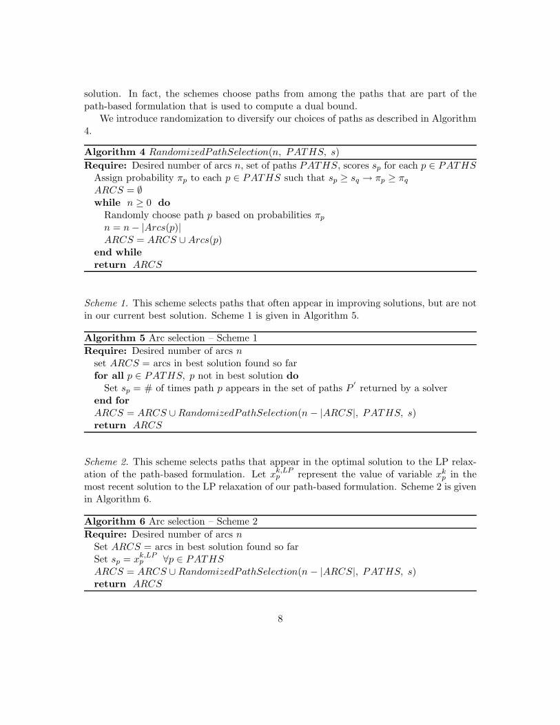
solution. In fact, the schemes choose paths from among the paths that are part of thepath-based formulation that is used to compute a dual bound.
We introduce randomization to diversify our choices of paths as described in Algorithm4.
Algorithm 4 RandomizedPathSelection(n, PATHS, s)
Require: Desired number of arcs n, set of paths PATHS, scores sp for each p ∈ PATHS
Assign probability πp to each p ∈ PATHS such that sp ≥ sq → πp ≥ πq
ARCS = ∅while n ≥ 0 do
Randomly choose path p based on probabilities πp
n = n − |Arcs(p)|ARCS = ARCS ∪ Arcs(p)
end while
return ARCS
Scheme 1. This scheme selects paths that often appear in improving solutions, but are notin our current best solution. Scheme 1 is given in Algorithm 5.
Algorithm 5 Arc selection – Scheme 1
Require: Desired number of arcs n
set ARCS = arcs in best solution found so farfor all p ∈ PATHS, p not in best solution do
Set sp = # of times path p appears in the set of paths P′
returned by a solverend for
ARCS = ARCS ∪ RandomizedPathSelection(n − |ARCS|, PATHS, s)return ARCS
Scheme 2. This scheme selects paths that appear in the optimal solution to the LP relax-ation of the path-based formulation. Let x
k,LPp represent the value of variable xk
p in themost recent solution to the LP relaxation of our path-based formulation. Scheme 2 is givenin Algorithm 6.
Algorithm 6 Arc selection – Scheme 2
Require: Desired number of arcs n
Set ARCS = arcs in best solution found so farSet sp = x
k,LPp ∀p ∈ PATHS
ARCS = ARCS ∪ RandomizedPathSelection(n − |ARCS|, PATHS, s)return ARCS
8

Scheme 3. This scheme selects the path produced for each commodity by the pricingproblem. If these paths do not generate enough arcs, we revert to Scheme 2. Scheme 3 isgiven in Algorithm 7.
Algorithm 7 Arc selection – Scheme 3
Require: Desired number of arcs n
Set ARCS = arcs in best solution found so farSet CG PATHS = ∅for all k do
Solve pricing problem for commodity k
if new path p′
k then
Add p′
k to CG PATHS with score sp′
k
= |cp′
k
|, the absolute value of its reduced cost
end if
end for
ARCS = ARCS ∪ RandomizedPathSelection(n − |ARCS|, CG PATHS, s)if |ARCS| < n then
Set sp = xk,LPp ∀p ∈ PATHS
ARCS = ARCS ∪ RandomizedPathSelection(n − |ARCS|, PATHS, s)end if
4.1.2 Commodity Subset Solves
Given the current solution x and a subset of commodities J , let A′
= {(i, j) ∈ A | xkij =
0 ∀k 6∈ J}, i.e., the set of arcs that is not used by commodities not in J . Let
fij =
{
fij (i, j) ∈ A′
0 (i, j) 6∈ A′
and uij = uij −∑
k 6∈J dkxkij . Then we solve an Arc-FCNF only considering commodities in
J and with fij instead of fij and uij instead of uij . That is, if there exists a commoditynot in J that already uses an arc, we allow the commodities in J to use that arc for free(in terms of the associated fixed cost charge), but we make sure that the available capacityon the arc reflects the flow already on it.
Constructing a feasible solution to the full FCNF instance starting from the solutionto the IP requires updating the paths used by the commodities in J and the appropriateyij variables for (i, j) ∈ A
′
. Note that since we do not have variables yij for (i, j) ∈ A \ A′
our subproblem cannot “turn off” an arc used by a commodity not in J . We can againseed the IP with the paths used by the commodities in J in the current best solution.
Again, we introduce randomization to diversify our choices of commodities as describedin Algorithm 8.
9

Algorithm 8 RandomizedCommoditySelection(n, PATHS, s)
Require: A set of commodities K, set S of scores sk for each commodity k, number n ofcommodities to chooseAssign probability πk to each k ∈ K such that sk ≥ sl → πk ≥ πl
Randomly draw n commodities from K based on probabilities π
Scheme 1. This scheme selects commodities whose paths in the current best solution usearcs (i, j) for which the reduced cost of variable yij, denoted by fij, in the most recentLP solution are far from 0. In an LP solution complementary slackness implies yij = 1only if fij = 0. Thus we re-route commodities away from arcs that are far away from thecomplementary slackness condition. Scheme 1 is given in Algorithm 9.
Algorithm 9 Commodity selection – Scheme 1
Require: Desired number of commodities n
For arc (i, j), let fij be the reduced cost of variable yij in the most recent LP solutionSort arcs in descending order of fij
for all (i, j) in sorted list do
for all k ∈ K do
if commodity k uses arc (i, j) in current best solution then
Select commodity k
if selected n commodities then
breakend if
end if
end for
end for
Scheme 2. Suppose in the current best solution (x, y), there is a node v with three com-modities C1, C2, C3 entering on a single arc, but leaving on three different arcs (see Figure??). When the arcs leaving node v are not fully used, these three commodities are goodcandidates for re-optimization. (Of course, a similar situation occurs when we have mul-tiple commodities entering on different incoming arcs, but leaving on a single outgoingarc.) Assume we have a pre-defined utilization threshold UTIL THRESHOLD, wherewe calculate the utilization of an arc for the current best solution (x, y) as
UTILij =
∑
k∈K dkxkij
uij
.
Then we can score each node based on the number of under-utilized inbound and outboundarcs in the current best solution. Given those scores, we generate probabilities for selecting
10

a node v and hence for selecting a set of commodities. Scheme 2 is given in Algorithm 10.
Algorithm 10 Commodity selection – Scheme 2
for all nodes v do
Set node scorev = 0for all inbound arcs (w, v) do
Calculate UTILw,v
if 0 < UTILw,v < UTIL THRESHOLD then
Set node scorev = node scorev + 1end if
end for
for all outbound arcs (v,w) do
Calculate UTILv,w
if 0 < UTILv,w < UTIL THRESHOLD then
Set node scorev = node scorev + 1end if
end for
end for
Generate node probabilities πv such that node scorev ≥ node scorew → πv ≥ πw
Randomly choose a node v
Choose commodities k such that in solution (x, y),∃w such that xkv,w > 0 or xk
w,v > 0
Scheme 3. Since we want to find sets of commodities that are likely to share arcs, wesearch for commodities whose paths in the current best solution are close together. Givena randomly chosen node v, we perform breadth-first search with v as root. As we discovernodes visited by commodities k in our current best solution, we mark the commodities.Scheme 3 is given in Algorithm 11.
Scheme 4. Suppose the network is very large and there are two commodities k and l thathave only one feasible path from their source to their sink, say pk and pl. In that case, itis unlikely that these paths have a common arc hence re-optimizing commodities k and l
together is not likely to lead to improvements. Conversely, if k and l have many paths, thenthey are likely to share arcs and thus are good candidates to optimize together. During theneighborhood search a collection of feasible paths P (k) is generated for each commodityk. We use these paths in Scheme 4, which is given in Algorithm 12.
Scheme 5. So far the selection schemes have been geared towards improving the currentbest solution. The purpose of this scheme is to provide diversification for our arc subsetsolvers. If there is a commodity k for which we have only generated a single path so far,then an arc subset solver will have little flexibility for re-routing it. Therefore, Scheme 5,
11

Algorithm 11 Commodity selection – Scheme 3
Require: Desired number of commodities n
Set COMMODITIES = ∅Randomly choose a node v
nodes.push(v)while nodes 6= ∅ and |COMMODITIES| < n do
v=nodes.pop()for all k such that xk
w,v > 0 or xkv,w > 0 for some w do
COMMODITIES = COMMODITIES ∪ {k}if |COMMODITIES| = n then
breakend if
end for
for all inbound arcs (w, v) and outbound arcs (v,w) do
nodes.push(w)end for
end while
Algorithm 12 Commodity selection – Scheme 4
Require: Desired number of commodities n
Let P (k) be the set of paths generated for commodity k so farSet sk = |P (k)|return RandomizedCommoditySelection(n, K, s)
given in Algorithm 13, selects commodities for which we have generated very few paths.
Algorithm 13 Commodity selection – Scheme 5
Require: Desired number of commodities n
Let P (k) be the set of paths generated for commodity k so farSet sk = −1 ∗ |P (k)|return RandomizedCommoditySelection(n, K, s)
Scheme 6. The final scheme is specifically designed for instances of FCNF in which acommodity must be routed along a single path. The scheme selects commodities whosedemand is split across many paths in the most recent solution to the LP relaxation of thepath-based formulation. In a sense, we are “repairing” commodities that violate the singlepath constraint in the solution to the LP relaxation of the path-based formulation. Scheme6 is given in Algorithm 14.
12
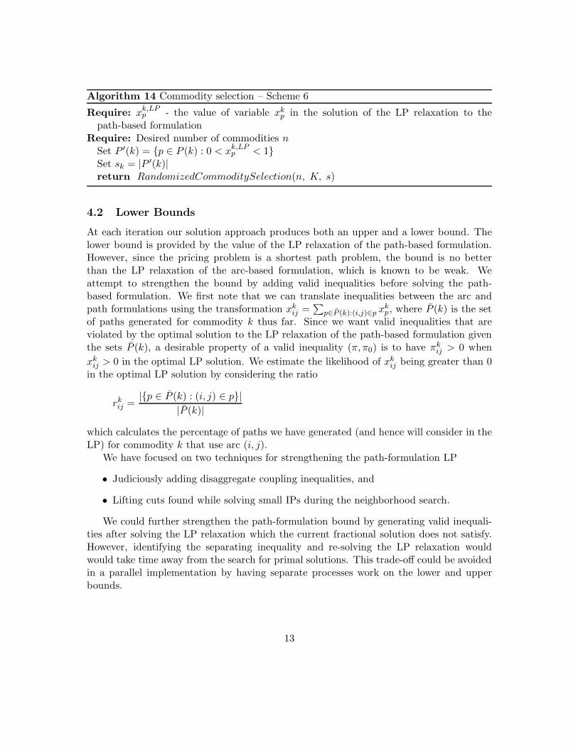
Algorithm 14 Commodity selection – Scheme 6
Require: xk,LPp - the value of variable xk
p in the solution of the LP relaxation to thepath-based formulation
Require: Desired number of commodities n
Set P ′(k) = {p ∈ P (k) : 0 < xk,LPp < 1}
Set sk = |P ′(k)|return RandomizedCommoditySelection(n, K, s)
4.2 Lower Bounds
At each iteration our solution approach produces both an upper and a lower bound. Thelower bound is provided by the value of the LP relaxation of the path-based formulation.However, since the pricing problem is a shortest path problem, the bound is no betterthan the LP relaxation of the arc-based formulation, which is known to be weak. Weattempt to strengthen the bound by adding valid inequalities before solving the path-based formulation. We first note that we can translate inequalities between the arc andpath formulations using the transformation xk
ij =∑
p∈P (k):(i,j)∈p xkp, where P (k) is the set
of paths generated for commodity k thus far. Since we want valid inequalities that areviolated by the optimal solution to the LP relaxation of the path-based formulation giventhe sets P (k), a desirable property of a valid inequality (π, π0) is to have πk
ij > 0 when
xkij > 0 in the optimal LP solution. We estimate the likelihood of xk
ij being greater than 0in the optimal LP solution by considering the ratio
rkij =
|{p ∈ P (k) : (i, j) ∈ p}|
|P (k)|
which calculates the percentage of paths we have generated (and hence will consider in theLP) for commodity k that use arc (i, j).
We have focused on two techniques for strengthening the path-formulation LP
• Judiciously adding disaggregate coupling inequalities, and
• Lifting cuts found while solving small IPs during the neighborhood search.
We could further strengthen the path-formulation bound by generating valid inequali-ties after solving the LP relaxation which the current fractional solution does not satisfy.However, identifying the separating inequality and re-solving the LP relaxation wouldwould take time away from the search for primal solutions. This trade-off could be avoidedin a parallel implementation by having separate processes work on the lower and upperbounds.
13

4.2.1 Disaggregate Inequalities
It is well-known that the disaggregate coupling inequalities (10) strengthen the LP bound,yet due to the great number of them it is typically not possible to add them all. In addition,while adding the disaggregate coupling inequalities strengthens the LP bound they mayalso increase the solve time for the LP relaxation. Of course adding the inequality (10) forcommodity k and arc (i, j) only strengthens the LP bound if in fact
xkij =
∑
p∈P (k):(i,j)∈p
xkp > 0
in the optimal LP solution. Hence we determine the arcs (i, j) and commodities k for whichthe disaggregated coupling constraints will be added using the ratio rk
ij. A threshold valueT ∈ [0, 1] is specified and the inequality is added for commodity k and arc (i, j) only whenrkij ≥ T .
4.2.2 Lifted Cover Inequalities
We have investigated re-using cuts (π, π0) found while solving small IPs during the neigh-borhood search. These cuts are lifted to make them globally valid and to strengthen them.As the inequalities are found while solving small IPs during the neighborhood search, thecomputational effort is only in the lifting process. After lifting, these inequalities are addedto the path formulation to strengthen the bounds its LP relaxation provides.
We have focused our efforts on the single-path variant of FCNF and investigated liftingcover inequalities based on arc capacities. A cover with respect to an arc (i, j) is a setC ⊆ K such that
∑
k∈C dk > uij. Since the variables xkij are binary for the single-path
variant we have the cover inequality∑
k∈C xki,j ≤ |C| − 1.
We use the procedure suggested by Gu et al. (1998) for separating cover inequalities.Note that since the cover inequality is generated during the solution of a commodity subsetIP some variables are fixed to either 0 or 1. As suggested by Gu et al. (1998), we firstuplift variables fixed to 0 and then down-lift those fixed to 1.
It is well known that the strength of the lifted cover inequality depends on the order inwhich the variables fixed to 0 (or 1) are lifted. Therefore we first lift variables xk
ij whosevalue is likely to be positive in the optimal LP solution. Hence, the lifting order is quitesimple: lift in decreasing order of rk
ij . The complete procedure is outlined in Algorithm 15.Currently, we limit ourselves to cover inequalities that are violated in the small IP.
Given that we are especially interested in strengthening the LP relaxation of the path-based formulation, this methodology can be extended to search for cover inequalities thatare not violated in the small IP, but are likely to be violated when all commodities areconsidered.
Since our lifting order depends on the sets P (k) which may change at each iteration, wecould re-lift the cover inequalities as the path sets change and get different valid inequalities.
14

Algorithm 15 Cover Inequality Lifting
Require: Cover Inequality (π, π0) for arc (i, j) from commodity subset IPRequire: Set of commodities K0 such that when generating (π, π0), xk
ij fixed to 0
Require: Set of commodities K1 such that when generating (π, π0), xkij fixed to 1
Calculate rkij = |{p∈P (k):(i,j)⊆p}|
|P (k)|, ∀k ∈ K0 ∪ K1
Uplift variables xkij, k ∈ K0 in descending order of rk
ij
Downlift variables xkij , k ∈ K1 in descending order of rk
ij
return new cut (π′
, π′
0)
However, we do not re-lift because of our time-constrained setting and the computationaleffort lifting requires.
4.3 Initial Feasible Solution
Our scheme for generating an initial feasible solution has two phases. In Phase I we finda path for each commodity by solving a shortest path problem where arc costs reflect alinearized fixed charge and are updated using a slope-scaling approach. Heuristics basedon updating the linearization of the fixed charge are given in Balinski (1961), Crainic et al.(2004), and Kim and Pardalos (1999). The solution to the LP relaxation of Arc-FCNF has
yij = 1uij
∑
k dkxkij, hence we have fijyij =
fij
uij
∑
k dkxkij =
∑
k fijdk
uijxk
ij . This suggests that
we can use a variable cost cij = cijdk + fij
dk
uijfor each arc (i, j) and then solve a shortest
path problem using these arc costs for each commodity k. Instead, we recognize that byassigning paths to commodities sequentially we remove the capacity of some arcs. Hencewe update the variable cost on an arc (i, j) to reflect how much of its capacity remains.The details are given in Algorithm 16.
If we have a feasible solution after Phase I, we stop. Since we do not explicitly enforcethe capacity constraints on arcs during Phase I, we may not end with a feasible solution. Inthis case, we go on to Phase II, where for each arc whose capacity is exceeded, we find a setof commodities to re-route away from the arc in an attempt to “fix the infeasibility.” Thedetails are given in Algorithm 17. Note that this method cannot guarantee that a feasiblesolution is found when one exists, nor can it detect whether an instance is infeasible.
15

Algorithm 16 Phase I algorithm
Sort commodities in descending order of demand dk
Set uij = uij
for k = 1 to K do
Set cij = cij + fij ∗dk
uij
Solve a shortest path problem for commodity k w.r.t. arc costs cij ; let xkij indicate
when arc (i, j) used by k
Set uij = max(1, uij − xkij ∗ dk)
end for
Algorithm 17 Phase II algorithm
while ∃(i, j) :∑
k xkij ∗ dk > uij do
Randomly choose such an (i, j)Sort commodities using the arc (xk
ij = 1) in ascending order of demand dk
Find the smallest l such that∑K
k=l xkij ∗ dk ≤ uij
Solve our commodity subset IP for those first l − 1 commoditiesend while
5 Computational Results
There are many questions to answer regarding the primal and dual-side performance of ourapproach, which we refer to as IP Search. Specifically:
• Primal-Side
– How competitive is IP Search with existing metaheuristics and commercial IPsolvers?
– Is there value in using both commodity subset and arc subset IPs?
– How successful is the method for finding an initial feasible solution?
– Do the solvers contribute equally to finding good solutions?
– Does the biased selection of solvers lead to better solutions?
• Dual-Side
– Does IP Search produce a stronger dual bound than the optimal solution to theLP relaxation of the arc-based formulation?
– Is the dual bound produced by IP Search competitive with the root node boundproduced by a commercial IP solver using an arc-based formulation?
16

– Do the disaggregate inequalities strengthen the dual bound?
– Do the lifted of cover inequalities strengthen the dual bound?
IP Search is implemented in C++ and uses CPLEX 9.1 to solve the subset IPs. Otherthan those taken from the literature, all the results are obtained from experiments per-formed on a machine with 8 Intel Xeon CPUs running at 2.66 GHz and 8 GB RAM.Whenever CPLEX 9.1 is used as a benchmark, it was run with an emphasis on integerfeasibility, with the disaggregate constraints xk
ij ≤ yij added as user cuts, and with anoptimality tolerance set to 5%. All computation times reported are in seconds.
5.1 Instance Generation
A network generator was used to create instances for experimentation. The generatorcreates instances without parallel arcs. The inputs to the generator are:
• The number of nodes, arcs, and commodities in the network
• A range [cl, cu] for arc variable costs
• A range [bl, bu] for commodity quantities
• A range [1, ku] of how many commodities can fit on an arc
• A ratio R of arc fixed cost to variable cost
The generator creates an arc (i, j) by randomly picking nodes i and j. The variable costcij for arc (i, j) is uniformly drawn from [cl, cu]. The fixed cost fij for arc (i, j) is uniformlydrawn from [Rcl, Rcu]. The capacity uij for an arc is set to kb, where k is uniformly drawnfrom [1, ku] and b is uniformly drawn from [bl, bu]. Commodities k are created by randomlypicking pairs of nodes (o(k), d(k)) such that a path exists between the two nodes. Thequantity bk for commodity k is uniformly drawn from [bl, bu]. Finally all commodity andarc data is rounded down to integer values.
We use the same instance classifications as Ghamlouch et al. (2003). An instance isclassified as F if the ratio of fixed to variable cost for an arc is high and V otherwise.An instance is classified as T if the approximate number of commodities that can beaccommodated on an arc is low and L otherwise. Hence we have 4 classes of instances(F, T ), (F,L), (V, T ), (V,L).
5.2 Calibration
Since we solve IPs as subroutines in IP Search, their size is important. If the IP is too largewe may not find a good improving solution in the time alloted to the IP solver. On the otherhand, if the IP is too small it simply may not yield a large enough neighborhood to containa good improving solution. We determine the arc and commodity subset sizes for a specific
17
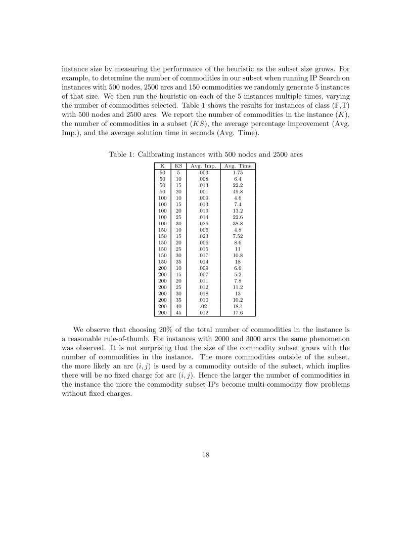
instance size by measuring the performance of the heuristic as the subset size grows. Forexample, to determine the number of commodities in our subset when running IP Search oninstances with 500 nodes, 2500 arcs and 150 commodities we randomly generate 5 instancesof that size. We then run the heuristic on each of the 5 instances multiple times, varyingthe number of commodities selected. Table 1 shows the results for instances of class (F,T)with 500 nodes and 2500 arcs. We report the number of commodities in the instance (K),the number of commodities in a subset (KS), the average percentage improvement (Avg.Imp.), and the average solution time in seconds (Avg. Time).
Table 1: Calibrating instances with 500 nodes and 2500 arcs
K KS Avg. Imp. Avg. Time50 5 .003 1.7550 10 .008 6.450 15 .013 22.250 20 .001 49.8100 10 .009 4.6100 15 .013 7.4100 20 .019 13.2100 25 .014 22.6100 30 .026 38.8150 10 .006 4.8150 15 .023 7.52150 20 .006 8.6150 25 .015 11150 30 .017 10.8150 35 .014 18200 10 .009 6.6200 15 .007 5.2200 20 .011 7.8200 25 .012 11.2200 30 .018 13200 35 .010 10.2200 40 .02 18.4200 45 .012 17.6
We observe that choosing 20% of the total number of commodities in the instance isa reasonable rule-of-thumb. For instances with 2000 and 3000 arcs the same phenomenonwas observed. It is not surprising that the size of the commodity subset grows with thenumber of commodities in the instance. The more commodities outside of the subset,the more likely an arc (i, j) is used by a commodity outside of the subset, which impliesthere will be no fixed charge for arc (i, j). Hence the larger the number of commodities inthe instance the more the commodity subset IPs become multi-commodity flow problemswithout fixed charges.
18

5.3 Upper Bound
5.3.1 Comparison to Tabu Cycle and Path Relink
To examine how IP Search compares with existing metaheuristics, we compared it toa cycle-based tabu-search algorithm (Ghamlouch et al. (2003)) and a cycle-based path-relinking approach (Ghamlouch et al. (2004)) on the instances used in Ghamlouch et al.(2004); except for the 6 instances identified as “easy” (solved in a few seconds by a com-mercial IP solver). Note that the comparison is only for the variant in which commoditiescan be routed along multiple paths (the variant handled by the metaheuristics). The re-sults are shown in Table 2, where we report the instance, the value of the solution foundby CPLEX in 12 hours (CPLEX), the value of the solution obtained by the tabu searchalgorithm (Tabu Cycle), the value of the solution obtained by the path relinking algorithm(Path Relink), the value of the solution obtained by IP Search (IP Search), the percentagedifference between the value of the solution found by IP Search and the value of the solutionfound by CPLEX in 12 hours (CPLEX gap), the percentage difference between the valueof the solution found by IP Search and the best of the values of the solutions found bythe tabu search and path relinking algorithms (Best gap), the optimality gap (Opt gap),and for each of the different algorithms the time to reach the best solution (TTB). Whenwe report a percentage difference (or gap) between IP Search and “X”, it is computed as
100IP Search−XIP Search
. To compute the the optimality gap, we use the dual bound produced by
CPLEX in 12 hours. Note that we imposed a time limit of 15 minutes (900 seconds) on IPSearch.
We first observe that IP Search finds a better solution than the metaheuristics in allbut 2 of the 37 instances. Since different hardware platforms were used to produce themetaheuristic and IP Search results a comparison of computing times cannot be exact.However, the time to the best solution for instance (30,700,400,F,L) indicates that thecomputing time is orders of magnitudes longer for the metaheuristics than for IP Search.For the instance (100,400,10,F,T) the percentage difference between the value of the best ofthe metaheuristics solutions and the value of the solution produced by IP Search is less than1. Hence, we can comfortably conclude that IP Search is superior to these metaheuristics.We next observe that IP Search is producing solutions that are very competitive with thoseproduced by CPLEX in 12 hours. Even though the instances are relatively small, we seethat CPLEX often needs more than 5 hours to find its best solution. Finally, we observethat the optimality gap for the solution produced by IP Search is small, within 5% for 24of the 37 instances and only 3.96% on average.
19

Table 2: Comparison with Tabu Search and Path Relinking
Solution Value TTBCPLEX Tabu Path IP CPLEX Best Opt CPLEX Tabu Path IP
Problem Cycle Relink Search Gap Gap Gap Cycle Relink Search100,400,10,V,L 28,423 28,786 28,485 28,423 0.00 -0.22 0.00 3 252 89 35100,400,10,F,L 23,949 24,022 24,022 23,949 0.00 -0.30 0.00 3,354 196 82 9
100,400,10,F,T 63,764 67,184 65,278 65,885 3.22 0.92 13.97 34,301 451 209 813
100,400,30,V,T 384,802 385,508 384,926 384,836 0.01 -0.02 0.60 1,290 1,199 492 330100,400,30,F,L 49,018 51,831 51,325 49,694 1.36 -3.28 3.44 22,457 717 314 886100,400,30,F,T 138,948 147,193 141,359 141,365 1.71 0.00 11.65 36,001 1,300 480 88820,230,40,V,L 423,848 430,628 424,385 424,385 0.13 0 0.13 1 214 148 420,230,40,V,T 371,475 372,522 371,811 371,779 0.08 -0.01 0.08 1 241 156 4120,230,40,F,T 643,036 652,775 645,548 643,187 0.02 -0.37 0.02 13 259 172 4520,230,200,V,L 94,213 100,001 100,404 95,097 0.93 -5.16 6.21 6,118 2,585 2,494 82220,230,200,F,L 137,642 148,066 147,988 141,253 2.56 -4.77 8.72 8,079 3,142 2,878 69120,230,200,V,T 97,914 106,868 104,689 99,410 1.5 -5.31 4.9 7,097 2,730 2,210 82120,230,200,F,T 132,081 147,212 147,554 140,273 5.84 -4.95 8.06 17,397 3,634 3,386 15620,300,40,V,L 429,398 432,007 429,398 429,398 0 0 0 1 305 224 1920,300,40,F,L 586,077 602,180 590,427 586,077 0 -0.74 0 5 336 228 2920,300,40,V,T 464,509 466,115 464,509 464,509 0 0 0 2 379 247 2420,300,40,F,T 604,198 615,426 609,990 604,198 0 -0.96 0 1 350 214 6820,300,200,V,L 73,335 81,367 78,184 75,319 2.63 -3.8 3.75 36,364 4,086 3,566 80220,300,200,F,L 111,436 122,262 123,484 117,543 5.2 -4.01 7.18 42,220 4,210 4,012 68620,300,200,V,T 74,991 80,344 78,866 76,198 1.58 -3.5 3.44 6,490 4,204 3,924 38820,300,200,F,T 103,967 113,947 113,584 110,344 5.78 -2.94 7.08 42,585 4,855 3,857 39630,520,100,V,L 53,958 56,603 54,904 54,113 0.29 -1.46 0.82 436 2,261 1,194 21830,520,100,F,L 90,488 103,657 102,054 94,388 4.13 -8.12 7.78 39,409 2,684 1,459 22630,520,100,V,T 51,475 54,454 53,017 52,174 1.34 -1.62 1.34 38,260 2,716 1,513 45530,520,100,F,T 94,199 105,130 106,130 98,883 4.74 -6.32 5.97 39,302 2,892 1,522 81530,520,400,V,L 111,844 122,673 119,416 114,042 1.93 -4.71 2.85 36,436 55,771 27,477 39430,520,400,F,L 145,430 164,140 163,112 154,218 5.7 -5.77 5.79 30,624 40,070 36,669 75030,520,400,V,T 114,133 122,655 120,170 114,922 0.69 -4.57 0.97 31,588 4,678 23,089 62130,520,400,F,T 149,009 169,508 163,675 154,606 3.62 -5.87 3.72 31,127 49,886 52,173 46630,700,100,V,L 47,603 50,041 48,723 47,612 0.02 -2.33 0.02 205 2,959 1,860 3230,700,100,F,L 58,767 64,581 63,091 60,700 3.18 -3.94 6.22 18,900 3,182 1,837 74130,700,100,V,T 45,199 48,176 47,209 46,046 1.84 -2.53 2.21 34,111 3,746 1,894 37130,700,100,F,T 53,815 57,628 56,575 55,609 3.23 -1.74 4.78 39,396 3,547 1,706 38730,700,400,V,L 96,063 107,727 105,116 98,718 2.69 -6.48 2.93 40,901 38,857 22,314 222
30,700,400,F,L 129,094 150,256 145,026 152,576 15.39 4.95 15.42 10,231 68,214 75,664 860
30,700,400,V,T 93,626 101,749 101,212 96,168 2.64 -5.24 2.81 37,661 51,764 24,288 36530,700,400,F,T 126,779 144,852 141,013 131,629 3.68 -7.13 3.79 5,464 79,053 44,936 225
Average 2.37 -2.76 3.96 18860.30 12106.08 9431.81 408.14
20

Table 3: Primal-side Comparison with CPLEXCPLEX-15M CPLEX-12H IP Search CPLEX-15M CPLEX-12H Opt
Problem Gap Gap Gap500,2000,50,F,L 5,301,081 5,301,081 3,910,120 -35.57 -35.57 55.94500,2000,50,F,T X 7,927,065 5,249,040 N/A -51.02 31.14500,2000,100,F,L 8,944,724 8,299,799 6,764,310 -32.23 -22.70 63.52500,2000,100,F,T 10,199,000 8,306,181 7,718,750 -32.13 -7.61 31.84500,2000,150,F,L 10,996,000 10,080,000 8,618,060 -27.59 -16.96 63.78500,2000,150,F,T 12,115,000 10,770,000 9,448,890 -28.22 -13.98 65.32500,2000,200,F,L 13,808,000 12,824,000 10,333,200 -33.63 -24.10 64.37500,2000,200,F,T X X 12,425,600 N/A N/A 49.63500,2500,50,F,L 4,611,275 4,611,275 3,841,350 -20.04 -20.04 70.88500,2500,50,F,T 5,779,926 5,084,529 4,666,740 -23.85 -8.95 32.56500,2500,100,F,L 9,351,042 9,251,042 6,875,420 -36.01 -34.55 71.97500,2500,100,F,T 9,724,997 7,995,284 7,235,520 -34.41 -10.50 46.31500,2500,150,F,L 13,660,000 12,497,000 9,730,100 -40.39 -28.44 77.45500,2500,150,F,T 11,385,000 10,683,000 7,934,360 -43.49 -34.64 72.22500,2500,200,F,L 15,539,000 13,468,000 11,261,300 -37.99 -19.60 75.02500,2500,200,F,T 18,906,000 14,948,000 12,825,300 -47.41 -16.55 58.30500,3000,50,F,L 5,098,318 5,098,318 3,596,980 -41.74 -41.74 76.27500,3000,50,F,T 5,615,096 4,866,768 4,504,260 -24.66 -8.05 41.85500,3000,100,F,L 8,721,798 8,721,798 6,577,980 -32.59 -32.59 75.06500,3000,100,F,T 10,119,000 8,330,109 7,517,970 -34.60 -10.80 49.67500,3000,150,F,L 12,628,000 12,623,000 9,214,960 -37.04 -36.98 80.31500,3000,150,F,T 12,615,000 10,147,000 9,186,840 -37.32 -10.45 55.71500,3000,200,F,L 15,039,000 13,441,000 10,853,400 -38.56 -23.84 80.03500,3000,200,F,T 17,883,000 13,674,000 11,578,000 -54.46 -18.10 58.35
Average -35.18 -22.95 60.31
5.3.2 Comparison to Commercial IP Solver
Next we focus on the performance of IP Search on large instances for the variant in whicheach commodity has to be routed along a single path by comparing the value of the solutionproduced to the value of the solution produced by CPLEX in 15 minutes (CPLEX-15M)and in 12 hours (CPLEX-12H). We consider 24 instances of the classes (F,T) and (F,L),which we refer to as the GT instances. The results are given in Table 3. An “X” in acolumn indicates that no feasible solution was found. As before, the value reported for IPSearch is the value of the solution produced within 15 minutes.
We observe that in every instance IP Search finds a better solution in 15 minutes thanCPLEX does in 12 hours. We also see that the improvement over the solution foundby CPLEX in 15 minutes is significant, often greater than 30%. Even the improvementover the solution found by CPLEX in 12 hours is impressive, often greater than 20%.Unfortunately, little can be said with confidence regarding the true optimality gap of thesolutions produced by IP Search since the dual bounds produced by CPLEX change verylittle over the course of the execution and are likely to be weak. In fact, for many of theloosely capacitated instances, CPLEX did not find a significantly better primal solution in12 hours than it did in 15 minutes. This highlights the difficulty that an LP-based branch-and-bound algorithm can have in finding good primal solutions when the dual bounds are
21

weak.In Table 4 we see that IP Search not only outperforms CPLEX, but it does so in very
little time, needing on average less than 3 minutes to produce a solution that is better thanthe best solution produced by CPLEX in 12 hours. The time limit of 15 minutes on IP
Table 4: Heuristic Time To Beat CPLEXCPLEX CPLEX
Problem 15 M Primal 12 H Primal500,2000,50,F,L 10 10500,2000,50,F,T 16 16500,2000,100,F,L 98 98500,2000,100,F,T 49 343500,2000,150,F,L 46 119500,2000,150,F,T 45 294500,2000,200,F,L 44 280500,2000,200,F,T 19 19500,2500,50,F,L 82 82500,2500,50,F,T 10 23500,2500,100,F,L 32 32500,2500,100,F,T 77 226500,2500,150,F,L 24 47500,2500,150,F,T 50 115500,2500,200,F,L 57 289500,2500,200,F,T 37 142500,3000,50,F,L 17 17500,3000,50,F,T 5 296500,3000,100,F,L 27 27500,3000,100,F,T 120 365500,3000,150,F,L 22 22500,3000,150,F,T 30 338500,3000,200,F,L 50 75500,3000,200,F,T 10 104
Average 41 141
Search is, of course, self-imposed. Table 5 reports the results for IP Search after 15, 30, and60 minutes as well as the percentage improvement over the initial solution found. We seethat the greatest percentage improvement occurs in the first 15 minutes, but that IP Searchcontinues to find improving solutions when given more time. The column labeled “TimesPhase II” gives the number of times Phase II of the scheme for finding an initial feasiblesolution is executed. Not surprisingly, Phase II is only executed for tightly-capacitatedinstances. In fact, for the majority of instances Phase II is not needed at all.
22

Table 5: IP Search Given More TimeTimes Init. Feas. 15 Minute 30 Minute 60 Minute Imp. After Imp. After Imp. After
Problem Phase II Soln Soln Soln Soln 15 M 30 M 60M500,2000,50,F,L 0 6,175,840 3,910,120 3,907,440 3,823,610 -36.69 -36.73 -38.09500,2000,50,F,T 5 6,314,980 5,249,040 5,112,490 4,949,780 -16.88 -19.04 -21.62500,2000,100,F,L 0 10,244,000 6,764,310 6,655,370 6,453,880 -33.97 -35.03 -37.00500,2000,100,F,T 4 10,125,700 7,718,750 7,632,220 7,619,670 -23.77 -24.63 -24.75500,2000,150,F,L 0 13,317,800 8,618,060 8,279,270 8,081,600 -35.29 -37.83 -39.32500,2000,150,F,T 0 14,557,800 9,448,890 9,250,760 8,807,650 -35.09 -36.45 -39.50500,2000,200,F,L 0 17,411,800 10,333,200 10,138,900 9,828,350 -40.65 -41.77 -43.55500,2000,200,F,T 0 17,543,000 12,425,600 12,117,800 11,893,100 -29.17 -30.93 -32.21500,2500,50,F,L 0 5,712,380 3,841,350 3,780,160 3,612,030 -32.75 -33.83 -36.77500,2500,50,F,T 1 5,898,160 4,666,740 4,661,160 4,600,200 -20.88 -20.97 -22.01500,2500,100,F,L 0 10,640,700 6,875,420 6,621,140 6,400,140 -35.39 -37.78 -39.85500,2500,100,F,T 1 10,077,400 7,235,520 7,065,020 6,953,660 -28.20 -29.89 -31.00500,2500,150,F,L 0 14,834,200 9,730,100 9,475,760 9,089,920 -34.41 -36.12 -38.72500,2500,150,F,T 0 13,365,000 7,934,360 7,673,410 7,571,640 -40.63 -42.59 -43.35500,2500,200,F,L 0 17,446,900 11,261,300 10,623,700 10,099,200 -35.45 -39.11 -42.11500,2500,200,F,T 1 18,628,100 12,825,300 11,843,200 11,452,900 -31.15 -36.42 -38.52500,3000,50,F,L 0 5,687,990 3,596,980 3,519,400 3,457,280 -36.76 -38.13 -39.22500,3000,50,F,T 0 5,553,000 4,504,260 4,405,120 4,262,350 -18.89 -20.67 -23.24500,3000,100,F,L 0 10,383,600 6,577,980 6,202,380 6,015,950 -36.65 -40.27 -42.06500,3000,100,F,T 2 10,350,000 7,517,970 7,444,950 7,186,810 -27.36 -28.07 -30.56500,3000,150,F,L 0 13,707,300 9,214,960 9,126,970 8,919,720 -32.77 -33.42 -34.93500,3000,150,F,T 0 12,958,300 9,186,840 8,898,880 8,709,390 -29.10 -31.33 -32.79500,3000,200,F,L 0 16,869,900 10,853,400 10,419,400 10,040,000 -35.66 -38.24 -40.49500,3000,200,F,T 1 17,071,600 11,578,000 10,750,200 10,390,700 -32.18 -37.03 -39.13
Average -31.66 -33.59 -35.45
We observed in Table 3 that IP Search significantly outperforms CPLEX on largeinstances when each commodity has to be routed along a single path. Next we investigatewhat happens when we have small instances but require a commodity to be routed along asingle path. The results are given in Table 6. As before, IP Search is limited to 15 minutes.When CPLEX obtains a better solution than IP Search, we report how long it took CPLEXto find the first solution that is better than the solution found by IP Search (CPLEX TimeBeat). We observe that in only 2 of the 37 instances does CPLEX find a better solution in15 minutes than IP Search. In those 2 instances the difference in solution value between IPSearch and CPLEX is less than .15%. On the other hand, IP Search often finds solutionsthat are 5% better than what CPLEX finds in 15 minutes. The optimality gap informationreveals that the solutions produced by IP Search are of high quality, on average within4% of optimality. When CPLEX does find a better solution, it often requires more than 3hours to do so. We also see that IP Search produces solutions within 15 minutes that arecompetitive with what CPLEX produces in 12 hours. CPLEX’s best improvement overIP Search occurs for instance (100,400,30,F,L) where it finds a solution that is only 4.52%better than IP Search.
23

Table 6: Primal-side Comparison with CPLEX - Metaheuristic Instances - Single Path
ProblemCPLEX-15M CPLEX-12H IP Search CPLEX-15M CPLEX-12H Opt CPLEX
Gap Gap Gap Time Beat100,400,10,V,L 31,785 31,785 31,785 0 0 0 -100,400,10,F,L 24,104 24,104 24,104 0 0 0 -100,400,10,F,T 328,177 328,177 328,177 0 0 0 -100,400,30,V,T 750,420 750,420 750,420 0 0 0 -100,400,30,F,L 55,665 50,391 52,779 -5.47 4.52 6.90 10,998100,400,30,F,T 188,113 188,113 188,113 0 0 0 -20,230,40,V,L 423,933 423,933 424,671 0.17 0.17 0.17 120,230,40,V,T 398,870 398,870 398,870 0 0 0 -20,230,40,F,T 668,699 668,699 668,699 0 0 0 -20,230,200,V,L 102,118 95,126 96,456 -5.87 1.38 5.18 2,59520,230,200,F,L 160,535 141,197 141,700 -13.29 0.35 6.37 -20,230,200,V,T 107,145 100910 100,884 -6.21 -0.03 6.4 24,46920,230,200,F,T 157,874 143781 141,734 -11.39 -1.44 8.98 -20,300,40,V,L 430,253 430,253 430,253 0 0 0 -20,300,40,F,L 597,059 597,059 597,059 0 0 0 -20,300,40,V,T 501,766 501,766 501,766 0 0 0 -20,300,40,F,T 643,395 643,395 643,395 0 0 0 -20,300,200,V,L 81,101 78262 76,946 -5.4 -1.71 5.7 -20,300,200,F,L 128,871 120301 119,590 -7.76 -0.59 8.14 -20,300,200,V,T 78,900 77303 77,858 -1.34 0.71 4.99 17,40320,300,200,F,T 120,997 110897 110,609 -9.39 -0.26 6.1 20,91130,520,100,V,L 54,394 54,387 54,454 0.11 0.12 0.12 30830,520,100,F,L 103,771 98797 97,199 -6.76 -1.64 6.34 -30,520,100,V,T 53,812 53,812 53,812 0 0 0 -30,520,100,F,T 102,186 99204 100,871 -1.3 1.65 4.35 8,67730,520,400,V,L 132,799 120781 117,078 -13.43 -3.16 5.25 -30,520,400,F,L 164,469 159146 157,682 -4.3 -0.93 7.92 -30,520,400,V,T 132,935 120326 118,214 -12.45 -1.79 3.63 -30,520,400,F,T 166,561 158396 161,577 -3.08 1.97 7.87 22,89730,700,100,V,L 47,883 47,883 47,883 0 0 0 -30,700,100,F,L 63,275 60856 61,254 -3.3 0.65 3.43 12,10930,700,100,V,T 47,864 47,670 47,736 -0.27 0.14 0.14 1,23630,700,100,F,T 57,218 56686 57,125 -0.16 0.77 0.77 2,01930,700,400,V,L 103,839 100332 102,216 -1.59 1.84 6.28 12,59930,700,400,F,L 677,227 151043 144,077 -370.05 -4.83 10.48 -30,700,400,V,T 100,937 99972 99,118 -1.84 -0.86 5.52 -30,700,400,F,T 142,604 137149 138,787 -2.75 1.18 8.68 11,605
Average -13.17 -0.05 3.51 10,559.07
5.3.3 Value of Subset Solvers
Table 7 shows the performance of standard IP Search, IP Search using only arc subsetIPs, and IP Search using only commodity subset IPs. The percentage difference, or gap,
information for only using subset type X is calculated as 100X−Arc & Commodity
Arc & Commodity. We
observe that using each subset IP type by itself is already effective, sometimes even moreeffective than using them in combination, but that on average the combination yields bettersolutions.
24

Table 7: Value of subset IP typesArc + Commodity Arc Arc Commodity Commodity
Problem Gap Gap500,2000,50,F,L 3,910,120 4,256,180 8.85 4,066,470 4.00500,2000,50,F,T 5,249,040 5,682,850 8.26 5,330,480 1.55500,2000,100,F,L 6,764,310 7,425,740 9.78 6,735,860 -0.42500,2000,100,F,T 7,718,750 8,549,650 10.76 8,089,280 4.80500,2000,150,F,L 8,618,060 8,988,500 4.30 9,207,030 6.83500,2000,150,F,T 9,448,890 9,257,380 -2.03 9,587,780 1.47500,2000,200,F,L 10,333,200 10,880,100 5.29 11,229,800 8.68500,2000,200,F,T 12,425,600 13,030,400 4.87 12,581,300 1.25500,2500,50,F,L 3,841,350 4,286,400 11.59 3,960,530 3.10500,2500,50,F,T 4,666,740 4,939,120 5.84 4,635,180 -0.68500,2500,100,F,L 6,875,420 7,136,500 3.80 6,909,580 0.50500,2500,100,F,T 7,235,520 7,796,070 7.75 7,859,290 8.62500,2500,150,F,L 9,730,100 10,013,900 2.92 9,570,420 -1.64500,2500,150,F,T 7,934,360 8,604,130 8.44 8,497,240 7.09500,2500,200,F,L 11,261,300 11,188,600 -0.65 11,714,800 4.03500,2500,200,F,T 12,825,300 12,816,900 -0.07 12,947,200 0.95500,3000,50,F,L 3,596,980 4,390,700 22.07 3,759,470 4.52500,3000,50,F,T 4,504,260 4,855,100 7.79 4,380,330 -2.75500,3000,100,F,L 6,577,980 7,366,460 11.99 6,468,730 -1.66500,3000,100,F,T 7,517,970 8,211,270 9.22 8,303,140 10.44500,3000,150,F,L 9,214,960 10,222,900 10.94 9,479,810 2.87500,3000,150,F,T 9,186,840 9,204,010 0.19 9,206,770 0.22500,3000,200,F,L 10,853,400 11,495,100 5.91 11,013,700 1.48500,3000,200,F,T 11,578,000 11,838,700 2.25 11,606,100 0.24
Average 6.67 2.73
To gain a greater understanding of the efficacy of each selection scheme, we examine indetail the contribution of each on finding improving solutions. Table 8 gives the breakdownby scheme, averaged over the GT instances, after running IP Search for 60 minutes. Wereport the percentage of iterations a scheme was executed (% Called) and the percentageimprovement that can be attributed to a scheme (% Improvement). The schemes are de-noted by A-x for arc subset selection scheme x and C-x for commodity subset selectionscheme x. We observe that the vast majority of solution improvement is due to the com-
Table 8: Selection Method ContributionScheme % Called % Total Improvement
A-1 6 3A-2 4 2A-3 9 8C-1 14 13C-2 10 4C-3 13 9C-4 14 16C-5 14 28C-6 16 17
modity subset IPs. This may simply be due to the biased random selection mechanismrepeatedly selecting the commodity subset solvers because of their effectiveness. Commod-
25

ity selection scheme 5 results in the largest percentage improvement. Recall that this isthe scheme that selects commodities for which few paths have been discovered and was de-signed to aid in diversification for the arc subset solvers. These results indicate the schemeis effective in finding improving solutions itself.
We also see that the biased randomized selection appears to be working properly asthe most effective selection methods are called most frequently. To further evaluate thevalue of the biased random selection, we compare it to a simple round-robin approachfor selecting solvers. Our simple round-robin scheme executes the solvers in the follow-ing order: A-1, C-1, C-2, A-2, C-3, C-4, A-3, C-5, and C-6. The results are given inTable 9 where we report the value of the solution obtained when using the biased ran-dom selection (Biased Random), the value of the solution obtained when using simpleround-robin (Round Robin), and the percentage difference between the two, calculated as
100Round Robin−Biased RandomRound Robin
. We see that biased random selection does better thanround-robin, but not significantly better. Of course, it may be that we have simply chosenan effective order for the round-robin scheme. The results indicate that IP Search is robustin the sense that the choice of subset type and the choice of subset selection scheme has arelatively minor impact on the overall effectiveness.
Table 9: Biased Random vs. Round RobinProblem Biased Random Round Robin Gap
500,2000,50,F,L 3,910,120 4,029,970 3.07500,2000,50,F,T 5,249,040 5,260,950 0.23500,2000,100,F,L 6,764,310 6,732,430 -0.47500,2000,100,F,T 7,718,750 7,944,700 2.93500,2000,150,F,L 8,618,060 9,134,460 5.99500,2000,150,F,T 9,448,890 8,996,460 -4.79500,2000,200,F,L 10,333,200 10,615,300 2.73500,2000,200,F,T 12,425,600 12,447,300 0.17500,2500,50,F,L 3,841,350 3,862,160 0.54500,2500,50,F,T 4,666,740 4,701,030 0.73500,2500,100,F,L 6,875,420 7,014,860 2.03500,2500,100,F,T 7,235,520 7,254,500 0.26500,2500,150,F,L 9,730,100 9,817,410 0.90500,2500,150,F,T 7,934,360 8,770,120 10.53500,2500,200,F,L 11,261,300 10,898,400 -3.22500,2500,200,F,T 12,825,300 13,167,700 2.67500,3000,50,F,L 3,596,980 3,681,570 2.35500,3000,50,F,T 4,504,260 4,545,940 0.93500,3000,100,F,L 6,577,980 6,520,750 -0.87500,3000,100,F,T 7,517,970 8,389,710 11.60500,3000,150,F,L 9,214,960 9,675,770 5.00500,3000,150,F,T 9,186,840 9,522,640 3.66500,3000,200,F,L 10,853,400 11,729,700 8.07500,3000,200,F,T 11,578,000 12,053,100 4.10
Average 2.46
26

5.4 Lower Bound
We have conducted some computational experiments to analyze the quality of the lowerbounds produced. Since we want to evaluate the value of the lifted cover inequalities, weonly consider the single-path variant of FCNF. First we compare the lower bound IP Searchproduces with the value of the LP relaxation of the arc-based formulation and with theroot node bound CPLEX produces. Since the disaggregate coupling constraints are addedas user cuts, they are not present in the LP relaxation, but are reflected in the root nodebound in addition to any other cuts generated by CPLEX.
The results are shown in Table 10, where we report the value of the LP-relaxation(LPR), the value of the root node bound (Root Node), the lower bound IP Search pro-duces, and the percentage differences between the bound IP Search produces and theother two bounds (LP Gap and Root Gap). The percentage differences are calculated as
100IP Search−LPRIP Search
and 100Root Node−IP SearchRoot Node
. Note that this means a positive per-centage difference with the value of the LP Relaxation indicates that IP Search has given astronger lower bound and a positive percentage difference with the value of the root nodeLP indicates that CPLEX has a stronger root node bound. We observe that IP Search
Table 10: Dual-side Comparison with CPLEX - GT Instances
ProblemLPR Root IP Search LP Root
Node Gap Gap500,2000,50,F,L 749,167 1,722,684 1,205,430 37.85 30.03500,2000,50,F,T 2,289,020 3,614,601 2,717,780 15.78 24.81500,2000,100,F,L 1,069,554 2,466,756 1,803,010 40.68 26.91500,2000,100,F,T 3,401,818 5,257,456 3,687,050 7.74 29.87500,2000,150,F,L 1,629,223 3,121,039 2,537,120 35.78 18.71500,2000,150,F,T 1,761,529 3,276,022 2,792,120 36.91 14.77500,2000,200,F,L 2,051,456 3,679,590 3,230,900 36.51 12.19500,2000,200,F,T 4,198,214 6,259,068 5,464,430 23.17 12.70500,2500,50,F,L 554,544 1,118,701 757,794 26.82 32.26500,2500,50,F,T 1,970,332 3,144,840 2,162,030 8.87 31.25500,2500,100,F,L 801,012 1,927,414 1,301,380 38.45 32.48500,2500,100,F,T 2,325,097 3,884,996 2,747,240 15.37 29.29500,2500,150,F,L 1,122,028 2,194,102 1,682,550 33.31 23.31500,2500,150,F,T 1,119,283 2,192,494 1,721,910 35.00 21.46500,2500,200,F,L 1,663,847 2,811,792 2,752,630 39.55 2.10500,2500,200,F,T 3,576,177 5,347,065 4,397,850 18.68 17.75500,3000,50,F,L 447,750 853,592 600,636 25.45 29.63500,3000,50,F,T 1,629,701 2,618,366 1,755,360 7.16 32.96500,3000,100,F,L 886,097 1,640,026 1,164,540 23.91 28.99500,3000,100,F,T 2,222,056 3,783,508 2,499,770 11.11 33.93500,3000,150,F,L 1,017,504 1,813,662 1,424,980 28.60 21.43500,3000,150,F,T 2,551,015 4,068,577 2,992,860 14.76 26.44500,3000,200,F,L 1,236,509 2,165,713 1,791,940 31.00 17.26500,3000,200,F,T 3,299,636 4,822,044 3,819,270 13.61 20.80
Average 25.25 23.81
produces lower bounds which are much stronger than the value of the LP Relaxation. Fur-thermore, the difference is larger for loosely capacitated instances. On the other hand we
27

see that CPLEX produces a much stronger bound at the root node.Next, we perform the same comparison for the Ghamlouch instances. The results are
shown in Table 11. We observe that for these small instances, IP Search produces weakerlower bounds, often less than the value of the LP relaxation. The average values arestrongly influenced by two instances, (100,400,10,F,T) and (100,400,30,V,T). When weignore these instances, IP Search produces better bounds. At the same time, the differencebetween the lower bound of IP Search and the root node bound CPLEX produces has alsonarrowed.
Table 11: Dual-side Comparison with CPLEX - Metaheuristic Instances
ProblemLPR Root IP Search LP Root
Node Gap Gap100,400,10,V,L 31,167 31,785 27,343 -13.99 -16.25100,400,10,F,L 11,719 22,197 12,342 5.05 -79.85100,400,10,F,T 289,118 328,177 41,520 -596.33 -690.41100,400,30,V,T 711,036 750,420 378,722 -87.75 -98.15100,400,30,F,L 23,498 41,336 30,731 23.54 -34.51100,400,30,F,T 148,330 188,113 106,334 -39.49 -76.9120,230,40,V,L 378,623 422,778 363,348 -4.2 14.0620,230,40,V,T 376,393 398,820 398,870 5.64 -0.0120,230,40,F,T 609,411 668,699 618,803 1.52 7.4620,230,200,V,L 68,805 88,873 71,296 3.49 19.7820,230,200,F,L 98,342 128,039 102,808 4.34 19.7120,230,200,V,T 73,975 94,211 78,952 6.3 16.220,230,200,F,T 100,728 128,768 100,370 -0.36 22.0520,300,40,V,L 386,461 430,253 376,500 -2.65 12.4920,300,40,F,L 492,690 583,079 553,120 10.93 5.1420,300,40,V,T 473,755 501,233 394,472 -20.1 21.320,300,40,F,T 572,481 643,395 563,965 -1.51 12.3520,300,200,V,L 58,934 72,358 59,772 1.4 17.3920,300,200,F,L 87,877 109,033 86,353 -1.76 20.820,300,200,V,T 61,481 73,427 64,765 5.07 11.820,300,200,F,T 84,733 102,436 88,939 4.73 13.1830,520,100,V,L 44,118 53,010 48,606 9.23 8.3130,520,100,F,L 67,559 87,169 68,312 1.1 21.6330,520,100,V,T 47,429 52,897 48,957 3.12 7.4530,520,100,F,T 76,709 93,569 77,083 0.49 17.6230,520,400,V,L 96,690 110,937 100,603 3.89 9.3230,520,400,F,L 122,679 145,201 125,903 2.56 13.2930,520,400,V,T 100,648 113,928 104,874 4.03 7.9530,520,400,F,T 126,356 148,830 127,283 0.73 14.4830,700,100,V,L 39,055 47,061 43,468 10.15 7.6330,700,100,F,L 45,708 57,121 47,836 4.45 16.2530,700,100,V,T 41,798 46,561 42,788 2.31 8.130,700,100,F,T 45,026 54,228 48,330 6.84 10.8830,700,400,V,L 79,059 95,744 82,330 3.97 14.0130,700,400,F,L 106,564 128,969 108,054 1.38 16.2230,700,400,V,T 81,216 93,593 85,416 4.92 8.7430,700,400,F,T 109,364 126,739 110,959 1.44 12.45
Average -17.18 -15.89
Since both disaggregate coupling constraints and lifted cover inequalities are used to
28

strengthen the dual bound IP Search produces, we next analyze their respective contribu-tions. Table 12 shows the value of the LP relaxation (LPR), the value of the LP relaxationwith judiciously added disaggregated coupling constraints (LPR + disaggr), and the valueof the LP relaxation with judiciously added disaggregated coupling constraints and liftedcover inequalities (LPR + disaggr + cover). We observe that the judiciously selected dis-aggregate coupling constraint contribute the most to the bound improvement. We alsoobserve that with a threshold value T = .25 we typically only add 1% of the possibledisaggregate coupling constraints. Not surprisingly, the lifted cover inequalities are mosteffective for tightly-capacitated instances.
Table 12: Disaggregate vs. Cover Inequalities
ProblemLPR Only Imp. Disagg Imp. .
Disagg Gap & Cover Gap500,2000,50,F,L 749,167 1,113,400 32.71 1,205,430 37.85500,2000,50,F,T 2,289,020 2,617,900 12.56 2,717,780 15.78500,2000,100,F,L 1,069,554 1,699,710 37.07 1,803,010 40.68500,2000,100,F,T 3,401,818 3,518,480 3.32 3,687,050 7.74500,2000,150,F,L 1,629,223 2,446,600 33.41 2,537,120 35.78500,2000,150,F,T 1,761,529 2,524,590 30.23 2,792,120 36.91500,2000,200,F,L 2,051,456 3,129,100 34.44 3,230,900 36.51500,2000,200,F,T 4,198,214 5,335,330 21.31 5,464,430 23.17500,2500,50,F,L 554,544 698,710 20.63 757,794 26.82500,2500,50,F,T 1,970,332 2,098,610 6.11 2,162,030 8.87500,2500,100,F,L 1,069,554 1,272,720 15.96 1,301,380 17.81500,2500,100,F,T 2,325,097 2,700,930 13.91 2,747,240 15.37500,2500,150,F,L 1,122,028 1,626,530 31.02 1,682,550 33.31500,2500,150,F,T 1,119,283 1,642,180 31.84 1,721,910 35500,2500,200,F,L 1,663,847 2,607,580 36.19 2,752,630 39.55500,2500,200,F,T 3,576,177 4,294,910 16.73 4,397,850 18.68500,3000,50,F,L 447,750 597,728 25.09 600,636 25.45500,3000,50,F,T 1,629,701 1,674,410 2.67 1,755,360 7.16500,3000,100,F,L 886,097 1,163,210 23.82 1,164,540 23.91500,3000,100,F,T 2,222,056 2,430,220 8.57 2,499,770 11.11500,3000,150,F,L 1,017,504 1,252,230 18.74 1,424,980 28.6500,3000,150,F,T 2,551,015 2,894,492 11.87 2,992,860 14.76500,3000,200,F,L 1,236,509 1,780,330 30.55 1,791,940 31500,3000,200,F,T 3,299,636 3,720,500 11.31 3,819,270 13.61
Average 21.25 24.39
6 Conclusions
We have proposed a local search heuristic (IP Search) for the fixed charge network flowproblem capable of producing high-quality feasible solutions, as well as lower bounds, ina short amount of time. Unlike traditional local search heuristics, we rely on exponential-sized neighborhoods which we search using integer programming technology. Since we useinteger programming technology to search neighborhoods, the heuristic can easily handlethe different variants of the problem, e.g., with arc capacities, without arc capacities,
29

commodities have to be routed along a single path, commodities can be routed alongmultiple paths, etc.
Computational experiments demonstrate that IP Search is superior to existing meta-heuristics and pure integer programming approaches when it comes to producing high-quality primal solutions quickly. Since IP Search produces a lower bound by strengtheningthe LP relaxation with a limited set of valid inequalities, the bound produced (like thoseproduced by pure integer programming solves) is relatively weak.
IP Search can easily be parallelized, which will likely allow it to produce high-qualitysolutions even faster. This is at the top of our list for future research. IP Search makesextensive use of both the compact (arc-based) and extended (path-based) formulation ofFCNF and we believe this is one reason for its success. Therefore we plan to investigatewhether the general framework of IP Search will be successful on other hard discreteoptimization problems.
References
Ahuja, R., Ergun, O., Orlin, J., and Punnen, A. (2002). A survery of very large scaleneighborhood search techniques. Discrete Applied Mathematics, 123:75–102.
Archetti, C., Speranza, M. G., and Savelsbergh, M. W. P. (2008). An optimization-basedheuristic for the split delivery vehicle routing problem. Transportation Science, 42:22–31.
Balinski, M. (1961). Fixed cost transportation problem. Nav. Res. Logistics Q., 8:41–54.
Crainic, T., Frangioni, A., and Gendron, B. (2001). Bundle-based relaxation methods formulticommodity capacitated fixed charge network design. Discrete Applied Mathematics,112:73–99.
Crainic, T. and Gendreau, M. (2002). Cooperative parallel tabu search for capacitatednetwork design. Journal of Heuristics, 8:601–627.
Crainic, T., Gendreau, M., and Farvolden, J. (2000). A simplex-based tabu search methodfor capacitated network design. INFORMS J. Comput., 12:223–236.
Crainic, T., Gendron, B., and Hernu, G. (2004). A slope scaling/lagrangean perturbationheuristic with long-term memory for multicommodity capacitated fixed-charge networkdesign. Journal of Heuristics, 10:525–545.
Danna, E., Rothberg, E., and Le Pape, C. (2005). Exploring relaxation induced neighbor-hoods to improve MIP solutions. Mathematical Programming, 102:71–90.
De Franceschi, R., Fischetti, M., and Toth, P. (2006). A new ILP-based refinement heuristicfor vehicle routing problems. Mathematical Programming B, 105:471–499.
30

Fischetti, M. and Lodi, A. (2003). Local branching. Mathematical Programming, 98:23–47.
Ghamlouch, I., Crainic, T., and Gendreau, M. (2003). Cycle-based neighborhoods for fixedcharge capacitated multicommodity network design. Operations Research, 51:655–667.
Ghamlouch, I., Crainic, T., and Gendreau, M. (2004). Path relinking, cycle-based neighbor-hoods and capacitated multicommodity network design. Annals of Operations Research,131:109–133.
Gu, Z., Nemhauser, G. L., and Savelsbergh, M. W. (1998). Lifted cover inequalities for 0-1integer programs: Computation. INFORMS Journal of Computing, 10:427–437.
Holmberg, K. and Yuan, D. (2000). A lagrangean heuristic based branch-and-bound ap-proach for the capacitated network design problem. Operations Research, 48:461–481.
Kim, D. and Pardalos, P. (1999). A solution to the fixed charge network flow problemusing a dynamic slope scaling procedure. Operations Research Letters, 24:195–203.
Pisinger, D. and Ropke, S. (2007). A general heuristic for vehicle routing problems. Com-
puters and Operations Research, 34:2403–2435.
Powell, W. and Sheffi, Y. (1989). Design and implementation of an interactive optimizationsystem for network design in the motor carrier industry. Operations Research, 37:12–29.
Ropke, S. and Pisinger, D. (2006). An adaptive large neighborhood search heuristic for thepickup and delivery problem with time windows. Transportation Science, 40:455–472.
Savelsbergh, M. and Song, J.-H. (2008). An optimization algorithm for inventory routingwith continuous moves. Computers and Operations Research, 35:2266–2282.
Schmid, V., Doerner, K. F., Hartl, R. F., Savelsbergh, M. W. P., and Stoecher, W. (2008).A hybrid solution approach for ready-mixed concrete delivery. Transportation Science,To appear.
31