combining actual and contingent behavior data to model

Journal of Agricultural and Resource Economics 22(1):30-43Copyright 1997 Western Agricultural Economics Association

Combining Actual and Contingent BehaviorData to Model Farmer Adoption of Water

Quality Protection Practices

Joseph C. Cooper

Using farmer responses to contingent valuation method (CVM) survey data in com-bination with actual market data from four watershed regions in the United States,this study estimates the minimum incentive payments a farmer would accept in order

to adopt more environmentally friendly "best management practices" (BMPs). Com-bining actual market data with the CVM data adds information to the analysis, there-

by most likely increasing the reliability of the results compared to analyzing thecontingent behavior survey response data only. Given the decision to adopt, thearticle also presents a pooled model for the number of acres enrolled in the BMPs

as a function of the incentive payments.Adoption rates predicted with the combined data model are significantly higher

over a wide range of offers than those predicted using the traditional discrete choice

analysis with the hypothetical data only. Hence, using the traditional CVM analysisresults to determine payments to attain a given level of adoption may result in over-

payment.

Key words: best management practices, contingent valuation method, discrete

choice, incentive payments, tobit, water quality

Introduction

In response to increasing public concern over agricultural pollutants degrading surface-and groundwater supplies, the 1990 Food, Agriculture, Conservation, and Trade Act(FACTA) authorized the U.S. Department of Agriculture (USDA) to initiate the WaterQuality Incentive Program (WQIP). WQIP is administered by the Natural ResourcesConservation Service (NRCS) through the Agricultural Conservation Program (ACP).Its goal is to mitigate the negative impacts of agricultural activities on surface- andgroundwater supplies by using stewardship payments and technical assistance to help

farmers who agree to implement approved practices. With these incentives, farmers areencouraged to experiment with more environmentally benign production practices thanthey would otherwise. In 1992 and 1993 the funding levels for WQIP were $6.75 millionand $15 million, respectively. Currently, farmers in a small number of watersheds areeligible to enter the program. However, Sinner has suggested making this type of incen-tive payment program more widely available.

WQIP incentive payments are not determined through market interaction. Instead, the

The author is an economist with the Economic and Social Department of the Food and Agricultural Organization of theUnited Nations, Viale delle Terme di Caracalla, Rome, Italy, 00100. The views expressed herein are the author's and do notnecessarily represent the views of the Food and Agriculture Organization.

The author would like to thank Russ Keim, Tim Osborn, Robin Shoemaker, and Ralph Heimlich, Economic ResearchService (USDA), and Jacques Vercueil (FAO) for their valuable assistance.

Farmer Adoption of Water Quality Protection Practices 31

payments are essentially fixed offer amounts. As a result, a function modeling the prob-ability of adoption of a practice as a function of the incentive payment cannot be esti-mated from current market data. Without this function, the government can only guessat the incentive payment levels necessary to achieve desired levels of adoption. Giventhe inability to estimate this function from market data, the USDA surveyed farmerscurrently not using the "best management practices" (BMPs) on whether or not theywould adopt the practices given hypothetical bid values per acre. These questions werewritten in the contingent valuation method (CVM) format. Based on an analysis of theseresults, it is then possible to model the probability of adoption of a practice as a functionof the incentive payments.

However, modeling this data using just the hypothetical data ignores some potentiallyuseful information. Specifically, market data on the farmers' responses to no incentivepayments, that is, the response to the $0 bid value are left out.1 The vast majority ofcurrent users of the BMPs do not receive incentive payments for using the practices.Therefore, we know that by definition, the current (i.e., nonprogram) users are willingto accept a $0 incentive payment per acre to use the practices. If users and nonusershave the same utility function and associated coefficients-as they appear to for the datasets used in this study-then they can be combined together in a qualitative dependentvariable regression for determining minimum willingness to accept (WTA), thereby add-ing more information to the model than using only hypothetical answers.2 This studycombines farmers' actual bid response data with CVM survey data in a qualitative de-pendent variable regression, thereby increasing the information content in the analysis.3

While previous research has combined revealed and stated preference data for travel costmethod modeling (Adamowicz, Louviere, and Williams; Craig, Boyce, Criddle), the au-thor is not aware of any published work in the CVM literature on directly poolinghypothetical and actual market data in estimation.

Theoretical Basis for Estimating the Hypothetical Model

While the researcher could directly elicit from the current nonadopting farmer his or herminimum WTA necessary to adopt the practice, the referendum approach, in which therespondent is asked to vote yes or no on some action, is likely to be preferable (U.S.Department of Commerce). The dichotomous choice (DC) form of CVM is used to takethis approach. Under DC-CVM, the respondent is prompted to provide a yes or no

'The WQIP program is small enough that none of the randomly sampled farmers in the data sets used here were enrolledin the program. Also note that insufficient information is available to determine the number of farmers in WQIP programareas who wanted to adopt the practices at the currently offered incentive levels of $10-$12 per acre.

2 On the other hand, even if the two groups are somewhat different, combining the actual users and contingent userstogether in estimation should still be advantageous: the actual users give unbiased market responses to the $0 offer, whilethe responses to the hypothetical bids may be subject to the numerous potential biases associated with CVM, such as strategicbias. Hence, restricting the coefficients to be equal between the two groups can help smooth out biases in the contingentbehavior responses. Of course, this restriction will increase bias in the estimated coefficients of the actual users, but sincethey already use the BMPs at $0, predicting their change in adoption rates in response to different bid levels is irrelevant.

3 Alternatively, the hypothetical data can be modeled in a bivariate probit with a sample selection framework in which thehypothetical data are analyzed by taking into account the sample selection bias (i.e., CVM data are available only for thoseresponding farmers who do not currently use the practice, and furthermore, hypothetical acreage data are available only fornonuser farmers who answer yes to the CVM question). As the bivariate probit model predicts WTA and acreage levels onlyfor hypothetical users, its results are not directly comparable with those in this article and, hence, is left out for brevity. Aworking paper on this subject is available from the author.

Cooper

Journal of Agricultural and Resource Economics

response to a dollar bid amount contained in the valuation question, where the bid amountis varied across the respondents. Compared with eliciting the WTP in an open-endedfashion, this method is particularly likely to reveal accurate statements of value as the

format reduces the ability of the respondent to purposely bias the study results (Hoehnand Randall). 4 Respondents should also be more comfortable with this take-it-or-leave-itapproach, since this is the situation they usually face in the marketplace. With the DCapproach, instead of trying to identify the farmer's profit function (which would not

include any profit-independent reasons to accept the program), we simply need to deter-mine whether or not the farmer's minimum WTA is less than or equal to the offeredpayment incentive.

The farmer's decision process is modeled using the random utility model approach.From the utility theoretic standpoint, a farmer is willing to accept $C to switch to a new

production practice if the farmer's utility with the new practice and incentive paymentis at least as great as at the initial state, that is, if U(O,y;x) - U(l,y + C;x), where 0 isthe base state; 1 is the state with the WQIP practice; y is farmer i's income; and x is avector of other attributes of the farmer that may affect the WTA decision. C can be

written as C* + 8, where 8 is state 0 pecuniary costs less state 1 pecuniary costs, and

where C* is the government's incentive payment. Hence, C can be considered a "net"incentive payment. Note that 8 can be positive; due to some nonpecuniary costs, a farmer

may not have switched to the preferred practice even if 8 is positive. The farmer's utility

function U(i,y;s) is unknown because some components are unobservable to the research-

er and, thus, can be considered a random variable from the researcher's standpoint. Theobservable portion is V(i,y;x), the mean of the random variable U(.). With the additionof an error ei, where ei is an independently and identically distributed random variablewith zero mean, the farmer's decision to accept $C can be reexpressed as

(1) V(0, y; x) + e° < V(1, y + C; x) + 1.

The most prevalent functional form for the indirect utility function in the dichotomous

choice CVM literature is V(i,y;x) = y + ay, where a > 0, for i = 0,1. Using thisfunctional form, the farmer is willing to accept $C for the change if -P + ay + eo y

+ ay+C) + 1.The decision to accept $C can be expressed in a probability framework as Prob{WTA

' C} = Prob{VI + e° ' V1 + e1} = Prob{e° - e1 c V - V0 }, where V - V° = y +

aC, and y = y - 7. Because Ai = V - V = y + aC is generated directly from the

utility model given above, it is compatible with utility maximization. The probabilitiesof participation in the program given a schedule of incentive payments can be obtainedas P, = FE(Ai).5 Because rates of adoption at a particular incentive payment value may

vary among the practices, from a cost effectiveness standpoint, the optimal rate of adop-tion may not be the same across the practices.

4 While willingness to pay (WTP) questions are considered to be incentive compatible in the referendum format, somecapacity for strategic response bias (in both the upper and lower directions) may still exist with WTA questions. However,we believe that the WTA questions analyzed here may be more incentive compatible than many WTP survey questions.Some level of incentive compatibility is likely as, given that the survey was administered by the USDA, many of therespondents may quite rationally believe that their responses may influence the policy setting. If so, then exaggerating theirWTA can suggest to the government that the program is too expensive and increase the probability that the program will bedropped or reduced in magnitude. Underreporting WTA can result in the program being accepted by the government butwith offered payments lower than their reservation price.

5 Hanemann (1984, 1989) provides formulas for estimating mean WTA. For this article, the median (and mean if weassume that WTA can be less than zero as well) is -yla.

32 July 1997


Table 1. Descriptions of the Farm Management Practices Addressed in the Analysis

Practice Description

Conservation tillage(CONTILL)

Integrated pest manage-ment (IPM)

Legume crediting(LEGCR)

Manure testing(MANTST)

Soil moisture testing(SMTST)

Tillage system in which at least 30% of the soil surface is covered byplant residue after planting to reduce soil erosion by water; or wheresoil erosion by wind is the primary concern, at least 1,000 pounds peracre of flat small grain residue-equivalent are on the surface during thecritical erosion period.

Pest control strategy based on the determination of an economic thresh-old that indicates when a pest population is approaching the level atwhich control measures are necessary to prevent a decline in net re-turns. This can include scouting, biological controls, and cultural con-trols.

Nutrient management practice involving the estimation of the amount ofnitrogen available for crops from previous legumes (e.g., alfalfa, clo-ver, cover crops) and reducing the application rate of commercial fer-tilizers accordingly.

Nutrient management practice which accounts for the amount of nutrientsavailable for crops from applying livestock or poultry manure and re-ducing the application rate of commercial fertilizer accordingly.

Irrigation water management practice in which tensiometers or water ta-ble monitoring wells are used to estimate the amount of water avail-able from subsurface sources.

Data Description

The 1992 area studies project is a data collection and modeling effort undertaken jointlyby the Economic Research Service (ERS), the U.S. Geological Survey (USGS), theNational Agricultural Statistical Service (NASS), and NRCS. For 1992, data on croppingand tillage practices and input management were obtained from comprehensive field andfarm level surveys of about 1,000 farmers apiece for 1992 cropping practices in each offour critical watershed regions: the eastern Iowa and Illinois basin areas, the Albermarle-Pamlico drainage area covering Virginia and North Carolina, the Georgia-Florida coastalplain, and the upper Snake River basin area. These study areas were selected from withinthe set of USGS's National Water Quality Assessment (NAWQA) sites.

Information about the extent of the farmers' current use of the preferred practices aswell as their willingness to adopt these practices, if they do not currently use the practice,were provided by a supplemental questionnaire. Respondents to the comprehensive ques-tionnaire were asked to complete and mail in this additional section. For the final anal-ysis, 1,261 observations were available. No participants in existing WQIP programs werefound among the survey respondents. The practices analyzed here, a short description(as provided in the survey, excluding the sentences on the incentive payment levels) ofeach, and the current incentive payment levels are presented in table 1.

All of these practices are currently being supported by WQIP For the WTA question,the bids (per acre) offered for all of the practices except conservation tillage are ($2, $4,$7, $10, $15, and $20). For conservation tillage the bids are ($4, $6, $9, $12, $18, and$24). The bid ranges were chosen to cover what we perceived to be the likely range of

Cooper


Table 2. Definition of Explanatory Variables

Variable Description Mean SD

BIDVAL Bid offer ($) in the WTA question 6.78 8.45TACRE Total areas operated 1,112.09 1,624.04EDUC Formal education of operator 3.20 1.39FLVALUE Estimated market value per acre of land 1,354.35 689.36EXPER Farm operator's years of experience 24.84 12.87BPWORK Number of days annually operator worked off the 43.51 86.28

farmNETINC Operation's net farm income in 1991 28,108.40 20,443.19SNT Soil nitrogen test performed in 1992 (dummy) 0.10 0.31TISTST Tissue test performed in 1992 (dummy) 0.03 0.17CONTILL Conservation tillage used in 1992 (dummy) 0.47 0.50PESTM Destroy crop residues for host free zones 0.13 0.32

(dummy)ANIMAL Farm type beef, hogs, sheep (dummy) 0.22 0.41ROTATE Grasses and legumes in rotation (dummy) 0.05 0.22MANURE Manure applied to field (dummy) 0.15 0.36HEL Highly erodible land (dummy) 0.19 0.39IA Eastern Iowa or Illionis basin area (dummy) 0.72 0.45ALBR Albermarle-Pamlico drainage area (dummy) 0.09 0.29IDAHO Upper Snake River basin area (dummy) 0.12 0.33

WTA. The bids were randomly assigned with equal probability to the surveys.6 The

specific DC-CVM question asked of the farmer is "If you don't use this practice [listed

in the question] currently, would you adopt the practice if you were given a $[X] payment

per acre?" (Answer yes or no.) The sample selection equation, which identifies current

users at the $0 payment, is "Is this practice [listed in the survey] currently in use on

your farm?" (Answer yes or no.) The appendix provides a more detailed facsimile of

the set of contingent behavior questions as well as the question designed to identify

current users and the number of acres on which they use the practice.

Explanatory variables are defined in table 2. Deciding which farm activity variables

to include in the regressions for each of the practices was based on whether or not the

variables appeared justified from a farm management standpoint. For instance, soil ni-

trogen testing (SNT) is not included in the regressions for integrated pest management

(IPM), since the former should have little to do with the latter. On the other hand, highly

erodible land (HEL) is included in the regressions for conservation tillage (CONTILL)

because one would expect that farmers are more likely to adopt it on highly erodible

land. A priori, economic theory does not give much of a guide as to what the expected

sign of most demographic variables will be in the adoption equations. Nonetheless, since

they can add to the predictive power of the regressions, they are included. In sum, except

for income and price (bid variable), which are automatically included in all the regres-

sions, every variable available from the USDA survey that was significant in at least one

regression was included in the regressions, subject to the proviso that the variable make

some sense from a farm management standpoint. Table 2 presents sample statistics for

these variables for all the farmers in the sample.

6 The survey procedures in place did not allow a more complex allocation of bids. See Cooper and Kanninen for other

possible survey designs.

34 July 1997


Because the survey sampled some regions at higher rates than others (e.g., noncroplandareas were sampled at lower rates than cropland areas), the data were scaled by samplingweights. Not accounting for this exogenous stratified sampling could lead to biased co-efficient estimates. Multiplying the data by the weights gives greater weight to obser-vations that have a lower probability of being selected and less weight to observationswith a higher probability of being selected. For estimation, the weights are multipliedby the sample size and divided by the sum of the weights so that the sum of the weightsacross the observations is the sample size (Greene 1992). Performing weighted estimationwithout scaling the weight variable in this manner can result in very low standard errorsand, thus, very high t-statistics for the estimated coefficients (Greene 1992).

One-Way-Up Model

Ideally, in pooling the revealed and stated preference data, the user and nonuser groupsshould have the same utility function and associated coefficients (Adamowicz, Louviere,and Williams), when adjusted for differences in variances between the two groups, al-though a case can be made that this pooling is useful even if the two groups are notequivalent (see footnote 2). In general, one can test this hypothesis with a likelihoodratio test, namely, LR = -2*(LLr - LLU), on the adoption equation log-likelihood (LL)

estimates for current nonusers (LL1), current users (LL2), where unrestricted LLr = LL1

+ LL2, and an equation pooling both groups (LLr). However, since there is no variance,by definition, in the dependent variable for current adopters, this test is not possible (forcurrent nonadopters, on the other hand, we have responses to the offered bids). Instead,to test the equality of parameters between users and nonusers, we used the LR test aboveon GLS regressions for users, nonusers, and pooled users and nonusers, in which the

dependent variable is acres on which the practice is applied (stated acres for respondentswho are current nonusers or actual acres for respondents who are current users) and theexplanatory variable sets are those from table 4. When we adjust for variance differencesbetween users and nonusers, the null hypothesis of parameter equality between the twogroups cannot be rejected for four of the five practices tested (the null hypothesis was

rejected for CONTILL). 7

Although the likelihood ratio tests suggest that the two groups may have similar co-efficients, we cannot use traditional probit to estimate the adoption equation. Becausethe CVM question is asked only to nonusers, the probability of a yes response to thehypothetical bid is conditional on the nonusers already replying no to the $0 offer (asimplied by their answer to the first question, which asked them if they currently use the

practice). On the other hand, the Prob(accept $0) for current users is implied by the

response to the first question and is unconditional. In other words, for nonusers, Prob(yes

to hypothetical $BidJ) = Prob(WTA ' Bidi I WTA > $0 ). Given this conditional prob-ability (i.e., we already know that nonusers will not accept the $0 bid offer), the in-

equality Prob(yes to hypothetical incentive offer greater than $0|WTA > $0) < Prob(yesto $0) can occur, a direction of inequality which does not suggest WTA in a simple

7 The assumption for the error term is var(e,) = 2eoo+v zi, where z = 1 if nonuser and z = 0 if user. The test results areavailable from the author.

Cooper


single-bound framework. Hence, to avoid biased regression coefficients, the adoptionmodel must consider the conditionality of the hypothetical responses.

That the Prob(yes) to the CVM question is conditional on a Prob(no to $0), suggestsa two-step or one-way-up (OWU) model for the MLE.8 For an early example of a mu-litple-bound model (in this case double bound) for purely hypothetical data, see Hane-mann, Loomis, and Kanninen. In our OWU context, there are three possible responsesand probabilities of those responses:

1. Yes (i.e., respondent is a current user, at $0 bid); Pyes = Prob(WTA < $0).2. No-Yes (the respondent is not a current user [at $0 bid] but says yes to the hypo-

thetical offer); Pno-yes = Prob($0 < WTA < $bid) = P(WTA < $bid) - P(WTA- $0).

3. No-No (the respondent is not a current user [at $0 bid] and says no to the hypo-thetical offer); Pno-no = Prob($0 < WTA and WTA > $bid) = P(WTA > $bid).

Given these possibilities, the likelihood function for this one-way-up model:

n

(2) L = I pli pit pNNiyesi no-yesi no-noi

where IY, INY, and INN are the binary indicator variables. Assuming a normal distri-bution, the gradient is, summed from i = 1 to n,

N

(3) aLn L/a3 = E [IYi(P'xoi))iD)(f'xo,)]xoi + [INY,/((f'xi) - D(P'xO,))]i=1

X [(P'xi)Xi - (P'xoi)Xoi] - [INN,(P'xi)/(1 - (3'xi))]x,,

where x0o is the (lxk) vector of explanatory variables where Bidi = $0 Vi, xi is the (kxl)vector of explanatory variables, and Bidi = hypothetical value for current nonusers and$0 otherwise. 9

The likelihood function and the analytic gradients were programmed into Gauss Ver-sion 3.1 and the Gauss Maxlik package was used for estimation. The one-way-up resultsare presented in table 3. The coefficient on BIDVAL is of the correct sign and significantat the 1% level for all the practices. With t-statistics of 10 to 14, the bid coefficientsindicate that BIDVAL strongly outperforms the other explanatory variables in explainingadoption. This strong performance is not surprising since all the respondents to thecontingent questions, in particular, are directly responding to the bid value. No othercoefficients were significant across all the practices. FLVALUE, the value of the marketvalue of the land per acre, was significant and negative for four of the five practices,suggesting that farmers with higher value lands may see the offered practices as detri-mental to profitability, though only by a small amount since the coefficients are quitesmall. NETINC, net income, is significant in only two cases, and the sign is positive.However, little can be said about this performance as, a priori, it is difficult to predictthe signs of NETINC (and FLVALUE). Note that the correlation between NETINC andFLVALUE is low for our data sets. TACRE, total acreage, was significant only for IPM,indicating that farm size is not a good predictor of adoption of most BMPs, though one

8 The "one-way-up" name refers to fact that the model proceeds to the next (higher) bound only if the answer to the firstbound is no.

9 Using more explicit notation than in equation (2), the log-likelihood function is lnL = " IYln[(f/3'x0o)] + INYJln[((lt'xi)-((P'xo,)] + INN,[ln(l-((f'xi)].

36 July 1997


Table 3. One-Way-Up Adoption Model Combining Current Users and Nonusers

Coefficient Estimates

Variables CONTILL IPM LEGCR MANTST SMTST

CONSTANT -21.34 -107.1 -159.5 -206.2 -110.5(-0.8) (-5.4) (-5.8) (-7.5) (-4.8)

BIDVAL 2.82 3.52 2.23 4.36 5.85(11.4) (13.1) (10.0) (11.4) (13.6)

EDUC 0.51 21.14 16.68 9.86 4.57(0.2) (7.3) (5.7) (3.1) (1.4)

TISTST -- 14.05 -60.78(0.6) (-1.5)

CTILL 56.25(6.6)

HEL 6.54(0.6)

EXPER -0.30 -0.30 0.04 -0.30 -0.65(-1.0) (- 1.0) (0.1) (-0.9) (-1.9)

PESTM 0.17 41.37(0.0) (3.7)

ROTATE 5.79 11.19 32.33(0.3) (0.6) (2.0)

MANURE -12.25 - 18.34 27.62(-1.3) (2.0) (2.7)

ANIMAL -4.11 -27.83 -1.35 30.91 -11.28(-0.4) (-3.6) (-0.2) (3.5) (-1.2)

TACRE 0.00 0.00 0.00 0.00 0.00(-1.0) (1.8) -0.7 (-0.1) (-0.2)

FLVALUE 0.00 -0.01 -0.02 -0.02 -0.01(0.0) (-2.1) (-3.6) (-3.5) (-2.4)

IA 69.97 15.63 116.49 105.13 -27.47(3.5) (1.0) (5.4) (5.0) (-1.7)

ALBR 71.09 -13.15 -14.59 12.53 -118.5(2.7) (-0.6) (-0.6) (0.5) (-5.6)

IDAHO 27.82 -37.17 55.14 7.21 21.00(1.3) (-1.9)' (2.3) (0.3) (1.2)

BPWORK -0.07 -0.10 -0.12 -0.07 -0.06(-1.4) (-2.2) (-2.7) (-1.4) (-1.1)

NETINC 0.00 0.00 0.00 0.00 0.00(1.9) (0.8) (-1.2) (-1.1) (3.5)

Sum lnL -751.6 -935.4 -857.7 -637.6 -676.5%CUser 74.9 70.7 73.4 92.4 91.0%CAd 82.1 79.6 85.5 88.8 85.5

Note: The figures in parentheses are coefficients/standard errors. The numbers of observations for eachregression are 1,059; 1,021; 1,024; 1,010; and 1,006; respectively. Coefficients are scaled up by a factorof 100 for ease of presentation.

could expect the scale of farm operation to be an important determinant of adoption ofIPM.

The statistic %CUser is the percentage of the time the estimated model correctlypredicts whether or not the farmer is a current user of the practice, while %CAd is thepercentage of correct predictions (where the nonadoptor's response to the offer is the

Cooper


Percent of Farmers Accepting Enrollment

1009080706050403020100

0 10 20 30 40 50 60 70 80 90 100

Incentive Payment Offer ($/acre)

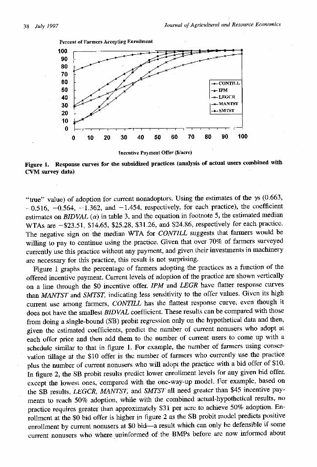
Figure 1. Response curves for the subsidized practices (analysis of actual users combined with

CVM survey data)

"true" value) of adoption for current nonadoptors. Using the estimates of the ys (0.663,

-0.516, -0.564, -1.362, and -1.454, respectively, for each practice), the coefficient

estimates on BIDVAL (a) in table 3, and the equation in footnote 5, the estimated median

WTAs are -$23.51, $14.65, $25.28, $31.26, and $24.86, respectively for each practice.

The negative sign on the median WTA for CONTILL suggests that farmers would be

willing to pay to continue using the practice. Given that over 70% of farmers surveyed

currently use this practice without any payment, and given their investments in machinery

are necessary for this practice, this result is not surprising.

Figure 1 graphs the percentage of farmers adopting the practices as a function of the

offered incentive payment. Current levels of adoption of the practice are shown vertically

on a line through the $0 incentive offer. IPM and LEGR have flatter response curves

than MANTST and SMTST, indicating less sensitivity to the offer values. Given its high

current use among farmers, CONTILL has the flattest response curve, even though it

does not have the smallest BIDVAL coefficient. These results can be compared with those

from doing a single-bound (SB) probit regression only on the hypothetical data and then,

given the estimated coefficients, predict the number of current nonusers who adopt at

each offer price and then add them to the number of current users to come up with a

schedule similar to that in figure 1. For example, the number of farmers using conser-

vation tillage at the $10 offer is the number of farmers who currently use the practice

plus the number of current nonusers who will adopt the practice with a bid offer of $10.

In figure 2, the SB probit results predict lower enrollment levels for any given bid offer,

except the lowest ones, compared with the one-way-up model. For example, based on

the SB results, LEGCR, MANTST, and SMTST all need greater than $45 incentive pay-

ments to reach 50% adoption, while with the combined actual-hypothetical results, no

practice requires greater than approximately $31 per acre to achieve 50% adoption. En-

rollment at the $0 bid offer is higher in figure 2 as the SB probit model predicts positive

enrollment by current nonusers at $0 bid-a result which can only be defensible if some

current nonusers who where uninformed of the BMPs before are now informed about

38 July 1997

I


Percent of Farmers Accepting EnrollmentI UU

9080706050403020100

0 10 20 30 40 50 60 70 80 90 100

Incentive Payment Offer ($/acre)

Figure 2. Response curves for the subsidized practices (analysis of CVM survey data only)

them and may use them even at $0 bid-while the OWU model predicts only current(actual) use at $0 bid and hence is more conservative.

Continuous Model Combining the Actual and Hypothetical Data

The next step is to incorporate the one-way-up results into a continuous model regression,a regression with acres on which the practices are used as the dependent variable. Spe-cifically, the dependent variable is stated acres allocated to the practice for current non-users of the practice and actual acres allocated to the practice for current users, whichfor farmer i can be stated as:

(4) PACRESi = z I 0 + ui,

where PACRESi is the amount of acres in the preferred practice, zi is a vector of ex-planatory variables, and u, is a disturbance with mean zero. As with the discrete choicemodel, the decision on which variables to include in the regressions for each of thepractices was based on whether or not the variables appear justified from a farm man-agement standpoint. Since economic theory does not suggest any a priori reasons whythe PACRES equation should have different explanatory variables than the adoptionequation, the same variables are used. To reduce the potential of some possible form ofheteroskedasticity associated with the total acreage (TACRE) variable, PACRESi is di-vided by TACREi for the regressions.

Ordinary least squares (OLS) estimates of (4) may be biased. Because PACRESi isonly observed for the farmers who are current users or are willing to adopt at the offeredincentive payment, the sample for the regression equation may not be drawn randomlyfrom the population who answered the survey, implying sampling bias due to omittedPACRESi. In addition to being potentially biased, OLS estimates are inefficient (Greene1990). The Heckit procedure (Greene 1990) can be used to correct (4) for nonrandomsampling by using information from the one-way-up qualitative variable regression. Since

Cooper

I~~~~~~~~~~~~~~~~~~~~~~~~~~~~~~~


PACRESi is observed only when yi = 1 (for current users and for hypothetical users),(4) should be rewritten as:

(5) E[PACRESi zi, in sample] = E[PACRESi zi, Yi = 1],

= E[PACRESIz i, ei > AV i], or

= zi + E[uei i AVi].

To estimate this continuous model in a sample selection framework, the Mills ratio

calculated from the one-way-up model is added as an explanatory variable (Greene

1990). Variables which are highly correlated (using a standard of correlation coefficientgreater than or equal to 0.5) with the Mills ratio explanatory variables are removed,resulting in one or two variables being removed from each continuous model equation.

Because the dependent variable PACRES/TACREi is censored to fall between 0 and

1, OLS estimation of the above Heckit model may be biased and inconsistent. Hence, a

tobit version of the Heckit model is estimated with the lower and upper limits set at 0and 1, respectively. To correct for heteroskedasticity between users and nonusers, the

variance of the error term is var(e) = o2eylZi, where zi = 1 if respondent i is a nonuser

and 0 if a user. 10

The tobit model results are presented in table 4. For four of the five BMPs, thecoefficient on BIDVAL is significant and of the expected sign, either through its impact

in the Mills ratio (as in CONTILL) or through the BIDVAL (for practices LEGCR,

MANTST, and SMTST). Note that for the Mills ratio variable A,, aAIaBIDVALi is negative.

Based on the results from table 3, the negative sign on the Mills ratio coefficient for

CONTILL shows the expected result that an increase in the cost share for conservationtillage leads to an increase in the percentage of total acres on which conservation tillage

is used. For the other BMPs, since the Mills ratio is not significant, sample selectionbias is unlikely to be a concern. A large majority of the farmers in the sample use

conservation tillage, while a minority of farmers use the other practices, which may have

some bearing on producing significant sample selection bias in the former but not in thelatter. Of the other explanatory variables, none was significant for every practice, imply-

ing that the relevant set of explanatory variables differs for each practice. For example,

the coefficient on ANIMAL was significant and negative for four of the five cases, sug-gesting logically that farmers with animal operations are less likely to be interested in

using the offered practices. However, ANIMAL is not significantly different from 0 in

the manure testing (MANTST) practice; while a positive coefficient may be predicted a

priori, a negative sign would have been quite unusual. On the other hand, the coefficient

on MANURE (farmer applies manure to field) is significant only for MANTST and is

positive, which is not surprising as one could expect that farmers who apply manure to

their fields may have a strong interest in MANTST.As expected, since a great majority of farmers already use conservation tillage, the

CONTILL equation is not particularly sensitive to the cost-share offer. An increase in the

cost share from the current level of $0 to $10 results in only 2.6% more acres using the

practice. On the other hand, for manure testing, which is currently used by a small

10 Note that var(e) cannot be written as o2evo+vlz where zi = 1 if respondent is a nonuser and 0 if respondent is a user. In

the Limdep 6.0 (Greene 1992) tobit model with heteroskedasticity correction we used, yo needs to be set equal to 0 since or

is a free parameter in this program, and thus, the inclusion of a constant in the variance of the error term model will cause

a singular covariance matrix.

40 July 1997


Table 4. Tobit Continuous Stage Regression for Acreage under BMP

Coefficient Estimates

Variables CONTILL IPM LEGCR MANTST SMTST

CONSTANT

BIDVAL

EDUC

TISTST

HEL

EXPER

PESTM

ROTATE

MANURE

ANIMAL

FLVALUE

SNT

IA

ALBR

IDAHO

BPWORK

NETINC

MILLS

FMUSE

Sigma

Obs.Sum lnLSum lnL

w/out Mills

63.53(5.8)

-0.45(-1.2)

0.31(0.3)

0.59(0.2)

-0.24(-2.4)

-1.34(-0.4)-4.67

(-0.9)1.58

(0.4)-6.59

(-2.0)0.00

(2.4)

13.46(1.7)

-22.05(-2.8)

16.47(2.6)

-0.01(-0.6)

0.00(-0.8)-20.87(-2.1)-11.11(-0.9)

35.75(8.7)

794-307.9

-310.2

44.49(4.4)0.24(0.7)

-0.27(-1.5)

4.55(1.0)3.15

(0.4)

-17.15(-2.9)

0.00(1.5)

33.20(4.4)2.76

(0.4)28.24(3.7)0.01

(0.5)0.00

(-0.2)7.31

(0.9)4.35

(0.4)

32.34(10.7)366

-166.1

-166.6

43.42(2.9)1.25

(2.7)-1.95(-1.0)

2.25(0.3)

-0.19(-1.0)

2.62(0.3)7.33

(1.0)-9.84

(-1.6)0.01

(3.7)8.62

(1.1)

7.92(1.4)0.10

(2.5)0.00

(-0.2)-9.34

(-1.1)-16.39(-1.1)

42.33(7.2)

291-145.4

-146.3

33.43(1.6)1.34

(2.4)-2.51

(-1.0)26.35(1.7)

-0.52(-1.5)

-5.76(-0.4)

45.23(4.8)

-3.35(-0.4)

0.00(0.3)

-13.22(-1.4)

-7.65(-0.6)

19.16(1.5)0.06

(1.2)0.00

(-1.4)9.70

(0.7)-32.51(-1.9)

37.95(7.4)

128-49.6

-50.0

55.39(2.4)0.84

(1.6)-2.69

(-1.2)

-0.28(-1.0)

-0.19(-0.0)

-26.09(-3.0)

0.00(0.0)

18.73(1.8)

25.51(2.6)0.11

(2.1)0.00

(-0.6)5.37

(0.6)9.36

(0.5)

32.33(8.7)

159-71.7

-71.9

Notes: The figures in parentheses are coefficients/standard errors. Dependent variable = (actual orhypothetical acres the practice is used on)/(total farm acreage), where tobit lower and upper limits areset to 0 and 1, respectively. Coefficients are scaled up by a factor of 100 for ease of presentation.

Cooper


percentage of farmers, an increase in the cost share from the current level of $0 to $10

results in 13.3% more acres using the practice. Legume crediting (LEGCR) shows similarincreases over the same offer range, while soil moisture testing (SMTST) shows an 8.4%increase and IPM a 2.4% increase.

Conclusion

Using farmer responses to CVM survey data from four watershed regions in the United

States, I estimate the minimum incentive payments a farmer would accept in order to

adopt more environmentally friendly best management practices. In a departure from the

traditional CVM survey approach, since data on actual users of the BMPs (i.e., farmerswho currently use the BMPs with no incentive payments or, in other words, at $0 bidoffers) exist, I extend the traditional CVM survey analysis by combining this actual

market data with the hypothetical, or contingent behavior analysis. Doing so, I add in-formation to the regression, thereby most likely increasing the reliability of the resultscompared with that from the contingent behavior survey response data only. From apolicy standpoint, getting relevant farmers to adopt the BMPs is likely the most difficulthurdle. However, what also matters from an environmental standpoint is how many acres

are enrolled in the practice, given the decision to participate. Hence, given the results

from the adoption equations, I also model the number of acres enrolled in the BMPs as

a function of the incentive payments. As with the discrete choice functions, I combinethe actual and the contingent behavior data.

For the data sets used in this article, adoption rates predicted with the combined datamodel are significantly higher over a wide range of offers than those predicted using a

single-bound probit analysis of the hypothetical data only. Hence, using the traditional

CVM analysis results to determine payments to attain a given level of adoption may

result in overpayment. Still, the high cost to the government of attaining much higherthan current levels of adoption suggests that incentive payments may not be a particularlyfeasible policy option in this period of shrinking agricultural budgets. This hypothesis is

only enforced by the somewhat flat response the bid offers in terms of the number ofacres enrolled given the decision to adopt the practice. However, we need more infor-mation on the valuation of the environmental benefits of adopting the BMPs in order to

know whether the incentive payment schemes can yield benefits greater than costs forany of the BMPs. If incentive payment schemes are used to promote adoption, basingpayments on the combined data model instead of the contingent behavior data only modelcan result in substantial cost savings for the government.

[Received October 1995; final version received January 1997.]

References

Adamowicz, W. L., J. Louviere, and M. Williams. "Combining Stated and Revealed Preference Methods for

Valuing Environmental Amenities." J. Environ. Econ. and Manage. 26(1994):271-92.

Cooper, J. "Optimal Bid Selection for Dichotomous Choice Contingent Valuation Surveys." J. Environ. Econ.

and Manage. 24(1993):25-40.

42 July 1997


Craig, L., J. Boyce, and K. Criddle. "Economic Valuation of the Chinook Salmon Sport Fishery of the GulkanaRiver, Alaska, under Current and Alternative Management Plans." Land Econ. 72(1996):113-28.

Feather, P, and J. Cooper. "Strategies for Curbing Water Pollution." Agr. Outlook 224(November 1995):19-22.Greene, W. Econometric Analysis. New York NY: MacMillan Publishing Company, 1990.

.Limdep: User's Manual and Reference Guide, Version 6.0. Bellport NY: Econometric Software, Inc.,1992.

Hanemann, M. "Welfare Evaluations in Contingent Valuation Experiments with Discrete Response Data."Amer. J. Agr. Econ. 66,3(1984):332-41.

. "Welfare Evaluations in Contingent Valuation Experiments with Discrete Response Data: Reply."Amer. J. Agr. Econ. 71,4(1989):1057-61.

Hanemann, M., J. Loomis, and B. Kanninen. "Statistical Efficiency of Double-Bound Dichotomous ChoiceContingent Valuation." Amer. J. Agr. Econ. 73,4(1991):1255-263.

Hoehn, J., and A. Randall. "A Satisfactory Benefit Cost Estimator from Contingent Valuation." J. Environ.Econ. and Manage. 12(1987):226-47.

Kanninen, B. "Optimal Experimental Design for Double-Bounded Dichotomous Choice Contingent Valua-tion." Land Econ. 69,2(1993):138-46.

Sinner, J. "We Can Get More for Our Tax Dollars." Choices 5(2nd Quart. 1990):10-13.U.S. Department of Commerce, National Oceanic and Atmospheric Administration. "Proposed Rules: Natural

Resource Damage Assessment." Federal Register 58,10 (1993):4601-614.

Appendix: Example of Survey Questions for Adoption of a Practice

a. Is this practice currently in use on your farm? [Enter 1 if Yes. If No, please skip toitem e.]

b. When did you begin using this practice? [Please enter approximate month and year,for example 0190 for January of 1990.]

c. Was this practice cost-shared when you adopted it? [If YES enter dollars per acre(total cash share for cols. 10-12). If NO leave blank.]

d. On how many acres do you use this practice? [Enter number of acres and skip toitem j.]

e. Would you adopt this practice if you received a $24/acre incentive to do so? [Enter1 if Yes.]

f. How many acres would you apply this practice on?

Cooper

combining actual and contingent behavior data to model

Documents