Combined LectureCS621: Artificial Intelligence (lecture 25)CS626/449: Speech-NLP-Web/Topics-in-

AI (lecture 26)

Pushpak BhattacharyyaComputer Science and Engineering Department

IIT Bombay

Forward Backward probability;Viterbi Algorithm

Another Example

Urn 1# of Red = 30

# of Green = 50 # of Blue = 20

Urn 3# of Red =60

# of Green =10 # of Blue = 30

Urn 2# of Red = 10

# of Green = 40 # of Blue = 50

A colored ball choosing example :

U1 U2 U3

U1 0.1 0.4 0.5

U2 0.6 0.2 0.2

U3 0.3 0.4 0.3

Probability of transition to another Urn after picking a ball:

Example (contd.)

U1 U2 U3

U1 0.1 0.4 0.5

U2 0.6 0.2 0.2

U3 0.3 0.4 0.3

Given :

Observation : RRGGBRGR

State Sequence : ??

Not so Easily Computable.

and

R G B

U1 0.3 0.5 0.2

U2 0.1 0.4 0.5

U3 0.6 0.1 0.3

Example (contd.)

• Here : – S = {U1, U2, U3}– V = { R,G,B}

• For observation:– O ={o1… on}

• And State sequence– Q ={q1… qn}

• π is

U1 U2 U3

U1 0.1 0.4 0.5

U2 0.6 0.2 0.2

U3 0.3 0.4 0.3

R G B

U1 0.3 0.5 0.2

U2 0.1 0.4 0.5

U3 0.6 0.1 0.3

A =

B=

)( 1 ii UqP

Hidden Markov Models

Model Definition

• Set of states : S where |S|=N• Output Alphabet : V• Transition Probabilities : A = {aij}

• Emission Probabilities : B = {bj(ok)}

• Initial State Probabilities : π),,( BA

Markov Processes

• Properties– Limited Horizon :Given previous n states, a state i,

is independent of preceding 0…i-n+1 states.• P(Xt=i|Xt-1, Xt-2 ,… X0) = P(Xt=i|Xt-1, Xt-2… Xt-n)

– Time invariance : • P(Xt=i|Xt-1=j) = P(X1=i|X0=j) = P(Xn=i|X0-1=j)

Three Basic Problems of HMM1. Given Observation Sequence O ={o1… oT}

– Efficiently estimate P(O|λ)

2. Given Observation Sequence O ={o1… oT}– Get best Q ={q1… qT} i.e.

• Maximize P(Q|O, λ)

3. How to adjust to best maximize – Re-estimate λ

),,( BA )|( OP

Three basic problems (contd.)

• Problem 1: Likelihood of a sequence– Forward Procedure– Backward Procedure

• Problem 2: Best state sequence– Viterbi Algorithm

• Problem 3: Re-estimation– Baum-Welch ( Forward-Backward Algorithm )

Problem 2

• Given Observation Sequence O ={o1… oT}– Get “best” Q ={q1… qT} i.e.

• Solution :1. Best state individually likely at a position i2. Best state given all the previously observed states

and observations Viterbi Algorithm

Example

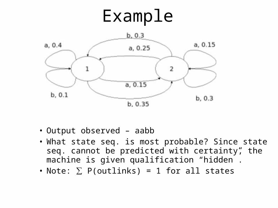
• Output observed – aabb • What state seq. is most probable? Since state seq. cannot

be predicted with certainty, the machine is given qualification “hidden”.

• Note: ∑ P(outlinks) = 1 for all states

Probabilities for different possible seq1

1,21,10.4

1,1,10.16 1,1,20.06 1,2,1 0.0375 1,2,20.0225

1,1,1,1

0.016

1,1,1,2

0.056

...and so on

1,1,2,1

0.018

1,1,2,2

0.018

0.15

IfP(si|si-1, si-2) (order 2 HMM)

then the Markovian assumption will take effect only after two levels.(generalizing for n-order… after n levels)

Viterbi for higher order HMM

Forward and Backward Probability Calculation

A Simple HMM

q r

a: 0.3

b: 0.1

a: 0.2

b: 0.1

b: 0.2

b: 0.5

a: 0.2

a: 0.4

Forward or α-probabilities

Let αi(t) be the probability of producing w1,t-1, while ending up in state si

αi(t)= P(w1,t-1,St=si), t>1

Initial condition on αi(t)

αi(t)=

1.0 if i=1

0 otherwise

Probability of the observation using αi(t)

P(w1,n)

=Σ1 σ P(w1,n, Sn+1=si)

= Σi=1 σ αi(n+1)

σ is the total number of states

Recursive expression for α

αj(t+1)

=P(w1,t, St+1=sj)

=Σi=1 σ P(w1,t, St=si, St+1=sj)

=Σi=1 σ P(w1,t-1, St=sj)

P(wt, St+1=sj|w1,t-1, St=si)

=Σi=1 σ P(w1,t-1, St=si)

P(wt, St+1=sj|St=si)

= Σi=1 σ αj(t) P(wt, St+1=sj|St=si)

Time Ticks 1 2 3 4 5

INPUT ε b

bb bbb bbba

1.0 0.2 0.05 0.017 0.0148

0.0 0.1 0.07 0.04 0.0131

P(w,t) 1.0 0.3 0.12 0.057 0.0279

)(tq

)(tr

The forward probabilities of “bbba”

Backward or β-probabilities

Let βi(t) be the probability of seeing wt,n, given that the state of the HMM at t is si

βi(t)= P(wt,n,St=si)

Probability of the observation using β

P(w1,n)=β1(1)

Recursive expression for β

βj(t-1)

=P(wt-1,n |St-1=si)

=Σj=1 σ P(wt-1,n, St=sj |St-1=si)

=Σj=1 σ P(wt-1, St=sj|St-1=si) P(wt,n,|wt-1,St=sj, St-1=si)

=Σj=1 σ P(wt-1, St=sj|St-1=si) P(wt,n, |St=sj)

(consequence of Markov Assumption)= Σj=1

σ P(wt-1, St=sj|St-1=si) βj(t)

Forward Procedure

model given the ,...n observatio partial theof and

, is position at state y that theprobabilit The

)|,...()(

as variableForward Define

1

1

t

i

ittt

oo

St

SqooPi

Forward Step:

Forward Procedure

Backward Procedure

Backward Procedure

Forward Backward Procedure

• Benefit– Order

• N2T as compared to 2TNT for simple computation

• Only Forward or Backward procedure needed for Problem 1

Problem 2

• Given Observation Sequence O ={o1… oT}– Get “best” Q ={q1… qT} i.e.

• Solution :1. Best state individually likely at a position i2. Best state given all the previously observed states

and observations Viterbi Algorithm

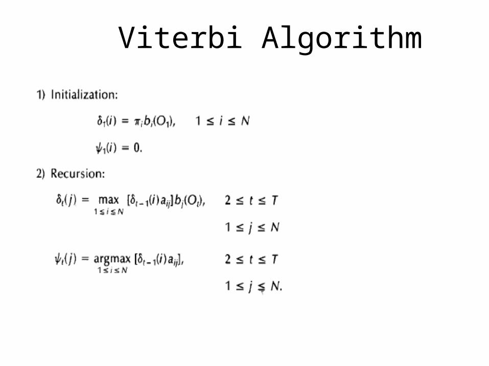
Viterbi Algorithm• Define such that,

i.e. the sequence which has the best joint probability so far.

• By induction, we have,

Viterbi Algorithm

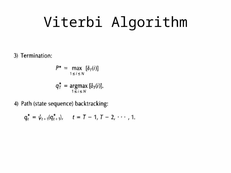
Viterbi Algorithm

Problem 3

• How to adjust to best maximize – Re-estimate λ

• Solutions :– To re-estimate (iteratively update and improve)

HMM parameters A,B, π• Use Baum-Welch algorithm

),,( BA )|( OP

Baum-Welch Algorithm

• Define

• Putting forward and backward variables

Baum-Welch algorithm

• Define

• Then, expected number of transitions from Si

• And, expected number of transitions from Sj to Si

Baum-Welch Algorithm

• Baum et al have proved that the above equations lead to a model as good or better than the previous