Combined Control Strategies for Controlling

the Trajectory of a Quadcopter

Viviana Moya #1, Vanessa Espinosa #2, Danilo Chávez #3, Oscar Camacho #,*4, Paulo Leica#5

#Departamento de Automatización y Control Industrial, Escuela Politécnica Nacional, Quito, Ecuador

(viviana.moya, vanessa.espinosa, danilo.chavéz, oscar.camacho, paulo.leica)@epn.edu.ec

* Universidad de los Andes, Mérida, Venezuela ocamacho@ula.ve

Abstract—The aim of this paper is to show the design of a

combined controller, using Backstepping and sliding mode

control concepts, for controlling the trajectory following of a

quadcopter. The Backstepping-sliding mode controller is

compared against a Backstepping- PID controller for circular

trajectory. The results by simulations demonstrated the

advantages of the proposed approach. The ISE performance

index is used to measure the performance and robustness of

both controllers.

Resumen— El objetivo de este proyecto es mostrar el diseño

de un control combinado utilizando los conceptos de

Backstepping y Control de Modos Deslizantes para el control de

seguimiento de trayectoria de un cuadricóptero. El controlador

Backstepping-Modos Deslizantes es comparado con un

controlador Backstepping-PID en una trayectoria circular. Los

resultados de las simulaciones demuestran las ventajas del

enfoque propuesto. El índice de rendimiento ISE se utiliza para

medir el desempeño y la robustez de los dos controladores.

I. INTRODUCTION

A quadcopter is an UAV (Unmanned Aerial Vehicle),

used in many fields such as ground exploration, data

collection and monitoring in areas as diverse as military,

research, agriculture, maintenance and security among many

more [1]. In order of making those tasks in the best possible way, it

is important the development of control mechanisms that

seek to ensure the smooth implementation of trajectories

planned by the operators.

Due to the complexity of the dynamical system that

governs the behaviour of a quadcopter, most of the controller

approaches are not able to stabilize properly the position or

follow the desired trajectory ([2], [3])

Some works related with this topic have been presented.

Arellano-Muro, Carlos Vega, Luis Castillo,B. and Loukianov,

Alexander [4], proposed a Backstepping control to solve the

trajectory tracking problem and ensures robustness against

external forces and parameters variations.

Kacimi, Mokhtari and Kouadri [5], presented in their

paper a sliding mode controller to guarantee Lyapunov

stability and synthesize tracking errors. It takes into account

nonlinearities.

Ramirez, Parra, Sánchez, and Garcia [6], developed a new

control technique for handling the aerodynamic forces. The

controller is composed by a Backstepping that is used to

stabilize the system and also by a sliding mode which

compensates the disturbances.

Bouabdallah and Siegwart [7], proposed two nonlinear

control techniques and applied them to an autonomous micro

helicopter called Quadrotor. A backstepping and a sliding-

mode techniques. They performed various simulations in

open and closed loop and also implemented several

experiments on the test-bench to validate the control laws.

In this work, it is presented a control scheme that combines

two controller’s approaches. The combined controller

approach is composed by two components. The first part is a

Backstepping controller, its objective is to create a virtual

control law which permits to calculate the new references for

controlling roll and pitch angles. Secondly, a sliding mode

controller is used, it executes control over the rotor and thus

allows stabilization of the position and the appropriate

monitoring of the planned trajectory to follow. The

references for the sliding mode controller are provided by the

Backstepping control. Then, the proposed algorithm is

compared against a Backstepping-PID controller by

simulations.

The combination of both schemes should produce a

controller approach to strengthen and to improve the

performance and robustness of both controllers. The system’s

performance is tested and ISE performance index used to

measure it.

This article is organized as follows. Section 2 presents the

dynamic model of the quadcopter. Section 3 explains the

basic concepts about sliding mode and Backstepping

controllers. Section 4 shows the design of the controllers.

Section 5 presents the results of the simulations tests using

the designed controllers. Finally, section 6 presents the

conclusions of this work.

II. DYNAMIC MODEL OF A QUADCOPTER

The quadcopter can be seen as a multivariable system

having six degrees of freedom which correspond to three

translational (x, y, 𝑧) and three rotational (∅, 𝜃, 𝜓). The quadcopter has four arms forming a cross, located at

each end there are four actuators each one form by a motor

and a propeller (two rotate clockwise and two in the opposite

direction). The quadcopter has three types of motion: roll (∅),

pitch (𝜃) and yaw (𝜓). Quadcopter position is controlled by

changing the speed at which the rotors rotate.

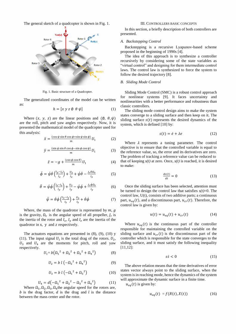
The general sketch of a quadcopter is shown in Fig. 1.

Fig. 1. Basic structure of a Quadcopter.

The generalized coordinates of the model can be written

as:

ℎ = [𝑥 𝑦 𝑧 ∅ 𝜃 𝜓] (1)

Where (𝑥, 𝑦, 𝑧) are the linear positions and (∅, 𝜃, 𝜓)

are the roll, pitch and yaw angles respectively. Now, it is

presented the mathematical model of the quadcopter used for

this analysis:

�̈� =(cos 𝜓 sin 𝜃 cos 𝜙+sin 𝜓 sin 𝜙)

𝑚𝑈1 (2)

�̈� =(sin 𝜓 sin 𝜃 cos 𝜙−sin 𝜙 cos 𝜓)

𝑚𝑈1 (3)

�̈� = −𝑔 +(cos 𝜙 cos 𝜃)

𝑚𝑈1 (4)

�̈� = �̇��̇� (𝐼𝑦−𝐼𝑧

𝐼𝑥) +

𝑈2

𝐼𝑥+ �̇��̇� −

𝐽𝑟�̇�Ω𝑟

𝐼𝑥 (5)

�̈� = �̇��̇� (𝐼𝑧−𝐼𝑥

𝐼𝑦) +

𝑈3

𝐼𝑦− �̇��̇� +

𝐽𝑟�̇�Ω𝑟

𝐼𝑦 (6)

�̈� = �̇��̇� (𝐼𝑥−𝐼𝑦

𝐼𝑧) +

𝑈4

𝐼𝑧+ �̇��̇� (7)

Where, the mass of the quadrotor is represented by 𝑚, 𝑔

is the gravity, Ωr is the angular speed of all propeller, 𝐽𝑟 is

the inertia of the rotor and 𝐼𝑥, 𝐼𝑦 and 𝐼𝑧 are the inertia of the

quadrotor in x, y and 𝑧 respectively.

The actuators equations are presented in (8), (9), (10) y

(11). The input signal 𝑈1 is the total drag of the rotors. 𝑈2,

𝑈3 and 𝑈4 are the moments for pitch, roll and yaw

respectively.

𝑈1= 𝑏(Ω12 + Ω2

2 + Ω32 + Ω4

2) (8)

𝑈2 = 𝑏 𝑙 (−Ω22 + Ω4

2) (9)

𝑈3 = 𝑏 𝑙 (−Ω12 + Ω3

2) (10)

𝑈4 = 𝑑(−Ω12 + Ω2

2 − Ω32 + Ω4

2) (11)

Where Ω1, Ω2, Ω3, Ω4the angular speed for the rotors are,

𝑏 is the drag factor, 𝑑 is the drag and 𝑙 is the distance

between the mass center and the rotor.

III. CONTROLLERS BASIC CONCEPTS

In this section, a briefly description of both controllers are

presented.

A. Backstepping Control

Backstepping is a recursive Lyapunov-based scheme

proposed in the beginning of 1990s [4].

The idea of this approach is to synthesize a controller

recursively by considering some of the state variables as

“virtual control” and designing for them intermediate control

laws. The control law is synthesized to force the system to

follow the desired trajectory [8].

B. Sliding Mode Control

Sliding Mode Control (SMC) is a robust control approach

for nonlinear systems [9]. It faces uncertainty and

nonlinearities with a better performance and robustness than

classic controllers.

The sliding mode control design aims to make the system

states converge to a sliding surface and then keep on it. The

sliding surface 𝑠(𝑡) represents the desired dynamics of the

system, which is defined [10] by:

𝑠(𝑡) = �̇� + 𝜆𝑒 (12)

Where 𝜆 represents a tuning parameter. The control

objective is to ensure that the controlled variable is equal to

the reference value, so, the error and its derivatives are zero.

The problem of tracking a reference value can be reduced to

that of keeping s(t) at zero. Once, s(t) is reached, it is desired

to make:

𝑑𝑠(𝑡)

𝑑𝑡= 0 (13)

Once the sliding surface has been selected, attention must

be turned to design the control law that satisfies s(t)=0. The

control law, U(t), consists of two additive parts; a continuous

part, 𝑢𝑒𝑞(𝑡), and a discontinuous part, 𝑢𝑐𝑟(𝑡). Therefore, the

control law is given by:

𝑢(𝑡) = 𝑢𝑒𝑞(𝑡) + 𝑢𝑐𝑟(𝑡) (14)

Where 𝑢𝑒𝑞(𝑡) is the continuous part of the controller

responsible for maintaining the controlled variable on the

sliding surface and 𝑢𝑐𝑟(𝑡) is the discontinuous part of the

controller which is responsible for the state converges to the

sliding surface, and it must satisfy the following inequality

[11,12]:

𝑠�̇� < 0 (15)

The above relation means that the time derivatives of error

states vector always point to the sliding surface, when the

system is in reaching mode, hence the dynamics of the system

will approximate the dynamic surface in a finite time.

𝑢𝑒𝑞(𝑡) is given by:

𝑢𝑒𝑞(𝑡) = 𝑓(𝑅(𝑡), 𝑋(𝑡)) (16)

Where 𝑅(𝑡) is the reference signal and 𝑋(𝑡) is the model

output, 𝑢𝑒𝑞(𝑡) will be determined later using the equivalent

control procedure [9] . 𝑢𝑐𝑟(𝑡) has a non-linear element that

includes the switching element of the control’s law [9, 10]

𝑢𝑐𝑟(𝑡) = 𝐾𝐷𝑠𝑖𝑔𝑛(𝑠(𝑡)) (17)

To smooth the discontinuity, a sigmoid function is used

[11]:

𝑢𝑐𝑟(𝑡) = 𝐾𝐷𝑠(𝑡)

|𝑠(𝑡)|+𝛿 (18)

Where 𝐾𝐷 is a tuning parameter responsible for the speed

adjustment, and δ is a parameter responsible for reducing

high frequency oscillations around the desired equilibrium

point, these undesirable oscillations are known as chattering

[9, 11, 12].

IV. CONTROLLERS

The quadcopter has six degrees of freedom, with input

signals which are responsible for making it moves forward,

backward, right and left, up or down. To control the system,

four equations to be connected to 𝑈1, 𝑈2, 𝑈3 and 𝑈4 were

designed.𝑈1 defines the altitude reference and 𝑈2, 𝑈3 and 𝑈4

define quadcopter roll, pitch and yaw references.

The next part presents the development of both controllers.

Firstly, the Backstepping is shown and secondly, the sliding

mode is treated.

A. Backstepping Control Translation System

Considering 𝑢𝑥 = cos 𝜓 sin 𝜃 cos 𝜙 + sin 𝜓 sin 𝜙 and

𝑢𝑦 = sin 𝜓 sin 𝜃 cos 𝜙 − sin 𝜙 cos 𝜓 and replacing them

into Eq. (2) and Eq. (3), [7]:

�̈� =𝑈1

𝑚𝑢𝑥 (19)

�̈� = 𝑈1

𝑚𝑢𝑦 (20)

1) Position X

The Backstepping control procedure to design the

controllers for translation system is presented in [4].

Position error 𝑋 is given by:

𝑒𝑥 = 𝑥𝑟𝑒𝑓 − 𝑥 (21)

Differentiating the previous equation:

�̇�𝑥 = �̇�𝑟𝑒𝑓 − �̇� (22)

The goal is to design a virtual control 𝑥∗ which makes

𝑙𝑖𝑚𝑡 →∞

𝑒𝑥 → 0, considering the Lyapunov function 𝑉𝑥:

𝑉𝑥 =1

2𝑒𝑥

2 > 0 (23)

And the derivate of this function is:

�̇�𝑥 = 𝑒𝑥�̇�𝑥 = 𝑒𝑥(�̇�𝑟𝑒𝑓 − �̇�) (24)

Introducing the virtual control:

𝑥∗ = �̇�𝑟𝑒𝑓 + 𝑞𝑒𝑥 (25)

Where 𝑞 is a positive constant value. Defining a new

variable:

𝑒𝑥1 = 𝑥∗ − �̇� = �̇�𝑟𝑒𝑓 + 𝑞𝑒𝑥 − �̇� (26)

Rearranging Eq. (26), it is obtained:

�̇�𝑟𝑒𝑓 = 𝑒𝑥1 − 𝑞 𝑒𝑥 + �̇� (27)

By replacing Eq. (27) into Eq. (24) the following result is

obtained:

�̇�𝑥 = 𝑒𝑥(𝑒𝑥1 − 𝑞 𝑒𝑥 + �̇� − �̇�) = −𝑞𝑒𝑥2 + 𝑒𝑥𝑒𝑥1

(28)

The derivative of Eq. (26) is:

�̇�𝑥1 = �̈�𝑟𝑒𝑓 + 𝑞�̇�𝑥 − �̈� (29)

Replacing Eq. (19) in Eq. (29), it is obtained:

�̇�𝑥1 = �̈�𝑟𝑒𝑓 + 𝑞�̇�𝑥 −𝑈1

𝑚𝑢𝑥 (30)

In order to get lim𝑡 →∞

𝑒𝑥1 → 0 , it is necessary to choose a

𝑉𝑥𝑥 Lyapunov control function:

𝑉𝑥𝑥 = 𝑉𝑥 +1

2𝑒𝑥1

2 > 0 (31)

Obtaining the derivate we have:

�̇�𝑥𝑥 = �̇�𝑥 + 𝑒𝑥1�̇�𝑥1 (32)

Replacing equation Eq. (29) in Eq. (32), it is obtained:

�̇�𝑥𝑥 = �̇�𝑥 + 𝑒𝑥1 (�̈�𝑟𝑒𝑓 + 𝑞�̇�𝑥 −𝑈1

𝑚𝑢𝑥) (33)

Substituting Eq. (28) in Eq. (33):

�̇�𝑥𝑥 = −𝑞𝑒𝑥2 + 𝑒𝑥𝑒𝑥1 + 𝑒𝑥1 (�̈�𝑟𝑒𝑓 + 𝑞�̇�𝑥 −

𝑈1

𝑚𝑢𝑥) (34)

It is proposed that:

𝑢𝑥∗ =

𝑚

𝑈1[�̈�𝑟𝑒𝑓 + 𝑞�̇�𝑥 + 𝑒𝑥 + 𝑝𝑒𝑥1] (35)

Assuming now perfect velocity tracking 𝑢𝑥 ≅ 𝑢𝑥∗, and

replacing Eq. (35) in Eq. (34):

�̇�𝑥𝑥 = −𝑞𝑒𝑥2 − 𝑝𝑒𝑥1

2 < 0 (36)

where 𝑒𝑥 → 0 and 𝑒𝑥1 → 0 with 𝑡 → ∞

Finally, the x control law is:

𝑢𝑥∗ =

𝑚

𝑈1[�̈�𝑟𝑒𝑓 + 𝑞𝑒�̇� + 𝑒𝑥 + 𝑝(�̇�𝑟𝑒𝑓 + 𝑞𝑒𝑥 − �̇�)] (37)

Desired pitch angle

Where the desired pitch angle is 𝜃𝑟𝑒𝑓 . From Eq. (2), 𝜃𝑟𝑒𝑓 .

is obtained:

𝜃𝑟𝑒𝑓 = 𝑠𝑖𝑛−1 (

�̈�𝑚

𝑈1−𝑠𝑖𝑛𝜓𝑠𝑖𝑛𝜙

𝑐𝑜𝑠𝜓𝑐𝑜𝑠𝜙) (38)

Replacing in Eq. (19) in Eq. (38) and considering 𝑢𝑥 ≅𝑢𝑥

∗:

𝜃𝑟𝑒𝑓 = 𝑠𝑖𝑛−1 (𝑢𝑥

∗−𝑠𝑖𝑛𝜓𝑠𝑒𝑛𝜙

𝑐𝑜𝑠𝜓𝑐𝑜𝑠𝜙) (39)

2) Position Y

Following the same procedure for the X control, is

obtained:

𝑢𝑦∗ =

𝑚

𝑈1[�̈�𝑟𝑒𝑓 + 𝑞�̇�𝑦 + 𝑒𝑦 + 𝑝(�̇�𝑟𝑒𝑓 + 𝑞𝑒𝑦 − �̇�)] (40)

Desired roll angle

Where the desired roll angle is 𝜙𝑟𝑒𝑓 . Substituting Eq. (2)

into Eq. (3), 𝜙𝑟𝑒𝑓 is obtained:

𝜙𝑟𝑒𝑓 = 𝑠𝑖𝑛−1 ( 𝑠𝑖𝑛𝜓�̈�𝑚

𝑈1− 𝑐𝑜𝑠𝜓

�̈�𝑚

𝑈1) (41)

Replacing Eq. (19) and Eq. (20), it is obtained:

𝜙𝑟𝑒𝑓 = 𝑠𝑖𝑛−1( 𝑠𝑖𝑛𝜓 𝑢𝑥∗ − 𝑐𝑜𝑠𝜓 𝑢𝑦

∗) (42)

B. Sliding Mode Control (SMC) for Altitude and Rotational

Systems

1) Altitude Control law

The sliding surface is defined in Eq. (12) and Eq. (15). The

error is defined by the difference between the desired altitude

and the quadcopter altitude:

𝑒𝑧 = 𝑧𝑟𝑒𝑓 − 𝑧 (43)

Differentiating the previous equation:

�̇�𝑧 = �̇�𝑟𝑒𝑓 − �̇� (44)

And substituting Eq. (43) and Eq. (44) in Eq. (12):

𝑠 = (�̇�𝑟𝑒𝑓 − �̇�) + 𝜆(𝑧𝑟𝑒𝑓 − 𝑧) (45)

The derivative of the previous equations, is given by:

�̇� = (�̈�𝑟𝑒𝑓 − �̈�) + 𝜆(�̇�𝑟𝑒𝑓 − �̇�) (46)

Using Eq. (4) and replacing in Eq. (46):

�̇� = (�̈�𝑟𝑒𝑓 + 𝑔 −cos 𝜙 cos 𝜃

𝑚𝑈1) + 𝜆(�̇�𝑟𝑒𝑓 − �̇�) (47)

Assuming now perfect velocity tracking 𝑢(𝑡) ≅ 𝑈1, and

using Eq. (14), and replacing 𝑢(𝑡) in 𝑈1:

�̇� = (�̈�𝑟𝑒𝑓 + 𝑔 −cos 𝜙 cos 𝜃

𝑚(𝑢𝑒𝑞 + 𝑢𝑐𝑟)) + 𝜆(�̇�𝑟𝑒𝑓 − �̇�) (48)

To find 𝑢𝑒𝑞 , it is assumed 𝑢𝑐𝑟 = 0 and �̇� = 0, then:

𝑢𝑒𝑞 =𝑚

cos 𝜙 cos 𝜃[�̈�𝑟𝑒𝑓 + 𝑔 + 𝜆(�̇�𝑟𝑒𝑓 − �̇�) ] (49)

To find 𝑢𝑐𝑟, a Lyapunov candidate function is defined by:

𝑉 =1

2𝑠2 > 0 (50)

And its derivate is:

�̇� = 𝑠�̇� < 0 (51)

Replacing Eq. (48) into Eq. (51)

�̇� = 𝑠 ((�̈�𝑟𝑒𝑓 + 𝑔 −cos 𝜙 cos 𝜃

𝑚(𝑢𝑒𝑞 + 𝑢𝑐𝑟)) + 𝜆(�̇�𝑟𝑒𝑓 −

�̇�)) < 0 (52)

Substituting Eq. (49) in Eq. (52)

�̇� = 𝑠 (−cos 𝜙 cos 𝜃

𝑚𝑢𝑐𝑟) = −𝑘𝑐𝑟 𝑠 𝑢𝑐𝑟 < 0 (53)

Where 𝑘𝑐𝑟 =cos 𝜙 cos 𝜃

𝑚 , the 𝜙 and 𝜃 angles are limited to

−𝜋

2< 𝜙 <

𝜋

2 and −

𝜋

2< 𝜃 <

𝜋

2 [13], with this ensures 𝑘𝑐𝑟 >

0.

Rearranging Eq. (53) and for that �̇� < 0, 𝑢𝑐𝑟 is defined

as:

𝑢𝑐𝑟 = 𝑘𝑐𝑟 𝑘𝑑𝑟𝑠𝑖𝑔𝑛(𝑠) ; 𝑘𝑑𝑟 > 0 (54)

To facilitate implementation, it is considered 𝐾𝐷 =𝑘𝑐𝑟𝑘𝑑𝑟 > 0.

Adding Eq. (49) and Eq. (54), and 𝑢(𝑡) ≅ 𝑈1 becomes:

𝑈1 =𝑚

cos 𝜙 cos 𝜃[ 𝑔 + �̈�𝑟𝑒𝑓 + 𝜆(�̇�𝑟𝑒𝑓 − �̇�)] + 𝐾𝐷𝑠𝑖𝑔𝑛(𝑠) (55)

Finally, the altitude control law is:

𝑈1 =𝑚

cos 𝜙 cos 𝜃[ 𝑔 + �̈�𝑟𝑒𝑓 + 𝜆(�̇�𝑟𝑒𝑓 − �̇�)] + 𝐾𝐷

𝑠(𝑡)

|𝑠(𝑡)|+𝛿 (56)

2) Rotational Control law

Following the same procedure for the altitude control, is

obtained the controllers for roll, pitch and yaw:

𝑈2 = 𝐼𝑥 [�̈�𝑟𝑒𝑓 − �̇��̇� (𝐼𝑦−𝐼𝑧

𝐼𝑥) − �̇��̇� +

𝐽𝑟�̇�Ω𝑟

𝐼𝑥+ 𝜆(�̇�𝑟𝑒𝑓 −

�̇�) ] + 𝐾𝐷𝑠(𝑡)

|𝑠(𝑡)|+𝛿 (57)

𝑈3 = 𝐼𝑦 [�̈�𝑟𝑒𝑓 − �̇��̇� (𝐼𝑧−𝐼𝑥

𝐼𝑦) + �̇��̇� −

𝐽𝑟�̇�Ω𝑟

𝐼𝑦+ 𝜆(�̇�𝑟𝑒𝑓 −

�̇�) ] + 𝐾𝐷𝑠(𝑡)

|𝑠(𝑡)|+𝛿 (58)

𝑈4 = 𝐼𝑧 [�̈�𝑟𝑒𝑓 − �̇��̇� (𝐼𝑥−𝐼𝑦

𝐼𝑧) − �̇��̇� + 𝜆(𝜓�̇� − �̇�)] +

𝐾𝐷𝑠(𝑡)

|𝑠(𝑡)|+𝛿 (59)

V. SIMULATION RESULTS

In this section, the servo and regulation tasks for the

quadrotor, for the circular trajectory, are presented, the

quadcopter parameters are presented by [14]. The controllers

were calibrated manually by trial and error. The tuning

parameters for the SMC with Backstepping and the PID

tuning parameters [15] with Backstepping controllers [4] are

shown in the Table I and Table II:

TABLE I SMC AND PID TUNING PARAMETERS

SMC PID

Parameter 𝝀 𝜹 𝒌𝑫 𝒌𝒑 𝒌𝒅 𝒌𝒊

𝑧 7 0.25 50 65 10 14

𝜙 3 0.5 3.5 85 10 5

𝜃 3 0.5 3.5 85 10 5

𝜓 5 0.2 5 65 10 10

TABLE II

BACKSTEPPING CONTROL TUNING PARAMETERS FOR SMC

AND PID

SMC PID

Parameter 𝒑 𝒒 𝒑 𝒒

𝑥 2 10 5 2

𝑦 2 10 5 2

A. Comparison SMC vs PID

In order to evaluate the performance of the SMC controller,

it is compared against a PID controller.

Fig. 2 depicts the results for both controllers for a circular

trajectory. ISE [15, 16] is used to measure the performance

of both controllers. In Table III are shown the ISE and

∆% for circular trajectory

∆% is defined as follows:

∆% = |ISE1−ISE2

(ISE1+ISE2

2)| ∗ 100 (60)

Fig. 2. Circular Trajectory without disturbances.

TABLE III ISE FOR CIRCULAR TRAJECTORY

Parameter

(ISE) 𝐒𝐌𝐂 𝐏𝐈𝐃 ∆%

𝑥 0,63 0,84 29,15

𝑦 0,69 0,86 22,30

𝑧 0,30 0,34 13,08

The results for a circular trajectory with disturbances are

shown in Fig. 3

Fig. 3. Circular Trajectory with external perturbations.

B. Robustness Test

In this part robustness tests are presented. Some changes

in mass are considered

Fig. 4 and Fig. 5 show robustness charts. They are

presented as 3D figures where the axes are ISE index, mass

changes and time. The results showed that the Backstepping-

PID controller works properly until a 53.84% of additional

nominal mass (0.52 Kg), while the Backstepping-SMC works

properly with a 71.15% above of nominal mass (0.52 Kg),

showing a be more robust.

Fig. 4. Robustness chart for Backstepping- PID.

Fig. 5. Robustness chart for Backstepping- SMC.

VI. . CONCLUSIONS

A Backstepping-Sliding mode control approach was used

in this paper to monitor and adjust the height and angle for a

quadcopter for positions (x and y).

The results obtained by comparing Backstepping-PID and

Backstepping-SMC, have shown that the second control

approach presented better performance and also more

robustness.

The adjustment parameters of the various controllers were

performed by trial and error; it is recommended to develop

tuning equations in order to improve the operation of the

controllers.

ACKNOWEDGMENTS

Oscar Camacho thanks PROMETEO project of

SENESCYT. Republic of Ecuador, for its sponsorship in the

realization of this work.

REFERENCES

[1] M. Herrera, W. Chamorro, A. Gómez, and O. Camacho, “Sliding

Mode Control: An approach to Control a Quadrotor,” IEEE-APCASE,

2015, pp. 3-4. [2] H. Boudai, H. Bouchoucha, and M. Tadjine, “Sliding Mode Control

based on Backstepping Approach for an UAV Type-Quadrotor,”

World Academy of Science, Engineering and Technology

International Journal of Mechanical, Aerospace, Industrial and Mechatronics Engineering., vol. 1, pp. 39–44, 2007.

[3] S. Bouabdallah. “Design and control of quad rotors with application

to autonomous flying”. Ph.D. Thesis. École Polytechnique Federale

de Lausanne. 2007.

[4] C. Arellano-Muro, L. Vega, B. Castillo, and A. Loukianov,

“Backstepping Control with Sliding Mode Estimation for a Hexacopter,” 10th Internacional Conference on Electrical,

Engineering, Computing Science and Automatic Control(CCE),2013.

Mexico, Mexico. pp. 31-36. [5] A.Kacimi, B. Mokhtari, and A. Kouadri, “Sliding Mode Control

Based on Adaptive Backstepping Approch for a Quadrotor

Unmanned Aerial Vehicle,” Przeglad Elektrotechniczny (Electrical Review), pp. 188-193, 2012.

[6] H. Ramirez, V. Parra, A. Sánchez, and O. Garcia, “Robust

Backstepping Control Based on Integral Sliding Models for Tracking of Quadrotors,” Journal of Intelligent & Robotic Systems., vol. 73, pp.

51–66, 2013.

[7] S. Bouabdallah and R. Siegwart, “Backstepping and Sliding-mode Techniques Applied to an Indoor Micro Quadrotor,” International

Conference on Robotics and Automation, 2005, Barcelona, Spain,

April, pp.2259-2264. [8] Swarup, and Sudhir, “Comparison of Quadrotor Performance Using

Backstepping and Sliding Mode Control,” Proceedings of the 2014

International Conference on Circuits, Systems and Control, 2014, Interlaken, Switzerland pp. 79-82.

[9] V.I. Utkin, “Variable Structure Systems with Sliding Mode,” IEEE

Transactions on Automatic Control, AC-22, pp. 212-222.1977. [10] JJ. Slotine, W. Li, Applied Nonlinear Control, Prentice-Hall, New

Jersey,1991.

[11] O. Camacho, C. Smith and E. Chacón. “Toward an Implementation of Sliding Mode Control to Chemical Processes”. IEEE-ISIE´97.

Guimaraes, Portugal, 1997. pp. 1101-1105.

[12] O. Camacho and C. Smith, “Sliding Mode Control: An approach to to regulate nonlinear chemical processes,” ISA Transaction 39, pp. 205-

218. 2000

[13] T. Madani, and A. Benallegue, “Backstepping Control with Exact 2-Sliding Mode Estimation for a Quadrotor Unmanned Aerial Vehicle,”

IEEE/RSJ International Conference on Intelligent Robots and Systems, 2007, San Diego, USA, pp.141-146.

[14] A. Gómez, “Real Time Robustness Analysis of Quadrotor UAV´s,”

M. Eng. thesis, University of Glasgow, United Kingdom. 2007.

[15] T. Marlin, Process Control: Designing Processes and Control

Systems for Dynamic Performance, Chapter 9, Mc Graw-Hill, New

York, 1995 [16] E. Iglesias, J. Garcia, O. Camacho. S. Calderón, and A. Rosales,

“Ecuaciones de Sintonización para Controlador por Modos

Deslizantes y Control de Matriz Dinámica a partir de un Módulo Difuso,” Revista AXIOMA., vol. 1, pp. 14-24,2015.