color figures -...

COLOR FIGURES

Quantum Chromodynamics (Figure 9.1) . . . . . . . . . . . . . . 1391Electroweak model and constraints on new physics (Figure 10.2) . . . . 1391Electroweak model and constraints on new physics (Figure 10.3) . . . . 1392Electroweak model and constraints on new physics (Figure 10.4) . . . . 1392CKM quark-mixing matrix (Figure 11.2) . . . . . . . . . . . . . . 1393CP violation in meson decays (Figure 12.3) . . . . . . . . . . . . . 1393Neutrino mass, mixing, and oscillations (Figure 13.3) . . . . . . . . . 1394Neutrino mass, mixing, and oscillations (Figure 13.6) . . . . . . . . . 1394Neutrino mass, mixing, and oscillations (Figure 13.10) . . . . . . . . 1395Neutrino mass, mixing, and oscillations (Figure 13.11) . . . . . . . . 1396Structure functions (Figure 16.4) . . . . . . . . . . . . . . . . . . 1396Big-Bang cosmology (Figure 19.2) . . . . . . . . . . . . . . . . . 1397Big-Bang nucleosynthesis (Figure 20.1) . . . . . . . . . . . . . . . 1397Cosmic microwave background (Figure 23.2) . . . . . . . . . . . . . 1398Cosmic microwave background (Figure 23.3) . . . . . . . . . . . . . 1398Cosmic microwave background (Figure 23.4) . . . . . . . . . . . . . 1399Cosmic Rays (Figure 24.1) . . . . . . . . . . . . . . . . . . . . 1399Cosmic Rays (Figure 24.8) . . . . . . . . . . . . . . . . . . . . 1400Particle detectors at accelerators (Figure 28.23) . . . . . . . . . . . 1400Particle detectors for non-accelerator physics (Figure 29.5) . . . . . . . 1401Radioactivity and radiation protection (Figure 30.2) . . . . . . . . . 1401Radioactivity and radiation protection (Figure 30.5) . . . . . . . . . 1402Radioactivity and radiation protection (Figure 30.6) . . . . . . . . . 1402Jet Production in pp and pp Interactions (Figure 41.1) . . . . . . . . 1403Direct γ Production in pp Interactions (Figure 41.2) . . . . . . . . . 1403Plots of cross sections and related quantities (Figure 41.6) . . . . . . . 1404Plots of cross sections and related quantities (Figure 41.7) . . . . . . . 1405Plots of cross sections and related quantities (Figure 41.10) . . . . . . 1406The Mass and Width of the W boson (Figure 1) . . . . . . . . . . . 1407The Mass and Width of the W boson (Figure 2) . . . . . . . . . . . 1407Searches for Higgs Bosons (Figure 1) . . . . . . . . . . . . . . . . 1408Searches for Higgs Bosons (Figure 2) . . . . . . . . . . . . . . . . 1408Searches for Higgs Bosons (Figure 5) . . . . . . . . . . . . . . . . 1409Searches for Higgs Bosons (Figure 6) . . . . . . . . . . . . . . . . 1409Searches for Higgs Bosons (Figure 7) . . . . . . . . . . . . . . . . 1410Searches for Higgs Bosons (Figure 8) . . . . . . . . . . . . . . . . 1410Searches for Higgs Bosons (Figure 9) . . . . . . . . . . . . . . . . 1411Searches for Higgs Bosons (Figure 10) . . . . . . . . . . . . . . . . 1411Searches for Higgs Bosons (Figure 11) . . . . . . . . . . . . . . . . 1412Searches for Higgs Bosons (Figure 12) . . . . . . . . . . . . . . . . 1412Searches for Higgs Bosons (Figure 13) . . . . . . . . . . . . . . . . 1413Searches for Higgs Bosons (Figure 14) . . . . . . . . . . . . . . . . 1413W ′-boson searches (Figure 1) . . . . . . . . . . . . . . . . . . . 1414Leptoquarks (Figure 1) . . . . . . . . . . . . . . . . . . . . . . 1414CP Violation in KL Decays (Figure 1) . . . . . . . . . . . . . . . 1415CP Violation in KL Decays (Figure 2) . . . . . . . . . . . . . . . 1415D0–D0 Mixing (Figure 1) . . . . . . . . . . . . . . . . . . . . . 1416D0–D0 Mixing (Figure 2) . . . . . . . . . . . . . . . . . . . . . 1416B0–B0 Mixing (Figure 2) . . . . . . . . . . . . . . . . . . . . . 1417Vcb and Vub CKM Matrix Elements (Figure 1) . . . . . . . . . . . . 1418Vcb and Vub CKM Matrix Elements (Figure 2) . . . . . . . . . . . . 1418Supersymmetry, Part I (Theory, Figure 1) . . . . . . . . . . . . . . 1419Supersymmetry, Part II (Experiment, Figure 1) . . . . . . . . . . . 1419Supersymmetry, Part II (Experiment, Figure 3) . . . . . . . . . . . 1420Supersymmetry, Part II (Experiment, Figure 6) . . . . . . . . . . . 1420Dynamical Electroweak Symmetry Breaking (Figure 1) . . . . . . . . 1421Dynamical Electroweak Symmetry Breaking (Figure 4) . . . . . . . . 1422Dynamical Electroweak Symmetry Breaking (Figure 6) . . . . . . . . 1422

Color figures 1391

Quantum Chromodynamics (p. 121)

1

10

102

103

10 102

103

inclusive jet productionin hadron-induced processes

fastNLOhepforge.cedar.ac.uk/fastnlo

pp

DIS

pp-bar

√s = 200 GeV

√s = 300 GeV

√s = 318 GeV

√s = 546 GeV

√s = 630 GeV

√s = 1800 GeV

√s = 1960 GeV

STAR 0.2 < |y| < 0.8

H1 150 < Q2 < 200 GeV

2

H1 200 < Q2 < 300 GeV

2

H1 300 < Q2 < 600 GeV

2

H1 600 < Q2 < 3000 GeV

2

ZEUS 125 < Q2 < 250 GeV

2

ZEUS 250 < Q2 < 500 GeV

2

ZEUS 500 < Q2 < 1000 GeV

2

ZEUS 1000 < Q2 < 2000 GeV

2

ZEUS 2000 < Q2 < 5000 GeV

2

CDF 0.1 < |y| < 0.7

DØ |y| < 0.5

CDF 0.1 < |y| < 0.7DØ 0.0 < |y| < 0.5DØ 0.5 < |y| < 1.0

CDF cone algorithmCDF k

T algorithm

(× 400)

(× 100)

(× 35)

(× 16)

(× 6)

(× 3)

(× 1)

all pQCD calculations using NLOJET++ with fastNLO:

αs(M

Z)=0.118 | CTEQ6.1M PDFs | μ

r = μ

f = p

T jet

NLO plus non-perturbative corrections | pp, pp: incl. threshold corrections (2-loop)

pT (GeV/c)

da

ta /

th

eo

ry

Figure 9.1: A compilation of data-over-theory ratios for inclusive jet cross sections as a function of jet transverse momentum(pT ), measured in different hadron-induced processes at different center-of-mass energies; from Ref. 156, including someupdates [157]. The various ratios are scaled by arbitrary numbers (indicated between parentheses) for better readability ofthe plot. The theoretical predictions have been obtained at NLO accuracy, for parameter choices (coupling constant, PDFs,renormalization, and factorization scales) as indicated at the bottom of the figure.

Electroweak model and constraints on new physics (p. 137)

145 150 155 160 165 170 175 180 185 190

mt [GeV]

10

20

30

50

100

200

300

500

1000

MH [

GeV

]

LEP 2

Tevatron excluded (95% CL)

excluded

all data (90% CL)

(95% CL)

ΓZ, σ

had, R

l, R

q

Z pole asymmetries

MW

low energym

t

Figure 10.2: One-standard-deviation (39.35%) uncertainties in MH as a function of mt for various inputs, and the 90% CLregion (Δχ2 = 4.605) allowed by all data. αs(MZ) = 0.1183 is assumed except for the fits including the Z lineshape or lowenergy data. The direct lower limit from LEP 2 and the excluded window from the Tevatron [221] (both at the 95% CL) arealso shown.

1392 Color figures


160 165 170 175 180 185

mt [GeV]

80.3

80.35

80.4

80.45

MW

[G

eV

]

M H =

117 G

eV

M H =

200 G

eV

M H =

300 G

eV

M H =

500 G

eV

direct (1σ)

indirect (1σ)

all data (90%)

Figure 10.3: One-standard-deviation (39.35%) region in MW as a function of mt for the direct and indirect data, and the90% CL region (Δχ2 = 4.605) allowed by all data. The SM prediction as a function of MH is also indicated. The widths ofthe MH bands reflect the theoretical uncertainty from α(MZ).


-1.5 -1.25 -1 -0.75 -0.5 -0.25 0 0.25 0.5 0.75 1 1.25 1.5 1.75 2

S

-1.00

-0.75

-0.50

-0.25

0.00

0.25

0.50

0.75

1.00

1.25

T

all: MH = 117 GeV

all: MH = 340 GeV

all: MH = 1000 GeV

ΓZ, σ

had, R

l, R

q

asymmetries

MW

ν scattering

e scattering

APV

Figure 10.4: 1 σ constraints (39.35%) on S and T from various inputs combined with MZ . S and T represent thecontributions of new physics only. (Uncertainties from mt are included in the errors.) The contours assume MH = 117 GeVexcept for the central and upper 90% CL contours allowed by all data, which are for MH = 340 GeV and 1000 GeV,respectively. Data sets not involving MW are insensitive to U . Due to higher order effects, however, U = 0 has to be assumedin all fits. αs is constrained using the τ lifetime as additional input in all fits. Because this has changed significantly since the2008 edition of this Review (see the discussion in Sec. 10.5), the strongly αs-dependent solid (green) contour from Z lineshapeand cross-section measurements has moved significantly towards negative S and T . The long-dashed (magenta) contourfrom ν scattering has moved closer towards the global averages (see Sec. 10.3). The long-dash-dotted (indigo) contour frompolarized e scattering [123,125] is the upper tip of an elongated ellipse centered at around S = −15 and T = −21. At firstsight it looks as if it is deviating strongly but it is off by only 1.8 σ. This illusion arises because Δχ2 > 0.8 everywhere on thevisible part of the contour.

Color figures 1393

CKM quark-mixing matrix (p. 151)

γ

γ

α

α

dmΔ

Kε

Kε

smΔ & dmΔ

ubV

βsin 2

(excl. at CL > 0.95)

< 0βsol. w/ cos 2

exclu

ded a

t CL >

0.9

5

α

βγ

ρ-1.0 -0.5 0.0 0.5 1.0 1.5 2.0

η

-1.5

-1.0

-0.5

0.0

0.5

1.0

1.5excluded area has CL > 0.95

Figure 11.2: Constraints on the ρ̄, η̄ plane. The shaded areas have 95% CL.

CP violation in meson decays (p. 161)

Figure 12.3: Summary of the results [21] of time-dependent analyses of b → qqs decays, which are potentially sensitiveto new physics. Subdominant corrections are expected to be smallest for the modes shown in green (darker). Results forfinal states including K0 mesons combine CP -conjugate KS and KL measurements. The final state K+K−K0 is not a CPeigenstate; the mixture of CP -even and CP -odd components is taken into account in obtaining an effective value for ηfSf .Correlations between Cf and Sf are included when available.

1394 Color figures

Neutrino mass, mixing, and oscillations (p. 174)

)-1 s-2 cm6

10× (eφ0 0.5 1 1.5 2 2.5 3 3.5

)-1

s-2

cm

6 10

× ( τμφ

0

1

2

3

4

5

6

68% C.L.CC

SNOφ

68% C.L.NC

SNOφ

68% C.L.ES

SNOφ

68% C.L.ES

SKφ

68% C.L.SSM

BS05φ

68%, 95%, 99% C.L.τμNCφ

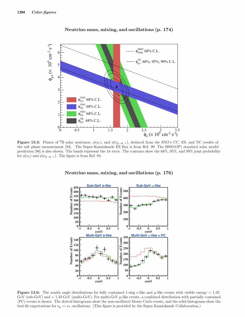
Figure 13.3: Fluxes of 8B solar neutrinos, φ(νe), and φ(νμ or τ ), deduced from the SNO’s CC, ES, and NC results ofthe salt phase measurement [94]. The Super-Kamiokande ES flux is from Ref. 99. The BS05(OP) standard solar modelprediction [86] is also shown. The bands represent the 1σ error. The contours show the 68%, 95%, and 99% joint probabilityfor φ(νe) and φ(νμ or τ ). The figure is from Ref. 94.


050

100150200250300350400450

-1 -0.5 0 0.5 1cosΘ

Num

ber

of E

vent

s

Sub-GeV e-like

0

100

200

300

400

500

-1 -0.5 0 0.5 1cosΘ

Num

ber

of E

vent

s

Sub-GeV μ-like

0

20

40

60

80

100

120

140

-1 -0.5 0 0.5 1cosΘ

Num

ber

of E

vent

s

Multi-GeV e-like

0

50

100

150

200

250

300

350

-1 -0.5 0 0.5 1cosΘ

Num

ber

of E

vent

s

Multi-GeV μ-like + PC

Figure 13.6: The zenith angle distributions for fully contained 1-ring e-like and μ-like events with visible energy < 1.33GeV (sub-GeV) and > 1.33 GeV (multi-GeV). For multi-GeV μ-like events, a combined distribution with partially contained(PC) events is shown. The dotted histograms show the non-oscillated Monte Carlo events, and the solid histograms show thebest-fit expectations for νμ ↔ ντ oscillations. (This figure is provided by the Super-Kamiokande Collaboration.)

Color figures 1395


Figure 13.10: The regions of squared-mass splitting and mixing angle favored or excluded by various experiments. Thefigure was contributed by H. Murayama (University of California, Berkeley, and IPMU, University of Tokyo). References tothe data used in the figure can be found at http://hitoshi.berkeley.edu/neutrino.

1396 Color figures


1e-05 0.0001 0.001 0.01 0.1 1

mMIN

[eV]

0.001

0.01

0.1

1

|<m

>| [e

V]

NH

IH

QD

Figure 13.11: The effective Majorana mass |<m>| (including a 2σ uncertainty) as a function of min(mj). The figure is

obtained using the best fit values and 1σ errors of Δm221, sin2 θ12, and |Δm2

31|∼= |Δm2

32| from Ref. 112, fixed sin2 θ13 = 0.01and δ = 0. The phases α21,31 are varied in the interval [0,π]. The predictions for the NH, IH and QD spectra areindicated. The black lines determine the ranges of values of |<m>| for the different pairs of CP conserving values of α21,31:(α21, α31)=(0, 0) solid, (0, π) long dashed, (π, 0) dash-dotted, (π, π) short dashed, lines. The red regions correspond to atleast one of the phases α21,31 and (α31 − α21) having a CP violating value. (Update by S. Pascoli of a figure from the lastarticle quoted in Ref. 127.)

Structure functions (p. 204)

0

0.2

0.4

0.6

0.8

1

1.2

10-4

10-3

10-2

10-1

x

x f(

x)

0

0.2

0.4

0.6

0.8

1

1.2

10-4

10-3

10-2

10-1

x

x f(

x)

Figure 16.4: Distributions of x times the unpolarized parton distributions f(x) (where f = uv, dv, u, d, s, c, b, g) and theirassociated uncertainties using the NNLO MSTW2008 parameterization [13] at a scale μ2 = 10 GeV2 and μ2 = 10, 000 GeV2.

Color figures 1397

Big-Bang cosmology (p. 233)

WMAP

SNLS

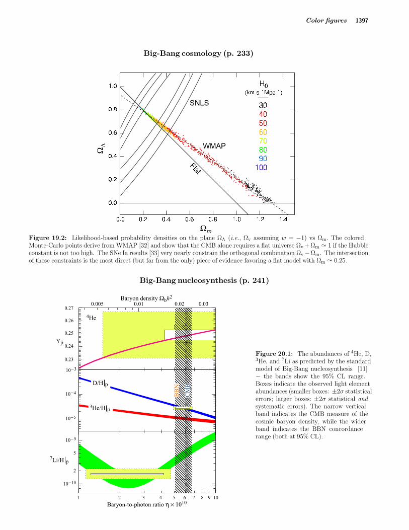
Figure 19.2: Likelihood-based probability densities on the plane ΩΛ (i.e., Ωv assuming w = −1) vs Ωm. The coloredMonte-Carlo points derive from WMAP [32] and show that the CMB alone requires a flat universe Ωv +Ωm � 1 if the Hubbleconstant is not too high. The SNe Ia results [33] very nearly constrain the orthogonal combination Ωv−Ωm. The intersectionof these constraints is the most direct (but far from the only) piece of evidence favoring a flat model with Ωm � 0.25.

Big-Bang nucleosynthesis (p. 241)

3He/H p

4He

2 3 4 5 6 7 8 9 101

0.01 0.02 0.030.005

CM

B

BB

N

Baryon-to-photon ratio η × 1010

Baryon density Ωbh2

D___H

0.24

0.23

0.25

0.26

0.27

10−4

10−3

10−5

10−9

10−10

2

57Li/H p

Yp

D/H p

Figure 20.1: The abundances of 4He, D,3He, and 7Li as predicted by the standardmodel of Big-Bang nucleosynthesis [11]− the bands show the 95% CL range.Boxes indicate the observed light elementabundances (smaller boxes: ±2σ statisticalerrors; larger boxes: ±2σ statistical and

systematic errors). The narrow verticalband indicates the CMB measure of thecosmic baryon density, while the widerband indicates the BBN concordancerange (both at 95% CL).

1398 Color figures

Cosmic microwave background (p. 264)

Figure 23.2: Band-power estimates from the WMAP, BOOMERANG, QUAD, CBI, and ACBAR experiments. Some ofthe low- and high- band-powers which have large error bars have been omitted. Note also that the widths of the -bandsvaries between experiments and have not been plotted. This figure represent only a selection of available experimentalresults, with some other data-sets being of similar quality. The multipole axis here is linear, so the Sachs-Wolfe plateau ishard to see. However, the acoustic peaks and damping region are very clearly observed, with no need for a theoretical curveto guide the eye; the curve plotted is a best-fit model from WMAP 5-year plus other CMB data.


Figure 23.3: Cross power spectrum of the temperature anisotropies and E-mode polarization signal from WMAP [47],together with estimates from BOOMERANG, DASI, QUAD, CBI and BICEP, several of which extend to higher . Note thatthe widths of the bands have been suppressed for clarity, but that in some cases they are almost as wide as the features inthe power spectrum. Also note that the y-axis here is not multiplied by the additional , which helps to show both the largeand small angular scale features.

Color figures 1399


Figure 23.4: Power spectrum of E-mode polarization from several different experiments, plotted along with a theoreticalmodel which fits WMAP plus other CMB data.

Cosmic Rays (p. 269)

Figure 24.1: Major components of theprimary cosmic radiation from Refs. [1–12].The figure was created by P. Boyle andD. Muller.

1400 Color figures

Cosmic Rays (p. 273)

GrigorovJACEE

MGUTienShan

Tibet07Akeno

CASA/MIAHegra

Flys EyeAgasa

HiRes1HiRes2

Auger SDAuger hybrid

Kascade

E [eV]

E2

.7F

(E)

[GeV

1.7

m−2

s−1sr

−1]

Ankle

Knee

2nd Knee

104

105

103

1014 10151013 1016 1017 1018 1019 1020

Figure 24.8: The all-particle spectrum from air shower measurements. The shaded area shows the range of the the directcosmic ray spectrum measurements.

Particle detectors at accelerators (p. 323)

0 2 4 6 8 101 3 5 7 9

Depth (nuclear interaction lengths)

1

10

100

3

30

300

Sca

led

me

an

nu

mb

er

of

pa

rtic

les in

co

un

ter

CDHS: 15 GeV

30 GeV

50 GeV

75 GeV

100 GeV

140 GeV

Figure 28.23: Mean profiles of π+ (mostly) induced cascades in the CDHS neutrino detector [137].

Color figures 1401

Particle detectors for non-accelerator physics (p. 333)

Eν [GeV]

106 107 108 109 1010 1011 1012102 103 104 10510−10

10−9

10−8

10−7

10−4

10−3

10−6

10−5

Atmospheric neutrino model

Gamma-ray bursts

Waxman-Bahcall bound

Cosmogenic neutrino flux

AMANDA-II unfolded νμAMANDA II νμ × 3AMANDA II cascades prelim.

IceCube projected 1 year νμ × 3

Eν

dNν/

dEν

[G

eV

cm

−2 s

−1 s

r−1]

2

Figure 29.5: Measured atmospheric neutrino fluxes above 100 GeV are shown together with a few generic models forastrophysical neutrinos and some limits.

Radioactivity and radiation protection (p. 342)

10-8

10-7

10-6

10-5

10-4

10-3

10-2

10-12

10-10

10-8

10-6

10-4

10-2

100

E d

Φ/d

E (

cm

-2 p

er

prim

ary

)

Energy (GeV)

80cm concrete, electrons x 10080cm concrete, protons

40cm iron, electrons x 10040cm iron, protons

Figure 30.2: Neutron energy spectra calculated with the FLUKA code [6,7] from 25 GeV proton and electron beams ona thick copper target. Spectra are evaluated at 90◦ to the beam direction behind 80 cm of concrete or 40 cm of iron. Allspectra are normalized per beam particle. In addition, spectra for electron beam are multiplied by a factor of 100.

1402 Color figures


0.1

1

10

100

1000

0.1 1 10 100 1000 10000

dD

/ d

t (

nS

v /

h)

Cooling Time, tc (h)

Copper, gamma

24Na

44Sc

44mSc

46Sc

48Sc

48V

52Mn

52mMn

54Mn

56Mn

55Co

56Co

58Co

57Ni

60Cu

61Cu

12.4 cm

measurement

FLUKA - total

FLUKA - gamma24

Na44

Sc,44m

Sc,46

Sc,48

Sc48

V52

Mn,52m

Mn,54

Mn,56

Mn55

Co,56

Co,58

Co57

Ni60

Cu,61

Cu

Figure 30.5: Contribution of individual gamma-emitting nuclides to the total dose rate at 12.4 cm distance to an activatedcopper sample [12].


0.1

1

10

100

1000

0.1 1 10 100 1000 10000

dD

/ d

t (

nS

v /

h)

Cooling Time, tc (h)

Copper, beta+

43Sc

44Sc

48V

52Mn

55Co

58Co

57Ni

61Cu

62Cu

64Cu

45Ti

12.4 cm

measurement

FLUKA - total

FLUKA - beta+43

Sc,44

Sc48

V52

Mn55

Co,58

Co57

Ni61

Cu,62

Cu,64

Cu45

Ti

Figure 30.6: Contribution of individual positron-emitting nuclides to the total dose rate at 12.4 cm distance to an activatedcopper sample [12].

Color figures 1403

Jet Production in pp and pp Interactions (p. 385)

(GeV)TE10 210

)(n

b/G

eV)

ηdT

/(d

Eσ2 d

-810

-710

-610

-510

-410

-310

-210

-110

1

10

210

310

|<0.7, η at 1.96 TeV, 0.1<| pCDF (p

|<0.7,η at 1.96 TeV,0.1<| pCDF (p

|<0.4)η at 1.96 TeV,0<| pD0 (p

|<0.7)η at 1.8 TeV,0.1<| pCDF (p

|<0.7)η at 1.8 TeV,0.1<| pD0 (p

|<0.5)η at 630 GeV, | pD0 (p

|<0.7)η at 546 GeV,0.1<| pCDF (p

|<0.85)η at 630 GeV, | pUA2 (p

|<0.7)η at 630 GeV, | UA1 (p

|=0)ηR807 (pp at 45 GeV, |

|=0)ηR807 (pp at 63 GeV, |

p

Midpoint algorithm)

algorithm)Tk

Figure 41.1: Inclusive differential jetcross sections plotted as a function of thejet tranverse energy. The CDF and D0measurements use a cone algorithm ofradius 0.7 for all results shown except forthe CDF measurements at 1.96 TeV whichalso use kT with a D parameter of 0.7 andmidpoint algorithms. The cone/kT resultsshould be similar if Rcone = D. UA1(UA2) uses a non-iterative cone algorithmwith a radius of 1.0 (1.3). Recent NLOQCD predictions (such as CTEQ6M)provide a good description of the CDF andD0 jet cross sections, Rept. on Prog. inPhys. 70, 89 (2007). Comparisons with theolder cross sections are more difficult dueto the nature of the jet algorithms used.CDF: Phys. Rev. D75, 092006 (2007),Phys. Rev. D64, 032001 (2001), Phys.Rev. Lett. 70, 1376 (1993); D0: Phys.Rev. D64, 032003 (2001); UA2: Phys.Lett. B257, 232 (1991); UA1: Phys. Lett.B172, 461 (1986); R807: Phys. Lett.B123, 133 (1983). (Courtesy of J. Huston,Michigan State University, 2010)

Direct γ Production in pp Interactions (p. 385)

(GeV/c)T

p10 210

)2(p

b/G

eV3

/dp

σ3E

d

-710

-610

-510

-410

-310

-210

-110

1

10

210

310

|<0.9)η at 1.96 TeV,| pD0 (p|<0.9)η at 1.8 TeV,| pCDF (p

|<0.9)η at 1.8 TeV,| pD0 (p|<2.5)η at 1.8 TeV,1.6<| pD0 (p

|<0.9)η at 630 GeV,| pD0 (p|<2.5)η at 630 GeV,1.6<| pD0 (p

|<0.9)η at 630 GeV,| pCDF (p=0)η at 630 GeV TeV, pUA2 (p=0)η at 630 GeV TeV, pUA1 (p

at 24.3 GeV TeV,<y>=0.4)pUA6 (p

Figure 41.2: Isolated photon crosssections plotted as a function of the photontransverse momentum. The errors areeither statistical only (CDF, D0 (1.96TeV), UA1, UA2, UA6) or uncorrelated(D0 1.8 TeV, 630 GeV). The data aregenerally in good agreement with NLOQCD predictions, albeit with a tendencyfor the data to be above (below) the theoryfor lower (large) transverse momenta,Phys. Rev. D59, 074007 (1999). D0:Phys. Lett. B639, 151 (2006), Phys. Rev.Lett. 87, 251805 (2001); CDF: Phys.Rev. D65, 112003 (2002); UA6: Phys.Lett. B206, 163 (1988); UA1: Phys.Lett. B209, 385 (1988); UA2: Phys. Lett.B288, 386 (1992). (Courtesy of J. Huston,Michigan State University, 2007)

1404 Color figures

Plots of cross sections and related quantities (p. 390)

σ and R in e+e− Collisions

10-8

10-7

10-6

10-5

10-4

10-3

10-2

1 10 102

σ[m

b]

ω

ρ

φ

ρ′

J/ψ

ψ(2S)Υ

Z

10-1

1

10

10 2

10 3

1 10 102

Rω

ρ

φ

ρ′

J/ψ ψ(2S)

Υ

Z

√s [GeV]

Figure 41.6: World data on the total cross section of e+e− → hadrons and the ratio R(s) = σ(e+e− →hadrons, s)/σ(e+e− → μ+μ−, s). σ(e+e− → hadrons, s) is the experimental cross section corrected for initial stateradiation and electron-positron vertex loops, σ(e+e− → μ+μ−, s) = 4πα2(s)/3s. Data errors are total below 2 GeV andstatistical above 2 GeV. The curves are an educative guide: the broken one (green) is a naive quark-parton model prediction,and the solid one (red) is 3-loop pQCD prediction (see “Quantum Chromodynamics” section of this Review, Eq. (9.7) or,for more details, K. G. Chetyrkin et al., Nucl. Phys. B586, 56 (2000) (Erratum ibid. B634, 413 (2002)). Breit-Wignerparameterizations of J/ψ, ψ(2S), and Υ(nS), n = 1, 2, 3, 4 are also shown. The full list of references to the original data andthe details of the R ratio extraction from them can be found in [arXiv:hep-ph/0312114]. Corresponding computer-readabledata files are available at http://pdg.lbl.gov/current/xsect/. (Courtesy of the COMPAS (Protvino) and HEPDATA(Durham) Groups, May 2010.)

Color figures 1405


R in Light-Flavor, Charm, and Beauty Threshold Regions

10-1

1

10

10 2

0.5 1 1.5 2 2.5 3

Sum of exclusivemeasurements

Inclusivemeasurements

3 loop pQCD

Naive quark model

u, d, s

ρ

ω

φ

ρ′

2

3

4

5

6

7

3 3.5 4 4.5 5

Mark-I

Mark-I + LGW

Mark-II

PLUTO

DASP

Crystal Ball

BES

J/ψ ψ(2S)

ψ3770

ψ4040

ψ4160

ψ4415

c

2

3

4

5

6

7

8

9.5 10 10.5 11

MD-1ARGUS CLEO CUSB DHHM

Crystal Ball CLEO II DASP LENA

Υ(1S)Υ(2S)

Υ(3S)

Υ(4S)

b

R

√s [GeV]

Figure 41.7: R in the light-flavor, charm, and beauty threshold regions. Data errors are total below 2 GeV and statisticalabove 2 GeV. The curves are the same as in Fig. 41.6. Note: CLEO data above Υ(4S) were not fully corrected for radiativeeffects, and we retain them on the plot only for illustrative purposes with a normalization factor of 0.8. The full list ofreferences to the original data and the details of the R ratio extraction from them can be found in [arXiv:hep-ph/0312114].The computer-readable data are available at http://pdg.lbl.gov/current/xsect/. (Courtesy of the COMPAS (Protvino)and HEPDATA (Durham) Groups, May 2010.)

1406 Color figures


10-4

10-3

10-2

10-1

1

10

10 2

1 10 102

103

104

➚➘⇓

⇓

⇓

To

tal

cro

ss s

ecti

on

(m

b)

⇓

104103102101.6

0.2

0.1

0.0

-0.1

-0.2

⇓

104103102101.6

⇓

104103102101.6

p−(p)p Σ−p

K∓p

π∓p

γp

γγ

p−p π−p

K−p

√sGeV

√sGeV

√sGeV

√sGeV

ppπ+p K+p

Re (T )Im (T )

Figure 41.10: Summary of hadronic, γp, and γγ total cross sections, and ratio of the real to imaginary parts of the forwardhadronic amplitudes. Corresponding computer-readable data files may be found at http://pdg.lbl.gov/current/xsect/.(Courtesy of the COMPAS group, IHEP, Protvino, August 2005)

Color figures 1407

The Mass and Width of the W boson (p. 418)

0

0.25

0.5

0.75

1

80 80.2 80.4 80.6 80.8 81

Entries 0

80.0 81.0

MW

[GeV]

ALEPH 80.440±0.051

DELPHI 80.336±0.067

L3 80.270±0.055

OPAL 80.416±0.053

LEP2 preliminary 80.376±0.033χ2

/dof = 49 / 41

CDF 80.421±0.043

D∅ 80.419±0.039

Tevatron [Run-1/2] 80.420±0.031χ2

/dof = 2.7 / 5

Overall average 80.399±0.023

Figure 1: Measurements of the W -boson mass by the LEP and Tevatron experiments.

The Mass and Width of the W boson (p. 419)

0

0.25

0.5

0.75

1

1.61.8 2 2.22.4

Entries 0

1.5 2.0 2.5

ΓW

[GeV]

ALEPH 2.14±0.11

DELPHI 2.39±0.17

L3 2.24±0.15

OPAL 2.00±0.14

LEP2 preliminary 2.196±0.083χ2

/dof = 37 / 33

CDF 2.033±0.064

D∅ 2.061±0.068

Tevatron [Run-1/2] 2.046±0.049χ2

/dof = 1.4 / 4

2.085±0.042

Figure 2: Measurements of the W -boson width by the LEP and Tevatron experiments.

1408 Color figures

Searches for Higgs Bosons (p. 450)

1

10

102

103

100 120 140 160 180 200

qq → WH

qq → ZH

gg → H

bb → H

gg,qq → ttH

qq → qqH

mH

[GeV]

σ [fb]

SM Higgs production

TeV II

TeV4LHC Higgs working group

Figure 1: SM Higgs boson production cross sections for pp collisions at 1.96 TeV, from Ref. [29] and references therein.


102

103

104

105

100 200 300 400 500

qq → WH

qq → ZH

gg → H

bb → H

qb → qtH

gg,qq → ttH

qq → qqH

mH

[GeV]

σ [fb]

SM Higgs production

LHC

TeV4LHC Higgs working group

Figure 2: SM Higgs boson production cross sections for pp collisions at 14 TeV [29].

Color figures 1409


10-2

10-1

1

20 40 60 80 100 120

mH(GeV/c2)

95%

CL

lim

it o

n ξ2

LEP√s = 91-210 GeV

ObservedExpected for background

Figure 5: The 95% confidence level upper bound on the ratio ξ2 = (gHZZ/gSMHZZ)2 [17]. The solid line indicates the observed

limit, and the dashed line indicates the median limit expected in the absence of a Higgs boson signal. The dark and lightshaded bands around the expected limit line correspond to the 68% and 95% probability bands, indicating the range ofstatistical fluctuations of the expected outcomes. The horizontal line corresponds to the Standard Model coupling. StandardModel Higgs boson decay branching fractions are assumed.


0

1

2

3

4

5

100 105 110 115 120 125 130 135 140 145 1500

1

2

3

4

5

mH(GeV/c

2)

95%

CL

Lim

it/S

M

Tevatron Run II Preliminary, L=2.0-5.4 fb-1

ExpectedObserved

±1σ Expected±2σ ExpectedLEP Exclusion

SM=1

November 6, 2009

Figure 6: Upper bound on the SM Higgs boson cross section obtained by combining CDF and DØ search results, as afunction of the mass of the Higgs boson sought [78]. The limits are shown as a multiple of the SM cross section. The ratiosof the different production and decay modes are assumed to be as predicted by the SM. The solid curve is the observed upperbound, and the dashed black curve is the median expected upper bound assuming no signal is present. The shaded bandsshow the 68% and 95% probability bands around the expected upper bound.

1410 Color figures


1

10

130 140 150 160 170 180 190 200

1

10

mH

(GeV)

Rli

mCDF + D0 Run IIL=4.8-5.4 fb

-1Expected

Observed

Expected ±1σExpected ±2σ

SM=1

Figure 7: Upper bound on the SM Higgs boson cross section obtained by combining CDF and DØ search results in theH → W+W− decay mode, as a function of the mass of the Higgs boson sought [19]. The limits are shown as a multiple ofthe SM cross section. The ratios of the different production and decay modes are assumed to be as predicted by the SM. Thesolid curve shows the observed upper bound, the dashed black curve shows the median expected upper bound assuming nosignal is present. The shaded bands show the 68% and 95% probability bands around the expected upper bound.


0

1

2

3

4

5

6

120 140 160 180 200 220 240 260 280 3000

1

2

3

4

5

6

mH

(GeV)

95%

C.L

. L

imit

/4G

(low

Mass

) P

redic

tion

CDF+D0 Run II

L=4.8 - 5.4 fb-1

4G(Low Mass)=1

Expected

Observed

±1 s.d. Expected

±2 s.d. Expected

4G(High Mass)

Figure 8: Upper bound on the Higgs boson cross section of the 4th generation sequential model obtained by combiningCDF and DØ search results in the H →W+W− decay mode, as a function of the mass of the Higgs boson sought [87]. Thelimits are shown as a multiple of the cross section obtained in this extended model. The solid curve shows the observed upperbound, the dashed black curve shows the median expected upper bound assuming no signal is present, and the colored bandsshow the 68% and 95% probability bands around the expected upper bound.

Color figures 1411


1

10

0 20 40 60 80 100 120 140

1

10

mh (GeV/c

2)

tanβ

Excludedby LEP

TheoreticallyInaccessible

mh-max

Figure 9: The MSSM exclusion contours, at 95% C.L. (light-green) and 99.7% CL (dark-green), obtained by LEP for theCPC mh-max benchmark scenario, with mt = 174.3 GeV. The figure shows the excluded and theoretically inaccessibleregions in the (mh, tanβ) projection. The upper edge of the theoretically allowed region is sensitive to the top quark mass; itis indicated, from left to right, for mt = 169.3, 174.3, 179.3 and 183.0 GeV. The dashed lines indicate the boundaries of theregions which are expected to be excluded on the basis of Monte Carlo simulations with no signal (from Ref. [18]) .


1

10

102

103

100 125 150 175 200 225 250 275 300

mφ (GeV/c2)

95%

C.L

. L

imit

on σ

×BR

(pb)

Tevatron Run II Preliminary

CDF bbb Obs. Limit 2.5 fb-1

CDF bbb Exp. Limit

D∅ bbb Obs. Limit 2.6 fb-1

D∅ bbb Exp. Limit

D∅ ττ Obs. Limit 2.2 fb-1

D∅ ττ Exp. Limit

CDF ττ Obs. Limit 1.8 fb-1

CDF ττ Exp. Limit

CDF+D∅ ττ Obs. Limit

CDF+D∅ ττ Exp. Limit

D∅ bττ Obs. Limit

D∅ bττ Exp. Limit

Figure 10: The 95% C.L. limits on σ(bb̄φ) × BR(φ → bb̄) and σ(φ + X) × BR(φ → τ+τ−) from the Tevatron collaborations. The DØ limit on σ(bb̄φ)×BR(φ→ τ+τ−) and the Tevatron combined limit on σ(φ + X)×BR(φ→ τ+τ−) are alsoshown. The observed limits are indicated with solid lines, and the expected limits are indicated with dashed lines. The limitsare to be compared with the sum of signal predictions for Higgs bosons with similar masses. The decay widths of the Higgsbosons are assumed to be much smaller than the experimental resolution.

1412 Color figures


]2 [GeV/cAm

100 120 140 160 180 200

βta

n

10

20

30

40

50

60

70

80

90

100

Excluded by LEP

Observed limit

Expected limit

σ 1 ±Expected limit


=+200 GeVμ max, hm

-1Tevatron Run II Preliminary, L= 1.8-2.2 fb

]2 [GeV/cAm

100 120 140 160 180 200

βta

n

10

20

30

40

50

60

70

80

90

100

]2 [GeV/cAm

100 120 140 160 180 200

βta

n

10

20

30

40

50

60

70

80

90

100

Excluded by LEP

Observed limit

Expected limit



=+200 GeVμno mixing,

-1Tevatron Run II Preliminary, L= 1.8-2.2 fb

]2 [GeV/cAm

100 120 140 160 180 200

βta

n

10

20

30

40

50

60

70

80

90

100

Figure 11: The 95% C.L. MSSM exclusion contours obtained by a combination of the CDF and DØ searches for H → τ+τ−

in the mh-max (left) and no-mixing (right) benchmark scenarios, both with μ = 200 GeV, projected onto the (mA, tanβ)plane [147]. The regions above the solid black line are excluded, and the shaded and hatched bands centered on the lighterline show the dis tributions of expected exclusions in the absence of a signal. Also shown are the regions excluded by LEPsearches [18], assuming a top quark mass of 174.3 GeV. The Tevatron results are not sensitive to the precise value of the topquark mass.


1

10

0 20 40 60 80 100 120 140

1

10

mH1

(GeV/c2)

tanβ

Excludedby LEP

TheoreticallyInaccessibleCPX

Figure 12: The MSSM exclusion contours, at the 95% C.L. (light-green) and the 99.7% CL (dark-green), obtained by LEPfor the CPX scenario defined in the text. Here, mt = 174.3 GeV. The figure shows the excluded and theoretically inaccessibleregions in the (mH1

, tanβ) projection. The dashed lines indicate the boundary of the region which is expected to be excludedat the 95% C.L. in the absence of a signal.

Color figures 1413


βtan10

-11 10 10

2

)2

c (

GeV

/±

Hm

60

80

100

120

140

160

60

80

100

120

140

160

LEP (ALEPH, DELPHI, L3 and OPAL)

onlys c→± or Hντ→±

Assuming H

Th

eo

reti

ca

lly

ina

cc

es

sib

le

Th

eo

reti

ca

lly

ina

cc

es

sib

le

Expected Limit

Expectedσ 1 ±SM

CDF Run II Excluded

LEP Excluded

Expected Limit

Expected Limitσ 1 ±CDF Run II Excluded

LEP Excluded

Figure 13: Summary of the 95% C.L. exclusions in the (mH+, tan β) plane obtained by LEP [195] and CDF [214]. Thebenchmark scenario parameters used to interpret the CDF results are very close to those of the mmax

h scenario, and mt isassumed to be 175 GeV. The full lines indicate the median limits expected in the absence of a H± signal, and the horizontalhatching represents the ±1σ bands about this expectation.


Figure 14: The 95% C.L. exclusion limits on the masses and couplings to leptons of right- and left-handed doubly-chargedHiggs bosons, obtained by LEP and Tevatron experiments (from Ref. [223]) .

1414 Color figures

W ′-boson searches (p. 481)

W’ Mass (GeV)300 400 500 600 700 800 900

SM

g’

/ g

0

0.2

0.4

0.6

0.8

1

1.2

Excluded Region

)νObserved Limit for M(W’) < M(

)νObserved Limit for M(W’) > M(

Standard Model

-195% C.L. Limit on Coupling - CDF Run II Preliminary: 955 pb

Figure 1: 95% CL exclusion limit from CDF [17] in the gauge coupling versus MW ′ plane, using the tb̄ and t̄b final states.

Leptoquarks (p. 491)

Figure 1: Limits on two typical first-generation scalar leptoquark states in the mass-coupling plane. The upper figure isfor a weak-isodoublet, weak-hypercharge 7/6, 3B + L = 0 leptoquark state, while the lower figure for a weak-isosinglet,weak-hypercharge −1/3, 3B + L = 2 state.

Color figures 1415

CP Violation in KL Decays (p. 780)

0.515

φ + _

(degre

es)

mKL - mKS (1010

hs-1)

0.520 0.525 0.530 0.535 0.54038

40

42

44

46

48

c ed

ba

g f

c

d

e

f

j

Figure 1: φ+− vs Δm for experiments which do not assume CPT invariance. Δm measurements appear as vertical bandsspanning Δm± 1σ, cut near the top and bottom to aid the eye. Most φ+− measurements appear as diagonal bands spanningφ+− ± σφ. Data are labeled by letters: “b”–FNAL KTeV, “c”–CERN CPLEAR, “d”–FNAL E773, “e”–FNAL E731,

“f”–CERN, “g”–CERN NA31, and are cited in Table 1. The narrow band “j” shows φSW. The ellipse “a” shows the χ2 = 1contour of the fit result.

CP Violation in KL Decays (p. 781)

φ + _

(degre

es)

38

40

42

44

46

48

0.888

τKs (10-10

s)

0.892 0.896 0.900 0.904

hi

g

f

c

d

e

a

b

j

Figure 2: φ+− vs τS. τ

Smeasurements appear as vertical bands spanning τ

S± 1σ, some of which are cut near the top and

bottom to aid the eye. Most φ+− measurements appear as diagonal or horizontal bands spanning φ+−±σφ. Data are labeledby letters: “b”–FNAL KTeV, “c”–CERN CPLEAR, “d”–FNAL E773, “e”–FNAL E731, “f”–CERN, “g”–CERN NA31,“h”–CERN NA48, “i”–CERN NA31, and are cited in Table 1. The narrow band “j” shows φSW. The ellipse “a” shows thefit result’s χ2 = 1 contour.

1416 Color figures

D0–D0 Mixing (p. 825)

Figure 1: Two-dimensional 1σ-5σ contours for (x, y) from measurements of D0 → K(∗)+ ν, h+h−, K+π−, K+π−π0,K+π−π+π−, K0

Sπ+π−, and K0SK+K− decays, and double-tagged branching fractions measured at the ψ(3770) resonance

(from HFAG [10]) .

D0–D0 Mixing (p. 825)

Figure 2: Two-dimensional 1σ-5σ contours for (|q/p|,Arg(q/p)) from measurements of D0 → K(∗)+ ν, h+h−, K+π−,K+π−π0, K+π−π+π−, K0

Sπ+π−, and K0SK+K− decays, and double-tagged branching fractions measured at the ψ(3770)

resonance (from HFAG [10]) .

Color figures 1417

B0–B0 Mixing (p. 976)

–1

0

1

2

–1

0

1

2

–1

0

1

2

0 5 10 15 20 25 30

Bs o

scill

atio

n am

plit

ude

data ± 1 σ1.645 σ

sensitivity 31.0 ps–1

data ± 1.645 σdata ± 1.645 σ (stat only)

CDF2 observation (2006)April 2010

data ± 1 σ1.645 σ



D0 evidence (2007, preliminary)

Δms (ps–1)

data ± 1 σ

95% CL limit 14.6 ps–1

1.645 σ



Average of all others (1997–2004)

Δms = 17.77 ± 0.10 ± 0.07 ps–1

Δms = 18.53 ± 0.93 ± 0.30 ps–1

Figure 2: Combined measurements of the B0s oscillation amplitude as a function of Δms. Top: CDF result based on Run

II data, published in 2006 [19]. Middle: Average of all preliminary DØ results available at the end of 2007 [21]. Bottom:Average of all other results (mainly from LEP and SLD) published between 1997 and 2004. All measurements are dominatedby statistical uncertainties. Neighboring points are statistically correlated.

1418 Color figures

Vcb and Vub CKM Matrix Elements (p. 1016)

2ρ0 0.5 1 1.5 2

]-3

| [1

0cb

|V

×F

(1)

30

35

40

45

HFAGLP 2009

ALEPH

CLEO

OPAL(part. reco.)

OPAL(excl.)

DELPHI(part. reco.)

BELLE

DELPHI(excl.)

BABAR (excl.)

BABAR (D*0)

BABAR (Global Fit)

AVERAGE

= 12χΔ

/dof = 56.9/212χ

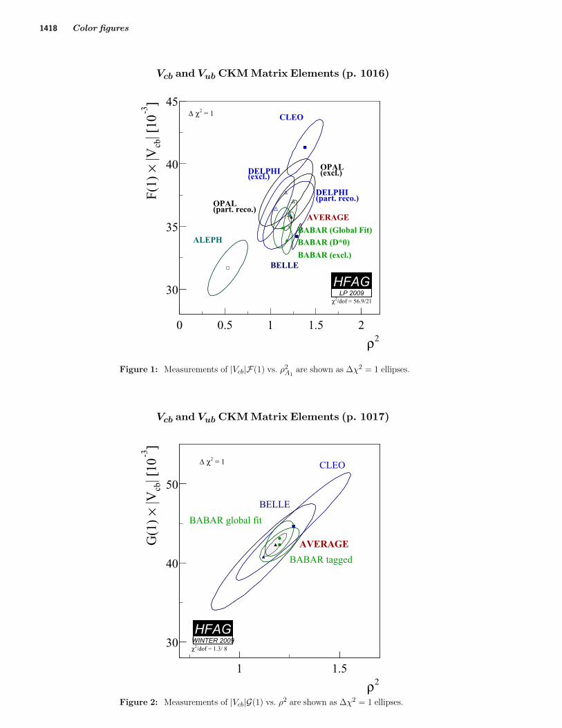
Figure 1: Measurements of |Vcb|F(1) vs. ρ2A1

are shown as Δχ2 = 1 ellipses.

Vcb and Vub CKM Matrix Elements (p. 1017)

2ρ1 1.5

]-3

| [1

0cb

|V

×G

(1)

30

40

50

HFAGWINTER 2009

CLEO

BELLE

BABAR global fit

BABAR tagged

AVERAGE

= 12χΔ

/dof = 1.3/ 82χ

Figure 2: Measurements of |Vcb|G(1) vs. ρ2 are shown as Δχ2 = 1 ellipses.

Color figures 1419

Supersymmetry, Part I (Theory) (p. 1301)

0

100

200

300

400

500

600

700

m [GeV]mSUGRA SPS 1a′/SPA

l̃R

l̃Lν̃l

τ̃1

τ̃2ν̃τ

χ̃01

χ̃02

χ̃03

χ̃04

χ̃±1

χ̃±2

q̃R

q̃L

g̃

t̃1

t̃2

b̃1

b̃2

h0

H0, A0 H±

Figure 1: Mass spectrum of supersymmetric particles and Higgs bosons for the mSUGRA reference point SPS 1a′. The

masses of the first and second generation squarks, sleptons, and sneutrinos are denoted collectively by q̃, ̃ and ν̃�, respectively.Taken from Ref. 100.

Supersymmetry, Part II (Experiment) (p. 1311)

0

20

40

60

80

100

50 60 70 80 90 100Mμ (GeV/c

2)

Mχ

(GeV

/c2)

˜

μ̃ μ̃R R

+ -

(*): B(χ1μ)=1

(*)

√s = 183-208 GeV

ADLO

Excluded at 95% CL

(μ=-200 GeV, tanβ=1.5)

Observed

Expected

Figure 1: Region in the (mμ̃R, mχ̃0

1) plane excluded by the searches for smuons at LEP.

1420 Color figures


)2

(GeV/cg~M

0 100 200 300 400 500 600

)2 (

GeV

/cq~

M

0

100

200

300

400

500

600

no mSUGRA

solution

LEP

UA

1

UA

2

g~

= M

q~M

)2

(GeV/cg~M

0 100 200 300 400 500 600

)2 (

GeV

/cq~

M

0

100

200

300

400

500

600observed limit 95% C.L.

expected limit

FNAL Run I

LEP II

<0μ=5,β=0, tan0A-1L = 2.0 fb

Figure 3: Region in the (mg̃, mq̃) plane excluded by CDF Run II and by earlier experiments.


(GeV)0

m0 50 100 150 200 250

(G

eV

)1/2

m

150

200

250

300

(GeV)0

m0 50 100 150 200 250

(G

eV

)1/2

m

150

200

250

300DØ observed limitDØ expected limit

CDF observed)-1limit (2.0 fb

LEP Chargino Limit

LEPSleptonLimit

-1DØ, 2.3 fbmSUGRA

> 0μ = 0, 0

= 3, Aβtan

2

0χ∼1

±χ∼Search for

)2

0χ∼

M(

≈)l~M

(

)1

±χ∼

M(

≈)ν∼

M(

(GeV)0

m0 50 100 150 200 250

(G

eV

)1/2

m

150

200

250

300

Figure 6: Regions in the (m0,m1/2) plane excluded by the DØ search for trileptons and by the LEP experiments.

Color figures 1421

Dynamical Electroweak Symmetry Breaking (p. 1341)

) (GeV)T

ρM(160 180 200 220

) (G

eV

)Tπ

M(

60

80

100

120

(a)

= 500 GeVVM

-1DØ, 388 pb

pro

duction th

reshold

TπW

production th

reshold

TπTπ

Expected Exclusion (NN)

Expected Exclusion (Cut-based)

) (GeV)T

ρM(160 180 200 220

) (G

eV

)Tπ

M(

60

80

100

120

(b)

= 500 GeVVM

-1DØ, 388 pb

pro

duction th

reshold

TπW

production th

reshold

TπTπ

Excluded Region (NN)

Excluded Region (Cut-based)

Figure 1: Search for a light technirho decaying to W± and a πT , and in which the πT decays to two jets including at leastone b quark [19]. Expected region of exclusion (a) and excluded region (b) at the 95% C.L. in the M(ρT ), M(πT ) planefor ρT → WπT → eν bb̄(c̄) production with MV = 500 GeV. Kinematic thresholds from WπT and πTπT are shown on thefigures.

1422 Color figures


DELPHI

60

80

100

120

100 200 300 400

e+e

-→πTπ

T;π

TW

L

e+e

-→ρT(γ) :

ρT→hadrons

ρT→W

+LW

-L

ND=9

M(ρT) [GeV/c

2]

M(π

T)

[GeV

/c2]

Figure 4: 95% CL exclusion region [23] in the technirho-technipion mass plane obtained from searches by the DELPHIcollaboration at LEP 2, for nine technifermion doublets. The dashed line shows the expected limit for the 4-jet analysis.


Figure 6: 95% CL exclusion region [28] in the technirho-technipion mass plane for pair produced technipions, withleptoquark couplings, decaying to bν.

color figures -...

Documents