collocation methods for nonlinear parabolic partial differential equations · 2017-04-28 ·...
TRANSCRIPT
Collocation Methods for Nonlinear Parabolic Partial
Differential Equations
Xu Chen
A Thesis
in
The Department
of
Computer Science
Presented in Partial Fulfillment of the Requirements
for the Degree of
Master of Computer Science at
Concordia University
Montreal, Quebec, Canada
April 2017
c© Xu Chen, 2017

CONCORDIA UNIVERSITY
School of Graduate Studies
This is to certify that the thesis prepared
By: Xu Chen
Entitled: Collocation Methods for Nonlinear Parabolic Partial Differential
Equations
and submitted in partial fulfillment of the requirements for the degree of
Master of Computer Science
complies with the regulations of this University and meets the accepted standards with respect to
originality and quality.
Signed by the Final Examining Committee:
ChairDr. Name of the Chair
ExaminerDr. Tien D. Bui
ExaminerDr. Adam Krzyzak
SupervisorDr. Eusebius Doedel
Approved bySudhir Mudur, ChairDepartment of Computer Science
2017Dr. Amir Asif, DeanFaculty of Engineering and Computer Science

Abstract
Collocation Methods for Nonlinear Parabolic Partial Differential Equations
Xu Chen
In this thesis, we present an implementation of a novel collocation method for solving nonlin-
ear parabolic partial differential equations (PDEs) based on triangle meshes. The temporal partial
derivative is discretized using the implicit Euler-backward finite difference scheme. The spatial
domain of the PDEs discussed in this thesis is two-dimensional. The domain is first triangulated
and then refined into appropriately sized triangular elements by the Rivara algorithm. The solution
is approximated by piecewise polynomials in the elements. The polynomial in each element is re-
quired to satisfy the PDE at collocation points of the element and keep a certain degree of continuity
with the polynomials in the neighboring elements via matching points. Nested dissection is used
recursively, from the elements up to the entire domain, to merge all pairs of sibling sub-regions
for eliminating the variables at the matching points on the common sides shared by the merged
sub-regions. Then by applying global boundary conditions, we solve for the solution values at the
boundary points of the entire domain. The solutions at the boundary points of the domain are back-
substituted to solve the variables at the matching points of the sub-regions. This back-substitution
is repeated until every element is reached. The accuracy of the solution is affected by the time
step, granularity of the subdivision, the number and location of matching points, and the number
and location of collocation points. Increasing the number of matching points or collocation points
does not always improve the accuracy. Instead, it may cause singularity. We have given several
layouts of specific numbers of collocation and matching points which bring high accuracy. Our so-
lution visualization algorithm directly renders mathematical surfaces instead of any approximation
of them. Thus each pixel of the rendered surfaces exactly reflects the corresponding fragment on
the mathematical surfaces.
iii

Acknowledgments
I would like to express my sincere gratitude to my supervisor Dr. Eusebius J.Doedel, for his
continuous support of my project and thesis, for his patience, motivation, and guidance.
iv

Contents
List of Figures viii
List of Tables xii
1 Introduction 1
1.1 Partial differential equations . . . . . . . . . . . . . . . . . . . . . . . . . . . . . 1
1.2 Linear and nonlinear second order partial differential equations . . . . . . . . . . . 2
1.3 Nonlinear parabolic partial differential equations . . . . . . . . . . . . . . . . . . 2
1.4 Numerical methods . . . . . . . . . . . . . . . . . . . . . . . . . . . . . . . . . . 4
1.4.1 The finite difference method . . . . . . . . . . . . . . . . . . . . . . . . . 5
1.4.2 The finite element method . . . . . . . . . . . . . . . . . . . . . . . . . . 5
1.4.3 The collocation method . . . . . . . . . . . . . . . . . . . . . . . . . . . . 6
1.5 Organization of the thesis . . . . . . . . . . . . . . . . . . . . . . . . . . . . . . . 8
2 Mesh Generation 9
2.1 Local adaptive mesh refinement . . . . . . . . . . . . . . . . . . . . . . . . . . . 9
2.2 Triangulation of polygonal domains . . . . . . . . . . . . . . . . . . . . . . . . . 12
2.3 The Rivara algorithm . . . . . . . . . . . . . . . . . . . . . . . . . . . . . . . . . 13
2.4 3D mesh refinement . . . . . . . . . . . . . . . . . . . . . . . . . . . . . . . . . . 16
2.5 Other mesh generation methods . . . . . . . . . . . . . . . . . . . . . . . . . . . 18
3 A Collocation Method for Nonlinear Parabolic PDE BVP 19
3.1 Nonlinear parabolic PDE problems . . . . . . . . . . . . . . . . . . . . . . . . . . 19
v

3.2 Collocation with discontinuous piecewise polynomials . . . . . . . . . . . . . . . 21
3.3 Newton’s method . . . . . . . . . . . . . . . . . . . . . . . . . . . . . . . . . . . 24
3.4 The choice of basis polynomials . . . . . . . . . . . . . . . . . . . . . . . . . . . 32
3.5 The collocation method with initial and boundary conditions . . . . . . . . . . . . 33
4 Numerical Linear Algebra 35
4.1 The global linear system . . . . . . . . . . . . . . . . . . . . . . . . . . . . . . . 35
4.2 Nested dissection . . . . . . . . . . . . . . . . . . . . . . . . . . . . . . . . . . . 38
4.3 Generalization of the nested dissection . . . . . . . . . . . . . . . . . . . . . . . . 42
4.4 Complexity analysis . . . . . . . . . . . . . . . . . . . . . . . . . . . . . . . . . . 43
5 Implementation 46
5.1 Overview of the prototype implementation . . . . . . . . . . . . . . . . . . . . . . 47
5.2 Work flow for solving a PDE . . . . . . . . . . . . . . . . . . . . . . . . . . . . . 50
5.3 Data structure . . . . . . . . . . . . . . . . . . . . . . . . . . . . . . . . . . . . . 54
5.4 Optimization . . . . . . . . . . . . . . . . . . . . . . . . . . . . . . . . . . . . . 62
5.5 The Eigen library . . . . . . . . . . . . . . . . . . . . . . . . . . . . . . . . . . . 65
6 Numerical Results 67
6.1 Factors determining accuracy and convergence . . . . . . . . . . . . . . . . . . . 67
6.1.1 Mesh size . . . . . . . . . . . . . . . . . . . . . . . . . . . . . . . . . . . 67
6.1.2 The number of collocation points and matching points . . . . . . . . . . . 69
6.1.3 Location of collocation points and matching points . . . . . . . . . . . . . 71
6.1.4 Templates of collocation and matching points . . . . . . . . . . . . . . . . 71
6.2 Initial condition and time integration . . . . . . . . . . . . . . . . . . . . . . . . . 74
6.3 Example PDEs for numerical experiments . . . . . . . . . . . . . . . . . . . . . . 76
6.3.1 A linear parabolic PDE with a stationary solution . . . . . . . . . . . . . . 76
6.3.2 Another linear parabolic PDE with a stationary solution . . . . . . . . . . 83
6.3.3 A nonlinear parabolic PDE with a stationary solution . . . . . . . . . . . . 86
6.3.4 Another nonlinear parabolic PDE with a stationary solution . . . . . . . . 93
vi

6.3.5 A nonlinear parabolic PDE without stationary solution . . . . . . . . . . . 96
6.4 Application . . . . . . . . . . . . . . . . . . . . . . . . . . . . . . . . . . . . . . 99
6.4.1 The Gelfand-Bratu problem . . . . . . . . . . . . . . . . . . . . . . . . . 99
6.4.2 Numerical solution of the Gelfand-Bratu problem in 2D . . . . . . . . . . 100
6.5 Summary of numerical results . . . . . . . . . . . . . . . . . . . . . . . . . . . . 104
7 Visualization 106
7.1 Pixel-correct mathematical surface rendering . . . . . . . . . . . . . . . . . . . . 107
7.2 The principle of our rendering algorithm . . . . . . . . . . . . . . . . . . . . . . . 109
7.3 Technical details . . . . . . . . . . . . . . . . . . . . . . . . . . . . . . . . . . . 112
8 Conclusions and Discussion 116
Bibliography 118
Appendix A Code of Visualization Program 125
vii

List of Figures
Figure 1.1 A numerical solution of the Bratu problem in an irregularly shaped 2D do-
main by the finite element collocation method . . . . . . . . . . . . . . . . . . . . 7
Figure 2.1 A locally refined triangular mesh adapted to a 2D Gaussian function. . . . . 10
Figure 2.2 The profile of the 2D Gaussian function from [30] . . . . . . . . . . . . . . 10
Figure 2.3 A locally refined triangular mesh adapted to an ideal 2D low-pass filter . . . 10
Figure 2.4 The ideal 2D low-pass filter . . . . . . . . . . . . . . . . . . . . . . . . . . 10
Figure 2.5 Measuring how much a piecewise polynomial surface is bent . . . . . . . . 11
Figure 2.6 Shapes with large aspect ratios: (a) angle too large; (b) angle too small. . . . 14
Figure 2.7 (a) Generating a triangular mesh by triangulation. . . . . . . . . . . . . . . 14
Figure 2.8 (b) Refinement of the triangular mesh. . . . . . . . . . . . . . . . . . . . . 14
Figure 2.9 (a) Generating a triangular mesh by triangulation. . . . . . . . . . . . . . . 14
Figure 2.10 (b) Refinement of the triangular mesh. . . . . . . . . . . . . . . . . . . . . 14
Figure 2.11 A domain triangulated and refined at the first level. . . . . . . . . . . . . . 16
Figure 2.12 The domain after 2 levels of refinement: level 1 and 2. . . . . . . . . . . . . 16
Figure 3.1 A triangular mesh for the 2D collocation method. . . . . . . . . . . . . . . 23
Figure 3.2 Collocation and matching points of an element. . . . . . . . . . . . . . . . 23
Figure 3.3 4x3 matching points with 3 collocation points. . . . . . . . . . . . . . . . . 28
Figure 3.4 6x3 matching points with 10 collocation points. . . . . . . . . . . . . . . . 28
Figure 3.5 6x3 matching points with 10 relocated collocation points. . . . . . . . . . . 32
Figure 4.1 A domain composed of 4 elements. . . . . . . . . . . . . . . . . . . . . . . 36
Figure 4.2 Region Ωi, its pair of sibling sub-regions Ωi1 and Ωi2, and the boundaries. . 39
viii
Figure 4.3 A region bisected into a pair of equal subregions by a single straight line. . . 43
Figure 4.4 A region subdivided into a pair of irregularly-shaped and -sized subregions
by a polyline. . . . . . . . . . . . . . . . . . . . . . . . . . . . . . . . . . . . . . 43
Figure 4.5 A region subdivided into a pair of nested subregions by a closed polyline. . 43
Figure 4.6 A region subdivided into a pair of subregions by 2 separate polylines. . . . . 43
Figure 5.1 Software architect pattern of Model-View-Controller . . . . . . . . . . . . 48
Figure 5.2 View: 2D visualization of solutions . . . . . . . . . . . . . . . . . . . . . . 49
Figure 5.3 View: 3D visualization of solutions . . . . . . . . . . . . . . . . . . . . . . 49
Figure 5.4 Controller: parameters and selection of test PDEs . . . . . . . . . . . . . . 50
Figure 5.5 Work flow of the solver based on the collocation method . . . . . . . . . . 51
Figure 5.6 The subdivision tree . . . . . . . . . . . . . . . . . . . . . . . . . . . . . . 52
Figure 5.7 CSolver . . . . . . . . . . . . . . . . . . . . . . . . . . . . . . . . . . . . 54
Figure 5.8 Container CMesh contains all mesh information: vertices, edges, and elements. 55
Figure 5.9 CVertex and linked list of vertices. . . . . . . . . . . . . . . . . . . . . . . 56
Figure 5.10 CEdge and the linked list of edges. . . . . . . . . . . . . . . . . . . . . . . 56
Figure 5.11 CElement and the linked list of elements. . . . . . . . . . . . . . . . . . . . 58
Figure 5.12 CMergedRegion . . . . . . . . . . . . . . . . . . . . . . . . . . . . . . . . 59
Figure 5.13 Merging of elements and merged regions . . . . . . . . . . . . . . . . . . . 60
Figure 5.14 CSubMatrix and its data buffer. . . . . . . . . . . . . . . . . . . . . . . . . 61
Figure 5.15 CMergeInfo . . . . . . . . . . . . . . . . . . . . . . . . . . . . . . . . . . 62
Figure 5.16 Class Diagram 1 . . . . . . . . . . . . . . . . . . . . . . . . . . . . . . . . 63
Figure 5.17 Class Diagram 2 . . . . . . . . . . . . . . . . . . . . . . . . . . . . . . . . 64
Figure 6.1 4x3 matching points with 1 collocation point. . . . . . . . . . . . . . . . . 70
Figure 6.2 4x3 matching points with 2 collocation points. . . . . . . . . . . . . . . . . 70
Figure 6.3 6x3 matching points with 4 collocation points. . . . . . . . . . . . . . . . . 70
Figure 6.4 6x3 matching points with 7 collocation points. . . . . . . . . . . . . . . . . 70
Figure 6.5 Locations of Gauss points . . . . . . . . . . . . . . . . . . . . . . . . . . . 72
Figure 6.6 Location of collocation points in a triangular element . . . . . . . . . . . . 72
Figure 6.7 A copy of the TABLE I from [22]. . . . . . . . . . . . . . . . . . . . . . . 74
ix

Figure 6.8 Profile of F (x, y). . . . . . . . . . . . . . . . . . . . . . . . . . . . . . . . 75
Figure 6.9 The solution at t = 0.004, observed from below . . . . . . . . . . . . . . . 77
Figure 6.10 The solution at t = 0.008 . . . . . . . . . . . . . . . . . . . . . . . . . . . 77
Figure 6.11 The solution at t = 0.02 . . . . . . . . . . . . . . . . . . . . . . . . . . . . 77
Figure 6.12 The solution at t = 0.05 . . . . . . . . . . . . . . . . . . . . . . . . . . . . 77
Figure 6.13 Solution at t = 0.1 . . . . . . . . . . . . . . . . . . . . . . . . . . . . . . . 77
Figure 6.14 A near stationary solution when t � 3.0. . . . . . . . . . . . . . . . . . . . 77
Figure 6.15 The initial condition . . . . . . . . . . . . . . . . . . . . . . . . . . . . . . 78
Figure 6.16 The transient solution at t = 0.05 . . . . . . . . . . . . . . . . . . . . . . . 78
Figure 6.17 The transient solution at t = 0.1 . . . . . . . . . . . . . . . . . . . . . . . 78
Figure 6.18 The transient solution at t � 1.0 . . . . . . . . . . . . . . . . . . . . . . . 78
Figure 6.19 The stationary solution of PDE (6.8); center value ≈ 0.1699. . . . . . . . . 84
Figure 6.20 The stationary solution of PDE (6.8). . . . . . . . . . . . . . . . . . . . . . 84
Figure 6.21 The values of θ for various values of λ from [23] . . . . . . . . . . . . . . . 87
Figure 6.22 The values of u(0.5, 0.5) for various values of λ from [23] . . . . . . . . . 87
Figure 6.23 θ=3, λ=5.37, 3x3 matching points, 4 collocation points, 64 elements . . . . 91
Figure 6.24 θ=3, λ=5.37, 2x3 matching points, 1 collocation point, 64 elements . . . . . 91
Figure 6.25 θ=3, λ=5.37, 3x3 matching points, 4 collocation pointss, 256 elements . . . 91
Figure 6.26 θ=3, λ=5.37, 2x3 matching points, 1 collocation point, 1024 elements . . . 91
Figure 6.27 Solution families found by our collocation method . . . . . . . . . . . . . . 92
Figure 6.28 t = 0.01 . . . . . . . . . . . . . . . . . . . . . . . . . . . . . . . . . . . . 94
Figure 6.29 t = 0.02 . . . . . . . . . . . . . . . . . . . . . . . . . . . . . . . . . . . . 94
Figure 6.30 t = 0.03 . . . . . . . . . . . . . . . . . . . . . . . . . . . . . . . . . . . . 94
Figure 6.31 t = 0.04 . . . . . . . . . . . . . . . . . . . . . . . . . . . . . . . . . . . . 94
Figure 6.32 t = 0.06 . . . . . . . . . . . . . . . . . . . . . . . . . . . . . . . . . . . . 95
Figure 6.33 t = 0.07 . . . . . . . . . . . . . . . . . . . . . . . . . . . . . . . . . . . . 95
Figure 6.34 t = 0.08 . . . . . . . . . . . . . . . . . . . . . . . . . . . . . . . . . . . . 95
Figure 6.35 The steady state (t > 2.5) . . . . . . . . . . . . . . . . . . . . . . . . . . . 95
Figure 6.36 t = 0 . . . . . . . . . . . . . . . . . . . . . . . . . . . . . . . . . . . . . . 97
x
Figure 6.37 t = 0.4 . . . . . . . . . . . . . . . . . . . . . . . . . . . . . . . . . . . . . 97
Figure 6.38 t = 0.8 . . . . . . . . . . . . . . . . . . . . . . . . . . . . . . . . . . . . . 97
Figure 6.39 t = 1.2 . . . . . . . . . . . . . . . . . . . . . . . . . . . . . . . . . . . . . 97
Figure 6.40 t = 1.4 . . . . . . . . . . . . . . . . . . . . . . . . . . . . . . . . . . . . . 98
Figure 6.41 t = 1.8 . . . . . . . . . . . . . . . . . . . . . . . . . . . . . . . . . . . . . 98
Figure 6.42 The stationary solution families of the Bratu problem. . . . . . . . . . . . . 100
Figure 6.43 λ = −20.0 . . . . . . . . . . . . . . . . . . . . . . . . . . . . . . . . . . . 101
Figure 6.44 λ = −15.0 . . . . . . . . . . . . . . . . . . . . . . . . . . . . . . . . . . . 101
Figure 6.45 λ = −10.0 . . . . . . . . . . . . . . . . . . . . . . . . . . . . . . . . . . . 101
Figure 6.46 λ = −5.0 . . . . . . . . . . . . . . . . . . . . . . . . . . . . . . . . . . . 101
Figure 6.47 λ = 3.0 . . . . . . . . . . . . . . . . . . . . . . . . . . . . . . . . . . . . 101
Figure 6.48 λ = 5.0 . . . . . . . . . . . . . . . . . . . . . . . . . . . . . . . . . . . . 101
Figure 6.49 λ = 6.0 . . . . . . . . . . . . . . . . . . . . . . . . . . . . . . . . . . . . 101
Figure 6.50 λ = 6.8 . . . . . . . . . . . . . . . . . . . . . . . . . . . . . . . . . . . . 101
Figure 6.51 The blow-up during time integration with λ = 6.85 . . . . . . . . . . . . . 102
Figure 6.52 Test the Bratu problem in another domain . . . . . . . . . . . . . . . . . . 103
Figure 7.1 2D visualization of a solution . . . . . . . . . . . . . . . . . . . . . . . . . 106
Figure 7.2 2D visualization of another solution . . . . . . . . . . . . . . . . . . . . . 106
Figure 7.3 A surface over a 64-element mesh. Each element has 1 collocation point and
2 matching points per edge. . . . . . . . . . . . . . . . . . . . . . . . . . . . . . . 107
Figure 7.4 A zoomed-in view of the surface for showing the shapes of the patches and
the gaps between each pair of adjacent patches. . . . . . . . . . . . . . . . . . . . 107
Figure 7.5 The principle of the algorithm . . . . . . . . . . . . . . . . . . . . . . . . . 109
Figure 7.6 Cases where the correct intersections are not detected. . . . . . . . . . . . . 111
Figure 7.7 Surface of the Paraboloid rendered by our ray casting method. . . . . . . . 114
Figure 7.8 Surface of the Gaussian distribution rendered by our ray casting method. . . 114
Figure A.1 Pseudo-code of the visualization program (Part 1) . . . . . . . . . . . . . . 125
Figure A.2 Pseudo-code of the visualization program (Part 2) . . . . . . . . . . . . . . 126
Figure A.3 Pseudo-code of the visualization program (Part 3) . . . . . . . . . . . . . . 127
xi
List of Tables
Table 6.1 e and convergence rate of PDE (6.1) . . . . . . . . . . . . . . . . . . . . . . 79
Table 6.2 e and convergence rate of PDE (6.1) . . . . . . . . . . . . . . . . . . . . . . 80
Table 6.3 e and convergence rate of PDE (6.1). . . . . . . . . . . . . . . . . . . . . . 80
Table 6.4 Comparison between the 7-collocation-point templates with different distri-
butions of matching points for PDE (6.1). . . . . . . . . . . . . . . . . . . . . . . 81
Table 6.5 Comparison between the 6-collocation-point templates with different distri-
butions of matching points for PDE (6.1). . . . . . . . . . . . . . . . . . . . . . . 81
Table 6.6 Comparison between the 4-collocation-point templates with different distri-
butions of matching points for PDE (6.1). . . . . . . . . . . . . . . . . . . . . . . 82
Table 6.7 Comparing the maximum absolute error at the matching points, Part 1 . . . . 82
Table 6.8 Comparing the maximum absolute error at the matching points, Part 2 . . . . 82
Table 6.9 e and convergence rate of PDE (6.8) . . . . . . . . . . . . . . . . . . . . . . 84
Table 6.10 e and convergence rate of PDE (6.8) . . . . . . . . . . . . . . . . . . . . . . 84
Table 6.11 e and convergence rate of PDE (6.8) . . . . . . . . . . . . . . . . . . . . . . 84
Table 6.12 Comparison between the 7-collocation-point templates with different distri-
butions of matching points for PDE (6.8). . . . . . . . . . . . . . . . . . . . . . . 85
Table 6.13 Comparison between the 6-collocation-point templates with different distri-
butions of matching points for PDE (6.8). . . . . . . . . . . . . . . . . . . . . . . 85
Table 6.14 Comparison between the 4-collocation-point templates with different distri-
butions of matching points for PDE (6.8). . . . . . . . . . . . . . . . . . . . . . . 85
Table 6.15 e and convergence rate of PDE (6.11) . . . . . . . . . . . . . . . . . . . . . 88
xii

Table 6.16 e and convergence rate of PDE (6.11) . . . . . . . . . . . . . . . . . . . . . 89
Table 6.17 e and convergence rate of PDE (6.11) . . . . . . . . . . . . . . . . . . . . . 89
Table 6.18 Comparison between the 7-collocation-point templates with matching points
at Gauss points and evenly distributed for PDE (6.11). . . . . . . . . . . . . . . . . 89
Table 6.19 Comparison between the 6-collocation-point templates with different distri-
butions of matching points for PDE (6.11). . . . . . . . . . . . . . . . . . . . . . . 90
Table 6.20 Comparison between the 4-collocation-point templates with different distri-
butions of matching points for PDE (6.11). . . . . . . . . . . . . . . . . . . . . . . 90
Table 6.21 Solution families found by our collocation method. . . . . . . . . . . . . . . 92
Table 6.22 e and convergence rate of PDE (6.17) . . . . . . . . . . . . . . . . . . . . . 93
Table 6.23 e and convergence rate of PDE (6.17). . . . . . . . . . . . . . . . . . . . . . 93
Table 6.24 Dependence of the errors on Δt . . . . . . . . . . . . . . . . . . . . . . . . 99
Table 6.25 Bratu solution family found by our collocation method. . . . . . . . . . . . . 103
Table 6.26 Accuracy levels and convergence rates of different configurations. . . . . . . 104
xiii
Chapter 1
Introduction
In this chapter we introduce partial differential equations (PDEs), especially nonlinear PDEs,
and numerical methods for solving PDEs. The objectives of this thesis are also discussed.
1.1 Partial differential equations
A differential equation is a mathematical equation that relates a function and its derivatives [3].
A partial differential equation (PDE) is a differential equation that contains unknown multivariable
functions and their partial derivatives. An ordinary differential equation (ODE) is a differential
equation containing one or more functions of one independent variable and its derivatives. ODEs
can be considered as a special case of PDEs, which deal with functions of a single variable and their
derivatives [3]. The solution of PDEs are functions, which are written as u(x1, x2, · · · , xn). For
time-dependent PDEs, the temporal variable is distinguished from the others because it has special
significance. In this case, the solutions would be written as u(x1, x2, · · · , xn−1, t), where t denotes
the time dimension and X = (x1, x2, · · · , xn−1)T ∈ Rn−1 represents the spatial variables. In
engineering, often if not always, problems are in 2D or 3D space plus one temporal dimension. In
2D the spatial variable is usually written as X = (x, y) ∈ R2; in 3D, X = (x, y, z) ∈ R3. In
this thesis we solve only PDEs in 2D spatial domains with one dimension of time. The order of
a PDE is the order of the highest order derivative that appears in the PDE. Differential equations
of order higher than two are rarely used to describe physical phenomena. This may be explained
1

by the Ostrogradsky instability [6], which states that PDEs with higher order derivatives tend to be
unstable and their solutions blow up. If we solve a PDE with higher order terms, then we may get
solutions that are unstable in the sense that any small change in input parameters may result in a
wildly different solution. Since there is always uncertainty in the initial conditions, the solutions
may not be meaningful [4]. On the other hand, there are methods for solving high order PDEs by
splitting them into systems of lower order equations [7]. For this reason, much research has been
done for second order PDEs.
1.2 Linear and nonlinear second order partial differential equations
Our discussion will be limited to PDEs in 2D space plus one temporal dimension. In this thesis,
a 2D PDE means the spatial domain of the PDE is in 2D, not including its temporal dimension.
PDEs are either linear or nonlinear.
A second order 2D PDE is linear if and only if it is of the form
A1∂2u
∂x2+A2
∂2u
∂y2+A3
∂2u
∂t2+B1
∂u
∂x+B2
∂u
∂y+B3
∂u
∂t+ Cu = D , (1.1)
where u = u(x, y, t), each of Ai, Bj , C, and D is a function of (x, y, t) but not of u, ux, uy, or ut.
If a PDE is not linear, it must be nonlinear. Most real-world physical systems, including gas dynam-
ics, fluid mechanics, elasticity, relativity, ecology, neurology, thermodynamics, and many more, are
modeled by nonlinear partial differential equations [1]. Although linear approximations of some
simplified real-world nonlinear phenomena can bring accurate solutions of limited scopes, solving
nonlinear PDEs is still required in more general cases. In this thesis we will focus on nonlinear
second order PDEs.
1.3 Nonlinear parabolic partial differential equations
Second order PDEs can be classified into hyperbolic, parabolic, and elliptic. Such classification
is valid for both linear and nonlinear PDEs, but limited to PDEs of second order. Classification
of PDEs is important because analytical theories and numerical methods usually apply only to a
2

specific class of equations. The collocation method discussed in this thesis is appropriate for solving
nonlinear or linear parabolic PDEs.
The most important properties of PDEs depends only on the form of their highest order terms.
The classification of PDEs relies on the highest order terms. As prescribed, we focus on second
order PDEs in 2D space with one temporal dimension. Let all Ai > 0 in (1.2), (1.3), and (1.4).
A1∂2u
∂x2+A2
∂2u
∂y2+ F (x, y, u, ux, uy) = 0 (1.2)
∂u
∂t= A1
∂2u
∂x2+A2
∂2u
∂y2+ F (x, y, t, u, ux, uy) (1.3)
∂2u
∂t2= A1
∂2u
∂x2+A2
∂2u
∂y2+ F (x, y, t, u, ux, uy, ut) (1.4)
PDEs in the form of (1.2) are elliptic PDEs, which are time-independent. PDEs in the form of
(1.3) are parabolic PDEs. (1.4) represents the general form of hyperbolic PDEs. Suppose Ai are
all positive constants. In this case, a PDE in any of the above forms has unique type in the entire
domain. If any of u, ux, uy, and ut appears in nonlinear terms of F (. . . ), the PDE is nonlinear. In
this thesis, we consider only the PDEs with constant Ai.
The representative examples of 2D elliptic PDEs include Poisson equation
∂2u
∂x2+
∂2u
∂y2= f(x, u, ux, uy) (1.5)
and the 2D Laplace equation∂2u
∂x2+
∂2u
∂y2= 0 . (1.6)
A typical example of hyperbolic PDE in 2D space is the wave equation
∂2u
∂t2=
∂2u
∂x2+
∂2u
∂y2. (1.7)
Parabolic equations are typical for dissipative processes. Classical examples are heat conduction
and diffusion. The incompressible Navier-Stokes equations, governing the dynamics of fluid flow,
3

is a system of parabolic PDEs, whose 2D case is defined as
(a)∂�u
∂t= ν∇2�u− (�u · ∇)�u+ f
(b)∂ρ
∂t= k∇2ρ− (�u · ∇)ρ+ S
(c) ∇ · �u = 0
�u = �u(x, y, t) ∈ R2 , ∇2 ≡ ∇ · ∇ ≡ Δ ≡ ∂2
∂x2+
∂2
∂y2,
(1.8)
where equation (a) defines the change of velocity of the fluid flow, equation (b) defines the moving
of density in the fluid flow, and equation (c) constrains the incompressibility of the fluid. There
are terms of dissipation of velocity and density in (a) and (b), respectively. The ν and k are the
coefficients of viscosity. The lower the values of viscosity efficients, the less viscous diffusion of
the fluid; if the viscosity efficients are 0, the dissipation or diffusion will vanish. The Navier-Stokes
equations can be generalized to 3D space. (1.8) is a system. We do not solve systems of PDEs in
this thesis.
The heat and reaction equation is another example of a parabolic PDE.
∂u
∂t=
∂2u
∂x2+
∂2u
∂y2+ f(x, y, t, u, ux, uy) , (1.9)
where f(. . . ) defines the reaction, i.e., the source of heat.
There is a wide range of scientific problems modeled by parabolic PDEs. Chapter 3 is dedicated
to a more detailed discussion of parabolic PDEs. In this thesis we focus on nonlinear parabolic
PDEs.
1.4 Numerical methods
The emphasis of this thesis is on the collocation method. To explain the principle of the collo-
cation method, it is helpful to compare it to other numerical methods, such as the finite difference
methods and finite element methods (FEM). For this purpose, such numerical methods are briefly
introduced in this section. Our discussion in this section is still limited to the problem domain of
2D space, where X = (x, y)T .
4

1.4.1 The finite difference method
The finite difference method is the most basic numerical method, and relatively easy to imple-
ment for regular domains. However, it is difficult to support irregularly shaped domains. Multi-step
finite-difference methods can improve the accuracy. In our collocation method, the time derivative
is discretized with a finite-difference method. For the simplicity of implementation, we use single-
step difference method, which introduces a local truncation error of O(h2) and an accumulated
error of O(h) at a specific time t, where h is the size of a time step. The forward (or explicit) finite-
difference method has the limitations on step size to ensure numerical stability. The limitations of
step size make this method inefficient for stiff systems. The backward (or implicit) finite-difference
method is A-stable[?], thus it is used in our collocation method for discretizing the time derivative.
1.4.2 The finite element method
The finite element method (FEM) is a numerical method widely used for finding numerical
solutions of boundary value problems (ODE/PDEs) on complicated problem domains. Meshes are
generated to discretize problem domains into elements, and the size of the elements depends on the
expected accuracy. Each element connects to its neighboring elements only at some nodes. In each
element Ωj , the exact solution u(X) is approximated by piecewise polynomial, which is defined as
u(X) ≈ p(X) =
n∑i=1
uiφi(X) , X = (x, y)T ∈ Ωj ⊂ R2 (1.10)
where u1, u2, . . . , un are the unknown nodal values to solve for on the boundary δΩj , and {φi} are
shape functions, which must be appropriately chosen such that
p(Xi) =
n∑i=1
uiφi(Xi) = ui = u(Xi) ,
where Xi = (xi, yi) is the nodal location. Then discretize the PDEs into weak forms. The most
common method used for transforming the PDEs into weak formulations is the Galerkin method.
However, choosing appropriate basis functions is usually a difficult issue for Galerkin methods.
After the discretization, an integration by parts is performed on the initial weak form, and further
5
Green’s theorem is used to convert some items of the integral over Ωj into line integrals over δΩj .
As the result, a local linear system of unknown nodal values ui in element Ωj is constructed. Such
linear system is constructed for every element. Then all the local systems are appropriately merged
to generate a global system, to which the boundary condition is applied to solve it.
1.4.3 The collocation method
Collocation methods are another way for finding numerical solutions of ODEs or PDEs. The
principle of collocation method is to approximate the exact solutions u(X) of an ODE or a PDE by
determining an appropriate linear combination of a group of linearly independent basis functions
{φ1, φ2, . . . , φK}
u(X) ≈ p(X) =K∑i=1
ciφi(X) (1.11)
such that p(X) satisfies the given ODE or PDE at a number of appropriately located points (called
collocation points), and at the same time, satisfies the boundary conditions. The dimension K of
the polynomial space is determined by the number of the collocation points and the points on the
boundary at which the boundary condition is satisfied.
A collocation method which solves the approximate polynomial p(X) in the entire problem do-
main is called a global collocation method. Consider 1-dimensional or 2-dimensional domains. For
the differential equations whose solutions are complex-shaped curves or surfaces, we have to use
polynomials of higher degree to approximate the exact solutions. Theoretically, this can be achieved
by increasing the number of collocation points and boundary points. However, once the numbers
exceed a certain range, the collocation scheme will tend to cause singularities, divergence, or insta-
bilities. Differential equations with irregularly shaped domains also require more collocation points
and boundary points and therefore bring the same problem. In either of the cases we need to sub-
divide the entire domain into smaller regions, called elements. This leads us to the finite element
collocation method (or discontinuous piecewise polynomial collocation method).
In the finite element collocation method, we discretize the domain Ω into elements Ωi [17],
each of which has its own collocation points (called local collocation points) and matching points
on its borders shared with its adjacent elements. The process of subdividing a mesh is also called
6
mesh refinement. For each element Ωi, we determine a polynomial pi(X) which satisfies the dif-
ferential equation at the local collocation points, and at the same time achieves a certain degree
of continuity with the polynomials of the adjacent elements at matching points. As the result, we
get an approximation of the exact solution at the matching points in the entire domain Ω. Suitable
interpolation will then be used to evaluate the approximated solution anywhere in the computational
domain [11]. Mesh-based numerical techniques are not feasible, however, for solving mathematical
problems defined in spaces of high dimensions (higher than 3D). The reason is that their number of
degrees of freedom grows exponentially with the dimensionality of the problem [11]. In this thesis
we use a finite element collocation method to solve nonlinear parabolic PDEs in 2D space. Thus,
by default, all “collocation method”s appearing in the remainder of this thesis refer to the finite
element collocation method (or discontinuous piecewise polynomial collocation method) applied to
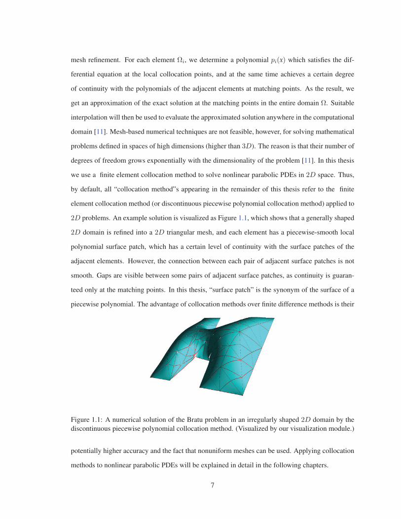
2D problems. An example solution is visualized as Figure 1.1, which shows that a generally shaped
2D domain is refined into a 2D triangular mesh, and each element has a piecewise-smooth local
polynomial surface patch, which has a certain level of continuity with the surface patches of the
adjacent elements. However, the connection between each pair of adjacent surface patches is not
smooth. Gaps are visible between some pairs of adjacent surface patches, as continuity is guaran-
teed only at the matching points. In this thesis, “surface patch” is the synonym of the surface of a
piecewise polynomial. The advantage of collocation methods over finite difference methods is their
Figure 1.1: A numerical solution of the Bratu problem in an irregularly shaped 2D domain by thediscontinuous piecewise polynomial collocation method. (Visualized by our visualization module.)
potentially higher accuracy and the fact that nonuniform meshes can be used. Applying collocation
methods to nonlinear parabolic PDEs will be explained in detail in the following chapters.
7
1.5 Organization of the thesis
This thesis is organized as follows. Chapter 1 gives an overview of the classification of PDEs
and the numerical methods, where the collocation method is also briefly introduced. Chapter 2 de-
scribes triangulation of irregularly shaped problem domains and generation of adaptive triangular
meshes over the domains. The Rivara algorithm is also introduced. In Chapter 3, we explain in
detail the principle of the collocation method. In Chapter 4, we extend the local system of the piece-
wise collocation method from a single element to the subdivision hierarchy. We also estimate the
complexity of the method. Chapter 5 describes the software architecture and data structure. Chapter
6 discusses five test PDEs and an application of the collocation method to the Bratu problem. From
the large number of the test results we find the configurations of collocation points and matching
points which bring high accuracy and best performance. Chapter 7 is dedicated to explaining the
principle and algorithms of our 3D visualization program. In Chapter 8, we give a summary and
conclusions of the research, and we point to several possible improvements.
8

Chapter 2
Mesh Generation
As shown in Figure 1.1 in Section 1.4, the collocation method for solving 2D PDEs relies on
discretizing the problem domain with 2D meshes. In this chapter we discuss 2D mesh generation.
The generation of 3D mesh, which is necessary for a 3D collocation method, is also mentioned
briefly at the end of this chapter.
2.1 Local adaptive mesh refinement
The 2D mesh for our collocation method is a triangular mesh, composed of triangular elements
only. In some other implementations of the collocation method, square-element meshes have been
used [17], [27], [28]. However, square (or more generally, quadrilateral) elements have two main
limitations. First, a quadrilateral-element mesh cannot easily support locally adaptive mesh re-
finement. Local refinement refers to recursively subdividing only the local regions where smaller
elements are needed to reach the required accuracy. The recursive subdivisions must be limited to
the local regions and not spread over the global domain. Based on locally refined meshes, collo-
cation methods can achieve high accuracy with fewer elements, thereby at less computational cost,
in comparison to using globally refined meshes. However, refinement in any square element must
spread to all elements that are geometrically adjacent in horizontal and / or vertical directions in the
span of the global domain. Therefore, square elements do not easily support local refinement. For
9

general quadrilateral-element meshes, local refinement usually cannot be achieved, either. Trian-
gular meshes support local refinement; two locally adaptive triangle meshes generated by Rivara’s
refinement algorithm ([42],[46]) are shown in Figure 2.1 and 2.3.
Figure 2.1: A locally refined triangularmesh adapted to a 2D Gaussian func-tion.
Figure 2.2: The profile of the 2D Gaus-sian function from [30]
Figure 2.3: A locally refined triangularmesh adapted to an ideal 2D low-passfilter Figure 2.4: The ideal 2D low-pass filter
Evaluation methods are needed by locally adaptive mesh refinement schemes to determine
whether a region needs to be further refined or not. The evaluation methods estimate local er-
rors. If an estimated local error is larger than a given threshold, then continue to locally refine the
related elements. “Mesh adaptation is based on a posteriori error estimator or error indicator that is
evaluated in function of the current numerical solution at each discrete place of the mesh” [44]. For
10

finite element methods, a Posteriori Error Estimation techniques have been developed [34][35][36].
For the collocation method there is no existing theoretically proved local error estimator. Thus
evaluation methods for collocation methods evaluate error indicators instead of directly estimating
errors. An error indicator can approximately reflect how big the local error could be. One practically
used error indicator is the absolute difference between the two (n− 1)th order outward directional
derivatives of the two n degree polynomials over each pair of neighboring elements at each of their
matching points. (The outward directional derivative will be explained in Section 3.2 by Figure 3.1
and equation (3.12)) If such error indicator is larger than a specified threshold, the elements need
to be further refined. In this thesis we have tried another error indicator, which computes the quasi-
curvature of the polynomial surface patch over each element. If the quasi-curvature of a polynomial
surface patch is larger than a certain threshold, the corresponding element will be further refined.
The quasi-curvature is calculated the way illustrated in Figure 2.5. Triangle ABC is an element.
Figure 2.5: Measuring how much a piecewise polynomial surface is bent. The picture on the rightside simplifies the view of 3D into 2D, where the curve represents the surface, and L represents theplane of triangle A′B′C ′.
A′B′C ′ is the surface patch over element ABC. α is the plane defined by the vertices A′, B′, and
C ′. To measure how much A′B′C ′ is bent, i.e., its quasi-curvature, we follow the steps below:
(1) Choose one or multiple sample points inside element ABC, such as the S in Figure 2.5.
(2) Emit a line from S, perpendicular to the plane of ABC and towards the surface patch A′B′C ′;as a result, the line intersects with the plane α at the point S′.
11
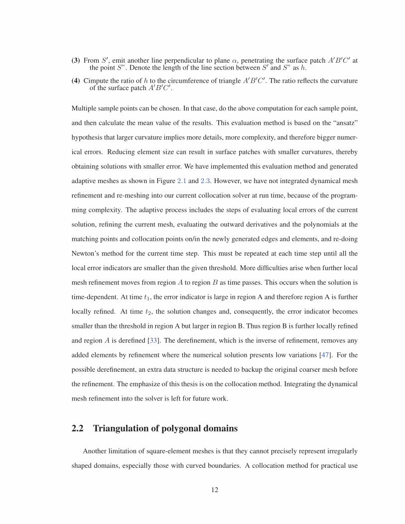
(3) From S′, emit another line perpendicular to plane α, penetrating the surface patch A′B′C ′ atthe point S”. Denote the length of the line section between S′ and S” as h.
(4) Cimpute the ratio of h to the circumference of triangle A′B′C ′. The ratio reflects the curvatureof the surface patch A′B′C ′.
Multiple sample points can be chosen. In that case, do the above computation for each sample point,
and then calculate the mean value of the results. This evaluation method is based on the “ansatz”
hypothesis that larger curvature implies more details, more complexity, and therefore bigger numer-
ical errors. Reducing element size can result in surface patches with smaller curvatures, thereby
obtaining solutions with smaller error. We have implemented this evaluation method and generated
adaptive meshes as shown in Figure 2.1 and 2.3. However, we have not integrated dynamical mesh
refinement and re-meshing into our current collocation solver at run time, because of the program-
ming complexity. The adaptive process includes the steps of evaluating local errors of the current
solution, refining the current mesh, evaluating the outward derivatives and the polynomials at the
matching points and collocation points on/in the newly generated edges and elements, and re-doing
Newton’s method for the current time step. This must be repeated at each time step until all the
local error indicators are smaller than the given threshold. More difficulties arise when further local
mesh refinement moves from region A to region B as time passes. This occurs when the solution is
time-dependent. At time t1, the error indicator is large in region A and therefore region A is further
locally refined. At time t2, the solution changes and, consequently, the error indicator becomes
smaller than the threshold in region A but larger in region B. Thus region B is further locally refined
and region A is derefined [33]. The derefinement, which is the inverse of refinement, removes any
added elements by refinement where the numerical solution presents low variations [47]. For the
possible derefinement, an extra data structure is needed to backup the original coarser mesh before
the refinement. The emphasize of this thesis is on the collocation method. Integrating the dynamical
mesh refinement into the solver is left for future work.
2.2 Triangulation of polygonal domains
Another limitation of square-element meshes is that they cannot precisely represent irregularly
shaped domains, especially those with curved boundaries. A collocation method for practical use
12

must be applicable to domains of general shape. For simplicity, in this thesis we consider only
polygonal domains with unique boundary. Triangular elements can cover such domains, as illus-
trated in Figure 2.3. Our solver can generate meshes for irregularly shaped polygonal domains by
triangulation and by refining the resulting triangles into final elements. Some examples are shown
in Figures 2.7 and 2.9. Triangulation should be optimized to result in well-shaped triangles; other-
wise, as the result of refinement, some elements will also have poor shapes. The shapes of elements
in a mesh have a pronounced effect on numerical methods [31][32]. The aspect Ratio, defined to be
the ratio of the maximum and the minimum widths of an element [31][32], is introduced to measure
how good (or poor) its shape is. “In general, elements of large aspect ratio are bad. Large aspect
ratios can lead to poorly conditioned matrices, worsening the speed and accuracy of linear solver”
[31]. Elements of poor aspect ratio however, can seriously degrade accuracy [32]. Two types of
shapes with large aspect ratios are given in Figure 2.6. Our current triangulation algorithm does
not optimize shapes. It simply recursively cuts off the first convex corner it detects in the remain-
ing polygon without evaluating the shape of the new triangle. As a result, there may exist large
aspect ratio elements in the result meshes of the triangulation. Even so, our tests indicate that, with
local coordinates, our collocation method still converges and obtains accurate solutions with such
meshes. Only in some extreme cases, we observe less local accuracy and / or poor convergence
(i.e., more Newton iterations are needed for the convergence, or we have nonconvergence) caused
by large aspect ratio elements. Tests also show that the collocation method becomes more sensitive
to large aspect ratio shapes when not using local coordinates. The optimization of triangulation is
not a focus of this these. It is expected that users of our collocation method solver have made a
good triangulation and then, based on the result of the triangulation, our solver performs further
refinement if necessary. In Section 2.5, we will talk about our collocation method using existing
meshes.
2.3 The Rivara algorithm
Given a well shaped triangulation, the next step is to construct a locally refined triangulation,
such that the smallest (or the largest) angle is bounded [45]. The refinement process is continued
13

Figure 2.6: Shapes with large aspect ratios: (a) angle too large; (b) angle too small.
Figure 2.7: (a) Generating a triangularmesh by triangulation.
Figure 2.8: (b) Refinement of the trian-gular mesh.
Figure 2.9: (a) Generating a triangularmesh by triangulation.
Figure 2.10: (b) Refinement of the tri-angular mesh.
14

recursively until the evaluation criterion is satisfied. Nesting is an expected feature of candidate
refinement algorithms, “i.e., the triangles in the refined mesh are nested within the previous mesh
level. Moreover, nesting means that a unique discrete place generates others without changing the
edges and coordinates of its neighbors in a refinement process. This process may provide low
computational cost because few nodes of the data structure should be traversed and updated in order
to correctly represent the new mesh.”[44] There are various triangulation refinement algorithms,
as described in [44], among which we choose the Rivara algorithm. The Rivara algorithm can be
described as follows:
(1) Scan all triangles one-by-one. When encountering an “un-refined” triangle Δ1, evaluate whether
it needs to be refined using the error estimate. If yes, insert a new edge, l1, into it, which links
the midpoint of its longest edge, L1, to the opposite vertex. Δ1 is thereby bisected into two
new triangles, Δ11 and Δ12. Δ11 and Δ12 are called sibling nodes, which is a critically im-
portant concept in the nested dissection explained in Section 4.2. A pair of geometrically
adjacent nodes are neighboring, but not necessarily sibling. Only a pair of neighboring nodes
which are generated by bisecting the parent node are sibling nodes.
(2) If the bisected edge, L1, is shared by Δ1 and its neighboring triangle Δ2, L1 is called pending
edge until Δ2 is accordingly subdivided in either one of the following ways:
(2.1) If L1 is also the longest edge of Δ2, insert a new edge, l2, into Δ2, connecting the
midpoint of L1 to the opposite vertex in Δ2, thereby generating Δ21 and Δ22. Then go
to step (1) to detect next un-refined triangle.
(2.2) Otherwise, the longest edge of Δ2 is L2. Then bisect L2, connect the midpoint of L2
to the opposite vertex, thereby generating Δ21 and Δ22. Then, link the midpoint of L2
to the midpoint of L1, thereby generating Δ211 and Δ212 (or Δ221 and Δ222, depending
on whether L1 is in Δ21 or Δ22). Finally, check whether L2 is a pending edge. If yes,
there exists a neighbor Δ3, so, go to step (2) to work on Δ3; if no, go to step (1) to work
on next un-refined triangle.
Mark each new triangles as “already refined” as soon as it is generated in order to prevent
them from being refined again in the current round of refinement.
15

(3) When all triangles have been processed then the current round of refinement is completed. Reset
all the triangles to “un-refined”, and then start the next round of refinement. Repeat this loop
until no more refinement is needed. The jth round corresponds to the jth level of refinement.
Rosenberg and Stenger have proved that the interior angles do not go to zero as the level of
refinement tends to infinite (i.e., j → ∞). Specifically, if α is the smallest interior angle of the
originally given triangle, and θ is any interior angle of the new triangles generated at the jth level of
refinement, then θ � α/2 [44]. The Rivara refinement maintains the feature that any interior angle
of the resulting triangles is bounded away from 0 or π and the resulting triangles satisfy a shape
regularity property [44]. In addition, the Rivara algorithm has been proven to terminate in a regular
mesh in a finite number of steps [20]. The algorithm has also the advantage that since it is a local
refinement operation it can be parallelized to deal with the refinement of very large meshes [44].
The steps of the refinement processes are illustrated in Figure 2.11 and 2.12.
Figure 2.11: A domain triangulated andrefined at the first level.
Figure 2.12: The domain after 2 levelsof refinement: level 1 and 2.
2.4 3D mesh refinement
The significance of generalizing the 2D adaptive mesh refinement algorithms discussed in the
preceding sections, such as the Rivara algorithm, to 3D mesh generation is obvious. “Adaptivity
of the mesh is particularly important in three-dimensional problems because the problem size and
computational cost grow very rapidly as the mesh size is reduced” [49]. Much research has been
done on this problem.
16

“Rivara and Levin suggested an extension of longest-edge Rivara refinement to three dimen-
sions. . . . Rivara and Levin provide experimental evidence suggesting that repeated rounds of
longest-edge refinement cannot reduce the minimum solid angle below a fixed threshold, but this
gurantee has not been mathematically proved.” [31, 115]
In [40], A. Selman, A. Merrouche, and C. Knopf-Lenoir have presented and implemented adap-
tive 3D refinement procedures for tetrahedral meshes using the bisection and Rivara algorithms
based on an explicit mesh density function coupled with an automatic 3D mesh generator which
subdivides 3D problem domains into assemblies of tetrahedral elements [40]. Furthermore, they
have also given benchmark examples to measure the performance of their refinement methods in
terms of the following criteria specified in [40]:
- produce meshes of a desired density,
- generate conforming elements of good quality, and
- avoid the generation of an excessive number of elements (nodes).
Their conclusion is that the Rivara 3D algorithm produces meshes of optimal quality.
In [49], Angel Plaza, Miguel A. Padron, and Graham F. Carey have presented and discussed
several practical 3D local refinement/derefinement algorithms for tetrahedron meshes. They state
the following: “There are still several open questions related to a mathematical proof of the non-
degeneracy of the meshes obtained, and the existence of a bounded number of similarity classes
(that, perhaps, depend on the geometry of the initial 3D triangulation). Although theses properties
have been proved in two dimensions, the generalization to three dimensions is not yet solved” [49].
And in [42], M.-C. Rivara points out that “even when the algorithms have been successfully used
in practice in 3D, a theory on (longest edge) bisection in 3-dimensions such as that presented for
2-dimensions has not been yet developed”.
In conclusion, many 3D mesh refinement/derefinement algorithms have been presented, imple-
mented, and practically applied to solving numerical problems. However, in theory it is still an open
problem to mathematically prove whether (longest edge) bisection algorithms (such as the Rivara
algorithm) can terminate in a finite number of steps with a regular mesh that has its smallest interior
angle bounded. Meshes and problems in 3D are outside the scope of this thesis.
17

2.5 Other mesh generation methods
In Section 2.2, we have introduced a simple method of triangulation, which in some cases may
result in regions with large aspect ratios and thereby lead to less accuracy, poorly conditioned matri-
ces, or lower rate of convergence. Fortunately, there exist other mature triangulation methods, such
as the Delaunay triangulation and refinement. From a mesh generated by the Delaunay algorithm,
we must construct a hierarchy of recursive subdivisions, which is required by our nested dissection
discussed in Section 4.2. The hierarchy of subdivisions is expressed as a binary tree, called subdi-
vision tree, each internal node of which represents subdividing a region Ω into two subregions, Ω1
and Ω2, where Ω1 ∪ Ω2 = Ω and Ω1 ∩ Ω2 = 0. The border-line between Ω1 and Ω2 is an arbitrary
polyline and not necessarily a straight line as required in the subdivision by the Rivara algorithm. In
the context of parallel computing, the computational tasks in the two sub-trees under the subregions
Ω1 and Ω2 are assigned respectively to two threads running in parallel. For balancing the workload
of the two threads, the subregions Ω1 and Ω2 should be composed of a nearly equal number of
elements. For minimizing interference between the two concurrent computational tasks, Ω should
be appropriately bisected to minimize the length of the border-line between the subregions Ω1 and
Ω2. There may be various ways to generate subdivision trees from existing meshes. As long as a
subdivision tree is generated, we can then proceed the nested dissection on the subdivision tree.
Additionally, as mentioned in Section 2.4, the extension of the longest-edge Rivara refinement to
3D is not mathematically proved. Therefore, if we want to expand the application of our collocation
method and nested dissection to 3D space, we will have to choose some other well proved 3D mesh
generation algorithms, such as the Delaunay triangulation and refinement.
18
Chapter 3
A Collocation Method for Nonlinear
Parabolic PDE BVP
In this chapter we will explain the principle of the piecewise collocation method and how it is
applied to solving nonlinear parabolic PDEs. Throughout this thesis, we will follow the notation
defined below:
– X = (x, y)T ∈ R2 is the spatial variable.
– zMi represents a matching point, and zCj represents a collocation point.
– u represents the exact solution of PDEs.
– �u = (u1, u2, . . . , uk)T where ui is the value of u evaluated at a matching point zMi, and k is
the number of these matching points.
– �v = (v1, v2, . . . , uk)T where vi is the directional derivative of u evaluated at a matching point
zMi in the outward direction, and k is the number of these matching points.
– p represents the polynomial values used for approximating the solution of PDEs.
These items will be explained in the following sections.
3.1 Nonlinear parabolic PDE problems
The piecewise polynomial collocation method is efficient for solving boundary value problems
of ODEs and PDEs. In this thesis we apply the collocation method to solving 2D parabolic PDEs
19
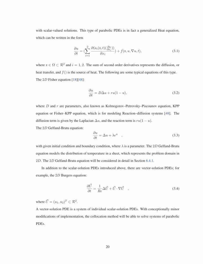
with scalar-valued solutions. This type of parabolic PDEs is in fact a generalized Heat equation,
which can be written in the form
∂u
∂t= (
2∑i=1
∂(ai(X, t)( ∂u∂xi
))
∂xi) + f(X, u,∇u, t), (3.1)
where X ∈ Ω ⊂ R2 and i = 1, 2. The sum of second order derivatives represents the diffusion, or
heat transfer, and f() is the source of heat. The following are some typical equations of this type.
The 2D Fisher equation [18][48]:
∂u
∂t= DΔu+ ru(1− u), (3.2)
where D and r are parameters, also known as Kolmogorov–Petrovsky–Piscounov equation, KPP
equation or Fisher–KPP equation, which is for modeling Reaction–diffusion systems [48]. The
diffusion term is given by the Laplacian Δu, and the reaction term is ru(1− u).
The 2D Gelfand-Bratu equation:∂u
∂t= Δu+ λeu , (3.3)
with given initial condition and boundary condition, where λ is a parameter. The 2D Gelfand-Bratu
equation models the distribution of temperature in a sheet, which represents the problem domain in
2D. The 2D Gelfand-Bratu equation will be considered in detail in Section 6.4.1.
In addition to the scalar-solution PDEs introduced above, there are vector-solution PDEs; for
example, the 2D Burgers equation:
∂�U
∂t=
1
ReΔ�U + �U · ∇�U , (3.4)
where �U = (u1, u2)T ⊂ R2.
A vector-solution PDE is a system of individual scalar-solution PDEs. With conceptionally minor
modifications of implementation, the collocation method will be able to solve systems of parabolic
PDEs.
20

3.2 Collocation with discontinuous piecewise polynomials
The collocation method presented in this thesis for solving nonlinear parabolic PDEs is derived
from the idea used for elliptic PDEs by E. J. Doedel in [27][28] and for nonlinear elliptic PDE BVP
by Sharifi in [17]. We give a quick review of collocation methods for ODEs and PDEs. A dis-
continuous piecewise polynomial collocation method has been used by Doedel for developing the
AUTO package, which is one of the most widely used continuation and bifurcation analysis soft-
ware packages for ODE problems [17]. Doedel has generalized this method for solving linear and
nonlinear elliptic PDEs [27][28]. Sharifi generalized the method for solving linear and nonlinear el-
liptic PDE systems using an alternative nested dissection solution procedure [17]. In his Ph.D thesis,
Sharifi introduced the use of this method for solving linear and nonlinear PDEs. He has developed
an AUTO-like continuation prototype for solving linear and nonlinear elliptic PDEs in 2D space
[17].The method and the prototype implementation of Doedel and Sharifi are based on a square
mesh. As explained in Chapter 2, a square mesh has its limitations. Zheng Qiang implemented a
linear parabolic PDE solver based on the collocation method with adaptive triangular meshes [20].
Also based on the work of Doedel and Sharifi, are the results of He, Sun, Wu, and Zhang, who
have derived error estimates for some specific collocation schemes for square or triangular meshes.
In this thesis we further extend the use of the collocation method to nonlinear parabolic PDEs in
irregular polygonal domains, using triangular meshes.
Our goal is to solve parabolic PDEs of the general form
∂u
∂t= Δu+ f(X, u,∇u, t), X = (x, y) ∈ Ω ⊂ R2, u, f ⊂ R, (3.5)
where Δ is the Laplacian operator, ∇ is the operator of gradient; in R2, namely, ( ∂∂x ,
∂∂y )
T , and
f(X, u,∇u, t) is linear or nonlinear function of u and ∇u. We specify a function D(X) as boundary
condition
u(X) = D(X), X ∈ δΩ. (3.6)
21

For the temporal dimension, we use the Backward Euler method to discretize the partial differential
derivatives with respect to time.
uk − uk−1δt
= Δuk + f(X, uk,∇uk, tk), k = 1, 2, 3, . . . (3.7)
where δt represents time interval and k is the index of the time steps. Multistep finite difference
methods can also be used to improve the numerical accuracy with respect to δt; however, they bring
additional complexity to the implementation. For the purpose of testing the collocation method, the
Euler method is sufficient.
Introducing the nonlinear operator N , we can rewrite equation (3.7) as
Nuk = Δuk + f(X, uk,∇uk, tk)− ukδt
+uk−1δt
= Δuk + h(X, uk,∇uk, tk)
= 0, k = 1, 2, 3, . . . , n ,
(3.8)
where
h(X, uk,∇uk, tk) = f(X, uk,∇uk, tk)− ukδt
+uk−1δt
,
uk is the unknown to solve for at tk, and uk−1
δt is a constant.
For the spatial dimensions, we generate a mesh over the problem domain as discussed in Chapter
2. As shown in Figure 3.1 and 3.2, the zci are local collocation points (where the ’c’ stands for
”collocation”), the zMj are local matching points (, where the ’M ’ refers to ”matching point”), and
the ηj are unit outwards vectors at the zMj . For each element we need to construct a polynomial of
the following form to approximate the exact solution u(X):
u(X) ≈ p(X) =n+m∑i=1
ciφi(X), p() ∈ Pn+m, (3.9)
where n and m are the number of local matching points and collocation points, respectively. The
ci are the unknown constant coefficients to be solved for. Such ci are not related to the ’ci’ in
’zci’which stand for “Collocation point”. The set {φ1, . . . , φm+n} is a specific basis, and Pn+m =
22

Figure 3.1: A triangular mesh for the2D collocation method.
Figure 3.2: Collocation and matchingpoints of an element.
Span{φ1, . . . , φm+n} is the polynomial space of dimension n+m. The following two conditions
must be satisfied by p. First, p must satisfy the collocation equation; that is, p satisfy the PDE at
each of the collocation points.
Np(zci) = 0, i = 1, 2, 3, . . . ,m, (3.10)
where N is the nonlinear operator defined in (3.8), and the zci are the local collocation points.
Secondly, p must have a certain degree of continuity with the polynomials of its adjacent elements;
that is, each pair of adjacent polynomials must have the same value of ui at each of the matching
points zMi they share:
p(zMi) = u(zMi) = ui , (3.11)
and they must also have the same derivative in the direction of the outward normal at the matching
point:
ηi · (∇p(zMi))T = ηi · (∇c1φ1(zMi)
T + · · ·+∇cn+mφn+m(zMi)T ) = vi (3.12)
Since the two outward normal vectors of each pair of sibling elements point in opposite direction, the
derivatives of the two polynomials projected onto these two outward normal vectors have different
23

signs. Let
�u =
(u1:un
)δ�u =
(δu1:
δun
)�v =
(v1:vn
)δ�v =
(δv1:
δvn
)�c =
(c1:
cn+m
)δ�c =
(δc1:
δcn+m
),
adhere �u and δ�u are written in explicit vector form to distinguish them from the u in (3.5).
Let
Φ =
⎛⎜⎜⎜⎜⎝
φ1(zM1) · · · φ1(zMn)
: :
φn+m(zM1) · · · φn+m(zMn)
⎞⎟⎟⎟⎟⎠ , (3.13)
and
RΦ =
⎛⎜⎜⎜⎜⎝
η1 ·∇φ1(zM1)T . . . ηn ·∇φ1(zMn)
T
: . . . :
η1 ·∇φn+m(zM1)T . . . ηn ·∇φn+m(zMn)
T
⎞⎟⎟⎟⎟⎠ . (3.14)
Then the continuity equations can be written as
(a) �u− ΦT�c = 0, (b) �v −RTΦ�c = 0. (3.15)
In summary, the principle of 2D collocation method is to solve the unknown �c of the collocation
equation (3.10) and the continuity equation (3.15) for an element. We use Newthon’s method to
solve these equations.
3.3 Newton’s method
To solve for the unknown �c ∈ Rn+m of (3.10) and (3.15) using Newton’s method, we need
to construct the corresponding linearized formulation. First, set up the residual formulation. The
residual formulation of (3.10) is
�rN =
(Np(zC1)
:Np(zCm)
). (3.16)
24

The linearization (i.e., Jacobian) of �rN about �c is
JrNc =
∂�rN∂�c
=
⎛⎜⎜⎜⎜⎝
∂Np(zC1)∂c1
. . . ∂Np(zC1)∂cn+m
: . . . :
∂Np(zCm)∂c1
. . . ∂Np(zCm)∂cn+m
⎞⎟⎟⎟⎟⎠ . (3.17)
We use LΦ to denote (JrNc )T and Li(zj) to denote ∂Np(zj)
∂ci. By transposing, we make the elements
of LΦ arranged as those of matrix Φ in (3.13) and the matrix RΦ in (3.14).
LΦ =
⎛⎜⎜⎜⎜⎝
L1(zC1) · · · L1(zCm)
: :
Ln+m(zC1) · · · Ln+m(zCm)
⎞⎟⎟⎟⎟⎠ =
⎛⎜⎜⎜⎜⎝
∂Np(zC1)∂c1
· · · ∂Np(zCm)∂c1
: :
∂Np(zC1)∂cn+m
· · · ∂Np(zCm)∂cn+m
⎞⎟⎟⎟⎟⎠ . (3.18)
From (3.8), we have
Np = Δp+ h(X, p,∇p, t),
thus, the general form of the elements in matrix LΦ in (3.18) is
∂Np
∂ci=
∂(Δp+ h(X, p,∇p, t))
∂ci
=∂(c1Δφ1 + · · ·+ ciΔφi + · · ·+ cn+mΔφn+m)
∂ci+
∂h(X, p,∇p, t)
∂ci
= Δφi +∂h(X, p,∇p, t)
∂ci
= Δφi +∂h
∂p
∂p
∂ci+
∂h
∂∇p· ∂∇p
∂ci
= Δφi +∂h
∂pφi +
∂h
∂∇p· ∇φi
Recall that, in order to simplify the form of nonlinear operator N in (3.8), we have introduced h()
defined as
h(X, uk,∇uk, tk) = f(X, uk,∇uk, tk)− ukδt
+uk−1δt
,
25
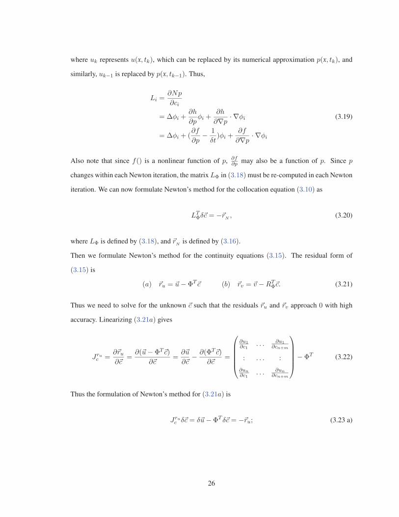
where uk represents u(X, tk), which can be replaced by its numerical approximation p(X, tk), and
similarly, uk−1 is replaced by p(X, tk−1). Thus,
Li =∂Np
∂ci
= Δφi +∂h
∂pφi +
∂h
∂∇p· ∇φi
= Δφi + (∂f
∂p− 1
δt)φi +
∂f
∂∇p· ∇φi
(3.19)
Also note that since f() is a nonlinear function of p, ∂f∂p may also be a function of p. Since p
changes within each Newton iteration, the matrix LΦ in (3.18) must be re-computed in each Newton
iteration. We can now formulate Newton’s method for the collocation equation (3.10) as
LTΦδ�c = −�rN , (3.20)
where LΦ is defined by (3.18), and �rN is defined by (3.16).
Then we formulate Newton’s method for the continuity equations (3.15). The residual form of
(3.15) is
(a) �ru = �u− ΦT�c (b) �rv = �v −RTΦ�c. (3.21)
Thus we need to solve for the unknown �c such that the residuals �ru and �rv approach 0 with high
accuracy. Linearizing (3.21a) gives
Jruc =
∂�ru∂�c
=∂(�u− ΦT�c)
∂�c=
∂�u
∂�c− ∂(ΦT�c)
∂�c=
⎛⎜⎜⎜⎜⎝
∂u1∂c1
. . . ∂u1∂cn+m
: . . . :
∂un∂c1
. . . ∂un∂cn+m
⎞⎟⎟⎟⎟⎠− ΦT (3.22)
Thus the formulation of Newton’s method for (3.21a) is
Jruc δ�c = δ�u− ΦT δ�c = −�ru; (3.23 a)
26

Similarly, the formulation of Newton’s method for (3.21b) is
Jrvc δ�c = δ�v −RT
Φδ�c = −�rv. (3.23 b)
We now have a linear system composed of (3.20), (3.23a), and (3.23b), the unknown of which is
δ�c. Rewrite the equations (3.23a) and (3.20) in the form
(ΦT
LTΦ
)δ�c =
(δ�u+ �ru−�rN
). (3.24)
Using (3.24) to substitute the δ�c in (3.23b), we have
δ�v = RTΦ
(ΦT
LTΦ
)−1 (δ�u+ �ru−�rN
)− �rv.
Let A be a n× n matrix and let B be the n×m matrix so that
(A|B) = RTΦ
(ΦT
LTΦ
)−1. (3.25)
Then we haveδ�v = (A|B)
(δ�u+ �ru−�rN
)− �rv,
which is equivalent toδ�v = Aδ�u−B �rN − �rv +A�ru . (3.26)
Let�g = −B �rN − �rv +A�ru. (3.27)
A and B can be solved from (3.25). However (3.25) is a conceptual formulation. In fact, we do not
compute the inverse matrix. Instead, we solve A and B by LU-decomposition of the matrix:
(Φ|LΦ)
(AT
BT
)= RΦ (3.28)
It is important to note that (Φ|LΦ) may be non-invertible (i.e., singular) for certain choices of the
basis functions, the number and location of matching points, or the number of collocation points.
We now present a brief discussion of the singularity of (Φ|LΦ) based on our observations.
27

If (Φ|LΦ) is singular then there exists a nonzero vector �a = (a1, . . . , an+m)T ∈ Rn+m such that
(ΦT
LTΦ
)�a = 0 , (3.29)
which means
S1(X) = a1φ1(X) + · · ·+ an+mφn+m(X) = 0 , (3.30)
at all the matching points {zM1, zM2, . . . , zMn} of an element, and simultaneously,
S2(X) = a1L1(X) + · · ·+ an+mLn+m(X) = 0 , (3.31)
where Li is defined in (3.18) and (3.19), at all collocation points {zC1, zC2, . . . , zCm} of the same
element. The geometrical significance of Equation (3.30) and (3.31) is that the surface S1(X) passes
through all the matching points, and at the same time, the surface S2(X) passes through all the
collocation points. Furthermore, because the surfaces S1(X) and S2(X) are smooth enough, they
must intersect with the plane of (x, y) at least near the matching points and collocation points.
Thus, we have the curves shown in Figure 3.3 and 3.4. Our collocation method solver can plot such
Figure 3.3: 4x3 matching points with 3collocation points.
Figure 3.4: 6x3 matching points with 10collocation points.
28

curves when (Φ|LΦ) is singular. Rewrite Equation (3.29) in the form
⎧⎪⎪⎪⎪⎪⎪⎪⎪⎪⎪⎪⎪⎪⎪⎪⎪⎪⎨⎪⎪⎪⎪⎪⎪⎪⎪⎪⎪⎪⎪⎪⎪⎪⎪⎪⎩
a1Φ1(zM1) + a2Φ2(zM1) + · · · + an+mΦn+m(zM1) = 0 (1)
a1Φ1(zM2) + a2Φ2(zM2) + · · · + an+mΦn+m(zM2) = 0 (2)
......
. . ....
......
a1Φ1(zMn) + a2Φ2(zMn) + · · · + an+mΦn+m(zMn) = 0 (n)
a1L1(zC1) + a2L2(zC1) + · · · + an+mLn+m(zC1) = 0 (n+ 1)
......
. . ....
......
a1L1(zCm) + a2L2(zCm) + · · · + an+mLn+m(zCm) = 0 (n+m)
, (3.32)
where the a1, . . . , an+m are the unknowns and Li is defined in (3.19). It is easy to see that system
(3.32) is composed of n + m equations for the n + m unknowns. Since the R.H.S of (3.32) is
zero, and if there are really n +m equations for n +m unknowns, there would not be a nontrivial
solution. However, (Φ|LΦ) being singular implies that there must be nontrivial solution for the
n + m unknown ai. Thus, the only possible conclusion is that some of the equations are linearly
dependent. This means that, for every Φi or Li, its values at some matching points or collocation
points are linearly dependent. For instance, assume equations (1), (2), and (n) in (3.32) are linearly
dependent, thus
b1(1) + b2(2) + b3(n) = 0 ,
the related matching points are zM1, zM2, and zMn. Then there must be the same linear dependence
for every Φi, as shown below:
b1Φ1(zM1) + b2Φ1(zM2) + b3Φ1(zMn) = 0 ,
b1Φ2(zM1) + b2Φ2(zM2) + b3Φ2(zMn) = 0 ,
. . . . . .
b1Φn(zM1) + b2Φn(zM2) + b3Φn(zMn) = 0 ,
b1Φn+1(zM1) + b2Φn+1(zM2) + b3Φn+1(zMn) = 0 ,
. . . . . .
b1Φn+m(zM1) + b2Φn+m(zM2) + b3Φn+m(zMn) = 0 .
29

Our tests and observations show that this type of linear dependence does exist at matching points
(not collocation points) if
– there are at least 3 matching points per edge of an element, and
– the matching points on the same edge are regularly (for example, evenly or symmetrically)distributed, and
– n + m is not large enough with respect to n, where n and m are the numbers of matchingpoints and collocation points per element, respectively; therefore, this linear dependence caneasily take place to every Φi, as illustrated in the above example.
The existence of such linear dependence is a necessary condition for the singularity. In the case
shown in Figure 3.3, the matrix (Φ|LΦ) has been shown to be singular by our tests. Further ex-
periments indicate that we can make the (Φ|LΦ) non-singular by moving any one matching point
either away from the edge, to reduce the number of collinear matching points, or along the edge to
make the distribution of matching points less regular. However, neither of the moves is acceptable
because matching points must be on the edges and regularly distributed. A correct way to avoid the
singularity is to add more collocation points and thereby increase the ratio of n+m to n.
This necessary condition can be equivalently expressed like the following: after Gaussian Elim-
ination on (Φ|LΦ), the resulting (n+m)× (n+m) matrix M is of the form (3.33).
M =
⎛⎜⎜⎜⎜⎜⎜⎜⎜⎜⎜⎜⎜⎜⎜⎜⎜⎜⎝
× × × . . . × × × . . . ×0 × × . . . × × × . . . ×0 0 × . . . × × × . . . ×0 0 0 . . . × × × . . . ×: : : . . . : : × . . . ×0 0 0 . . . × × × . . . ×0 0 0 . . . 0 0 × . . . ×0 0 0 . . . 0 0 0 . . . ×: : : . . . : : : . . . :
0 0 0 . . . 0 0 0 . . . 0
⎞⎟⎟⎟⎟⎟⎟⎟⎟⎟⎟⎟⎟⎟⎟⎟⎟⎟⎠
(3.33)
The square block in the frame is a n × n sub-matrix, which corresponds to the n matching points.
The sub-matrix has an all-zero row, which means that the sub-matrix is singular and there exists a
curve
S0(X) = a1φ1(X) + · · ·+ anφn(X) = 0 ,
which passes through all the n matching points. Thus, the existence of such a curve is the necessary
30

condition of (Φ|LΦ) being singular. In the case of 1 matching point per edge, there are totally 3
matching points for an element. Because we use localized power polynomials as basis functions,
i.e., {φ1, φ2, φ3, φ4, φ5, φ6, . . . } = {1, (x−x0), (y−y0), (x−x0)(y−y0), (x−x0)2, (y−y0)
2, . . . }.
The reason for which we use local coordinates (x − x0) and (y − y0) will be explained in Section
3.4. The corresponding S0(X) is
S0(X) = a1φ1(X) + a2φ2(X) + a3φ3(X)
= b1 + b2x+ b3y
= 0, X = (x, y) ,
which is a straight line. It is impossible for a straight line to pass the 3 non-collinear matching points.
Thus, the necessary condition does not hold and, therefore, the (Φ|LΦ) of this case is nonsingular.
In the case of 2 matching points per edge, there are totally 2× 3 = 6 matching points per element,
and the curve
S0 = a1φ1 + a2φ2 + a3φ3 + a4φ4 + a5φ5 + a6φ6
= b1 + b2x+ b3y + b4x2 + b5xy + b6y
2
= 0 ,
is a conic section. According to the Bezout’s theorem, two conic sections generally intersect in
four points. This implies that 5 points, among which any 3 points are noncollinear, uniquely define
a conic section. Thus, there exists not any single conic passing through the 6 matching points in
this case. Thus, the necessary condition does not hold and, therefore, the (Φ|LΦ) of this case is
nonsingular.
Collocation points influence the singularity by the number rather than their locations. Our tests
show that, if (Φ|LΦ) is singular, then relocating the collocation points does not change the sin-
gularity. Figure 3.5 shows the same case as in Figure 3.4, with the collocation points rearranged.
However, the (Φ|LΦ) is still singular because the singularity is not caused by the location of the
collocation points. The function Li(X), defined in (3.18) and (3.19), depends not only on the basis
functions Φi, but also on the PDE. Thus, it is more difficult to analysis the linear dependence related
to the Li(X) at the collocation points. We only use the number of collocation points, m, to control
31

Figure 3.5: 6x3 matching points with 10 relocated collocation points.
the number of basis functions, n +m, as mentioned in the preceding paragraph. If n +m is large
enough with respect to a specific n, the singularity can be avoided. This has been confirmed by our
experiments.
3.4 The choice of basis polynomials
Because a numerical solution is a linear combination of basis polynomials, the accuracy of
the numerical solution depends heavily on the choice of basis polynomials. In this thesis we use
localized power basis polynomials, {1, (x−x0), (y−y0), (x−x0)(y−y0), (x−x0)2, (y−y0)
2, . . . },
because it is easy to compute their first and second order derivatives. The coordinate must be
localized and even normalized; otherwise, matrix (Φ|LΦ) may be ill-conditioned if some elements
are very small or have high aspect ratio (defined in Section 2.2), or the collocation and matching
points are not well located. We localize and normalize the coordinate by replacing x and y of the
basis functions with (x− x0)/L and (y − y0)/L, respectively, where (x0, y0) may be the center of
gravity or any vertex of the local element, and L is longest edge of the element.
Lagrange basis functions can also be used. An important feature of Lagrange basis functions
is that each of them is equal to 1 at a certain collocation point or matching point and equal to
0 at any other collocation point, matching point, and anywhere else in the domain. This feature
makes solving Equation (3.28) to obtain the matrices A and B much more efficient because the
matrix Φ = (I|0)T , where I represents the identity matrix. This is explained in [28] and [27]. A
32

Lagrange basis is easy to use with square meshes. For using a Lagrange basis with triangular meshes
in irregular domains, each arbitrary triangle must first be transformed to the Standard triangle by
affine transformation.
Bernstein basis functions can also be used for the collocation method. However, any Bernstein
polynomial can be written in terms of the power basis [37]. Thus, in substance, a Bernstein basis is
equivalent to the power basis.
3.5 The collocation method with initial and boundary conditions
In this section we will show how the equations and matrices presented in Section 3.2 and 3.3
are involved in the Newton iteration and the time integration to solve PDEs. To focus on the most
essential principles of our collocation method, in this section we will use a single-element triangle
mesh; that is, the problem domain is triangular and not refined. This is the global collocation
method mentioned in Section 1.4, which has more educational sense than practical use. It is a good
preparation for discussing the case of multi-element mesh, i.e., piecewise polynomial collocation
method, which will be explained in Chapter 4. The steps of the single-element mesh case are listed
below:
• Apply the initial condition to �u, �v, and �c;
• Compute Φ (3.13) and RΦ (3.14) only once, i.e.,do not re-compute them for all time steps;
• Loop of time integration; at each time step, do the following tasks:
◦ Loop of Newton iteration for solving equation (3.24), until sufficiently converged.In each loop of the iteration:∗ Compute LΦ (3.19); —– (1)∗ Solve (3.28) to get matrix A and B; —– (2)∗ Compute �rN (3.16), �ru, and �rv (3.21);∗ Construct system (3.26);∗ Compute the δ�u and δ�v on the boundary from B.C and (3.26); –(3)∗ Solve equation (3.24) (with the current LΦ, δ�u, �ru, and �rN ) to get the current δ�c;∗ �c+ = δ�c, �u+ = δ�u, �v+ = δ�v;
◦ Save the current �u, �v, and �c for the use as initial values and uk−1 when computing �rN(3.16), (3.8) at next time step;
• End.
Further discussion on the above steps marked with (1), (2), and (3):
For the sake of performance, and also for stability in some cases, (1) can be computed only in the
33
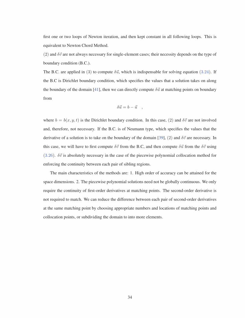
first one or two loops of Newton iteration, and then kept constant in all following loops. This is
equivalent to Newton Chord Method.
(2) and δ�v are not always necessary for single-element cases; their necessity depends on the type of
boundary condition (B.C.).
The B.C. are applied in (3) to compute δ�u, which is indispensable for solving equation (3.24). If
the B.C is Dirichlet boundary condition, which specifies the values that a solution takes on along
the boundary of the domain [41], then we can directly compute δ�u at matching points on boundary
from
δ�u = b− �u ,
where b = b(x, y, t) is the Dirichlet boundary condition. In this case, (2) and δ�v are not involved
and, therefore, not necessary. If the B.C. is of Neumann type, which specifies the values that the
derivative of a solution is to take on the boundary of the domain [39], (2) and δ�v are necessary. In
this case, we will have to first compute δ�v from the B.C, and then compute δ�u from the δ�v using
(3.26). δ�v is absolutely necessary in the case of the piecewise polynomial collocation method for
enforcing the continuity between each pair of sibling regions.
The main characteristics of the methods are: 1. High order of accuracy can be attained for the
space dimensions. 2. The piecewise polynomial solutions need not be globally continuous. We only
require the continuity of first-order derivatives at matching points. The second-order derivative is
not required to match. We can reduce the difference between each pair of second-order derivatives
at the same matching point by choosing appropriate numbers and locations of matching points and
collocation points, or subdividing the domain to into more elements.
34

Chapter 4
Numerical Linear Algebra
In Chapter 3 we have explained the essential principle of the collocation method. Based on
this principle we have constructed the local linear system (3.26) of an element. In this chapter we
discuss how to assemble all the local linear systems together to construct the global system and then
apply boundary conditions to numerically solve a PDE in the entire problem domain. The nested
dissection is introduced for solving the global system in parallel. This is a natural advantage of the
collocation method. Chapters 3 and 4 together explain the entire principle of piecewise polynomial
collocation method.
4.1 The global linear system
In Section 3.2, we mentioned that piecewise polynomial collocation method needs a mesh which
decomposes the problem domain into elements. The local linear system (3.26) of each element can
be re-written in the formDδ�v = Aδ�u+ �g, (4.1)
where D is initially an identity matrix for each element, and
�g = −B �rN − �rv +A�ru. (4.2)
Then we construct the global linear system from the local linear systems (4.1) of all elements. First,
we use an example to show how to do it. The problem domain of the example is illustrated in
35

Figure 4.1, which is discretized into 4 elements. Suppose there are k matching points per side of
Figure 4.1: The global domain Ω is composed of elements Ω1, Ω2, Ω3, and Ω4. i represents agroup of k matching points on one side of an element.
each element. We denote by δ�uij the δ�u of element Ωi at the k matching points on its edge shared
with a neighboring element Ωj . The order of ”ij” is not invertible because δ�uij and δ�uji refer to
different quantities, which are evaluated respectively by the two different polynomials of Ωi and
Ωj , although at the same matching point(s). The former is the local polynomial over Ωi, whereas
the latter is the local polynomial over Ωj . Similarly, δ�vij and δ�vji are also denoted this way. If the
edge is a part of the boundary of the entire domain, there is not any other element on the other side
of the edge. Thus, the δ�u and δ�v on such kind of edges are denoted as δ�ui and δ�vi, respectively.
For example, at 2 , δ�u12 and δ�v12 are evaluated by the local polynomial over Ω1, whereas δ�u21 and
δ�v21 by the local polynomial over Ω2. At 1 , there is only δ�u1 and δ�v1. The local linear systems of
the elements, Ω1, Ω2, Ω3, and Ω4, are established in :
⎛⎜⎜⎜⎜⎝D1
11 0 0
0 D122 0
0 0 D133
⎞⎟⎟⎟⎟⎠
⎛⎜⎜⎜⎜⎝
δ�v1
δ�v12
δ�v14
⎞⎟⎟⎟⎟⎠ =
⎛⎜⎜⎜⎜⎝A1
11 A112 A1
13
A121 A1
22 A123
A131 A1
32 A133
⎞⎟⎟⎟⎟⎠
⎛⎜⎜⎜⎜⎝
δ�u1
δ�u12
δ�u14
⎞⎟⎟⎟⎟⎠+
⎛⎜⎜⎜⎜⎝
�g11
�g112
�g114
⎞⎟⎟⎟⎟⎠ (4.3)
36

⎛⎜⎜⎜⎜⎝D2
11 0 0
0 D222 0
0 0 D233
⎞⎟⎟⎟⎟⎠
⎛⎜⎜⎜⎜⎝
δ�v4
δ�v21
δ�v23
⎞⎟⎟⎟⎟⎠ =
⎛⎜⎜⎜⎜⎝A2
11 A212 A2
13
A221 A2
22 A223
A231 A2
32 A233
⎞⎟⎟⎟⎟⎠
⎛⎜⎜⎜⎜⎝
δ�u4
δ�u21
δ�u23
⎞⎟⎟⎟⎟⎠+
⎛⎜⎜⎜⎜⎝
�g24
�g221
�g223
⎞⎟⎟⎟⎟⎠ (4.4)
⎛⎜⎜⎜⎜⎝D3
11 0 0
0 D322 0
0 0 D333
⎞⎟⎟⎟⎟⎠
⎛⎜⎜⎜⎜⎝
δ�v6
δ�v32
δ�v34
⎞⎟⎟⎟⎟⎠ =
⎛⎜⎜⎜⎜⎝A3
11 A312 A3
13
A321 A3
22 A323
A331 A3
32 A333
⎞⎟⎟⎟⎟⎠
⎛⎜⎜⎜⎜⎝
δ�u6
δ�u32
δ�u34
⎞⎟⎟⎟⎟⎠+
⎛⎜⎜⎜⎜⎝
�g36
�g332
�g334
⎞⎟⎟⎟⎟⎠ (4.5)
⎛⎜⎜⎜⎜⎝D4
11 0 0
0 D422 0
0 0 D433
⎞⎟⎟⎟⎟⎠
⎛⎜⎜⎜⎜⎝
δ�v8
δ�v43
δ�v41
⎞⎟⎟⎟⎟⎠ =
⎛⎜⎜⎜⎜⎝A4
11 A412 A4
13
A421 A4
22 A423
A431 A4
32 A433
⎞⎟⎟⎟⎟⎠
⎛⎜⎜⎜⎜⎝
δ�u8
δ�u43
δ�u41
⎞⎟⎟⎟⎟⎠+
⎛⎜⎜⎜⎜⎝
�g48
�g443
�g441
⎞⎟⎟⎟⎟⎠ (4.6)
From the continuity equation (3.11) and (3.12), we have
δ�u12 = δ�u21 , δ�v12 = −δ�v21
δ�u14 = δ�u41 , δ�v14 = −δ�v41
δ�u23 = δ�u32 , δ�v23 = −δ�v32
δ�u34 = δ�u43 , δ�v34 = −δ�v43
Now we merge all the local systems together to establish the global system as the following.
37
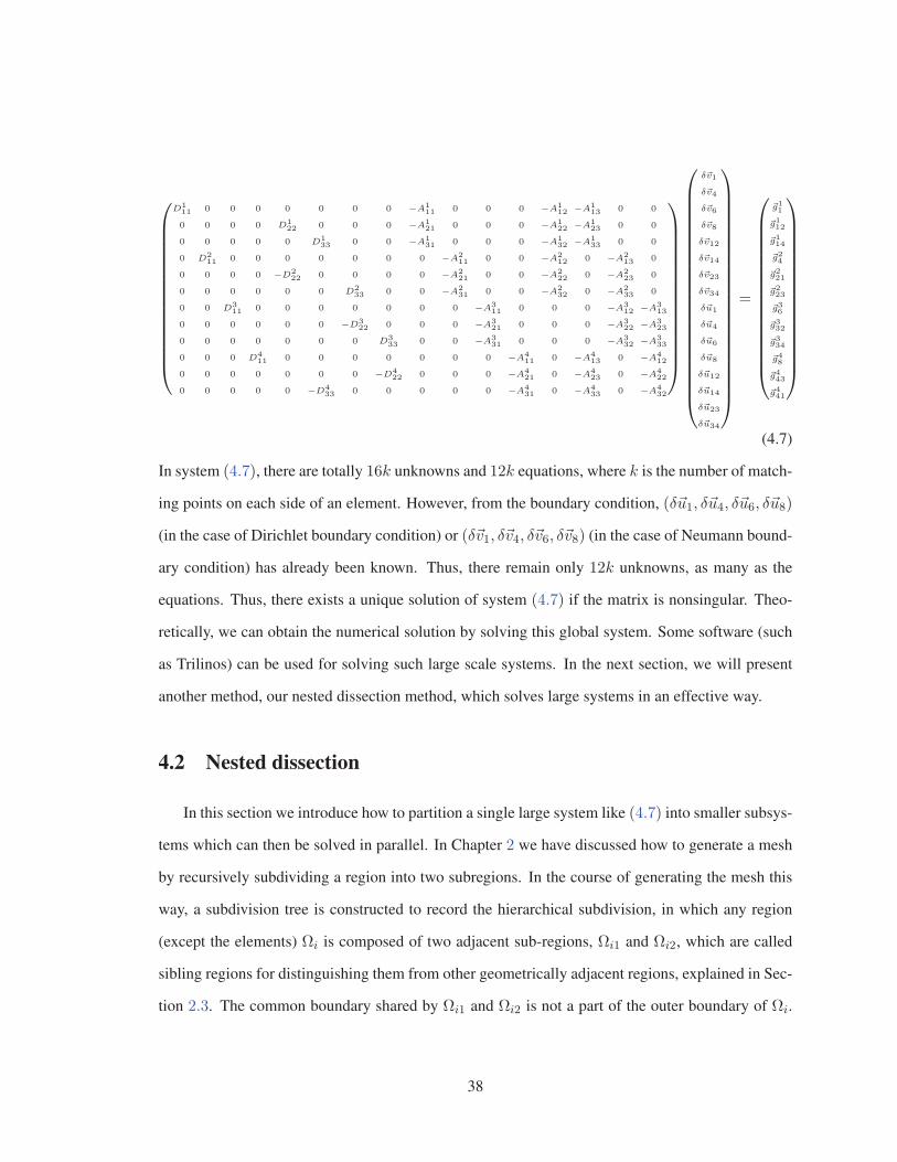
⎛⎜⎜⎜⎜⎜⎜⎜⎜⎜⎜⎜⎜⎜⎜⎝
D111 0 0 0 0 0 0 0 −A1
11 0 0 0 −A112 −A1
13 0 0
0 0 0 0 D122 0 0 0 −A1
21 0 0 0 −A122 −A1
23 0 0
0 0 0 0 0 D133 0 0 −A1
31 0 0 0 −A132 −A1
33 0 0
0 D211 0 0 0 0 0 0 0 −A2
11 0 0 −A212 0 −A2
13 0
0 0 0 0 −D222 0 0 0 0 −A2
21 0 0 −A222 0 −A2
23 0
0 0 0 0 0 0 D233 0 0 −A2
31 0 0 −A232 0 −A2
33 0
0 0 D311 0 0 0 0 0 0 0 −A3
11 0 0 0 −A312 −A3
13
0 0 0 0 0 0 −D322 0 0 0 −A3
21 0 0 0 −A322 −A3
23
0 0 0 0 0 0 0 D333 0 0 −A3
31 0 0 0 −A332 −A3
33
0 0 0 D411 0 0 0 0 0 0 0 −A4
11 0 −A413 0 −A4
12
0 0 0 0 0 0 0 −D422 0 0 0 −A4
21 0 −A423 0 −A4
22
0 0 0 0 0 −D433 0 0 0 0 0 −A4
31 0 −A433 0 −A4
32
⎞⎟⎟⎟⎟⎟⎟⎟⎟⎟⎟⎟⎟⎟⎟⎠
⎛⎜⎜⎜⎜⎜⎜⎜⎜⎜⎜⎜⎜⎜⎜⎜⎜⎜⎜⎜⎜⎜⎝
δ�v1
δ�v4
δ�v6
δ�v8
δ�v12
δ�v14
δ�v23
δ�v34
δ�u1
δ�u4
δ�u6
δ�u8
δ�u12
δ�u14
δ�u23
δ�u34
⎞⎟⎟⎟⎟⎟⎟⎟⎟⎟⎟⎟⎟⎟⎟⎟⎟⎟⎟⎟⎟⎟⎠
=
⎛⎜⎜⎜⎜⎜⎜⎜⎜⎜⎜⎜⎜⎜⎜⎜⎝
�g11
�g112
�g114
�g24
�g221
�g223
�g36
�g332
�g334
�g48
�g443
�g441
⎞⎟⎟⎟⎟⎟⎟⎟⎟⎟⎟⎟⎟⎟⎟⎟⎠
(4.7)
In system (4.7), there are totally 16k unknowns and 12k equations, where k is the number of match-
ing points on each side of an element. However, from the boundary condition, (δ�u1, δ�u4, δ�u6, δ�u8)
(in the case of Dirichlet boundary condition) or (δ�v1, δ�v4, δ�v6, δ�v8) (in the case of Neumann bound-
ary condition) has already been known. Thus, there remain only 12k unknowns, as many as the
equations. Thus, there exists a unique solution of system (4.7) if the matrix is nonsingular. Theo-
retically, we can obtain the numerical solution by solving this global system. Some software (such
as Trilinos) can be used for solving such large scale systems. In the next section, we will present
another method, our nested dissection method, which solves large systems in an effective way.
4.2 Nested dissection
In this section we introduce how to partition a single large system like (4.7) into smaller subsys-
tems which can then be solved in parallel. In Chapter 2 we have discussed how to generate a mesh
by recursively subdividing a region into two subregions. In the course of generating the mesh this
way, a subdivision tree is constructed to record the hierarchical subdivision, in which any region
(except the elements) Ωi is composed of two adjacent sub-regions, Ωi1 and Ωi2, which are called
sibling regions for distinguishing them from other geometrically adjacent regions, explained in Sec-
tion 2.3. The common boundary shared by Ωi1 and Ωi2 is not a part of the outer boundary of Ωi.
38
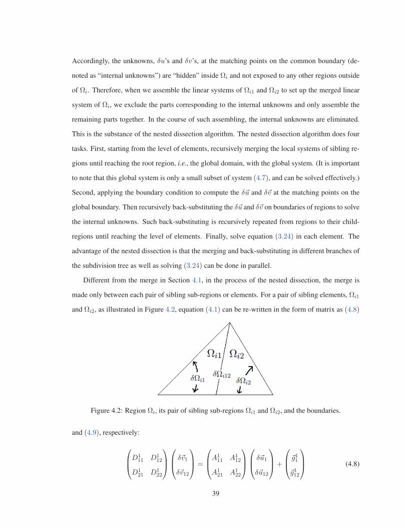
Accordingly, the unknowns, δu’s and δv’s, at the matching points on the common boundary (de-
noted as “internal unknowns”) are “hidden” inside Ωi and not exposed to any other regions outside
of Ωi. Therefore, when we assemble the linear systems of Ωi1 and Ωi2 to set up the merged linear
system of Ωi, we exclude the parts corresponding to the internal unknowns and only assemble the
remaining parts together. In the course of such assembling, the internal unknowns are eliminated.
This is the substance of the nested dissection algorithm. The nested dissection algorithm does four
tasks. First, starting from the level of elements, recursively merging the local systems of sibling re-
gions until reaching the root region, i.e., the global domain, with the global system. (It is important
to note that this global system is only a small subset of system (4.7), and can be solved effectively.)
Second, applying the boundary condition to compute the δ�u and δ�v at the matching points on the
global boundary. Then recursively back-substituting the δ�u and δ�v on boundaries of regions to solve
the internal unknowns. Such back-substituting is recursively repeated from regions to their child-
regions until reaching the level of elements. Finally, solve equation (3.24) in each element. The
advantage of the nested dissection is that the merging and back-substituting in different branches of
the subdivision tree as well as solving (3.24) can be done in parallel.
Different from the merge in Section 4.1, in the process of the nested dissection, the merge is
made only between each pair of sibling sub-regions or elements. For a pair of sibling elements, Ωi1
and Ωi2, as illustrated in Figure 4.2, equation (4.1) can be re-written in the form of matrix as (4.8)
Figure 4.2: Region Ωi, its pair of sibling sub-regions Ωi1 and Ωi2, and the boundaries.
and (4.9), respectively:
⎛⎜⎝D1
11 D112
D121 D1
22
⎞⎟⎠
⎛⎜⎝ δ�v1
δ�v12
⎞⎟⎠ =
⎛⎜⎝A1
11 A112
A121 A1
22
⎞⎟⎠
⎛⎜⎝ δ�u1
δ�u12
⎞⎟⎠+
⎛⎜⎝�g11
�g112
⎞⎟⎠ (4.8)
39

⎛⎜⎝D2
11 D212
D221 D2
22
⎞⎟⎠
⎛⎜⎝ δ�v2
δ�v21
⎞⎟⎠ =
⎛⎜⎝A2
11 A212
A221 A2
22
⎞⎟⎠
⎛⎜⎝ δ�u2
δ�u21
⎞⎟⎠+
⎛⎜⎝�g22
�g221
⎞⎟⎠ (4.9)
where δ�v12, δ�u12, δ�v21, and δ�u21 are on the common edge, δΩi12, shared by Ωi1 and Ωi2. The other
δ�v’s and δ�u’s are on δΩi1 and δΩi2, respectively. From continuity equation (3.11) and (3.12), we
must have
(a) δ�u12 = δ�u21 (b) δ�v12 = −δ�v21 , (4.10)
Merging system (4.8) and (4.9) together, and taking equation (4.10) into consideration, we obtain
the following equation:
⎛⎜⎜⎜⎜⎜⎜⎜⎝
D122 −A1
22 D121 −A1
21 0 0
−D222 −A2
22 0 0 D221 −A2
21
D112 −A1
12 D111 −A1
11 0 0
−D212 −A2
12 0 0 D211 −A2
11
⎞⎟⎟⎟⎟⎟⎟⎟⎠
⎛⎜⎜⎜⎜⎜⎜⎜⎜⎜⎜⎜⎜⎜⎜⎝
δ�v12
δ�u12
δ�v1
δ�u1
δ�v2
δ�u2
⎞⎟⎟⎟⎟⎟⎟⎟⎟⎟⎟⎟⎟⎟⎟⎠
=
⎛⎜⎜⎜⎜⎜⎜⎜⎝
�g112
�g221
�g11
�g22
⎞⎟⎟⎟⎟⎟⎟⎟⎠
, (4.11)
We use scaled row pivoting. Scaled pivoting is a variation of the partial pivoting strategy. In
this approach, the algorithm selects as the pivot element the entry that is largest relative to the
entries in its row. This strategy is desirable when entries’ large differences in magnitude lead to the
propagation of round-off error. Scaled pivoting should be used in a system where a row’s entries
vary greatly in magnitude [38]. The system in our collocation method is of this case. Using scaled
40

row pivoting, apply incomplete Gaussian Elimination to system (4.11) to get the following system:
⎛⎜⎜⎜⎜⎜⎜⎜⎝
∗ ∗ # # # #
0 ∗ # # # #
0 0 × × × ×0 0 × × × ×
⎞⎟⎟⎟⎟⎟⎟⎟⎠
⎛⎜⎜⎜⎜⎜⎜⎜⎜⎜⎜⎜⎜⎜⎜⎝
δ�v12
δ�u12
δ�v1
δ�u1
δ�v2
δ�u2
⎞⎟⎟⎟⎟⎟⎟⎟⎟⎟⎟⎟⎟⎟⎟⎠
=
⎛⎜⎜⎜⎜⎜⎜⎜⎝
h12
h21
h1
h2
⎞⎟⎟⎟⎟⎟⎟⎟⎠
(4.12)
System (4.12) indicates that, for any region, if the (�v1, �u1, �v2, �u2)T on its boundary has been known,
then the value of (�v12, �u12)T on the border shared by its two child-regions can then be solved.
Furthermore, from system (4.12), we can extract
⎛⎜⎝× × × ×× × × ×
⎞⎟⎠
⎛⎜⎜⎜⎜⎜⎜⎜⎝
δ�v1
δ�u1
δ�v2
δ�u2
⎞⎟⎟⎟⎟⎟⎟⎟⎠
=
⎛⎜⎝h1
h2
⎞⎟⎠ , (4.13)
which has the same form of system (4.8) or (4.9). Thus, when merging this region with its sibling
region, we can repeat the above process. We repeat such merging recursively until we reach the en-
tire domain Ω. For the system (4.11) at the level of the entire domain Ω, we will be able to compute
the (δ�v1, δ�v2)T or (δ�u1, δ�u2)T from the given Neumann boundary condition or Dirichlet boundary
condition, respectively. Then we back-substitute it into the subsystem (4.12) to solve (δ�u1, δ�u2)T
or (δ�v1, δ�v2)T . We have now (δ�v1, δ�u1, δ�v2, δ�u2)T which we can back-substitute into system (4.11)
to obtain (δ�v1, δ�v2)T . Repeat such back-substitution recursively until the level immediately above
the individual elements. Then in each element, we solve equation (3.24) to obtain the δ�c of the
element. The steps of the piecewise case are listed below:• Apply the initial condition to the �u, �v, and �c of all elements.
• Loop over all elements. For each element, compute Φ (3.13) and RΦ (3.14).
• Loop of time integration. At each time step, do the following tasks:
◦ The Newton iteration for solving equation (3.24), until sufficiently converged.In each round of the Newton iteration:
41

∗ Loop over all elements. For each element:· Compute LΦ (3.19). —– (1)
· Solve (3.28) to get matrices A and B. —– (2)
· Compute �rN (3.16), �ru, and �rv (3.21).· Construct the local system (3.26) of the element.
(These computations can be done simultaneously in multiple elements.)∗ Loop of recursively merging elements/child-regions, as shown from (4.8) to (4.13),
until the entire domain is reached; (This can be done in parallel.)∗ Apply boundary conditions to the δ�u or δ�v on the boundary, then solve the global
system (4.12) for the internal unknown δ�u and δ�v. —(3)
∗ Loop of recursively solving the local system (4.12) of sub-regions for the internalunknown δ�u and δ�v until reaching the individual elements. (This can be done inparallel.)
∗ Loop over all elements; for each element:· Solve equation (3.24) (with current LΦ, δ�u, �ru, �rN ) to get current δ�c;· �c+ = δ�c, �u+ = δ�u, �v+ = δ�v;
(This can be done in parallel.)◦ Save the current �u, �v, and �c for the use as initial values and uk−1 when computing �rN
(3.16), (3.8) at next time step.
• End.
The steps marked with (1), (2), and (3) in the above sequence have the same comments as given in
Section 3.5.
4.3 Generalization of the nested dissection
In Section 2.2 and 2.3, we have introduced generating meshes by recursively subdividing re-
gions into pairs of sub-regions with single straight lines. Then we proceed the nested dissection;
that is, recursively merging the pairs of sub-regions until finally reaching the entire domain. How-
ever, the nested dissection algorithm is not limited to being used with the meshes generated by
subdivision. In fact, the nested dissection algorithm can be used with any meshes as long as we
can find a way to construct a hierarchy of recursive subdivisions on the top of its elements, no mat-
ter how the elements have been generated or whether the border-line between each pair of sibling
sub-regions is a straight lines or polyline. In Section 2.5, we have described how to establish such
subdivision hierarchy (i.e., subdivision tree) from existing elements which have been generated by
no matter which triangulation and refinement algorithms. Figure 4.3 ∼ 4.6 illustrate some examples
of subdivision constructed from the existing elements. Except for the bisection in Figure 4.3, the
regions in all the other figures are subdivided by generally shaped polylines. We can recursively
42

construct such subdivisions in sub-regions until the level of elements. In the subdivisions shown in
the figures, each border-line, no matter split into how many segments, can be stored and manipu-
lated as a single chain of the edges of the elements. Our current data structure does support such
edge chains; therefore, it potentially supports this generalized application of the nested dissection
procedure.
Figure 4.3: A region bisected into a pairof equal subregions by a single straightline.
Figure 4.4: A region subdivided intoa pair of irregularly-shaped and -sizedsubregions by a polyline.
Figure 4.5: A region subdivided into apair of nested subregions by a closedpolyline.
Figure 4.6: A region subdivided into apair of subregions by 2 separate poly-lines.
4.4 Complexity analysis
To estimate the complexity, we count the number of arithmetic operations and memory transfers
involved in Newton iteration and time integration. We do not count one-time computations.
For each element, we need to compute matrix LΦ (3.18), which is of dimension (m+ n)×m.
Thus, there are (m + n) × m items to compute, each of which involves arithmetic operations
and/or complex mathematical functions, such as sin(), log(), exp(), etc., depending on the PDEs in
43

question. For the complexity brought by arithmetic operations, we count only the multiplications
and divisions, as done in [20]. For the complexity caused by the mathematical function f(), which
is a ”black box” to us, we can only denote it as C(f), where the ”C()” stands for complexity. Also
taking the number of elements, k, into consideration, the total complexity of the step is
O(k(m+ n)2C(f)) (4.14)
arithmetic operations.
For each element, computing �rN (3.16), �ru, and �rv (3.21) causes O((m+ n)C(f)) operations.
In comparison to the complexity of (4.14), this step can be ignored.
For each element, to perform a LU-decomposition on the system (3.28) to solve matrix A and
B, we need 13((m+ n)2 − 1)(m+ n) arithmetic operations [20], where m,n represent the number
of collocation and matching points, respectively. Thus, for all the k elements, we need
O(k(m+ n)3) (4.15)
arithmetic operations.
Now we estimate the work load in the merged regions at all levels in the bisection tree. The
work load includes copying matrix blocks of the child regions to the matrices of the merged re-
gions, the Gaussian Elimination and back-substitution for solving its internal (δ�v, δ�u)T , and the
Gaussian Elimination and back-substitution for solving the outer (δ�v, δ�u)T on its boundary. The
complexity of Gaussian Elimination is O(N3), where the N is the size of the matrix. Thus, we
need to determine the values of N . From Equation (4.8) and (4.9), we know that the size of the
merged matrix in (4.11) depends only on the sizes of matrices A1 and A2. According to Equation
(3.25), the size of matrix Aj depends only on the number of the matching points on its boundary.
Thus, the size of the merged matrix has nothing to do with the number of collocation points. We
roughly estimate that any merged region at level (i + 1) has on average 43ni matching points on
its boundary, where ni is the number of matching points on the boundary of either its child-region
at level i. Elements are at level 0. We also estimate the merged matrix of any merged region at
level (i + 1) is of the size of 43ni × 4
3ni, i.e., N = 43ni. Thus, for a square domain with a mesh
44
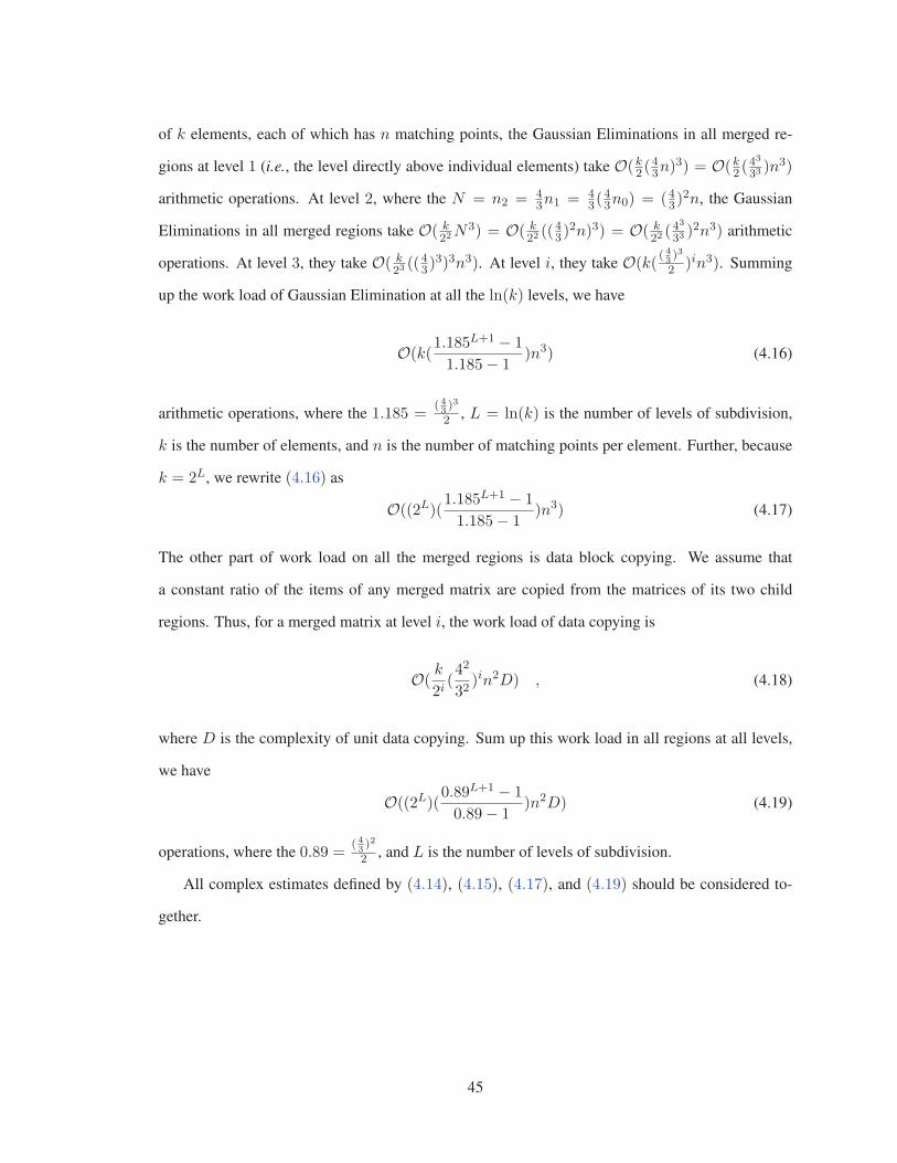
of k elements, each of which has n matching points, the Gaussian Eliminations in all merged re-
gions at level 1 (i.e., the level directly above individual elements) take O(k2 (43n)
3) = O(k2 (43
33)n3)
arithmetic operations. At level 2, where the N = n2 = 43n1 = 4
3(43n0) = (43)
2n, the Gaussian
Eliminations in all merged regions take O( k22N3) = O( k
22((43)
2n)3) = O( k22(4
3
33)2n3) arithmetic
operations. At level 3, they take O( k23((43)
3)3n3). At level i, they take O(k(( 43)3
2 )in3). Summing
up the work load of Gaussian Elimination at all the ln(k) levels, we have
O(k(1.185L+1 − 1
1.185− 1)n3) (4.16)
arithmetic operations, where the 1.185 =( 43)3
2 , L = ln(k) is the number of levels of subdivision,
k is the number of elements, and n is the number of matching points per element. Further, because
k = 2L, we rewrite (4.16) as
O((2L)(1.185L+1 − 1
1.185− 1)n3) (4.17)
The other part of work load on all the merged regions is data block copying. We assume that
a constant ratio of the items of any merged matrix are copied from the matrices of its two child
regions. Thus, for a merged matrix at level i, the work load of data copying is
O(k
2i(42
32)in2D) , (4.18)
where D is the complexity of unit data copying. Sum up this work load in all regions at all levels,
we have
O((2L)(0.89L+1 − 1
0.89− 1)n2D) (4.19)
operations, where the 0.89 =( 43)2
2 , and L is the number of levels of subdivision.
All complex estimates defined by (4.14), (4.15), (4.17), and (4.19) should be considered to-
gether.
45

Chapter 5
Implementation
The collocation method is an effective algorithm, which brings high accuracy solutions with
fewer elements. The basic simplicity of the collocation procedure, also makes programming of the
method reasonably straightforward [51]. On the other hand, in our collocation method, manipula-
tion of matrices leads to complexity of programming and adds overhead to the performance of our
collocation solver. Stability, accuracy, and performance rely on robust and efficient implementation
of the software prototype. There have already been some collocation method software packages in
practical use for BVP, such as the widely used AUTO[56] for continuation and bifurcation problems
in ODEs, ColSys for Boundary-Value ODEs [51], CONTENT[52], MatCont[53][54], and DDE-
Biftool[55] for ODEs, PDEs, and Bifurcation analysis. Additionally, Sharifi has implemented his
software prototype for linear / nonlinear elliptic PDEs, which relied on square meshes[17]. Qiang
Zheng has developed a prototype based on triangular meshes for linear (parabolic) PDEs. In this
thesis, we went one step further to implement a prototype which works in generally shaped do-
mains, discretized with triangular meshes, and for nonlinear parabolic PDEs. In this chapter we will
describe in detail the architecture of the software, its data structures, algorithms, and performance
consideration.
46

5.1 Overview of the prototype implementation
Our implementation of the collocation method in this thesis is a prototype, used for demonstrat-
ing a generalization of this method to nonlinear BVPs in irregularly shaped domains with triangular
adaptive meshes. The prototype is expected to achieve the following design goals:
(1) Most importantly, getting solutions with high accuracy, as shown in Chapter 6.
(2) Supporting multi-threading for parallel computation, which could improve performance. We
have actually implemented the multi-threading in the current prototype and seen a significant
acceleration of the computations.
(3) As the ”icing on the cake”, supporting dynamical adaptive mesh generation (see Section 2.1 )
at runtime (i.e., in the course of time integration of the solver), which requires
(3.1) Any element can be further subdivided at runtime for sufficient accuracy in it.
(3.2) Any pair of sibling elements can be merged into one element at runtime if enough ac-
curacy can be achieved with fewer elements. This functionality is necessary for keeping
the number of elements minimized when solving some time-dependent problems where
the solution surfaces change with time and, as a result, subdivision in some regions
would become no longer necessary as time passes by.
(3.3) For (3.1) or (3.2), vertices, edges, and elements must be created or deleted at runtime,
the values of u, v, and p at the related matching points and collocation points must be
re-evaluated, and the matrices Φ and RΦ, defined by (3.13) and (3.14), respectively,
must be re-computed.
We have already implemented the adaptive mesh refinement as a separate functionality for
examining our error estimator, refinement algorithm (i.e., Rivara algorithm), and the underly-
ing data structure supporting dynamically adding or removing vertices, edges, and elements.
We have succeeded in this aspect. However, integrating the mesh refinement into the solver at
runtime involves many elaborate programming details, which are less significant for the main
purpose of this thesis, i.e., for showing that the collocation method is feasible for nonlinear
47
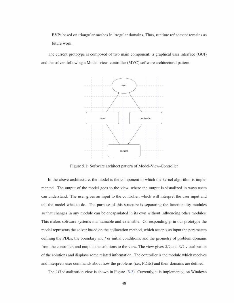
BVPs based on triangular meshes in irregular domains. Thus, runtime refinement remains as
future work.
The current prototype is composed of two main component: a graphical user interface (GUI)
and the solver, following a Model–view–controller (MVC) software architectural pattern.
model
user
view controller
Figure 5.1: Software architect pattern of Model-View-Controller
In the above architecture, the model is the component in which the kernel algorithm is imple-
mented. The output of the model goes to the view, where the output is visualized in ways users
can understand. The user gives an input to the controller, which will interpret the user input and
tell the model what to do. The purpose of this structure is separating the functionality modules
so that changes in any module can be encapsulated in its own without influencing other modules.
This makes software systems maintainable and extensible. Correspondingly, in our prototype the
model represents the solver based on the collocation method, which accepts as input the parameters
defining the PDEs, the boundary and / or initial conditions, and the geometry of problem domains
from the controller, and outputs the solutions to the view. The view gives 2D and 3D visualization
of the solutions and displays some related information. The controller is the module which receives
and interprets user commands about how the problems (i.e., PDEs) and their domains are defined.
The 2D visualization view is shown in Figure (5.2). Currently, it is implemented on Windows
48

platforms with GDI (Microsoft Windows graphics device interface ) and MFC (Microsoft Funda-
mental C++); however, if needed, it can be adapted to any other GUI frameworks on any OS. This
view is not only used for visualization, but also a user interface (UI) through which users can define
the vertices of problem domains simply by clicking mouse.
The view also includes 3D visualization of the solutions, as shown in Figure (5.3). It is an stand-
alone web-based cross-platform application, implemented by ourselves. It imports the solution
description files yielded by the model (i.e., the collocation solver), interprets the content of the files,
and renders the solution surfaces in real time. The details of our implementation of 3D visualization
and the related technologies is explained in Chapter 7.
The controller of the current prototype is a simple dialog box, in Figure (5.4), through which
users can select any one of the predefined test PDEs together with the necessary parameters. For
simplicity, we predefine the test PDEs and hard-code them in the controller. For practical use, we
need to design and implement a mechanism which expresses various PDEs in general forms and a
parser which interprets the forms and thereby constructs the context for solving the specific PDEs.
Figure 5.2: View: 2D visualization ofsolutions
Figure 5.3: View: 3D visualization ofsolutions
49

Figure 5.4: Controller: parameters and selection of test PDEs
5.2 Work flow for solving a PDE
Here we explain the work flow (as shown in Figure 5.5) of our collocation method (i.e., the
model in Figure 5.1). The first step is triangulation, as described in Section 2.2. The result of
triangulation is a group of triangle sub-regions, each of which can already be used as an element
because it is triangle. However, for getting certain levels of accuracy, some elements need to be
refined (see Section 2.1). The refinement step is repeated; in each loop, all the elements are scanned
one-by-one to check whether any of them should be further refined; if yes, refine it; if there is no
element to further refine, exit the repetition and go to next step. The next step is the iteration of
time integration marked with 1 in Figure 5.5. At each time step t, first, the numerical solution
(i.e., the values of piecewise polynomials) at time (t−1) must be set as the initial guess for Newton
iteration at time t. The Newton iteration is marked with 3 in Figure 5.5. The nested dissection
discussed in Chapter 4 is executed in each loop of 3 . In the simplest case where we solve PDEs
in the whole domain as a single element without subdividing it, and therefore no subdivision tree or
nested dissection would be involved, the 1 and 2 as a whole would be the procedure described in
Section 3.5. Constructing and traversing the subdivision tree will be discussed in detail a little after
in this section.
Note also the extended time integration iteration 2 , which includes the step of mesh refinement.
This is the unimplemented dynamical adaptive mesh refinement into the solver, mentioned at point
(3) in Section 5.1. For the dynamical adaptive mesh refinement, the dashed parts in the figure
should also be included for merging any pairs of elements in which the accuracy is more than
enough. In addition, after the dynamical refinement or merging, numerical solutions (i.e., the values
of piecewise polynomials) at time (t− 1) must be re-evaluated at the new collocation and matching
points; this would be done at the step of ”set/save the solution at time step (t-1)”.
50

user input:selected PDE,params, region
vertices, ...
triangulation of domain
mesh refinement(Rivara algorithm)
any elementto be refined?
merge the over-refinedsibling elements
any elementover-refined?
Apply Initial Condition
set/save the solutionat time step (t-1)
go bottom-up subdi-vision tree; merge
the matrices;
apply the boundarycondition at root node;
go top-down sub-division tree;
back-substitute;
not enoughconverged in
anyelements?
continue timeintegration?
output solution
1
2
3
yes
no
yes
no
yesno
yes
no
Figure 5.5: Work flow of the solver based on the collocation method
51

1
2 3
4 5 6 7
8 9 10 11 14 15
16 17 28 29
58 59
Figure 5.6: The subdivision tree
Now, we consider the subdivision tree shown in Figure 5.6. The triangle leaves of the tree are
elements. For our collocation method, the elements are triangular, so it is intuitive to represent the
elements with triangles. The red directional curves represent the pointers linking preceding elements
to their following elements, constructing a linked list, which is the result of mesh refinement. The
other nodes in the tree are merged nodes. Both elements and merged nodes are nodes, derived from
the same base class CNode. The two nodes generated by subdividing a node are child or sibling
nodes; the subdivided node is the parent node. As explained in Chapter 4, the matrix of a parent
node is generated by merging the matrices of its child nodes. By illustrating the merged nodes with
dashed instead of solid circles, we indicate that those nodes and the tree did not exist before the
first time step; the nodes must be dynamically created and the tree must be built up on-the-fly from
the current list of elements. Furthermore, if 2 is implemented, the elements would change at each
time step, so the merged nodes and the tree would have to be changed accordingly at each time step.
The process of constructing the subdivision tree is described below:
(1) The recursive subdivision operations (including domain triangulation, mesh generation, and
mesh refinement) finally generates a linked list of elements, as illustrated by the red curves in
5.6. In the course of the subdivision, we always follow an essential rule to keep the order in
which the elements are linked one after another; that is, in the current linked list, we replace
the subdivided element with the two new sibling elements, with the left brother pointing to
52

the right brother.
(2) Each node (an element or a merged node) had a subdivision ID, as shown the numbers in Figure
5.6, generated by
parentId× 2 + 0|1 ,
where parendId is the subdivision ID of its parent node. If the current node is the left child,
+0; for right child, +1. Thus, from the subdivision IDs, it is easy to recognize whether two
nodes are sibling or not.
(3) Prepare an empty stack;
(4) Set the first element in the linked list as the current node, go through all the elements in the list
and repeat the following operations:
(4.1) Check whether the current node is the brother of the top-most node (merged or element)
in the stack; if no, push the current element into the stack; if yes, do (4.2);
(4.2) Pop the top-most node out of the stack, merge it with the current node; as the result,
create a new merged node and parent-child relation; set this merged node as the current
node; then, do (4.1);
(4.3) Push the current node into the stack; move to the next element in the linked list, set it
as the current node, and do (4.1). If there is no more element in the list, it means the
whole subdivision tree has been built up, and the top-most and unique node in the stack
is the root node of the tree.
The subdivision tree can be built up one time and not rebuilt or changed any more if we do not
implement the solver as 2 ; however, the operations of merging the matrices have to be done in
each loop of 3 because the matrices change. More than 60% of the time is cost for the merge. The
algorithm itself, our data structure, and our implementation described above support multi-threading
for the operations of the merge. As shown in 5.6, we mark the elements with two colors to indicate
two threads used to do the merging in parallel. In general, more than two threads can be used.
There should also be synchronization for the threads. We have implemented multi-threading in this
53
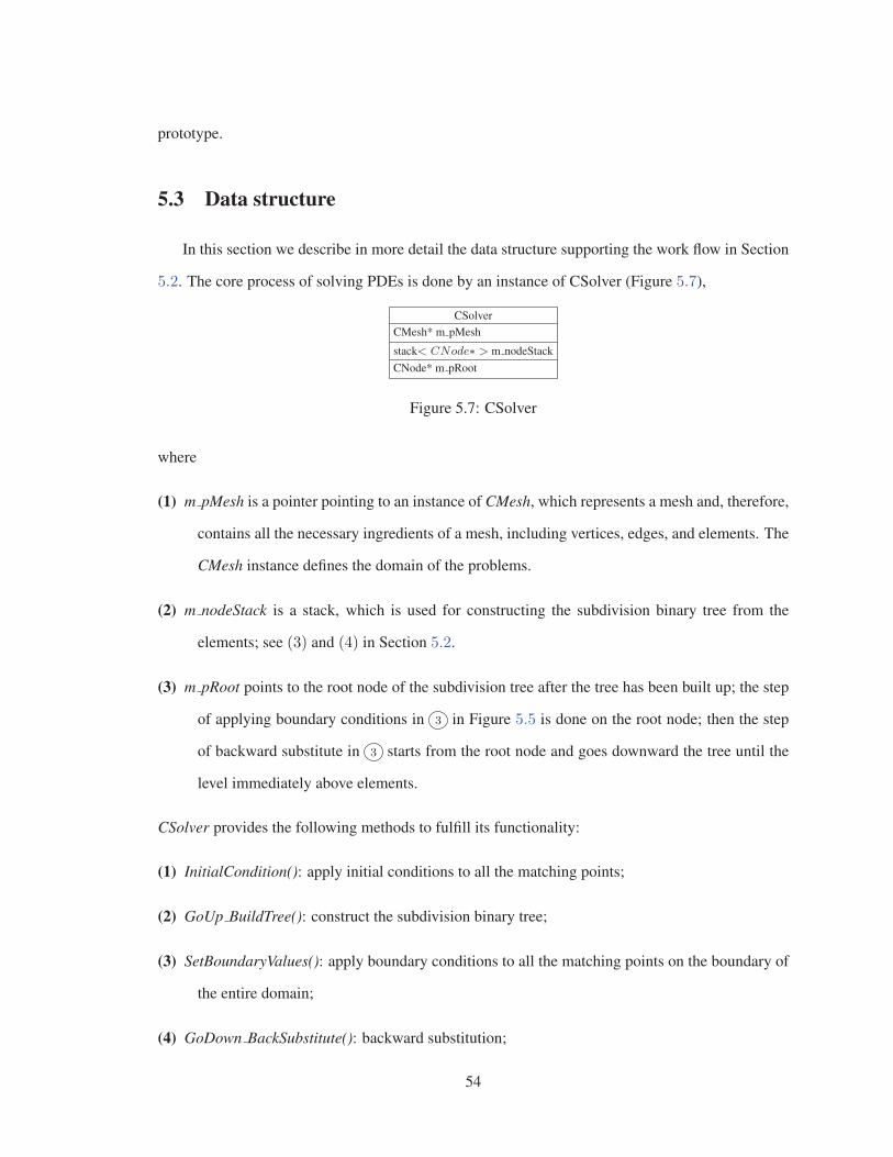
prototype.
5.3 Data structure
In this section we describe in more detail the data structure supporting the work flow in Section
5.2. The core process of solving PDEs is done by an instance of CSolver (Figure 5.7),
CSolverCMesh* m pMesh
stack< CNode∗ > m nodeStackCNode* m pRoot
Figure 5.7: CSolver
where
(1) m pMesh is a pointer pointing to an instance of CMesh, which represents a mesh and, therefore,
contains all the necessary ingredients of a mesh, including vertices, edges, and elements. The
CMesh instance defines the domain of the problems.
(2) m nodeStack is a stack, which is used for constructing the subdivision binary tree from the
elements; see (3) and (4) in Section 5.2.
(3) m pRoot points to the root node of the subdivision tree after the tree has been built up; the step
of applying boundary conditions in 3 in Figure 5.5 is done on the root node; then the step
of backward substitute in 3 starts from the root node and goes downward the tree until the
level immediately above elements.
CSolver provides the following methods to fulfill its functionality:
(1) InitialCondition(): apply initial conditions to all the matching points;
(2) GoUp BuildTree(): construct the subdivision binary tree;
(3) SetBoundaryValues(): apply boundary conditions to all the matching points on the boundary of
the entire domain;
(4) GoDown BackSubstitute(): backward substitution;
54

(5) SaveSolutionOnBoundary(): save numerical solution (i.e.,�u in 3.21 ) at matching points on
boundary for applying Boundary Conditions (B.C) to compute δ�u in 3.26;
(6) SaveLastPolynomialValAtColloPoints(): save current polynomial values (equivalent to the uk−1
in 3.7) at collocation points for use in next time step;
CMesh represents a mesh, so it contains all the necessary ingredients of a mesh, including vertices,
edges, and elements, but not including the merged regions. We will call CMesh or instance of
CMesh simply as mesh in any context where there is no ambiguity.
CMeshint m VerticeNumint m EdgeNum
int m ElementNumCVertex *m pVerticeLst head
CEdge *m pEdgeLst head
CElement *m pElementLst
CElement *m pCurrElmt
v1 v2 . . . vn−1 vn null
s1 s2 . . . sk null
e1 e2 . . . em null
Figure 5.8: Container CMesh contains all mesh information: vertices, edges, and elements.
In the mesh, we need containers to accommodate the vertices, edges, and elements. We choose
a linked list (as shown in Figure 5.8) rather than an array for the consideration of supporting dy-
namical mesh at runtime (see Section 2.1 and (3) in Section 5.1). When further subdivision is
done in an element for runtime mesh adaptation (Section 2.1), new elements together with new
edges and vertices will be created and added into the corresponding containers. Furthermore, the
new elements which, as a whole, take the place of the original subdivided element, must inherit its
neighborhood with the preceding and following elements in the element container. For an array,
keeping such neighborhood means physically inserting the new elements onto the position of the
original element, which requires physically moving all the following elements to make room for the
new elements. This is not acceptable in our situation. When adding new edges, similar conditions
55
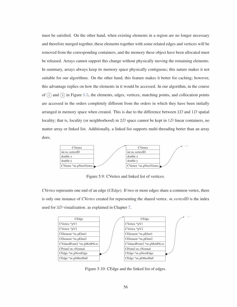
must be satisfied. On the other hand, when existing elements in a region are no longer necessary
and therefore merged together, these elements together with some related edges and vertices will be
removed from the corresponding containers, and the memory these object have been allocated must
be released. Arrays cannot support this change without physically moving the remaining elements.
In summary, arrays always keep its memory space physically contiguous; this nature makes it not
suitable for our algorithms. On the other hand, this feature makes it better for caching; however,
this advantage replies on how the elements in it would be accessed. In our algorithm, in the course
of 1 and 3 in Figure 5.5, the elements, edges, vertices, matching points, and collocation points
are accessed in the orders completely different from the orders in which they have been initially
arranged in memory space when created. This is due to the difference between 2D and 1D spatial
locality; that is, locality (or neighborhood) in 2D space cannot be kept in 1D linear containers, no
matter array or linked list. Additionally, a linked list supports multi-threading better than an array
does.
CVertexint m vertexIDdouble xdouble y
CVertex *m pNextVertex
CVertexint m vertexIDdouble xdouble y
CVertex *m pNextVertex
. . .
Figure 5.9: CVertex and linked list of vertices.
CVertex represents one end of an edge (CEdge). If two or more edges share a common vertex, there
is only one instance of CVertex created for representing the shared vertex. m vertexID is the index
used for 3D visualization. as explained in Chapter 7.
CEdge
CVertex *pV1
CVertex *pV2
CElement *m pElmt1
CElement *m pElmt2
CValuedPoint2 *m pMchPtLst;
CPoint2 m vNormalCEdge *m pNextEdge
CEdge *m pOtherHalf
CEdge
CVertex *pV1
CVertex *pV2
CElement *m pElmt1
CElement *m pElmt2
CValuedPoint2 *m pMchPtLst;
CPoint2 m vNormalCEdge *m pNextEdge
CEdge *m pOtherHalf
. . .
Figure 5.10: CEdge and the linked list of edges.
56

CEdge represents a side of an element. For a merged region (CMergedRegion), which is at least
composed of two elements, some of its sides may be conposed of a sequence of collinear edges
linked in series. Each of such multi-edged sides is represented by a chain of CEdge objects (i.e.,
edge chain), linked by m pOtherHalf, and identified by header and tail. We will describe in more
detail how to build up this type of chains when discussing CMergedRegion. For now, it is enough
to know that an edge chain is a multi-edged side of a merged region. pV1 and pV2 point to the
two vertices; m pElmt1 and m pElmt2 points to the two elements sharing this edge; m pMchPtLst
points to a list of CPoint2D objects, representing the matching points on this edge; m vNormal is a
unit vector perpendicular the edge; specified positive direction, this vector will be the outwards unit
vector, ηi, in (3.12); m pOtherHalf has the following two uses. First, marking pending edges in the
course of mesh generation. When an edge is still pending (defined in Section 2.3), m pOtherHalf
points the new edge separated from it; when it is no longer pending, its m pOtherHalf is set to null.
Secondly, as mentioned previously, constructing edge chains of merged regions.
CElement represents elements. An element is a special type of node, so CElement derives from
base class CNode, as shown in Figure 5.11. In the figure, the gray part represents CNode, which
defines the essential geometrical features and parent-child relationship of a region; the light part
is the extra attributes of CElement, which correspond to the matrices and vectors mentioned in
Section 3.2 and 3.3; in addition, CElement also defines operations on these attributes, among which
the following:
(1) GenerateMat CopyToMerged(. . . ) : locate collocation points, generate the matrices, compute
matrix A and vector �g in (3.26), and copy them into the sub-matrices, m pMat Triangles,
m pMat 2, m pMat All 0, and m pMat DA of CMergedRegion. We will explain it in more
detail when discussing CMergedRegion;
(2) LocateColloPoints( ) : called by GenerateMat CopyToMerged(. . . ) to place collocation points;
(3) InitMatrices(. . . ) : called by GenerateMat CopyToMerged(. . . ) to create and compute the
matrices in Section 3.2 and 3.3;
A pair of sibling elements have the same parent merged region, as shown in 5.11.
57

CElement : CNodeint m subTree ID == 2n+ 0
int m Edge num == 3
CEdge** m ppEdge
CNode* m pChld[0] == null
CNode* m pChld[1]
CNode* m pMother
int m dSignOfDeltaV
byte m Status
CPolynomial m objPolynomial
CPoint2D* m pColloPtLst
VectorXd* m pVectC
double* m prU
double* m prN
MatrixXd* m pMat RF
MatrixXd* m pMat negA B Transposed
double* m pMat negFai Data
double* m pMat RF Data
double* m pMat L Data
double* m pVect P collo LastT
VectorXd* m pU
VectorXd* m pV
bool m bIsConverged
CElement : CNodeint m subTree ID == 2n+ 1
int m Edge num == 3
CEdge** m ppEdge
CNode* m pChld[0] == null
CNode* m pChld[1]
CNode* m pMother
int m dSignOfDeltaV
byte m Status
CPolynomial m objPolynomial
CPoint2D* m pColloPtLst
VectorXd* m pVectC
double* m prU
double* m prN
MatrixXd* m pMat RF
MatrixXd* m pMat negA B Transposed
double* m pMat negFai Data
double* m pMat RF Data
double* m pMat L Data
double* m pVect P collo LastT
VectorXd* m pU
VectorXd* m pV
bool m bIsConverged
CMergedRegion
int m subTree ID == nint m Edge num � 3
CNode* m pChld[0]
CNode* m pChld[1]. . .
Next CElement
Figure 5.11: CElement and the linked list of elements.
58
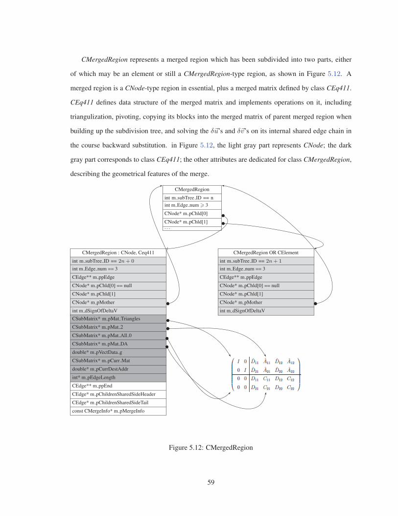
CMergedRegion represents a merged region which has been subdivided into two parts, either
of which may be an element or still a CMergedRegion-type region, as shown in Figure 5.12. A
merged region is a CNode-type region in essential, plus a merged matrix defined by class CEq411.
CEq411 defines data structure of the merged matrix and implements operations on it, including
triangulization, pivoting, copying its blocks into the merged matrix of parent merged region when
building up the subdivision tree, and solving the δ�u’s and δ�v’s on its internal shared edge chain in
the course backward substitution. in Figure 5.12, the light gray part represents CNode; the dark
gray part corresponds to class CEq411; the other attributes are dedicated for class CMergedRegion,
describing the geometrical features of the merge.
CMergedRegion : CNode, Ceq411
int m subTree ID == 2n+ 0
int m Edge num == 3
CEdge** m ppEdge
CNode* m pChld[0] == null
CNode* m pChld[1]
CNode* m pMother
int m dSignOfDeltaV
CSubMatrix* m pMat Triangles
CSubMatrix* m pMat 2
CSubMatrix* m pMat All 0
CSubMatrix* m pMat DA
double* m pVectData g
CSubMatrix* m pCurr Mat
double* m pCurrDestAddr
int* m pEdgeLength
CEdge** m ppEnd
CEdge* m pChildrenSharedSideHeader
CEdge* m pChildrenSharedSideTail
const CMergeInfo* m pMergeInfo
CMergedRegion
int m subTree ID == nint m Edge num � 3
CNode* m pChld[0]
CNode* m pChld[1]. . .
CMergedRegion OR CElement
int m subTree ID == 2n+ 1
int m Edge num == 3
CEdge** m ppEdge
CNode* m pChld[0] == null
CNode* m pChld[1]
CNode* m pMother
int m dSignOfDeltaV
Figure 5.12: CMergedRegion
59

The merging of elements and merged regions is illustrated in Figure 5.13:
Figure 5.13: Merging of elements and merged regions
The layout in Figure 5.13 is the result of 3 levels of subdivision. The i is the index of the edges; the
numbers inside the elements are m subTree ID’s, which are used for recognizing sibling nodes.
The red circles and blue triangles visualize the pairs of sibling nodes. Now, look at the blue triangle
marked as No.2. It is a merged region, so it is an instance of class CMergedRegion; we name it as
region2. It has 3 sides, each of which is an edge chain. One side is composed of edge edge 13 and
4 ; this edge chain is defined the following way:
(1) region2.m ppEdge[0] → edge 4 ;
(2) region2.m ppEnd[0] → edge 13 ;
(3) edge 4 .m pOtherHalf → edge 13 ;
(4) in this simple subdivision scenario, there is no more edge in the chain following edge 13 , so
edge 13 .m pOtherHalf == null;
The other two sides of region2 have also such structure; that is:
{region2.m ppEdge[1] → edge 3 ;
60
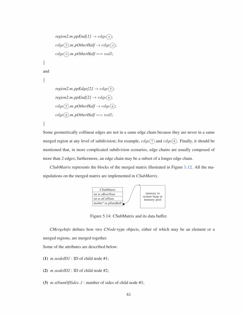
region2.m ppEnd[1] → edge 15 ;
edge 3 .m pOtherHalf → edge 15 ;
edge 15 .m pOtherHalf == null;
}and
{region2.m ppEdge[2] → edge 5 ;
region2.m ppEnd[2] → edge 6 ;
edge 5 .m pOtherHalf → edge 6 ;
edge 6 .m pOtherHalf == null;
}Some geometrically collinear edges are not in a same edge chain because they are never in a same
merged region at any level of subdivision; for example, edge 7 and edge 8 . Finally, it should be
mentioned that, in more complicated subdivision scenarios, edge chains are usually composed of
more than 2 edges; furthermore, an edge chain may be a subset of a longer edge chain.
CSubMatrix represents the blocks of the merged matrix illustrated in Figure 5.12. All the ma-
nipulations on the merged matrix are implemented in CSubMatrix.
CSubMatrixint m nRowNumint m nColNumdouble* m pDataBuff
memory insystem heap ormemory pool
Figure 5.14: CSubMatrix and its data buffer.
CMergeInfo defines how two CNode-type objects, either of which may be an element or a
merged regions, are merged together.
Some of the attributes are described below:
(1) m nodeID1 : ID of child node #1;
(2) m nodeID2 : ID of child node #2;
(3) m nNumOfSides 1 : number of sides of child node #1;
61

CMergeInfo
unsigned int m nodeID1
unsigned int m nodeID2
unsigned int m nNumOfSides 1
unsigned int m nNumOfSides 2
unsigned int m nNumOfSides Merged
unsigned int m nMatchPntNumber
int m nLength SharedEdge
int m nLength Merged Head
int m nLength Merged Tail
int m nRowsFirstChildint* m p Child Merged
int stackMem[0]. . .
int stackMem[8]
memory insystem heap ormemory pool
Figure 5.15: CMergeInfo
(4) m nNumOfSides 2 : number of sides of child node #2;
(5) m nNumOfSides Merged : number of sides merged region;
(6) m nLength SharedEdge : number of edges in the edge chain shared by child node #1 and #2;
(7) m nLength Merged Head : in the merged edge chain, how many edges are from child node #1;
(8) m nLength Merged Tail : in the merged edge chain, how many edges are from child node #2;
(9) m nRowsFirstChild : in the merged matrix, how many rows correspond to child node #1;
(10) m p Child Merged : among all the sides of child #1 and #2, which are shared, which are
merged;
These attributes tell how many rows and columns the merged matrix and its sub-matrices contain
and how to arrange the blocks copied from child #1 and #2.
Finally, relationship of the classes are shown in Diagram 5.16. . . .
5.4 Optimization
In the course of the nested dissection, many operations can be done in parallel as shown in
Section 4.2. The most substantial optimization of performance is to implement the parallelism.
62
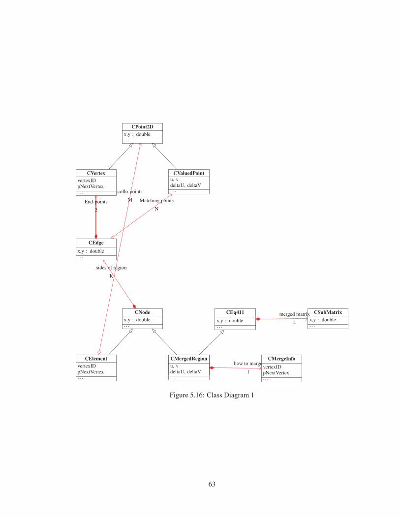
CPoint2D
x,y : double. . .
CVertex
vertexIDpNextVertex. . .
CValuedPoint
u, vdeltaU, deltaV. . .
CEdge
x,y : double. . .
CNode
x,y : double. . .
CEq411
x,y : double. . .
CElement
vertexIDpNextVertex. . .
CHidden
u, vdeltaU, deltaV
CMergedRegion
u, vdeltaU, deltaV. . .
CSubMatrix
x,y : double. . .
CMergeInfo
vertexIDpNextVertex. . .
collo-points
MEnd-points
2
Matching points
N
sides of region
K
merged matrix
4
how to marge
1
Figure 5.16: Class Diagram 1
63

CMesh
vertex Numedge Numelement Numcurr element. . .. . .
CVertex. . .. . .
CEdge. . .. . .
CElement. . .. . .
CSolver. . .. . .
CNode. . .. . .
CPolynomial. . .. . .
<<interface>>IBasis
. . .
. . .
CPhai. . .. . .
chain of elements1..*
chain of edges
1..*
chain of vertices1..*
containexactly 1
B-Trees1..*
linear combination..
..basis
linear combination..
..basis
linear combination..
..basis
Figure 5.17: Class Diagram 2
64

There exist various frameworks and application programming interfaces (APIs) supporting parallel
computing, for example: OpenMP, Message Passing Interface (MPI), OpenCL, CUDA, and mul-
tithreading. Multi-threading would be easiest way for harnessing the power of multi-core CPUs.
We have implemented the multi-threading at the steps of computing the matrices of all the elements
and merging the local systems. Our tests indicate that these steps are the bottleneck of perfor-
mance; therefore, we only make these steps executed in parallel. Additionally, integrating the mesh
refinement with the time evolution would bring excellent effect of mesh-moving when solving time-
dependent PDEs. For these improvements, the data structure will still be based on linked list because
it supports effectively adding or removing nodes. On the other hand, a linked list takes more time
for accessing individual nodes and it breaks locality of reference, which is critically important for
CPU cache. Thus, customized memory management system is needed for solving these problems.
We leave the optimization for future work.
5.5 The Eigen library
When implementing our collocation method, we make use of Eigen library for solving and
checking singularity of the essential and basic linear systems, like the following:
M�x = �b,
where M is matrix. We need not implement this kinds of computation; reinventing a wheel is
meaningless. Eigen is an existing wheel ready for use.
Eigen is a C++ template library for linear algebra: matrices, vectors, numerical solvers, and related
algorithms.[57] It is fast, easy to integrate into C++ projects, and cross platform. It is well supported
and documented, and has plenty of learning resources and a large user group. Its official website is
eigen.tuxfamily.org.
Additionally, although we base the very basic algebraic computations on the Eigen library, we
have made our implementation of the algorithms independent with this library. The benefit of doing
so is that we would easily migrate to any other more advanced 3rdparty libraries if necessary.
Suppose we find a library which can make use of the enormous computation power of GPU’s, we
65

would easily replace the current library with that one simply by modifying some source code to
follow the interface specification of that library.
66

Chapter 6
Numerical Results
In this chapter we use sample parabolic PDEs to test the accuracy and convergence of our
collocation method. The sample PDEs include nonlinear and linear parabolic problems with or
without stationary solutions. By means of these tests, we determine the key factors influencing
the accuracy of the numerical solutions. For our collocation method, there are no well-established
analytical error estimates.
6.1 Factors determining accuracy and convergence
Accuracy and convergence of the collocation method are affected by mesh size, the number of
collocation points and matching points, and the locations of the collocation points and matching
points. If the mesh size is very small, local and relative coordinate must be used; otherwise, the
collocation method may not converge. The accuracy of time-dependent PDEs is also affected by the
size of time step.
6.1.1 Mesh size
We need to provide error estimates for our algorithm with respect to different mesh sizes. This
will make it possible to evaluate our numerical results. However, based on our knowledge, there is
no well-established analytical theory which formulates general relations between the size of meshes
with triangular elements and the order of accuracy. Even so, there exist some theoretical analysis
67
given for some special cases. In [21], Yinnian He and Weiwei Sun have given optimal error estimate
for a low-order nonconforming spline collocation method on triangular mesh. Their theoretical
analysis is limited to a low-order collocation method based on triangular elements with (nc, nm) =
(1, 3), which means 1 collocation point at center and a total of 3 matching points on the 3 edges.
We include this case into our tests and we will evaluate the errors according to the error estimate
given by the theorems in section 3 of [21]. A high-order case using a triangular elements with
(nc, nm) = (6, 9) is tested in [22] without mathematical analysis. It is implied in [21] that an error
analysis for high-order collocation methods remains under investigation.
An error analysis for higher order cases is given by Theorem 3.5 in [22]. However, it is based
on rectangular meshes and cannot be extended to triangular meshes [21]. This theorem states that
‖u− uh‖1 ≤ Ch3,
where the u and uh are the exact and numerical solution, respectively, h is the mesh size, and ‖ · ‖1is the energy norm, defined as
‖u− uh‖1 =(∫
Ω|∇u−∇uh|2dxdy
)1/2.
The above error analysis in Section III of [22] is based on the equivalence between the noncon-
forming spline collocation method and a special high-order finite difference method in the case of
a rectangular mesh on a rectangular domain [21][22]. After the collocation system is reduced to an
equivalent finite difference system, the truncation error and energy error are derived based on the
finite difference system.
A less precise but more general error estimate is given by Lemma 3.9.1 on Page 43 in Section
3.4 of Sharifi’s thesis [17]. The principle is identical to the one mentioned above [22]; that is,
converting the collocation system into an equivalent finite difference system, which is formulated
by (3.5) in the case of an ODE with 1D mesh, or (5.3) in the case of PDE with 2D mesh in [17],
and then apply Taylor expansions to the finite difference system to prove the truncation error is of
order O(h2), where h is the mesh size. The conversion from a collocation system to an equivalent
finite difference system is not limited to a rectangular mesh. It is also applicable to a triangular
68

mesh, as proved in Theorem 1 in [20]. Thus, for a collocation system with triangular mesh, the
truncation error given in Section 3.4 of Hamid’s thesis [17] still holds.
All the above analytical error estimates are derived from linear collocation systems. They will
also be valid for our nonlinear collocation system because, by the collocation method, we have
linearized the nonlinear PDE (and constructed a Newton iteration system) and then, by local elim-
ination, reduced the original collocation system into a finite difference system, as formulated by
(6.14) in [17]:
Dδv = Aδu+ g ,
which is in the same form of the (3.5) in [22] and (5.3) in [21] as discussed above. Therefore, the
error analysis for nonlinear collocation systems follows the same principle.
6.1.2 The number of collocation points and matching points
Within some limits, increasing the number of collocation points in each element can make PDEs
better satisfied by local polynomials; increasing the number of matching points can bring better
continuity between neighboring elements. Therefore, more accurate solutions can be obtained by
appropriately increasing the numbers of collocation points and matching points. This will be shown
by the test results in Section 6.3. However, if the numbers exceed the limits, the collocation method
tends to become singular and fail to converge.
Furthermore, in some schemes of matching points and collocation points, neither the number of
matching points nor that of collocation points is large, but the difference between the two numbers
is large. For example, 3 matching points (i.e., 1 per edge) with 7 collocation points per element, or
12 matching points with less than 3 collocation points. In these cases, matrix (Φ | LΦ) will easily
become non-invertible. This type of singularity was explained at the end of Section 3.3 by Equation
(3.29), (3.30), and (3.31), with geometrical significance. Here, we enumerate more examples of
this type of singularity in Figure 6.1− 6.4.
69
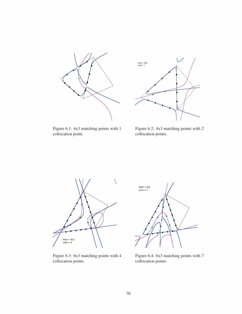
Figure 6.1: 4x3 matching points with 1collocation point.
Figure 6.2: 4x3 matching points with 2collocation points.
Figure 6.3: 6x3 matching points with 4collocation points.
Figure 6.4: 6x3 matching points with 7collocation points.
70

6.1.3 Location of collocation points and matching points
The location of collocation and matching points strongly influence accuracy. This means that,
without computational overhead, which is an inevitable consequence of increasing the number of
collocation and matching points or granularity of mesh, we can get higher accuracy. Out test results
show that, in some cases, higher order of accuracy can be obtained from fewer but well located
matching points and collocation points. Furthermore, because slightly adjusting the locations usu-
ally result in small change of accuracy, this method is stable. In most cases, the highest accuracy
and order of convergence can be obtained when we take the Gauss points on each side of elements
as the location of matching points and, at the same time, certain special collocation points inside the
elements as collocation points. The Gauss points will be described in more detail in 6.1.4. Our test
results clearly show that this rule of thumb holds for all tested PDEs and for all mesh sizes. On the
other hand, badly located collocation and matching points may cause singularity or divergence.
6.1.4 Templates of collocation and matching points
We refer to the layout of collocation and matching points as templates. A template describes
the numbers of collocation and matching points per element and how they are located. We need to
determine templates of matching and collocation points which bring stable numerical results with
high order of accuracy and convergence rate. For the matching points, their number can be selected
from 1 to 4 per edge, and they may be evenly distributed or at Gauss points on each element edge.
The definition of Gauss points is shown in Figure 6.5. For collocation points, their number can be
selected from 1 to 7 per element, and their locations are controlled by parameters. The scheme for
positioning collocation points is illustrated in Figure 6.6. We categorize the collocation points of
each element into 3 groups. Group 1 has only one collocation points which is at the center of gravity
of the element. Group 2 has 3 collocation points, located on the sections between pi′s and the center
of gravity in Figure 6.6. Their locations on the sections are controlled by parameter P defined as
below
P =2Lzi
Lpi
,
71

Figure 6.5: Locations of Gauss points. Column n is the number of Gauss points. Column i is theindex of the Gauss points. Column ti is the location of the Gauss points. Column ci is the weight,which is unrelated to our collocation method. (This is TABLE-12.2 of [26])
Figure 6.6: Location of collocation points in a triangular element
72

where Lzi represents the distance by which collocation point zi is away from the center of gravity,
and Lpi is the distance between pi and the center of gravity. For example, P = 1.0 means that
all of the Group-2 collocation points are located at the mid-points of their sections. The bigger the
value of P is, the further the Group-2 collocation points are located away from the center of gravity.
Group 3 has also 3 collocation points, located on the sections between qi′s and the center of gravity
in Figure 6.6, and controlled by parameter Q defined as
Q =2Szi
Lqi
,
where Szi represents how far Group-3 collocation point zi is away from the center of gravity, and
Lqi is the distance between qi and the center of gravity.
The notation for templates is as follows:
(nc, nm[G][; (P,Q)]) ,
where nc and nm represent the number of collocation and matching points of each element, respec-
tively; the presence of G means the matching points are located at Gauss point, and the absence
of G implies the matching points are evenly arranged on each edge of elements; P and Q are the
parameters controlling locations of the collocation points, as defined above. For templates with
nc = 1, P or Q is unnecessary. For templates with nc = 2, 3, or4, only P is needed, and if P is not
given explicitly, it takes its default value 1.0. For templates with nc = 5, 6, or7, P and Q are both
necessary, and their default values are 1.0.
Some examples are given below:
(1) (1, 3): 1 collocation point and 3 (i.e., 1 per edge) matching points for each element.
(2) (6, 9G; (1.45, 1.35)): 6 collocation points at the specified locations, with 3 matching points per
edge at Gauss points.
(3) (7, 12; (1.5, 1.25)): 7 collocation points at the specified locations, with 4 matching points evenly
distributed on each edge.
The templates of collocation points tested in our research include (but not limited to) the following:
73

(1) (7, nm; (P = 1.5, Q = 1.25)).
(2) (4, nm; 1.25).
(3) (3, nm; 1.0), which corresponds to the 3-quadrature-point Area coordinate given in TABLE I
on Page 6 of [22]. (See Figure 6.7)
(4) (4, nm; 0.8), which corresponds to the 4-quadrature-point Area coordinate given in TABLE I
on Page 6 of [22]. (See Figure 6.7)
(5) (6, nm; (P = 1.45, Q = 1.35)), which corresponds to the 6-quadrature-point Area coordinate
given in TABLE I on Page 6 of [22]. (See Figure 6.7)
Figure 6.7: A copy of the TABLE I from [22].
6.2 Initial condition and time integration
For solving a parabolic PDE using our collocation method, we need to specify an initial con-
dition, written as u(x, y, 0) or u|t0 , from which to start time integration. At each time step ti of
the time integration, the Newton iteration is executed to find the solution at ti. (For details, see the
steps listed at the end of Section 4.2.) We first compute �u, �v, and �c of every element from the initial
condition u(x, y, 0), and take them as the initial guess for the Newton iteration at t1. We always
take the result �u, �v, and �c at ti−1 as the initial guess for the Newton iteration at ti. The Newton
iteration may be globally convergent, which means that it always converges to a solution for any
74

initial guess, or locally convergent if it only converges to a solution from an initial guess sufficiently
close to the solution. Having global or local convergence depends on the PDE, the time interval δt.
and/or the u(x, y, 0). There are several strategies to define the initial condition and make the initial
guess of �c, as described below:
1. If the initial condition u(x, y, 0) has been given together with the parabolic PDE, we applyu(x, y, 0) to all the collocation points and matching points in the entire domain, and chooseeither of the following methods to make the initial guess of �c :
1.1 Simply set the ci’s of all the �c ’s to 0. This arbitrary initial guess is usually not close tothe solution. We can only hope the Newton iteration has global convergence.
1.2 For each element, construct a linear system of �c based on the values of u(x, y, 0) eval-uated at the collocation points and matching points of the element. Then solve thissystem and take the solution of �c as the initial guess, which is better than an arbitraryinitial guess.
2. If we need to try various u(x, y, 0) (for detecting different stationary solution families, forexample), and the boundary condition has been given as B(x, y, t), where (x, y) ∈ δΩ, wecan choose either of the following options to define the u(x, y, 0):
2.1 Specify u(x, y, 0) = a, where a is constant. Then follow either the above 1.1 or 1.2for the initial guess of �c. The u(x, y, 0) is not necessarily equal to B(x, y, 0) at thematching points on the boundary. If the difference between the two is large, and δt isvery small, then at the first several time steps, there would be sudden changes over theelements close to the boundary.
2.2 Let u(x, y, 0) = B(x, y, 0) + bF (x, y), where (x, y) ∈ Ω, b is a coefficient for scaling,and F (x, y) is defined as any one below:
F (x, y) = x1/16(1− x)1/16y1/16(1− y)1/16 , shown in Figure 6.8(a)
F (x, y) = x1/8(1− x)1/8y1/8(1− y)1/8 , shown in Figure 6.8(b)
F (x, y) = x1/4(1− x)1/4y1/4(1− y)1/4 , shown in Figure 6.8(c)F (x, y) = 4x(1− x)y(1− y) , shown in Figure 6.8(d)
Thus, u(x, y, 0) = B(x, y, 0) on the boundary because F (x, y) = 0 there, and u(x, y, 0)is still smooth and continuous near the boundary. This feature eliminates the suddenchange near the boundary and leads to more smooth solution surfaces near the boundary.Then choose either the above 1.1 or 1.2 for initial guess of �c.
Figure 6.8: Profile of F (x, y).
75

6.3 Example PDEs for numerical experiments
6.3.1 A linear parabolic PDE with a stationary solution
Linear PDEs can be considered as special cases of nonlinear PDEs. It is well known that the
application of Newton iteration to a linear problem converges in one iteration step. However, for
ill-conditioned linear problems, more than one iteration steps correspond to residual correction.
This test PDE is from [20] with modified initial condition and an extra parameter a, which is
used for scaling the height of the solution surface. If a = 1.0, this test PDE is identical to the PDE
given in [20], so we can use the results provided in [20] as a reference for evaluating the accuracy
of our method. At the end of this test, we will compare the accuracy of the numerical solutions of
PDE 6.1 obtained by our collocation method to the results in [20].
The PDE is defined as the following:
∂u
∂t= Δu− 2ae(x+y), (x, y) ∈ Ω ⊂ R2
u(x, y, 0) = 0, for (x, y) ∈ Ω
u(x, y, t) = ae(x+y), for (x, y) ∈ ∂Ω .
(6.1)
We start the time integration of the PDE from the initial condition, u(x, y, 0) = 0. A stable station-
ary state is reached by the time integration in about 3 time units, as shown in Figure 6.14. At the
stationary state, ∂u∂t = 0, thus the parabolic PDE is equivalent to the elliptic PDE below:
0 = Δu− 2ae(x+y) , (6.2)
the exact solution of which is
u(x, y, t) = ae(x+y) . (6.3)
Therefore the stationary solution of PDE (6.1) must be (6.3). For evaluating the accuracy of our
collocation method, we first start the time integration of PDE (6.1) with a = 1.0 until reaching the
stationary state. Then we evaluate the polynomial values at matching points and compare them to
the corresponding values of (6.3). Because the initial condition is different from the stationary
76

Figure 6.9: The solution at t = 0.004,observed from below Figure 6.10: The solution at t = 0.008
Figure 6.11: The solution at t = 0.02 Figure 6.12: The solution at t = 0.05
Figure 6.13: Solution at t = 0.1Figure 6.14: A near stationary solutionwhen t � 3.0.
77

solution, we see the transient solutions evolving during the time integration. The transient solutions
of PDE (6.1) with a = 1/8 are visualized in Figure 6.9 ∼ 6.13. We then test other initial conditions
such as
u(x, y, 0) = ae(x+y) + 10x(1− x)y(1− y), for (x, y) ∈ Ω . (6.4)
This initial condition is consistent with the boundary condition. As the result, at each time step, the
transient solutions are smooth surfaces. Starting from the initial condition (6.4), we go through
Figure 6.15: At t = 0, the initial condi-tion (6.4) with a = 1/8.
Figure 6.16: The transient solution att = 0.05
Figure 6.17: The transient solution att = 0.1
Figure 6.18: The transient solution att � 1.0
a different time evolution, as shown in Figure 6.15 ∼ 6.18, but finally reach the same stationary
solution in Figure 6.14.
78
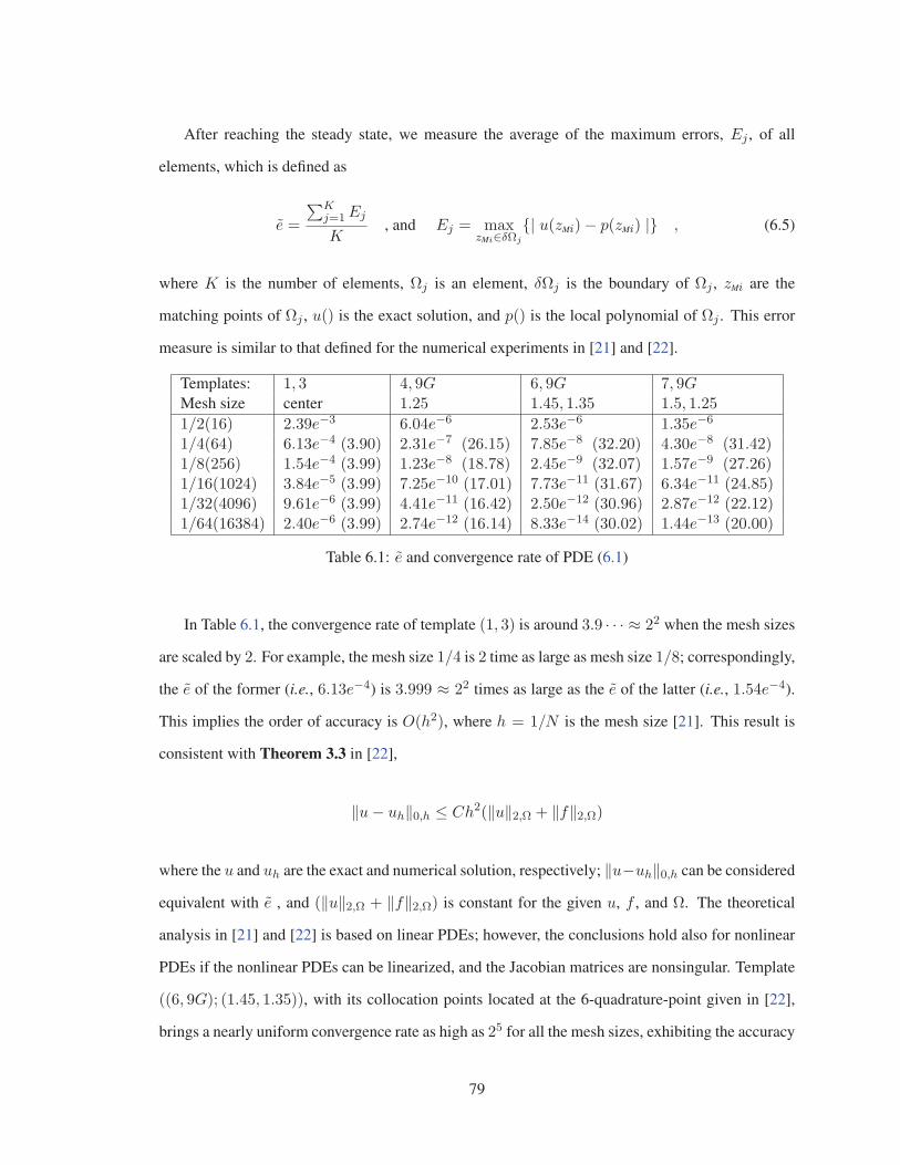
After reaching the steady state, we measure the average of the maximum errors, Ej , of all
elements, which is defined as
e =
∑Kj=1Ej
K, and Ej = max
zMi∈δΩj
{| u(zMi)− p(zMi) |} , (6.5)
where K is the number of elements, Ωj is an element, δΩj is the boundary of Ωj , zMi are the
matching points of Ωj , u() is the exact solution, and p() is the local polynomial of Ωj . This error
measure is similar to that defined for the numerical experiments in [21] and [22].
Templates: 1, 3 4, 9G 6, 9G 7, 9GMesh size center 1.25 1.45, 1.35 1.5, 1.25
1/2(16) 2.39e−3 6.04e−6 2.53e−6 1.35e−6
1/4(64) 6.13e−4 (3.90) 2.31e−7 (26.15) 7.85e−8 (32.20) 4.30e−8 (31.42)1/8(256) 1.54e−4 (3.99) 1.23e−8 (18.78) 2.45e−9 (32.07) 1.57e−9 (27.26)1/16(1024) 3.84e−5 (3.99) 7.25e−10 (17.01) 7.73e−11 (31.67) 6.34e−11 (24.85)1/32(4096) 9.61e−6 (3.99) 4.41e−11 (16.42) 2.50e−12 (30.96) 2.87e−12 (22.12)1/64(16384) 2.40e−6 (3.99) 2.74e−12 (16.14) 8.33e−14 (30.02) 1.44e−13 (20.00)
Table 6.1: e and convergence rate of PDE (6.1)
In Table 6.1, the convergence rate of template (1, 3) is around 3.9 · · · ≈ 22 when the mesh sizes
are scaled by 2. For example, the mesh size 1/4 is 2 time as large as mesh size 1/8; correspondingly,
the e of the former (i.e., 6.13e−4) is 3.999 ≈ 22 times as large as the e of the latter (i.e., 1.54e−4).
This implies the order of accuracy is O(h2), where h = 1/N is the mesh size [21]. This result is
consistent with Theorem 3.3 in [22],
‖u− uh‖0,h ≤ Ch2(‖u‖2,Ω + ‖f‖2,Ω)
where the u and uh are the exact and numerical solution, respectively; ‖u−uh‖0,h can be considered
equivalent with e , and (‖u‖2,Ω + ‖f‖2,Ω) is constant for the given u, f , and Ω. The theoretical
analysis in [21] and [22] is based on linear PDEs; however, the conclusions hold also for nonlinear
PDEs if the nonlinear PDEs can be linearized, and the Jacobian matrices are nonsingular. Template
((6, 9G); (1.45, 1.35)), with its collocation points located at the 6-quadrature-point given in [22],
brings a nearly uniform convergence rate as high as 25 for all the mesh sizes, exhibiting the accuracy
79
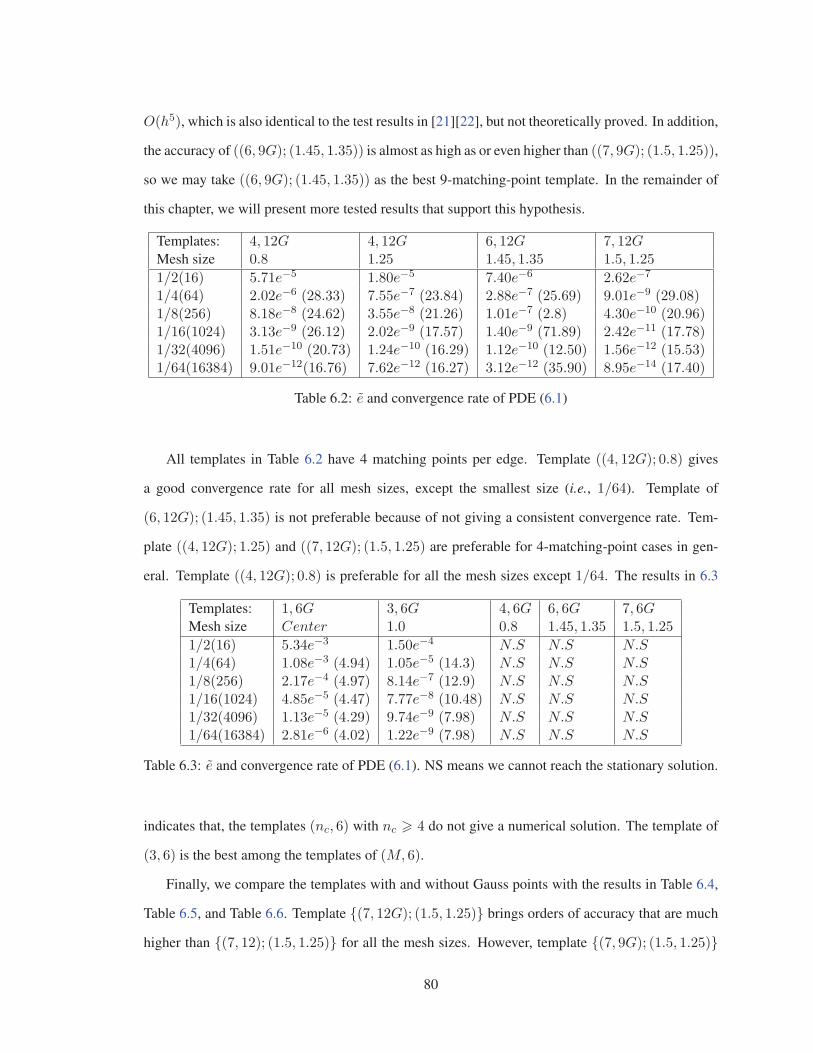
O(h5), which is also identical to the test results in [21][22], but not theoretically proved. In addition,
the accuracy of ((6, 9G); (1.45, 1.35)) is almost as high as or even higher than ((7, 9G); (1.5, 1.25)),
so we may take ((6, 9G); (1.45, 1.35)) as the best 9-matching-point template. In the remainder of
this chapter, we will present more tested results that support this hypothesis.
Templates: 4, 12G 4, 12G 6, 12G 7, 12GMesh size 0.8 1.25 1.45, 1.35 1.5, 1.25
1/2(16) 5.71e−5 1.80e−5 7.40e−6 2.62e−7
1/4(64) 2.02e−6 (28.33) 7.55e−7 (23.84) 2.88e−7 (25.69) 9.01e−9 (29.08)1/8(256) 8.18e−8 (24.62) 3.55e−8 (21.26) 1.01e−7 (2.8) 4.30e−10 (20.96)1/16(1024) 3.13e−9 (26.12) 2.02e−9 (17.57) 1.40e−9 (71.89) 2.42e−11 (17.78)1/32(4096) 1.51e−10 (20.73) 1.24e−10 (16.29) 1.12e−10 (12.50) 1.56e−12 (15.53)1/64(16384) 9.01e−12(16.76) 7.62e−12 (16.27) 3.12e−12 (35.90) 8.95e−14 (17.40)
Table 6.2: e and convergence rate of PDE (6.1)
All templates in Table 6.2 have 4 matching points per edge. Template ((4, 12G); 0.8) gives
a good convergence rate for all mesh sizes, except the smallest size (i.e., 1/64). Template of
(6, 12G); (1.45, 1.35) is not preferable because of not giving a consistent convergence rate. Tem-
plate ((4, 12G); 1.25) and ((7, 12G); (1.5, 1.25) are preferable for 4-matching-point cases in gen-
eral. Template ((4, 12G); 0.8) is preferable for all the mesh sizes except 1/64. The results in 6.3
Templates: 1, 6G 3, 6G 4, 6G 6, 6G 7, 6GMesh size Center 1.0 0.8 1.45, 1.35 1.5, 1.25
1/2(16) 5.34e−3 1.50e−4 N.S N.S N.S1/4(64) 1.08e−3 (4.94) 1.05e−5 (14.3) N.S N.S N.S1/8(256) 2.17e−4 (4.97) 8.14e−7 (12.9) N.S N.S N.S1/16(1024) 4.85e−5 (4.47) 7.77e−8 (10.48) N.S N.S N.S1/32(4096) 1.13e−5 (4.29) 9.74e−9 (7.98) N.S N.S N.S1/64(16384) 2.81e−6 (4.02) 1.22e−9 (7.98) N.S N.S N.S
Table 6.3: e and convergence rate of PDE (6.1). NS means we cannot reach the stationary solution.
indicates that, the templates (nc, 6) with nc � 4 do not give a numerical solution. The template of
(3, 6) is the best among the templates of (M, 6).
Finally, we compare the templates with and without Gauss points with the results in Table 6.4,
Table 6.5, and Table 6.6. Template {(7, 12G); (1.5, 1.25)} brings orders of accuracy that are much
higher than {(7, 12); (1.5, 1.25)} for all the mesh sizes. However, template {(7, 9G); (1.5, 1.25)}
80
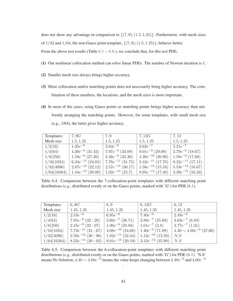
does not show any advantage in comparison to {(7, 9); (1.5, 1.25)}. Furthermore, with mesh sizes
of 1/32 and 1/64, the non-Gauss point template, {(7, 9); (1.5, 1.25)}, behaves better.
From the above test results (Table 6.1− 6.6 ), we conclude that, for this test PDE,
(1) Our nonlinear collocation method can solve linear PDEs. The number of Newton iteration is 1.
(2) Smaller mesh size always brings higher accuracy.
(3) More collocation and/or matching points does not necessarily bring higher accuracy. The com-
bination of these numbers, the locations, and the mesh sizes is more important.
(4) In most of the cases, using Gauss points as matching points brings higher accuracy than uni-
formly arranging the matching points. However, for some templates, with small mesh size
(e.g., 1/64), the latter gives higher accuracy.
Templates: 7, 9G 7, 9 7, 12G 7, 12Mesh size 1.5, 1.25 1.5, 1.25 1.5, 1.25 1.5, 1.25
1/2(16) 1.35e−6 2.64e−6 2.62e−7 5.21e−7
1/4(64) 4.30e−8 (31.42) 7.97e−8 (33.08) 9.01e−9 (29.08) 2.79e−8 (18.67)1/8(256) 1.58e−9 (27.26) 2.46e−9 (32.36) 4.30e−10 (20.96) 1.58e−9 (17.68)1/16(1024) 6.34e−11 (24.85) 7.76e−11 (31.75) 2.42e−11 (17.78) 9.22e−11 (17.11)1/32(4096) 2.87e−12 (22.12) 2.57e−12 (30.17) 1.56e−12 (15.53) 5.53e−12 (16.67)1/64(16384) 1.44e−13 (20.00) 1.02e−13 (25.7) 8.95e−14 (17.40) 3.39e−13 (16.33)
Table 6.4: Comparison between the 7-collocation-point templates with different matching pointdistributions (e.g., distributed evenly or on the Gauss points, marked with ’G’) for PDE (6.1).
Templates: 6, 9G 6, 9 6, 12G 6, 12Mesh size 1.45, 1.35 1.45, 1.35 1.45, 1.35 1.45, 1.35
1/2(16) 2.53e−6 6.95e−6 7.40e−6 2.48e−6
1/4(64) 7.85e−8 (32 : 20) 2.60e−7 (26.71) 2.88e−7 (25.69) 3.63e−7 (6.83)1/8(256) 2.45e−9 (32 : 07) 1.00e−8 (25.88) 1.01e−7 (2.8) 2.77e−7 (1.31)1/16(1024) 7.73e−11 (31 : 67) 4.08e−10 (24.60) 1.40e−9 (71.89) 4.40 ∼ 4.60e−9 (37.66)1/32(4096) 2.50e−12 (30 : 96) 1.82e−11 (22.44) 1.12e−10 (12.50) N.S1/64(16384) 8.33e−14 (30 : 02) 9.01e−13 (20.19) 3.12e−12 (35.90) N.S
Table 6.5: Comparison between the 6-collocation-point templates with different matching pointdistributions (e.g., distributed evenly or on the Gauss points, marked with ’G’) for PDE (6.1). ’N.S’means No Solution; 4.40 ∼ 4.60e−9 means the value keeps changing between 4.40e−9 and 4.60e−9
.
81
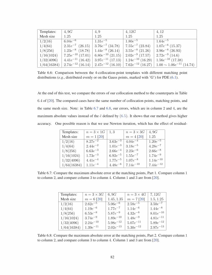
Templates: 4, 9G 4, 9 4, 12G 4, 12Mesh size 1.25 1.25 1.25 1.25
1/2(16) 6.04e−6 1.31e−5 1.80e−5 1.64e−5
1/4(64) 2.31e−7 (26.15) 3.76e−7 (34.78) 7.55e−7 (23.84) 1.07e−6 (15.37)1/8(256) 1.23e−8 (18.78) 1.44e−8 (26.14) 3.55e−8 (21.26) 3.96e−8 (26.93)1/16(1024) 7.25e−10 (17.01) 6.80e−10 (21.15) 2.02e−9 (17.57) 2.72e−9 (14.6)1/32(4096) 4.41e−11 (16.42) 3.97e−11 (17.13) 1.24e−10 (16.29) 1.56e−10 (17.38)1/64(16384) 2.74e−12 (16.14) 2.47e−12 (16.10) 7.62e−12 (16.27) 1.00 ∼ 1.06e−11 (14.74)
Table 6.6: Comparison between the 4-collocation-point templates with different matching pointdistributions (e.g., distributed evenly or on the Gauss points, marked with ’G’) for PDE (6.1).
At the end of this test, we compare the errors of our collocation method to the counterparts in Table
6.4 of [20]. The compared cases have the same number of collocation points, matching points, and
the same mesh size. Note: in Table 6.7 and 6.8, our errors, which are in column 2 and 4, are the
maximum absolute values instead of the e defined by (6.5). It shows that our method gives higher
accuracy. One possible reason is that we use Newton iteration, which has the effect of residual-
Templates: n = 3× 1G 1, 3 n = 3× 3G 4, 9GMesh size m = 1 [20] m = 4 [20] 1.25
1/2(16) 8.27e−2 3.63e−3 4.04e−4 1.20e−5
1/4(64) 2.44e−2 1.01e−3 3.18e−5 4.28e−7
1/8(256) 6.63e−3 2.66e−4 2.23e−6 2.66e−8
1/16(1024) 1.73e−3 6.92e−5 1.55e−7 1.74e−9
1/32(4096) 4.41e−4 1.77e−5 1.07e−8 1.14e−10
1/64(16384) 1.11e−4 4.48e−6 7.14e−10 7.44e−12
Table 6.7: Compare the maximum absolute error at the matching points, Part 1. Compare column 1to column 2, and compare column 3 to column 4. Column 1 and 3 are from [20].
Templates: n = 3× 3G 6, 9G n = 3× 4G 7, 12GMesh size m = 6 [20] 1.45, 1.35 m = 7 [20] 1.5, 1.25
1/2(16) 2.62e−5 5.06e−6 2.58e−5 3.50e−7
1/4(64) 1.19e−6 1.77e−7 1.14e−6 1.44e−8
1/8(256) 6.53e−8 5.87e−9 4.32e−8 8.01e−10
1/16(1024) 3.74e−9 1.89e−10 1.48e−9 4.81e−11
1/32(4096) 2.24e−10 5.98e−12 5.07e−11 5.89e−12
1/64(16384) 1.39e−11 2.02e−13 5.30e−12 2.97e−13
Table 6.8: Compare the maximum absolute error at the matching points, Part 2. Compare column 1to column 2, and compare column 3 to column 4. Column 1 and 3 are from [20].
82
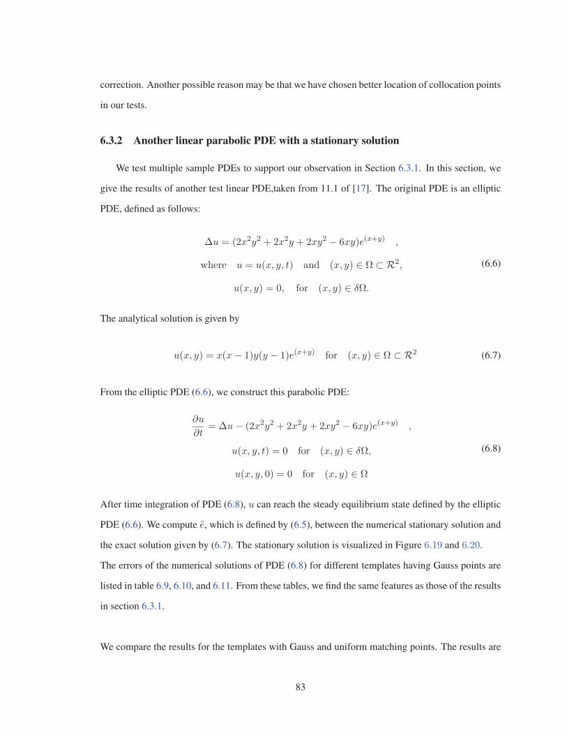
correction. Another possible reason may be that we have chosen better location of collocation points
in our tests.
6.3.2 Another linear parabolic PDE with a stationary solution
We test multiple sample PDEs to support our observation in Section 6.3.1. In this section, we
give the results of another test linear PDE,taken from 11.1 of [17]. The original PDE is an elliptic
PDE, defined as follows:
Δu = (2x2y2 + 2x2y + 2xy2 − 6xy)e(x+y) ,
where u = u(x, y, t) and (x, y) ∈ Ω ⊂ R2,
u(x, y) = 0, for (x, y) ∈ δΩ.
(6.6)
The analytical solution is given by
u(x, y) = x(x− 1)y(y − 1)e(x+y) for (x, y) ∈ Ω ⊂ R2 (6.7)
From the elliptic PDE (6.6), we construct this parabolic PDE:
∂u
∂t= Δu− (2x2y2 + 2x2y + 2xy2 − 6xy)e(x+y) ,
u(x, y, t) = 0 for (x, y) ∈ δΩ,
u(x, y, 0) = 0 for (x, y) ∈ Ω
(6.8)
After time integration of PDE (6.8), u can reach the steady equilibrium state defined by the elliptic
PDE (6.6). We compute e, which is defined by (6.5), between the numerical stationary solution and
the exact solution given by (6.7). The stationary solution is visualized in Figure 6.19 and 6.20.
The errors of the numerical solutions of PDE (6.8) for different templates having Gauss points are
listed in table 6.9, 6.10, and 6.11. From these tables, we find the same features as those of the results
in section 6.3.1.
We compare the results for the templates with Gauss and uniform matching points. The results are
83

Figure 6.19: The stationary solu-tion of PDE (6.8); center value ≈0.1699.
Figure 6.20: The stationary solution ofPDE (6.8).
Templates: 1, 3 4, 9G 6, 9G 7, 9GMesh size center 1.25 1.45, 1.35 1.5, 1.25
1/2(16) 2.93e−2 6.96e−4 3.27e−5 4.40e−5
1/4(64) 7.32e−3 (4.00) 4.45e−5 (15.65) 9.51e−7 (34.38) 1.35e−6 (32.52)1/8(256) 1.82e−3 (4.02) 2.79e−6 (15.95) 2.96e−8 (32.13) 5.01e−8 (27.02)1/16(1024) 4.56e−4 (3.99) 1.75e−7 (15.94) 9.33e−10 (31.73) 2.03e−9 (24.68)1/32(4096) 1.14e−4 (4.00) 1.09e−8 (16.06) 3.00e−11 (31.10) 9.17e−11 (22.14)1/64(16384) 2.84e−5 (4.01) 6.84e−10 (15.94) 9.91e−13 (30.27) 4.61e−12 (19.89)
Table 6.9: e and convergence rate of PDE (6.8)
Templates: 4, 12G 4, 12G 6, 12G 7, 12GMesh size 0.8 1.25 1.45, 1.35 1.5, 1.25
1/2(16) 2.48e−3 8.40e−4 3.50e−3 4.37e−5
1/4(64) 7.91e−5 (31.35) 2.71e−5 (30.99) 1.51e−4 (23.18) 1.42e−6 (30.77)1/8(256) 2.66e−6 (29.73) 2.16e−6 (12.55) 4.31e−5 (3.5) 4.60e−8 (30.87)1/16(1024) 1.35e−7 (19.70) 7.96e−8 (27.14) 4.97e−7 (86.72) 1.50e−9 (30.67)1/32(4096) 7.69e−9 (17.55) 4.79e−9 (16.63) 1.23e−8 (40.41) 5.13e−11 (29.24)1/64(16384) 4.54e−10 (16.95) 2.98e−10(16.03)∗ 5.70e−9(2.15)∗ 1.89e−12 (27.08)
Table 6.10: e and convergence rate of PDE (6.8)
Templates: 1, 6G 3, 6G 4, 6G 6, 6G 7, 6GMesh size Center 1.0 0.8 1.45, 1.35 1.5, 1.25
1/2(16) 7.41e−2 5.52e−3 N.S N.S N.S1/4(64) 1.10e−2 (6.75) 7.78e−4 (7.09) N.S N.S N.S1/8(256) 2.10e−3 (5.23) 1.02e−4 (7.63) N.S N.S N.S1/16(1024) 4.63e−4 (4.5) 1.32e−5 (7.73) N.S N.S N.S1/32(4096) 1.09e−4 (4.23) 1.67e−6 (7.9) N.S N.S N.S1/64(16384) 2.68e−5 (4.07) 2.11e−7 (7.91) N.S N.S N.S
Table 6.11: e and convergence rate of PDE (6.8)
84

in Table 6.12, 6.13, and 6.14:
Templates: 7, 9G 7, 9 7, 12G 7, 12Mesh size 1.5, 1.25 1.5, 1.25 1.5, 1.25 1.5, 1.25
1/2(16) 4.40e−5 1.30e−4 4.37e−5 5.02e−5
1/4(64) 1.35e−6 (32.52) 5.72e−6 (22.77) 1.42e−6 (30.77) 2.02e−6 (24.85)1/8(256) 5.01e−8 (27.02) 2.86e−7 (20.0) 4.60e−8 (30.87) 9.26e−8 (21.81)1/16(1024) 2.03e−9 (24.68) 1.54e−8 (18.53) 1.50e−9 (30.67) 4.78e−9 (19.37)1/32(4096) 9.17e−11 (22.14) 8.83e−10 (17.47) 5.13e−11 (29.24) 2.67e−10 (17.86)1/64(16384) 4.61e−12 (19.89) 5.26e−11 (16.79) 1.89e−12 (27.08) 1.57e−11 (16.98)
Table 6.12: Comparison between the 7-collocation-point templates with different matching pointdistributions (e.g., distributed evenly or on the Gauss points, marked with ’G’) for PDE (6.8).
Templates: 6, 9G 6, 9 6, 12G 6, 12Mesh size 1.45, 1.35 1.45, 1.35 1.45, 1.35 1.45, 1.35
1/2(16) 3.27e−5 1.57e−4 3.50e−3 8.03e−4
1/4(64) 9.51e−7 (34.38) 7.69e−6 (20.42) 1.51e−4 (23.18) 1.61e−4 (4.99)1/8(256) 2.96e−8 (32.13) 3.93e−7 (19.56) 4.31e−5 (3.5) 1.78e−4 (0.90)1/16(1024) 9.33e−10 (31.73) 2.10e−8 (18.71) 4.97e−7 (86.72) 2.78e−6 (64.08)1/32(4096) 3.00e−11 (31.10) 1.19e−9 (17.64) 1.23e−8 (40.41) NS1/64(16384) 3.85e−12 (7.8) 7.03e−11 (16.93) 5.70e−9(2.15)∗ NS
Table 6.13: Comparison between the 6-collocation-point templates with different matching pointdistributions (e.g., distributed evenly or on the Gauss points, marked with ’G’) for PDE (6.8). ’N.S’means we cannot reach the stationary solution.)
Templates: 4, 9G 4, 9 4, 12G 4, 12Mesh size 1.25 1.25 1.25 1.25
1/2(16) 6.96e−4 7.40e−4 8.40e−4 7.02e−4
1/4(64) 4.45e−5 (15.65) 4.73e−5 (15.66) 2.71e−5 (30.99) 4.58e−5 (15.33)1/8(256) 2.79e−6 (15.95) 2.97e−6 (15.92) 2.16e−6 (12.55) 1.42e−6 (32.25)1/16(1024) 1.75e−7 (15.94) 1.96e−7 (15.16) 7.96e−8 (27.14) 9.22e−8 (15.40)1/32(4096) 1.09e−8 (16.06) 1.24e−8 (15.83) 4.79e−9 (16.63) 5.57e−9 (16.55)1/64(16384) 6.84e−10 (15.94) 7.78e−10 (15.91) 2.98 ∗ e−10(16.03) 3.39e−10 (16.43)
Table 6.14: Comparison between the 4-collocation-point templates with different matching pointdistributions (e.g., distributed evenly or on the Gauss points, marked with ’G’) for PDE (6.8).
85

6.3.3 A nonlinear parabolic PDE with a stationary solution
In this section, we choose an example nonlinear parabolic PDE with known analytical stationary
solution to measure the accuracy of our collocation method. Furthermore, because the example
PDE has been appropriately constructed to simulate the Bratu problem, it has parameters, solution
families, and bifurcation point as in the Bratu problem. Thus, our experiment on this PDE is a good
warm-up for solving the real Bratu problem in the following section. The example PDE is given by
S. A. Odejide and Y. A. S. Aregbesola in [23]. They consider the solution of the Bratu problem in
2D
Δu+ λeu = 0, for (x, y) ∈ Ω ⊂ R2 (6.9)
in a way they called near exact solution, explained as the following. First, they carefully construct a
function of the form
u(x, y) = 2 ln(cosh( θ4) cosh[(x− 1
2)(y − 12)θ]
cosh[(x− 12)
θ2 ] cosh[(y − 1
2)θ2 ]) (6.10)
From this function, they construct the following Bratu-alike PDE:
0 = Δu+ λeu + f(x, y) for (x, y) ∈ Ω = [0, 1]× [0, 1] ⊂ R2 , (6.11)
where
f(x, y) =− 2θ2[(x− 1
2)2 + (y − 1
2)2][1− tanh2[(x− 1
2)(y − 1
2)θ]]
+θ2
2[1− tanh2((x− 1
2)θ
2)] +
θ2
2[1− tanh2((y − 1
2)θ
2)]
− λ(cosh( θ4) cosh((x− 1
2)(y − 12)θ)
cosh((x− 12)
θ2) cosh((y − 1
2)θ2))2 ,
(6.12)
in which θ and λ are two related parameters.
Then they force PDE (6.11) to be equivalent to the PDE of the Bratu problem (6.9) at the center of
Ω, i.e., (0.5, 0.5). This requires the following equality:
f(0.5, 0.5) = θ2 − λ cosh2(θ
4) ≡ 0,
86

Figure 6.21: The values of θ for variousvalues of λ from [23]
Figure 6.22: The values of u(0.5, 0.5)for various values of λ from [23]
which leads to
λ = (θ
cosh( θ4))2 (6.13)
Thus the parameter λ is a function of parameter θ, as shown in Figure 6.21. Figure 6.21 and 6.22
from [23]. The authors of [23] find a fold of λ at θc ≈ ±4.7987 and λc ≈ 7.02766 by solving
dλ
dθ= 0
Thus by making λ and θ satisfy equation (6.13), they make the function (6.10) satisfy the PDE of the
Bratu problem at (and only at) the center of domain Ω. Function (6.10) also has the fold with respect
to parameter λ, as show in Figure 6.22 [23], which is similar to that of the real Bratu problem.
For measuring the accuracy, we still need to do time integration from an initial condition (for
this example, the initial condition is identically 0) until reaching a stationary solution. For this
purpose, we construct the corresponding parabolic PDE from (6.11):
∂u
∂t= Δu+ λeu + f(x, y) ,
B.C : u(x, y, t) = 0 for (x, y) ∈ δΩ,
I.C : u(x, y, 0) = 0 for (x, y) ∈ Ω
(6.14)
The stationary solution must be stable; otherwise, we cannot detect it or stay on it. Thus, we need
to choose a good value of the parameter λ (in fact θ) such that the PDE has a reachable stationary
87

solution. For this purpose, we assume that we are currently just on a stationary solution, u1, and
the corresponding parameters are λ1 and θ1, which satisfy equation (6.13). For simplicity, only
consider u1(0.5, 0.5) because, at this point, PDE (6.14) reduces to a simpler PDE:
∂u
∂t= Δu+ λeu . (6.15)
Thus, we have
0 = Δu1 + λ1eu1 .
Then, choose λ2, which is close to λ1, and λ2 > λ1, at the same time, keep u = u1, so
∂u
∂t= Δu1 + λ2e
u1 > Δu1 + λ1eu1 = 0 .
Let the value of u for λ2 be u2. From Figure 6.21 and 6.22, we know that u1 < u2 if and only if
θ < θc. In this case, ∂u∂t > 0 means we are moving towards the solution u2 from our current state
u1. This implies that any deviation from the solution will get a negative feedback and be pull back
to the solution. Thus, the stationary solution is stable. On the contrary, if θ > θc, the solution is
unstable. Our accuracy test for PDE (6.11) is done with θ = 2.0 (Thus, λ ≈ 3.1458). The errors of
the numerical solutions of PDE (6.11) with the templates having Gauss matching points are listed
in Table 6.15, 6.16, and 6.17. From these tables, we find the same features as those of the preceding
test PDEs.
Templates: 1, 3 4, 9G 6, 9G 7, 9GMesh size center 0.8 1.45, 1.35 1.5, 1.25
1/2(16) 3.5870e−2 3.54e−4 1.72e−5 1.89e−5
1/4(64) 8.92e−3 (4.02) 2.31e−5 (15.32) 3.45e−7 (49.87) 4.51e−7 (41.83)1/8(256) 2.23e−3 (3.99) 1.47e−6 (15.71) 1.02e−8 (33.86) 1.83e−8 (24.62)1/16(1024) 5.57e−4 (4.00) 9.19e−8 (15.99) 3.25e−10 (31.35) 8.22e−10 (22.27)1/32(4096) 1.39e−4 (4.00) 5.75e−9 (15.997) 1.10e−11 (29.68) 4.08e−11 (20.17)1/64(16384) 3.48e−5 (4.01) 3.59e−10 (15.999) 4.04e−13 (27.12) 2.21e−12 (18.44)
Table 6.15: e and convergence rate of PDE (6.11)
We compare the results for the templates with and without Gauss matching points. The results are
88

Templates: 4, 12G 4, 12G 6, 12G 7, 12GMesh size 0.8 1.25 1.45, 1.35 1.5, 1.25
1/2(16) 1.36e−3 3.54e−4 3.14e−4 1.88e−5
1/4(64) 2.22e−5 (61.26) 6.39e−6 (55.33) 3.86e−5 (8.15) 8.32e−7 (22.54)1/8(256) 8.54e−7 (26) 2.78e−7 (22.95) 2.01e−6 ∗ (19.19) 3.44e−8 (24.17)1/16(1024) 6.97e−8 (12.25) 1.33e−8 (20.87) 4.70e−8 (42.82) 1.48e−9 (23.18)1/32(4096) 2.50e−9 (27.84) 7.82e−10 (17.06) 4.64e−7 (??) 6.88e−11 (21.57)1/64(16384) 1.27e−10 (19.74) 4.78e−11 ∗ (16.35) 2.85e−9 () 3.50e−12 (19.67)
Table 6.16: e and convergence rate of PDE (6.11)
Templates: 1, 6G 3, 6G 4, 6G 6, 6G 7, 6GMesh size Center 1.0 0.8 1.45, 1.35 1.5, 1.25
1/2(16) 6.21e−2 7.70e−3 N.S N.S N.S1/4(64) 9.12e−3 (6.81) 1.06e−3 (7.30) N.S N.S N.S1/8(256) 1.90e−3 (4.80) 1.38e−4 (7.66) N.S N.S N.S1/16(1024) 4.39e−4 (4.33) 1.77e−5 (7.80) N.S N.S N.S1/32(4096) 1.06e−4 (4.16) 2.24e−6 (7.89) N.S N.S N.S1/64(16384) 3.11e−5 (3.40) 2.81e−7 (7.95) N.S N.S N.S
Table 6.17: e and convergence rate of PDE (6.11)
in Table 6.18, 6.19, and 6.20. A solution of PDE (6.11) with parameters λ = 5.37 (θ = 3.0)
Templates: 7, 9G 7, 9 7, 12G 7, 12Mesh size 1.5, 1.25 1.5, 1.25 1.5, 1.25 1.5, 1.25
1/2(16) 1.89e−5 6.32e−5 1.88e−5 1.66e−5
1/4(64) 4.51e−7 (41.83) 1.48e−6 (42.67) 8.32e−7 (22.54) 1.23e−6 (13.54)1/8(256) 1.83e−8 (24.62) 9.11e−8 (16.26) 3.44e−8 (24.17) 5.54e−8 (22.16)1/16(1024) 8.22e−10 (22.27) 5.08e−9 (17.95) 1.48e−9 (23.18) 2.48e−9 (22.36)1/32(4096) 4.08e−11 (20.17) 2.89e−10 (17.59) 6.88e−11 (21.57) 1.19e−10 (20.88)1/64(16384) 2.21e−12 (18.44) 1.70e−11 (16.99) 3.50e−12 (19.67) 6.207∼e−12 (19.13)
Table 6.18: Comparison of the accuracy between the 7-collocation-point templates with matchingpoints at Gauss points (marked with ’G’) and those with evenly distributed matching points (without’G’) for PDE (6.11); the ’∼’ means the following numbers keep vibrating; for example, ’6.207∼’means this value constantly vibrates in the range of 6.2070 ∼ 6.2080.
is visualized in Figure 6.23 ∼ 6.26. By comparing the results of the visualization with different
configurations of collocation points and matching points, we see how the configurations make a
difference. Figure 6.23 shows that the configuration with 3 matching points per edge results in
better continuity between each pair of adjacent elements with a coarse mesh (i.e., meshes with very
89

Templates: 6, 9G 6, 9 6, 12G 6, 12Mesh size 1.45, 1.35 1.45, 1.35 1.45, 1.35 1.45, 1.35
1/2(16) 1.72e−5 6.79e−5 3.14e−4 3.02e−4
1/4(64) 3.45e−7 (49.87) 1.53e−6 (44.32) 3.86e−5 (8.15) 1.49e−5 (20.28)1/8(256) 1.02e−8 (33.86) 9.91e−8 (15.46) 2.01e−6 ∗ (19.19) 1.79e−5 (0.83)1/16(1024) 3.25e−10 (31.35) 5.57e−9 (17.80) 4.70e−8 (42.82) 7.22e−7 (24.88)1/32(4096) 1.10e−11 (29.68) 3.16e−10 (17.60) NS NS1/64(16384) 4.04e−13 (27.12) 1.86e−11 (17.02) 2.85e−9 () NS
Table 6.19: Comparison between the 6-collocation-point templates with different matching pointdistributions (e.g., distributed evenly or on the Gauss points, marked with ’G’) for PDE (6.11). N.Smeans we cannot reach the stationary solution.
Templates: 4, 9G 4, 9 4, 12G 4, 12Mesh size 1.25 1.25 1.25 1.25
1/2(16) 6.09e−4 7.46e−4 3.54e−4 2.63e−4
1/4(64) 3.79e−5 (16.06) 4.73e−5 (15.77) 6.39e−6 (55.33) 7.15e−6 (36.72)1/8(256) 2.38e−6 (15.91) 2.97e−6 (15.92) 2.78e−7 (22.95) 2.54e−7 (28.21)1/16(1024) 1.49e−7 (16.02) 1.86e−7 (15.97) 1.33e−8 (20.87) 1.42e−8 (17.83)1/32(4096) 9.30e−9 (16.01) 1.16e−8 (15.98) 7.82e−10 (17.06) 8.68e−10 (16.37)1/64(16384) 5.81e−10 (16.00) 7.28e−10 (15.99) 4.78e−11 ∗ (16.35) 5.46∼e−11 (15.9)
Table 6.20: Comparison between the 4-collocation-point templates with different matching pointdistributions (e.g., distributed evenly or on the Gauss points, marked with ’G’) for PDE (6.11).
90
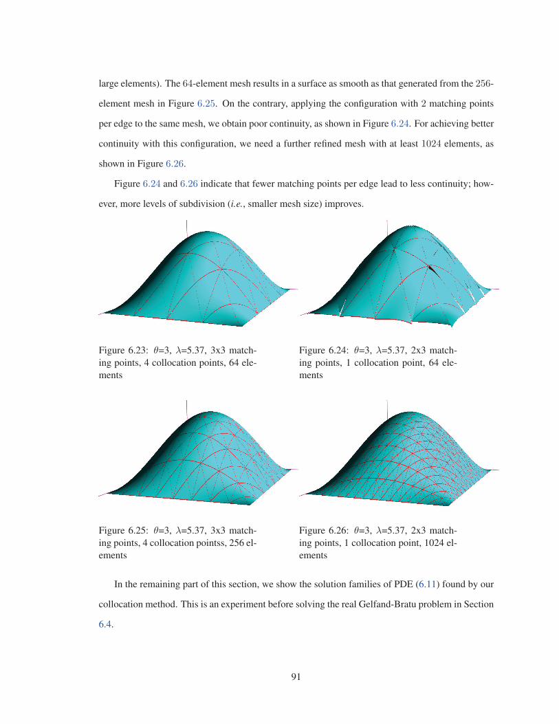
large elements). The 64-element mesh results in a surface as smooth as that generated from the 256-
element mesh in Figure 6.25. On the contrary, applying the configuration with 2 matching points
per edge to the same mesh, we obtain poor continuity, as shown in Figure 6.24. For achieving better
continuity with this configuration, we need a further refined mesh with at least 1024 elements, as
shown in Figure 6.26.
Figure 6.24 and 6.26 indicate that fewer matching points per edge lead to less continuity; how-
ever, more levels of subdivision (i.e., smaller mesh size) improves.
Figure 6.23: θ=3, λ=5.37, 3x3 match-ing points, 4 collocation points, 64 ele-ments
Figure 6.24: θ=3, λ=5.37, 2x3 match-ing points, 1 collocation point, 64 ele-ments
Figure 6.25: θ=3, λ=5.37, 3x3 match-ing points, 4 collocation pointss, 256 el-ements
Figure 6.26: θ=3, λ=5.37, 2x3 match-ing points, 1 collocation point, 1024 el-ements
In the remaining part of this section, we show the solution families of PDE (6.11) found by our
collocation method. This is an experiment before solving the real Gelfand-Bratu problem in Section
6.4.
91

Figure 6.27: Solution families found by our collocation method.Family 1: A stable stationary solution family defined by function (6.10), the numerical solutions ofwhich can also be detected by our collocation method and therefore we can measure the error.Family 2: An unstable stationary solution family defined by function (6.10), which cannot bedetected by our method because it is unstable.Family 3: The stable stationary solution family found by our collocation method; however, itsanalytical form is unknown.
λ θ1 family#1 θ2 family#3
0.1 0.3173 0.00628 19.196 3.7230.5 0.71854 0.03210 14.985 2.401.0 1.03355 0.06605 13.0383 1.872.0 1.51715 0.14057 10.9387 1.403.0 1.93974 0.27036 9.5817 1.184.0 2.35755 0.32904 8.507 1.085.0 2.81155 0.45817 7.548 1.056.0 3.37355 0.64039 6.5766 1.117.0 4.55207 1.08594 5.0545 1.29657.02 4.66823 1.13360 4.932 1.24397.0277 4.8 1.18837 4.8 1.18837
Table 6.21: Solution families found by our collocation method.
92
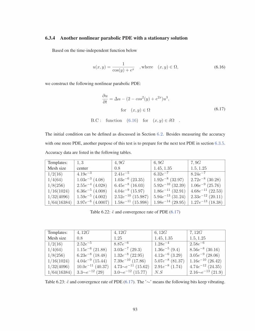
6.3.4 Another nonlinear parabolic PDE with a stationary solution
Based on the time-independent function below
u(x, y) =1
cos(y) + ex,where (x, y) ∈ Ω, (6.16)
we construct the following nonlinear parabolic PDE:
∂u
∂t= Δu− (2− cos2(y) + e2x)u3,
for (x, y) ∈ Ω
B.C : function (6.16) for (x, y) ∈ δΩ .
(6.17)
The initial condition can be defined as discussed in Section 6.2. Besides measuring the accuracy
with one more PDE, another purpose of this test is to prepare for the next test PDE in section 6.3.5.
Accuracy data are listed in the following tables.
Templates: 1, 3 4, 9G 6, 9G 7, 9GMesh size center 0.8 1.45, 1.35 1.5, 1.25
1/2(16) 4.19e−3 2.41e−5 6.32e−7 8.24e−7
1/4(64) 1.03e−3 (4.08) 1.03e−6 (23.35) 1.92e−8 (32.97) 2.72e−8 (30.28)1/8(256) 2.55e−4 (4.028) 6.45e−8 (16.03) 5.92e−10 (32.39) 1.06e−9 (25.76)1/16(1024) 6.36e−5 (4.008) 4.04e−9 (15.97) 1.86e−11 (32.91) 4.68e−11 (22.53)1/32(4096) 1.59e−5 (4.002) 2.52e−10 (15.987) 5.94e−13 (31.24) 2.33e−12 (20.11)1/64(16384) 3.97e−6 (4.0007) 1.58e−11 (15.998) 1.98e−14 (29.95) 1.27e−13 (18.38)
Table 6.22: e and convergence rate of PDE (6.17)
Templates: 4, 12G 4, 12G 6, 12G 7, 12GMesh size 0.8 1.25 1.45, 1.35 1.5, 1.25
1/2(16) 2.52e−5 8.87e−6 1.28e−4 2.58e−6
1/4(64) 1.15e−6 (21.88) 3.03e−7 (29.3) 1.36e−5 (9.4) 8.56e−8 (30.16)1/8(256) 6.23e−8 (18.48) 1.32e−8 (22.95) 4.12e−6 (3.29) 3.05e−9 (28.06)1/16(1024) 4.04e−9 (15.44) 7.39e−10 (17.86) 5.07e−8 (81.37) 1.16e−10 (26.42)1/32(4096) 10.0e−11 (40.37) 4.73∼e−11 (15.62) 2.91e−8 (1.74) 4.74e−12 (24.35)1/64(16384) 3.3∼e−12 (29) 3.0∼e−12 (15.77) N.S 2.16∼e−13 (21.9)
Table 6.23: e and convergence rate of PDE (6.17). The ’∼’ means the following bits keep vibrating.
93

The process of time integration starting from u(x, y, 0) = 0 in the entire domain is visualized
in Figure 6.28 ∼ 6.35:
Figure 6.28: t = 0.01 Figure 6.29: t = 0.02
Figure 6.30: t = 0.03 Figure 6.31: t = 0.04
94
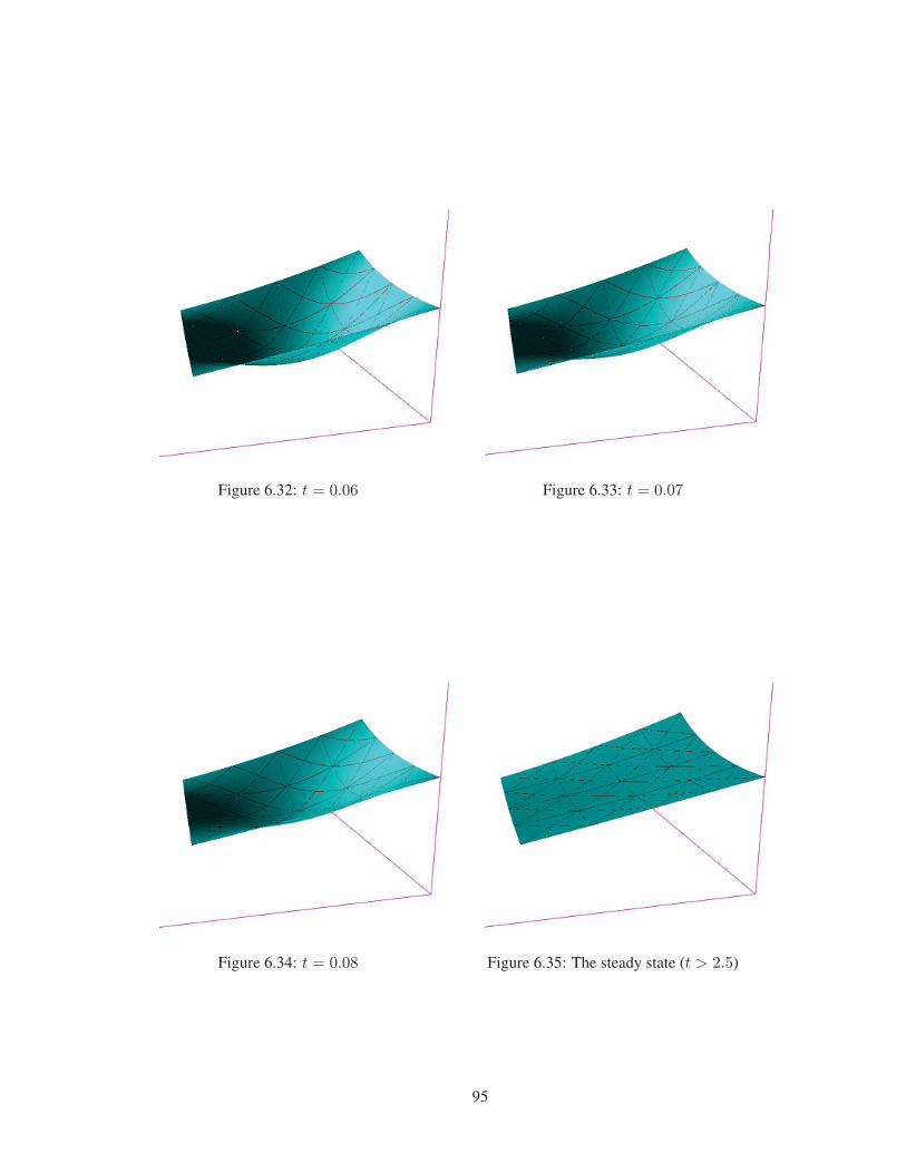
Figure 6.32: t = 0.06 Figure 6.33: t = 0.07
Figure 6.34: t = 0.08 Figure 6.35: The steady state (t > 2.5)
95

6.3.5 A nonlinear parabolic PDE without stationary solution
All parabolic PDEs used in the preceding tests have stationary solutions that can be reached by
time integration. The steady states are the solutions of the corresponding elliptic PDEs, which are
time-independent. Because we know the analytical solutions of the elliptic PDEs, we can measure
the accuracy of the numerical stationary solutions of the PDEs. The accuracy of the steady state
depends on the layout of matching points and collocation points, mesh size, and the collocation
method. In this section we want to see how accuracy is related to the time dimension. For this
purpose, we need to know the analytical solution of the parabolic PDE itself (instead of the corre-
sponding elliptic PDE). Therefore such an analytical solution must be a function of time. Making
reference to the general analytical solution of the Fisher Equation given by Christophe Picard in
[18], we construct a nonlinear parabolic PDE of this type. The analytical solution is defined as
following:
u(x, y, t) =A
cos(By) + e(Cx+Dt),
where (x, y) ∈ Ω
(6.18)
By choosing appropriate values for the coefficients of the above general closed-form solution, we
get the following function:
u(x, y, t) =1
cos(y) + e(x−2t),
where (x, y) ∈ Ω ,
(6.19)
and construct the corresponding nonlinear parabolic PDE:
∂u
∂t= Δu+ u(1− 2u2),
for (x, y) ∈ Ω
B.C : u(x, y, t) =1
cos(y) + e(x−2t)for (x, y) ∈ δΩ
(6.20)
Note that function (6.19) at t = 0 is identical to function (6.16). We first do time integration for
PDE (6.17) until the solution has reached its steady state. Then we take this steady state as the initial
condition from which to start the time evolution for PDE (6.20). We need to reset t = 0. Another
96
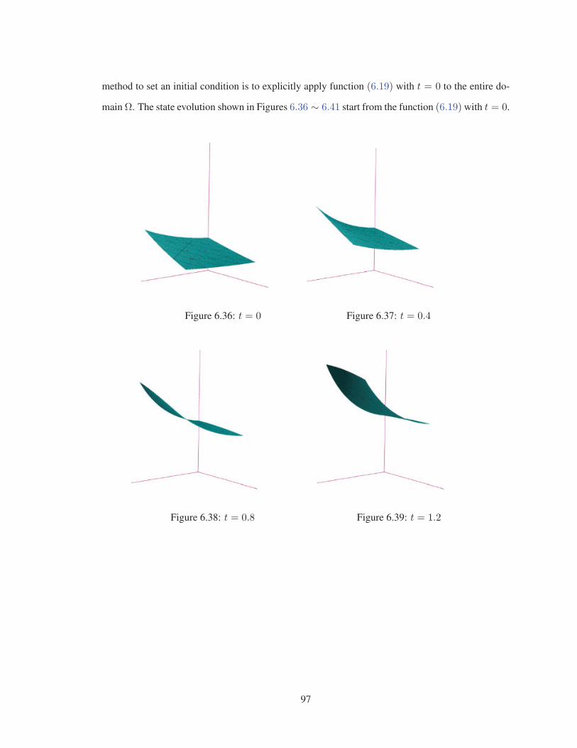
method to set an initial condition is to explicitly apply function (6.19) with t = 0 to the entire do-
main Ω. The state evolution shown in Figures 6.36 ∼ 6.41 start from the function (6.19) with t = 0.
Figure 6.36: t = 0 Figure 6.37: t = 0.4
Figure 6.38: t = 0.8 Figure 6.39: t = 1.2
97
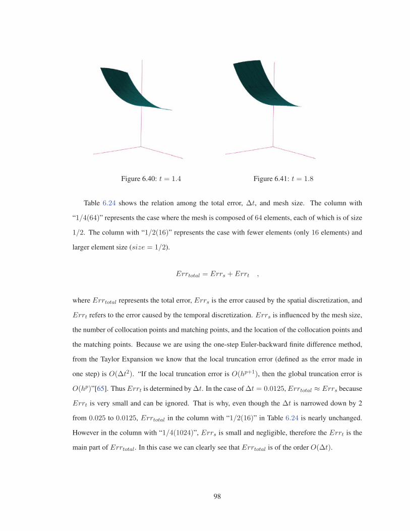
Figure 6.40: t = 1.4 Figure 6.41: t = 1.8
Table 6.24 shows the relation among the total error, Δt, and mesh size. The column with
“1/4(64)” represents the case where the mesh is composed of 64 elements, each of which is of size
1/2. The column with “1/2(16)” represents the case with fewer elements (only 16 elements) and
larger element size (size = 1/2).
Errtotal = Errs + Errt ,
where Errtotal represents the total error, Errs is the error caused by the spatial discretization, and
Errt refers to the error caused by the temporal discretization. Errs is influenced by the mesh size,
the number of collocation points and matching points, and the location of the collocation points and
the matching points. Because we are using the one-step Euler-backward finite difference method,
from the Taylor Expansion we know that the local truncation error (defined as the error made in
one step) is O(Δt2). “If the local truncation error is O(hp+1), then the global truncation error is
O(hp)”[65]. Thus Errt is determined by Δt. In the case of Δt = 0.0125, Errtotal ≈ Errs because
Errt is very small and can be ignored. That is why, even though the Δt is narrowed down by 2
from 0.025 to 0.0125, Errtotal in the column with “1/2(16)” in Table 6.24 is nearly unchanged.
However in the column with “1/4(1024)”, Errs is small and negligible, therefore the Errt is the
main part of Errtotal. In this case we can clearly see that Errtotal is of the order O(Δt).
98

time, mesh size t = 2.0 t = 2.0 t = 2.0Δt 1/16(1024), 4collo 1/4(64), 4collo 1/2(16), 4collo
0.2 5.3339e−4 6.6908e−4 1.1555e−3
0.1 2.5153e−4 (2.12) 3.3625e−4 (1.99) 8.0404e−4 (1.44)0.05 1.2210e−4 (2.06) 1.8720e−4 (1.79) 6.6274e−4(1.21)0.025 6.0163e−5 (2.03) 1.1541e−4 (1.62) 5.9983e−4 (1.11)0.0126 2.9878e−5 (2.01) 8.4404e−5 (1.36) 5.6986e−4 (1.05)
Table 6.24: Dependence of the errors on Δt
6.4 Application
6.4.1 The Gelfand-Bratu problem
The Bratu problem, also called as Liouville–Bratu–Gelfand problem, is an parabolic PDE which
defines a solid fuel ignition model, and is derived as a model for the thermal reaction process in
a combustible, nondeformable material of constant density during the ignition period [63]. This
problem is also often used as a benchmarking tool for numerical methods [62].
∂u
∂t= Δu+ λeu ,
x ∈ Ω ⊂ R2
B.C : u(x, y, t) = 0 for (x, y) ∈ δΩ,
I.C : u(x, y, 0) = 0 for (x, y) ∈ Ω,
(6.21)
where u is the temperature in the problem domain and λ is the parameter. The general Bratu
problem is defined in Rn, but we focus on its 2D case. The heat is generated by the combustion,
diffused in the problem domain, and lost through the boundary of the domain. The temperature is
kept at 0 on the boundary. The combustion is defined by λeu, and the speed of the heat generation
is controlled by parameter λ. For certain values of λ, starting from a specified initial condition and
after a certain period of reaction, the temperature distribution will be stabilized at a stationary state.
With the same values of λ, starting from some other initial condition, the temperature distribution
may approach an equilibrium in a certain period of reaction, but cannot stay at it. Such equilibrium
is an unstable solution of the PDE. For other values of λ, in some or all regions of the domain, the
99

heat is generated always faster than it is transferred away; as the result, the temperature in those
regions keeps increasing until blow-up.
We want to determine the stable stationary solutions of (6.21).
6.4.2 Numerical solution of the Gelfand-Bratu problem in 2D
Starting from λ = 1.0, we do time integration from the initial condition in (6.21). Afterward,
we increase λ by 1 and for each such increased value of λ we start the time integration from the
current stationary solution and, as a result, reach a new stationary solution. This situation continues
until we encounter the critical value of λ at λ ≈ 6.85, where we can no longer reach any steady
state, as shown in Figure 6.42 and Table 6.25.
Figures 6.43 − 6.46 show the stable stationary solutions for cases with λ < 0, which can be
considered as some kind of chemical reaction absorbing heat.
Figure 6.42: The stationary solution families of the Bratu problem. The stationary solution family 1is stable. The stationary solution family 2 is unstable. We can only determine the stable stationarysolution by time integration.
100
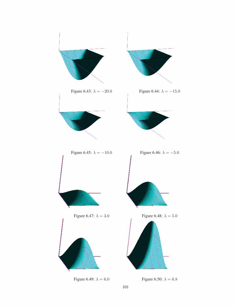
Figure 6.43: λ = −20.0 Figure 6.44: λ = −15.0
Figure 6.45: λ = −10.0 Figure 6.46: λ = −5.0
Figure 6.47: λ = 3.0 Figure 6.48: λ = 5.0
Figure 6.49: λ = 6.0 Figure 6.50: λ = 6.8
101
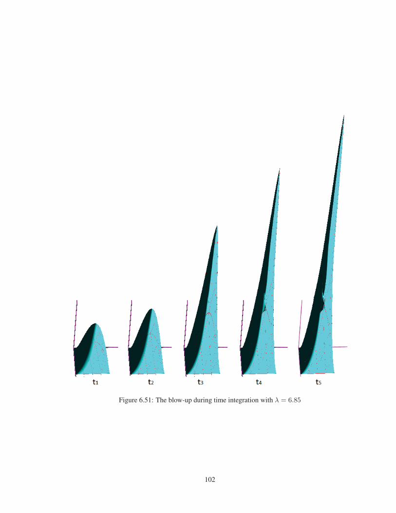
Figure 6.51: The blow-up during time integration with λ = 6.85
102

λ CenterV alue
1.0 0.0772.0 0.1653.0 0.2684.0 0.3935.0 0.5546.0 0.7976.5 1.0146.6 1.0866.7 1.1916.8 1.322
Table 6.25: Bratu solution family found by our collocation method.
Figure 6.52: Test the Bratu problem in another domain, which is smaller than the unit square. Theblow-up takes place when λ = 21.0
103

6.5 Summary of numerical results
In this chapter we have established a scheme, including different configurations of the numbers
and locations of matching points and collocation points, various mesh sizes, etc., to test the accuracy
of numerical solutions found by the piecewise collocation method. Based on the large number of
test results in the preceding section, we have been able to extract some common features about the
relation between accuracy and the schema, as shown in Table 6.26. From the table, we can prac-
tically predict which configurations usually bring more accurate solutions than others, but without
supporting mathematical theory. More research on this topic is needed.
mch−\collo− 1 4 6 7points :\points at center at 0.8 or 1.25 at (1.45, 1.35) at (1.5, 1.25)1G× 3 (22)2G× 33G× 3 2, (24) 1, (25) 1, (24∼5)4G× 3 2 1, (24∼5)
Table 6.26: Accuracy levels and convergence rates of different configurations.
In Table 6.26, ’G’ means the matching points are Gauss points. The values 0.8, 1.25, (1.45, 1.35),
and (1.5, 1.25) indicate collocation point locations, as illustrated by Figure 6.6 in Section 6.1.3. The
colors of cells indicate different performance, including mainly the accuracy, together with conver-
gence rate i.e., the values in () and/or singularity, of the corresponding configurations:
- The white cells represent the preferred configurations with high accuracy and high convergence
rates. The accuracy level 1 is even higher than level 2. Some convergence rates, which are
shown in the parenthesis, are uniform for all mesh sizes. Non-uniform convergence rates are
not shown in the table although some of them are quite high.
- The light gray cells represent workable but un-preferable configurations which bring lower accu-
racy, usually with irregularly varying convergence rates.
- The dark gray cells represent the configurations to be avoided, which cause a non-invertible matrix
(Φ|LΦ), or give divergent results.
104

In all cases, the configurations with the Gauss matching points give higher accuracy than those with
on equally-spaced matching points.
We have also visualized the process of time integration (i.e., state evolution) of the parabolic
PDEs, which is a distinctive feature in comparison to elliptic PDEs. We have shown that, for
finding any stationary solutions of a PDE, different Initial conditions can be chosen and thereby
causing different processes of state evolution, which may (but not necessarily) reach different steady
states (i.e., stationary solutions). Thus, by choosing different initial conditions, it is possible to find
multiple solution families, as shown in test example 6.3.3.
Finally, we applied our method to solving the Bratu problem, where we have found out a family
of stable stationary solutions. We have also located the position of the fold of this family.
105

Chapter 7
Visualization
We have implemented functionality of visualization, which realistically illustrates problem do-
mains, solutions, and any other related info. We have briefly mentioned 2D and 3D visualization in
Section 5.1, when describing the Model-View-Controller architecture. Visualization of data makes
the info “hidden” behind the raw data visible and intuitive for human understanding. Moreover,
visualization makes inter-person communication about the data more effective. However, visualiza-
tion is not for reporting precise values, which should be done by data tables.
The 2D visualization visualizes solutions as height-field, which reflects roughly the shape of
the solution surfaces. Two example solutions are visualized as shown Figure 7.1 and 7.2:
Figure 7.1: 2D visualization of a solu-tion
Figure 7.2: 2D visualization of anothersolution
106

The gray level reflects values within the range of 0.0− 0.1. Once the values exceed this range, the
gray level wraps back; therefore, we can see the “growth rings” or contour bars, which can be used
for imagining the shape of surface and estimating values. We can also get the height value at the
center point of the square domain from a message box, then by counting the number of contour bars
and observing the gray level, we can roughly estimate the value at any specific point. Of course, we
can show the values wherever there is a mouse-click or mouse-over; however, this is not necessary
for this research project. In this chapter we will emphasize the visualization in 3D.
7.1 Pixel-correct mathematical surface rendering
Our visualization guarantees mathematical correctness at each screen space pixel by using the
Ray casting rendering. Pixel-correctness is emphasized in our visualization to make sure the polyno-
mial patches are honestly visualized without any artifact. Figure 7.3 shows the surface of a solution
of the Bratu problem with λ = 4.0 obtained by our discontinuous piece-wise smooth collocation
method. Figure 7.4 shows the same surface after zooming in. It is important to note that, in order
to exaggerate the piecewise, we have chosen a less smooth (or less accurate) configuration for our
collocation method (i.e., 2 matching points per edge, 1 collocation point per element, and less sub-
division, i.e., bigger mesh size) to solve for the solution shown in the figures. Thus, the solution
surface have higher curvature. It is easy to achieve enough smooth and accurate results like those
shown in figure 6.23 and 6.25 with a configuration of more matching or smaller mesh size.
Figure 7.3: A surface over a 64-elementmesh. Each element has 1 collocationpoint and 2 matching points per edge.
Figure 7.4: A zoomed-in view of thesurface for showing the shapes of thepatches and the gaps between each pairof adjacent patches.
107

No matter how largely zoomed in, the surface patches, their silhouettes, and patch edges are always
smooth, as show in the above figures. For our discontinuous piece-wise smooth collocation method,
the visualization must show the conceptual features of the solution surfaces; that is, discontinuity
between two adjacent surface patches, C1 continuity at the matching points, and the local smooth-
ness of patches. If we had used polygon-based rendering, when zooming into the surfaces, we
would have seen polylines (instead of curves) on the silhouettes and edges, and faceted (instead of
smooth) patch surfaces. This kind of artifact or distortion would hide some essential natures of our
collocation method. In general, this problem exists in visualization of many mathematical surfaces
(parametric, explicit, and implicit). Much research has been done for pixel-accurate visualization of
mathematical surfaces; for example, [58], [59], [60], and [61], in which the researchers make use of
geometry shader or tessellation shader of GPUs to dynamically subdivide the original facets. The
researchers of [58] point out that ”no fixed set of levels (of tessellation) can avoid faceted display
or overtessellation”. Thus, tessellation levels should be changed dynamically; in [59], the author
”use the screen space distance between the tessellated surface and the corresponding surface point
as an error metric”, and then adjust tessellation level accordingly to make ”the sampling distance
to meet any given tolerance”. A reasonable threshold of tolerance is that the projection of the dis-
tance to screen space is less than a pixel. This principle is similar to that of our error estimator
for adaptive mesh discussed in Section 2.1. These tessellation-based methods can smooth surfaces;
however, tessellation cannot smooth the edges of patches in our problem, and ”Coarse tessella-
tions near silhouette edges are easily detected” [59], according to the author. Thus, we use the Ray
casting method for rendering, which is absolutely mathematically pixel-correct (not only visually
pixel-accurate), and straightforward to implement. Although this brutal-force method is compu-
tationally expensive, fast technical progress in hardware will compensate the computational cost.
Furthermore, our visualization emphasizes mathematical correctness rather than frame rate (FPS).
Thus, the speed of rendering is not our top consideration as long as the interactivity is acceptable.
108
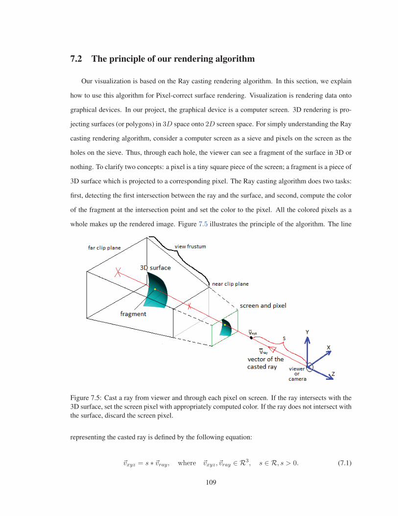
7.2 The principle of our rendering algorithm
Our visualization is based on the Ray casting rendering algorithm. In this section, we explain
how to use this algorithm for Pixel-correct surface rendering. Visualization is rendering data onto
graphical devices. In our project, the graphical device is a computer screen. 3D rendering is pro-
jecting surfaces (or polygons) in 3D space onto 2D screen space. For simply understanding the Ray
casting rendering algorithm, consider a computer screen as a sieve and pixels on the screen as the
holes on the sieve. Thus, through each hole, the viewer can see a fragment of the surface in 3D or
nothing. To clarify two concepts: a pixel is a tiny square piece of the screen; a fragment is a piece of
3D surface which is projected to a corresponding pixel. The Ray casting algorithm does two tasks:
first, detecting the first intersection between the ray and the surface, and second, compute the color
of the fragment at the intersection point and set the color to the pixel. All the colored pixels as a
whole makes up the rendered image. Figure 7.5 illustrates the principle of the algorithm. The line
Figure 7.5: Cast a ray from viewer and through each pixel on screen. If the ray intersects with the3D surface, set the screen pixel with appropriately computed color. If the ray does not intersect withthe surface, discard the screen pixel.
representing the casted ray is defined by the following equation:
�vxyz = s ∗ �vray, where �vxyz, �vray ∈ R3, s ∈ R, s > 0. (7.1)
109

The �vray should be unit vector. We will explain in detail how to compute the �vray. For now, simply
suppose that there is an existing �vray for each pixel on screen so that we can directly make use
of it to probe a fragment. The 3D surface can be any arbitrary mathematical surface. However,
because we are here talking about visualizing the results of our collocation method, we are only
concerned with the surfaces defined in the form of (3.9). Here, we re-write the expression with
some necessary changes to make it conform to the naming convention of the coordinate system in
3D Computer Graphics, which is illustrated in figure 7.5.
y = p(x, z) =n+m∑i=1
ciφi(x, z) ∈ Pn+m. (7.2)
In 3D Graphics, y represents height, which is significantly different from the y in all the preceding
chapters of this thesis.
We need to find the intersection between (7.1) and (7.2); that is, finding a value of s such that point
�vxyz is on the surface.
R(s) = �vxyz.y − p(�vxyz.x, �vxyz.z) = 0, (7.3)
where R(s) is the residual. The unknown s can be solved by using Newton’s method, with the
intersection between the ray and the near clip plane as the initial guess. However, in order to
guarantee Newton iteration converge, the initial guess should be close to the solution. Thus, we
need to find on the ray a point as close as possible to the surface, and then start the Newton iteration
from that point. We use a straightforward method to find such a point; that is, starting from the
near clip plane and tracing the ray, we specify a series of uniformly distributed sampling points.
We denote by s1, s2, . . . , sk these sampling points ordered by their distances away from the viewer.
Then we substitute the values of si into (7.3) to evaluate R(si). If there exist R(sj) and R(sj+1)
having different signs, it indicates that point sj and point sj+1 are located on different sides of
the surface, so the ray must have penetrated the surface and the intersection must be somewhere
between point sj and point sj+1. Thus, sj can be taken as the initial guess of s. If all the values of
R(si) have the same sign, then there are two possibilities: first, the ray does not intersect with the
surface, or second, the ray has penetrated the surface for even times in between certain pair(s) of sj
and sj+1. In the latter case, the interval of probing is not small enough so that the intersection points
110

are skipped and missed. This problem can be solved by redoing the probing from a shifted starting
point, as shown in figure 7.6. Shortening sampling point interval may also be a solution, but it would
increase the number of sampling points and therefore require more computational cost, so it is not
preferable. In figure 7.6(A), all the intersections are missed, but this is not the worst case because at
Figure 7.6: The correct intersection may be missed as illustrated in this figure.The curve represents a surface. The grayed and un-grayed areas represent the two sides of thesurface, respectively. The intersection marked with the red X is expected to be detected as thecorrect intersection because it is the closest one to the viewer S1 . In (A), the sampling points,S1, S2, S3, and S4, with uniform interval L, are all on the same side of the surface and thereforemiss all the intersections; in (B), generate new sampling points S′i by shifting the Si by L/2; asthe result, S′1 and S′2 are still on the same side of the surface, so the expected intersection is stillmissed; however, S′2 and S′3 are on different sides of the surface, so the intersection between S′2 andS′3 can be detected, but it is not the expected. The problem is that, when we have detected such anintersection, we have no idea about whether it is the expected or not.
least the algorithm knows that it must try again with shifted sampling points. The worst case is figure
7.6(B), in which the algorithm has missed the correct intersection but instead detected a wrong one
(between S′2 and S′3) and took it as the correct intersection. Additionally, correct intersections might
also be missed in some other possible cases with complicated surfaces. Fortunately in practice, the
prerequisite of using this method to determine the initial guess is that the surface patch over each
element has already been sufficiently ”flattened” by adaptive mesh generation. In consequence, the
case in 7.6(B) is very rare. In this algorithm, we stop probing once hitting the first intersection.
(For rendering semi-transparent surfaces, we would have to detect all intersections along the ray
and compute weighted average color of them.)
Up to this point, we have explained the essential principle of our ray casting rendering method.
It seems to be perfect except for one problem; that is, time consuming because we have to do the
above computation one-by-one for all the pixels on screen. In fact this is not true because the
111

rendering and the related computation of all the pixels will be done in parallel at the same time by
GPU, which will be discussed in next section.
7.3 Technical details
We will begin this section with briefly explaining OpenGL’s rendering pipeline because it is the
base on top of which our visualization method has been designed and implemented. Then we will
explain how our ray casting algorithm is involved into the rendering pipeline. Our algorithms and
methods are generally feasible on any graphics libraries which supports directly GPU programming,
including OpenGL/GLSL, WebGL, and DirectX/HLSL, with C++, Java, C#, or JavaScript.
A visualization application is conceptually composed of two sides: the CPU side and GPU
side. On the CPU side, we construct the 3D objects to render. A 3D object is a group of triangular
facets. The geometric data (vertices, normal vectors, vertex indices, etc.) of each facet is generated
on the CPU side by computing it on-the-fly or loading it from 3D model files. Then the data
is transferred to the GPU side and stored into the appropriate buffers through OpenGL functions
(or DirectX functions, depending on which 3D library we are using). Then OpenGL begins to
process the data. OpenGL implements what’s commonly called a rendering pipeline, which is a
sequence of processing stages for converting the data your application provides to OpenGL into a
final rendered image [64]. OpenGL then processes the data through a sequence of shader stages:
vertex shading, tessellation shading (which itself uses two shaders), and finally geometry shading,
before it’s passed to the rasterizer. The rasterizer will generate fragments for any primitive that’s
inside of the clipping region, and execute a fragment shader for each of the generated fragments
[64]. Tessellation and geometry shading are two optional stages, which are not involved in our
rendering algorithm; our algorithm replies on only two stages: vertex shading and fragment shading
(also called pixel shading). We use an example to explain how our algorithm is implemented in
the vertex shader and fragment shader in OpenGL’s rendering pipeline. In the example, we will
render a single mathematical surface, y = f(x, z), where (x, z) ∈ [0, 1]. For simplicity, we assume
the range of f(x, z) is also [0, 1]. Thus, in the application on the CPU side, we construct a unit
cube, which means 8 vertices, 2 × 6 triangle facets, and the corresponding vertex indices. Also
112

on the CPU side, we prepare matrices which defines the transformation (i.e., translation, rotation,
and scaling) of the cube. Then we start OpenGL’s rendering pipeline to render this set of geometry
data. First, vertex shading, which is a programmable stage. For our visualization, we write a simple
vertex shader which does nothing more than computing the vertex transformation and declaring a
few in-GPU variables which will be accessed from within fragment shader. The vertex shader can
see only each individual vertex. It does not have any knowledge about facets (or primitives, in
the term of OpenGL). Facets are constructed at next stage: Primitive Assembly, which organizes
the vertices into their associated geometric primitives in preparation for clipping and rasterization
[64]. After rasterization, a facet will be decomposed into a group of fragments, each of which
will be computed and assigned appropriate color at the stage of fragment shading (also called pixel
shading). Fragment shading is also a programmable stage, and the program is called fragment
shader. Instead of computing the color and light for the fragments composing the planar facets
of the cube, our fragment shader computes the color and light for the corresponding fragments on
the mathematical surface, y = f(x, z), the 3D location of which is determined by using our ray
casting algorithm explained in Section 7.2. in Section 7.2, we have omitted the explanation of how
to compute the ray vector �vray to this section. Now, it can be easily explained. We can get the 3D
location of each individual fragment via the in-GPU variable declared and set in the vertex shading
stage. Thus, �vray can be calculated the following way:
�vray = normalize(�vfrag − �vviewer), (7.4)
where �vfrag is the location of fragment and �vviewer is the location of viewer. �vray is normalized and
therefore unit vector.
After determining the 3D location of a fragment on the mathematical surface, we can compute the
normal vector at that point on the surface, and thereby compute the light at that point. The result of
this example is shown in figure 7.7 and 7.8.
The main idea of our ray casting method is, first, constructing a container object (in this exam-
ple, the unit cube), then make OpenGL’s rendering pipeline draw the container object, and thereby
113
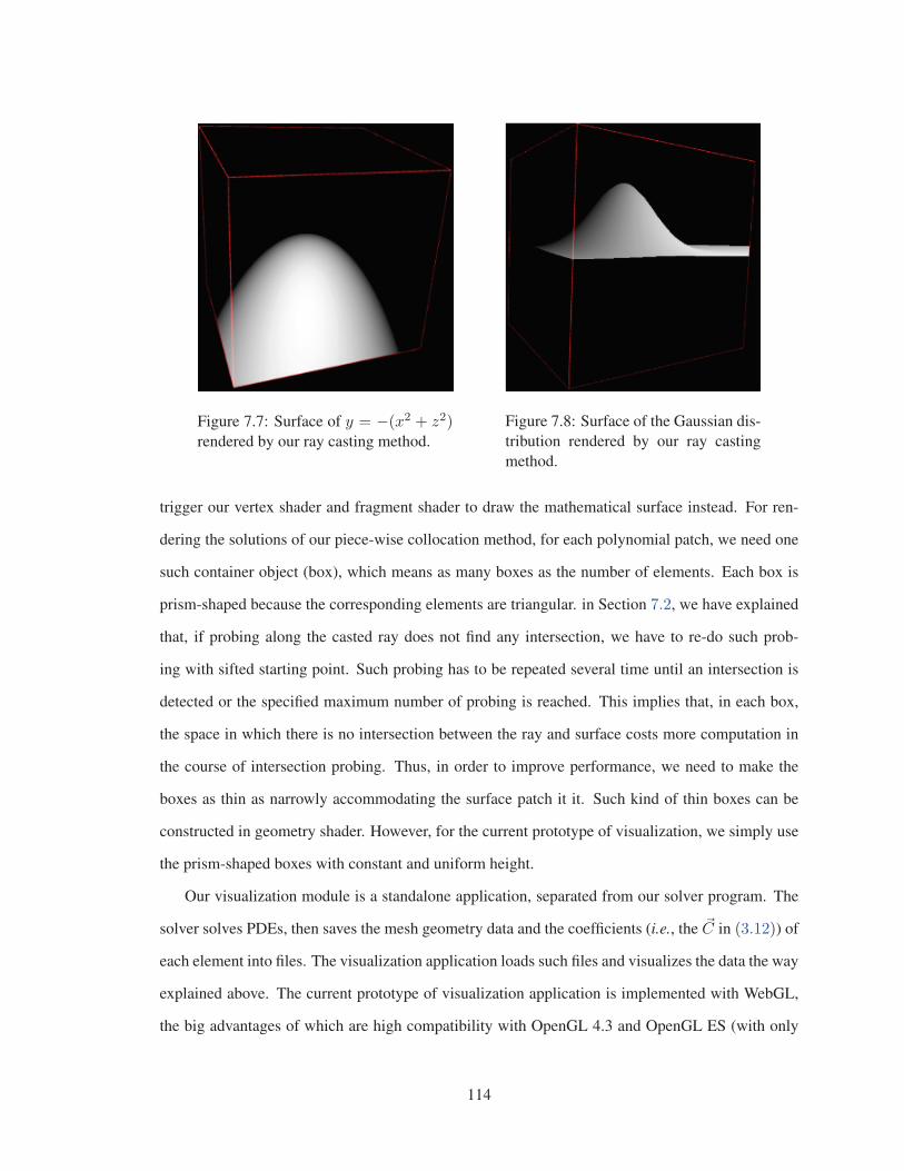
Figure 7.7: Surface of y = −(x2 + z2)rendered by our ray casting method.
Figure 7.8: Surface of the Gaussian dis-tribution rendered by our ray castingmethod.
trigger our vertex shader and fragment shader to draw the mathematical surface instead. For ren-
dering the solutions of our piece-wise collocation method, for each polynomial patch, we need one
such container object (box), which means as many boxes as the number of elements. Each box is
prism-shaped because the corresponding elements are triangular. in Section 7.2, we have explained
that, if probing along the casted ray does not find any intersection, we have to re-do such prob-
ing with sifted starting point. Such probing has to be repeated several time until an intersection is
detected or the specified maximum number of probing is reached. This implies that, in each box,
the space in which there is no intersection between the ray and surface costs more computation in
the course of intersection probing. Thus, in order to improve performance, we need to make the
boxes as thin as narrowly accommodating the surface patch it it. Such kind of thin boxes can be
constructed in geometry shader. However, for the current prototype of visualization, we simply use
the prism-shaped boxes with constant and uniform height.
Our visualization module is a standalone application, separated from our solver program. The
solver solves PDEs, then saves the mesh geometry data and the coefficients (i.e., the �C in (3.12)) of
each element into files. The visualization application loads such files and visualizes the data the way
explained above. The current prototype of visualization application is implemented with WebGL,
the big advantages of which are high compatibility with OpenGL 4.3 and OpenGL ES (with only
114

some minor differences) and platform-independent. It can run on all web browsers (IE11, FireFox,
etc.) on all OSs (Window, Mac/OS, Linux, ...).
Also because our visualization prototype is a standalone application and web-based, it is easy
to be further developed as a formal on-line mathematical surface visualization tool. Any users can
make use of this on-line tool to visualize their numerical solutions as long as they follow our data
file structure and use the same set of basis.
115
Chapter 8
Conclusions and Discussion
In this thesis we have presented the implementation of a novel collocation method for solving
nonlinear parabolic partial differential equations (PDEs). The temporal partial derivative is dis-
cretized using the implicit Euler backward finite difference scheme. The 2D spatial domain of the
PDEs is discretized with triangular adaptive meshes. We have designed and implemented our algo-
rithm of error estimate and the mesh refinement based on it. The refinement method is based on the
Rivara algorithm. For simplicity, our current mesh refinement works separately from time integra-
tion, i.e., mesh refinement is not executed in the course of time integration. Furthermore, we can
generate meshes for irregular polygonal domains. The goal of triangular mesh refinement, support-
ing domains of complex shapes, and solving nonlinear PDEs has been achieved by our collocation
method prototype.
We have used a large number of test cases to measure the accuracy of our collocation method in
Chapter 6. The test results have shown high accuracy. The accuracy of collocation methods depends
on mesh size, mesh shape, the number of collocation points, the location of collocation points, the
number of matching points, and the location of matching points. There is no completely established
mathematical theory for error estimate based on these factors. Some researchers have mathemat-
ically proved the error estimates for some special cases, but not for general cases. However from
the results of our tests we have extracted patterns (i.e., the layouts of various number of collocation
points and matching points) which bring high accuracy and good performance of convergence prop-
erties, as summarized in Section 6.5 and Table 6.26. We have also found some bad patterns which
116

lead to singularity or non-convergence. We have analyzed the singularity caused by some patterns
at the end of Section 3.3. Furthermore, we have used our collocation method solver to find a family
of stable stationary solutions of the Bratu problem.
We have also designed and implemented our own visualization algorithm to display the nu-
merical solutions. Our visualization algorithm is pixel-correct, which means that each pixel of the
rendered 2D image of the mathematical surface in 3D space accurately reflects the position, cur-
vature, and orientation of the corresponding fragment on the surface. For the pixel-correctness, we
directly render the original surfaces instead of polygonal facets generated to approximate the math-
ematical surfaces. We have made use of GPU programming techniques and WebGL to implement
this algorithm. Our visualization program is Web-based and therefore fully platform independent.
It can be further developed as a more general on-line visualization tool.
From the view point of software engineering, it would be interesting optimize our current solver.
In this prototype, we have implemented multi-threading for taking advantage of the parallelism
of the nested dissection algorithm and multi-core CPUs. The acceleration brought by the multi-
threading is obvious in our tests. Integrating the mesh refinement with the time evolution would
bring excellent effect of mesh-moving when solving time-dependent PDEs. For these improve-
ments, the data structure will still be based on linked list because it supports effectively adding or
removing nodes. On the other hand, linked list costs more time for accessing individual nodes and it
breaks locality of reference, which is critically important for CPU cache. Thus, customized memory
management system will be needed for solving these problems.
117

Bibliography
[1] P.J. Olver. “Applied Mathematics Lecture Notes” Available at www.math.umn.edu in directory
/ olver/am /npd.pdf, University of Minnesota, Chapter 22, 2014.
[2] M.M. Kajotoni. “A Comparative Study of Collocation Methods for the Numerical Solution of
Differential Equations” thesis for the degree of Master of Science, School of Mathematical
Sciences, University of KwaZulu-Natal, Durban, pp.1, 2008.
[3] “Partial differential equation” Available at https://en.wikipedia.org in directory
/wiki/Partial differential equation, Wikipedia, 2015.
[4] J. Wang. “Why don’t differential equations of physics go beyond the second order?”
Available at https://www.quora.com/Why-dont-differential-equations-of-physics-go-beyond-
the-second-order, www.quora.com, 2015.
[5] S. Casas, Akhmeteli and NikolajK. “Why are differential equations for fields in physics
of order two?” Available at http://physics.stackexchange.com/questions/18588/why-are-
differential-equations-for-fields-in-physics-of-order-two, physics.stackexchange.com, 2011.
[6] “Ostrogradsky instability” Available at https://en.wikipedia.org/, in directory
wiki/Ostrogradsky instability, Wikipedia, July 2016.
[7] B. Zheng. “Finite Element Approximations of High Order Partial Differential Equations”
Available from https://etda.libraries.psu.edu/catalog/8776, The Graduate School Department
of Mathematics, Pennsylvania State University, 2008.
118

[8] A.P.S. Selvadurai. “Partial Differential Equations in Mechanics 1”, Springer, Section 4.4,
pp.140-142, 2008.
[9] A. Jeffrey. “Applied Partial Differential Equations: An Introduction”, Academic Press, Uni-
versity of Newcastle-upon-Tyne, Section 3.2, pp.118-119, 2003.
[10] C.T. Kelley. “Solving Nonlinear Equations with Newton’s Method”, SIAM Section 1.9.2,
pp.18-19, 2003.
[11] F.Chinesta, R. Keunings and A. Leygue. “The Proper Generalized Decomposition for Ad-
vanced Numerical Simulations: A Primer” Springer, pp.viii, 2014.
[12] T.V. Petersdorff and C. Schwab. “Numerical Solution of Parabolic Equation in High Dimen-
sions” University of Maryland and ETH Zurich, 2002.
[13] A. Falco. “Algorithms and Numerical Methods for High Dimensional Financial Market Mod-
els” Universidad CEU Cardenal Herrera, Valencia, Spain, 2010.
[14] P. Tremblay. “2-D, 3-D and 4-D Anisotropic Mesh Adaptation for the Time-Continuous Space-
Time Finite Element Method with Applications to the Incompressible Navier-Stokes Equa-
tions” Department of Mechanical Engineering, University of Ottawa, 2007.
[15] J.-D. Bopissonnat and M. Yvinec. “Mesh Generation in Higher Dimensions” INRIA Geomet-
rica team, Sophia Antipolis, France.
[16] A.D. Polyanin and A.V. Manzhirov. “Handbook of Math for Engineers and Scientists” Chap-
man & Hall/CRC, 2007.
[17] H. Sharifi. “Collocation Methods for The Numerical Bifurcation Analysis of Systems of Non-
linear Partial Differential Equations” Department of Computer Science, Concordia University,
pp.34,37,39,43,81,169, 2005.
[18] C. Picard. “A Posteriori Error Estimator Framework for PDE’s” Available from
https://www.math.u-bordeaux.fr/ picard/publications/thesis.pdf, Faculty of the Department of
Computer Science, University of Houston, 2007.
119

[19] “Backward Euler method” Available at https://en.wikipedia.org in directory
/wiki/Backward Euler method, Wikipedia.
[20] Q. Zheng. “Collocation Methods for Linear Parabolic Partial Differential Equations”, Depart-
ment of Computer Science, Concordia University, pp.12,16,26,54, 2005.
[21] W. Sun, L. Wu and X. Zhang1. “Nonconforming Spline Collocation Methods in Irregular Do-
mains” Department of Mathematics, City University of Hong Kong and Laboratory of Com-
putational Physics, Institute of Applied Physics and Computational Mathematics, 2007.
[22] Y. He and W. Sun2. “Nonconforming Spline Collocation Methods in Irregular Domains II: Er-
ror Analysis” Faculty of Science, Xi’an Jiaotong University and Department of Mathematics,
City University of Hong Kong, 2007.
[23] S.A. Odejide and Y.A.S. Aregbesola. “A Note on Two Dimensional Bratu Problem” Depart-
ment of Mathematics, Obafemi Awolowo University, Ile-Ife, Nigeria, March 28 2006.
[24] Jonathan Richard Shewchuk. “Theoretically Guaranteed Delaunay Mesh Generation”, UC
Berkeley, Short Course Fourteenth International Meshing Roundtable, San Diego, 11 Septem-
ber 2005.
[25] J.R. Shewchuk. “Delaunay Refinement Mesh Generation” School of Computer Science, Com-
puter Science Department, Carnegie Mellon University, Pittsburgh, PA Submitted in partial
fulfillment of the requirements for the degree of Doctor of Philosophy, May 18, 1997.
[26] L. Komzsik. “Applied Calculus of Variations for Engineers (Second Edition)’,’ CRC Press,
TABLE-12.2, pp.199, 2009.
[27] E. Doedel and H. Shari. “Collocation Methods for Continuation Problem in Nonlinear Elliptic
PDEs” Department of Computer Science, Concordia University, Montreal, Canada, 2005.
[28] E. Doedel. “Collocation Methods for Continuation Problem in Nonlin-
ear Elliptic PDEs” at Journal of Difference Equations and Applications on
https://www.researchgate.net/publication, Concordia University, Montreal, Canada, June
1997.
120
[29] M.S. Gockenbach. “Lecture note of NUMERICAL OPTIMIZATION, The spec-
tral theorem for symmetric matrices” Available at http://www.math.mtu.edu/ ms-
gocken/ma5630spring2003/lectures/spectral/spectral/node2.html, Department of Mathe-
matical Sciences, Michigan Tech, 2003.
[30] “Gaussian filter” Available at en.wikipedia.org in directory /wiki/Gaussian filter, Wikipedia,
2016.
[31] J.R. Sack and J. Urrutia. “Handbook of Computational Geometry - 1st Edition” North Holland,
pp.299, 1999.
[32] M. Bern and P. Plassmann. “Mesh Generation” Available at http://www.ics.uci.edu in direc-
tory / eppstein/280g/Bern-Plassman-meshgen.pdf, Handbook of Computational Geometry, El-
sevier Science, pp.291-332, pp.4, 2000.
[33] D.C. Arney and J.E. Flaherty. “An Adaptive Mesh-Moving and Local Refine-
ment Method for Time-Dependent Partial Differential Equations” Available at
http://www.dtic.mil/dtic/tr/fulltext/u2/a268425.pdf, United States Military and Rensse-
laer Polytechnic Institute, pp.3-4, 1990.
[34] T. Gratsch and K.-J. Bathe. “A posteriori error estimation techniques in practical finite element
analysis” Computers & Structures, Vol 83, Issues 4–5, pp.235–265, January 2005.
[35] S. Prudhomme, J.T. Oden, T. Westermann, J. Bass and M.E. Botkin. “Practical methods for
a posteriori error estimation in engineering applications” Numerical Methods in Engineering,
Vol 56, Issue 8, pp.1193–1224, February 2003.
[36] S. Repin. “A Posteriori Error Estimation Methods for PDE’s” Saint Petersburg Institute of
Mathematics and University of Jyvaskyla, pp.5,26, Zurich Summer School, 2012.
[37] K.I. Joy, “On-Line Geometric Modeling Notes - Bernstein Polynomials” Visualization and
Graphics Research Group, Department of Computer Science, University of California, Davis,
pp.8, 2000.
121

[38] Wikipedia. “Pivot element”, Available at en.wikipedia.org in directory
/wiki/Pivot element#Scaled pivoting, Wikipedia, 2016.
[39] “Neumann boundary condition”, Available at en.wikipedia.org in directory
/wiki/Neumann boundary condition, Wikipedia, 2017.
[40] A. Selman, A. Merrouche and C. Knopf-Lenoir. “3D Mesh Refinement Procedure Using The
Bisection And Rivara Algorithms With Mesh Quality Assessment” Netherlands Institute for
Metals Research and Universite de Technologie de Compiegne, 2001.
[41] “Dirichlet boundary condition”, Available at en.wikipedia.org in directory
/wiki/Dirichlet boundary condition, Wikipedia, 2017.
[42] M.-C. Rivara, A. Merrouche and C. Knopf-Lenoir. “Review on Longest Edge Nested Algo-
rithms” Springer, 2010.
[43] D.N. Arnold and A. Mukherjeey. “Tetrahedral Bisection And Adaptive Finite Elements”
Springer, 1999.
[44] B. Murgante, O. Gervasi, S. Misra, N. Nedjah, A.M.A.C. Rocha, D. Taniar and B.O. Apduhan.
“Computational Science and Its Applications” ICCSA 2012, Part 1, pp.201, Springer, 2012.
[45] M.-C. Rivara and P. Inostroza, edited by Ricardo and Baeza-Yatesn. “A COMPARISON of
Algorithms for the Triangulation Refinement Problem” Computer Science 2: Research and
Applications, Springer, pp.47, Springer, 1993.
[46] C. Bedregal and M.-C. Rivara. “A Study on Size-Optimal Longest Edge Refinement Algo-
rithms” Proceedings of the 21st International Meshing Roundtable, Springer, pp.121-136,
2013.
[47] J.M. Gonzalez-Yuste, R. Montenegro, J.M. Escobar, G. Montero and E. Rodrıguez. “Imple-
mentation of a Refinement/Derefinement Algorithm for Tetrahedral Meshes” University In-
stitute of Intelligent Systems and Numerical Applications in Engineering, University of Las
Palmas de Gran Canaria, 2004.
122

[48] “Fisher’s equation” Available at en.wikipedia.org in directory wiki/Fisher’s equation,
Wikipedia, 2016.
[49] A. Plaza, M.A. Padron and G.F. Carey. “A 3D refinement/derefinement algorithm for solving
evolution problems” Department of Mathematics, University of Las Palmas de Gran Canaria,
Spain, pp.2,16,17, 2000.
[50] M. Trott. “Delta Function” Available at mathworld.wolfram.com/DeltaFunction.html, Wol-
fram Mathworld, 2006.
[51] U. Ascher, J. Christiansen and R. D. Russell. “A Collocation Solver for Mixed Order Systems
of Boundary Value Problems” American Mathematical Society, Mathematics of Computation,
Vol. 33, No. 146, pp.659-679, 1979.
[52] Yu.A. Kuznetsov. “Elements of Applied Bifurcation Theory, Second Edition” Springer, Ap-
plied mathematical sciences, vol. 112, 1998.
[53] A. Dhooge, W. Govaerts, Yu.A. Kuznetsov, W. Mestrom, A.M. Riet and B. Sautois. “MAT-
CONT and CL MATCONT: Continuation toolboxes in matlab” University Gent, Belgium and
Utrecht University, Netherlands, August 2011.
[54] A. Dhooge, W. Govaerts, Yu.A. Kuznetsov and B. Sautois. “Matcont : A Matlab package
for dynamical systems with applications to neural activity” Journal ACM Transactions on
Mathematical Software (TOMS), Vol. 29, Issue 2, pp.141-164, June 2003.
[55] A. Dhooge, W. Govaerts, Yu.A. Kuznetsov, W. Mestrom, A.M. Riet and B. Sautois. “DDE-
BIFTOOL Manual - Bifurcation analysis of delay differential equations” Cornell University,
Jun 2014.
[56] E. Doedel, A. Champneys, F. Dercole, T. Fairgrieve, Yu. Kuznetsov, B. Oldeman, R. Paffen-
roth, B. Sandstede, X. Wang and C. Zhang. “Auto Software for Continuation And Bifurcation
Problems in Ordinary Differential Equations” Available at http://indy.cs.concordia.ca/auto/,
Concordia University, 1996.
123

[57] B. Jacob and G. Guennebaud, written and maintained by volunteers. “Eigen is a C++ tem-
plate library for linear algebra: matrices, vectors, numerical solvers, and related algorithms”,
eigen.tuxfamily.org, 2010
[58] Y.I. Yeo, L. Bin and J. Peters. “Efficient Pixel-Accurate Rendering of Curved Surfaces” Uni-
versity of Florida and Advanced Micro Devices, 2012.
[59] J. Hjelmervik. “Direct Pixel-Accurate Rendering of Smooth Surfaces” Springer, International
Conference on Mathematical Methods for Curves and Surfaces, pp.238-247, 2012.
[60] Y.I. Yeo, S. Bhandare and J. Peters. “Efficient Pixel-accurate Rendering of Animated Curved
Surfaces” Springer, International Conference on Mathematical Methods for Curves and Sur-
faces, pp.491-509, 2012.
[61] C. Figueroa and Raquel. “Real time rendering of parametric surfaces on the GPU” Universi-
dade da Coruna, Spain, 2013.
[62] R. Buckmir. “On exact and numerical solutions of the one-dimensional planar Bratu problem”
Mathematics Department, Occidental College, Los Angeles, U.S.A. 2003.
[63] J. Jacobsen and K. Schmitt. “The Liouville Bratu Gelfand Problemfor Radial Operators” De-
partment of Mathematics, Pennsylvania State University and University of Utah. 2001.
[64] D. Shreiner, G. Sellers, J. Kessenich and B. Licea-Kane. “OpenGL Programming Guide:
The Official Guide to Learning OpenGL, Version 4.3” The Khronos OpenGL ARB Working
Group. 2013.
[65] H. Wang. “AMS 147 Computational Methods and Applications, Lecture 09” Available at
users.soe.ucsc.edu/ hongwang/AMS147/Notes/Lecture09.pdf, UCSC
124
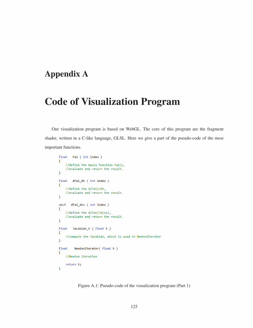
Appendix A
Code of Visualization Program
Our visualization program is based on WebGL. The core of this program are the fragment
shader, written in a C-like language, GLSL. Here we give a part of the pseudo-code of the most
important functions.
Figure A.1: Pseudo-code of the visualization program (Part 1)
125
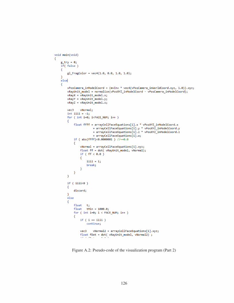
Figure A.2: Pseudo-code of the visualization program (Part 2)
126

Figure A.3: Pseudo-code of the visualization program (Part 3)
127