Collision Detection with Relative Screw Motion

Samuel R. Buss∗

Department of MathematicsUniv. of California, San Diego

La Jolla, CA 92093-0112

October 11, 2004

Keywords: Collision detection, screw motion, rigid body collision, propercollision, rasterization.

AbstractWe introduce a framework for collision detection between a pair of

rigid polyhedra. Given the initial and final positions and orientationsof two objects, the algorithm determines whether they collide, and if so,when and where. All collisions, including collisions at different times,are computed at once along with “properness” values that measurethe extent to which the collisions are between parts of the objects thatproperly face each other. This is useful for handling multiple (nearly)concurrent collisions and contact points.

The relative motions of the rigid bodies are limited to screw mo-tions. This limitation is not always completely accurate, but we canestimate the error introduced by the assumption.

Our implementation uses rasterization to approximate the positionand time of the collisions. This allows level-of-detail techniques thatprovide a tradeoff between accuracy and computational expense.

The collision detection algorithms are only approximate, both be-cause of the screw motion assumption and because of the rasterization.However, they can be made robust so as to give consistent informationabout collisions and to avoid sensitivity to roundoff errors.

1 Introduction

Collision detection is important for physical simulations and motion plan-ning. It is also a difficult problem, especially since collision detection must

∗Supported in part by NSF grants DMS-0100589 and DMS-0400848. Email:sbuss@ucsd.edu

1

be fast, robust, and tolerant of roundoff errors. This paper presents analgorithm for collision detection between two moving, polygonally modeledobjects. Our original motivations were detecting collisions in computer game(in particular racing games) where collision detection must be performed onobjects moving at high speed. In this situation, objects frequently are foundto be significantly interpenetrating and may even completely pass througheach other in a single simulation step. Thus the algorithm is designed tocorrectly detection collisions in these situations. In addition, the algorithmdiscovers multiple collisions, not just the first collisions. This allows han-dling multiple collisions at high speeds and maintaining multiple contactpoints between statically contacting objects.

The algorithm takes as input the initial position1 and a final position foreach object, and estimates the intermediate relative motions of the objects asa screw motion. The algorithm computes whether a collision occurs duringthe motion from the initial position to the final position. A single pass ofthe algorithm determines the times and positions of the collisions: there isno need to “back up” time or do a binary search to find the time where theobjects first interpenetrate.

The algorithm computes simultaneously all the collisions between theinitial and final positions, not just the first collision(s). Collisions are clas-sified as to how “proper” they are, where the proper-ness depends on howwell the objects are facing each other locally at the collision. This datacan be used by subsequent application-dependent algorithms to recognizeconcurrent collisions.

For detecting collisions at intermediate times, the objects’ relative mo-tion is assumed to be screw motion. A screw motion consists of rigid bodyrotation around a fixed axis combined with a translation parallel to the axis.This assumption of screw motion is not always exactly correct, but is no lessreasonable than other common assumptions, such as rotation combined witharbitrary translation. In addition, the error introduced by assuming screwmotion can be quantified as being quite small (see Section 4.3).

Several other authors have used screw motion for collision detection:Rossignac and J. Kim [49] advocate the use of screw motions for intermediaterelative motion, and Kim-Rossignac [25] and Redon et al. [45] use screwmotions for collision detection.

The principal idea behind our algorithm is that the relative screw motioncauses the two objects to move towards each along a fixed track, with norotation beyond the curvature induced by the curvature of the “track.” This

1By “position,” we mean both position and orientation.

2

allows us to set up a curved “collision screen,” and project the two objectsonto the collision screen (similar in spirit to the way that objects can beorthogonally projected onto a flat plane). Lines and edges are drawn ontothe collision screen, and collisions are found by examining where the twoobjects project to common points on the screen.

A second idea behind our algorithm is that every collision is given aproperness rating: Since the algorithm reports multiple collisions during atime step it is useful to find the true “first collisions.” The properness valueshelp identify true collisions. A nonnegative properness value indicates thefacets are correctly facing each other at the instant of collision, as wouldoccur for a true first collision. Negative values of properness indicate thefacets are not correctly facing each other and that it is not a first collision.Negative properness values close to zero indicate collisions that are close toproper, and we have found it useful to use slightly improper collisions astrue collisions for handling high-speed collisions. Sections 3 and 5 discussproperness in more detail.

The implemented version of our algorithm uses solid, rigid objects de-fined by polygonal surfaces. It allows arbitrary such objects, including non-convex objects. The implemented form of the algorithm works well withobjects that are not too far from convex, but it could be extended to handlehighly nonconvex objects (e.g., a screw in a screw hole).

The algorithm can readily be adapted to work with non-closed objectsor with objects that are not manifolds. As long as the local adjacencyinformation for polygons is known, it is possible to calculate properness ofcollisions, even for non-manifolds.

We describe an implementation of the collision algorithm that uses ras-terization rather than the analytic methods used by Kim-Rossignac [25] andRedon et al. [45]. Our algorithm differs from those in that it looks for col-lisions between the entire two polyhedra at once, rather than treating thefacets of the polyhedra individually. This allows our algorithm to be robustand tolerant of roundoff errors. Furthermore, adjusting the resolution of therasterization allows a tradeoff of accuracy against computational cost.

Our collision detection algorithm is intended as only one component ofa large scale simulation of collisions and contacts between multiple movingbodies. Once there are very many moving objects, it is too time-consumingto check for collisions between all pairs of objects. Instead, space partitioningalgorithms (e.g., octrees, BSP trees, k-d trees) can be used to prune theset of possible collisions, and bounding volumes (swept spheres, OBBs, k-DOPs, etc.) can be used to quickly decide that many objects to do notcollide (c.f., [14, 24, 21, 31, 47, 44, 57]). It is intended that our algorithm

3

would be used after these preliminary tests to check all remaining potentiallycolliding pairs of objects. Subsequently, the data from our collision detectionalgorithm would be used by application-dependent algorithms to decide howto handle the collisions, e.g., to calculate the forces, or changes in motion,that result from the collisions. It is beyond the scope of this paper toconsider space partitioning and hierarchical methods, or how to calculatecollision responses. Rather, we only examine the question of determiningwhether and how a single pair of rigid objects has collided.

2 Prior Work and Motivations

Early papers on collision detection include [6, 7, 10], and the field has sincegrown too large for us to survey here. (See [37] for a survey.) Instead, wediscuss only some of the more relevant work in order to contrast it with ouralgorithm — our primary focus is the collision of rigid polyhedral objects.

A number of collision detection algorithms work with convex objects.These include algorithms by Lin and Canny [35, 36] exploiting the Voronoidiagram of the space around convex objects and the linear algebra basedmethods of Gilbert et al. [19], as well as many enhancements of these al-gorithms (cf. [9, 39]). These algorithms compute the distance between twonon-overlapping convex bodies; if the convex bodies are interpenetrating,this is detected, but the algorithms do not reliably decide how they collided.Instead, when two moving bodies are discovered to be interpenetrated, thentime is “backed up” and a binary search procedure (bisection) is used to findthe approximate time and position of the first collision between the convexbodies. These algorithms may, however, miss collisions where the bodiespass through each other in a single simulation step.

Another class of algorithms attempts to deal directly with interpene-trating objects, particularly convex objects. [12, 1, 26] give algorithms forfinding the minimum interpenetration distance of two overlapping convexbodies. [27] extend these algorithms to apply to nonconvex objects usingdecomposition into convex pieces. All these algorithms, like our own, at-tempt to deal directly with bodies that may be interpenetrating and canbe used to estimate the collision times and positions. Unlike our algorithm,they restrict to purely translational motion.

Various techniques are used to speed up the collision detection algo-rithms. First, coherence is often used to greatly increase the speed ofcollision detection. Second, Dobkin and Kirkpatrick [13] gave a methodwhich, after a one-time preprocessing, can perform distance calculations be-

4

tween two non-overlapping convex bodies in arbitrary orientations in onlyO(log2 n) time, where n is the number of edges or faces of the bodies.

There are also impressive algorithms for tracking multiple moving polyg-onal planar objects and detecting collisions, based on kinetic data structures(see [17, 29, 30]). In addition the SWIFT systems [15, 16] can track largenumber of polyhedra with a multilevel hierarchy. The former algorithms donot work in three space (yet), and the latter work with only with objectsthat are convex or can be decomposed into convex objects.

The above-discussed algorithms only detect collisions at discrete pointsin time; there are several prior algorithms that directly calculate collisionsat intermediate times without needing to use bisection. Boyse [6] gave analgorithm to find collisions between moving polygonal objects moving purelytranslationally or purely rotationally. Cameron [7, 8] describes a four dimen-sional approach which handled (piece-wise) linear motion of convex polyhe-dra. Canny [10] extended the methods of Boyse to find collisions betweenpolygonal faces that can be both moving translationally and rotating at anapproximately uniform rate. Eckstein and Schomer[14] used regula falsi inplace of bisection to search for the first collision. Schomer and Thiele [50]gave a subquadratic algorithm to find the first point of intersection betweentwo polyhedra, one of which either is moving translationally or is rotatingon a fixed axis. Redon et al. [43] present algorithms for polygonal objectsmoving either translationally, or rotationally, or with a non-classical screwmotion. Snyder et al. [55], Von Herzen et al. [57], Redon et al. [45] andothers have used interval arithmetic to find collisions between moving ob-jects. [57] allowed general motions with objects that are allowed to deform.[45] used interval arithmetic for colliding polygons in a “polygon soup”:they allowed the polygons’ relative motion to be screw motion. Kim andRossignac [49, 25] also used screw motions and discussed analytic methods ofcolliding polygons whose relative motion is a screw motion; they use Newtoniterations to approximate the collision time.

Our algorithm also uses screw motions, but collides the objects in a“holistic” fashion, rather than just colliding pairs of faces.

A side effect of the use of screw motion is that it allows a particu-larly sophisticated form of culling back-facing faces. As is already discussedin [49], and is described again in Section 4.2 below, when using screw mo-tion, back-face culling can cut a polygonal face into two sub-polygons, onepart front-facing and one part back-facing. For collision detection, the back-facing portions of the face can then be discarded. This improves on the backface culling methods of Vanecek [56] and Redon et al. [45] which discard aface only if all its vertices are back-facing.

5

Another line of prior work has been our earlier unpublished softwarefor racing car games for PC’s and game consoles published by Angel Stu-dios. Those algorithms also handle arbitrary polygonal objects, take motioninto account, are capable of detecting some collisions where objects havecompletely passed through each, and attempt to identify multiple nearly-concurrent collisions. Those earlier algorithms do not handle rotation welland are much more ad-hoc than the present one and are susceptible to oc-casionally yielding erroneous results.

Our implemented algorithm uses rasterization to find approximate col-lision points and times. Rasterization has been used in image-based algo-rithms, including [48, 53, 41, 32, 2, 22], to find interpenetration of staticobjects. However these algorithms do not work with moving objects and donot identify the positions or directions of collisions.

3 Intermediate motion and multiple collisions

In this section, we argue that it is helpful to consider the intermediate motionof the potentially colliding objects, and to find all collisions that occur, notjust the first ones. By find “all collisions”, is meant to find all instances atwhich portions of the objects contact under the assumption that the motioncontinues through collisions without any effect on the motion.

Our motivations arose from collision detection in real-time computergames, particularly, high-speed car racing games. In such games, speeds inexcess of 150 mph are not uncommon and at simulation rates of 30 framesper second, the vehicle moves a rather substantial 2.2 meters per time step.Even at 60 frames per second, the distance is still a substantial 1.1 metersper time step. This allows for considerable interpenetration: a vehicle maypenetrate a stationary object a distance of 2.2 (resp., 1.1) meters during asingle simulation step. Even worse, vehicles colliding head-on have poten-tially twice as much penetration. Without taking motion into account, thecollision detection could give very wrong results, such as cars appearing topass completely though each other (colliding out the “wrong way”), or carsthat hit an object head-on, but the collision occurs sideways.

Figures 1 and 2 show some simple two-dimensional examples of howobjects’ motions are used to determine collisions. If the two squares ofFigure 1 have collided by purely horizontal movement, there would be avertex-vertex (VV) collision. However, as Section 5 discusses, vertex-vertexcollisions are not desirable, and it is preferable to find vertex-face collisions.2

2In our two-dimensional example, we use “face” as a synonym for “edge”, since the

6

BA

Figure 1: Two interpenetrating squares. In the absence of information aboutthe objects’ movement, the collision direction is ambiguous.

(a) Collision #1 (b) Collision #2 (c) Collision #3

Figure 2: (a),(b). Two rectangles A and B have collided. Rectangle A onthe left is stationary. Rectangle B on the right is translating horizontallyleftward. (c) A polygon has collided with A while translating horizontally.

For instance, one might decide that the lower left face of B has collidedwith the upper right face of A; if so, the algorithm reports two vertex-facecollisions, namely the left vertex of B with the upper right face of A plusthe right vertex of A with the lower left face of B.

Figure 2(a,b) shows two examples of two interpenetrating rectangles,colliding horizontally. The first collision is unproblematic: there are twosimultaneous collisions of the left vertices of object B against the right faceof object A. In the second collision, B is tilted slightly so that its lower leftvertex contacts A before its upper left vertex. Nonetheless, our algorithmagain reports two collisions: the first collision is the lower left vertex of Bagainst the right face of A, the second collision occurs slightly later and isthe upper left vertex of B against the same face of A. The two collisionsare also assigned a properness rating. The first collision is entirely proper,the second one is slightly improper. The improperness is due to the factthat the left face of B is already inside A when the upper left vertex of Bcollides with A: the improperness indicates that the collision is not a firstcollision point, not even locally. Part (c) of Figure 2 shows a differentlyshaped object B: it also is translating horizontally. In this case, there aretwo proper vertex-face collisions which occur at slightly different times.

The treatment of multiple, non-concurrent collisions and improper col-lisions depends on the application. In real-time video game applications,we have obtained good results by using all the collisions that not too im-

analogous collisions in three dimensions are vertex-face collisions.

7

proper and calculating collision impulses (and thereby the collision response)under the assumption that the collisions all occurred simultaneously. (See[3, 34, 46, 18, 11] for methods of calculating impulses or forces in responseto multiple collisions.) One consequence of this is that the two collisionsdepicted in parts (a) and (b) of Figure 2 would give rise to very similar col-lision responses. On the other hand, if only the first collision shown in (b)were handled, then the objects A and B would begin to tumble, possiblyleading immediately to more collisions and to ultimately a very differentphysical simulation. This points out another advantage to treating the mul-tiple collisions simultaneously; namely, since the bodies are modeled as beingcompletely rigid, if we were to treat the collisions singly and model the phys-ical responses as impulses, then a huge number of collisions could occur ina very short period of time.

There are several possibilities for deciding which collisions should behandled. For a more accurate simulation, not necessarily real-time, the firstoccurring collision could be used; this would require backing up time to thetime of the first collision, and restarting the simulation from that point intime. Mirtich [40] describes this kind of approach. In real-time applicationshowever, is often useful to treat all collisions occurring occur within a fixedarbitrary time of each other as being simultaneous.

4 Screw motions

The collision detection algorithm is given the initial positions and the fi-nal positions of two objects, and estimates the intermediate movement fromthese positions. It assumes that the relative movement of the objects is ascrew motion. The initial positions of the two objects are given by rigid,orientation preserving, affine transformations Mi and Ni, and the final posi-tions are given by Mf and Nf . If x is a point in object A’s local coordinates,Mix and Mfx represent the initial and final positions of the point x as ex-pressed in global coordinates. The transformations Ni and Nf similarlydescribe the movement of object B.

To express the motion of B from the point of view of A (in A’s localcoordinate system) suppose a point is moving rigidly with B and is initiallyat position x in A’s local coordinate system. The final position of the point,still expressed in A’s local coordinate system, is given by

Ωx = M−1f NfN−1

i Mix. (1)

Of course, Ω is a rigid, orientation-preserving, affine transformation. It is

8

well-known that any such transformation is either (a) a translation or (b) ascrew motion. (See [51], for instance.)

A screw motion is a rigid, orientation-preserving affine transformationdefined by the following: (a) A rotation axis that is specified by a point uand a unit vector v, so that the axis contains u and is parallel to v. Note therotation axis may not pass through the origin and that u and the directionof v are not uniquely determined. (b) A rotation angle θ. (c) A translationdistance g. The screw motion acts on a point x by rotating it an angle θaround the rotation axis, with the direction of rotation determined by theright-hand rule, and then translating distance g in the direction of v.

For example, if the rotation axis vector v is 〈0, 1, 0〉 and the point u isthe origin, then the screw motion consists of rotating angle θ around they-axis while translating upwards distance g. This motion is given by

Ω

x1

x2

x3

=

cos θ 0 sin θ0 1 0

− sin θ 0 cos θ

x1

x2

x3

+

0g0

. (2)

Screw motions have the property that they can be generated by a smoothflow. There is a velocity field ω, such that for each point x, ω(x) specifies thevelocity of the point at position x and such that the velocity field generatesthe screw motion in a unit time period. The flow generating the screwmotion (2) is

ω(x) = θj × x + gj, (3)

or, equivalently,ω(〈x1, x2, x3〉) = 〈θx3, g,−θx1〉. (4)

An object initially at position x is carried by the velocity field ω to Ωx in aunit time period. The flow ω is best expressed using the cross product, butcan equivalently be obtained from the expression (2) for Ω, by replacing θwith θt and g with gt and taking the derivative with respect to t.

4.1 Determination of the screw motion

We now discuss how to calculate the screw motion parameters u, v and g;a similar construction is given by [49]. The transformation Ω is given as a3 × 3 rotation matrix A plus a translation amount t, so that Ωx = Ax + t.To express Ω as a screw motion, first express the rotation matrix A as arotation of θ radians around an axis v, where v is a unit vector. (See [54] or[52] for algorithms for determining θ and v.) This vector v is the direction

9

0

u

s

t = Ω(0)

Ω(t)

t/2

θ

θθ2

Figure 3: Determination of the point u on the rotation axis. The rotationaxis v is pointing straight up out of the figure. s = v × t/(2 tan(θ/2)) isperpendicular to the rotation axis.

of the screw’s rotation axis. The point u on the screw rotation axis that isclosest to the origin is equal to

u = t/2 + (v × t)/(2 tan(θ/2)).

This equation for u can be verified by examination of Figure 3; the calcula-tion can be simplified using the half-angle formula tan(θ/2) = (1−cos θ)/ sin θ.

After determining the rotation axis and angle, we do a change of coor-dinates so that the rotation axis is the y-axis. In these coordinates, u is theorigin 0 and v = 〈0, 1, 0〉.

4.2 The forward facing surfaces

A crucial property of screw motions is that, as a rigid object is transformedby a screw motion flow ω, the surface of the object can be consistentlydivided into “forward-facing” regions and “backward-facing” regions. Theintuition is that the forward facing regions are the areas of the surface wherethe outward surface normal is looking forward in the direction of motion.More precisely, if x is the position of a point on the surface and n is thesurface normal, then the point x is forward facing provided that n·ω(x) ≥ 0.Points where n · ω(x) ≤ 0 are backward facing.

The screw motion changes the values of n and x, but the value of n·ω(x)remains constant. Intuitively this is clear from the symmetry of the screwmotion. More formally, it is because the screw motion acts on n and ω(x) byrotating them about the rotation axis at a constant rate. Therefore, pointsdo not switch between forward and backward facing.

Before performing collision detection, we compute the forward facingfaces of B and the backward facing faces of A under the same screw mo-tion. The backward facing faces of A are used since A can be viewed as

10

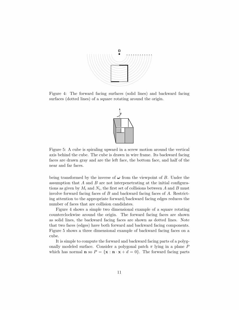
0

Figure 4: The forward facing surfaces (solid lines) and backward facingsurfaces (dotted lines) of a square rotating around the origin.

Figure 5: A cube is spiraling upward in a screw motion around the verticalaxis behind the cube. The cube is drawn in wire frame. Its backward facingfaces are drawn gray and are the left face, the bottom face, and half of thenear and far faces.

being transformed by the inverse of ω from the viewpoint of B. Under theassumption that A and B are not interpenetrating at the initial configura-tions as given by Mi and Ni, the first set of collisions between A and B mustinvolve forward facing faces of B and backward facing faces of A. Restrict-ing attention to the appropriate forward/backward facing edges reduces thenumber of faces that are collision candidates.

Figure 4 shows a simple two dimensional example of a square rotatingcounterclockwise around the origin. The forward facing faces are shownas solid lines, the backward facing faces are shown as dotted lines. Notethat two faces (edges) have both forward and backward facing components.Figure 5 shows a three dimensional example of backward facing faces on acube.

It is simple to compute the forward and backward facing parts of a polyg-onally modeled surface. Consider a polygonal patch π lying in a plane Pwhich has normal n so P = x : n · x + d = 0. The forward facing parts

11

of P satisfy ω(x) · n ≥ 0. Using (3), we have

ω(x) · n = (θj × x) · n + gj · n = (θn × j) · x + (gj · n).

If θn×j is zero, ω(x)·n is constant, equal to gj·n, and, depending on its sign,the plane P is either everywhere forward facing or everywhere backwardfacing. Otherwise ω(x) · n = 0 defines a plane Q, with normal directionθn× j. Since n · (n× j) = 0, Q is perpendicular to P , so Q and P intersectin a line L which splits P into forward facing and backward facing parts.The patch π, if it is intersected by L, splits into two polygonal subpatches,one forward facing and the other backward. The subpatches are computedby clipping the patch against the plane Q.

When computing forward and backward facing faces, there is the ad-ditional complication that some polygons have to be “doppeled” (i.e., pro-jected to the collision screen twice) in order to not miss any collisions. Dop-peling will be discussed in Section 8. It is logically distinct from the processof culling back faces, but is implemented by our algorithm at the same time.

4.3 An error estimate

In many cases, the assumption of screw motion is not completely correct.We can justify the use of screw motion by three arguments. (See [49] formore arguments for using screw motion.) First, the assumption of screwmotion is a priori no worse than many other assumptions. One might thinkthat a better assumption would be to let each object rotate on its own axis,but this assumption is also often incorrect, since physically moving bodiesdo not in general rotate on a fixed axis (c.f. [20]). Second, screw motionshave very nice properties such as the constancy of forward facing surfaces,and the fact that the forward facing portion of a polygonal face is a polygon.For these reasons, the algorithm described in Sections 6-9 requires the useof screw motions. Third, the error introduced by screw motions turns outto be quite small. The actual error depends on the motions of the twobodies of course, but it can be adequately estimated by finding the errorunder the assumption that one body is stationary and the other is rotatingat a constant rate on a fixed axis. In this case the error is essentially thedifference between “lerping” and “slerping” (see [54]) since the only error isin the position of the center of masses. To quantify this, we compare themotion of a point moving on a straight line to its motion when rotatingaround the origin. (For instance, the center of mass would be moved in acircular arc by a screw motion.) Figure 6 shows the two paths from x to y.The total rotation angle is θ and the maximum distance from the circular

12

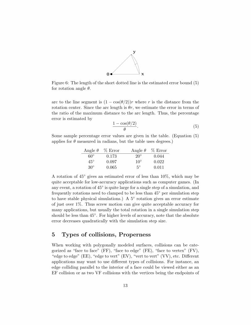
0 x

y

Figure 6: The length of the short dotted line is the estimated error bound (5)for rotation angle θ.

arc to the line segment is (1 − cos(θ/2))r where r is the distance from therotation center. Since the arc length is θr, we estimate the error in terms ofthe ratio of the maximum distance to the arc length. Thus, the percentageerror is estimated by

1 − cos(θ/2)θ

. (5)

Some sample percentage error values are given in the table. (Equation (5)applies for θ measured in radians, but the table uses degrees.)

Angle θ % Error Angle θ % Error60 0.173 20 0.04445 0.097 10 0.02230 0.065 5 0.011

A rotation of 45 gives an estimated error of less than 10%, which may bequite acceptable for low-accuracy applications such as computer games. (Inany event, a rotation of 45 is quite large for a single step of a simulation, andfrequently rotations need to clamped to be less than 45 per simulation stepto have stable physical simulations.) A 5 rotation gives an error estimateof just over 1%. Thus screw motion can give quite acceptable accuracy formany applications, but usually the total rotation in a single simulation stepshould be less than 45. For higher levels of accuracy, note that the absoluteerror decreases quadratically with the simulation step size.

5 Types of collisions, Properness

When working with polygonally modeled surfaces, collisions can be cate-gorized as “face to face” (FF), “face to edge” (FE), “face to vertex” (FV),“edge to edge” (EE), “edge to vert” (EV), “vert to vert” (VV), etc. Differentapplications may want to use different types of collisions. For instance, anedge colliding parallel to the interior of a face could be viewed either as anEF collision or as two VF collisions with the vertices being the endpoints of

13

P

A

B

n

`A

`B

ϕ > 0 P

A

B

n`A

`B

ϕ < 0

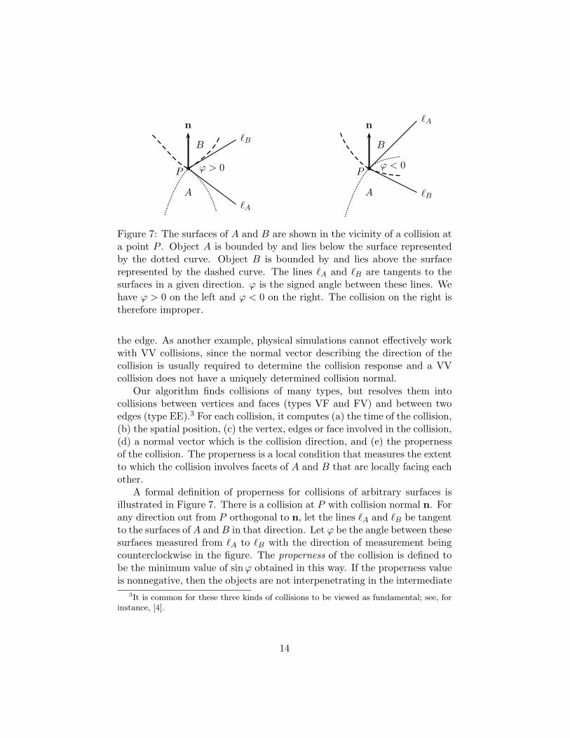
Figure 7: The surfaces of A and B are shown in the vicinity of a collision ata point P . Object A is bounded by and lies below the surface representedby the dotted curve. Object B is bounded by and lies above the surfacerepresented by the dashed curve. The lines `A and `B are tangents to thesurfaces in a given direction. ϕ is the signed angle between these lines. Wehave ϕ > 0 on the left and ϕ < 0 on the right. The collision on the right istherefore improper.

the edge. As another example, physical simulations cannot effectively workwith VV collisions, since the normal vector describing the direction of thecollision is usually required to determine the collision response and a VVcollision does not have a uniquely determined collision normal.

Our algorithm finds collisions of many types, but resolves them intocollisions between vertices and faces (types VF and FV) and between twoedges (type EE).3 For each collision, it computes (a) the time of the collision,(b) the spatial position, (c) the vertex, edges or face involved in the collision,(d) a normal vector which is the collision direction, and (e) the propernessof the collision. The properness is a local condition that measures the extentto which the collision involves facets of A and B that are locally facing eachother.

A formal definition of properness for collisions of arbitrary surfaces isillustrated in Figure 7. There is a collision at P with collision normal n. Forany direction out from P orthogonal to n, let the lines `A and `B be tangentto the surfaces of A and B in that direction. Let ϕ be the angle between thesesurfaces measured from `A to `B with the direction of measurement beingcounterclockwise in the figure. The properness of the collision is defined tobe the minimum value of sinϕ obtained in this way. If the properness valueis nonnegative, then the objects are not interpenetrating in the intermediate

3It is common for these three kinds of collisions to be viewed as fundamental; see, forinstance, [4].

14

vicinity of the collision point P . Negative values, between -1 and 0, indicatethat A and B are interpenetrating in the intermediate vicinity of P ; in thiscase the collision is improper. A negative properness value close to zeroindicates the collision is only slightly improper. For objects with smoothsurfaces, the maximum properness is zero since the surfaces will be tangentat a proper collision of smooth surfaces.

Because of the constancy of the values n ·ω(x) under the screw motion,the properness of a collision does not depend on the time of the collision.Instead the properness can be calculated from just the geometry of the twobodies in the neighborhood of the colliding points.

Properness is defined using the sine function since this allows using dotproducts to efficiently calculate the properness for polygonal surfaces. Theuse of the sine function is not particularly important since the only usemade of properness values is to decide, based on a fixed threshold, whetherto discard a potential collision. For example, we could use ϕ instead of sinϕand this would be equivalent if the threshold were changed appropriately.

For an FV collision (face f of body A against vertex v of body B),the collision normal is the unit normal n pointing outward from f . Letthe vertex have degree d, and let e1, e2, . . . , ed be the unit vectors pointingfrom v along its d adjacent edges. In order for the collision to be proper, itis necessary that ei · n ≥ 0. The properness of the collision is minei · n.

For an EE collision, let eA and eB be unit vectors along the two collidingedges, which are assumed to not be parallel. The collision normal n is a unitvector in the direction ±eA × eB. The sign of n is chosen so as to pointfrom body A towards body B; this done by choosing the sign to maximizethe value (7) below. Let nA,1 be the normal of the face on the left side of eA

and nA,2 be the normal of the face on the right side (by “left” and “right”we mean from the point of view of someone outside A traversing the edgein the direction eA). Define nB,1 and nB,2 similarly. The properness valueof a proper EE collision can be shown to equal

||eA×eB||·min(n×eA)·nA,1,−(n×eA)·nA,2,−(n×eB)·nB,1, (n×eB)·nB,2.(6)

But in practice, our algorithm uses

min(n× eA) ·nA,1,−(n× eA) ·nA,2,−(n× eB) ·nB,1, (n× eB) ·nB,2 (7)

instead of the true properness — this makes essentially no difference tothe operation of the algorithm since the properness of EE edges is neverused for any algorithmic purpose. We will not prove the correctness of theformula (6) except to note that it is easy to check that both (6) and (7)

15

are equal to the properness when the edges are perpindicular. It is alsoeasy to check that (6) and (7) are positive for proper collisions and negativefor improper collisions. We exclude the degenerate case of parallel edgescolliding: although these kinds of collisions could be proper, we never returnthem as collisions; instead they generate EV and VE collisions.

Our collision detection algorithm first identifies VV, EV, VE, EE, VF,and FV collisions. These are then resolved into VF, FV, and EE collisions.EE collisions are remain unchanged. The EV (resp., VE) collisions areresolved into FV (resp., VF) collisions by choosing one of the two facesadjacent to the edge as the collision face, namely the one that maximizes theproperness value. Each VV collision is resolved into an FV or VF collision:the algorithm considers each possible collision of one of the vertices againstone of the faces adjacent to the other vertex, and chooses a vertex-face pairthat maximizes the properness.

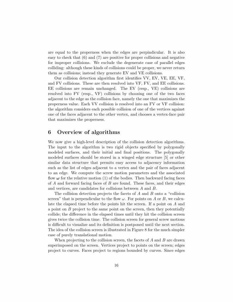
6 Overview of algorithms

We now give a high-level description of the collision detection algorithms.The input to the algorithm is two rigid objects specified by polygonallymodeled surfaces, and their initial and final positions. The polygonallymodeled surfaces should be stored in a winged edge structure [5] or othersimilar data structure that permits easy access to adjacency informationsuch as the list of edges adjacent to a vertex and the pair of faces adjacentto an edge. We compute the screw motion parameters and the associatedflow ω for the relative motion (1) of the bodies. Then backward facing facesof A and forward facing faces of B are found. These faces, and their edgesand vertices, are candidates for collisions between A and B.

The collision detection projects the facets of A and B onto a “collisionscreen” that is perpendicular to the flow ω. For points on A or B, we calcu-late the elapsed time before the points hit the screen. If a point on A anda point on B project to the same point on the screen, then they potentiallycollide; the difference in the elapsed times until they hit the collision screengives twice the collision time. The collision screen for general screw motionsis difficult to visualize and its definition is postponed until the next section.The idea of the collision screen is illustrated in Figure 8 for the much simplercase of purely translational motion.

When projecting to the collision screen, the facets of A and B are drawnsuperimposed on the screen. Vertices project to points on the screen; edgesproject to curves. Faces project to regions bounded by curves. Since edges

16

Screen

B

x y

t2 t4

A

u v

0 t1 t3

Figure 8: Two nonconvex objects A and B are moving horizontally. A ismoving leftward and B rightward, both at the same speed. A vertical col-lision screen is on the left and all four labeled points project orthogonallyto the same point on the screen. The horizontal axis measures the time fora point on A or B to hit the screen. Subtracting the times for two pointsof A and B gives twice the time until they collide. For instance, v will hitthe screen in time t3, and x hit the screen at t2 time units in the past. Thetwo points will collide at time (t3 − t2)/2 in the future. On the other hand,t1 < t2, so u and x appear to have collided at (t2 − t1)/2 time in the past.

project only to curves, not to straight lines, the algorithm approximates theprojected edges by a series of straight line segments that closely match thecurve. Wherever two projections of edges of A and B intersect, there is apotential EE collision. Likewise, wherever there is a projection of a vertexof A (resp. B) that lies in a projection of a face of B (resp. A), there isa potential VF (resp. FV) collision. When a point of A and a point of Bproject to a common point on the screen, there is a potential VV collision.Finally, if a vertex from one body projects onto the projection of an edgefrom the other body, there is a potential EV or VE collision.

For each potential collision, we find the preimages of the collision on theobjects A and B. We view B as being transformed by the screw motionand A as being transformed by the negative of the screw motion flow, andcalculate the times required for the point on A and the point on B to reachthe screen. Then one half the difference in times gives the collision time forthis potential collision. If a collision time is not in the interval [0, 1], thepotential collision is discarded and not considered further. The algorithmthen computes the properness of the remaining potential collisions. Allcollisions which are not too improper are reported as collisions.

The version of the algorithm we have implemented uses a screen thatconsists of pixels that hold information about all the facets that projectonto the pixel. In this approach, each backward (resp., forward) facingvertex of body A (resp. B) is projected to a pixel on the screen, and each

17

appropriately facing edge is drawn as one or more pixels on the screen.Each pixel may hold information from multiple vertices and edges. Thepixels holding edge information also hold information about the adjacentfaces, and this information is used to detect when vertex pixels potentiallycollide with faces.

The pixel-based approach is not the only possibility. An alternate methodwould treat the projection of the vertices as actual points, and the projec-tions of edges as curves (perhaps approximated by straight line segments),and then use techniques of [28] to determine what faces are intersected byvertices of the other body, and what edges from one body intersect edgesfrom the other body. The method could be made quite fast, although it is alittle more prone to roundoff errors causing discrepancies in the interpene-tration status from one simulation step to the next. It would be interestingto see it fleshed-out and implemented, but this has not been done yet.

7 Projection to the collision screen

The collision screen spirals around the screw rotation axis in a complicatedway. The pixels on the collision screen are indexed with pairs 〈r, h〉. Ther value is the radius, namely, the distance from the rotation axis. For a fixedvalue of r, the h value (“h” stands for “height”) measures distances alonga spiral which is perpendicular to the velocity flow of points at radius r.Points on objects A and B can collide only if they project to the same 〈h, r〉pixel on the screen.

Figure 9 illustrates the collision screen for a screw motion with param-eters g and θ and rotation axis the y-axis. The cylinder in the figure hasradius r and is centered on the rotation axis. The thick lines that spiralupward are the velocity flow of the screw motion. The dotted spiraling lineis the intersection of the collision screen and the cylinder: this line is at rightangles to the flow lines. This line is the h axis and one of the flow lines ischosen as the t axis. (Our convention has been to choose the t and h axesso that they intersect at the positive z axis.)

A point C at 〈x, y, z〉 is assigned coordinates 〈r, h〉 on the collision screenand a time value t. The t value is the time at which the point impacts thecollision screen and 〈r, h〉 is the position on the collision screen. Since theflow lines wrap around the cylinder, the choice of h and t is not unique. Forthis reason, some points need to be projected to more than a single pointon the projection screen; this is called “doppeling”.

The second part of Figure 9 shows the geometry for the calculation of

18

r

h

0

0

y

ϕ

D = 〈rθ, g〉g

rθ

h

t

C = 〈ϕ, y〉

E

F

Figure 9: The thick lines in both figures show the velocity flow. The dottedline in the left figure is the intersection of the collision screen with the pointsat distance r from the rotation axis. The figure on the right shows the planethat wraps around the cylinder. The y-axis points up as usual. The ϕ axismeasures azimuth and points rightward in the plane. The h and t values fora point C is found by projecting to E and F on the h- and t-axes.

r, h, and t. The cylinder for r =√

x2 + y2 has been unwrapped into aflat plane. Then ϕ = arctan(x/z) is the angle of the point C relative tothe yz-plane. Thus 〈r, ϕ, y〉 are cylindrical coordinates for C. The vector−→0D shows the net screw motion in a unit period of time. The time axis(t-axis) is coordinatized so that 0 is at t = 0 and D at t = 1. The h-axis isperpendicular to this flow. Note that the slope of the h-axis, like the slopeof the t-axis, depends on r. The point C, at 〈ϕ, y〉, is projected orthogonallyto the h- and t-axes. The h-coordinate of C is equal the distance ||0E||, andthe t-coordinate of C is equal to ||0F ||/||0D||. By similar triangles, the hand t-coordinates of C are

h =y · rθ − ϕ · g√

g2 + r2θ2and t =

y · g + ϕ · rθg2 + r2θ2

.

The time t for the point E on the screen to reach C can be positive ornegative. The value of ϕ was set with the multivalued arctangent function;by default, this puts ϕ in the interval [−π, π] and thereby uniquely deter-mines h and t. However, when doppeling, ϕ will get values outside the range[−π, π].

For a point that lies on the rotation axis, r = 0 and the ϕ value isundefined. However, we can still use the above formulas for h and t, withϕ = 0, so that h = 0 and t = y/g for such points.

A screw motion with θ = 0 is just a translation. Although the aboveconstruction still works for θ = 0, it is easier to just orthogonally project to

19

the collision screen. This case is further simplified by the fact that straightedges project to straight lines on the screen.

8 Doppeling

Recall that θ denotes the total rotation of the screw motion, whereas ϕ isused for cylindrical coordinates of points. As an example, suppose θ = 20,and consider a point u on object B which has ϕ value equal to 10. As Bmoves, the value of ϕ of the point u increases up to 10 + θ = 30. Thus,the point u can potentially collide with a point v on the stationary object Aonly if the ϕ value for v is between 10 and 30.

A more problematic case is when u has ϕ = 170. Then u may collidewith points v on A that have ϕ value between 170 and 190. The problem isthat a point v with ϕ value greater than 180 (190, for example) is by defaultprojected to the collision screen using ϕ = −170 instead of ϕ = 190. Thesetwo choices for ϕ will, in general, project the point to different points on thecollision screen and give it different collision times t. On the other hand, wecannot just use ϕ = 190 for such points v. A point v with ϕ = −170 canpotentially collide with points u on B that have ϕ ∈ [−180,−170] or haveϕ ∈ [170, 180]. Thus, v must be projected twice to the collision screen,with both ϕ = −170 and ϕ = 190.

Thus, for general values of θ (and returning to using radians), for anypoint v of object A with ϕ value in the interval [−π,−π +θ], the point mustbe projected twice to the collision screen, once with ϕ and once with ϕ+2π.This works well as long as θ < π. (In any event, usually θ ≤ π/4 in orderto control the error from the screw motion, c.f. Section 4.3.) When a pointis twice projected, we call it a “doppeled” point.

As discussed in the next section, the collision detection algorithm worksby projecting, one-by-one, each polygonal face to the collision screen. A faceis projected as a series of edges. When projecting a face of A we must checkwhether it has any points that need to be doppeled. If so, the face’s edgesmust be modified appropriately to properly doppel portions of the edges.There are several cases to consider, but the main ones are shown in Figures10 and 11. In Figure 10, a polygonal face contains points that need to bedoppeled, but does not intersect the screw axis. The figure shows a topview, looking down the screw axis, and the polygon is seen to intersect boththe ϕ = ±π line and the ϕ = θ−π line. The polygon is split by adding newvertices E, F , G and H. Vertices G and H use the ϕ value π + θ, whereasvertices E and F use ϕ = −π. The single polygon is split into two polygons

20

zϕ = 0

ϕ = −πϕ = π + θ

0

B

C

E

FA

D

H

G

Figure 10: The polygon ABCD is replaced by the two polygons AEFDand BCGH.

zϕ = 0

ϕ = −πϕ = π + θ

G,0

B

C

FA

D

E

Figure 11: The polygon ABCD is replaced by the “polygon” GEBCDAF .

AEFD and BCGH, and both are projected to the collision screen.Figure 11 shows a polygon ABCD that intersects the screw rotation

axis and thus contains points that need to be doppeled. For this polygon,we create new vertices E, F , and G, with G the point where the polygonintersects the screw axis (usually, G is not the same as 0). Then, the polygonABCD is replaced by the “polygon” GEBCDAF : the edges around thispolygon bound a non-self-overlapping region on the collision screen since theϕ starts off at π+θ at E and monotonically decreases down to ϕ = −π at F .

The situation is similar for body B, but is simpler since doppeling isnot needed. However, we still need to take care of edges that cross over theϕ = ±π boundary. Projecting from body B uses exactly the same algorithmas for projecting from body A except that now θ is set equal to zero. Forexample, in the situation of Figure 10, when we work with body B and haveθ replaced by zero, the points E and H correspond to the same point on theedge of B, except that E has ϕ = −π and H has ϕ = +π.

21

9 Pixel-based algorithm implementation

This section outlines the pixel-based algorithm we have implemented. Theinput to the algorithm includes the initial and final positions (and orien-tations) as given by Ni, Nf , Mi and Mh. The resolution of the rasterizedcollision screen also must be specified. The resolution is specified in termsof a distance between pixels (the r and h values are discretized to this res-olution), as well as a resolution in time.

The algorithm first determines the screw motion parameters g and θ(see Section 4.1). The coordinate system is chosen so that the y-axis isthe rotation axis and so that the (bounding spheres of the) two objects lieas close to the xz-plane as possible. Based on the bounding spheres, weattempt to place the z-axis so that no doppeling will be needed. We alsodo a bounding spheres test by bounding the maximum and minimum r, hand t values for all points on A and on B and checking whether any collisionis possible. If not, the algorithm halts, reporting no collisions. Otherwise,all initial vertex positions, edge directions and face normals are computedin this coordinate system to save later re-computation.

The second step clips edges so that only forward (resp., backward) facesof B (resp., A) will be considered. The clipping is done separately for eachface of A and B. Whenever a face is clipped in a non-trivial way, twoof its edges are also clipped. Since each edge abuts two faces, this meanseach edge can be potentially split into three segments. In the same step,doppeling information is also recorded for each edge. Doppeling can furthersplit an edge into up to three segments. In addition, for doppeling of thetype as shown in Figure 10, a face may also need to be doppeled. Notethat doppeling creates new edges; these are called virtual edges (e.g., edgesGH and EF in Figure 10 and GE and FG in Figure 11). The result ofthe second step is a list of clipped edges, i.e., original object edges and(sub)edges generated by the clipping and doppeling. With each (sub)edge,we store information about (a) which original edge (if any) it is a subedgeof, (b) whether the edge is virtual, (c) the identity of its left and right facesif they are forward facing. (Sub)edges from B (resp., A) that do not haveany adjacent forward (resp., backwards) facing edge can be discarded.

The third step projects the (sub)edges to pixels in the collision screenspace, generating a list of pixel records. Each edge is considered separately.We find the r and h values of the edges’ endpoints, and the time t at whichthe endpoints contact the collision screen (as described in Section 7). Then,a divide and conquer scheme projects the whole edge to a curve formed ofpixels on the collision screen. This is done by projecting the midpoint of the

22

edge to the collision screen and recursively considering the first and secondhalves of the edge. The divide-and-conquer assumes that the positionalaccuracy in projecting to the pixel screen needs to be no better than thepixel size, and likewise that the time value need be no more accurate thanthe time resolution input value.4 Once these accuracies are achieved, oronce the line segments are only one pixel long, the rest of the projected edgeis filled in with a Bresenham algorithm. If successive pixels from an edgeproject to the same r value, they are combined into a single pixel record;this is done to reduce the number of pixel records that are needed — laterstages of the algorithm will always scan all pixels with the same r valueat once. Each projected pixel record contains its r value, its maximumand minimum h values, hmin and hmax, and its time value t. In addition,the pixel record holds information about which edge it comes from, aboutthe left and right adjacent (appropriately facing) faces, about the time-duration of the pixel (this is important for edges that hit the collision screensomewhat perpendicularly since the range of t values for the pixel could besubstantial), and whether it is the projection of a vertex of the body. Toaid later steps, we also store some redundant information with each pixel,including information about the slope and direction of the projection of theedge through that point.

In the fourth step, the pixels are sorted lexicographically, first bucket-sorted by their r value, and second shell-sorted by their hmin value. Wethen make a copy of the pixel arrays, and re-sort so that the copy is sortedlexicographically by r and then hmax. The pixels for body A and for body Bare kept separate. We also create a list of pixels from vertices of A and pixelsfrom vertices of B, still sorted by r and h.

The fifth step finds vertices of body A that project into the interior ofa face of body B. For each appropriate value of r, we scan the following inorder of increasing h values: (i) pixels from vertices of A and (ii) pixel recordsfrom B sorted by hmin, and (iii) pixel records from B sorted by hmax. Pixelsof type (ii) tell us when the projection of a face of B is entered; pixels oftype (iii) tell us when the projection of a face of B is exited. For pixelsof type (i), we record that the vertex is potentially colliding with all thecurrently entered faces of B. This process is repeated with the roles of Aand B reversed.

The sixth step finds places where the projection of an edge of A crosses orintersects the projection of an edge of B. For this, pixel records are scannedlexicographically. Every time a pixel is found where two non-virtual edges

4This is the only place where the time resolution value is used.

23

cross, we store information about the potential intersection in a hash table.5

The edges’ pixels have time information, and if a pair of edges intersects atmultiple pixels (say if the edges coincide for a series of pixels), then we usethe pixel where the time until the potential collision is minimized. Some ofthese EE collisions involve endpoints. These are stored as EV, VE or VVcollisions in another hash table.

The fifth and sixth steps extracted all the potential EE, VV, EV, VE,FV and VF collisions. The final steps resolve these into EE, FV and VFcollisions. Collisions with properness value below a given threshold are dis-carded (the application has to determine the threshold; -0.1 works well fordriving game applications). For collisions between two edges, the informa-tion about the r, h and t values for the collision are obtained from the pixelrecords without further ado. For collisions between vertices and faces, the rand h position of the vertex is of course known. If the collision was resolvedfrom a VE, EV, or EE collision, then the pixel records give the collisiontime. However, if the collision is a VF or FV with the vertex colliding withthe interior of the face on the pixel screen, then the collision time cannot beobtained from just the pixel record. Instead, an iterative Newton method isused to find the point on the face that projects to the 〈r, h〉 position on thecollision screen where the vertex is projected, and from this, the collisiontime t is easily calculated. Convexity considerations prove that the Newtonmethod has fast guaranteed convergence.

The algorithm returns a list of potential EE, FV and VF collisions.Each collision record contains the following information: (a) the edges, orthe vertex and face, that have collided, (b) the time of the collision, (c) thespatial position and normal vector of the collision, and (d) its properness.

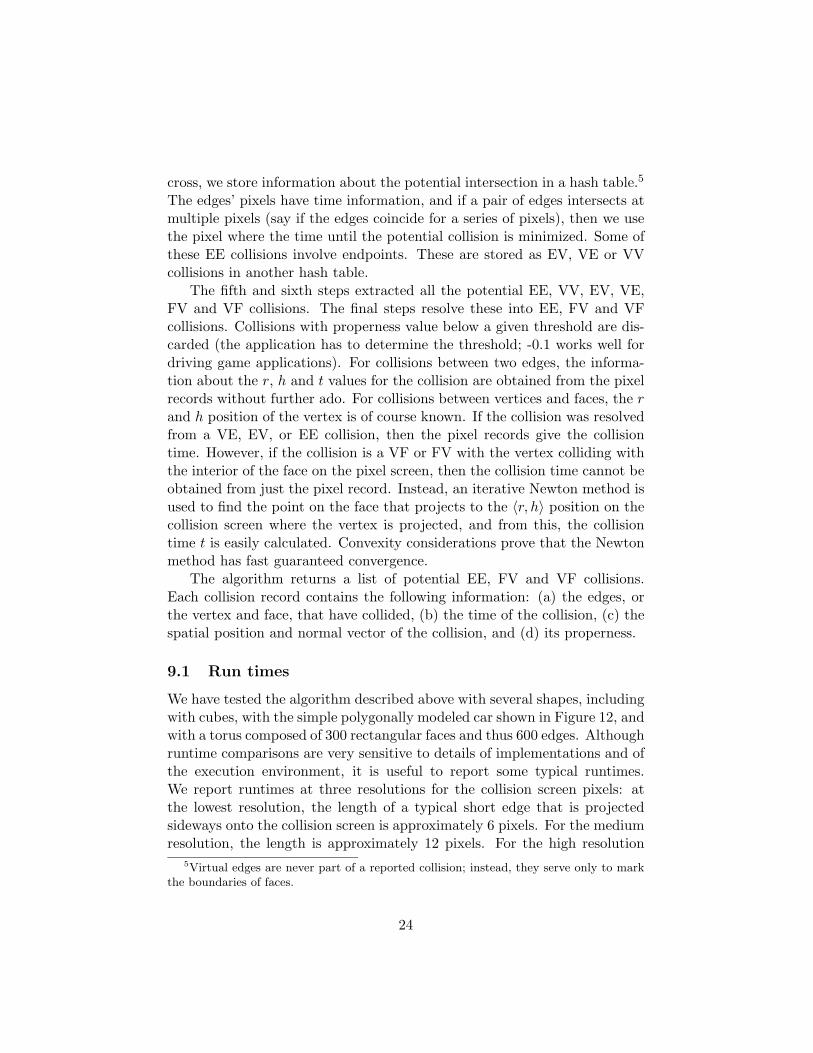
9.1 Run times

We have tested the algorithm described above with several shapes, includingwith cubes, with the simple polygonally modeled car shown in Figure 12, andwith a torus composed of 300 rectangular faces and thus 600 edges. Althoughruntime comparisons are very sensitive to details of implementations and ofthe execution environment, it is useful to report some typical runtimes.We report runtimes at three resolutions for the collision screen pixels: atthe lowest resolution, the length of a typical short edge that is projectedsideways onto the collision screen is approximately 6 pixels. For the mediumresolution, the length is approximately 12 pixels. For the high resolution

5Virtual edges are never part of a reported collision; instead, they serve only to markthe boundaries of faces.

24

the length is approximately 24 pixels. (The runtime is independent of theoverall size of the collision screen since pixel data is stored sparsely; instead,the runtime depends on the number of pixels occupied by features.) Theapproximate runtimes in microseconds are reported in the table below; testswere performed on a 2.4GHz Pentium IV. The first line is for a cube collidingwith a cube, the second line for a car versus car, and the third line for twocolliding complex tori.

low res medium res high resCubes: 56 µs 63 µs 77 µsCars: 109 µs 128 µs 170 µsTori: 2040 µs 2560 µs 3480 µs

Clearly there is a direct tradeoff between the runtime of the algorithm,and the resolution (and thereby the accuracy). Even the low resolutioncollisions work qualitatively quite well, although a close look will show thatthe collisions are only approximate. The choice of resolution is applicationdependent.

In general, for a fixed resolution, the runtime is expected to be approx-imately O(n log n) for the part of the algorithm that projects edges andvertices to pixels on the collision screen and sorts the pixels by their r and hvalues, since sorting O(n) records takes time O(n log n). The rest of thealgorithm is expected to take time approximately O(m) where m is thenumber of pairs of facets from A and B that project to the same pixel onthe screen. In the worst case, m = O(n2); indeed this is unavoidable, sincethere could be Ω(n2) many collisions that need to be reported. However, ifm ≈ n2, the runtime potentially could be reduced significantly if we modi-fied the algorithm so that it sorted pixels by time t in addition to by r and h.This change would allow the algorithm to work well with highly non-convexobjects, for instance screws threads in a screw hole.

It is difficult to make runtime comparisons with other published algo-rithms, since the bulk of these use extensive hierarchical methods to cullcollision testing, whereas our numbers above are for a full collision test.

We can make a fair comparison of runtime with the O(n2) runtime al-gorithms of Angel Studios. We have only been able to make very crude,approximate comparisons, but our algorithm appears to be close in speed toAngel Studios’s algorithms for a simple polygonal car, or perhaps slightlyslower. We should add that the Angel Studios’s algorithms have been greatlyoptimized over a period of years, whereas our own implementation is fairlypreliminary, thus it is likely that better implementations can improve our

25

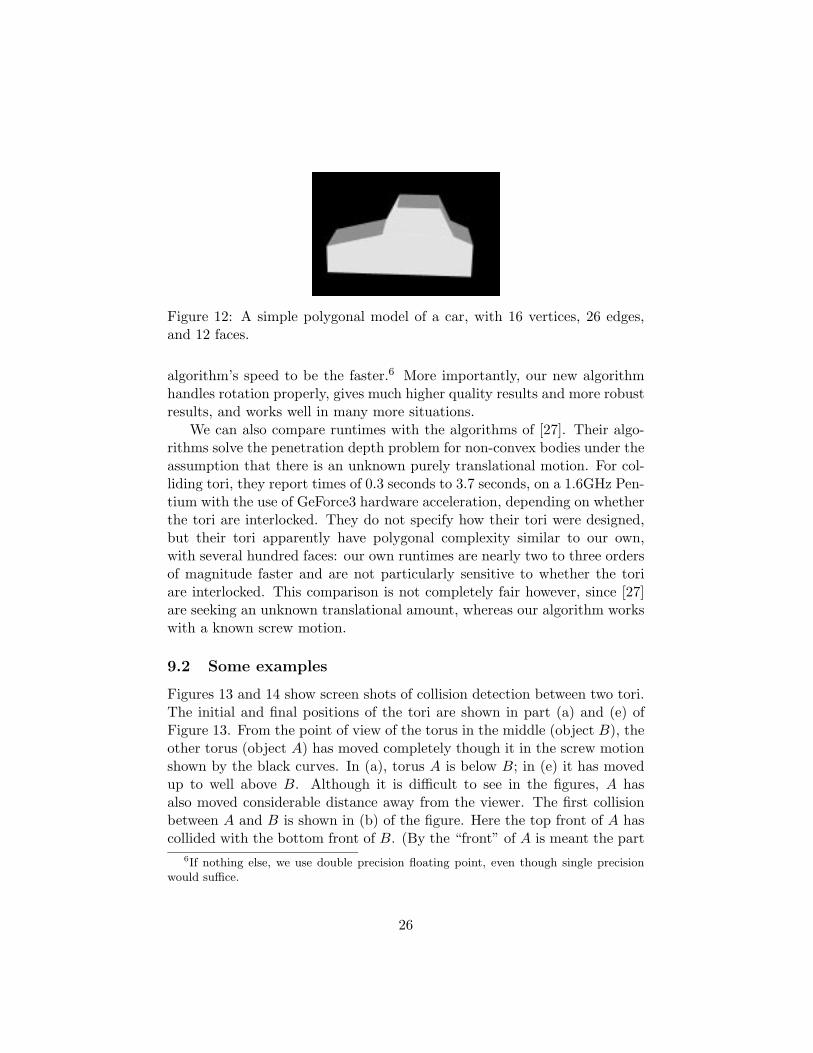
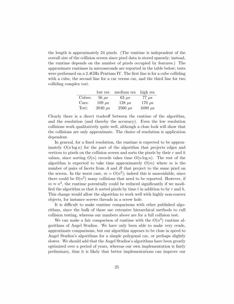
Figure 12: A simple polygonal model of a car, with 16 vertices, 26 edges,and 12 faces.

algorithm’s speed to be the faster.6 More importantly, our new algorithmhandles rotation properly, gives much higher quality results and more robustresults, and works well in many more situations.

We can also compare runtimes with the algorithms of [27]. Their algo-rithms solve the penetration depth problem for non-convex bodies under theassumption that there is an unknown purely translational motion. For col-liding tori, they report times of 0.3 seconds to 3.7 seconds, on a 1.6GHz Pen-tium with the use of GeForce3 hardware acceleration, depending on whetherthe tori are interlocked. They do not specify how their tori were designed,but their tori apparently have polygonal complexity similar to our own,with several hundred faces: our own runtimes are nearly two to three ordersof magnitude faster and are not particularly sensitive to whether the toriare interlocked. This comparison is not completely fair however, since [27]are seeking an unknown translational amount, whereas our algorithm workswith a known screw motion.

9.2 Some examples

Figures 13 and 14 show screen shots of collision detection between two tori.The initial and final positions of the tori are shown in part (a) and (e) ofFigure 13. From the point of view of the torus in the middle (object B), theother torus (object A) has moved completely though it in the screw motionshown by the black curves. In (a), torus A is below B; in (e) it has movedup to well above B. Although it is difficult to see in the figures, A hasalso moved considerable distance away from the viewer. The first collisionbetween A and B is shown in (b) of the figure. Here the top front of A hascollided with the bottom front of B. (By the “front” of A is meant the part

6If nothing else, we use double precision floating point, even though single precisionwould suffice.

26

(a) (b) (c)

(d) (e)

Figure 13: Two tori colliding. Torus A is moving away and upward. Torus Bis stationary.

most distant from the viewer; but the “front” of B is the part closest to theviewer.) In (c), the second collision is shown. Here the left top part of Ahas collided against the bottom part of B. In (d), the third collision is theright portion of the front of A colliding with the back inside of B. Thesethree collisions in Figure 13 are all the proper collisions that occur betweenA and B. Figure 14 shows the tori A and B drawn on the rasterized collisionscreen. The collision algorithm, in effect, finds points of intersection fromthe overlaid drawings.

10 Conclusions

We have described a robust algorithm for collision detection which gives goodapproximate results. The algorithm reports, all at once, all the potentialcollisions between two bodies over a period of time.

The robustness means that it is unlikely that the algorithm can becomeconfused about whether two bodies are interpenetrating. The approximate-ness does mean that sometimes the algorithm may report a collision when,in fact, the two bodies have only approached each other closely, and that,

27

Figure 14: The rasterized projections of tori A and B onto the collisionscreen. The (barely visible) short lines between pixels show the connectivityof projected edges. The dimensions of the collision screen is automaticallydetermined by the algorithm based on the r, h resolution levels and theextents of the objects; in this case, it has dimensions 28 × 50.

much more rarely, valid collisions where the bodies just barely interpene-trate can be missed, However, with care, the algorithm can be designed sothat, during the course of multiple simulation steps, two rigid bodies neverend up interpenetrating without a reported collision.7 One difficulty withrobustness is, in part, that two bodies might approach each other closely oreven interpenetrate slightly without generating a collision, and then, in thenext simulation step, as the screw motion may have completely changed, thebodies may appear to be already interpenetrated and to be moving in sucha way that no collision is occurring or has recently occurred. To make thecollision detection fully robust, the algorithm could be modified to find allcollisions where they approach to within a pixel’s resolution of each other.This would require a relatively simple change to (only) step six of the al-gorithm and would increase the runtime only modestly; however, it mightmean that the pixel resolution would need to be finer so as to not triggertoo many collisions when the bodies have not actually collided. A seconddifficulty with robustness arises from the assumption of relative screw mo-tion. It could happen that the relative screw motion of A and B showsno intersection, but A has a collision halfway through the time step with athird object. Then, if A and B are moved to their positions halfway throughthe time step, it may happen that they actually interpenetrate due to theirrelative motion not actually being a screw motion. (Similar problems arisein other scenarios, such as when interpenetrated objects are displaced to re-move the interpenetration.) One way to reliably avoid this kind of problem is

7This kind of robustness is very important for many applications, in particular, whentwo objects are in static contact, they frequently are almost touching or are barely inter-penetrated.

28

to keep track of the last time objects were known not to be interpenetrating,and check for collisions from these last known ‘good’ positions.

We expect that our algorithms can be improved or extended in severalways. First, there are several alternative implementations of the algorithmdescribed above, that might give a faster implementation. One such possi-bility was already mentioned at the end of Section 6. To mention another,we could have used a hash table to hold all pixels projected to the screenand thereby detect places where edges intersect or cross (instead of sortingand sequentially scanning). Second, as we noted above, the algorithm couldbe extended to handle highly non-convex objects, such a screw fitting intoa screw hole, by sorting pixels by time. Third, it would be interesting toextend our algorithm to other rigid shapes, say spheres or cylinders or, moregenerally, quadrics. Fourth, to handle highly complex objects, the algorithmshould be extended with hierarchical methods. Since the runtime is approx-imately O(n log n), it may be too slow for objects with many thousands offaces. Of course, a large speedup can be obtained with space partitioningmethods applied to (swept) bounding volumes to prune intersection test-ing. Another major speedup could also be obtained for complex objectsby using a lower resolution polygonal bounding volume that approximatesthe shape of the object. The lower resolution bounding volumes could beintersected with the screw motion algorithm and, where this indicate po-tential collisions, the higher resolution surfaces in just the regions of thepotential collisions could be collided, again with the screw motion method,for accurate collision detection.

A final natural question is whether the rasterized algorithm lends itselfwell to implementation on graphics hardware. Indeed, graphics hardwareacceleration has been successfully used for motion planning [33], for com-putation of Voronoi diagrams [23], and for hardware-based detection of in-terpenetration [2, 22, 32, 41, 48, 53]; see also [38]. The recent development(c.f. [42]) of sophisticated algorithms on graphics chips also gives hope thatgraphics hardware could accelerate our collision detection algorithm.

References

[1] P. K. Agarwal, L. J. Guibas, S. Har-Peled, A. Rabinovitch,

and M. Sharir, Penetration depth of two convex polytopes in 3D,Nordic J. Computing, 7 (2000), pp. 227–240.

[2] G. Baciu and W. S. K. Wong, Image-based techniques in a hybridcollision detector, IEEE Transactions on Visualization and Computer

29

Graphics, 9 (2003), pp. 254–271.

[3] D. Baraff, Fast contact force computation for nonpenetrating rigidbodies, Computer Graphics, 28 (1994), pp. 23–34. Proc. SIGGRAPH’94.

[4] , Rigid body simulation II—nonpenetration, 1997. Siggraph’97Course Notes.

[5] B. G. Baumgart, A polyhedral representation for computer vision, inProc. AFIPS Natl. Computer Conf., Vol. 44, 1975, pp. 589–596.

[6] J. W. Boyse, Interference detection among solids and surfaces, Com-munications of the ACM, 22 (1979), pp. 3–9.

[7] S. Cameron, A study of the clash detection problem in robotics, inProc. IEEE International Conf. on Robotics and Automation, 1985,pp. 488–493.

[8] , Collision detection by four-dimensional intersection testing,IEEE Transaction on Robotics and Animation, 6 (1990), pp. 291–302.

[9] , Enhancing GJK: Computing minimum and penetration dis-tances between convex polyhedra, in Proc. IEEE International Conf. onRobotics and Automation, 1997, pp. 3112–3117.

[10] J. Canny, Collision detection for moving polyhedra, IEEE Transactionson Pattern Analysis and Machine Intelligence, 8 (1986), pp. 200–209.

[11] A. Chatterjee and A. Ruina, A new algebraic rigid-body collisionlaw based on impulse space considerations, Journal of Applied Mechan-ics, 65 (1998), pp. 939–951.

[12] D. P. Dobkin, J. Hershberger, D. G. Kirkpatrick, and S. Suri,Computing the intersection-depth of polyhedra, Algorithmica, (1993),pp. 518–533.

[13] D. P. Dobkin and D. G. Kirkpatrick, Determining the separa-tion of preprocessed polyhedra — a unified approach, in Proc. 17thInternational Colloquium on Automata, Languages and Programming(ICALP), Lecture Notes in Computer Science #443, Springer Verlag,1990, pp. 400–413.

[14] J. Eckstein and E. Schomer, Dynamic collision detection in virtualreality applications, in Proc. 7th Intl. Conf. on Computer Graphics andVisualization and Interactive Digital Media, WSCG’9, 1999, pp. 71–78.

30

[15] S. Ehmann and M. C. Lin, Accelerated proximity queries betweenconvex polyhedra by multi-level voronoi marching, in Proc. InternationalConf. on Intelligent Robots and Systems, 2000, pp. 2101–2106.

[16] , Accurate and fast proximity queries between polyhedra usingconvex surface decomposition, Computer Graphics Forum, 20 (2001),pp. 500–510. Proc. Eurographics 2001.

[17] J. Erikson, L. J. Guibas, J. Stolfi, and L. Zhang, Separation-sensitive collision detection for convex objects, in Proc. ACM-SIAMSymp. on Discrete Algorithms (SODA), 1999, pp. 327–336.

[18] T. Giang, G. Bradshaw, and C. O’Sullivan, Complementaritybased multiple point collision resolution, in Prof. Fourth Irish Workshopon Computer Graphics (Eurographics, Ireland), 2003, pp. 1–8.

[19] E. G. Gilbert, D. W. Johnson, and S. S. Keerthi, A fast pro-cedure for computing the distance between objects in three-dimensionalspace, IEEE J. Robotics and Automation, RA-4 (1988), pp. 193–203.

[20] H. Goldstein, Classical Mechanics, Addison-Wesley, Reading, Mas-sachusetts, 1950.

[21] S. Gottschalk, M. C. Lin, and D. Manocha, OBBTree: A hier-archical structure for rapid interference detection, in Proc. ACM SIG-GRAPH’96, New York, 1996, ACM Press, pp. 171–180.

[22] N. K. Govindaraju, S. Redon, M. C. Lin, and D. Manocha,CULLIDE: Interactive collision detection between complex modelsin large environments using graphics hardware, in Proc. ACMSIGGRAPH-Eurographics Workshop on Graphics Hardware, 2003,pp. 25–32.

[23] K. E. Hoff III, T. Culver, J. Keyser, M. Lin, and D. Manocha,Fast computation of generalized Voronoi diagrams usings graphics hard-ware, Computer Graphics, 33 (1999), pp. 277–286. Siggraph’99.

[24] P. M. Hubbard, Collision detection for interactive graphics applica-tions, IEEE Transactions on Visualization and Computer Graphics, 1(1995), pp. 218–230.

[25] B. Kim and J. Rossignac, Collision prediction for polyhedra underscrew motions, in Proc. 8th ACM Symp. on Solid Modeling and Appli-cations, 2003, pp. 4–10.

31

[26] Y. J. Kim, M. C. Lin, and D. Manocha, DEEP: Dual space ex-pansion for estimating penetration depth between convex polytopes, inProc. IEEE International Conf. Robotics and Automation, 2002.

[27] Y. J. Kim, M. A. Otaduy, M. C. Lin, and D. Monocha, Fast pen-etration depth computation for physically-based animation, ACM Trans-actions on Graphics, (2002), pp. 23–31. SIGGRAPH 2002.

[28] D. G. Kirkpatrick, Optimal search in planar subdivision, SIAM J.Computing, 12 (1983), pp. 28–35.

[29] D. G. Kirkpatrick, J. Snoeyink, and B. Speckmann, Kineticcollision detection for simple polygons, International J. ComputationalGeometry, (2002), pp. 3–27.

[30] D. G. Kirkpatrick and B. Speckmann, Kinetic maintenance ofcontext-sensitive hierarchial representations for disjoint simple poly-gons, in Proc. 1st ACM Symp. on Computational Geometry, 2002,pp. 179–188.

[31] J. T. Klosowski, M. Held, J. S. B. Mitchell, H. Sowizral,

and K. Zikan, Efficient collision detection using bounding volumes ofk-DOPs, IEEE Transactions on Visualization and Computer Graphics,4 (1998), pp. 21–36.

[32] D. Knott and D. K. Pai, CInDeR: Collision and interference detec-tion in real-time using graphics hardware, in Proc. Graphics Interface,2003, pp. 73–80.

[33] J. Lengyel, M. Reichert, B. R. Donald, and D. P. Greenberg,Real-time robot motion planning using rasterizing computer graphicshardware, Computer Graphics, 24 (1990), pp. 327–335. SIGGRAPH’90.

[34] C. Lennerz, E. Schomer, and T. Warken, A framework for colli-sion detection and response, in Proc. 11th European Simulation Sym-posium and Exhibition (ESS’99), 1999, pp. 309–314.

[35] M. Lin, Collision Detection for Animation and Robotics, PhD thesis,U.C. Berkeley, 1993.

[36] M. C. Lin and J. F. Canny, Efficient algorithms for incremental dis-tance computation, in Proc. IEEE International Conference on Roboticsand Automation, 1991, pp. 1008–1014.

32

[37] M. C. Lin and S. Gottschalk, Collision detection between geometricmodels: A survey, in Proc. of IMA Conf. on Mathematics of Surfaces,1998, pp. 37–56.

[38] D. Manocha et al., Interactive geometric computations using graph-ics hardware, 2002. SIGGRAPH Course Notes #31.

[39] B. Mirtich, V-Clip: Fast and robust polyhedral collision detection,ACM Transactions on Graphics, 17 (1998), pp. 177–208.

[40] , Timewarp rigid body simulation, in Proc. ACM SIGGRAPH2000, 2000, pp. 193–200.

[41] K. Myszkowski, O. G. Okunev, and T. L. Kunii, Fast collisiondetection between complex solids using rasterizing graphics hardware,The Visual Computer, 11 (1995), pp. 497–512.

[42] T. J. Purcell, I. Buck, W. R. Mark, and P. Hanrahan, Raytracing on programmable graphics hardware, ACM Transactions onGraphics, 21 (2002), pp. 703–712. SIGGRAPH 2002.

[43] S. Redon, A. Kheddar, and S. Coquillart, An algebraic solutionto the problem of collision detection for rigid polyhedral objects, in Proc.IEEE International Conference on Robotics and Automation, vol. 4,2000, pp. 3733–3783.

[44] , CONTACT: Arbitrary in-between motions for collision detection,in Proc. 10th IEEE International Workshop on RObot and HumanInteractive Communication (ROMAN’2001), 2001, pp. 106–111.

[45] , Fast continuous collision detection between rigid bodies, Com-puter Graphics Forum, 21 (2002). Proc. Eurographics 2002.

[46] , Gauss’s least constraints principle and rigid body simulation, inProc. IEEE International Conference on Robotics and Automation,vol. 1, 2002, pp. 517–522.

[47] , Hierarchial back-face culling for collision detection, in Proc.IEEE/RSJ International Conference on Intelligent Robots and Systems,vol. 3, 2002, pp. 3036–3041.

[48] J. Rossignac, A. Megahed, and B. D. Schneider, Interactive in-spection of solids: Cross-sections and interferences, in SIGGRAPH’92,1992, pp. 353–360.

33

[49] J. J. Rossignac and J. J. Kim, Computing and visualizing pose-interpolating 3D motions, Computer Aided Design, 33 (2001), pp. 279–291.

[50] E. Schomer and C. Thiel, Efficient collision detection for movingpolyhedra, in Proc. 11th Annual ACM Symp. on Computational Geom-etry, 1995, pp. 51–60.

[51] J. M. Selig, Geometrical Methods in Robotics, Springer Verlag, NewYork, 1996.

[52] S. W. Shepperd, Quaternion from rotation matrix, Journal of Guid-ance and Control, 1 (1978), pp. 223–224.

[53] M. Shinya and M. C. Forgue, Interference detection through raster-ization, Journal of Visualization and Computer Animation, 2 (1991),pp. 131–134.

[54] K. Shoemake, Animating rotation with quaternion curves, ComputerGraphics, 19 (1985), pp. 245–254. SIGGRAPH’85.

[55] J. M. Snyder, A. R. Woodbury, K. Fleischer, B. Currin, and

A. H. Barr, Interval methods for multi-point collisions between time-dependent curved surfaces, Computer Graphics, 27 (1993), pp. 321–334.SIGGRAPH’93.

[56] G. Vanecek Jr., Back-face culling applied to collision detection ofpolyhedra, Journal of Visualization and Computer Animation, 5 (1994),pp. 55–63.

[57] B. von Herzen, A. H. Barr, and H. R. Zatz, Geometric collisionsfor time-dependent parametric surfaces, Computer Graphics, 24 (1990),pp. 39–48. SIGGRAPH’90.

34

List of Figures

Figure 1. Two interpenetrating squares. In the absence of informationabout the objects’ movement, the collision direction is ambiguous.

Figure 2. (a),(b). Two rectangles A and B have collided. Rectangle A onthe left is stationary. Rectangle B on the right is translating horizontallyleftward. (c) A polygon has collided with A while translating horizontally.

Figure 3. Determination of the point u on the rotation axis. The rotationaxis v is pointing straight up out of the figure. s = v × t/(2 tan(θ/2)) isperpendicular to the rotation axis.

Figure 4. The forward facing surfaces (solid lines) and backward facingsurfaces (dotted lines) of a square rotating around the origin.

Figure 5. A cube is spiraling upward in a screw motion around the verticalaxis behind the cube. The cube is drawn in wire frame. Its backward facingfaces are drawn gray and are the left face, the bottom face, and half of thenear and far faces.

Figure 6. The length of the short dotted line is the estimated errorbound (5) for rotation angle θ.

Figure 7. The surfaces of A and B are shown in the vicinity of a collisionat a point P . Object A is bounded by and lies below the surface representedby the dotted curve. Object B is bounded by and lies above the surfacerepresented by the dashed curve. The lines `A and `B are tangents to thesurfaces in a given direction. ϕ is the signed angle between these lines. Wehave ϕ > 0 on the left and ϕ < 0 on the right. The collision on the right istherefore improper.

Figure 8. Two nonconvex objects A and B are moving horizontally. A ismoving leftward and B rightward, both at the same speed. A vertical col-lision screen is on the left and all four labeled points project orthogonallyto the same point on the screen. The horizontal axis measures the time fora point on A or B to hit the screen. Subtracting the times for two pointsof A and B gives twice the time until they collide. For instance, v will hitthe screen in time t3, and x hit the screen at t2 time units in the past. Thetwo points will collide at time (t3 − t2)/2 in the future. On the other hand,t1 < t2, so u and x appear to have collided at (t2 − t1)/2 time in the past.

Figure 9. The thick lines in both figures show the velocity flow. The dottedline in the left figure is the intersection of the collision screen with the points

35

at distance r from the rotation axis. The figure on the right shows the planethat wraps around the cylinder. The y-axis points up as usual. The ϕ axismeasures azimuth and points rightward in the plane. The h and t values fora point C is found by projecting to E and F on the h- and t-axes.

Figure 10. The polygon ABCD is replaced by the two polygons AEFDand BCGH.

Figure 11. The polygon ABCD is replaced by the “polygon” GEBCDAF .

Figure 12. A simple polygonal model of a car, with 16 vertices, 26 edges,and 12 faces.

Figure 13. Two tori colliding. Torus A is moving away and upward.Torus B is stationary.

Figure 14. The rasterized projections of tori A and B onto the collisionscreen. The (barely visible) short lines between pixels show the connectivityof projected edges. The dimensions of the collision screen is automaticallydetermined by the algorithm based on the r, h resolution levels and theextents of the objects; in this case, it has dimensions 28 × 50.

36