collinsville solar thermal project - uq espace345800/energy_economics... · collinsville solar...

COLLINSVILLE SOLAR THERMAL PROJECT

ENERGY ECONOMICS

AND DISPATCH

FORECASTING

Final Report

Prepared for

RATCH-Australia Corporation

Collinsville solar thermal project: Energy economics and Dispatch forecasting

page 2

Chief Investigators

Professor Paul Meredith, Global Change Institute

Mr Craig Froome, Global Change Institute

Professor Hal Gurgenci, Queensland Geothermal Energy Centre of Excellence

Professor John Foster, School of Economics

Professor Tapan Saha, School of Information Technology and Electrical Engineering

Authors

Dr William Paul Bell, [email protected], Energy Economics and Management Group

Dr Phillip Wild, [email protected], Energy Economics and Management Group

Professor John Foster, [email protected], Energy Economics and Management Group

Energy Economics and Management Group

Postal address: School of Economics

The University of Queensland

St Lucia, Brisbane QLD 4072, Australia

Phone: +61 7 3346 0594 or +61 7 3365 6780

Fax: +61 7 3365 7299

Website: http://www.uq.edu.au/eemg/

Please cite this report as

Bell, WP, Wild, P, Foster, J, 2014, Collinsville solar thermal project: Energy economics and

Dispatch forecasting - Final report, The University of Queensland, Brisbane, Australia.

Final report – version 51 – 21 November 2014

Copyright

This work is licensed under a Creative Commons Attribution 4.0 International License.

mailto:[email protected]



http://www.uq.edu.au/eemg/

http://creativecommons.org/licenses/by/4.0/

http://creativecommons.org/licenses/by/4.0/


page 3

Preface

This combined Energy Economics and Dispatch Forecasting report is one of seven reports

evaluating the feasibility of a hybrid gas-concentrated solar power (CSP) plant using Linear

Fresnel Reflector (LFR) technology to replace the coal-fired power station at Collinsville,

Queensland, Australia. Table 1 shows the seven reports and the affiliation of the lead

authors.

Table 1: Collinsville feasibility study reports and their lead researcher groups and authors

Report Affiliation of the lead author

Yield forecasting (Bell, Wild & Foster 2014b) EEMG

*Dispatch forecasting (Bell, Wild & Foster 2014a) EEMG

*Energy economics (Bell, Wild & Foster 2014a) EEMG

Solar mirror cleaning requirements (Guan, Yu & Gurgenci 2014) SMME

Optimisation of operational regime (Singh & Gurgenci 2014b) SMME

Fossil fuel boiler integration (Singh & Gurgenci 2014a) SMME

Power system stability assessment (Shah, Yan & Saha 2014a) PESG

Yield analysis of a LFR based CSP by long-term historical data (Shah, Yan & Saha 2014b)

PESG

*Combined report

These reports are part of a collaborative research agreement between RATCH Australia and

the University of Queensland (UQ) funded by the Australian Renewable Energy Agency

(ARENA) and administered by the Global Change Institute (GCI) at UQ. Three groups from

different schools undertook the research: Energy Economics and Management Group

(EEMG) from the School of Economics, a group from the School of Mechanical and Mining

Engineering (SMME) and the Power and Energy Systems Group (PESG) from the School of

Information Technology and Electrical Engineering (ITEE).

EEMG are the lead authors for three of the reports. Table 2 shows the “Collinsville Solar

Thermal - Research Matrix” that was supplied by GCI to the researchers at EEMG for their

reports. We restructured the suggested content for the three reports in the matrix to provide

a more logical presentation for the reader that required combining the Energy Economics

and Dispatch Forecasting reports.


page 4

Table 2: Collinsville Solar Thermal - Research Matrix – EEMG’s components

Yield Forecasting Modelling and analysis of the solar output in order that the financial feasibility of the plant may be determined using a long-term yield estimate together with the dispatch model and the modelled long-term spot price.

Dispatch Forecasting Analysis of the expected dispatch of the plant at various times of day and various months would lead to better prediction of the output of the plant and would improve the ability to negotiate a satisfactory PPA for the electricity produced. Run value dispatch models (using pricing forecast to get $ values out). Output will inform decision about which hours the plant should run.

Energy Economics Integration of the proposed system into the University of Queensland’s Energy Economics Management Group’s (EEMG) existing National Electricity Market (NEM) models to look at the interaction of the plant within the NEM to determine its effects on the power system considering the time of day and amount of power produced by the plant. Emphasis to be on future price forecasting.

This Energy economics and dispatch forecasting report uses the results from our ‘Yield

forecasting’ report (Bell, Wild & Foster 2014b).

Justification for combining the Energy Economics and Dispatch Forecasting reports

The following paragraphs provide a detailed justification for combining the Energy

Economics and Dispatch Forecasting reports. This justification can be skipped by most

readers because the justification is most probably only of interest to ARENA and RATCH.

The matrix identifies improving the negotiation of a PPA as an important outcome of the

project. This objective is paramount given the failure of many renewable energy projects

stem from the failure to negotiate a suitable PPA. The negotiation of a PPA is required with

a purchaser of the electricity before banks or other intermediaries will provide finance for the

project. The financiers also require profit calculations for the lifetime of the plant before

financial approval is given, so the calculations are both essential to finalise the start of a

project and to aid in negotiating a PPA.

The revenue calculation requires both the prices and dispatch. However, the ‘Energy

Economics Report’ is to present prices and the ‘Dispatch Forecasting Report’ is to present

dispatch and PPA. Therefore, there would be duplication between the reports whichever

report presents the calculations. This duplication is unnecessary in a combined report. In

addition, the same EEMG ‘National Electricity Market (NEM)’ model produces both prices

and dispatch simultaneously, so it is more logical to discuss EEMG’s model and its outputs:

prices and dispatch, in the same report.

Furthermore, there is the failure of logic of presentation in the three-report format. We

calculated revenue from the prices and dispatch, so a logical presentation is to discuss the

prices and dispatch first then introduce the revenue calculations. This is not feasible in the

three-report format without duplication. Therefore, both clarity of exposition and removal of


page 5

duplication arguments make amalgamation of the ‘Energy Economics’ and ‘Dispatch

Forecasting’ reports sensible.

Doctor William Paul Bell

Research Fellow

Energy Economics and Management Group

The School of Economics

The University of Queensland


page 6

Executive Summary

1 Introduction

This report primarily aims to provide both dispatch and wholesale spot price forecasts for the

proposed hybrid gas-solar thermal plant at Collinsville, Queensland, Australia for its lifetime

2017-47. These forecasts are to facilitate Power Purchase Agreement (PPA) negotiations

and to evaluate the proposed dispatch profile in Table 3. The solar thermal component of

the plant uses Linear Fresnel Reflector (LFR) technology. The proposed profile maintains a

30 MW dispatch during the weekdays by topping up the yield from the LFR by dispatch from

the gas generator and imitates a baseload function currently provided by coal generators.

This report is the second of two reports and uses the findings of our first report on yield

forecasting (Bell, Wild & Foster 2014b).

2 Literature review

The literature review discusses demand and supply forecasts, which we use to forecast

wholesale spot prices with the Australian National Electricity Market (ANEM) model.

The review introduces the concept of gross demand to supplement the Australian Electricity

Market Operator’s (AEMO) “total demand”. This gross demand concept helps to explain the

permanent transformation of the demand in the National Electricity Market (NEM) region and

the recent demand over forecasting by the AEMO. We also discuss factors causing the

permanent transformation. The review also discusses the implications of the irregular ENSO

cycle for demand and its role in over forecasting demand.

Forecasting supply requires assimilating the information in the Electricity Statement of

Opportunities (ESO) (AEMO 2013a, 2014c). AEMO expects a reserve surplus across the

NEM beyond 2023-24. Compounding this reserve surplus, there is a continuing decline in

manufacturing, which is freeing up supply capacity elsewhere in the NEM. The combined

effect of export LNG prices and declining total demand are hampering decisions to transform

proposed gas generation investment into actual investment and hampering the role for gas

as a bridging technology in the NEM. The review also estimates expected lower and upper

bounds for domestic gas prices to determine the sensitivity of the NEM’s wholesale spot

prices and plant’s revenue to gas prices.

The largest proposed investment in the NEM is from wind generation but the low demand to

wind speed correlation induces wholesale spot price volatility. However, McKinsey Global

Institute (MGI 2014) and Norris et al. (2014a) expect economically viable energy storage

shortly beyond the planning horizon of the ESO in 2023-24. We expect that this viability will

not only defer investment in generation and transmission but also accelerate the growth in

off-market produced and consumed electricity within the NEM region.

2.1 Research questions

The report has the following overarching research questions:

What is the expected dispatch of the proposed plant’s gas component given the

plant’s dispatch profile and expected LFR yield?


page 7

What are the wholesale spots prices on the NEM given the plant’s dispatch profile?

The literature review refines the latter research question into five more specific research

questions ready for the methodology:

What are the half-hourly wholesale spots prices for the plant’s lifetime without gas as

a bridging technology?

o Assuming a reference gas price of between $5.27/GJ to $7.19/GJ for base-

load gas generation (depending upon nodal location;) and

o for peak-load gas generation of between $6.59/GJ to $8.99/GJ; and

o given the plant’s dispatch profile

What are the half-hourly wholesale spots prices for the plant’s lifetime with gas as a

bridging technology?

o Assuming some replacement of coal with gas generation

How sensitive are wholesale spot prices to higher gas prices?

o Assuming high gas prices are between $7.79/GJ to $9.71/GJ for base-load

gas generation (depending upon nodal location); and


What is the plant’s revenue for the reference gas prices?

How sensitive is the plant’s revenue to gas as a bridging technology?

How sensitive is the plant’s revenue to the higher gas prices?

What is the levelised cost of energy for the proposed plant?

3 Methodology

In the methodology section, we discuss the following items:

dispatch forecasting for the proposed plant;

supply capacity for the years 2014-47 for the NEM;

demand forecasting using a Typical Meteorological Year (TMY); and

wholesale spot prices calculation using ANEM, supply capacity and total demand

define three scenarios to address the research questions:

o reference gas prices;

o gas as a bridging technology; and

o high gas prices.

The TMY demand matches the solar thermal plant’s TMY yield forecast that we developed in

our previous report (Bell, Wild & Foster 2014b). Together, these forecasts help address the

research questions.

4 Results

In the results section we will present the findings for each research question, including

the TMY yield for the LFR and the dispatch of the gas generator given the proposed

dispatch profile in Table 3;

Average annual wholesale spot prices from 2017 to 2047 for the plant’s node for:

o Reference gas prices scenario from $18/MWh to $38/MWh

o Gas as a bridging technology scenario from $18/MWh to $110/MWh


page 8

o High gas price scenario from $20/MWh to $41/MWh

The combined plants revenue without subsidy given the proposed profile:

o Reference gas price scenario $36 million

o Gas as a bridging technology scenario $52 million

o High gas price scenario $47 million

5 Discussion

In the discussion section, we analyse:

reasons for the changes in the average annual spot prices for the three scenarios;

and

the frequency that the half-hourly spot price exceeds the Short Run Marginal Cost

(SRMC) of the gas generator for the three scenarios for:

o day of the week;

o month of the year; and

o time of the day.

If the wholesale spot price exceeds the SRMC, dispatch from the gas plant contributes

towards profits. Otherwise, the dispatch contributes towards a loss. We find that for both

reference and high gas price scenarios the proposed profile in Table 3 captures

exceedances for the day of the week and the time of the day but causes the plant to run at a

loss for several months of the year. Figure 14 shows that the proposed profile captures the

exceedance by hour of the day and Figure 16 shows that only operating the gas component

Monday to Friday is well justified. However, Figure 15 shows that operating the gas plant in

April, May, September and October is contributing toward a loss. Months either side of

these four months have a marginal number of exceedances. In the unlikely case of gas as a

bridging scenario, extending the proposed profile to include the weekend and operating from

6 am to midnight would contribute to profits.

We offer an alternative strategy to the proposed profile because the proposed profile in the

most likely scenarios proves loss making when considering the gas component’s operation

throughout the year. The gas-LFR plant imitating the based-load role of a coal generator

takes advantage of the strengths of the gas and LFR component, that is, the flexibility of gas

to compensate for the LFR’s intermittency, and utilising the LFR’s low SRMC. However, the

high SRMC of the gas component in a baseload role loses the flexibility to respond to market

conditions and contributes to loss instead of profit and to CO2 production during periods of

low demand.

The alternative profile retains the advantages of the proposed profile but allows the gas

component freedom to exploit market conditions. Figure 17 introduces the perfect day’s

yield profile calculated from the maximum hourly yield from the years 2007-13. The gas

generator tops up the actual LFR yield to the perfect day’s yield profile to cover LFR

intermittency. The residual capacity of the gas generator is free to meet demand when spot

market prices exceed SRMC and price spikes during Value-of-Lost-Load (VOLL) events.

The flexibility of the gas component may prove more advantageous as the penetration of

intermittent renewable energy increases.

6 Conclusion


page 9

We find that the proposed plant is a useful addition to the NEM but the proposed profile is

unsuitable because the gas component is loss making for four months of the year and

producing CO2 during periods of low demand. We recommend further research using the

alternative perfect day’s yield profile.

7 Further Research

We discuss further research compiled from recommendation elsewhere in the report.

8 Appendix A Australian National Electricity Market Model Network

This appendix provides diagrams of the generation and load serving entity nodes and the

transmission lines that the ANEM model uses. There are 52 nodes and 68 transmission

lines, which make the ANEM model realistic. In comparison, many other models of the NEM

are highly aggregated.

9 Appendix B Australian National Electricity Market Model

This appendix describes the ANEM model in detail and provides additional information on

the assumptions made about the change in the generation fleet in the NEM during the

lifetime of the proposed plant.


page 10

Contents

Preface ................................................................................................................................. 3

Executive Summary .............................................................................................................. 6

Figures ................................................................................................................................ 13

Tables ................................................................................................................................. 14

Equations ............................................................................................................................ 15

Abbreviations ...................................................................................................................... 16

1 Introduction .................................................................................................................. 19

2 Literature review .......................................................................................................... 20

2.1 Introduction ........................................................................................................... 20

2.2 Forecasting demand in the NEM for the lifetime of the proposed plant .................. 21

2.2.1 Short-run and long-run drivers for electricity demand ..................................... 21

2.2.2 Permanent transformation of demand: technological innovation redefining

demand .......................................................................................................... 22

2.2.3 Permanent transformation of demand: manufacturing decline ........................ 26

2.2.4 Permanent transformation of demand: smart meters ...................................... 28

2.2.5 Permanent transformation of demand: energy efficiency ................................ 29

2.2.6 Permanent transformation of demand: price awareness ................................. 32

2.2.7 Irregular cyclical transformation of demand: ENSO ........................................ 32

2.2.8 Over-forecasting bias and NSP profit correlation ............................................ 33

2.2.9 Demand Summary .......................................................................................... 33

2.3 Forecasting supply in the NEM for the lifetime of the proposed plant ..................... 35

2.3.1 Reserve deficit in Queensland and manufacturing decline .............................. 35

2.3.2 LNG export prices hampering gas generation’s potential as a bridging

technology ...................................................................................................... 36

2.3.3 WTG: Low demand to wind speed correlation inducing price volatility ............ 38

2.3.4 Energy storage deferring transmission infrastructure investment .................... 41

2.3.5 Supply Summary ............................................................................................ 41

2.4 Forecasting wholesale spot prices for the lifetime of the proposed plant using the

ANEM model ......................................................................................................... 43

2.4.1 The effect of the plant’s proposed dispatch profile on wholesale spot prices in

the NEM ......................................................................................................... 43

2.4.2 The effect of gas prices on wholesale spot prices ........................................... 43

2.5 Conclusion ............................................................................................................ 46

2.5.1 Research questions ........................................................................................ 46

3 Methodology ................................................................................................................ 47


page 11

3.1 What is the expected dispatch of the proposed plant’s gas component given the

plant’s dispatch profile and expected LFR yield? ................................................... 47

3.2 What are the half-hourly wholesale spots prices for the plant’s lifetime without gas

as a bridging technology? ...................................................................................... 48

3.2.1 Developing a TMY of market demand in the NEM for the lifetime of the

proposed plant ................................................................................................ 49

3.2.2 Forecasting supply for the lifetime of the proposed plant ................................ 52

3.3 What are the half-hourly wholesale spots prices for the plant’s lifetime with gas as a

bridging technology? ............................................................................................. 53

3.4 How sensitive are wholesale spot prices to higher gas prices? .............................. 53

3.5 What is the plant’s revenue for the reference gas prices? ..................................... 53

3.6 How sensitive is the plant’s revenue to gas as bridging technology? ..................... 54

3.7 How sensitive is the plant’s revenue to higher gas prices? .................................... 54

3.8 What is the Levelised Cost of Energy? .................................................................. 54

3.8.1 Total variable costs ......................................................................................... 55

3.8.2 Fixed costs ..................................................................................................... 56

3.8.3 Power Purchase Agreement Revenue Streams .............................................. 59

3.8.4 Half-hourly Operating Cash Flow .................................................................... 59

3.9 Conclusion ............................................................................................................ 60

4 Results ......................................................................................................................... 61

4.1 What is the expected TMY dispatch of the proposed plant given the plant’s dispatch

profile for hours of the week and expected TMY yield of the LFR? ........................ 61







4.6 How sensitive is the plant’s revenue to gas as bridging technology? ..................... 65



4.8.1 LCOE based on the yield forecast report ........................................................ 66

4.8.2 LCOE based on an inflated LFR yield ............................................................. 69

5 Discussion ................................................................................................................... 73

5.1 What is the expected dispatch of the proposed plant’s gas component given the

plant’s dispatch profile and expected LFR yield? ................................................... 73




page 12





5.6 How sensitive is the plant’s revenue to gas as bridging technology ....................... 81



5.9 Comparing scenarios by hour, month and day of week ......................................... 92

5.10 Imitating a coal baseload function or maximising the strengths and minimising the

weakness of LFR and CCGT technologies ............................................................ 94

6 Conclusion ................................................................................................................... 97

7 Further research .......................................................................................................... 98

7.1 Extending the reports TMY based years 2007-12 to include earlier years to remove

La Niña bias .......................................................................................................... 98

7.2 Wholesale spot price sensitivity to the proposed plant ........................................... 98

7.3 Solar water heaters replacing electric water heaters ............................................. 98

7.4 Poor correlation between wind speed and demand requiring more transmission (1) .

............................................................................................................................. 98

7.5 Poor correlation between wind speed and demand requiring more transmission (2) .

............................................................................................................................. 98

7.6 Small non-scheduled solar PV and WTG .............................................................. 98

7.7 Forthcoming enhancements in the next version of the ANEM model ..................... 99

8 Appendix A – Australian National Electricity Market Network ..................................... 100

9 Appendix B – Australian National Electricity Market Model ........................................ 106

9.1 Outline of the ANEM model ................................................................................. 106

9.2 Principal features of the ANEM model ................................................................. 107

9.2.1 Transmission grid characteristics in the ANEM model .................................. 107

9.2.2 Demand-side agents in the ANEM model: LSE’s .......................................... 108

9.2.3 Supply-side agents in the ANEM model: generators ..................................... 109

9.2.4 Passive hedging strategy incorporated in the ANEM model .......................... 110

9.3 DC OPF solution algorithm used in the ANEM model .......................................... 111

9.4 Practical implementation considerations .............................................................. 113

Acknowledgements ........................................................................................................... 121

References ....................................................................................................................... 122


page 13

Figures

Figure 1: 2013 NEFR annual NEM energy forecast ............................................................ 23

Figure 2: Comparing daily gross and net demand for 2007 & 2011 ..................................... 24

Figure 3: Six-year comparison of energy consumption ........................................................ 26

Figure 4: Intensity of Australian energy consumption .......................................................... 27

Figure 5 Shares of energy consumption and economic output 2005-06 .............................. 27

Figure 6: National Ownership of Air Conditioners by State .................................................. 30

Figure 7: Private residential approvals ................................................................................ 32

Figure 8: Mean annual SOI 1875-2013 ............................................................................... 33

Figure 9: Interconnectors on the NEM ................................................................................. 36

Figure 10: NEM existing and proposed projects by generation type (MW) .......................... 37

Figure 11: Average wholesale spot price in South Australia per MWh ................................. 39

Figure 12: Comparing Japan’s LNG and Europe’s and US’s natural gas prices .................. 44

Figure 13: Annual average wholesale spot prices for three scenarios on Collinsville’s node 64

Figure 14: By hour – number of half-hourly wholesale spot price exceedances of SRMC of

gas 2017-47 ...................................................................................................... 92

Figure 15: By month – number of half-hourly wholesale spot price exceedances of SRMC of

gas for 2017-47 ................................................................................................. 93

Figure 16: By day of week – number of half-hourly wholesale spot price exceedances of

SRMC of gas for 2017-47 ................................................................................. 94

Figure 17: Developing a perfect day’s yield profile from the years 2007-13 ........................ 95

Figure 18: Interconnectors on the NEM ............................................................................. 100

Figure 19: Stylised topology of QLD transmission lines and Load Serving Entities ............ 101

Figure 20: Stylised topology of NSW transmission lines and LSE ..................................... 102

Figure 21: Stylised topology of VIC transmission lines and Load Serving Entities ............. 103

Figure 22: Stylised topology of SA transmission lines and Load Serving Entities .............. 104

Figure 23: Stylised topology of TAS transmission lines and Load Serving Entities ............ 105


page 14

Tables

Table 1: Collinsville feasibility study reports and their lead researcher groups and authors ... 3

Table 2: Collinsville Solar Thermal - Research Matrix – EEMG’s components ...................... 4

Table 3: Proposed plant's total dispatch profile by hour of week ......................................... 19

Table 4: Regional reserve deficit timings ............................................................................. 25

Table 5: Projected population growth from 2006 to 2030 across the NEM .......................... 25

Table 6: Uneven projected household growth from 2006 to 2030 across the NEM .............. 31

Table 7: Projected household growth above population growth from 2006 to 2030 ............. 31

Table 8: Correlation of wind speed and demand ................................................................. 38

Table 9: South Australia’s wholesale spot prices ................................................................. 39

Table 10: Large non-scheduled wind farms included in modelling ....................................... 50

Table 11: Large non-scheduled wind farms excluded from modelling ................................. 50

Table 12: Large semi-scheduled wind farms included in modelling ..................................... 51

Table 13: Other large non-scheduled generation ................................................................ 52

Table 14: Years for the Typical Meteorological Months and Average daily Energy .............. 62

Table 15: The daily average energy from the LFR, gas and combined plant ....................... 62

Table 16: TMY's monthly distribution of the days of the week ............................................. 63

Table 17: Annual GWh Production and Capacity Factors associated with the given dispatch

profile ................................................................................................................ 63

Table 18: NPV Revenue for the three scenarios using 0.11 discount factor and 2017 base

year .................................................................................................................. 65

Table 19: Sensitivity of the plant's revenue to alternative scenarios .................................... 65

Table 20: Comparing capacity factors between this report and RAC (2014) ........................ 66

Table 21: Volume weighted average prices for node 3 for selected years and scenario ...... 67

Table 22: NPV Analysis for Various PPA Strike Prices Combinations by Scenario ............. 68

Table 23: Sweet spot analysis assuming PPA strike price for gas equals levelised cost of

gas component ................................................................................................. 69

Table 24: Inflated yield NPV Analysis for Various PPA Strike Prices Combinations by

Scenario ........................................................................................................... 70

Table 25: Original yield NPV Analysis for Various Average Price Levels ............................. 71

Table 26: Inflated yield NPV Analysis for Various Average Price Levels ............................. 71

Table 27: Price and Demand trends in Queensland 2010-14 .............................................. 72

Table 28: By day of the week - count of half-hourly wholesale spot price exceedance of short

run marginal cost for reference gas price .......................................................... 76

Table 29: By month - count of half-hourly wholesale spot price exceedance of SRMC for

reference gas price ........................................................................................... 78

Table 30: By hour - count of half-hourly wholesale spot price exceedance of SRMC for

reference gas price ........................................................................................... 79

Table 31: By day of the week - count of half-hourly wholesale spot price exceedance of

SRMC for gas as bridging technology ............................................................... 81

Table 32: By month - count of half-hourly wholesale spot price exceedance of SRMC for gas

as bridging technology ...................................................................................... 82

Table 33: By hour - count of half-hourly wholesale spot price exceedance of SRMC for gas

as bridging technology ...................................................................................... 84

Table 34: By day of the week - count of half-hourly wholesale spot price exceedance of

SRMC for high gas price ................................................................................... 86


page 15

Table 35: By month - count of half-hourly wholesale spot price exceedance of SRMC for high

gas price scenario ............................................................................................. 87

Table 36: By hour - count of half-hourly wholesale spot price exceedance of SRMC for high

gas price scenario ............................................................................................. 89

Table 37: Minimum stable operating capacity limits for coal plant, assumed operating time

and start-up cost status ................................................................................... 115

Table 38: Minimum stable operating capacity limits for baseload and intermediate gas plant,

assumed operating time and start-up cost status ............................................ 116

Equations

Equation 1: Demand - gross, scheduled and non-scheduled............................................... 24

Equation 2: Grossing-up total demand 2007-12 .................................................................. 49

Equation 3: Wholesale market profit .................................................................................... 54

Equation 4: Total revenue ................................................................................................... 54

Equation 5: Variable cost .................................................................................................... 54

Equation 6: Total variable costs .......................................................................................... 55

Equation 7: Short run marginal cost .................................................................................... 55

Equation 8: Capacity factor adjusted amortised total fixed costs per half-hour .................... 56

Equation 9: Annual fixed operations and maintenance costs per kW .................................. 57

Equation 10: Annual fixed operation and maintenance cost ................................................ 57

Equation 11: Fixed operation and maintenance cost per half-hour ...................................... 57

Equation 12: Capacity factor adjusted fixed operation and maintenance cost per half-hour 57

Equation 13: Capital cost per kW ........................................................................................ 57

Equation 14: Amortised annual capital cost per kW ............................................................ 58

Equation 15: Amortised annual capital costs ....................................................................... 58

Equation 16: Amortised capital cost per half hour ............................................................... 58

Equation 17: Capacity factor adjusted amortised capital cost per half-hour ......................... 58

Equation 18: PPA revenue for the gas component .............................................................. 59

Equation 19: PPA revenue for the solar component ............................................................ 59

Equation 20: Half-hourly PPA revenue from both the gas and solar components ................ 59

Equation 21: Half-hourly Operating cash flow (OCF) ........................................................... 59

Equation 22: Annual operating cash flow (AOCF) ............................................................... 60

Equation 23: Net Present Value of annual operating Cash flows less CAPEX .................... 60

Equation 24: ANEM’s objective function and constraints ................................................... 111


page 16

Abbreviations

ABS Australian Bureau of Statistics

AC Alternating Current

ACF Annual Capacity Factor

AEMC Australian Electricity Market Commission

AEMO Australian Energy Market Operator

AGL Australian Gas Limited

ANEM Australian National Electricity Market Model (from EEMG)

ARENA Australian Renewable Energy Agency

BRANZ Building Research Advisory New Zealand

BREE Bureau of Resources and Energy Economics

CCGT Combined Cycle Gas Turbine

CER Clean Energy Regulator

CSP Concentrated Solar Power

DC OPF Direct Current Optimal Power Flow

DNI Direct Normal Irradiance

E3 Equipment Energy Efficiency

EEMG Energy Economics and Management Group (at UQ)

ENSO El Niño Southern Oscillation

ESO Electricity Statement of Opportunities

GCI Global Change Institute

GDP Gross Domestic Product

GHG Green House Gas

GJ Gigajoule

IEA International Energy Agency

ISO Independent System Operator

ITEE Information Technology and Electrical Engineering (at UQ)

LCOE Levelised Cost of Energy


page 17

LFR Linear Fresnel Reflector

LMP Locational Marginal Price

LNG Liquid Natural Gas

LRET Large-scale Renewable Energy Target

LRMC Long Run Marginal Cost

LSE Load Serving Entity

MCE Ministerial Council on Energy

MEPS Minimum Energy Performance Standards

MGI McKinsey Global Institute

MVA Megavoltamperes

MW Megawatt

MWh Megawatt hour

NEFR National Electricity Forecast Report

NEM National Electricity Market

NFEE National Framework for Energy Efficiency

NGF National Generators Forum

NREL US National Renewable Energy Laboratory

NSP Network Service Provider

NSW New South Wales

NPV Net Present Value

OECD Organisation for Economic Cooperation and Development

OCGT Open Cycle Gas Turbine

PESG Power and Energy Systems Group (at UQ)

PPA Power Purchase Agreement

PV Photovoltaic

QLD Queensland

RAC RATCH Australia Corporation

SA South Australia


page 18

SAM Systems Advisor Model (from NREL)

SWH Solar Water Heater

SOI Southern Oscillation Index

SRMC Short Run Marginal Cost

LRMC Long Run Marginal Cost

TAS Tasmania

TMM Typical Meteorological Month

TMY Typical Meteorological Year

UQ University of Queensland

VIC Victoria

VO&M Variable Operation and Maintenance

VOLL Value-of-Lost-Load

WTG Wind Turbine Generator


page 19

1 Introduction

The primary aim of this report is to help negotiate a Power Purchase Agreement (PPA) for

the proposed hybrid gas-LFR plant at Collinsville, Queensland, Australia. The report’s wider

appeal is the techniques and methods used to model the NEM’s demand and wholesale spot

prices for the lifetime of the proposed plant.

To facilitate the PPA negotiations, this report produces the half-hourly dispatch of the plant’s

gas component and the associated half-hourly wholesale spot prices for the plant’s node on

National Electricity Market (NEM) given the yield from the plant’s solar thermal component

and a fixed total dispatch profile shown in Table 3. The total dispatch profile incorporates

both gas and solar outputs and differs between weekdays and weekends.

Table 3: Proposed plant's total dispatch profile by hour of week

Time Dispatch (MW)

Weekdays: 8am-10pm 30

Weekdays: 7am-8am ramp from 0 to 30

Weekends entire yield of the solar thermal component

The half-hourly yield profile for the solar thermal component of the plant is determined in our

previous report (Bell, Wild & Foster 2014b). Three profiles are utilised to help to negotiate a

PPA: solar thermal yield, gas dispatch and wholesale market spot price.

The executive summary provides an outline of the report.


page 20

2 Literature review

2.1 Introduction

This literature review helps us to develop the research question and inform the methodology

to address the research question. This report uses two research questions to express the

report’s research requirements shown in Table 2.




The literature review informs the development of forecasts for the National Electricity Market

(NEM) for the 30 year lifetime of the proposed new solar thermal plant from 1 April 2017 to

31 March 2047 (RAC 2013).

Section 1 discusses demand forecasting. Section 2 discusses supply forecasting. Section 3

discusses dispatch and wholesale spot price forecasting while developing supporting

research questions to investigate the interaction of the proposed plant with the NEM.

Section 3 also introduces the Australian National Electricity Market (ANEM) Model that this

report uses to calculate the dispatch and wholesale spot prices from the demand and supply

forecasts in Sections 2 and 3.


page 21

2.2 Forecasting demand in the NEM for the lifetime of the proposed plant

This section discusses forecasting demand for the lifetime of the proposed plant.

There has been an increase in demand for electricity for over two decades. However, more

recently, the Australian Electricity Market Operator (AEMO) has produced a number of

demand forecasts that have over projected demand and have missed the general declining

demand for electricity. This section focuses on reasons for AEMO’s over-forecasting to help

inform this report’s demand forecasting.

There are many countervailing trends in the demand for electricity. For instance, there is

uneven population growth across Australia, which will affect demand unevenly. The growth

in the uptake of air conditioners is nearing a plateau, which will reduce the rate of increase in

electricity demand. The price for electricity has increased rapidly over the last 10 years,

which may see people become sensitive to price, so a price elasticity of demand starts to

slow the rate of increase in demand. There are education campaigns to make people aware

of their electricity use, which will reduce the rate of increase. Additionally, there is the

ongoing shift in the economy from manufacturing to services, which will reduce demand

because manufacturing is the most energy intensive sector.

Section 1 discusses the short and long-term drivers for demand. Sections 2 to 6 discuss

structural changes to electricity demand that cause a permanent decrease in total demand.

Section 7 discusses the ENSO cycle that causes temporary changes in total demand.

Section 8 discusses the AEMO’s over-forecasting of electricity demand.

2.2.1 Short-run and long-run drivers for electricity demand

Yates and Mendis (2009, p. 111) consider short-run drivers for demand due to weather, for

instance in the short-run people can turn on fans or air conditions to meet changes in

weather conditions. Yates and Mendis (2009, p. 111) list the following short-run electricity

demand drivers:

weather – air temperature, wind speed, air humidity and radiation;

indoor environmental factors – indoor air temperature, wind speed and humidity;

time of the day;

day of the week;

holidays;

seasons;

durations of extreme heat days;

urban heat island effects;

utilisation of appliances;

person’s financial position; and

personal factors – clothing, physical activity and acclimatisation.

This report uses demand profiles from the years 2007-12, which incorporate all these short-

run drivers for demand. We create a typical meteorological year (TMY) demand profile using

the same twelve typical meteorological months (TMMs) derived in our yield report (Bell, Wild

& Foster 2014b). This process ensures consistency between the reports, so both demand

profile and yield profiles have consistent weather conditions.


page 22

Yates and Mendis (2009, p. 112) consider the following long-run drivers for demand:

climate change;

population growth, composition and geographic distribution;

real price of electricity;

the price of electricity relative to the price of gas;

economic growth;

real income and employment status;

interest rates;

renewal of building stock;

households and floor space per capita;

previous years consumption; and

commercial and industrial electricity use.

The AEMO's long-term forecasts incorporate these changes. Therefore, we could use the

AEMO’s forecasts to provide a growth rate for the TMY demand profile. However, the

AEMO forecasts present two problems: consistently over-forecasting total demand in recent

years and failure to cover the entire lifetime time of the proposed plant. Additionally, in the

long-run people can install solar PV, solar water heaters and more energy efficient

appliances and build more energy efficient housing. These have the effect of transforming

the shape of the demand profile. Norris et al. (2014a) discuss the transformative effect of

new technology changing the well-established accurate long-term predictions of electricity

demand into disarray.

The next section discusses extending the definition of demand to account for these changes

and the subsequent adjustment of the shape of the TMY demand profile.

2.2.2 Permanent transformation of demand: technological innovation redefining demand

Bell, Wild and Foster (2013) investigates the transformative effect of non-scheduled solar PV

and wind turbine generation (WTG) on total electricity demand. The motivation for our study

is a series of forecasts by the AEMO for increases in total demand but there is a continuing

reduction in total demand see Figure 1.


page 23

Figure 1: 2013 NEFR annual NEM energy forecast

(Source: AEMO 2013a)

A number of factors contribute to these poor predictions, including: the Australian economy’s

continued switch from industrial to service sector, improvements in energy efficiency, the

promotion of energy conservation, and mild weather induced by the La Niña phase of the

ENSO cycle reducing the requirement for air conditioning. Section 2.2.7 discusses the

ENSO cycle in more detail. Additionally, there is growing non-scheduled generation that is

meeting electricity demand.

However, the AEMO’s “Total demand” definition fails to account for non-scheduled

generation. AEMO (2012, sec. 3.1.2) defines the “Total Demand” in the following way.

“Total Demand” is the underlying forecast demand at the Regional Reference Node

(RRN) that is met by local scheduled and semi-scheduled generation and

interconnector imports after excluding the demand of local scheduled loads and that

allocated to interconnector losses.

“Total Demand” is used for the regional price calculations in Dispatch, Pre-dispatch

and Five-minute Pre-dispatch 5MPD, and to determine dispatch targets for

generating units.

Semi-scheduled wind farms are included in “Total Demand" but non-scheduled wind farms

are excluded.

0

50,000

100,000

150,000

200,000

250,000

300,000

An

nu

al

en

erg

y c

on

su

mp

tio

n (

GW

h)

Financial year

2013 High 2013 Medium 2013 Low Actuals

2012 High 2012 Medium 2012 Low


page 24

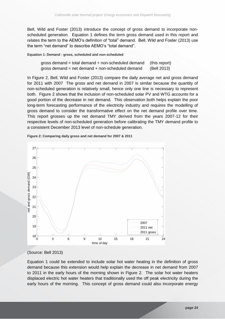
Bell, Wild and Foster (2013) introduce the concept of gross demand to incorporate non-

scheduled generation. Equation 1 defines the term gross demand used in this report and

relates the term to the AEMO’s definition of “total” demand. Bell, Wild and Foster (2013) use

the term “net demand” to describe AEMO’s “total demand”.

Equation 1: Demand - gross, scheduled and non-scheduled

gross demand = total demand + non-scheduled demand (this report)

gross demand = net demand + non-scheduled demand (Bell 2013)

In Figure 2, Bell, Wild and Foster (2013) compare the daily average net and gross demand

for 2011 with 2007 The gross and net demand in 2007 is similar because the quantity of

non-scheduled generation is relatively small, hence only one line is necessary to represent

both. Figure 2 shows that the inclusion of non-scheduled solar PV and WTG accounts for a

good portion of the decrease in net demand. This observation both helps explain the poor

long-term forecasting performance of the electricity industry and requires the modelling of

gross demand to consider the transformative effect on the net demand profile over time.

This report grosses up the net demand TMY derived from the years 2007-12 for their

respective levels of non-scheduled generation before calibrating the TMY demand profile to

a consistent December 2013 level of non-schedule generation.

Figure 2: Comparing daily gross and net demand for 2007 & 2011

(Source: Bell 2013)

Equation 1 could be extended to include solar hot water heating in the definition of gross

demand because this extension would help explain the decrease in net demand from 2007

to 2011 in the early hours of the morning shown in Figure 2. The solar hot water heaters

displaced electric hot water heaters that traditionally used the off peak electricity during the

early hours of the morning. This concept of gross demand could also incorporate energy

0 3 6 9 12 15 18 21 2418

19

20

21

22

23

24

25

26

27

time of day

net

and g

ross d

em

and (

GW

)

2007

2011 net

2011 gross


page 25

efficiency. Section 7.3 in further research discusses incorporating the effect of solar hot

water heating and energy efficiency on demand.

The McKinsey Global Institute (MGI 2014) expects the cost of solar PV installations to

continue to decrease. Further installation will further depress the midday depression in “total

demand” (net demand) in Figure 2. However, MGI (2013) and Norris et al. (2014a) expect

battery storage to become economically viable in 2025, perhaps even earlier given sudden

innovations. This timing is well within the lifetime of the proposed plant. Battery storage in

conjunction with non-scheduled generation allows further growth in gross demand with little

or no growth in “total demand”. Furthermore, the time shifting feature of battery storage is

likely to moderate both the midday depression and the evening peak in total demand shown

in Figure 2.

There are two consequences of the economic viability of battery storage for the proposed

plant: no growth in total demand post 2025 and a transformation of the relative profitability of

the LFR and gas components of the plant. The environment prior to battery storage

provides relatively higher profitability for the gas component than the LFR and vice versa.

The AEMO (2014d) expects the capacity of the current generation fleet sufficient to meet

any increase in total demand until after 2023, see Table 4, which is when battery storage is

expected to allow growth in gross demand without an increase in total demand. The only

exception is Queensland, which may have a reserve deficit in 2020-21. This is just short of

the period when MGI (2013) expect battery storage to induce no growth in total demand that

makes any new scheduled generation a very marginal proposition.

Table 4: Regional reserve deficit timings

Queensland NSW Victoria SA Tasmania

Reserve deficit timings 2020-21 Beyond 2022-23

Beyond 2022-23

Beyond 2022-23

Beyond 2022-23

(Source: AEMO 2014d)

At least three factors could account for the AEMO projecting shorter reserve deficit timing for

Queensland than the rest of the NEM: population growth, the production of liquefied natural

gas (LNG) and other mining activity. Consistent with the AEMO’s projection, Table 5 shows

the most likely percent growth in population across the NEM from 2006 to 2030 where the

ABS(2008) expects Queensland to have a relatively high expected population growth

compared to the rest of the NEM.

Table 5: Projected population growth from 2006 to 2030 across the NEM

Series B Qld NSW Vic SA Tas ACT NEM

State 57% 27% 36% 24% 14% 29% 36%

Capital city 57% 32% 41% 25% 22% 38%

Balance of state 57% 20% 20% 21% 8% 32%

(Source: ABS 2008)

However, Figure 2, in a quarterly update (AEMO 2014d) of the Electricity Statement of

Opportunities (ESO) (AEMO 2013a), shows the demand across the NEM continues to

decrease. This literature review discusses reasons for the poor forecast further. For


page 26

instance, Section 2.2.5 discusses energy efficiency and the switch to high density living that

will reduce “total demand” per capita. Additionally, Section 2.2.3 discusses the production of

liquefied natural gas in Queensland, the resources bubble and associated decline in

manufacturing that will also reduce “total demand” per capita.

Figure 3: Six-year comparison of energy consumption

(AEMO 2014d)

2.2.3 Permanent transformation of demand: manufacturing decline

Figure 4 shows that growth in energy consumption has remained below the growth in Gross

Domestic Product (GDP) and energy-intensity has been declining. Energy-intensity is the

ratio of energy used to activity in the Australian economy. Ball et al. (2011, p. 8) discuss

how declining energy-intensity is a worldwide phenomenon.

Shultz and Petchey (2011, p. 5) consider the decline in energy-intensity is due to two factors:

improving energy efficiency associated with technological advancement; and

shifting industrial structure toward less energy-intensive sectors.


page 27

Figure 4: Intensity of Australian energy consumption

(Source: Schultz & Petchey 2011, p. 5)

The improvement in energy efficiency is likely to continue. Figure 5 compares the

percentage share of economic output and of energy use for different industries.

Manufacturing is the most energy intensive industry and the service industry is one of the

least intensive industries. Mining is less energy intensive than manufacturing. Therefore,

the increase in the size of both service and mining industries and decrease in the size of the

manufacturing industry accounts for some of the decline in energy-intensity.

Figure 5 Shares of energy consumption and economic output 2005-06

(Source: Sandu & Syed 2008, p. 4)

There is a temporary increase in electricity demand from increased construction activity in

Queensland to establish the infrastructure ensuing from the resources bubble and more

specifically, to make the gas trains to liquefy natural gas (LNG) for export.

However, the resources bubble via the exchange rate mechanism accelerates the decline in

manufacturing. The bubble causes Australia’s exchange rate to appreciate. This


page 28

appreciation makes Australia’s manufactured exports relatively more expensive to buyers

overseas and makes manufactured imports relatively less expensive to buyers in the

domestic market. In addition, the gas price increases ensuing from the export of LNG will

further accelerate the decline of the manufacturing sector and, in turn, reduce “total” demand

for electricity.

The latest major manufacturing closures include:

car manufacturing in SA, NSW and VIC

Alcoa’s smelter and roll mills in VIC and NSW

These manufacturing industries are unlikely to return after the collapse of the resources

bubble because there are on-going moves toward more trade liberalisation. The

consequence is a persistent reduction in “total demand”. The reduction in “total demand”

caused by the manufacturing decline affects the NEM unevenly with NSW and VIC having

the largest declines in absolute terms.

Sections 2.2.3 and 2.3.2 discuss further the consequences of the resources bubble and LNG

export for the NEM and the proposed plant.

2.2.4 Permanent transformation of demand: smart meters

This section discusses how smart meters providing customers with dynamic pricing can help

customers reduce demand for electricity at peak times and increase public engagement in

energy conservation.

Smart meters allow retailers to collect high frequency data automatically on customers’

electricity usage and customers to monitor their own use of electricity. Smith and Hargroves

(2007) discusses the introduction of smart meters, the ensuing public engagement and the

substantial reduction in peak demand being achieved. Currently in Australia, the

requirement to meet peak demand drives transmission and distribution investment decisions.

This peak demand is usually between 3 pm and 6 pm in most ‘Organisation for Economic

Cooperation and Development’ (OECD) countries. Georgia Power and Gulf Power in Florida,

USA, have installed smart meters resulting in Georgia Power’s large customers reducing

electricity demand by 20-30 per cent during peak times and Gulf Power achieving a 41 per

cent reduction in load during peak times. Zoi (2005) reports on California’s experience of

tackling the growing demand for peak summer power using a deployment of smart meters

with a voluntary option for real time metering that uses lower tariffs during off peak times and

higher tariffs during peak times with a ‘critical peak price’ reserved for short periods when the

electricity system is really stressed. A key finding was a 12-35 per cent reduction in energy

consumption during peak periods. Moreover, most Californians have lower electricity bills

and 90 per cent of participants support the use of dynamic rates throughout the state.

Australia is slow in deploying smart meters, and Queensland is particularly slow, but the

deployment across the NEM within the lifetime of the proposed plant is a reasonable

expectation. Norris et al. (2014b) provide a cost-benefit justification for an Australian wide

rollout of a smart grid.


page 29

2.2.5 Permanent transformation of demand: energy efficiency

Improvements in energy efficiency are an ongoing process and expected to reduce “total”

demand in the NEM. However, the state based approach to energy efficiency has hampered

improvements. Nevertheless, during the lifetime of the plant more effective energy efficiency

policy and deployment is expected.

Hepworth (2011) reports how AGL and Origin Energy called for a national scheme rather

than state based schemes because compliance across the different states’ legislations is

costly. However the National Framework for Energy Efficiency (NFEE 2007) instituted by

the Ministerial Council on Energy (MCE) claims significant progress. But in a submission to

the NFEE (2007) consultation paper for stage 2, the National Generators Forum (NGF 2007)

comments on the progress since stage 1 of the NFEE: “Progress in improving the efficiency

of residential and commercial buildings can best be described as slow and uncoordinated,

with a confusion of very mixed requirements at the various state levels. … Activities in areas

of trade and professional training and accreditation, finance sector and government have

been largely invisible from a public perspective”. The NGF (2007) states that the proposals

for stage 2 are modest and lack coordination and national consistency. Therefore, there is

disagreement between the MCE and participants in the NEM over coordination in the NEM.

The star rating of appliances by Equipment Energy Efficiency (E3 2011) is an example of a

campaign that is visible and easy to understand, which is moot with some success and

addresses information asymmetry. As discussed, the introduction of smart meters and

flexible pricing has engaged customers in other countries. This public engagement by smart

meters can provoke a much wider interest in the conservation of electricity to include energy

efficiency. Both Origin Energy (2007) and NGF (2007) acknowledge that the MEPS

established for refrigerators and freezers, electric water heaters and air conditioners are

effective and support the expansion of MEPS to include other appliances. An expansion of

MEPS will further constrain growth in “total demand”.

In another submission to the consultation paper, Origin Energy (2007) calls for the NFEE to

focus on non-price barriers to energy efficiency that the price signal from a carbon price is

unable to address. Origin Energy considers that the following items are suitable for direct

action to remove non-price barriers:

education/information campaigns;

minimum Energy Performance Standards (MEPS);

phasing out electric hot water systems;

incandescent light bulb phase out; and

building standards.

Stevens (2008, p. 28) identifies the need for raising public awareness of electricity demand

and shaping public opinion to combat climate change but Origin Energy (2007) considers

public education/information campaigns are considerably underfunded. Since 2008, there

have been campaigns to improve peoples’ awareness of the relation between climate

change and electricity use. We expect this to continue during the lifetime of the proposed

plant and permanently affect people’s behaviour.

NGF (2007) states that water heating accounts for 30% of household electricity and 6% of

total stationary energy use. Section 2.2.2 discusses how the installation of solar hot water

systems maintains gross demand but permanently reduces “total” demand.


page 30

Both Origin Energy (2007) and NGF (2007) express concern about the phase out of

incandescent light bulbs, being in favour of the phase out but better consultation prior to the

phase out may have prevented some adverse and unintended consequences. Such as, the

poor light rendition and high failure rate of substandard imported compact fluorescent lights

(CFL), which caused some people to adopt halogen down lights that have higher energy use

than incandescent light bulbs. However, the phasing out of incandescent bulbs has

permanently reduced “total” demand.

The MEPS will reduce the amount of energy new air conditioners use, thereby reducing

demand for electricity. However, Figure 6 shows increases in ownership of air conditioners

across all states, which will increase demand for electricity. There was a rapid growth in air

conditioner ownership from 2000 to 2005 but from 2006, there was an expected slowing in

growth. The NT shows a considerably different trajectory to the other states but lies outside

the NEM region. In summary, MEPS will constrain the growth in electricity demand from air

conditioners.

Figure 6: National Ownership of Air Conditioners by State

(Source: NAEEEC 2006, p. 9)

The changes in building standards have engendered an improvement in new housing

energy efficiency. Yates and Mendis (2009, p. 121) discuss how increased urban salinity

and ground movement damage induced by climate change will accelerate building stock

renewal, leading to a long-run reduction in demand for electricity. However, the projected

growth in the number of households exceeds the projected growth in population, which

means fewer people sharing a household and increasing electricity demand above

population growth. Table 6 shows the projected growth in the number of households across

the NEM from 2006 to 2030. Table 7 shows the projected growth in the number of

households above the projected growth in population. Table 7 is the difference between

Table 6 and Table 5.


page 31

Table 6: Uneven projected household growth from 2006 to 2030 across the NEM

Series II QLD NSW VIC SA TAS ACT NEM

State 68% 37% 44% 31% 22% 38% 45%

Capital city 66% 40% 50% 31% 28% 46%

Balance of state 70% 32% 31% 32% 18% 43%

(Source: ABS 2010)

Table 7: Projected household growth above population growth from 2006 to 2030

Series II - Series B QLD NSW VIC SA TAS ACT NEM

State 11% 10% 8% 7% 8% 9% 9%

Capital city 9% 8% 9% 6% 6% 8%

Balance of state 13% 12% 11% 11% 10% 11%

Series I, II and III household projections use the assumptions of the Series B population

projection in Table 5. The household projection assumptions in Table 6 are those for Series

II of the ABS (2010). ABS (2010) considers Series II the most likely growth scenario where

Series I and III represent lower and higher growth scenarios, respectively.

While the number of people per house decreases, Building Research Advisory New Zealand

(BRANZ Limited 2007, pp. 28-9) discusses how there is an increase in the size of the

average house in Australia where the new standard house has four bedrooms and two

bathrooms. The increases in size of house will increase demand for electricity. While house

size has become larger, the section size has become smaller, which increases the heat

island effect, that is, the reduction in greenery around a suburb to moderate temperature

swings. The heat island effect will also increase the demand for electricity. Nevertheless,

the increase in the number of swimming pools acts to moderate the heat island effect.

However, since BRANZ Limited (2007, pp. 28-9) made their observations, there has been a

distinct switch from individual houses to high-density living. Figure 7 shows the number of

private residential approvals and compares house with high-density approval numbers. This

switch to high-density living will act to reduce the average size of housing stock and

moderate growth in total demand.


page 32

Figure 7: Private residential approvals

(Source: ABS 2014)

2.2.6 Permanent transformation of demand: price awareness

Australia still enjoys relatively low electricity prices by international standards but the

commodity boom has driven prices higher for fossil fuels, which has in turn driven electricity

prices higher (Garnaut 2008, pp. 469-70). At low electricity prices people are insensitive to

price rises but at higher prices, people become much more sensitive to price increases to

the extent that people decrease their use of electricity. The higher price example means that

the price elasticity of demand for electricity has increased or is more elastic. The price

elasticity of demand is the percentage increase or decrease in quantity demanded in relation

to the percentage increase or decrease in price. The higher prices for electricity could see a

higher elasticity of demand operating, which would moderate further increases in demand for

electricity.

In the past, the cost of electricity was very low. Therefore, it never attracted much attention

and people considered it “small change”. However, once an awareness of electricity use is

developed, a demand hysteresis effect takes hold, so even if prices decrease the awareness

of electricity use remains. This demand hysteresis produces a permanent modification of

behaviour. Additionally, the other permanent transformations of demand discussed in the

previous sections act to solidify demand hysteresis.

2.2.7 Irregular cyclical transformation of demand: ENSO

We have already discussed the ENSO cycle in detail in our previous report regarding plant

yield (Bell, Wild & Foster 2014b). However, we discuss the ENSO again but give a purely

demand side interpretation to inform the poor forecasting performance of the electricity

industry. In the ENSO cycle, the El Niño phase relative to the La Niña phase increases solar

intensity, temperature and pressure and reduces humidity. The overall El Niño effect is to

increase both solar yield and electricity demand.

Figure 8 shows the mean annual southern oscillation index (SOI) for 1875-2013 where a

positive SOI indicates a La Niña (BoM 2014b) bias and the negative SOI indicates an El

Niño (BoM 2014a) bias.

0

2000

4000

6000

8000

10000

12000

14000

Dec-1990 Sep-1993 May-1996 Feb-1999 Nov-2001 Aug-2004 May-2007 Feb-2010 Nov-2012 Jul-2015

HousesHigh density


page 33

The recent demand forecasts have overestimated demand during the La Niña bias period

since 2007. In contrast, the prior period 1976 to 2007 has a strong El Niño bias.

Forecasters who assume a continuing El Niño bias would over estimate demand.

Figure 8: Mean annual SOI 1875-2013

(Source: BoM 2014c)

2.2.8 Over-forecasting bias and NSP profit correlation

NSPs’ capital expenditure determines their profits, which encourages them to build more

infrastructures. If peak demand increases, the NSPs are legally obliged to build more

infrastructure to accommodate the demand and the NSPs profit from accommodating the

demand. This remuneration process encourages NSP to provide demand forecasts that

indicate increases in demand. The AEMO previously relied on the NSPs demand forecasts

but the NSPs continual over forecasting of demand called into question their reliability. The

AEMO now commissions independent forecasts but they are still over-forecasting “total”

demand.

2.2.9 Demand Summary

This section introduced the concept of gross demand to inform the discussion of the

numerous structural changes to demand that are permanently reducing the AEMO’s “total”

demand. The irregular ENSO cycle contrasts with the numerous permanent structural

changes and may enter a high demand phase for a while before returning to a low demand

phase.

The reserve deficit timing for Queensland 2020-21 (AEMO 2013a) has two main drivers:

Queensland population growth and the resources bubble. In particular, there is the

construction in developing gas trains and new coalmines and their supporting infrastructure.

However, both the recent shift to high-density living and energy efficiency improvements will

mute demand growth from the first driver. For the second driver, the higher export linked

-20

-15

-10

-5

0

5

10

15

20

1870 1880 1890 1900 1910 1920 1930 1940 1950 1960 1970 1980 1990 2000 2010

SOI


page 34

price for gas and appreciated exchange rate induced by the resources bubble will accelerate

the decline of Australian manufacturing and consequently reduce NEM wide “total demand”.

This report assumes the current AEMO forecasts lack the consistent over-forecasting bias

correlated to NSP profit motives but the massive permanent structural changes in demand

makes demand forecasts based on previous trends fraught with problems, so this report

assumes continued growth in gross demand but no growth in the AEMO’s “total” demand.


page 35

2.3 Forecasting supply in the NEM for the lifetime of the proposed plant

This section discusses forecasting supply or generation capacity of the NEM for the lifetime

of the proposed plant. There are four major factors influencing investment decision for new

generation: “total” demand, climate change policy, fossil fuel prices and the decreasing costs

of renewable generation. This section also discusses delivery of supply via the network

shown in Section 8.

Table 4 discusses the regional reserve deficit timings where AEMO (2013a) expects surplus

capacity in the NEM beyond 2022-23. This is the period when battery storage is expected to

become economically viable, which will in effect create further surplus generation because

storage enables the continual utilisation of the cheapest forms of generation during off peak

periods and the use of arbitrage to sell during peak periods. This process will initially

compete directly with the more expensive forms of generation such as peak-load gas

generation, so making future investments in peak-load gas generation risky.

2.3.1 Reserve deficit in Queensland and manufacturing decline

The exception to the NEM’s surplus capacity beyond 2022-2023 is Queensland that has a

reserve deficit timing of 2019-20 for 159 MW (AEMO 2013a). However, the August 2014

Electrical Statement of Opportunities (AEMO 2014c) shows that Queensland’s 2019-20

projected reserve deficit has evaporated. AEMO now projects a generation reserve

adequacy to beyond 2023-24 for all states in the NEM. This continued over forecasting is

consistent with the predictions in our draft report.

Nevertheless, even if the previous reserve timing still held, the lifetime of a plant built to meet

the reserve timing would fall within the period of economically viable storage, which would

create a great deal of uncertainty for the plants revenue stream.

Additionally, major manufacturing closures elsewhere in the NEM frees-up supply for export

to Queensland. These major closures include:

car manufacturing in SA, NSW and VIC

Alcoa’s smelter and roll mills in VIC and NSW

However, Queensland is currently a net exporter of electricity to NSW and the interconnector

constraints in Figure 9 reflect this role. Whether there is sufficient free capacity to import

electricity to cover the reserve deficit of 159 MW, is unknown. However, economically viable

storage would make this constraint issue immaterial. Section 2.3.4 discusses transmission

investment.


page 36

Figure 9: Interconnectors on the NEM

(Source: Tamblyn 2008, p. 7)

2.3.2 LNG export prices hampering gas generation’s potential as a bridging technology

Gas could replace coal as a "bridging technology" to reduce GHG emissions over the next

few decades because gas only produces about half of the GHG emissions of coal (IEA 2011,

pp. 18-22). However, the feasibility of gas as a bridging technology comes under question

for two reasons:

the proposed removal of the carbon price; and

liquefaction of natural gas for the export

The proposed removal of a carbon price exacerbates investment uncertainty for gas

generation because coal generators become relatively more economical than gas

generators without a carbon price.

Section 2.3.2 discusses the liquefaction of natural gas for the export. This export of LNG

creates an international linkage for gas prices in the NEM. Therefore, the traditional

domestically determined price of $3-4/GJ could rise to an internationally determined price

potentially lying in the range of $8.00/GJ to $10.00/GJ for base-load gas generation with an

additional add-on rate of up to 25% for peak-load gas generation. Figure 10 shows the


page 37

existing and proposed generator projects by generation type. The feasibility of the proposed

gas generation projects based on historical gas prices will most probably prove infeasible

with the newly international determined price for gas.

Figure 10 shows a pattern consistent with the sudden change in gas prices and uncertainty

surrounding a carbon price affecting the feasibility of new gas-fired power generation,

namely:

a large number of proposed OCGT projects but no committed projects for CCGT,

OCGT and other gas; and

the withdrawal of existing generation.

The withdrawal is the 385MW Swanbank E Gas Power Station which will cease operation for

up to three years from 1 October 2014 and return to service before the projected timing of

reserve deficits in Queensland (AEMO 2014d).

Figure 10: NEM existing and proposed projects by generation type (MW)

(Source: AEMO 2014d)

However, from a global climate change perspective it is immaterial whether gas is burnt in

Australia or overseas because either case will provide “bridging technology”. In fact selling

gas overseas may prove a better global climate change adaptation because Australia has

more economically viable renewable energy resources than many Asian countries, which

relatively reduces Australia’s need for gas as a bridging technology.


page 38

2.3.3 WTG: Low demand to wind speed correlation inducing price volatility

Figure 10 shows both the largest proposed generation and committed generation is from

WTG. This raises three issues:

Uncertainty over and the potential removal of the Large Renewable Energy Target

(LRET) and future uncertainty over a carbon price inducing investment uncertainty;

demand and WTG supply timing mismatch; and

wholesale spot price volatility.

Simply absorbing the entire 15,799 MW of proposed and 834 MW of committed WTG needs

careful consideration because there is a high correlation of demand between states and a

high correlation of wind speed between states but little correlation between demand and

wind speed between states, see Table 8.

Table 8: Correlation of wind speed and demand

Demand Wind speed

NSW QLD SA TAS VIC NSW SA TAS VIC

Demand

NSW 1

QLD 0.83 1

SA 0.81 0.67 1

TAS 0.72 0.54 0.58 1

VIC 0.89 0.75 0.85 0.78 1

Wind

Speed

NSW 0.08 0.11 0.05 0.1 0.07 1

SA -0.16 -0.08 -0.07 -0.15 -0.16 0.34 1

TAS -0.06 0.04 -0.06 -0.04 -0.04 0.31 0.24 1

VIC -0.08 -0.05 -0.06 0 -0.05 0.44 0.64 0.47 1

(Source: Bannister & Wallace 2011, p. 15)

A consequence of this demand and WTG supply mismatch are volatile wholesale spot prices.

Wholesale spot prices are sensitive to the addition of such a large penetration of WTG

whose marginal cost is nearly zero. This adversely affects the profitability of existing plant

and affects the investment decisions for new plant. For instance, the state with Australia’s

largest penetration of WTG, South Australia, has experienced both increased volatility and

reduced average wholesale spot prices. The AMEC chairman (Pierce 2011) confirms this

reduction in the average spot price for electricity in SA, see Figure 11.


page 39

Figure 11: Average wholesale spot price in South Australia per MWh

(Source: Pierce 2011, p. 7)

However, the AMEC chairperson also discusses the increase in volatility in spot price in

Table 8 where there have been increases in half-hours with negative spot prices and

increases in half-hours with spot prices above $5,000 and $300 per MWh. The increase in

negative spot prices continues but the increase in high positive spot prices saw a downturn

in 2010. Therefore, the increasing penetration of WTG provides economic benefit to

electricity users. Table 6: South Australia’s wholesale spot prices

Table 9: South Australia’s wholesale spot prices

Year

Number of half-hour prices in South Australia

Above $5,000/MWh

Above $300/MWh

Below $0/MWh

Below -$300/MWh

2006 1 62 1 0

2007 3 78 10 2

2008 52 78 51 3

2009 50 97 93 8

2010 24 58 139 18

(Source: Pierce 2011, p. 8)

The large baseload capacity in SA relative to demand and the limited ability to export surplus

electricity to VIC combine to exacerbate the effect of the large penetration of WTG in SA on

the wholesale spot price when windy conditions can occur during periods of low demand and

baseload capacity is unable to adequately: ramp-down or shut-down to accommodate WTG.

Wholesale spot price volatility solutions include either increasing

the thermal capacity of the interconnectors from SA to VIC; or


page 40

the utilisation of fast ramping, start-up and shut-down capacity such as CCGT and

OCGT gas plant in SA instead of the more traditional base-load coal and gas thermal

plant.

However, the previous section discusses the current adverse investment climate for OCGT

investment, which makes new investment unlikely.

Nevertheless, AEMO and ElectraNet (AEMO & ElectraNet 2013 ) identified the need to

increase the thermal capacity of the SA to VIC interconnector in July 2016. AEMO’s and

ElectraNets’ (AEMO & ElectraNet 2013 ) decision to invest in expanding the SA-VIC

interconnector are net market benefit through significant reductions in generation dispatch

costs over the longer term. This allows the export from SA to VIC, more generation from

WTG and thermal generation in SA when low demand and windy conditions arise in SA.

This results in cheaper electricity for VIC, helps address the negative spot prices in SA, and

makes use of faster ramping generation in VIC rather than any correlation between SA’s

wind’s and VIC’s demand.

Further to system stability and wholesale spot price volatility, Parkinson (2011) claims that

there are successful large installations in a number of countries where variability has not

posed a major problem. For instance Jones (2011, p. 91) discusses the East German

company 50Hertz that has 37% of electricity supplied by WTG. However, 50Hertz can sell

and send surplus electricity to Poland, Czech Republic, Austria, Denmark or the former West

Germany, which would reduce the likelihood of negative prices.

Nevertheless, the transmission grid in Europe is more of dense mesh structure. In contrast,

the NEM’s transmission grid is more a long string stretching nearly the entire east coast of

Australia. The mesh structure is better suited to absorbing intermittent generation. As

discussed above, the solution to SA’s high WTG penetration problems was improving the

interconnectedness between SA with VIC. Making the NEM’s transmission grid more mesh

like or increasing thermal capacity of the interconnectors could extend this solution.

However, installing the entire proposed WTG in Figure 10 would take the NEM’s penetration

of WTG far above 37% for the company 50Hertz, assuming no increase from other forms of

generation. The percentage of WTG within the European grid is much smaller than 37%.

Absorbing all the proposed WTG within the NEM potentially poses unknown stability

problems. There are at least three solutions:

increase the diversity of renewable generation;

increase distributed generation on net surplus demand nodes; and

energy storage.

The proposed plant at Collinsville is part of this drive for diversity in renewable energy that

will help system stability.

Placing distributed generation on nodes of the grid where there is net deficit generation or

net demand surplus, that is, more demand than generation. Many of the proposed wind

farms are to go into such areas, especially in NSW.

The arbitrage opportunities for energy storage are particularly good from WTG with both

extreme negative and positive wholesale spot prices shown in Figure 11. Energy storage


page 41

also provides a means to defer transmission network investment induced by large

penetration of WTG. However, the separate ownership of generation and networks presents

an obstacle to energy storage owners’ ability to capture the full economic benefits of energy

storage deployment. This separation of ownership will slightly delay energy storage

deployment sometime after it becomes economically advantageous to the NEM (MGI 2013).

2.3.4 Energy storage deferring transmission infrastructure investment

Appendix A presents the NEM’s transmission network that the ANEM model uses to address

the research questions in this report. This section justifies the simplifying assumption that

the transmission topology stays the same for the lifetime of the proposed plant.

We assume the topology of the transmission network in Appendix A stays the same for the

lifetime of the proposed plant for four reasons:

Reserve capacity

Energy storage

Over-forecasting demand and gold-plating

Real time measurement

The August 2014 Electricity Statement of Opportunities (AEMO 2014c) regional reserve

deficit timings show the existing supply sufficient until after 2023-24 at which time energy

storage becomes economically viable to enable investment deferment in network

infrastructure.

Compounding this excess capacity, Section 2.2.8 discusses the over-forecasting of demand

by NSP, which lead to building network infrastructure in excess of actual demand or gold

plating. Finally, there is the switch from normal to real-time rating of the thermal capacity of

transmission lines that will allow better use of the existing infrastructure. See Transmission

Network Service Providers (TNSP 2009, p. 4) for details.

However, we acknowledge that the installation of further WGT may require expanding the

capacity of the transmission lines for the participants in the NEM to increase their net benefit

from WGT until energy storage becomes economical viable.

2.3.5 Supply Summary

Uncertainty surrounding generation investment includes falling total demand, changing

climate change policy and increasing fossil fuel prices. Additionally, there is the decreasing

costs of renewable generation promoting a wait and see attitude.

Appendix B discusses the known closures and mothballing of generation plant and future

deployment of WGT and transmission grid investments but beyond this time, we assume

that no further investment will occur to meet “Total demand” for the lifetime of the proposed

plant. We base these assumptions on the permanent structural changes in total demand

discussed in Section 2 and the advent of economically viable energy storage within the next

10 years allowing investment deferment in both transmission and generation.

The recent moves by the current Federal Government to either remove or significantly water-

down the LRET that supports deployment of WTG, is unpopular in Australia and runs

contrary to the increasing penetration of WTG internationally. Therefore, we assume


page 42

increases in WTG in the arising research questions. Additionally, there is the remote

possibility of gas in a bridging technology role where gas-fired generators simple replace

some of the decommissioned coal-fired generators. Therefore, the research questions

examine wholesale market prices with and without gas in a bridging role.


page 43

2.4 Forecasting wholesale spot prices for the lifetime of the proposed plant using the ANEM model

The ANEM model determines the dispatch and wholesale spot prices from the interaction of

the NEM’s demand and supply discussed in Sections 2.2 and 2.3. Appendix B, in Section 9,

discusses the ANEM model in detail and Appendix A, in Section 8, shows the network

structure used by the ANEM model. The following description provides a simplified

computer input-output overview of the ANEM model.

The inputs of the ANEM model are:

• half hourly electricity “total demand” for 52 nodes in the NEM;

• parameter and constraint values for 68 transmission lines and 316 generators,

which ignores de-commissioned plant over the period 2007-2014;

• carbon price;

• fossil fuel prices; and

• network topology of nodes, transmission lines and generators.

The outputs of the ANEM model are:

• wholesale spot price at each node (half hourly),

• energy generate by each generator (half hourly),

• energy dispatched by each generator (half hourly),

• power transmission flow on each transmission line (half hourly), and

• carbon dioxide emissions for each generator (daily).

Collinsville is situated on node number 3 called ‘North’ in Figure 19 in Appendix A. Section

2.2.1 briefly describes the preparation of “total demand” using a typical meteorological year

(TMY) selected from the years 2007-12. Section 3.2 discussed the data preparation in more

detail.

2.4.1 The effect of the plant’s proposed dispatch profile on wholesale spot prices in the NEM

The ANEM model helps study the interaction of the proposed plant with the NEM. However,

the 30 MW output of the plant is tiny relative to 6,400 MW, the average total demand in

Queensland for the proposed operating time (AEMO 2014a), and so is unlikely to affect

wholesale spot prices. Locational marginal prices (LMP) are the wholesale spot prices for

the proposed plant’s node. If LMPs are insensitive to the dispatch of the plant, the plant

lacks market power. Consequently, the plant is a pure price taker. Therefore, we can

optimise its dispatch independently of its interactions with the NEM. Section 7.2 in further

research discusses investigating the sensitivity of the wholesale spot prices to the dispatch

of the proposed plant.

2.4.2 The effect of gas prices on wholesale spot prices

The profit of the plant’s LFR component is largely subject to the weather and wholesale spot

prices and since its marginal costs are nearly zero, dispatching its entire yield is profit

maximising. In comparison, the gas component’s supply is from a stranded asset whose

supply is $5/GJ, so independent of what happens with international gas prices. This gives

the gas component an advantage compared with other gas generators whose gas prices


page 44

would be subject to international prices and their ability to secure long-term gas supply

contracts.

However, the profit of the proposed plant is indirectly subject to the market price of gas

because the price of gas and coal largely determine the wholesale spot price of electricity.

Nevertheless, an increase in gas prices relative to coal would produce a substitution from

gas to coal generation, which would moderate increases in electricity prices. The sensitivity

of the plant’s profits to changes in gas prices requires investigation. Such a sensitivity study

requires a range of possible future gas prices. Hence, we investigate gas prices.

Currently, the pricing of gas on the east coast of Australia is going through a dramatic

transformation because liquefied natural gas (LNG) exports link the once isolated domestic

market with the rest of the world. The AEMC (2013) discusses how this linkage will

determine the east coast’s market price for gas and that price is unlikely to return back to the

historic levels of $3-4/GJ. Figure 12 compares Japan’s LNG and US’s and Europe natural

gas prices in nominal US$ per gigajoule.

Figure 12: Comparing Japan’s LNG and Europe’s and US’s natural gas prices

(Source: World Bank 2014)

Figure 12 can provide some indication of the range of future gas prices in eastern Australia

but factors affecting the price in the US, Europe and Japan require considering. In the US,

there are restrictions on the export of gas and there is a surplus of gas in the domestic

market. Therefore, the current low price of gas in the US is of little guidance in estimating

the future cost of gas in Australia but if the US reduced the export restriction, the price of gas

in Japan is likely to decline. The closure of nuclear plants in Japan and Germany after the

Fukushima accident has caused price increase in both Japan and Europe but more sharply

in Japan.

Figure 12 shows the price of LNG in Japan. The Wood, Carter and Mullerworth (2013)

estimates of the cost to convert natural gas to LNG and transport from Australia to Asia is

about $5 to $6 per gigajoule. Therefore, the “export parity” price would be about $11/GJ.

This parity price contrasts sharply with the recent domestic prices of $3-4/GJ.

0.00

2.00

4.00

6.00

8.00

10.00

12.00

14.00

16.00

18.00

20.00

1975 1985 1995 2005 2015

US

Europe

Japan

US$/

GJ


page 45

BREE (2013) discusses seven contracts for gas settling between $7-8/GJ and one contract,

the latest, settling between $8-9/GJ. In a high growth scenario, BREE (2013) estimates a

gas price above $10/GJ by 2023. BREE (2013) uses LNG netback pricing in export parity

calculations, that is, the LNG Free On Board (FOB) export price less the costs of liquefaction

and transportation.

There is the possibility that countries may take substantial action over climate change during

the lifetime of the plant. This would engender a larger switch from coal to gas because gas

generation can act as a bridging technology. Additionally, China may simply want to

address its air pollution problem. This would also engender a switch from coal to gas. Both

cases would put upward pressure on LNG prices. There is also the current spike in LNG

prices induced by closure of their nuclear plants in both Japan and Germany. However,

putting downward pressure on prices are the new processes that enable access to new

deposits of gas, whose supply has yet to develop fully, and the US has a surplus supply of

gas that the US is preparing for export.

However, the above analysis of the World Bank (2014) and BREE (2013) data only provides

a single gas price for the NEM region but there are many gas prices across the NEM region

and we use the ANEM model in this report to calculate electricity prices that can use

regionally based gas prices. Therefore, we use regionally based gas prices calculated by a

gas price model called ATESHGAH (Wagner 2004; Wagner, Molyneaux & Foster 2014).

This model considers the effects of LNG exports on domestic gas prices in the NEM and the

results are generally in agreement with the World Bank (2014) and (BREE 2013). These

regionally based gas prices allow us to address the research questions realistically.

Consequently, the research questions express the gas price as a range to reflect their

regional distribution.

The following research questions address the sensitivity of the plant to gas prices.

How sensitive are wholesale spot prices to a gas price change from a reference gas

price of between $5.27/GJ to $7.19/GJ to a high gas price of between $7.79/GJ to

$9.71/GJ for base-load gas generation (depending upon nodal location) with a 25%

add-on rate for peak-load gas generation?

How sensitive is the plant’s revenue to these changes in gas prices?

Section 3 discusses how the ANEM model addresses these research questions.


page 46

2.5 Conclusion

The literature review has both established the research questions and provided direction for

the methodology to address these questions.

2.5.1 Research questions

The report has the following overarching research questions:




The literature review has refined the latter research question into four more specific research

questions ready for the methodology:














What is the plant’s revenue for these reference gas prices?


How sensitive is the plant’s revenue to the higher gas prices?



page 47

3 Methodology

This chapter operationalises the research questions arising from the literature review.

Section 2.4.2 discusses the estimation of the expected lower and upper bounds for domestic

gas prices to determine a sensitivity of the NEM’s wholesale spot prices and plant’s revenue

to gas prices. Five operationalised research questions form the main section headings in

this methodology chapter:

What is the expected TMY dispatch of the proposed plant given the plant’s dispatch

profile for hours of the week and expected TMY yield of the LFR?















How sensitive is the plant’s revenue to these higher gas prices?


3.1 What is the expected dispatch of the proposed plant’s gas component given the plant’s dispatch profile and expected LFR yield?

We calculate the half-hourly dispatch of the proposed plant for a TMY and present the

dispatch as three components:

Gross yield from the LFR

The dispatch from the gas generator

The parasitic load

We derive the TMMs for the TMY and the gross yield in our previous report on yield (Bell,

Wild & Foster 2014b). We selected the TMMs from the years 2007-13. Based on the yield

projections, RAC decided to use the entire yield from the LFR. Therefore, no spillage is

required and we can simple report the gross yield for the LFR.

We calculate the TMY dispatch of the gas generator from the difference between the LFR

yield and the requirement to keep total dispatch at a minimum of 30 MW during the higher

demand periods during the weekdays. Table 3 specifies in detail the combined gas-LFR

dispatch by hour of week. The dispatch of the gas generators allows us to calculate the gas

usage. We assume a 36.6% energy efficiency rate for the gas generator to convert gas

energy into electrical energy based on Parson Brinckerhoff (2013). We assume the price for


page 48

the plant’s gas supply is $5.00/GJ in 2014 indexed by an inflation rate of 2.5% thereafter.

The plant’s gas supply is a stranded asset. Therefore, the plant’s gas supply is immune

from the gas price changes investigated in the gas price sensitivity analysis. The fuel price,

energy conversion rate and associated heat rate, together with assumed values of Variable

Operation and Maintenance Costs (VO&M - $0.98/MWh sent-out), auxiliary load (4.00%)

and emissions intensity (0.551 tC02/MWh) produced a Short Run Marginal Cost (SRMC) of

$56.1208/MWh.

We developed the TMY parasitic load in our previous report (Bell, Wild & Foster 2014b). We

treat the gross yield from the LFR and the parasitic load separately because the yield from

the LFR may be subject to additional support.

3.2 What are the half-hourly wholesale spots prices for the plant’s lifetime without gas as a bridging technology?

We make the following assumptions:

a reference gas price of between $5.27/GJ to $7.19/GJ for base-load gas generation

(depending upon nodal location)

for peak-load gas generation of between $6.59/GJ to $8.99/GJ

given the plant’s dispatch profile

the WTG penetration increases during the lifetime of the plant

o 2017’s WTG capacity equals 2013’s capacity

o 2018-22’s WTG capacity doubles 2013’s capacity

o 2023-47’s WTG capacity triples 2013’s capacity

an inflation rate of 2.5% and indexed gas prices for inflation

o The base year for the indexation is 2014

o The gas prices in the research questions refer to 2014 gas prices

The proposed gas-LFR plant is on the NEM’s “North” node in Figure 19, that is, node 3. The

following discussion refers to the wholesale spot prices for the North Node.

The ANEM model forecasts wholesale spot prices for the lifetime of the proposed plant from

electricity demand and electricity supply forecasts. Sections 2.2 and 2.3 in the literature

review discuss demand and supply, respectively. Appendix B discusses the ANEM

methodology in detail and Appendix A presents the ANEM’s topology of the transmission

lines, nodes, generators and load serving entities.

However, the market definitions of demand and supply differs between the ANEM model and

AEMO (2012, sec. 3.1.2) in one respect. The ANEM model includes large non-scheduled

generation when calculating the “market” wholesale spot price whereas the AEMO’s total

[market] demand excludes large non-scheduled generation. Section 2.2.2 discusses

AEMO’s “total demand” in more detail. Therefore, the AEMO’s total market demand requires

grossing up by the non-scheduled generation. Sections 3.2.1.1 and 3.2.1.2 discuss

grossing-up AEMO’s “total demand” with large non-scheduled WTG and other large non-

scheduled generation, respectively.

Section 2.3 establishes the most likely change in supply scenario as an increase in WTG

capacity. Therefore, during the lifecycle of the proposed plant we assume an increase in


page 49

WTG. Additionally, Section 2.3 establishes the unlikeliness of increases in gas generation

capacity.

Section 2.4.2 presents the case for a lower bound and upper bound for gas prices to help

establish the limits for the sensitivity of electricity wholesale spot prices to gas prices. This

section’s methodology is for the baseline case that uses a reference gas price of between

$5.27/GJ to $7.19/GJ for base-load gas generation (depending upon nodal location) with a

25% add-on rate for peak-load gas generation producing gas prices of between $6.59/GJ to

$8.99/GJ. The next section provides the methodology to investigate the sensitivity of spot

prices to an increase in gas prices.

Subsections 1 and 2 respectively discuss the methodology for the demand and supply

forecasts in more detail.

3.2.1 Developing a TMY of market demand in the NEM for the lifetime of the proposed plant

This section discusses the methodology to produce the TMY total demand profile for the

NEM from the years 2007-2012. This methodology uses a four-step process to develop a

TMY normalised total demand profile.

Grossing-up total demand with large non-scheduled WGT

Grossing-up total demand with other large non-scheduled generation

Load shaving the proposed plant’s dispatch from the total demand at node 3

Add the parasitic load to node 3

Developing a TMY total demand profile using the proposed plant’s TMMs

3.2.1.1 Grossing-up total demand with large non-scheduled WGT

The first step involves grossing-up for the AEMO’s half-hourly demand for the NEM’s 50

demand nodes from 2007 to 2012 for the non-scheduled WGT. Equation 2 describes the

relationship amongst AEMO’s total market demand and ANEM’s market.

Equation 2: Grossing-up total demand 2007-12

dg( t, n ) = dt( t, n ) + w( t, n ) + o( t, n )

Where:

dg = gross demand (MW) t = time (half hourly) n = node dt = total demand (MW) w = large non-scheduled WTG (MW) o = other larger non-schedule generation (MW)

We calculate the power from large non-scheduled WGT using AEMO (2014f) five-minute

non-scheduled generation output data by wind farm for the year 2013. The year 2013

includes the Macarthur and Musselroe wind farms commissioned in late 2012 and 2013,

respectively. We averaged the five-minute data across six intervals to produce half-hourly

output by wind farm. We aggregated this half-hourly data across the non-scheduled

generators located on the same node to produce half-hourly data by node. Table 10 shows


page 50

the large non-scheduled wind farms included in this report. Appendix A provides diagrams

of the node locations.

Table 10: Large non-scheduled wind farms included in modelling

Wind Farm Node Location Capacity

MW

Capital Canberra 140.7

Cullerin Range Canberra 30.0

Yambuk South West, VIC 30.0

Portland South West, VIC 102.0

Waubra Regional, VIC 192.0

Challium Hills Regional, VIC 52.5

Canundra South East, SA 46.0

Lake Bonney 1 South East, SA 80.5

Starfish Hill Adelaide 34.5

Wattle Point Mid-North, SA 90.8

Mount Millar Eyre Peninsula 70.0

Cathedral Rock Eyre Peninsula 66.0

Woolnorth Burnie, TAS 139.8

Total 1,074.8

(Source: AEMO 2014f)

Table 11 shows the large WGT non-scheduled wind farms excluded from modelling in this

report because AEMO lacks data on these wind farms as they lack a Supervisory Control

and Data Acquisition (SCADA) connection with the AEMO system. However, the

contribution from these wind farms is 3.0 per cent of total wind capacity, so ameliorating any

concerns about their omission.

Table 11: Large non-scheduled wind farms excluded from modelling

Wind Farm Node Location Capacity

MW

Windy Hill Far North, QLD 12.0

Crookwell Marulan, NSW 4.8

Blayney Mt Piper, NSW 9.9

Toora Morwell, VIC 21.0

Wonthaggi Morwell, VIC 12.0

Codrington South West, VIC 18.2

Hepburn Regional, VIC 4.1

Total 82.0

% of total wind capacity 3.01%

Table 12 shows the semi-scheduled wind farms included in this report but we exclude semi-

scheduled wind from the grossing-up process in this section because semi-scheduled wind

farms are included in AEMO’s definition of total [market] demand discussed in Section 2.2.2

and shown in Equation 1. However, this section presents Table 12 to enable comparison

with the non-scheduled wind farms in Table 10 and Table 11. The large wind generation

modelling in this report comprises thirteen non-scheduled and fourteen semi-scheduled wind

farms with a combined capacity of 2,639.9 MW, which represents 96.99 per cent of total

installed capacity of operational wind farms in the NEM at the end of 2013. Section 3.2.2

discusses further semi-scheduled generation.


page 51

Table 12: Large semi-scheduled wind farms included in modelling

Wind Farm Nodal Location Capacity

MW

Gunnings Range Canberra 46.5

Woodlawn Canberra 48.3

Oaklands Hill South West, VIC 67.2

Macarthur South West, VIC 420.0



Snowtown 1 Mid-North, SA 98.7

Hallett 1 Mid-North, SA 94.5

Hallett 2 Mid-North, SA 71.4

Clements Gap Mid-North, SA 56.7

Waterloo Mid-North, SA 111.0

North Brown Hill Mid-North, SA 132.3

The Bluff Mid-North, SA 52.5

Musselroe Hadspen, TAS 168.0

Total 1,565.1

Combined Total 2,721.9

(Source: AEMO 2014e)

3.2.1.2 Grossing-up total demand with other large non-scheduled generation

We also applied the same procedures outlined in Section 3.2.1.1 to gross-up nodal based

total demand by the output from non-scheduled generation sourced from generation other

than wind generation. Table 13 lists the other large non-scheduled generation and their

nodal location. The other generation include hydro, bagasse (e.g. electricity production from

sugar cane mills) and diesel generation.

There are two major rationales for including this output in the nodal based grossing-up of

total demand. First, a number of non-scheduled hydro and diesel generators included in

Table 13 are included in the ANEM model as generators. These generators include Butlers

Gorge, Clover, Cluny, Paloona, Repulse, Rowallan and Angaston power stations – see

Appendix A. Second, the additional incremental nodal demand associated with other non-

scheduled generation listed in Table 13 but not directly included in the ANEM model can be

easily accommodated by the generation included in the model, as their output and

contribution to nodal demand in the grossing up operation are not large in magnitude. This

corresponds to the output of Broken Hill, Invicta Mill, Pioneer Mill, Rubicon, Warragamba,

Rocky Point and Callide A power stations.

To ensure that our treatment of non-scheduled generation matches between the outputs

sourced from both WTG and other sources of generation, we have used the output from the

generation listed in Table 13 for calendar year 2013. This matches the approach adopted in

relation to the treatment of the output of non-scheduled WTG listed in Table 10. This will

ensure that the non-scheduled components used to gross-up total demand are consistent

across different types of non-scheduled generation listed in Tables 10 and Table 13. As with

the case of non-scheduled wind generation, five-minute production data associated with the

generators listed in Table 13 was also sourced from AEMO (2014f) , which provides five-

minute generation output data by generator for the years 2007-13.


page 52

Table 13: Other large non-scheduled generation

Name Node Location Generation Type

Butlers Gorge Tarraleah TAS Hydro

Clover Dederang VIC Hydro

Cluny Liapootah TAS Hydro

Broken Hill GT 1 Tumut NSW Diesel

Broken Hill GT 2 Tumut NSW Diesel

Invicta Mill Ross QLD Sugar Cane (Bagasse)

Paloona Sheffield TAS Hydro

Pioneer Mill Ross QLD Sugar Cane (Bagasse)

Repulse Liapootah TAS Hydro

Rowallan Sheffield TAS Hydro

Rubicon Melbourne Hydro

Warragamba Sydney Hydro

Rocky Point Moreton South QLD Biomass (Bagasse/Wood Chips)

Callide A Central West QLD Coal

Angaston 1 Mid-North SA Diesel

Angaston 2 Mid-North SA Diesel

(Source: AEMO 2014f)

3.2.1.3 Load shaving the proposed plant’s dispatch from the total demand at node 3

In this step, we load shave the proposed plant’s gross dispatch from node 3 of the total

market demand profile derived in the above step. Section 3.1 discusses the methodology to

calculate the plant’s gross dispatch.

3.2.1.4 Add the parasitic load to node 3

In this step, we add the proposed plant’s parasitic load to node 3 of the total market demand

profile derived in the above step. Section 3.1 also discusses the methodology to calculate

the plant’s parasitic load.

3.2.1.5 Developing TMY normalised total demand profile using proposed plant’s TMY

Developing the TMY for total demand involves selecting the 12 typical meteorological

months (TMMs) from the years 2007-12 of the normalised total demand. We determined

these 12 TMMs in our yield report (Bell, Wild & Foster 2014b) to represent the typical yield

from the proposed plant’s LFR. This method provides consistency between the reports and

maintains focus on the dispatch of the proposed plant. Therefore, this report’s TMY

represents typical yield rather than the typical demand.

3.2.2 Forecasting supply for the lifetime of the proposed plant

This report uses latest Electricity Statement of Opportunities (ESO) (AEMO 2013a, 2014c) to

provide a forecast of supply. After the time horizon of the ESO, we assume energy storage

to play a significant role in determining AEMO’s “total demand” both by deferring investment

in generation and transmission (MGI 2013; Norris et al. 2014a). Additionally, energy storage

plays a significant role in allowing growth in “gross demand” without growth in “total demand”,

that is, electricity produced and consumed within the NEM region but outside the market.

Section 2 discusses in more detail.


page 53

As discussed above, we incorporate both semi-scheduled and large non-scheduled wind

generation operational over the period 2007 to 2013 in the ANEM model as generators.

However, in the ANEM model, we aggregate the output of the wind farms by node calculated

by summing the output of all non-scheduled and semi-scheduled wind farms located within a

particular node. Thus, we are not modelling the individual wind farms themselves but are

aggregating their output within a node to derive an aggregated nodal based wind generation

source. Moreover, we are restricting attention to those nodes that contain operating wind

farms. We exclude assessment of the impact of proposed wind farms located at nodes that

do not contain operational wind farms such as Armidale, Marulan, Wellington and Yass

nodes in NSW.

We assume default bids of $10,000/MWh for non-dispatched wind generation.

$10,000/MWh is the Value-of-Lost-Load (VOLL). The ANEM model over writes the default

bid when the output of the wind generation source exceeds 10MW at any node. We

calculate output value by summing the half-hourly output traces associated with both non-

scheduled and semi-scheduled wind farms located in each node. These half-hourly output

traces are averages of five-minute data contained in AEMO (2014e, 2014f).

When the default setting is overridden, the nodal based wind ‘entities’ are dispatched

according to short run marginal cost coefficients calculated from averages of equivalent cost

coefficients of all wind farms located in the node. These coefficient values lie in the range of

$3.39/MWh to $4.69/MWh, thus representing some of the cheapest sources of generation

when dispatched.

3.3 What are the half-hourly wholesale spots prices for the plant’s lifetime with gas as a bridging technology?

Assuming some replacement of coal with gas generation

In this question, we make the same assumptions as in the previous research question but

assume replacement of old coal-fired plant with Combined Cycle Gas Turbine (CCGT) plant

for the period 2025-47. Appendix B discusses the replacements in detail.

3.4 How sensitive are wholesale spot prices to higher gas prices?

This research question investigates the sensitivity of wholesale spot prices to an increase in

gas prices from the reference gas prices to prices in the range of $7.79/GJ to $9.71/GJ.

These prices are for base-load gas generation but add an extra 25% for peak-load gas

generation. Research Question 2, in Section 3.2, calculates the wholesale spot prices for

the reference gas prices. We use Research Question 2’s methodology to calculate the

wholesale spot prices for the higher gas prices. Then we perform the sensitivity analysis.

In this high gas price scenario, we assume that gas plays no role as a bridging technology.

3.5 What is the plant’s revenue for the reference gas prices?

This research question calculates the plant’s revenue using the dispatch calculated in

research question 1 and the wholesale spot prices in research question 2. We make the

following assumptions:

11% discount factor in the net present value calculations


page 54

Net present valuation in 2014

30 year plant lifetime from 1 April 2017 to 31 March 2047

3.6 How sensitive is the plant’s revenue to gas as bridging technology?

This research question uses the dispatch and wholesale spot prices from the previous

research questions to evaluate the effect of the replacement of older vintage coal-fired plant

with base-load CCGT plant on revenue.

3.7 How sensitive is the plant’s revenue to higher gas prices?

This research question also uses the dispatch and wholesale spot prices from Research

Question 5 to evaluate the effect of a gas price increase on revenue.

3.8 What is the Levelised Cost of Energy?

In this section, we develop the methodology to calculate the levelised cost of energy for the

proposed plant to determine strike prices for power purchases agreements (PPA) to meet

the dispatch profile in Table 3. The section also produces both preliminary calculations for

use in Section 4.8.

The wholesale market profit (WMP) in Equation 3 is the difference between wholesale

market revenue (TR) and total variable cost (TVC) in Equation 4 and Equation 5: Variable

cost, respectively. Note that in relation to wholesale market operations, the restriction of

cost to total variable cost reflects the use of this concept to underpin supply offers by

generators and price determination in the power flow solution employed in the wholesale

market modelling used in this report.

Equation 3: Wholesale market profit

WMPt = TRt – TVCt

Equation 4: Total revenue

N

t

tt YPTR1

Equation 5: Variable cost

,2

1

t

N

t

t YYTVC

where Pt is the nodal price confronting the generator at time t , Yt is the production from the

generator at time t , is a

MWh

$linear coefficient and is a

hMW 2

$quadratic

coefficient of generator’s total variable cost function defined in Wild, Bell and Foster (2012b

app. A). Note further that we escalate both and by the rate of inflation over the lifetime

of the generation asset.


page 55

3.8.1 Total variable costs

In this report, total variable costs [measured in terms of h/$ ] tTVC for a generator is

defined as the sum of fuel cost tFUELCOST and variable (O&M) expenses tVOMC .

We ignore any variable carbon costs in this report.

Equation 6: Total variable costs

ttt VOMCFUELCOSTTVC

tvtt YomYYfuelprice **** 2

2***** ttv YfuelpriceYomfuelpricefuelprice

,** 2

tt YY

Where

tY is generator output produced in sMW ' ;

is the intercept term of the heat rate function measured in terms of hGJ / ;

is the linear term of the heat rate function measured in terms of

MWhGJ / ;

is the quadratic term of the heat rate function measured in terms of

hMWGJ 2/ .

fuelprice is the price of fuel and is measured in terms of GJ/$ ;

vom is a constant parameter measured in terms of MWh/$ that captures

the incremental cost of generation associated with operation and maintenance costs that are a direct function of generation;

*fuelprice =

hh

GJ

GJ

$$;

vomfuelprice * =

MWhMWhMWh

GJ

GJ

$$$; and

*fuelprice =.

hMWhMW

GJ

GJ 22

$$.

Performing the following multiplications

hMW

MWhYt

$$* and

hMW

hMWYt

$$* 2

2

2 , establishes that tFUELCOST , tVOMC and tTVC are all

measured in terms of

h

$.

Equation 7 derives the Short Run Marginal Cost (SRMC) from Equation 6. SRMC units are

$/MWh.

Equation 7: Short run marginal cost


page 56

t

t

t YY

TVCSRMC **2

= ,

$$2

$2

MWhMW

hMWMWh

Where

1208.56 and 0175.0 for the gas component; and

0208.1 and 0.0 for the solar component.

We have assumed that 0 in the case of the gas component, with this component

assumed to be included within the Fixed Operational and Maintenance (FOMC) costs

defined below. In the case of the solar component, 0fuelprice implying that 0

and vom with tvt YomTVC * and vomSRMC .

Note that Equation 6 directly matches the functional form of equation (5) in Sun and

Tesfatsion (2007b, p. 12). For further details on the derivation of variable costs, see Wild,

Bell and Foster (2012b, app. A).

3.8.2 Fixed costs

Over the medium to long term, generators need to cover fixed operating costs while also

making contributions to debt servicing and producing acceptable returns to shareholders.

The convention has been to express the fixed cost ‘charges’ as a per kilowatt (kW) capacity

charge across some period of time, typically a year. Specifically, fixed costs are counted

against a generator’s installed capacity – generators with zero units do not incur fixed costs.

The fixed cost components include Fixed Operation and Maintenance costs (FOMC) and

amortised capital cost (CAPEXam). In this section, we calculate the capacity factor adjusted

total fixed costs per half-hour for the proposed plant shown in Equation 8.

Equation 8: Capacity factor adjusted amortised total fixed costs per half-hour

Fixed_Costs _adjhh = FOMC_adjhh + CapCost_adjhh

= $1004.21 + $3624.73

= $4,628.94/hh

The numbers expressed in Equation 8 relate to the value of the FOMC_adjhh component

without any adjustment for inflation and which would be applicable to the initial year of

operation of the generation plant. Over future years of the plant’s operation, the item

FOMC_adjhh would escalate at the assumed rate of inflation, thereby also inflating the value

of Fixed_Costs _adjhh over these years. Sections 3.8.2.1and 3.8.2.2 calculate the half-

hourly capacity adjusted FOMC and CAPEX, respectively.

3.8.2.1 Annual Fixed Operation and Maintenance Costs

Annual fixed operation and maintenance costs (FOMC) are pro-rated against the installed

kilowatt capacity of the generator where the MW installed capacity is defined as the

maximum installed capacity multiplied by the number of units and then converted to a kW

basis as shown in Equation 9 where the FOMC units are yearkW //$ or kWy/$ (Stoft

2002). Equation 9 assumes the generator has total annual FOMC of $9.53 million and

installed capacity of 30 MW.


page 57

Equation 9: Annual fixed operations and maintenance costs per kW

FOM = $9.53 m / 30 MW = $317.67 /kWy

In order to determine the $/hh cost, we determine the ‘capacity augmented’ $/y value using

the following formula.

Equation 10: Annual fixed operation and maintenance cost

.9530000$67.317$30000

30000yy

FOMkWFOMC

Then to derive the half-hourly based

hh

$ cost, we apply

Equation 11: Fixed operation and maintenance cost per half-hour

.95.543$

17520

9530000$

17520

9530000$

17520 hhhhhh

y

yhh

yFOMCFOMC hh

Equation 12 adjusts the half-hourly FOMC in Equation 11 by a calculated whole plant

capacity factor of 0.5417.

Equation 12: Capacity factor adjusted fixed operation and maintenance cost per half-hour

.21.1004$

5417.0

195.543$_

hhhhadjFOMC hh

i

This half-hourly dollar figure must be covered during the operational hours of the plant within

a representative year. We also assume that hhFOMC is escalated by the rate of inflation

over the lifetime of the generation plant.

3.8.2.2 Amortized Capital Costs

The allocation to cover fixed cost associated with the initial capital outlay can also be

calculated. Suppose that generator initial capital outlay was $285.9 million. Equation 13

expresses the ‘overnight’ capital cost pro-rated against installed capacity producing a

valuation in terms of $/kW.

Equation 13: Capital cost per kW

CapCost = $285.9 million / 30,000 kW = 9,529.90/kW

However, the overnight cost of capacity represented in Equation 13 does not correspond to

an equivalent $/kWy unless we assume that the lifespan of the asset is one year and a

discount rate of zero percent (Stoft 2002, p. 35). We need to amortize this cost factor in

order to express it in terms of $/kWy. Equation 14 calculates the ‘amortized’ annual capital

cost per kW assuming the 40-year lifetime of the proposed plant and a discount rate of

11.93% as the weighted average cost of capital (WACC).


page 58

Equation 14: Amortised annual capital cost per kW

700800700800175200000063.1

11

92.1136

17520

1193.01

11

90.9529*1193.0

175201

11

n

a

r

CapCostrCapCost

,/62.1146$9877.0

92.1136

012278.01

92.1136kWy

where 1193.0WACCr and .40n

Equation 15 converts the amortised annual capital cost per kW in Equation 14 into the

amortised annual capital cost per annum.

Equation 15: Amortised annual capital costs

.6.34398647$62.1146$30000

30000yy

CapCostkWCC a

Then to derive the

hh

$ cost, we apply

Equation 16: Amortised capital cost per half hour

.39.1963$

17520

6.34398647$

17520

6.34398647$

17520 hhhhhh

y

yhh

yCCCapCost hh

To derive the capacity factor adjusted hh

iadjCapCost _ , we divide Equation 16 by the

capacity factor, that is

Equation 17: Capacity factor adjusted amortised capital cost per half-hour

.73.3624$

5417.0

139.1963$_

hhhhadjCapCost hh

3.8.2.3 Indexation for inflation differences

The hhadjFOMC _ cost component is indexed for inflation but

hhadjCapCost _ is not

because this fixed cost item has been amortised over the assumed lifespan of the

generation project. Equation 8 shows the capacity factor adjusted total fixed costs per

operational half-hour calculated by adding the hhadjFOMC _ and

hhadjCapCost _ to give

operational fixed costs hhtFixed cos_ of $4,628.94/hh. The hhadjCapCost _ component

relative to the escalating hhadjFOMC _ component is much larger in magnitude. Therefore,

the rate of increases in the capacity factor adjusted total fixed costs per operational half-hour

in Equation 8 is significantly less than the assumed rate of inflation.


page 59

3.8.3 Power Purchase Agreement Revenue Streams

Equation 18 and Equation 19 show the power purchases agreements (PPA) revenue

streams available to the gas and solar component of the proposed plant, respectively. Each

attracting an unsubsidised ‘black’ and subsidised ‘green’ PPA strike price, respectively.

Equation 18: PPA revenue for the gas component

N

t

gas

tGASGAS YicePPAvPP1

Pr_Re

Where

GASicePPA Pr_ = PPA black component (unsubsidised)

gas

tY = output from the gas component at time t

Equation 19: PPA revenue for the solar component

N

t

solar

tSOLARSOLAR YicePPAvPP1

Pr_Re

Where

SOLARicePPA Pr_ = PPA green component (including renewable subsidy)

solar

tY = output from the solar component at time t

3.8.4 Half-hourly Operating Cash Flow

The key operating metric is the plant’s half-hourly cash flow associated with wholesale

market operations, PPA revenue and incurred fixed costs pro-rated to a capacity factor

adjusted half-hourly basis that reflects the operational dispatch of the plant according to the

dispatch profile outlined in Table 3 and the TYM based solar output. Note that we do not

incorporate depreciation costs within this measure.

Equation 20 shows the total half-hourly PPA revenue from both the gas and solar

components shown in Equation 18 and Equation 19, respectively.

Equation 20: Half-hourly PPA revenue from both the gas and solar components

.ReRe_ ,, tSOLARtGASt vPPAvPPAREVPPA

Equation 21 calculates the operating cash flow as the sum of the wholesale market profit

(WMP) and PPA revenue (PPA_REV) less operational fixed costs from Equation 3, Equation

20 and Equation 8, respectively.

Equation 21: Half-hourly Operating cash flow (OCF)

.___ hh

tttt adjCostsFixedREVPPAWMPOCF

Note that the calculation of wholesale market costs and PPA revenue is linked to the output

of the gas and solar components of the plant respectively while wholesale market revenue

and pro-rated fixed costs are based upon the output and fixed costs of the whole plant.

Of course, if either of these components is not dispatched during the half-hourly dispatch

interval, the wholesale market revenue and costs as well as the PPA revenue associated


page 60

with that component will be zero but the full capacity factor adjusted half-hourly pro-rated

fixed cost will be incurred as long as some dispatch of the plant occurs. If the plant is not

dispatched, then no wholesale market cash flow, PPA revenue or pro-rated fixed costs will

be earned or incurred by the plant.

Equation 22 shows the annual operating cash flow that aggregates the half-hourly operating

cash flows in Equation 21 to produce an annual figure.

Equation 22: Annual operating cash flow (AOCF)

.1

N

t

tOCFAOCF

Collating the projected annual cash flow outcomes for each year over the lifetime of the

project enables one to perform NPV analysis to assess the financial feasibility of the project

given the initial capital outlay associated with the construction of the generation plant – e.g.

its ‘overnight’ capital cost. Moreover, this analysis can also be used to assess what gas and

solar PPA strike prices might be required given the dispatch profile outlined in Table 3 and

TMY based yield of the LFR to ensure the financial feasibility of the project. In this context,

project feasibility is linked to achieving a positive NPV for the project and is calculated in

excel using the formula in Equation 23.

Equation 23: Net Present Value of annual operating Cash flows less CAPEX

,,...,, 21 n

calc AOCFAOCFAOCFNPVCapexNPV

where Capex is the overnight capital cost of the project (in $m) and jAOCF is the projected

annual cash flow of the generator in year '' j calculated from Equation 22 for all years over

the lifetime of the plant, i.e. ,,...,1 nj where we have assumed that 40n years.

Note that in the above calculations we have incorporated information contained in RATCH’s

May 2014 ‘Assumptions Register’ document (RAC 2014) relating to the capital cost of the

project (e.g. Capex in $m), FOMC ($m, p.a.). We have also incorporated the latest technical

parameters relating to fuel costs (in $/GJ), Variable Operation and Maintenance (VOMC)

costs (in $/MWh), auxiliary load (in % terms) as well as heat rate data needed to calculate

the SRMC of the hybrid plant according to Equation 7: Short run marginal cost. Additionally,

we assumed a WACC of 11.93% and a generation plant lifetime of 40 years.

3.9 Conclusion

In this section, we have operationalised the research questions arising from the literature

review in Section 2. We are ready to apply the methodology to calculate the results, which

we present in the next section.


page 61

4 Results

This chapter presents the results from running the simulations described in the methodology

to address the research questions arising from the literature review. Section 2.4.2 discusses

the estimation of the expected lower and upper bounds for domestic gas prices to determine

a sensitivity of the NEM’s wholesale spot prices and plant’s revenue to gas prices. Five

research questions form the main section headings in this results chapter:

What is the expected TMY dispatch of the proposed plant given the plant’s dispatch

profile for hours of the week and expected TMY yield of the LFR?
















How sensitive is the plant’s revenue to higher gas prices?


4.1 What is the expected TMY dispatch of the proposed plant given the plant’s dispatch profile for hours of the week and expected TMY yield of the LFR?

Table 14 shows the TMMs we selected for the TMY for the years 2007-13 in our previous

report (Bell, Wild & Foster 2014b). Table 14 also shows the gross average daily energy of

the LFR’s TMMs. The hourly yield results from SAM (2014) provide the basis for the

calculations in Table 14. We also discuss in our previous report (Bell, Wild & Foster 2014b

sec. 7.8) why the yield in Table 14 fails to follow an expected smooth annual cycle.


page 62

Table 14: Years for the Typical Meteorological Months and Average daily Energy

Month TMM’s year

Energy (MWh)

Jan 2008 57.5

Feb 2011 64.3

Mar 2008 69.9

Apr 2012 96.7

May 2012 66.6

Jun 2010 64.6

Jul 2008 68.2

Aug 2008 109.0

Sep 2008 125.6

Oct 2007 165.3

Nov 2011 117.9

Dec 2008 116.2

Monthly Ave 93.5

(Source: Bell, Wild & Foster 2014b tbl. 18)

We interpolate hourly LFR yield results from SAM (2014) to provide half-hourly data. Table

15 shows the average daily output from the LFR and gas generators and their combined

output based on half-hourly data. There is a monthly average rounding error in Table 15

due to interpolating the hourly results from Table 14. Table 3 shows the proposed plant’s

dispatch profile by hour of the week.

Table 15: The daily average energy from the LFR, gas and combined plant

Month LRF (MWh)

Gas (MWh)

Combined (MWh)

Parasitic (MWh)

Jan 57.5 297.6 355.1 5.4

Feb 64.3 276.4 340.7 5.5

Mar 69.9 261.1 331.0 5.4

Apr 96.7 254.6 351.3 5.7

May 66.6 294.3 360.9 5.1

Jun 64.6 293.1 357.6 5.1

Jul 68.2 289.7 358.0 5.0

Aug 109.0 239.2 348.2 5.4

Sep 125.6 263.6 389.2 5.9

Oct 165.3 228.8 394.1 6.6

Nov 117.9 248.5 366.4 6.1

Dec 116.2 247.6 363.8 6.6

Monthly Ave 93.6 266.1 359.8 5.7

When forming a TMY from TMMs, the proportions of the days of the week become

unbalanced within the TMY. This effect could bias calculations based on projections using

the TMY. For instance, RATCH only intends running the proposed plant’s gas generator

during the weekdays. Consequently, if the TMY has a bias toward weekdays rather than

weekend days, the analysis in the following research questions will over report gas usage.

Table 16 shows the TMY’s number of days by day of the week and by month. The average

number of a particular day of the week for a year is 52 after rounding 52.14285714 (=365/7).


page 63

Table 16 shows a yearly bias of over reporting Mondays, Tuesdays and Wednesdays by one,

four and three days respectively and underreporting Thursdays, Fridays, Saturdays and

Sundays by one, three, two and one day respectively. The more important issue for the

plant’s gas consumption is that weekdays are over reported 3 days per year and weekend

underreported 3 days. Therefore, the projections based on this distribution may over report

the plant’s gas consumption by 0.9%.

Table 16: TMY's monthly distribution of the days of the week

Jan Feb Mar Apr May Jun Jul Aug Sep Oct Nov Dec Total Bias

Sun 4 4 5 5 4 4 4 5 4 4 4 4 51 -1

Mon 4 4 5 5 4 4 4 4 5 5 4 5 53 1

Tue 5 4 4 4 5 5 5 4 5 5 5 5 56 4

Wed 5 4 4 4 5 5 5 4 4 5 5 5 55 3

Thu 5 4 4 4 5 4 5 4 4 4 4 4 51 -1

Fri 4 4 4 4 4 4 4 5 4 4 4 4 49 -3

Sat 4 4 5 4 4 4 4 5 4 4 4 4 50 -2

Total 31 28 31 30 31 30 31 31 30 31 30 31 365

Table 17 shows the annual GWh production levels and annual capacity factors of the solar,

gas and combined (e.g. whole) plant for the demand profile in Table 3. The GWh annual

production level for the solar component of the hybrid plant of 34.17 GWh shown in Table 17

is significantly less than the latest annual production figure for this component assumed by

RATCH, which is 55.76 GWh. In contrast, the annual GWh production level for the gas

component of the hybrid plant in Table 17 is 97.14 GWh. This result, in turn, is significantly

more than the equivalent latest annual production level assumed by RATCH of 75.33 GWh.

Contributing to the divergence in results is the disparity between the DNI readings from Allen

(2013) terrestrially based instruments and those DNI values the BoM (2013) calculates from

satellite imagery. Our study uses Allen’s (2013) terrestrially measured DNI data and the

other studies use satellite derived DNI data. In our previous report (Bell, Wild & Foster

2014b), we found a ratio of 0.767 between the DNI data from Allen (2013) and from BoM

(2013). This disparity in DNI would contribute to the difference between the yields. This DNI

disparity needs investigating. In our previous report, we discuss using the Rockhampton

weather station one-minute solar data from BoM (2012) in a comparative study to investigate

yield based on satellite and terrestrial based DNI data.

Table 17: Annual GWh Production and Capacity Factors associated with the given dispatch profile

Estimated Capacity factor Solar Gas Combined

Annual production GWh 34.17 97.14 131.32

Annual production MWh 34,173 97,143 131,316

Max Capacity 30 30 30

Number of hours in a year 8760 8760 8760

Total Potential Annual production 262,800 262,800 262,800

Annual Capacity factor 0.1300 0.3696 0.4997


page 64


Figure 13 shows the annual average wholesale spot prices for the proposed plant calculated

by the ANEM model described in Sections 3.2, 3.3 and 3.4 for 3 scenarios:

Reference gas prices

Gas as a bridging technology

High gas prices

Figure 13: Annual average wholesale spot prices for three scenarios on Collinsville’s node

This section discusses the “reference gas price” research question and the following two

sections discuss “gas as a bridging technology” and “high gas price” research questions.

The reference gas price shows a number of distinct changes in electricity prices and a

gradual increase. The 2.5% inflation rate built into the ANEM model can explain the gradual

increase in wholesale spot market prices. The shutdown or start-up of plant can explain the

distinct changes. Section 5.2 provides detailed reasons for the shape of the “reference gas

price” line in Figure 13.


Figure 13 shows the annual average spot market prices for “gas as a bridging technology”

where CCGT generators gradually replace coal-fired generators as they retire. This

replacement process only starts in 2025. Hence, the “reference gas price” and “gas as a

bridging technology” lines are coincident until 2024 before they diverge in 2025. The

replacement process is cumulative producing a permanent rise in electricity prices. The “gas

as a bridging technology” option induces an average wholesale electricity spot market price

increase of $33.33/MWh over the period 2025-2047 or 86% above the “reference gas price”

0

20

40

60

80

100

120

2017 2020 2023 2026 2029 2032 2035 2038 2041 2044 2047

Reference gas price

Gas as bridging technology

High gas price

$/MWh


page 65

scenario. Section 5.3 provides detailed reasons for the shape of the “gas as a bridging

technology” line in Figure 13.


The sensitivity of wholesale market spot prices to a high gas price is an average increase of

$6.76/MWh over the “reference gas price” for the period 2014-47 or a percentage increase

of 20%. Section 5.4 provides detailed reasons for the shape of the “high gas price” line

relative to the “reference gas price” line in Figure 13.


Table 18 shows the proposed plants lifetime revenue NPV based on the year 2017 with a

discount factor of 0.11 and assuming the dispatch profile in Table 3. The Short Run

Marginal Cost (SRMC) of the plant’s gas component was calculated to be $56.1208/MWh in

2014-dollar terms, and Figure 13 shows that the average wholesale spot price is seldom

above this SRMC value. This calls into question the short-run profitability of the gas

component. Given the dispatch profile in Table 3, the total variable cost of the gas

component’s NPV based on the year 2017 with a discount factor of 0.11 and indexing the

$56.1208/MWh for inflation at 2.5% per annum is $68,266,743. Section 5.10 discusses

using a different gas dispatch profiles to improve the profitability of the plant.

Table 18: NPV Revenue for the three scenarios using 0.11 discount factor and 2017 base year

Reference gas price Gas as Bridging technology High gas price

LFR $8,981,638 $12,890,293 $11,311,368

Gas $27,460,708 $39,543,077 $35,392,121

Total Revenue $36,442,346 $52,433,370 $46,703,488

LFR Parasitic load $499,341 $686,704 $609,424

The LFR revenue in Table 18 excludes any subsidies.

4.6 How sensitive is the plant’s revenue to gas as bridging technology?

Table 19 shows the sensitivity of the plant’s “reference gas price” revenue to two scenarios

“gas as a bridging technology” and “high gas price”. The “gas as a bridging technology”

scenario relative to the “reference gas price” shows an increase in revenue by a factor of

1.44 for the LFR, gas and total revenues.

Table 19: Sensitivity of the plant's revenue to alternative scenarios

Reference gas price Gas as Bridging technology High gas price

LFR 1.00 1.44 1.26

Gas 1.00 1.44 1.29

Total Revenue 1.00 1.44 1.28

LFR Parasitic load 1.00 1.38 1.22


Table 19 shows that the sensitivity of the plant’s “reference gas price” revenue to “high gas

price” is an increase in revenue by a factor of 1.26, 1.29 and 1.28 for the LFR, gas and total

revenues, respectively.


page 66


This section calculates and compares the Levelised Cost of Energy (LCOE) under two

scenarios: using the LFR yield forecasts in our previous report (Bell, Wild & Foster 2014b)

with a capacity factor of 0.13 and inflating this LFR yield to match the capacity factor of

0.2122 reported in RAC (2014).

4.8.1 LCOE based on the yield forecast report

This section presents the results from applying the methodology described in Section 3.8.

We calculated capacity factors of 0.5417, 0.4538 and 0.2489 by counting the number of half

hours in the TMY during which production were greater than zero for the combined plant, the

gas and the solar components, respectively and dividing by 17520 half-hours, that is, the

total number of half hours in the TMY. Section 3.8 uses these capacity factors to calculate

the adjusted half-hourly hh

iadjCapCost _ and hh

iadjFOMC _ .

Table 20 compares the capacity factors between RATCH and those listed in Table 17 and

those calculated in the previous paragraph. Note that these numbers exceed the capacity

factors of 0.4997, 0.3696 and 0.1300 outlined in Table 17 that were based on the aggregate

GWh production levels of all three components determined from the dispatch profile in Table

3 and the solar yield of the LFR associated with the TMY. Moreover, assuming the expected

GWh production levels cited in RAC (2014) produces equivalent capacity factors of 0.4988,

0.2866 and 0.2122 for whole plant, gas and solar components. Note that these latter values

are below the dispatch based figures used in the analysis for whole plant (of 0.5417) and

gas (0.4538) and for the solar component (of 0.2489). Table 20 lists these three sets of

results.

Table 20: Comparing capacity factors between this report and RAC (2014)

combined gas solar

Table 17 in section 4.1 0.4997 0.3696 0.1300

This section 0.5417 0.4538 0.2489

RAC (2014) 0.4988 0.2866 0.2122

For the ‘Reference gas price’ scenario, the annual wholesale market profits were only

secured in years 2037-2038. In all other years, wholesale market losses were experienced

under this scenario. The ‘High gas price’ scenario secured annual wholesale market

profitability over the years 2025 to 2030 and 2036 to 2039. In the case of the ‘Gas as

bridging technology’ scenario, annual wholesale market profits were experienced over years

2028 to 2047.

The wide experience of wholesale market losses would predominately be attributable to the

dispatch of the gas component of the hybrid plant during dispatch intervals where the spot

price was below the plant’s SRMC. This would be the converse of the situation outlined in

the last rows of Table 28, Table 31 and Table 34 that shows the percentage of time in each

year whereby spot prices exceeded the SRMC of the gas component, pointing to profitability.

In Sections 5.5, 5.6 and 5.7 temporary increases in the percentage exceedance rates were


page 67

observed for the ‘Reference gas price’ and ‘High gas price’ scenarios in Table 28 and Table

34 while a permanent increase was observed in the case of the ’Gas as bridging technology’

scenario (in Table 31). One explanation offered for this behaviour was temporary increases

in average spot prices associated with the withdrawal of capacity from Gladstone, Tarong

and Callide B power stations in the refurbishment scenarios, and the replacement of

Gladstone, Tarong and Callide B power stations with more costly CCGT alternatives in the

case of the CCGT replacement scenario. To gauge the nature of the uplift in spot prices,

Table 21 lists the volume weighted average prices for selected years for all three scenarios

identified above. It should be noted that the volume weighting is done using the demand at

node 3 as the volume measure and the nodal spot price as the price measure.

Table 21: Volume weighted average prices for node 3 for selected years and scenario

Scenario 2030 2035 2036 2037 2038 2039 2040

Reference gas price 38.30 32.89 43.22 71.99 73.22 46.10 36.13

High gas price 49.14 38.29 56.54 93.50 95.11 60.12 41.44

Gas as bridging technology 45.61 55.51 81.17 88.03 90.22 92.46 95.01

In Table 21, the results for year 2030 are listed because this year was the last year

associated with the refurbishment of Gladstone power station. It is clear that this produced a

slight up-lift in average prices in the case of the ‘Reference gas price’ and ‘High gas price’

scenarios relative to the average prices recorded in year 2035. In the case of the ‘Gas as

bridging technology” scenario, the uplift in spot price is permanently locked in as seen with

the continued rise in the average price in 2035 over year 2030. The noticeable increase in

average prices in years 2037-2038, in the case of the first two scenarios, and from 2036

onwards in the case of the third scenario, maps out an approximate price range for average

price levels consistent with strong wholesale market profitability of between $72.0/MWh and

$95.1/MWh, in volume weighted terms. However, given the wholesale market profitability of

the two latter scenarios in 2030, average prices in the range of $45.6/MWh to $49.1/MWh in

volume-weighted terms were clearly sufficient to secure wholesale market profitability in

2030, albeit, much less strongly than in 2037-2038. Clearly, the average prices beyond 2038

remain at these levels in the case of the third (‘Gas as bridging technology‘) scenario

ensuring continued wholesale market profitability. However, the average prices fall back to

levels existing prior to 2030 in the first two (‘Reference gas price’ and ‘High gas price’),

scenarios, producing a move back into wholesale market losses.

Thus, in the case of all three scenarios considered, overall profitability and financial

feasibility of the project hinges crucially upon the ability to get PPA strike prices that would

earn enough revenue to offset sustained wholesale market losses as well as adequately

covering the fixed costs liable to be paid over the lifetime of the project. This aspect is

investigated in Table 22, which documents the NPV of the project for various PPA ‘gas’ and

‘solar’ strike prices. Table 22 traces out the NPV values for a general configuration of gas

and solar PPA strike prices applicable to output from the gas and solar components of the

hybrid plant, respectively. These strike prices are listed in columns 1 and 2.


page 68

Table 22: NPV Analysis for Various PPA Strike Prices Combinations by Scenario

PPA NPV

Gas

($/MWh)

Solar

($/MWh)

Reference gas price

($m)

High gas price

($m)


($m)

100 160 -$387.7 -$367.5 -$365.6

120 180 -$331.6 -$311.4 -$309.5

150 210 -$247.5 -$227.3 -$225.4

180 240 -$163.4 -$143.2 -$141.3

200 260 -$107.4 -$87.1 -$85.3

230 290 -$23.3 -$3.0 -$1.2

230 300 -$16.0 $4.3 $6.1

240 300 $4.7 $25.0 $26.9

250 310 $32.7 $53.0 $54.9

It is evident from Table 22 that PPA prices in the range of $240/MWh and $300/MWh would

be needed to ensure financial feasibility of the project. This outcome depends crucially on

the dispatch profile listed in Table 3, the TMY yield of the LFR, cost and other technical

assumptions employed in the modelling and prices obtained from simulations of the ANEM

market under all three scenarios considered. Note that in Table 22, the cells in columns 3 to

5 consistent with obtaining a positive NPV results are shaded in light grey shading.

Given the capacity factor of 0.4538 used in this analysis for the gas component of the hybrid

plant in this section, this produces a levelised cost of energy for this component of around

$222/MWh. Note that this is below the comparable levelised costs associated with the other

two capacity factors mentioned above – namely of $316/MWh for a capacity factor of 0.2866

and $259/MWh for a capacity factor of 0.3696 listed in Table 17. In Table 23, we assume

that the PPA strike price for the gas component is set to its levelised cost of $222/MWh and

now investigate what PPA strike price would be needed for the solar component to ensure

financial viability of the project.

Table 23 also documents the NPV of the project for a fixed PPA ‘gas’ strike price and

various ‘solar’ strike prices. The results in Table 23 indicate that the strike price depends

upon the scenario adopted. For all three scenarios, a PPA ‘solar’ price of around $350/MWh

is needed to ensure financial feasibility under all three scenarios. If attention is restricted to

the ‘High gas price’ scenario, a PPA ‘solar’ strike price of around $320/MWh would secure

financial viability of the project under this particular scenario. If we focus upon the ‘Gas as

bridging technology‘ scenario, a PPA ‘solar’ strike price of around $320/MWh would also

secure financial viability.


page 69

Table 23: Sweet spot analysis assuming PPA strike price for gas equals levelised cost of gas component

PPA NPV

Gas

($/MWh)

Solar

($/MWh)

Reference gas price

($m)

High gas price

($m)


($m)

222 310 -$25.3 -$5.0 -$3.2

222 320 -$18.0 $2.3 $4.1

222 330 -$10.7 $9.6 $11.4

222 340 -$3.4 $16.8 $18.7

222 350 $3.9 $24.1 $26.0

222 360 $11.2 $31.4 $33.3

From the NPV analysis reported in Table 23, the project would be feasible with a PPA strike

price for gas of $222/MWh and PPA strike prices set to the levelised costs of the solar

component associated with the two other capacity factor values listed in Table 20. For

example, assuming a capacity factor for the solar component of 0.2122 would produce a

levelised cost of approximately $402/MWh for the solar component, well above the limits

listed in Table 23. Similarly, if we use the much lower value in Table 17 (of 0.1300), this

would produce a levelised cost of energy for the solar component of the hybrid plant of

$656/MWh, a significant rise on the $402/MWh value mentioned immediately above. Note,

however, that for a capacity factor for the solar component of 0.2489 listed in Table 20, this

produces a levelised cost of $343/MWh for the solar component. However, according to the

results listed in Table 23, the project would be marginal under the ‘Reference gas price’

scenario although it would be feasible under both the ‘High gas price’ and ‘Gas as a bridging

technology’ scenarios, assuming a PPA gas strike price of $222/MWh.

4.8.2 LCOE based on an inflated LFR yield

In this section, we construct a LFR profile with a capacity factor of 21.2% by inflating the LFR

profiles in the previous section that has a capacity factor of 13.0%. This helps assess how

sensitive the PPA strike price is to the LFR capacity factor. This upward scaling employs the

patterns of the original LFR profile determined for the project but re-maps upwards the

output by a constant amount to achieve the desired higher annual capacity factor outcome.

As such, periods where no solar output occurred continue to hold for the modified LFR

profile and we have set a maximum MW capacity limit for the LFR plant to 36.06 MW, which

was the maximum half-hourly value recorded in relation to the original LFR profile. To

achieve a capacity factor of 21.2 per cent, it was necessary to scale the output of the original

LFR profile by a factor of 1.995. In aggregate production terms, with this scaling, the annual

capacity factors of the solar, gas ‘top-up’ components and whole of plant were 0.2120,

0.3278 and 0.5398, respectively.

We reproduce the results listed in Table 22 in Table 24 for the new LFR solar profile to

assess how the PPA strike prices might be changed with expanded output from the LFR

plant, assuming that the wholesale spot prices from ANEM model runs, which underpin the

results in Table 22 continue to hold.


page 70

Table 24: Inflated yield NPV Analysis for Various PPA Strike Prices Combinations by Scenario

PPA NPV

Gas

($/MWh)

Solar

($/MWh)

Reference gas price

($m)

High gas price

($m)


($m)

100 160 -$321.1 -$300.1 -$297.3

120 180 -$260.5 -$239.5 -$236.8

150 210 -$169.6 -$148.7 -$145.9

180 240 -$78.8 -$57.8 -$55.1

200 260 -$18.2 $2.7 $5.5

200 275 -$0.4 $20.6 $23.4

205 270 $2.9 $23.8 $26.6

205 280 $14.8 $35.7 $38.5

A comparison of Table 24 and Table 22 indicates that the PPA strike prices required to

achieve financial viability have now fallen from $240/MWh and $300/MWh under the original

LFR profile to a range between $200/MWh and $205/MWh for the gas component and

between $260/MWh and $270/MWh for the solar component. This amounts to reductions of

$35/MWh to $40/MWh for the gas component and between $30/MWh and $40/MWh for the

solar component. The financial viable scenarios are shaded light grey in Table 24.

Finally, in the previous subsection we identified that average prices in the range of

$45.6/MWh to $49.1/MWh seemed to be necessary to achieve overall wholesale market

profitability, whilst, higher average prices of $72.0/MWh to $95.1/MWh seemed to be

necessary to ensure strong wholesale market profitability. In the latter context, this is linked

to the ability of the higher average prices to cover the more expensive SRMC of the gas

component of the hybrid plant. However, for financial viability, it is also necessary to earn

enough revenue from both PPA and wholesale market revenue streams to cover fixed costs,

including the amortised capital cost of the plant. In the analysis above, we have varied the

PPA strike prices in order to determine financial viability given the outcomes from ANEM

wholesale market simulations. However, in RAC (2014), PPA strike prices for output from

the gas and solar components of the hybrid plant of $120/MWh and $180/MWh, respectively,

were assumed.

A question remains about what average wholesale prices would be needed, given the

assumed technical parameters, PPA strike prices and solar and gas output profiles, to

ensure financial viability of the hybrid plant under the current assumed operating regime

outlined in Table 3. To address this issue, NPV analysis was performed assuming the GWh

production levels for the gas and LFR components of the hybrid plant with escalation of

variable and fixed operational costs and PPA revenue streams according to the inflation

escalation rate adopted more generally in the modelling. Recall that the gas and solar PPA

strike prices were assumed to be $120/MWh and $180/MWh, respectively. Moreover,

wholesale market revenue is calculated by simply multiplying the annual GWh production

totals of the whole plant by an assumed average price and then escalating this over the

lifetime of the plant on a year-on-year basis at the assumed inflation escalation rate. Thus,

this analysis is quite general and aggregated in character and we lose the spot price impacts

associated with the nuisances of the three different gas price scenarios incorporated in the

ANEM modelling. In Table 25 and Table 26 below, the average prices considered are listed


page 71

in column 1 while the NPV results are listed in column 2. A positive NPV shaded light grey

indicates the financial viability of the project.

The results for the original LFR profile are documented in Table 25 and show that, given the

assumed PPA strike prices, an average price of at least $145/MWh is needed to secure a

positive NPV value and financial viability of the project.

Table 25: Original yield NPV Analysis for Various Average Price Levels

Price ($/MWh)

NPV ($m)

30 -321.1

50 -265.0

70 -208.9

90 -152.9

110 -96.8

130 -40.7

140 -12.7

145 1.3

150 15.3

The results for the inflated LFR profile associated with an annual capacity factor of 21.2 per

cent are documented in Table 26. Note that under this inflated LFR profile, the aggregate

GWh production levels associated with the gas and solar components are 86.1 and 55.7

GWh, respectively. We also use the whole of plant capacity factor of 0.5398 associated with

the modified LFR profile mentioned above to calculate values of $3,637.14 and $1,007.65

for hhadjCapCost _ and

hhadjFOMC _ respectively, (see Equation 6, Equation 12 and

Equation 17). The results in Table 26 indicate that an average price of $112/MWh or higher

would be needed to secure financial viability, given the assumed PPA strike prices

Table 26: Inflated yield NPV Analysis for Various Average Price Levels

Price ($/MWh)

NPV ($m)

30 -248.2

50 -187.6

70 -127.0

90 -66.5

100 -36.2

110 -5.9

112 0.15

120 24.4

140 84.9

Comparison of the results in Table 25 and Table 26 indicate that the impact of greater output

from the LFR component is to reduce the average price needed to ensure financial viability

from $145/MWh to $112/MWh, an average price reduction of $33/MWh.

To gauge how the average price requirements identified in Table 25 and Table 26 compare

with average prices arising in the NEM, Table 27 contains a list of volume-weighted average

prices, state demand and the percentage of time that half-hourly spot prices equal or exceed

the $112/MWh and $145/MWh limits identified in Table 25 and Table 26, respectively. Note

that the price and demand concept employed in the volume-weighted average price


page 72

calculation are the half hourly price and demand data available in AEMO (2014b) for the

‘QLD1’ (i.e. Queensland) market for years 2010, 2011, 2012, 2013 and up to the end of

October 2014. Note further that the prices have been adjusted to more closely reflect North

Queensland prices by multiplying the state half-hourly prices by the Marginal Loss factor of

1.0307 assumed in RAC (2014) for the 2015-2016 time interval.

Table 27: Price and Demand trends in Queensland 2010-14

2010 2011 2012 2013 2014*

Weighted average price ($/MWh) 28.92 39.18 45.38 73.99 50.50

Demand (GWh) 52,324 51,107 51,181 49,964 N.A.

% >= $112/MWh 0.27 0.92 1.22 4.13 0.82

% >= $145/MWh 0.19 0.71 0.85 2.81 0.57

From Table 27, year-on-year volume-weighted average prices have tended to climb in

magnitude from $28.92/MWh to $73.99/MWh before falling somewhat in 2014 to

$50.50/MWh. The sizable increase in 2013 and 2014 relative to earlier years would reflect,

in part, the carbon price introduction in July 2012 and subsequent repealed in July 2014.

Furthermore, with the removal of the carbon price in July 2014, average prices are likely to

trend lower for the remainder of 2014 relative to the average prices levels associated with

2014 and 2013, in particular, in Table 27. Against this backdrop, total demand also clearly

declined in 2011 relative to 2010 and then increased marginally in 2012 before falling more

significantly in 2013. Thus, increases in demand were not the driving force behind the

observed increase in volume-weighted average prices in 2013 as seen in Table 27.

Examination of the last two rows of Table 27 contain the percentage of time that the half-

hourly state prices equal or exceed $112/MWh and $145/MWh, the average price limits

associated with financial viability of the project for the ‘modified’ and ‘original’ TMY LFR

output profiles. Clearly, in 2010 and 2011, the percentage results indicate that the half-

hourly state prices equalled or exceeded these two limits less than one per cent of the time

during these two years. The percentage increased slightly in 2012 to between 0.8 and 1.2

per cent before increasing further in 2013 to between 2.8 and 4.1 per cent of the time in

2013. This increase, once again, occurs over the same period of time when the carbon price

was operating, and mirrors qualitatively, the observed increase in volume-weighted average

prices over this same period. Given the reduction in annual demand in 2013, these two

outcomes most probably reflect increased volatility and uncertainty over the bidding strategy

adopted by market participants during this time, together with some permanent and

temporary withdrawal of capacity associated with the closure or temporary mothballing of

some coal-fired generation plant. It is notable that the ‘exceedance’ results in the last two

rows of Table 27 for 2014 are less than one per cent and more closely match the results for

years 2010 and 2011.

More generally, it is clear that the volume-weighted average prices are well below the

$112/MWh and $145/MWh limits established in Table 25 and Table 26 for financial viability

of the project given the assumed PPA strike prices in RAC (2014). Moreover, the observed

spot prices over 2010-2014 do not exceed these price limits very often. Thus, financial

viability of the project would most likely require higher PPA strike prices than assumed in

RAC (2014) to promote the required price uplift than is likely to be forthcoming from

wholesale market operations alone, especially under current conditions of reduced demand

and oversupply of generation capacity.


page 73

5 Discussion

This discussion section provides a wider context to the results presented in Section 4.

Sections 5.2 to 5.4 provide reasons for the wholesale spot prices for the lifetime of the

proposed plant, that is, 2014-47. Figure 13 shows these prices. Sections 5.5 to 5.8 analyse

how often the wholesale spot price exceeds the gas plant’s Short Run Marginal Cost

(SRMC). This analysis helps to evaluate the suitability of the proposed dispatch profile in

Table 3 to maximise the short-run profit for the gas plant. We analyse the exceedance by

hour, by month and by day of the week, finding some months provide major losses for the

gas plant when using the proposed profile. Therefore, in Section 5.10, we discuss an

alternative approach to the proposed dispatch profile.

The research questions form the main section headings in this discussion chapter with two

additional sections for the comparative analysis of the three scenarios and a discussion of

an alternative approach to the proposed profile.

5.1 What is the expected dispatch of the proposed plant’s gas component given the plant’s dispatch profile and expected LFR yield?

Section 4.1 presents the monthly LFR yield and the gas generator top-up to maintain the

dispatch profile in Table 3. However, Sections 5.5 to 5.8 scrutinise this profile with a view to

improving on the proposed profile. Section 5.10 suggests an alternative profile.


We provide reasons for the shape of the “reference gas price” scenario in Figure 13.

The first point to note in Figure 13 and across all three scenarios is that there is no

noticeable reduction in average prices at node 3 associated with a merit order effect

attributable to the increased penetration of wind generation in the years 2018 and 2023,

perhaps except for a very slight ‘wobble’ in 2024. This outcome is consistent with what we

would expect given the very considerable distance between node 3 and the nearest node

containing operational wind generation considered in the modelling, which is the Canberra

node (node 25) in New South Wales.

In Figure 13, in the case of the reference gas price and coal refurbishment scenario, we see

two temporary increases in average spot prices, occurring between 2025 and 2030 and

between 2036 and 2039, with a particularly noticeable increase between 2037 and 2038.

These temporary increases in average spot prices at node 3 reflect the temporary

withdrawal of capacity associated with the refurbishment of Gladstone power station over the

years 2025-30 and of Tarong power station over the years 2036-39, together with the

refurbishment of Callide B power station over the years 2037-38.

Recall that the refurbishment programme involves the temporary closure of one unit of each

of these power stations over these intervals: one unit (280 MW) of Gladstone power station

over 2025-30; one unit of Tarong power station (350 MW) over 2036-39; one unit of Callide

B (350 MW) over 2037-38. Importantly, for years 2037 and 2038, the combined

Tarong/Callide B capacity withdrawals amounts to 700 MW during each of these particular


page 74

years while the Tarong power station capacity withdrawals amount to capacity withdrawals

of 350 MW during years 2036 and 2039. It is evident that the average price rises identified

in Figure 13 are closely related to these periods of temporary capacity withdrawal. More

specifically, the largest temporary spikes in average prices at node 3 also coincide with the

largest capacity withdrawal linked to the withdrawal of one unit from both Tarong and Callide

B power stations. The magnitude of the average price increase reflects two particular

factors. The first is the size of the capacity withdrawal occurring over the years 2037 and

2038 of 700 MW. Second, the location of Callide B, in particular, is quite close in proximity to

node 3, being in the neighbouring node Central West Queensland (node 4). Thus, it is likely,

given both the size and location of the two power stations experiencing capacity withdrawals

over the years 2037 and 2038 that the increased dispatch of the more expensive gas or

hydro generation would eventuate to compensate for the loss of this withdrawn capacity.

This would produce higher spot electricity prices in years 2037 and 2038 relative to other

years when this withdrawn capacity was available to meet demand.

Apart from the temporary increases in average spot prices associated with temporary

withdrawal of capacity for refurbishment purposes, in the other years, average spot prices at

node 3 tend to increase with the assumed rate of inflation of 2.5% per annum. As such, the

price rises are clearly of a temporary nature as can be discerned from Figure 13.


We provide detailed reasons for the shape of the “gas as a bridging technology” line in

Figure 13. This is the scenario where CCGT replaces coal-fired generators as they retire.

The increase in average nodal prices relates to the complete replacement of coal-fired plant

at the start dates of the refurbishment programme – namely, 2025 for Gladstone power

station, 2036 for Tarong power station and 2037 for Callide B power station. Note from

inspection of Figure 13 that the initial increase in average nodal price in 2025 falls between

the price increases associated with the reference and high gas price scenarios with coal-

plant refurbishment scenarios. The reason the prices are lower than those obtained from the

high gas price scenario is that gas plant has a higher marginal cost structure under this latter

scenario than under the gas as a bridging technology scenario. To the extent that gas plant

is the marginal price-setting generator under both scenarios, then the higher marginal cost

structure under the high gas price, coal-plant refurbishment scenario will produce higher spot

prices under nodal pricing. A key difference, however, is that Gladstone is now permanently

replaced with a CCGT plant of roughly equivalent MW capacity but with a significantly higher

SRMC that permanently flows through into higher average spot prices post 2030. This

situation can be contrast with the other two coal refurbishment scenarios, which revert to

pre-2025 average price levels following the refurbishment of Gladstone power station. That

is, the increase in the average spot price now becomes permanent and not temporary as in

the case of the coal refurbishment scenarios outlined in Figure 13.

The increase in average nodal price observed during years 2036 and 2037 is higher than in

the coal-refurbishment scenario, particularly in 2036, although marginally below the average

price level associated with the high gas price scenario in 2037. This occurs because we

assumed that the complete power stations at Tarong in 2036 and Callide B in 2037 were

replaced by CCGT plant of similar capacity and did not involve the phased-in commissioning


page 75

of successive units over the periods 2036-39 and 2037-38, respectively, as in the case of the

coal-refurbishment scenario. The permanency of the replacements at these particular years

are seen by the sustained and sharp rise in average nodal price in Figure 13 over the years

2036-37 followed by increases at broadly the assumed rate of inflation of 2.5% per annum

after the replacement has occurred. Thus, the replacement process is cumulative producing

a sustained permanent rise in electricity prices.

The “gas as a bridging technology” option induces an average wholesale electricity spot

market prices increase of $35.32/MWh over the period 2025-2047 or 105%. The rapid rise

in electricity prices from 2035 onwards might seem to produces a compelling reason to avoid

“gas as a bridging technology” and move directly to alternative sources of electricity

generation. However, currently these alternative sources of generation would still need

significant additional subsidy support possibly via an expanded RET target and significantly

higher LGC prices than currently exist to ensure that the projects are also financially viable.

Moreover, the use of a carbon pricing mechanism to promote fuel switching from coal to gas

would also lead to similar if not higher average spot price levels than were observed in

Figure 13 in relation to the “gas as a bridging technology” scenario. Moreover, these other

technologies might not be able to be easily or reliably implemented at an appropriate scale

that would significantly replace coal generation plant.


We provide detailed reasons for the shape of the “high gas price” scenario relative to the

“reference gas price” scenario in Figure 13.

The trends identified in Section 5.2 in relation to the reference gas price/coal plant

refurbishment scenario also continue to hold for the current case involving the high gas

price/coal plant refurbishment scenario. Assessment of Figure 13 clearly shows that the

average price paths of both of these scenarios closely follow each other in qualitative terms.

The ‘uplift’ in the trajectory of the high gas price scenario above the trajectory associated

with the reference gas price scenario can be attributed to the lift in variable costs and spot

electricity prices associated with the higher gas prices that are prevalent in the higher gas

price scenario when compared with the reference gas price scenario.

As such, the key conclusions once again is that noticeable increases in average spot prices

at node 3 are temporary in nature and are associated with the temporary withdrawals of

capacity associated with the refurbishment of Gladstone, Tarong and Callide B power

stations discussed in Section 5.2. The higher gas prices ensure that the average prices are

higher than in the case of the reference gas price scenario addressed in Section 5.2. Finally,

apart from the temporary increases discussed above, averages prices in other years tend to

escalate at their assumed rate of inflation of 2.5% per annum over the years 2014-47.


page 76


In Section 4.5, we find that the total variable costs of the gas component of the proposed plant exceed its revenue given the proposed dispatch

profile in Table 3. In this section, we investigate wholesale spot prices for the years 2017-47 to find a more profitable dispatch profile for the

plant given the “reference gas price” scenario. Table 28 shows the day of the week count of the number of half hours that the wholesale spot

prices exceed the SRMC of the gas plant for the reference prices gas scenario. The percentage number of exceedances indicates that

operating the plant Monday through Friday is the most profitable period to operate.

Table 28: By day of the week - count of half-hourly wholesale spot price exceedance of short run marginal cost for reference gas price

2017 2018 2019 2020 2021 2022 2023 2024 2025 2026 2027 2028 2029 2030 2031 2032 2033

Sunday 24 24 24 24 24 24 24 24 47 47 47 49 47 47 24 24 24

Monday 177 177 177 177 177 177 173 173 305 305 305 343 310 301 175 187 183

Tuesday 158 152 152 152 152 152 148 148 319 319 319 352 324 305 152 189 181

Wednesday 139 138 137 137 137 137 135 135 291 291 291 334 305 269 138 162 151

Thursday 143 141 141 141 141 141 135 135 270 270 270 298 278 251 138 159 157

Friday 85 84 84 84 84 84 83 83 197 197 197 223 208 187 84 96 94

Saturday 27 27 27 27 27 27 27 27 53 53 53 59 54 51 27 27 27

Total 753 743 742 742 742 742 725 725 1,482 1,482 1,482 1,658 1,526 1,411 738 844 817

Percent 4% 4% 4% 4% 4% 4% 4% 4% 8% 8% 8% 9% 9% 8% 4% 5% 5%

2034 2035 2036 2037 2038 2039 2040 2041 2042 2043 2044 2045 2046 2047 Total %

Sunday 24 24 49 116 116 49 24 24 24 24 24 24 24 24 1,118 3%

Monday 183 183 366 681 681 366 177 177 173 173 173 173 173 173 7,674 22%

Tuesday 181 181 363 675 675 363 154 154 150 150 150 150 150 150 7,320 21%

Wednesday 151 151 355 676 676 355 139 139 136 136 136 136 136 136 6,785 19%

Thursday 157 157 347 643 643 347 141 141 136 136 136 136 136 136 6,601 19%

Friday 94 94 252 491 491 252 85 85 83 83 83 83 83 83 4,496 13%

Saturday 27 27 56 112 112 56 27 27 27 27 27 27 27 27 1,226 3%

Total 817 817 1,788 3,394 3,394 1,788 747 747 729 729 729 729 729 729 35,220 100%

Percent 5% 5% 10% 19% 19% 10% 4% 4% 4% 4% 4% 4% 4% 4% 6%

The final row of the table expresses the number of exceedances as a percentage of the total number of half hours in each year, that is, 17,520.

Inspection of this row indicates temporary increases in ‘profitability’ from 4 per cent in 2024 to a range between 8 and 9 per cent over the 2025


page 77

to 2030 period before declining to 4 per cent in 2031. This percentage value then climbs from 5 per cent in 2035 to 10 per cent in 2036 and

then further to 19 per cent in years 2037 and 2038, before declining to 4 per cent over years 2040 to 2047. Clearly, these temporary increases

in the profitability of the gas component of the hybrid plant accompany the periods of temporary increase in average spot prices associated with

the refurbishment of Gladstone, Tarong and Callide B power stations, as discussed in Section 5.2.

Table 29 shows the monthly count of the number of half-hours that the wholesale spot prices exceed the SRMC of the gas plant for the

reference prices gas scenario. The percentage number of exceedances indicates that operating the plant November to February and July and

August are the most profitable periods to operate.


page 78

Table 29: By month - count of half-hourly wholesale spot price exceedance of SRMC for reference gas price

2017 2018 2019 2020 2021 2022 2023 2024 2025 2026 2027 2028 2029 2030 2031 2032 2033

Jan 124 122 121 121 121 121 117 117 226 226 226 257 233 207 121 154 148

Feb 215 212 212 212 212 212 208 208 351 351 351 391 363 323 211 236 234

Mar 0 0 0 0 0 0 0 0 73 73 73 86 78 56 0 0 0

Apr 0 0 0 0 0 0 0 0 0 0 0 1 0 0 0 0 0

May 0 0 0 0 0 0 0 0 0 0 0 0 0 0 0 0 0

Jun 5 5 5 5 5 5 5 5 39 39 39 39 39 39 5 5 5

Jul 75 75 75 75 75 75 75 75 160 160 160 160 160 160 75 75 75

Aug 47 47 47 47 47 47 44 44 130 130 130 132 131 128 46 47 47

Sep 3 3 3 3 3 3 2 2 6 6 6 7 6 6 3 3 3

Oct 0 0 0 0 0 0 0 0 3 3 3 42 6 3 0 0 0

Nov 45 41 41 41 41 41 36 36 118 118 118 156 134 113 39 65 54

Dec 239 238 238 238 238 238 238 238 376 376 376 387 376 376 238 259 251

Total 753 743 742 742 742 742 725 725 1,482 1,482 1,482 1,658 1,526 1,411 738 844 817

2034 2035 2036 2037 2038 2039 2040 2041 2042 2043 2044 2045 2046 2047 total %

Jan 148 148 271 417 417 271 124 124 119 119 119 119 119 119 5,396 15%

Feb 234 234 384 530 530 384 213 213 209 209 209 209 209 209 8,478 24%

Mar 0 0 126 285 285 126 0 0 0 0 0 0 0 0 1,261 4%

Apr 0 0 1 8 8 1 0 0 0 0 0 0 0 0 19 0%

May 0 0 1 69 69 1 0 0 0 0 0 0 0 0 140 0%

Jun 5 5 66 284 284 66 5 5 5 5 5 5 5 5 1,039 3%

Jul 75 75 199 418 418 199 75 75 75 75 75 75 75 75 3,769 11%

Aug 47 47 159 331 331 159 46 46 45 45 45 45 45 45 2,727 8%

Sep 3 3 8 79 79 8 3 3 2 2 2 2 2 2 266 1%

Oct 0 0 20 102 102 20 0 0 0 0 0 0 0 0 304 1%

Nov 54 54 160 324 324 160 42 42 36 36 36 36 36 36 2,613 7%

Dec 251 251 393 547 547 393 239 239 238 238 238 238 238 238 9,208 26%

Total 817 817 1,788 3,394 3,394 1,788 747 747 729 729 729 729 729 729 35,220 100%


page 79

Table 30 shows the count of the number of half-hours by hour that the wholesale spot prices exceed the SRMC of the gas plant for the

reference prices gas scenario. The percentage number of exceedances indicates that operating the plant between 7 am and 10 pm will

capture 99% of the exceedances.

Table 30: By hour - count of half-hourly wholesale spot price exceedance of SRMC for reference gas price

2017 2018 2019 2020 2021 2022 2023 2024 2025 2026 2027 2028 2029 2030 2031 2032 2033

12 AM 0 0 0 0 0 0 0 0 0 0 0 0 0 0 0 0 0

1 AM 0 0 0 0 0 0 0 0 0 0 0 0 0 0 0 0 0

2 AM 0 0 0 0 0 0 0 0 0 0 0 0 0 0 0 0 0

3 AM 0 0 0 0 0 0 0 0 0 0 0 0 0 0 0 0 0

4 AM 0 0 0 0 0 0 0 0 0 0 0 0 0 0 0 0 0

5 AM 0 0 0 0 0 0 0 0 0 0 0 0 0 0 0 0 0

6 AM 0 0 0 0 0 0 0 0 0 0 0 0 0 0 0 0 0

7 AM 7 7 7 7 7 7 4 4 15 15 15 16 16 13 6 7 7

8 AM 19 19 19 19 19 19 19 19 53 53 53 61 53 51 19 19 19

9 AM 13 12 12 12 12 12 12 12 77 77 77 93 79 73 12 21 18

10 AM 32 31 30 30 30 30 28 28 89 89 89 107 91 85 32 43 39

11 AM 50 48 48 48 48 48 48 48 100 100 100 120 104 94 48 63 59

12 PM 62 60 60 60 60 60 60 60 118 118 118 138 124 108 60 75 69

1 PM 70 70 70 70 70 70 69 69 132 132 132 149 137 123 70 86 82

2 PM 88 87 87 87 87 87 85 85 139 139 139 155 141 131 86 100 98

3 PM 88 88 88 88 88 88 86 86 130 130 130 143 137 122 86 97 95

4 PM 85 84 84 84 84 84 81 81 128 128 128 139 133 121 84 88 88

5 PM 79 78 78 78 78 78 76 76 112 112 112 127 113 107 77 80 79

6 PM 59 58 58 58 58 58 56 56 133 133 133 140 136 132 57 61 61

7 PM 51 51 51 51 51 51 51 51 128 128 128 138 134 126 51 54 53

8 PM 37 37 37 37 37 37 37 37 91 91 91 95 91 89 37 37 37

9 PM 12 12 12 12 12 12 12 12 36 36 36 36 36 35 12 12 12

10 PM 1 1 1 1 1 1 1 1 1 1 1 1 1 1 1 1 1

11 PM 0 0 0 0 0 0 0 0 0 0 0 0 0 0 0 0 0

Total 753 743 742 742 742 742 725 725 1,482 1,482 1,482 1,658 1,526 1,411 738 844 817


page 80

2034 2035 2036 2037 2038 2039 2040 2041 2042 2043 2044 2045 2046 2047 Total %

12 AM 0 0 0 0 0 0 0 0 0 0 0 0 0 0 0 0%

1 AM 0 0 0 0 0 0 0 0 0 0 0 0 0 0 0 0%

2 AM 0 0 0 0 0 0 0 0 0 0 0 0 0 0 0 0%

3 AM 0 0 0 0 0 0 0 0 0 0 0 0 0 0 0 0%

4 AM 0 0 0 0 0 0 0 0 0 0 0 0 0 0 0 0%

5 AM 0 0 0 0 0 0 0 0 0 0 0 0 0 0 0 0%

6 AM 0 0 0 0 0 0 0 0 0 0 0 0 0 0 0 0%

7 AM 7 7 24 58 58 24 6 6 5 5 5 5 5 5 380 1%

8 AM 19 19 69 185 185 69 19 19 19 19 19 19 19 19 1,231 3%

9 AM 18 18 98 244 244 98 14 14 12 12 12 12 12 12 1,444 4%

10 AM 39 39 110 237 237 110 33 33 30 30 30 30 30 30 1,921 5%

11 AM 59 59 126 218 218 126 48 48 48 48 48 48 48 48 2,364 7%

12 PM 69 69 142 217 217 142 61 61 60 60 60 60 60 60 2,748 8%

1 PM 82 82 154 223 223 154 70 70 69 69 69 69 69 69 3,073 9%

2 PM 98 98 159 229 229 159 88 88 85 85 85 85 85 85 3,479 10%

3 PM 95 95 152 225 225 152 87 87 86 86 86 86 86 86 3,404 10%

4 PM 88 88 148 220 220 148 84 84 81 81 81 81 81 81 3,270 9%

5 PM 79 79 134 280 280 134 78 78 77 77 77 77 77 77 3,144 9%

6 PM 61 61 163 348 348 163 58 58 56 56 56 56 56 56 3,043 9%

7 PM 53 53 153 335 335 153 51 51 51 51 51 51 51 51 2,838 8%

8 PM 37 37 111 235 235 111 37 37 37 37 37 37 37 37 2,017 6%

9 PM 12 12 42 112 112 42 12 12 12 12 12 12 12 12 775 2%

10 PM 1 1 3 27 27 3 1 1 1 1 1 1 1 1 87 0%

11 PM 0 0 0 1 1 0 0 0 0 0 0 0 0 0 2 0%

Total 817 817 1,788 3,394 3,394 1,788 747 747 729 729 729 729 729 729 35,220 100%


page 81

5.6 How sensitive is the plant’s revenue to gas as bridging technology

In Section 4.5, we find that the total variable cost of the gas component of the proposed plant exceed its revenue given the proposed dispatch


plant given the “gas as a bridging technology” scenario. Table 31 shows the day of the week count of the number of half hours that the

wholesale spot prices exceed the SRMC of the gas plant for the reference prices gas scenario. The number of exceedances indicates that

operating the plant Monday through Friday still is the most profitable period to operate but the operating during the weekends becomes

worthwhile considering operating. Note again that the final row of the table expresses the number of exceedances as a percentage of the total

number of half hours in each year.

Table 31: By day of the week - count of half-hourly wholesale spot price exceedance of SRMC for gas as bridging technology

2017 2018 2019 2020 2021 2022 2023 2024 2025 2026 2027 2028 2029 2030 2031 2032 2033

Sunday 24 24 24 24 24 24 24 24 191 191 191 210 210 210 210 303 303

Monday 177 177 177 177 177 177 173 173 902 902 902 998 998 998 998 1,144 1,144

Tuesday 158 152 152 152 152 152 148 148 905 905 905 981 981 981 981 1,221 1,221

Wednesday 139 138 137 137 137 137 135 135 866 866 866 933 933 933 933 1,112 1,112

Thursday 143 141 141 141 141 141 135 135 852 852 852 952 952 952 952 1,065 1,065

Friday 85 84 84 84 84 84 83 83 678 678 678 713 713 713 713 885 885

Saturday 27 27 27 27 27 27 27 27 170 170 170 203 203 203 203 345 345

Total 753 743 742 742 742 742 725 725 4,564 4,564 4,564 4,990 4,990 4,990 4,990 6,075 6,075

Percent 4% 4% 4% 4% 4% 4% 4% 4% 26% 26% 26% 28% 28% 28% 28% 35% 35%

2034 2035 2036 2037 2038 2039 2040 2041 2042 2043 2044 2045 2046 2047 Total %

Sun 303 303 1039 1440 1440 1440 1454 1454 1454 1454 1454 1454 1454 1454 19,808 9%

Mon 1144 1144 1690 1800 1800 1800 1807 1807 1807 1807 1807 1807 1807 1807 34,228 16%

Tue 1221 1221 1863 1985 1985 1985 1985 1985 1985 1985 1985 1985 1985 1985 36,435 17%

Wed 1112 1112 1815 1943 1943 1943 1948 1948 1948 1948 1948 1948 1948 1948 35,101 17%

Thu 1065 1065 1698 1813 1813 1813 1815 1815 1815 1815 1815 1815 1815 1815 33,399 16%

Fri 885 885 1577 1706 1706 1706 1716 1716 1716 1716 1716 1716 1716 1716 29,520 14%

Sat 345 345 1280 1608 1608 1608 1620 1620 1620 1620 1620 1620 1620 1620 21,982 10%

Tot 6075 6075 10962 12295 12295 12295 12345 12345 12345 12345 12345 12345 12345 12345 210,473 100%

Percent 35% 35% 63% 70% 70% 70% 70% 70% 70% 70% 70% 70% 70% 70% 36%


page 82

It is apparent that a number of permanent jumps in ‘profitability’ occur in the table: 2025 (e.g. 4 to 26 per cent); 2028 (26 to 28 per cent); 2032

(28 to 35 per cent); 2036 (35 to 63 per cent); and 2037 (63 to 70 per cent). Note further that the percentage ‘profitability’ rate remains at around

70 per cent over the remainder of the time horizon out to 2047, reinforcing the permanency of this trend increase over time.

The magnitude of percentage increases are also very notable when compared with those for the reference gas prices listed in Table 28 in the

previous Section 5.5. In particular, the most notable increases in Table 28 occur during the periods 2025-30 and 2036-39 encompassing

percentages values in the range of 8 to 9 per cent and between 10 and 19 per cent, respectively. The comparable figures in Table 31 are an

order of magnitude larger with percentage values of 26 to 28 and 63 to 70 per cent, respectively. This results signify that the spot price up-lift

associated with the permanent replacement of old coal plant with new but more expensive CCGT plant has markedly improved the profitability

of the gas component of the Collinsville hybrid plant. A contributing factor for this is that the escalation in gas costs for the hybrid plant is below

the cost escalation associated with gas prices of new entrant CCGT plant, which is linked to domestically traded gas prices assumed for this

new entrant gas plant.

Table 32 shows the monthly count of the number of half-hours that the wholesale spot prices exceed the SRMC of the gas plant for the gas as

a bridging technology scenario. Operating the plant through the year is a consideration given the monthly distribution exceedances. However,

November to February and June to August are the most profitable periods to operate.

Table 32: By month - count of half-hourly wholesale spot price exceedance of SRMC for gas as bridging technology

2017 2018 2019 2020 2021 2022 2023 2024 2025 2026 2027 2028 2029 2030 2031 2032 2033

Jan 124 122 121 121 121 121 117 117 504 504 504 579 579 579 579 750 750

Feb 215 212 212 212 212 212 208 208 638 638 638 659 659 659 659 761 761

Mar 0 0 0 0 0 0 0 0 383 383 383 451 451 451 451 506 506

Apr 0 0 0 0 0 0 0 0 41 41 41 101 101 101 101 264 264

May 0 0 0 0 0 0 0 0 127 127 127 151 151 151 151 169 169

Jun 5 5 5 5 5 5 5 5 425 425 425 445 445 445 445 447 447

Jul 75 75 75 75 75 75 75 75 538 538 538 543 543 543 543 545 545

Aug 47 47 47 47 47 47 44 44 441 441 441 454 454 454 454 460 460

Sep 3 3 3 3 3 3 2 2 197 197 197 257 257 257 257 366 366

Oct 0 0 0 0 0 0 0 0 211 211 211 262 262 262 262 501 501

Nov 45 41 41 41 41 41 36 36 425 425 425 447 447 447 447 588 588

Dec 239 238 238 238 238 238 238 238 634 634 634 641 641 641 641 718 718

Total 753 743 742 742 742 742 725 725 4564 4564 4564 4990 4990 4990 4990 6075 6075


page 83

2034 2035 2036 2037 2038 2039 2040 2041 2042 2043 2044 2045 2046 2047 total %

Jan 750 750 1012 1080 1080 1080 1080 1080 1080 1080 1080 1080 1080 1080 20684 10%

Feb 761 761 957 1008 1008 1008 1012 1012 1012 1012 1012 1012 1012 1012 21362 10%

Mar 506 506 875 1001 1001 1001 1012 1012 1012 1012 1012 1012 1012 1012 16951 8%

Apr 264 264 743 904 904 904 917 917 917 917 917 917 917 917 12374 6%

May 169 169 790 945 945 945 945 945 945 945 945 945 945 945 12846 6%

Jun 447 447 929 1050 1050 1050 1050 1050 1050 1050 1050 1050 1050 1050 17362 8%

Jul 545 545 987 1106 1106 1106 1106 1106 1106 1106 1106 1106 1106 1106 19719 9%

Aug 460 460 951 1097 1097 1097 1097 1097 1097 1097 1097 1097 1097 1097 18367 9%

Sep 366 366 853 986 986 986 987 987 987 987 987 987 987 987 14812 7%

Oct 501 501 849 970 970 970 979 979 979 979 979 979 979 979 15276 7%

Nov 588 588 965 1042 1042 1042 1045 1045 1045 1045 1045 1045 1045 1045 18188 9%

Dec 718 718 1051 1106 1106 1106 1115 1115 1115 1115 1115 1115 1115 1115 22532 11%

Total 6075 6075 10962 12295 12295 12295 12345 12345 12345 12345 12345 12345 12345 12345 210473 100%

Table 33 shows the count of the number of half-hours by hour that the wholesale spot prices exceed the SRMC of the gas plant for gas as a

bridging technology scenario. The percentage number of exceedances indicates that operating the plant between 7 am and 10 pm will capture

92% of the exceedances. However, extending the current operation profile beyond 10 pm becomes a consideration given the number of

exceedances past 10 pm.


page 84

Table 33: By hour - count of half-hourly wholesale spot price exceedance of SRMC for gas as bridging technology

2017 2018 2019 2020 2021 2022 2023 2024 2025 2026 2027 2028 2029 2030 2031 2032 2033

12 AM 0 0 0 0 0 0 0 0 0 0 0 0 0 0 0 0 0

1 AM 0 0 0 0 0 0 0 0 0 0 0 0 0 0 0 0 0

2 AM 0 0 0 0 0 0 0 0 0 0 0 0 0 0 0 0 0

3 AM 0 0 0 0 0 0 0 0 0 0 0 0 0 0 0 0 0

4 AM 0 0 0 0 0 0 0 0 0 0 0 0 0 0 0 0 0

5 AM 0 0 0 0 0 0 0 0 0 0 0 0 0 0 0 0 0

6 AM 0 0 0 0 0 0 0 0 0 0 0 0 0 0 0 0 0

7 AM 7 7 7 7 7 7 4 4 90 90 90 110 110 110 110 152 152

8 AM 19 19 19 19 19 19 19 19 268 268 268 306 306 306 306 388 388

9 AM 13 12 12 12 12 12 12 12 327 327 327 351 351 351 351 432 432

10 AM 32 31 30 30 30 30 28 28 341 341 341 367 367 367 367 443 443

11 AM 50 48 48 48 48 48 48 48 326 326 326 353 353 353 353 426 426

12 PM 62 60 60 60 60 60 60 60 278 278 278 311 311 311 311 388 388

1 PM 70 70 70 70 70 70 69 69 274 274 274 296 296 296 296 355 355

2 PM 88 87 87 87 87 87 85 85 275 275 275 301 301 301 301 351 351

3 PM 88 88 88 88 88 88 86 86 262 262 262 278 278 278 278 338 338

4 PM 85 84 84 84 84 84 81 81 279 279 279 305 305 305 305 368 368

5 PM 79 78 78 78 78 78 76 76 386 386 386 421 421 421 421 495 495

6 PM 59 58 58 58 58 58 56 56 449 449 449 485 485 485 485 565 565

7 PM 51 51 51 51 51 51 51 51 445 445 445 488 488 488 488 559 559

8 PM 37 37 37 37 37 37 37 37 331 331 331 370 370 370 370 462 462

9 PM 12 12 12 12 12 12 12 12 181 181 181 194 194 194 194 280 280

10 PM 1 1 1 1 1 1 1 1 50 50 50 52 52 52 52 71 71

11 PM 0 0 0 0 0 0 0 0 2 2 2 2 2 2 2 2 2

Total 753 743 742 742 742 742 725 725 4564 4564 4564 4990 4990 4990 4990 6075 6075


page 85

2034 2035 2036 2037 2038 2039 2040 2041 2042 2043 2044 2045 2046 2047 Total %

12 AM 0 0 57 257 257 257 262 262 262 262 262 262 262 262 2924 1%

1 AM 0 0 2 20 20 20 24 24 24 24 24 24 24 24 254 0%

2 AM 0 0 0 0 0 0 0 0 0 0 0 0 0 0 0 0%

3 AM 0 0 0 0 0 0 0 0 0 0 0 0 0 0 0 0%

4 AM 0 0 0 0 0 0 0 0 0 0 0 0 0 0 0 0%

5 AM 0 0 0 1 1 1 1 1 1 1 1 1 1 1 11 0%

6 AM 0 0 99 222 222 222 226 226 226 226 226 226 226 226 2573 1%

7 AM 152 152 489 538 538 538 538 538 538 538 538 538 538 538 7775 4%

8 AM 388 388 596 654 654 654 656 656 656 656 656 656 656 656 11538 5%

9 AM 432 432 668 707 707 707 710 710 710 710 710 710 710 710 12679 6%

10 AM 443 443 682 721 721 721 721 721 721 721 721 721 721 721 13115 6%

11 AM 426 426 675 717 717 717 717 717 717 717 717 717 717 717 13042 6%

12 PM 388 388 655 711 711 711 714 714 714 714 714 714 714 714 12612 6%

1 PM 355 355 631 703 703 703 708 708 708 708 708 708 708 708 12388 6%

2 PM 351 351 620 689 689 689 691 691 691 691 691 691 691 691 12341 6%

3 PM 338 338 618 695 695 695 696 696 696 696 696 696 696 696 12221 6%

4 PM 368 368 648 714 714 714 719 719 719 719 719 719 719 719 12738 6%

5 PM 495 495 715 728 728 728 730 730 730 730 730 730 730 730 14182 7%

6 PM 565 565 728 729 729 729 730 730 730 730 730 730 730 730 14763 7%

7 PM 559 559 728 730 730 730 730 730 730 730 730 730 730 730 14689 7%

8 PM 462 462 716 729 729 729 729 729 729 729 729 729 729 729 13352 6%

9 PM 280 280 696 723 723 723 725 725 725 725 725 725 725 725 11200 5%

10 PM 71 71 580 696 696 696 698 698 698 698 698 698 698 698 8902 4%

11 PM 2 2 359 611 611 611 620 620 620 620 620 620 620 620 7174 3%

Total 6075 6075 10962 12295 12295 12295 12345 12345 12345 12345 12345 12345 12345 12345 210473 100%


page 86


In Section 4.5, we find that the total variable cost of the gas component of the proposed plant exceed its revenue given the proposed dispatch


plant given the “high gas price” scenario. Table 34 shows the day of the week count of the number of half hours that the wholesale spot prices

exceed the SRMC of the gas plant for the high prices gas scenario. The percentage number of exceedances indicates that operating the plant

Monday through Friday is the most profitable period to operate with 92% of all exceedances.

Table 34: By day of the week - count of half-hourly wholesale spot price exceedance of SRMC for high gas price

2017 2018 2019 2020 2021 2022 2023 2024 2025 2026 2027 2028 2029 2030 2031 2032 2033

Sunday 32 32 32 32 32 32 32 32 61 61 61 63 61 61 32 32 32

Monday 243 230 229 230 229 230 222 222 412 412 412 463 423 396 223 247 242

Tuesday 215 209 208 209 208 209 200 200 433 433 433 475 440 398 203 254 251

Wednesday 189 189 189 189 188 189 187 187 417 417 417 460 434 384 188 228 224

Thursday 186 182 182 182 182 182 179 179 389 389 389 425 399 351 184 215 209

Friday 140 136 136 136 136 136 133 133 305 305 305 337 313 287 135 155 153

Saturday 35 35 35 35 35 35 35 35 62 62 62 70 64 61 35 39 38

Total 1040 1013 1011 1013 1010 1013 988 988 2079 2079 2079 2293 2134 1938 1000 1170 1149

Percent 6% 6% 6% 6% 6% 6% 6% 6% 12% 12% 12% 13% 12% 11% 6% 7% 7%

2034 2035 2036 2037 2038 2039 2040 2041 2042 2043 2044 2045 2046 2047 Total %

Sunday 32 32 71 162 162 71 32 32 32 32 32 32 32 32 1,506 3%

Monday 242 242 494 807 807 494 230 230 223 223 223 223 223 223 9,949 21%

Tuesday 251 251 506 834 834 506 209 209 203 203 203 203 203 203 9,796 21%

Wednesday 224 224 490 823 823 490 188 188 188 188 188 188 188 188 9,254 19%

Thursday 209 209 460 765 765 460 185 185 180 180 180 180 180 180 8,722 18%

Friday 153 153 359 619 619 359 137 137 134 134 134 134 134 134 6,721 14%

Saturday 38 38 71 145 144 71 35 35 35 35 35 35 35 35 1,560 3%

Total 1149 1149 2451 4155 4154 2451 1016 1016 995 995 995 995 995 995 47,508 100%

Percent 7% 7% 14% 24% 24% 14% 6% 6% 6% 6% 6% 6% 6% 6% 8%

Once again, the final row of the table expresses the number of exceedances as a percentage of the total number of half hours in each year.

The results in this row share many of the characteristics of the similar row in Table 28. In particular, discrete but temporary increases in


page 87

percentage ‘profitability’ are observed over years 2025-30 and 2036-39. However, the percentage values in Table 34 are of a slightly higher

magnitude than the corresponding values listed in Table 19. Specifically, in Table 34 the percentage values are in the range of 11 to 13 per

cent and 14 to 24 per cent respectively, for these two particular time intervals. These values are up from the equivalent ranges of 8 to 9 per

cent and 10 to 19 per cent listed in Table 28. The slight increases in the percentage values listed in Table 34 relative to Table 28 reflect the

slightly higher up-lift in average spot prices induced by the higher gas prices applicable under the high gas price scenario when compared with

the slightly lower gas prices applicable under the “reference gas price” scenario. However, apart from this, the results in Table 34 qualitatively

match those in Table 28. In contrast, they do not record the degree or permanency of magnitude of the increase in the percentage values

recorded in Table 31 for the “gas a bridging technology” scenario.

Table 35 shows the monthly count of the number of half-hours that the wholesale spot prices exceed the SRMC of the gas plant for the high

gas prices scenario. The percentage number of exceedances indicates that operating the plant November to March and June and August are

the most profitable periods to operate with 96% of exceedances.

Table 35: By month - count of half-hourly wholesale spot price exceedance of SRMC for high gas price scenario

2017 2018 2019 2020 2021 2022 2023 2024 2025 2026 2027 2028 2029 2030 2031 2032 2033

Jan 170 169 168 169 167 169 162 162 316 316 316 352 327 299 165 208 201

Feb 275 266 266 266 266 266 263 263 416 416 416 461 426 385 267 312 306

Mar 0 0 0 0 0 0 0 0 164 164 164 189 173 114 0 3 3

Apr 0 0 0 0 0 0 0 0 1 1 1 5 3 0 0 0 0

May 0 0 0 0 0 0 0 0 6 6 6 6 6 6 0 0 0

Jun 13 13 13 13 13 13 13 13 91 91 91 91 91 85 13 13 13

Jul 103 103 103 103 103 103 103 103 221 221 221 222 222 221 103 103 103

Aug 75 75 75 75 75 75 73 73 179 179 179 184 180 175 74 75 75

Sep 5 5 5 5 5 5 3 3 9 9 9 13 11 6 5 5 5

Oct 9 0 0 0 0 0 0 0 35 35 35 80 39 16 0 17 16

Nov 85 81 80 81 80 81 70 70 199 199 199 235 211 190 72 107 103

Dec 305 301 301 301 301 301 301 301 442 442 442 455 445 441 301 327 324

Total 1,040 1,013 1,011 1,013 1,010 1,013 988 988 2,079 2,079 2,079 2,293 2,134 1,938 1,000 1,170 1,149


page 88

2034 2035 2036 2037 2038 2039 2040 2041 2042 2043 2044 2045 2046 2047 total %

Jan 201 201 359 471 471 359 170 170 164 164 164 164 164 164 7,222 15%

Feb 306 306 445 599 599 445 268 268 264 264 264 264 264 264 10,356 22%

Mar 3 3 235 338 338 235 0 0 0 0 0 0 0 0 2,126 4%

Apr 0 0 4 22 22 4 0 0 0 0 0 0 0 0 63 0%

May 0 0 12 99 99 12 0 0 0 0 0 0 0 0 258 1%

Jun 13 13 138 399 399 138 13 13 13 13 13 13 13 13 1,887 4%

Jul 103 103 261 516 516 261 103 103 103 103 103 103 103 103 5,045 11%

Aug 75 75 219 413 413 219 75 75 74 74 74 74 74 74 3,904 8%

Sep 5 5 22 156 156 22 5 5 4 4 4 4 4 4 508 1%

Oct 16 16 62 167 167 62 0 0 0 0 0 0 0 0 772 2%

Nov 103 103 231 375 375 231 81 81 72 72 72 72 72 72 4,155 9%

Dec 324 324 463 600 599 463 301 301 301 301 301 301 301 301 11,212 24%

Total 1,149 1,149 2,451 4,155 4,154 2,451 1,016 1,016 995 995 995 995 995 995 47,508 100%

Table 36 shows the count of the number of half-hours by hour that the wholesale spot prices exceed the SRMC of the gas plant for the high gas

price scenario. The percentage number of exceedances indicates that operating the plant between 7 am and 10 pm will capture 99% of the

exceedances.


page 89

Table 36: By hour - count of half-hourly wholesale spot price exceedance of SRMC for high gas price scenario

2017 2018 2019 2020 2021 2022 2023 2024 2025 2026 2027 2028 2029 2030 2031 2032 2033

12 AM 0 0 0 0 0 0 0 0 0 0 0 0 0 0 0 0 0

1 AM 0 0 0 0 0 0 0 0 0 0 0 0 0 0 0 0 0

2 AM 0 0 0 0 0 0 0 0 0 0 0 0 0 0 0 0 0

3 AM 0 0 0 0 0 0 0 0 0 0 0 0 0 0 0 0 0

4 AM 0 0 0 0 0 0 0 0 0 0 0 0 0 0 0 0 0

5 AM 0 0 0 0 0 0 0 0 0 0 0 0 0 0 0 0 0

6 AM 0 0 0 0 0 0 0 0 0 0 0 0 0 0 0 0 0

7 AM 12 12 12 12 12 12 10 10 26 26 26 29 26 23 11 12 12

8 AM 36 36 36 36 36 36 36 36 87 87 87 103 89 80 36 39 38

9 AM 32 30 30 30 30 30 28 28 126 126 126 152 134 117 30 50 44

10 AM 52 48 48 48 48 48 48 48 128 128 128 156 137 115 48 71 65

11 AM 67 64 64 64 64 64 62 62 146 146 146 164 151 128 62 88 85

12 PM 91 87 87 87 87 87 83 83 161 161 161 181 167 148 86 106 106

1 PM 99 97 97 97 97 97 95 95 174 174 174 189 176 160 96 111 111

2 PM 106 104 104 104 104 104 102 102 178 178 178 193 181 168 102 118 117

3 PM 107 106 106 106 106 106 104 104 172 172 172 182 175 162 106 117 117

4 PM 107 104 104 104 104 104 103 103 167 167 167 179 170 156 103 115 115

5 PM 98 95 94 95 93 95 93 93 159 159 159 177 166 149 93 102 100

6 PM 83 82 82 82 82 82 80 80 196 196 196 209 199 186 81 86 85

7 PM 74 72 71 72 71 72 71 71 173 173 173 185 175 167 71 77 77

8 PM 56 56 56 56 56 56 53 53 127 127 127 131 128 121 55 58 57

9 PM 19 19 19 19 19 19 19 19 54 54 54 57 55 53 19 19 19

10 PM 1 1 1 1 1 1 1 1 5 5 5 6 5 5 1 1 1

11 PM 0 0 0 0 0 0 0 0 0 0 0 0 0 0 0 0 0

Total 1,040 1,013 1,011 1,013 1,010 1,013 988 988 2,079 2,079 2,079 2,293 2,134 1,938 1,000 1,170 1,149


page 90

2034 2035 2036 2037 2038 2039 2040 2041 2042 2043 2044 2045 2046 2047 Total %

12 AM 0 0 0 0 0 0 0 0 0 0 0 0 0 0 0 0%

1 AM 0 0 0 0 0 0 0 0 0 0 0 0 0 0 0 0%

2 AM 0 0 0 0 0 0 0 0 0 0 0 0 0 0 0 0%

3 AM 0 0 0 0 0 0 0 0 0 0 0 0 0 0 0 0%

4 AM 0 0 0 0 0 0 0 0 0 0 0 0 0 0 0 0%

5 AM 0 0 0 0 0 0 0 0 0 0 0 0 0 0 0 0%

6 AM 0 0 0 0 0 0 0 0 0 0 0 0 0 0 0 0%

7 AM 12 12 30 72 72 30 12 12 11 11 11 11 11 11 601 1%

8 AM 38 38 111 239 239 111 36 36 36 36 36 36 36 36 1,998 4%

9 AM 44 44 169 301 301 169 31 31 29 29 29 29 29 29 2,407 5%

10 AM 65 65 167 318 318 167 48 48 48 48 48 48 48 48 2,848 6%

11 AM 85 85 168 300 300 168 65 65 62 62 62 62 62 62 3,235 7%

12 PM 106 106 182 264 264 182 88 88 86 86 86 86 86 86 3,765 8%

1 PM 111 111 195 252 252 195 99 99 95 95 95 95 95 95 4,023 8%

2 PM 117 117 197 244 244 197 104 104 102 102 102 102 102 102 4,179 9%

3 PM 117 117 189 247 247 189 107 107 105 105 105 105 105 105 4,170 9%

4 PM 115 115 184 253 253 184 104 104 103 103 103 103 103 103 4,102 9%

5 PM 100 100 184 351 351 184 93 93 93 93 93 93 93 93 4,034 8%

6 PM 85 85 231 416 416 231 82 82 81 81 81 81 81 81 4,201 9%

7 PM 77 77 210 396 396 210 71 71 71 71 71 71 71 71 3,779 8%

8 PM 57 57 157 301 301 157 56 56 53 53 53 53 53 53 2,833 6%

9 PM 19 19 66 160 159 66 19 19 19 19 19 19 19 19 1,177 2%

10 PM 1 1 11 40 40 11 1 1 1 1 1 1 1 1 154 0%

11 PM 0 0 0 1 1 0 0 0 0 0 0 0 0 0 2 0%

Total 1,149 1,149 2,451 4,155 4,154 2,451 1,016 1,016 995 995 995 995 995 995 47,508 100%


page 91


Section 4.8 in the results section discusses the financial feasibility of the project and the PPA

strike prices needed to ensure feasibility reflect a number of considerations including:

the dispatch profile outlined in Table 3;

the yield for the LFR determined in our previous report (Bell, Wild & Foster 2014b)

and requirement for the gas component to ‘top-up’ dispatch to meet that in Table 3;

the very high ($/KW) ‘overnight’ capital cost of the hybrid plant when compared with

equivalent costs of mature thermal and second generation renewable generation

technologies;

assumptions made about demand including lack of growth in total demand;

least-cost dispatch based upon SRMC bidding of thermal generation; and

the ability and adequacy of commercial based PPA arrangements based upon

mature competitive generation technologies to adequately cover the LCOE of what is

an infant generation technology, at least, in terms of cost and operational capacity in

the NEM.

If conditions diverge from these assumptions, the required PPA strike prices for financial

feasibility of the project may change. Specifically, a number of factors might work to reduce

the levels of the PPA strike prices below the values determined in this report. These factors

include:

Increased dispatch of the solar component relative to the levels reported in this report

associated with the TYM. This would increase both revenue and feasibility because:

o the PPA strike price for the solar energy is higher than that associated with

the gas component, thus producing higher amounts of PPA revenue; and

o the wholesale market position would be improved by the increased dispatch

of lower cost solar component and lower dispatch of the more costly gas

component in its top-up role;

We saw how temporary capacity withdrawals over years 2037-2038 could increase

average wholesale spot prices significantly. This raises the possibility of strategic

behaviour on the part of generators through either the manipulation of the supply

offers above SRMC’s or capacity manipulation being used to increase wholesale spot

prices and wholesale market profitability. This would place downward pressure on

the required PPA prices needed to ensure project feasibility. However, it should also

be recognized that strategic bidding becomes more difficult in times of serious over

supply of generation capacity and declining peak and average demand, which

currently characterizes the situation confronting the NEM.

If demand growth turn out to be higher in extent than implicitly assumed in this report.

In particular, if the current downward trend in both average and peak demand turns

around and growth in total demand were to emerge, then we could expect wholesale

market prices to increase. This, in turn, would place downward pressure on the PPA

strike prices required to ensure financial feasibility of the project.

Nevertheless, there are sufficient grounds to investigate alterative dispatch profiles to that in

Table 3.


page 92

5.9 Comparing scenarios by hour, month and day of week

Sections 5.5, 5.6 and 5.7 discuss the three scenarios independently where we analysis the

wholesale market spot prices exceedance of the gas plant’s SRMC to help evaluate the

suitability of the proposed dispatch profile in Table 3 to maximise short-run profit for the gas

component. In contrast, in this section, we compare the exceedances in the three scenarios

by hour, by month and by day of the week.

Figure 14 compares by hour the number of half-hourly wholesale spot market price

exceedance of SRMC of the gas generator for the three scenarios.

Figure 14: By hour – number of half-hourly wholesale spot price exceedances of SRMC of gas 2017-47

The reference and high gas price scenarios in Figure 14 show that the proposed dispatch

profile in Table 3 captures most of the exceedances but fails to capture the exceedance in

the “gas as a bridging technology” scenario.

However, the number of exceedances increases with time, which requires an NPV analysis

to discount the heavy weighting of profits in later years, see Figure 13. This effect is

particularly marked in the gas as a bridging technology scenario. Additionally, the duration

of the PPA needs consideration because the duration will determine the profitability of

differing profiles. The plant will likely require support of a PPA especially during the initial

phase of the project over years 2017 to 2024 where significant penetration of low cost coal

generation remains likely.

Figure 15 compares by month the number of half-hourly wholesale spot market price

exceedance of SRMC for the gas generator for the three scenarios. In the reference and

high gas price scenarios, Figure 15 shows that April, May and September lack any

exceedances making them loss-making months in which to operate the gas component of

the plant. The bordering months March, June and October are marginally more profitable

than April, May and September. As discussed, there is a bias in the high number of

exceedances in the “gas as a bridging technology” toward later years that necessitates a

NPV analysis.

0

2,500

5,000

7,500

10,000

12,500

15,000

0 2 4 6 8 10 12 14 16 18 20 22

Reference gas price


High gas price

Time/hour

Nu

mb

er

of e

xcee

da

nce

s


page 93

Figure 15: By month – number of half-hourly wholesale spot price exceedances of SRMC of gas for 2017-47

The reason for the unexpectedly lower number of exceedances in January than in February

or December is discussed in our previous report (Bell, Wild & Foster 2014b, sec. 7.8) where

we calculated the typical meteorological year (TMY) for use in this report. The TMY

comprises 12 months selected from the years 2007-13. The Januaries and Februaries in

these years have the lowest total monthly DNI energy of any other months on average and

the Typical Metrological Month (TMM) section process chose a January with slightly less

monthly DNI energy than the February. Hence, the wholesale spot prices are lower in

January than December or February.

Figure 16 compares by day of week the number of half-hourly wholesale spot market price

exceedance of SRMC for the gas generator for three scenarios. In the reference and high

gas price scenarios, Figure 16 shows that Saturday and Sunday lack any exceedances

making them loss-making days in which to operate the gas component of the plant. Friday is

marginally more profitable than Saturday and Sunday. This is consistent with the proposed

dispatch profile in Table 3 to operate only during the weekdays. In the “gas as a bridging

technology”, the replacement of the cheaper old coal-fired generators by the more expensive

CCGT plant in the latter years of the lifetime of the proposed plant increases wholesale spot

prices and consequently the number of exceedances increase in the latter years. This is

especially noticeable from 2035 onwards. This bias of the number of exceedances toward

the latter years necessitates a NPV analysis.

0

5,000

10,000

15,000

20,000

25,000

Jan Feb Mar Apr May Jun Jul Aug Sep Oct Nov Dec

Reference gas price


High gas priceNu

mb

er

of e

xcee

da

nce

s


page 94

Figure 16: By day of week – number of half-hourly wholesale spot price exceedances of SRMC of gas for 2017-47

5.10 Imitating a coal baseload function or maximising the strengths and minimising the weakness of LFR and CCGT technologies

The proposed dispatch profile in Table 3 does a reasonable job at approximating the times

that the wholesale spot prices exceed the SRMC of the plant’s gas component for both the

hour of the day and day of week. However, the research shows the proposed profile exhibits

considerable weakness in matching exceedances with the month of the year. The current

endeavour is to develop a dispatch profile that matches the exceedance profile by toping up

the LFR yield with yield from the gas generator. The loss making months of the year for the

gas generator to operate highlights a weakness in this demand profile approach or pseudo

baseload profile to replace coal generation.

An alternative approach is to use each technology’s strength to compensate for the other

technology’s weakness. For instance, compare the SRMC of the LFR at $1.00/MWh with

the SRMC of the gas turbine at $56/MWh and the inflexibility and intermittency of yield from

the LFR with the flexibility of the yield from the gas generator.

The alternative approach is to maximise the profit of each component independently but use

the gas generator to remove any intermittency from the LRF yield thereby guaranteeing its

yield as if it were a perfect yield day every day of the year. The perfect day’s yield is the

maximum yield for the hour of the day from a number of years. Figure 17 illustrates the

development of a perfect day’s yield profile composed from the days with the maximum yield

from years 2007-13. The black dashed line denotes the perfect day’s yield profile and

envelopes all the maximum yield days from the years 2007-13, ignoring any minor

aberrations caused by Excel’s curve fitting algorithm. The perfect yield day profile derives

mainly from year 2013. The gas generator tops-up the actual yield from the LFR to the yield

expected on a perfect day.

0

5,000

10,000

15,000

20,000

25,000

30,000

35,000

40,000

Sunday Monday Tuesday Wednesday Thursday Friday Saturday

Reference gas price


High gas price

Nu

mb

er

of e

xcee

da

nce

s


page 95

Figure 17: Developing a perfect day’s yield profile from the years 2007-13

This approach would provide a very low SRMC for the LFR without intermittency and the gas

generator is otherwise free to dispatch at times that wholesale prices exceed SMRC and to

take advantage of VOLL events. This approach avoids situations where the gas generator is

running at a loss for months and reduces CO2 production compared to the proposed

dispatch profile. The LRF’s perfect day yield profile provides certainty and low SRMC for

PPA negotiations. The remaining gas generator capacity services periods of relatively high

demand when retailers are more willing to enter into a PPA at higher prices to cover the

higher SRMC of the gas generator.

Using monthly perfect yield day profiles provides a refinement on the single yearly profile.

There are advantages and disadvantages to using monthly profiles rather than a single

yearly profile. The monthly profile would more closely fit the actual yield of the plant thereby

requiring less gas to fill the gap between actual yield and the profile. Hence, there is a lower

SRMC. However, twelve monthly profiles would potentially complicate PPA negotiations.

Physically, the existing transmission capacity at Collinsville can easily accommodate the

small excess above 30 MW but legally, non-scheduled status may require the 30 MW

maximum. However, there are some non-scheduled wind farms significantly above 30 MW.

We recommend further research that requires compiling monthly perfect day profiles and

investigating the ability of the gas generator to respond quickly enough to fill the gap

between actual yield and the perfect day’s yield profile. BoM (2012) has weather station

one-minute DNI data for Rockhampton Aero that would prove useful in developing such a

perfect yield day profile rather than relying solely on DNI data derived from satellite imagery.

The one-minute solar data for Rockhampton Aero data starts in 1996 and data collections

0

5

10

15

20

25

30

35

40

6 9 12 15 18

2007

2008

2009

2010

2011

2012

2013

Perfect Day

Yie

ld /

MW

Time / hour


page 96

continues. In contrast, the BoM (2013).satellite data starts in 1990 but has far fewer hourly

satellite images prior to 2007, which reduces the accuracy for developing such a profile. We

discuss and contrast in detail these two sources of DNI data in our previous report on yield

forecasting (Bell, Wild & Foster 2014b).

Additionally, it is probable that there are loss-making times adjacent to the half hour intervals

when wholesale spot prices exceed the SRMC of the plant’s gas. Therefore, we need also

to consider the loss making half-hours when optimising dispatch regimes. After establishing

the profitability of certain periods, the gas component can target these peak load events.

This assumes that peak-load periods are forecastable and that the gas plant can operate as

a peak-load plant. In summary, the gas would have two operating regimes to meet peak-

load demand possibly independently of the LFR and to top-up the LFR when it is operating

during the day.


page 97

6 Conclusion

The proposed hybrid gas-solar thermal plant for Collinsville, Queensland is part of the

transformation of the National Electricity Market (NEM) driven by technological change and

the requirement to address climate change discussed in Section 2.2. The two largest

proposed generation projects by type are open cycle gas turbines (OCGT) and wind turbine

generators (WTG). Both could meet climate change requirements but the recent linkage of

gas prices to international prices via the export of liquefied natural gas (LNG) and the

continuing fall in electricity demand traded via the NEM makes OCGT uneconomic. This

leaves WTG to help the NEM transition from high emissions to a low carbon future.

However, WTG has issues with intermittency and a mismatch between wind speed and

electricity demand. We await energy storage developments that can address these WTG

issues. Section 2.3 discusses these issues. The proposed plant offers the NEM some

diversity both in terms of type of generation and dispatch profile that imitates the baseload

role of coal generators, using the gas generator to top-up the intermittent yield from the solar

thermal component. The proposed dispatch profile is in Table 3.

However, we analyse forecasts of the frequency at which wholesale spot prices exceed the

Short Run Marginal Cost (SRMC) of the gas component over the lifetime of the proposed

plant. In the two most likely scenarios, the reference and high gas prices scenarios, we find

that the proposed profile matches the exceedances by day of week and hour of day but the

profile mismatches exceedances by months of the year. The analysis identifies four months

of the year without any exceedances. Dispatch from the gas generator during these months

contributes to both profit loss and CO2 emissions when there is low electricity demand. The

months either side of the four months are also marginal. In the more unlikely scenario “gas

as a bridging technology”, we find that extending the proposed dispatch profile to include

weekends and operating from 6 am to midnight may contribute to the profitability of the

hybrid plant.

As an alternative to the proposed profile, Section 5.9 introduces the perfect day’s yield

profile for the Linear Fresnel Reflector (LFR) plant, that is, the day from the years 2007-13

with the maximum yield. The gas plant tops up the actual yield from the LFR yield to the

perfect day’s yield. The gas plants excess capacity is free to meet Value-of-Lost-Load

(VOLL) events and periods of higher demand when the wholesale spot price exceeds the

SRMC of the gas generator. The perfect day’s yield profile incorporates the advantages of

the proposed profile but avoids the periods of profit losing dispatch. We also discuss a

refinement on the single perfect day’s yield profile, that is, twelve monthly profiles. The

advantage is using less gas to maintain the profile allowing further excess capacity in the

gas plant to meet VOLL events and periods of high demand. The disadvantage is a power

purchase agreement (PPA) that is more complex. The addition of the proposed LFR plant at

Collinsville could make a valuable addition to the generation mix in the NEM and the gas

component could provide useful flexibility to meet the intermittency of the increasing

penetration of renewable energy in the NEM.

We recommend further research into pricing an implementation of the perfect day’s yield

profile. Additionally, our yield forecasting report (Bell, Wild & Foster 2014b) also makes

recommendations relevant to this report.


page 98

7 Further research

This section compiles the further research discussed elsewhere in this report.

7.1 Extending the reports TMY based years 2007-12 to include earlier years to remove La Niña bias

Section 2.2.7 discusses how the years 2007-12 used to form the TMY in this report have La

Niña bias. So, the current TMY selection will under report the revenue for the proposed

plant. In contrast, the years immediately prior to 2007 have El Niño bias. Incorporating

earlier years would reduce the current La Niña bias. However, this would require developing

disaggregated demand profiles suitable for use by the ANEM model that requires a demand

profile for each of the 50 nodes on the NEM shown in Appendix A.

7.2 Wholesale spot price sensitivity to the proposed plant

Section 2.4.1 discusses the sensitivity of the wholesale spot prices to the introduction of the

proposed plant. However, we expect this sensitivity to be extremely slight, negligible or

trivial.

7.3 Solar water heaters replacing electric water heaters

Section 2.2.2 discusses technological innovation transforming the AEMO’s “total” demand

curve. One such innovation is the replacement of electric water heaters (EWH) with solar

water heaters (SWH) where SWH shave demand from the early hours of the morning or

other off-peak periods when EWH traditionally operated. Section 3.2.1.1 discusses grossing

up the demand profile for large non-scheduled WTG. The CER (2012) database of monthly

MW installation of SWH by postcode provides a means to modify the 2007-12 demand

profiles as if they were all endowed with the December 2013 level of SWH. This would

provide a more accurate rendition of demand curves for modelling.

7.4 Poor correlation between wind speed and demand requiring more transmission (1)

Table 8 shows the lack of correlation between wind speed and demand. However, WTG

through the merit order effect does put downward pressure on wholesale market prices.

However, transmission bottlenecks hamper market benefit and further deployment of WTG is

likely to exacerbate these bottlenecks. This situation requires further research into the

dynamics between the transmission structure, wind speed and demand to optimise market

benefit.

7.5 Poor correlation between wind speed and demand requiring more transmission (2)

Table 8 and Table 9 show the effect of WTG on South Australia’s wholesale spot process.

This trend needs revaluating with more up to date data to capture the adaptive changes in

transmission and generation.

7.6 Small non-scheduled solar PV and WTG

Section 2.2.2 discusses technological innovation transforming the AEMO’s “total” demand

curve. Two other such innovations transforming the total demand curve are the installation


page 99

of small non-scheduled solar PV and WTG. Section 3.2.1.1 discusses grossing up the

demand profiled for large non-scheduled WTG. The CER (2012) database of monthly MW

installation of small non-scheduled solar PV and WTG by postcode provides a means to

modify the 2007-12 demand profiles as if they were all endowed with the December 2013

level of installation. This would provide a more accurate rendition of demand curves for

modelling. We discuss the process in a previous report (Bell & Wild 2013).

7.7 Forthcoming enhancements in the next version of the ANEM model

In relation to this project, one forthcoming enhancement to the ANEM model that could

significantly inform knowledge relevant to this project relates to incorporating strategic

considerations on the part of generators into the model. This enhancement could improve

the modelling of the interactions between the proposed plant and NEM to inform better

investment decisions.

The current version of the ANEM model assumes least cost dispatch whereby generators

provide supply offers reflecting their true marginal costs without any strategic bidding.

Strategic bidding on the part of generators is possible in the ANEM model using a reinforced

learning algorithm that seeks to manipulate the intercept and slope of the marginal cost

function of generators in order to maximize their profits. Typically, this is achieved by shifting

the reported marginal cost curve above the true cost curve thereby ‘inflating’ marginal cost

bids (and spot prices) while manipulating the slope can induce capacity manipulation in

pursuit of higher profits.

The least cost competitive equilibrium solution utilized in this report acts as the initial

condition for strategic behaviour on the part of generators. However, model simulations

utilizing strategic bidding are much more expensive in terms of CPU resources and

operational time, affecting the number and type of simulations that can be potentially run.

The rationale for investigating strategic behaviour reflects the results identified in this report

relating to temporary increases in average wholesale spot prices in Sections 5.2 and 5.4 that

clearly demonstrate how the manipulation of capacity (especially its withdrawal) can

increase average wholesale spot prices significantly, thereby altering the potential profit/loss

position of generators.


page 100

8 Appendix A – Australian National Electricity Market Network

This appendix provides network diagrams of the nodes discussed in this report. We also

know these nodes as load serving entities or demand regions. However, two of the nodes

are supply only nodes without associated demand. Figure 18 shows the interconnectors

between the states, which provides an overview of the more detailed state network diagrams

in the following figures.

Figure 18: Interconnectors on the NEM

(Source: Tamblyn 2008, p. 7)

Regarding the numbering on the nodes, if the node number and demand region number are

the same, we place just one number on the node. If the node number and demand region

number differ, we place both numbers on the node in the following way: (node number,

demand region number). For instance, (10, 11) is on the node at North Morton.

Node number 3 called ‘North’ attaches the proposed plant, that is, the Collinsville gas/solar

thermal hybrid generator, to the NEM.


page 101

Figure 19: Stylised topology of QLD transmission lines and Load Serving Entities

(9, 10) NM

Pseudo node

1 Far North

2 Ross

3 North

4 Central

West

5 Gladstone

6 Wide

Bay

(11, 12)

Gold Coast

7 Tarong

9 North

Moreton

(10, 11) South

Moreton

8

South West

Generators:

Barron Gorge 1

Barron Gorge 2

Kareeya 1

Kareeya 2

Kareeya 3

Kareeya 4

Generators:

Townsville 1

Townsville 2

Mt Stuart 1

Mt Stuart 2

Generators:

Collinsville 1-5

MacKay

Collinsville gas/solar thermal plant

Generators:

Tarong North

Tarong 1

Tarong 2

Tarong 3

Tarong 4

Roma 1

Roma 2

Generators:

Stanwell 1

Stanwell 2

Stanwell 3

Stanwell 4

Barcaldine

Callide B1

Callide B2

Callide PP1

Callide PP2

Generators:

Oakey 1

Oakey 2

Braemar 1-3

Braemar 4-6

Condamiine 1-3

Darliong Downs 1-4

Kogan Creek

Millmerran 1

Millmerran 2

Generators:

Gladstone 1

Gladstone 2

Gladstone 3

Gladstone 4

Gladstone 5

Gladstone 6

Generators:

Wivenhoe 1

Wivenhoe 2

Generators:

Swanbank B1

Swanbank B2

Swanbank B3

Swanbank B4

Swanbank E

To New South Wales

(Armidale) To New South Wales

(Lismore)

Legend

Pseudo node

node

Transmission

line number

1

2

3

4

9

8

10

5

6

7

11 QNI

13

12

14 Directlink

Supply only

node


page 102

Figure 20: Stylised topology of NSW transmission lines and LSE

Generators:

Bayswater 1

Bayswater 2

Bayswater 3

Bayswater 4

Hunter Valley GT 1

Hunter Valley GT 2

(26, 28)

Tumut 3 (22, 23)

Shoalhaven

To Victoria

(14, 15)

Tamworth

(15, 16)

Liddell (16, -)

Bayswater

17 Newcastle

18 Central

Coast

19 Sydney

20 Mt Piper

21 Wellington

22

Wollongong

(23, 24)

Marulan (24, 25)

Yass

(25, 26) Canberra

(26, 27)

Tumut

Generators:

Uranquinty 1-4

Blowering

Tumut 1: Units 1-4

Tumut 2: Units 1-4

Tumut 3: Units 1-3

Units 4-6

Generators:

Tallawarra

Kangaroo Valley 1

Kangaroo Valley 2

Bendeela 1

Bendeela 2

Generators:

Mt Piper 1

Mt Piper 2

Wallerawang 7

Wallerawang 8

Generators:

Smithfield 1

Smithfield 2

Smithfield 3

Smithfield 4

Generators:

Eraring 1

Eraring 2

Eraring 3

Eraring 4

Munmorah 3

Munmorah 4

Colongra 1-4

Vales Point 5

Vales Point 6

Generators:

Liddle 1

Liddle 2

Liddle 3

Liddle 4

Redbank

15

16

17

18 19

30

25

26 31

32 29

23 24

22

20 21

27

35

33

28

34

To Victoria

36 37

To South West QLD

To Gold Coast

(QLD)

14 Directlink

(12, 13)

Lismore

11 QNI

(13, 14)

Armidale


page 103

Figure 21: Stylised topology of VIC transmission lines and Load Serving Entities

(28, 29)

Dederang

(32, 33)

Melbourne

Greater

Geelong

(33, 34)

South West

Victoria

(29, 30)

Loy Yang

Generators:

Somerton 1

Somerton 2

Somerton 3

Somerton 4

Newport

Laverton North 1

Laverton North 2

Anglesea

Generators:

Loy Yang A1

Loy Yang A2

Loy Yang A3

Loy Yang A4

Loy Yang B1

Loy Yang B2

Valley Power 1

Valley Power 2

Valley Power 3

Valley Power 4

Valley Power 5

Valley Power 6

To Tasmania

Generators:

Hume 1-2

Dartmouth

McKay Creek 1-6

Bogong1-2

West Kiewa 1-2

Clover 1-2

Eildon 1-2

(31, 32)

Hazelwood

(30, 31)

Morwell

Generators:

Jeeralang A1

Jeeralang A2

Jeeralang A3

Jeeralang A4

Jeeralang B1

Jeeralang B2

Jeeralang B3

Bairnsdale 1

Bairnsdale 2

Energy Brix 1

Energy Brix 2

Energy Brix 3

Energy Brix 4

Energy Brix 5

(34, 35)

Regional

Victoria

To South Australia

Generators:

Hazelwood 1

Hazelwood 2

Hazelwood 3

Hazelwood 4

Hazelwood 5

Hazelwood 6

Hazelwood 7

Hazelwood 8

Yallourn 1

Yallourn 2

Yallourn 3

Yallourn 4

(27, -) Murray

Generators:

Guthega 1-2

Murray 1: Units 1-10

Murray 2: Units 1-4

48

Murraylink

44

47 Heywood

Interconnector

41 43

45

38

39

46

40

To South

Australia

35 36

37

42 Basslink

Interconnector

To NSW To NSW To NSW


page 104

Figure 22: Stylised topology of SA transmission lines and Load Serving Entities

(40, 41)

Upper

North

(39, 40)

Mid North

(37, 38) Greater

Adelaide

(35, 36) South

East South

Australia

Generators:

Playford B1

Playford B2

Playford B3

Playford B4

Northern 1

Northern 2

Generators:

Snuggery 1

Snuggery 2

Snuggery 3

Ladbroke Grove 1

Ladbroke Grove 2

To Victoria

(38, 39)

Riverlands

(36, 37)

Eastern

Hills

Generators:

Pelican Point 1

Pelican Point 2

Pelican Point 3

Quarantine 1

Quarantine 2

Quarantine 3

Quarantine 4

Quarantine 5

New Osborne 1

New Osborne 2

Torrens Island A1

Torrens Island A2

Torrens Island A3

Torrens Island A4

Torrens Island B1

Torrens Island B2

Torrens Island B3

Torrens Island B4

Dry Creek 1

Dry Creek 2

Dry Creek 3

Lonsdale

(41, 42) Eyre

Peninsular

To Victoria

Generators:

Port Lincoln 1 -3

55

49

50

54

48

Murraylink

52

51

53

47 Heywood

Interconnector

Generators:

Mintaro

Hallett 1

Hallett 2

Hallett 3

Hallett 4

Hallett 5

Hallett 6

Hallett 7

Hallett 8

Hallett 9

Hallett 10

Hallett 11

Hallett 12

Angaston 1

Angaston 2


page 105

Figure 23: Stylised topology of TAS transmission lines and Load Serving Entities

(42, 43)

George Town (44, 45)

Burnie

Generators:

Bell Bay 1

Bell Bay 2

Bell Bay Three 1

Bell Bay Three 2

Bell Bay Three 3

(48, 49)

Waddamana

(49, 50)

Liapootah

(46, 47)

Hadspen

Generators:

Trevallyn 1

Trevallyn 2

Trevallyn 3

Trevallyn 4

(47, 48)

Palmerston

(43, 44)

Sheffield

Generators:

Cethana

Devils Gate

Fisher

Lemonthyme

Paloona

Wilmot

Rowallan

(45, 46)

Farrell

Generators:

Catagunya 1

Catagunya 2

Cluny

Repulse

Liapootah 1

Liapootah 2

Liapootah 3

Wayatinah 1

Wayatinah 2

Wayatinah 3

(52, 53)

Gordon (51, 52)

Chappell

Street

(50, 51)

Tarralea

h Generators:

Butlers Gorge

Lake Echo

Meadowbank

Tarraleah Units 1-6

Tungatinah Units 1-5

Generators:

Bastyan

John Butters

Mackintosh

Reece 1

Reece 2

Tribute

Generators:

Gordon 1

Gordon 2

Gordon 3

Generators:

Poatina 1

Poatina 2

Poatina 3

Poatina 4

Poatina 5

Poatina 6

56

68

58

59

57

61

62

63

66

65

64

67

60

42 Basslink

Interconnector

42 Basslink

Interconnector


page 106

9 Appendix B – Australian National Electricity Market Model

This appendix discusses the Australian National Electricity Market (ANEM) Model. This

report uses the ANEM model to study the interactions between the NEM and the proposed

plant at Collinsville to determine the wholesale spot price.

The ANEM model uses the node and transmission line topology in Appendix A. ANEM is an

agent based model and the agents include demand and supply side participants as well as a

network operator. The nodes and transmission lines shown in Appendix A constrain the

behaviour of these agents. The following sections provide an outline of the ANEM model

and present the principal features of the agents in the model. We discuss the ANEM’s

algorithm used to calculate generation production levels, wholesale prices and power flows

on transmission lines. We also discuss practical implementation considerations.

9.1 Outline of the ANEM model

The methodology underpinning the ANEM model involves the operation of wholesale power

markets by an Independent System Operator (ISO) using Locational Marginal Pricing (LMP)

to price energy by the location of its injection into, or withdrawal from, the transmission grid.

ANEM is a modified and extended version of the American Agent-Based Modelling of

Electricity Systems (AMES) model developed by Sun and Tesfatsion (2007a, 2007b) and

utilises the emerging powerful computational tools associated with Agent-based

Computational Economics (ACE). This type of modelling uses a realistic representation of

the network structure and high frequency behavioural interactions made possible by the

availability of powerful computing resources. The important differences between the

institutional structures of the Australian and USA wholesale electricity markets are also fully

reflected in the modelling undertaken and outlined more fully in Wild, Bell and Foster (2012a,

Sec. 1).

To understand the interaction between the proposed plant and the NEM requires a realistic

model containing many of the salient features of the NEM. These features include realistic

transmission network pathways, competitive dispatch of all generation technologies with

price determination based upon variable cost and branch congestion characteristics and

intra-regional and inter-state trade.

In the ANEM model, we use a Direct Current Optimal Power Flow (DC OPF) algorithm to

determine optimal dispatch of generation plant, power flows on transmission branches and

wholesale prices. This framework accommodates many of the features mentioned above

including: intra-state and inter-state power flows; regional location of generators and load

centres; demand bid information and the following unit commitment features:

• variable generation costs;

• thermal Megawatt (MW) limits (applied to both generators and transmission lines);

• generator ramping constraints;

• generator start-up costs; and

• generator minimum stable operating levels.


page 107

9.2 Principal features of the ANEM model

The ANEM model is programmed in Java using Repast (2014), a Java-based toolkit

designed specifically for agent base modelling in the social sciences. The core elements of

the model are:

• The wholesale power market includes an ISO and energy traders that include

demand side agents called Load-Serving Entities (LSE’s) and generators

distributed across the nodes of the transmission grid.

• The transmission grid is an alternating current (AC) grid modelled as a balanced

three-phase network.

• The ANEM wholesale power market operates using increments of one half-hour.

• The ANEM model ISO undertakes daily operation of the transmission grid within

a single settlement system, which consists of a real time market settled using

LMP.

• For each half-hour of the day, the ANEM model’s ISO determines power

commitments and LMP’s for the spot market based on generators’ supply offers

and LSE’s demand bids used to settle financially binding contracts.

• The inclusion of congestion components in the LMP helps price and manage

transmission grid congestion.

9.2.1 Transmission grid characteristics in the ANEM model

The transmission grid utilised in the ANEM model is an AC grid modelled as a balanced

three-phase network. In common with the design features outlined in Sun and Tesfatsion

(2007a), we make the following additional assumptions:

• The reactance on each branch is assumed to be a total branch reactance,

meaning that branch length has been taken into account in determining

reactance values;

• All transformer phase angle shifts are assumed to be 0;

• All transformer tap ratios are assumed to be 1; and

• All line-charging capacitances are assumed to be 0.

To implement the DC OPF framework used in the ANEM model, two additional electrical

concepts are required. These are base apparent power, which is measured in three-phase

Megavoltamperes (MVA’s), and base voltage, which is measured in line-to-line Kilovolts

(kV’s). We use these quantities to derive the conventional per unit (PU) normalisations used

in the DC OPF solution and facilitate conversion between Standard International (SI) and PU

unit conventions.

The ANEM model views the transmission grid as a commercial network consisting of pricing

locations for the purchase and sale of electricity power. A pricing location is also a location

at which market transactions are settled using publicly available LMP’s and coincides with

the set of transmission grid nodes.

Appendix A outlines the transmission grid in the ANEM model, which contains 68 branches

and 52 nodes. It combines the Queensland (QLD), New South Wales (NSW), Victorian

(VIC), South Australia (SA) and Tasmanian (TAS) state modules. The following

interconnectors link the states:


page 108

QNI (line 11) and Directlink (line 14) links Queensland and New South Wales;

Tumut-Murray (line 35), Tumut-Dederang (line 36) and Tumut-Regional Victoria (line

37) link New South Wales and Victoria;

Heywood (line 47) and Murraylink (line 48) link Victoria and South Australia; and

Basslink (line 42) links Victoria and Tasmania.

The ANEM model uses the DC OPF framework. Therefore, ANEM models the High Voltage

DC (HVDC) Interconnectors DirectLink, MurrayLink and BassLink as ‘quasi AC’ links

determining power flows from reactance and thermal MW rating values.

The major power flow pathways in the model reflect the major transmission pathways

associated with 275, 330, 500/330/220, 275 and 220 KV transmission branches in

Queensland, New South Wales, Victoria, South Australia and Tasmania, respectively. Key

transmission data required for the transmission grid in the model relate to an assumed base

voltage value, base apparent power, branch connection and direction of flow information,

maximum thermal rating of each transmission branch (in MW’s) and an estimate of its

reactance value (in ohms). Base apparent power is set to 100 MVA, an internationally

recognized value. Thermal ratings of transmission lines was constructed from data contained

in AEMO (2013c) using the detailed grid diagrams in AEMO (2013b) to identify transmission

infrastructure relevant to the transmission grid structure used in the ANEM model. We

obtained reactance and load flow data from AEMO on a confidential basis.

AEMO defines these values in terms of MVA. We convert these values to MWs assuming a

power factor of unity. Therefore, ANEM’s MW values correspond to the MVA values in the

source AEMO data files. We also utilize information in the AEMO equipment ratings files to

accommodate differences in maximum thermal ratings between summer and winter.

Typically, the maximum MW thermal capacity rating of transmission lines is greater in winter

than in summer because lower temperatures occur more often in winter then summer.

Therefore, ANEM uses different thermal MW capacity values in summer and winter. We

also assume that the alloy in the transmission lines’ determines the reactance and reactance

is unaffected by temperature. These assumptions permit the use of a constant value for

reactance on each branch.

In Appendix A, we define the direction of flow on a transmission branch (e.g. line) connecting

two nodes as ‘positive’ if the power flows from the lower numbered node to the higher

numbered node. For example, for line 1 connecting Far North Queensland (node 1) and the

Ross node (node 2), power flowing from Far North Queensland to Ross on line 1 would have

a positive sign, while power flowing on line 1 from Ross to Far North Queensland would

have a negative sign. The latter type of power flow is termed ‘reverse’ direction flow. In the

ANEM model, it is possible to accommodate power flows in the positive and reverse

direction having different thermal limits and different capacities for summer and winter.

9.2.2 Demand-side agents in the ANEM model: LSE’s

A LSE is an electric utility that has an obligation to provide electrical power to end-use

consumers (residential, commercial or industrial). The LSE agents purchase bulk power in

the wholesale power market each day to service customer demand (called load) in the

downstream retail market, thereby linking the wholesale power market and retail market. We

assume that downstream retail demands serviced by the LSE’s exhibit negligible price

sensitivity, reducing to daily supplied load profiles which represents the real power demand


page 109

(in MW’s) that the LSE has to service in its downstream retail market for each half-hour of

the day. LSE’s are also modelled as passive entities who submit daily load profiles to the

ISO without strategic considerations (Sun & Tesfatsion 2007b).

The revenue received by LSE’s for servicing these load obligations are regulated to be a

simple ‘dollar mark-up’ based retail tariff. For example, in Queensland, the state government

regulates retail tariffs that are payable by most residential customers. Prior to July 2009, for

example, this amounted to 14.4c/KWh exclusive of GST, which, in turn, translated into a

retail tariff of $144/MWh. Thus, in the current set-up, we assume that LSE’s have no

incentive to submit price-sensitive demand bids into the market.

ANEM requires half-hourly regional load data. We derived this load data for Queensland

and New South Wales using regional load traces supplied by Powerlink and Transgrid. This

data was then re-based to the state load totals published by AEMO (2014b) for the ‘QLD1’

and ‘NSW1’ markets. For the other three states, the regional shares were determined from

terminal station load forecasts associated with summer peak demand (and winter peak

demand, if available) contained in the annual planning reports published by the transmission

companies Transend (Tasmania), Vencorp (Victoria) and ElectraNet (South Australia).

These regional load shares were then interpolated to a monthly based time series using a

cubic spline technique and these time series of monthly shares were then multiplied by the

‘TAS1’, ‘VIC1’ and ‘SA1’ state load time series published by AEMO (2014b) in order to

derive the regional load profiles for Tasmania, Victoria and South Australia.

Additionally, the demand concept underpinning the state totals published by AEMO and

used in the modelling is a net demand concept related conceptually to the output of

scheduled and semi-scheduled generation, transmission losses and large independent loads

directly connected to the transmission grid. This demand concept is termed ‘scheduled

demand’ (AEMO 2012) – elsewhere termed “total” demand in this report. As such, this net

demand concept can be viewed as being calculated from gross demand, after contributions

from small scale solar PV and both small scale and large scale non-scheduled generation

(including wind, hydro and bagasse generation) has been netted out to produce the net

demand concept used in the modelling.

The actual demand concept employed in the modelling is a grossed up form of scheduled

demand, which we obtained by adding the output of large-scale non-scheduled generation to

the scheduled demand data, see Equation 1. We obtained the five-minute non-scheduled

generation output data for the period 2007 to 2013 from AEMO and averaged across six

five-minute intervals to obtain half-hourly output traces. We then summed across all non-

scheduled generators located within a node and added to the nodal based scheduled

demand to determine the nodal based augmented demand concept used in the modelling.

Therefore, the demand concept employed in the modelling equates to the sum of the output

of scheduled and semi-scheduled generation, non-scheduled generation, transmission

losses and large independent loads directly connected to the transmission grid. It does not

include the contributions from small scale solar PV and WTG and, as such, still represents a

net demand concept.

9.2.3 Supply-side agents in the ANEM model: generators

We assume that generators produce and sell electrical power in bulk at the wholesale level.

Each generator agent is configured with a production technology with assumed attributes


page 110

relating to feasible production interval, total cost function, total variable cost function, fixed

costs [pro-rated to a dollar per hour basis] and a marginal cost function. Depending upon

plant type, a generator may also have start-up costs. Each generator also faces MW

ramping constraints that determine the extent to which real power production levels can be

increased or decreased over the next half-hour within the half hourly dispatch horizon.

Production levels determined from the ramp-up and ramp-down constraints must fall within

the minimum and maximum thermal MW capacity limits confronting each generator.

The MW production and ramping constraints are defined in terms of ‘energy sent out’ – i.e.

the energy available to service demand. In contrast, variable costs and carbon emissions are

calculated from the ‘energy generated’ production concept which is defined to include energy

sent out plus a typically small amount of additional energy that is produced internally as part

of the power production process. ANEM models the variable costs of each generator as a

quadratic function of half-hourly real energy produced by each generator. The marginal cost

function is calculated as the partial derivative of the quadratic variable cost function with

respect to hourly energy produced, producing a marginal cost function, that is, linear

(upward sloping) in real energy production of each generator (Sun & Tesfatsion 2007b).

The variable cost concept underpinning each generator’s variable cost incorporates fuel,

variable operation and maintenance (VO&M) costs and carbon cost components. The fuel,

VO&M and carbon emissions/cost parameterisation was determined using data published in

ACIL Tasman (2009) for thermal plant and from information sourced from hydro generation

companies for hydro generation units. Wild, Bell and Foster (2012a, App. A) provide a formal

derivation of the various cost components in detail.

Additionally, we averaged the 2014-20 gas prices from a gas pricing model called

ATESHGAH (Wagner 2004; Wagner, Molyneaux & Foster 2014) to provide this report’s

2014 gas prices for both the reference and high gas price research questions. Both this

report’s 2014 gas prices and ANEM assume an inflation rate of 2.5 per cent per annum

indexed on year 2014.

9.2.4 Passive hedging strategy incorporated in the ANEM model

Both theory and observation suggest that financial settlements based on market structures

similar to that implemented in the NEM expose market participants to the possibility of

extreme volatility in spot prices encompassing price spike behaviour (typically of short

duration) or sustained periods of low spot prices. These impacts pose significant danger to

the bottom line of both LSE’s and generators respectively, requiring both types of agents to

have long hedge cover positions to protect their financial viability.

In the ANEM model, a key decision for both types of agents is when to activate long cover to

protect their bottom lines from the consequences of consistently high (low) spot prices – key

determinants of ‘excessively’ high costs (‘excessively’ low revenues) faced by LSE’s and

generators, respectively. Failure to do so could pose serious problems for the continued

financial solvency of market participants. The form of protection adopted in the model is a

‘collar’ instrument between LSE’s and generators, which ANEM activates whenever spot

prices rise above a ceiling price (for LSE’s) or falls below a price floor (for generators). If the

price floor applicable to generators is set equal to the generators long run marginal cost,

ANEM can implement a generator long run revenue recovery through the hedge instrument.


page 111

ANEM assumes that both LSE’s and generators pay a small fee (per MWh of energy

demanded or supplied) for this long hedge cover. This fee is payable irrespective of whether

long cover is actually activated. Thus, the small fee acts like a conventional premium

payment in real options theory. If the spot price is greater than the price floor applicable to

generator long cover and below the price ceiling applicable for LSE long cover, than no long

cover is activated by either type of agent although the fee payable for the long cover is still

paid by both types of agents.

9.3 DC OPF solution algorithm used in the ANEM model

Optimal dispatch, wholesale prices and power flows on transmission lines are determined in

the ANEM model by a DC OPF algorithm. The DC OPF algorithm utilised in the model is

that developed in Sun and Tesfatsion (2007a) and involves representing the standard DC

OPF problem as an augmented strictly convex quadratic programming (SCQP) problem,

involving the minimization of a positive definite quadratic form subject to linear equality and

inequality constraints. The augmentation entails utilising an objective function that contains

quadratic and linear variable cost coefficients and branch connection and bus admittance

coefficients. The solution values are the real power injections and branch flows associated

with the energy production levels for each generator and voltage angles for each node.

We use the Mosek (2014) optimisation software that exploits direct sparse matrix methods

and utilises a convex quadratic programming algorithm based on the interior point algorithm

to solve the DC OPF problem. Equation 24 shows ANEM’s implementation of the Mosek DC

OPF algorithm inequality constraints.

The ANEM model solves the following optimisation for every half-hour. Equation 24(a)

shows the objective function that minimises real-power production levels PGi for all

generators i = 1,…,I and voltage angles δk for all transmission lines and k = 2,..,K subject to

the constraints in Equation 24(b), (c) and (d).

Equation 24: ANEM’s objective function and constraints

(a) Objective function: Minimise generator-reported total variable cost and nodal angle differences

2,

22

1

2

kBRkm

mk

BRI

m

I

i

GiGi

m

iiPBPA ,

Where:

i = generator number

PGi = real power (MW) production level of generator i

k = transmission line number

δk = phase angle for transmission line k


page 112

(b) Constraint 1: Nodal real power balance equality constraint

0 k k kPLoad PGen PNetInject

Where:

k

j

Jj

Lk PPLoad (E.g. aggregate power take-off at node k, e.g. demand)

k

i

Ii

Gk PPGen (E.g. aggregate power injection at node k, e.g. generation)

BRmkorkm

kmk FPNetInject

mkkmkm BF

(E.g. real power flows on branches connecting nodes ‘k’ and ‘m’)

k = 1, …, K

δ1≡ 0

(c) Constraint 2: Transmission line real power thermal inequality constraints

UR

kmkm FF , (lower bound constraint: reverse direction MW branch flow limit)

,UN

kmkm FF (upper bound constraint: normal direction MW branch flow limit)

Where:

km ∈ BR

k = 1, …, K

δ1≡ 0

(d) Constraint 3: Generator real-power production inequality constraints

LR

GG iiPP , (lower bound constraint: lower half-hourly MW thermal ramping limit)

UR

GG iiPP (upper bound constraint: upper half-hourly MW thermal ramping limit),

Where:

,L

G

LR

G iiPP

(lower half-hourly thermal ramping limit lower thermal MW capacity limit)

U

G

UR

G iiPP

(upper half-hourly thermal ramping limit upper thermal MW capacity limit)

i = 1,…, I

Upper limit U and lower limit L, Ai and Bi are linear and quadratic cost coefficients from the

variable cost function. δk and δ1 are the voltage angles at nodes ‘k’ and ‘m’ (measured in

radians). Parameter π is a positive soft penalty weight on the sum of squared voltage angle

differences. Variables FUN

km and FUR

km are the (positive) MW thermal limits associated with

real power flows in the ‘normal’ and ‘reverse’ direction on each connected transmission

branch km ∈ BR.


page 113

The linear equality constraint refers to a nodal balance condition, which requires that, at

each node, power take-off (by LSE’s located at that node) equals power injection (by

generators located at that node) and net power transfers from other nodes on ‘connected’

transmission branches. On a node-by-node basis, the shadow price associated with this

constraint gives the LMP (i.e. regional wholesale spot price) associated with that node. The

linear inequality constraints ensure that real power transfers on connected transmission

branches remain within permitted ‘normal’ and ‘reverse’ direction thermal limits and the real

power produced by each generator remains within permitted lower and upper thermal MW

capacity limits while also meeting MW ramp up and ramp down generator production limits.

The ANEM model differs in significant ways from many of the wholesale electricity market

models used to investigate the Australian electricity industry. First, ANEM has a more

disaggregated nodal structure than many of the other wholesale market models. The ANEM

model contains 52 nodes and 68 transmission branches, including eight inter-state

interconnectors and 60 intra-state transmission branches as depicted in Appendix A. In

contrast, other wholesale market models often involve five or six nodes, corresponding to

each state region in the NEM, and six or seven inter-state interconnectors. For instance,

see McLennan Magasanik Associates (MMA 2006), ROAM Consulting (ROAM 2008, App. A,

p. II), Sinclair Knight Merz (SKM & MMA 2011, p. 62) and ACIL Tasman (2011, Sec. B.2).

The number of nodes in these models depends upon the treatment of Snowy Mountains

Region in the NEM.

Second, the solution algorithm used in the ANEM model is very different conceptually from

the linear programming algorithms used in many of the other wholesale market models.

ANEM uses quadratic programming to minimise both nodal angle differences and generator

variable costs subject to network limits on transmission branches and generation. Optimal

power flows on transmission branches are determined from optimised nodal angle

differences, which, in turn, depend on transmission branch adjacency and bus admittance

properties determined from the transmission grid’s structure and branch reactance data (Sun

& Tesfatsion 2007a, Sec. 4). Accounting for power flows in the equality constraints of the DC

OPF algorithm allows the incorporation of congestion components in regional wholesale spot

prices, which can produce divergence in regional spot prices associated with congestion on

intra-state transmission branches.

In contrast, the linear programming algorithms do not explicitly optimise power flows as part

of the optimisation process, directly capture the impact of branch congestion on spot prices

or account for any impact associated with congestion on intra-state transmission branches.

Moreover, these models typically fail to offer intra-state regional spot prices.

9.4 Practical implementation considerations

The solution algorithm employed in all simulations involves applying the ‘competitive

equilibrium’ solution. This means that all generators submit their true marginal cost

coefficients without strategic bidding. This permits assessment of the true cost of generation

and dispatch. Therefore, the methodological approach underpinning modelling is to produce

‘as if’ scenarios. In particular, we do not try to emulate actual historical generator bidding

patterns or strategic bidding based upon monopolistic competition or game theoretic

approaches. Instead, our objective is to investigate, in an ideal setting, how the proposed

plant at Collinsville would interact with the NEM, from the perspective of least-cost dispatch.


page 114

As such, the analytic framework is a conventional DC OPF analysis with generator supply

offers based upon Short Run Marginal Cost (SRMC) coefficients.

We also assume that all thermal generators are available to supply power during the whole

period under investigation, excepting assumed refurbishment or replacement programmes,

plant retirements or temporary plant closures to be specified below. This rules out the

possibility where allowing for unscheduled outages in thermal generators would be expected

to increase costs and prices above what is produced when all relevant thermal plant is

assumed to be available to supply power because it acts to constrain the least cost supply

response available to meet prevailing demand.

In order to make the model response to the various scenarios more realistic, we have taken

account of the fact that baseload and intermediate coal and gas plant typically have ‘non-

zero’ must run MW capacity levels termed minimum stable operating levels. These plants

cannot run below these specified MW capacity levels without endangering the long-term

productive and operational viability of the plant itself or violating statutory limitations relating

to the production of pollutants and other toxic substances.

Because of the significant run-up time needed to go from start-up to a position where coal-

fired power stations can actually begin supplying power to the grid, all coal plant was

assumed to be synchronized with the grid so they can supply power. Thus, their minimum

stable operating limits were assumed to be applicable for the whole period being

investigated for which they are operational and they do not face start-up costs. Gas plant,

however, has very quick start-up characteristics and can be synchronized with the grid and

be ready to supply power typically within a half hour period of the decision to start-up.

Therefore, in this case, the start-up decision and fixed start-up costs can accrue within the

dispatch period being investigated.

Two approaches to modelling gas plant were adopted depending upon whether the gas

plant could reasonably be expected to meet base-load and intermediate production duties or

just peak-load production duties. If the gas plant was capable of meeting base-load or

intermediate production duties, the plant was assigned a non-zero minimum stable operating

capacity. In contrast, peak-load gas plant was assumed to have a zero minimum stable

operating capacity. It should be recognised that because of the high domestic gas prices

associated with both the reference and high gas price scenarios when compared with

historically low domestic gas prices means that all OCGT gas plant are modelled as peak-

load plant. On the other hand, gas thermal and Combined Cycle Gas Turbine (CCGT) plant

are generally modelled as baseload or intermediate gas plant. In the former case, they are

assumed to offer to supply power for a complete 24-hour period – thus, the minimum stable

operating capacity is applicable for the whole 24-hour period and these plants do not face

start-up costs. In contrast, some gas thermal plant is assumed to fulfil intermediate

production duties and only offer to supply power during the day. In this case, the minimum

stable operating capacities were only applicable for those particular half-hours of the day

and these plants face the payment of fixed start-up costs upon start-up.

Details of the minimum stable operating capacities assumed for operational coal and base-

load and intermediate gas-fired plant are listed in Table 37 and Table 38, together with

details about their assumed operating time, whether start-up costs were liable and, if so,

what values were assumed for these particular costs.


page 115

Table 37: Minimum stable operating capacity limits for coal plant, assumed operating time and start-up cost status

Generation Plant

Minimum Stable Operating Capacity

Level

Assumed Operating Time

Start-up Status/Cost

Assumed Start-up Cost

% of total MW Capacity

(sent out basis) Hours Yes/No $/MW per start

Black Coal – QLD

Stanwell 40.00 24 No $ 80.00

Callide B 40.00 24 No $ 80.00

Callide C 40.00 24 No $ 80.00

Gladstone 31.00 24 No $ 90.00

Tarong North 40.00 24 No $ 70.00

Tarong 40.00 24 No $ 80.00

Kogan Creek 40.00 24 No $ 40.00

Millmerran 40.00 24 No $ 70.00

Black Coal – NSW

Liddle 40.00 24 No $ 50.00

Redbank 40.00 24 No $150.00

Bayswater 40.00 24 No $ 45.00

Eraring 40.00 24 No $ 45.00

Vales Point 40.00 24 No $ 45.00

Mt Piper 40.00 24 No $ 45.00

Black Coal – SA

Northern 55.00 24 No $ 90.00

Brown Coal – VIC

Loy Yang A 60.00 24 No $ 50.00

Loy Yang B 60.00 24 No $ 50.00

Hazelwood 60.00 24 No $ 95.00

Yallourn 60.00 24 No $ 80.00

Anglesea 60.00 24 No $150.00


page 116

Table 38: Minimum stable operating capacity limits for baseload and intermediate gas plant, assumed operating time and start-up cost status

Generation Plant

Minimum Stable Operating Capacity

Level

Assumed Operating Time

Start-up Status/Cost

Assumed Start-up Cost

% of total MW Capacity

(sent out basis) Hours Yes/No $/MW per start

QLD

Townsville 50.00 24 No $100.00

Condamine 50.00 24 No $50.00

Darling Downs 50.00 24 No $50.00

Swanbank E 50.00 24 No $ 50.00

NSW

Smithfield 60.00 24 No $100.00

Tallawarra 50.00 24 No $ 40.00

VIC

Newport 65.00 13 daytime only Yes $ 40.00

SA

Pelican Point 50.00 24 No $ 70.00

New Osborne 76.00 24 No $ 80.00

Torrens Is. A 50.00 13 daytime only Yes $ 80.00

Torrens Is. B 50.00 24 No $ 65.00

Recent commissioning and de-commissioning of thermal generation plant has been

accommodated in the modelling. Specifically, commissioned plant includes:

• Condamine, unit 3 in 2010-11;

• Darling Downs, all units in 2010-11;

• Yarwun in 2010-11; and

• Mortlake, all units in 2011-12.

We assumed the following generation de-commissioned:

• Swanbank B:

o two units in 2010-11;

o one unit in 2011-12;

o last unit in 2012-13;

• Collinsville, all units in 2012-13;

• Munmorah, all units in 2012-13;

• Energy Brix, units 3-5 in 2012-13;

• Energy Brix, units 1-2 in 2013-14;

• Playford B, all units in 2012-13;

• Wallerawang C, all units from 2014;

• MacKay Gas Turbine from 2017;

• Mt Stuart from 2023; and

• Anglesea from 2025.

While we have accommodated the permanent plant closures listed above (including Playford

B, which we have assumed will not be operated again because of its age), we have also

included some recently announced temporary plant closures associated with:

• Tarong, units 3 and 4 in 2012-13, with one unit coming back into service in 2014

and the other in 2015;


page 117

• Swanbank E, in 2014-2016 with the unit coming back online at the start of 2017;

and

• Northern, one unit offline during the winter of 2014 and then assumed to operate

as normal

More generally, we have implemented the plant outages listed in (AEMO 2014g) as at May

2014 for Hydro Tasmania and Snowy Mountains Hydro in the modelling over the interval

2014 to 2024.

For the interval 2025 to 2047, two particular ‘states-of-play’ were adopted in the modelling,

depending upon whether the reference or high gas price scenarios were adopted for the

modelling of gas generation. In the case of the reference gas price scenario, two further

states-of-play were adopted relating to the treatment of coal generation plant. In the first

case, the first state-of-play involved a refurbishment program for older coal-fired generators,

implemented when they reached an operational lifetime of 50 years. The rationale for this

programme is that concern over climate change has not become persuasive within society

and coal-fired generation was assumed to remain a central component of the generation

fleet, continuing the current Business-As-Usual (BAU) pathway. This programme involved

assuming that one turbine per year of each respective coal-fired power station was taken off-

line for refurbishment purposes before beginning operation over the remainder of the interval

under investigation. Specifically, the following plant refurbishments were assumed to occur:

• Gladstone: 2025 to 2030;

• Liddell: 2025 to 2028;

• Hazelwood: 2025 to 2032;

• Vales Point: 2028 to 2030;

• Eraring: 2032 to 2035;

• Yallourn: 2032 to 2035;

• Tarong: 2036 to 2039;

• Bayswater: 2036 to 2039

• Loy Yang A: 2036 to 2039;

• Callide B: 2037 to 2038; and

• Loy Yang B: 2040 to 2041.

Note that this coal plant refurbishment programme was also implemented in the high gas

price scenario.

The second state-of-play adopted under the reference gas price scenario entailed replacing

older coal-fired power stations with lower carbon emissions intensive CCGT plant that was,

however, capable of continuing the base-load production duties of the retiring coal plant. The

rationale for this particular programme is that concern over climate change has become

persuasive within society prompting policy-makers and Government to implement a policy of

replacing the more carbon emission intensive coal-fired power stations once they reach the

end of use date with lower carbon emission intensive CCGT plant. In this environment,

notwithstanding the higher gas prices, CCGT plant is used as a bridging technology within

the context of a diminishing carbon budget over the interval of investigation.

The basic structure of the CCGT plant was calculated by assuming that the Steam Turbine

component was 63.13 per cent of the capacity of the OCGT component of the combined


page 118

cycle plant. In calculating the capacity, the basic OCGT unit assumed in calculations was a

168 MW OCGT gas turbine which has been used in the NEM, for example, in Braemar 1

Power Station. This replacement programme was also assumed to be implemented when

the coal-fired power stations reached a 50 year operational lifespan and involved the

following replacement programme (with the year indicating when the replacement occurred):

Gladstone: 2025 - [six 274.1 MW turbines (168 MW OCGT / 106.1 MW Steam

Turbine (ST) per turbine)];

Liddell: 2025 - [four 548.1 MW turbines (2x168 MW OCGT / 212.1 MW ST per

turbine)];

Hazelwood: 2025 - [six x 168 MW OCGT / two x 318.2 MW ST];

Vales Point: 2028 - [one x 822.2 MW turbine (3x168 MW OCGT / 318.2 MW ST)

and one x 548.1 MW turbine (2x168 MW OCGT / 212.1 MW ST)];

Eraring: 2032 - [two x 822.2 MW turbines (3x168 MW OCGT / 318.2 MW ST per

turbine) and two x 548.1 MW turbines (2x168 MW OCGT / 212.1 MW ST per

turbine)];

Yallourn: 2032 - [one x 548.1 MW turbine (2x168 MW OCGT / 212.1 MW ST)

and three x 274.1 MW turbines (1x168 MW OCGT / 106.1 MW ST per turbine)];

Tarong: 2036 - [one x 548.1 MW turbine (2x168 MW OCGT / 212.1 MW ST) and

three x 274.1 MW turbines (1x168 MW OCGT / 106.1 MW ST per turbine)];

Bayswater: 2036 - [four x 548.1 MW turbine (2x168 MW OCGT / 212.1 MW ST

per turbine)];

Loy Yang A: 2036 - [four x 548.1 MW turbine (2x168 MW OCGT / 212.1 MW ST

per turbine)];

Callide B: 2037 - [one x 548.1 MW turbine (2x168 MW OCGT / 212.1 MW ST)

and one 274.1 MW turbines (1x168 MW OCGT / 106.1 MW ST)]; and

Loy Yang B: 2040 - [two x 548.1 MW turbine (2x168 MW OCGT / 212.1 MW ST

per turbine)];

Recall that in all scenarios, all OCGT plant is assumed to operate as peak-load plant and, as

such, does not have any specified non-zero minimum stable operating levels or must run

production configurations. Differences however emerge in the treatment of gas thermal

generation between the reference and high gas price scenarios. In the case of the high gas

price scenario, all gas thermal generation is assumed to be peak-load, and does not have

any minimum stable operating level or must run production configuration. In contrast, for the

reference gas price scenario, gas thermal generation is treated as base-load generation

operating with both non-zero minimum stable operating levels and must run production

configurations defined in Table 38. However, in summer one unit of Torrens Island A and B

are not run as base-load plant, but instead, as peak-load plant with a zero minimum stable

operating level and no must run production configuration. Furthermore, given the lower

demand typically prevailing in winter, together with higher output from wind generation in

especially South Australia and Victoria, both Newport, Torrens Island A and one unit of

Torrens Island B are no longer run as base-load plant but, instead, as peak-load plant. It

should also be noted that Tamar Valley CCGT plant is also operated in this mode during

winter under both gas price scenarios. Finally, in the case of the high gas price scenario, the

steam turbine component of New Osborne CCGT power station is also operated as a peak-

load generation plant.


page 119

Apart from the replacement programme mentioned above, we have broadly fixed the

generation structure used in simulations to the structure listed in Appendix A (after

accounting for the plant de-commissioning mentioned above). In particular, we did not

attempt to include any future proposed projects in the analysis because there is currently too

much uncertainty over both the status and timing of many proposed projects.

This uncertainty principally reflects three factors. The first relates to financial uncertainty over

future gas prices once the eastern seaboard CSG/LNG projects begin to operate from 2014-

15. The second factor relates to the fall in average demand experienced widely throughout

the NEM over the last couple of years, which affects the viability of baseload generation

proposals as well as the future commissioning date of new project proposals. Specifically,

the August 2014 Electricity Statement of Opportunities (AEMO 2014c) medium reserve

deficit projection is zero until 2023-24 for all states. This implies an oversupply of generation

capacity to meet demand, requiring no investment in new thermal plant until at least 2023-24.

The third source of uncertainty is regulatory and political uncertainty about the future of

carbon pricing and policy support for renewable energy. Therefore, given the generation set

available for the ANEM model simulations, our modelling focuses on the interaction of the

Collinsville plant with NEM, in particular the wholesale spot price. Moreover, the replacement

programme mentioned above also seeks to replace aging coal-fired power stations with

CCGT plant of roughly the same MW capacity and at the same nodal location.

ANEM assumes all thermal generators available to supply power, subject to the

refurbishment/replacement programmes outlined above, but imposes restrictions on the

availability of hydro generation units. The dispatch of thermal plant is optimised around the

assumed availability patterns for the hydro generation units. In determining the availability

patterns for hydro plant, we assumed that water supply for hydro plant was not an issue. If

water supply issues or hydro unit availability were constraining factors, as was actually the

case in 2007, for example, this would increase the cost and prices obtained from simulations

because the cost of supply offers of hydro plant would be expected to increase significantly.

Because of the prominence of hydro generation in Tasmania, some hydro units were

assumed to offer capacity over the whole year with account being taken of the ability of

hydro plant to meet base-load, intermediate or peak-load production duties. For pump-

storage hydro units such as Wivenhoe and Shoalhaven, the pump mode was activated by

setting up a pseudo LSE located at the Morton North and Wollongong nodes – see Section 8

for further details. The combined load requirements for pump actions of all Wivenhoe and

Shoalhaven hydro units were combined into a single load block determined by the model

from unit dispatch records of these generators from the previous day and placed in the

relevant pseudo LSE’s. In both cases, the pump actions are assumed to occur in off-peak

periods when the price (cost to hydro units) of electricity is lowest.

For all hydro plant, hydro generator supply offers were based on Long Run Marginal Cost

(LRMC) coefficients. These coefficients take into account the need to meet fixed costs

including capital and operational expenses and are often significantly larger in magnitude

than corresponding SRMC coefficients. For mainland hydro plant, supply was tailored to

peak load production. Thus, LRMC estimates were obtained for much lower annual capacity

factors (ACF) than would be associated with hydro plant fulfilling base load or intermediate

production duties, thus producing higher LRMC coefficients. Moreover, the ACF was

reduced for each successive hydro turbine making up a hydro plant resulting in an escalating


page 120

series of marginal cost coefficient bids for each successive turbine. In general, the lowest

marginal cost coefficient shadowed peak-load OCGT plant while other turbines supply offers

could be significantly in excess of cost coefficients associated with more expensive peak-

load gas or diesel plant. This approach essentially priced the social cost of water usage

within successive turbines of a hydro power station as an increasingly scarce commodity.

A key consideration governing the decision to use LRMC coefficients to underpin the supply

offers of hydro generation plant is the predominance of such generators in Tasmania. With

the absence of other major forms of thermal based generation in Tasmania and limited

native load demand and export capability into Victoria, it is likely that nodal pricing, based on

SRMC would not be sufficient to cover operational and capital costs. Supply offers based on

LRMC, however, ensure that average price levels are sufficient to cover these costs over the

lifetime of a hydro plant’s operation. We also assumed that the minimum stable operating

capacity for all hydro plant is zero and that no start-up costs are incurred when the hydro

plants begin supplying power to the grid. Hydro plant is also assumed to have a very fast

ramping capability.

Non-scheduled and semi-scheduled WTG are also included in the modelling, incorporating

thirteen non-scheduled and fourteen semi-scheduled wind farms with a combined capacity of

2639.9 MW, which represents 97.0 per cent of total installed capacity of operational wind

farms in the NEM at the end of 2013. Wind farms are assumed to construct supply offers for

their output based upon their variable costs. As such, they are assumed to operate

essentially as semi-scheduled plant. We assume that 85 per cent of total operating costs of

wind farms are fixed costs whilst the remaining 15 per cent are variable costs. In general,

the ($/MWh) supply offers of wind farms used in the modelling was in the range of

$3.39/MWh to $4.69/MWh, and are amongst the cheapest forms of generation incorporated

in the modelling.

Both non-scheduled and semi-scheduled wind generation operational over 2013 was

incorporated in the modelling. However, the output of the wind farms in the modelling are

incorporated as aggregated nodal wide entities calculated by summing the output of all non-

scheduled and semi-scheduled wind farms located within a particular node. Moreover, we

are restricting attention to those nodes that contain operating wind farms.

The default setting adopted for modelling purposes is for wind generation not to be

dispatched with supply offers set to the Value-of-Lost-Load (VOLL) which is set to

$10000/MWh. This default setting is overridden when the output of the nodal based wind

generation source exceeds 10MW with supply offers then being based on SRMC coefficients.

In the ANEM model simulations performed for this project, we have also adopted an ‘n’

transmission configuration scenario. This approach involves applying the MW thermal limits

determined from the sum of all individual transmission line thermal ratings in the group of

transmission lines connecting two nodes. This approach effectively assumes no line outages

occur and that the transmission lines are all in good working condition. For example, the

capacity of each line is unconstrained below its rated capacity when all other transmission

lines are operating at their maximum capacity. As such, this approach represents, from the

perspective of operational constraints of the transmission network, an ideal setting, matching

the approach we also adopted in relation to thermal and hydro generation unit availability.


page 121

The approach adopted in this project can be contrasted with the more realistic 'n-1'

transmission configuration scenario which typically involves subtracting the largest individual

line from the group connecting nodes. This latter approach is linked to reliability

considerations that ensure that things do not go ‘pear shaped’ if the largest single line is lost,

and as such, is a more realistic operational setting.

The main reason we adopted the ‘n’ transmission configuration scenario was the length of

the time interval involved with the project, which goes out to 2047. As such, we are

sacrificing some operational realism in the near turn but also recognising that the current ‘n’

scenario might well become an ‘n-1’ scenario towards the end of the simulation time horizon

if additional transmission lines were to be added.

Acknowledgements

The Australian Government via the Australian Renewable Energy Agency (ARENA) provided

financial support for this project. The views expressed herein are not necessarily the views

of the Commonwealth, and the Commonwealth does not accept responsibility for any

information or advice contained herein.

We thank Janet Gray, Michelle Hall and Kate Newall of GCI for their administration and

coordination of the project amongst UQ, RATCH-Australia Corporation (RAC) and ARENA.

We thank Greg Allen of Allen Solar for his exceedingly quick response to data requests and

going beyond the scope originally specified.

We thank the US National Renewable Energy Laboratory (NREL 2012) for providing their

Systems Advisor Model (SAM 2014) free of charge and providing support for SAM.

We thank Mosek (2014) Aps for providing their Mosek Optimisation Software available free

of charge under academic licensed.

We thank Novatec Solar for providing SAM definition files for their Fresnel Lens Solar Boiler.

Additionally, we thank Novatec Solar for their permission to use the photograph on cover of

this report.

Solar radiation data derived from satellite imagery processed by the Bureau of Meteorology

from the Geostationary Meteorological Satellite and MTSAT series operated by Japan

Meteorological Agency and from GOES-9 operated by the National Oceanographic &

Atmospheric Administration (NOAA) for the Japan Meteorological Agency.


page 122

References

ABS 2008, '3222.0 - Population Projections, Australia, 2006 to 2101', Australian Bureau of Statistics, <http://www.abs.gov.au/AUSSTATS/[email protected]/DetailsPage/3222.02006%20to%202101#Publications>.

—— 2010, '3236.0 - Household and Family Projections, Australia, 2006 to 2031', Australian Bureau of Statistics, <http://www.abs.gov.au/AUSSTATS/[email protected]/Lookup/3236.0Main+Features12006%20to%202031?OpenDocument>.

—— 2014, Building Approvals, Australia, Feb 2014 Cat. No. 8731.0 - Table 20, <http://www.abs.gov.au/AUSSTATS/[email protected]/DetailsPage/8731.0Feb%202014?OpenDocument>.

ACIL Tasman 2009, Fuel resource, new entry and generation costs in the NEM, ACIL Tasman, Melbourne, Victoria, Australia, <http://www.aemo.com.au/planning/419-0035.pdf>.

—— 2011, Wholesale energy cost forecast for serving residential users: Three year projection for all states and the ACT, ACIL Tasman Pty Ltd, <http://www.aemc.gov.au/getattachment/37242674-02b7-44ba-a871-df5461c53b61/ACIL-Tasman-nbsp;AEMC-household-energy-cost-foreca.aspx>.

AEMC 2013, Gas Market Scoping Study, <http://www.aemc.gov.au/Markets-Reviews-Advice/Gas-market-scoping-study>.

AEMO 2012, Regional Demand Definition, <http://www.aemo.com.au/en/Electricity/Market-and-Power-Systems/Dispatch/Regional-Demand-Definition>.

—— 2013a, Electricity statement of opportunities: August 2013, Australian Energy Market Operator, <http://www.aemo.com.au/Electricity/Planning/Electricity-Statement-of-Opportunities>.

—— 2013b, High Voltage Network Main System Diagrams, Australian Electrcity Market Operator <http://www.aemo.com.au/Electricity/Planning/Related-Information/Maps-and-Diagrams>.

—— 2013c, Transmission Equipment Ratings Files, Australian Electrcity Market Operator <http://www.aemo.com.au/Electricity/Data/Network-Data/Transmission-Equipment-Ratings>.

—— 2014a, Current Dispatch Interval Price and Demand Graph: QLD, viewed 8 Apr 2014, <http://www.aemo.com.au/Electricity/Data/Price-and-Demand/Price-and-Demand-Graphs/Current-Dispatch-Interval-Price-and-Demand-Graph-QLD>.

http://www.abs.gov.au/AUSSTATS/[email protected]/DetailsPage/3222.02006%20to%202101#Publications>

http://www.abs.gov.au/AUSSTATS/[email protected]/DetailsPage/3222.02006%20to%202101#Publications>

http://www.abs.gov.au/AUSSTATS/[email protected]/Lookup/3236.0Main+Features12006%20to%202031?OpenDocument%3e

http://www.abs.gov.au/AUSSTATS/[email protected]/Lookup/3236.0Main+Features12006%20to%202031?OpenDocument%3e

http://www.abs.gov.au/AUSSTATS/[email protected]/DetailsPage/8731.0Feb%202014?OpenDocument%3e

http://www.abs.gov.au/AUSSTATS/[email protected]/DetailsPage/8731.0Feb%202014?OpenDocument%3e

http://www.aemo.com.au/planning/419-0035.pdf%3e

http://www.aemc.gov.au/getattachment/37242674-02b7-44ba-a871-df5461c53b61/ACIL-Tasman-nbsp;AEMC-household-energy-cost-foreca.aspx%3e

http://www.aemc.gov.au/getattachment/37242674-02b7-44ba-a871-df5461c53b61/ACIL-Tasman-nbsp;AEMC-household-energy-cost-foreca.aspx%3e

http://www.aemc.gov.au/Markets-Reviews-Advice/Gas-market-scoping-study%3e

http://www.aemc.gov.au/Markets-Reviews-Advice/Gas-market-scoping-study%3e

http://www.aemo.com.au/en/Electricity/Market-and-Power-Systems/Dispatch/Regional-Demand-Definition%3e

http://www.aemo.com.au/en/Electricity/Market-and-Power-Systems/Dispatch/Regional-Demand-Definition%3e

http://www.aemo.com.au/Electricity/Planning/Electricity-Statement-of-Opportunities%3e


http://www.aemo.com.au/Electricity/Planning/Related-Information/Maps-and-Diagrams%3e

http://www.aemo.com.au/Electricity/Planning/Related-Information/Maps-and-Diagrams%3e

http://www.aemo.com.au/Electricity/Data/Network-Data/Transmission-Equipment-Ratings%3e

http://www.aemo.com.au/Electricity/Data/Price-and-Demand/Price-and-Demand-Graphs/Current-Dispatch-Interval-Price-and-Demand-Graph-QLD%3e

http://www.aemo.com.au/Electricity/Data/Price-and-Demand/Price-and-Demand-Graphs/Current-Dispatch-Interval-Price-and-Demand-Graph-QLD%3e


page 123

—— 2014b, Electricity Data: Price and Demand, viewed 16 Mar 2014, <http://www.aemo.com.au/Electricity/Data/Price-and-Demand>.

—— 2014c, Electricity statement of opportunities: August 2014, Australian Energy Market Operator, <http://www.aemo.com.au/Electricity/Planning/Electricity-Statement-of-Opportunities>.

—— 2014d, February update: supply demand snapshot, Australian Energy Market Operator.

—— 2014e, Market Management System MMS: Dispatch: Next Day Dispatch Data Files, Australian Energy Market Operator, <http://www.nemweb.com.au/REPORTS/CURRENT/Next_Day_Dispatch/>.

—— 2014f, Market Management System MMS: Generation and Load: Non-Scheduled Generation Data Files, Australian Energy Market Operator, <http://www.nemweb.com.au/REPORTS/CURRENT/Next_Day_Actual_Gen/>.

—— 2014g, Planning Related Information: Regional Generation Information: March 2014, Australian Energy Market Operator, <http://www.aemo.com.au/Electricity/Planning/Related-Information/Generation-Information>.

AEMO & ElectraNet 2013 South Australia - Victoria (Heywood) Interconnector Updgrade - RIT-T : Project Assesment Conclusions Report, ed. AEMOa ElectraNet, <http://www.aemo.com.au/Electricity/Planning/Regulatory-Investment-Tests-for-Transmission/Heywood-Interconnector-RIT-T>.

Allen, G 2013, Solar thermal data: Collection, data, analysis report for Collinsville, January to May 2013, Allensolar, Brisbane, Australia.

Ball, B, Ehmann, B, Foster, J, Froome, C, Hoegh-Guldberg, O, Meredith, P, Molyneaux, L, Saha, T & Wagner, L 2011, Delivering a competitive Australian power system, Brisbane, <http://www.uq.edu.au/eemg/working-papers>.

Bannister, H & Wallace, S 2011, 'Increasing Intermittent Generation, Load Volatility and Assessing Reserves and Reliability', paper presented to IES Seminar on Transmission and Intermittency Issues, Sydney, 16 Aug 2011.

Bell, WP 2013, 'Analysis of institutional adaptability to redress electricity infrastructure vulnerability due to climate change', paper presented to NCCARF Policy guidance brief no. 7 - Climate-proofing Australia's infrastructure - Practitioner drafting workshop, University of NSW CDB Campus, Sydney, 19 February 2013.

Bell, WP & Wild, P 2013, 'The impact of climate change on electricity demand: Research', in WP Bell (ed.), Analysis of institutional adaptability to redress electricity infrastructure vulnerability due to climate change, National Climate Change Adaptation Research Facility, Gold Coast, Queensland, Australia, pp. 51-84.

http://www.aemo.com.au/Electricity/Data/Price-and-Demand%3e



http://www.nemweb.com.au/REPORTS/CURRENT/Next_Day_Dispatch/%3e

http://www.nemweb.com.au/REPORTS/CURRENT/Next_Day_Actual_Gen/%3e

http://www.aemo.com.au/Electricity/Planning/Related-Information/Generation-Information%3e

http://www.aemo.com.au/Electricity/Planning/Related-Information/Generation-Information%3e

http://www.aemo.com.au/Electricity/Planning/Regulatory-Investment-Tests-for-Transmission/Heywood-Interconnector-RIT-T%3e

http://www.aemo.com.au/Electricity/Planning/Regulatory-Investment-Tests-for-Transmission/Heywood-Interconnector-RIT-T%3e

http://www.uq.edu.au/eemg/working-papers%3e


page 124

Bell, WP, Wild, P & Foster, J 2013, 'The transformative effect of unscheduled generation by solar PV and wind generation on net electricity demand', paper presented to 2013 IAEE International Conference, Daegu, Korea, 16-20 June 2013.

—— 2014a, Collinsville solar thermal project: Energy economics and dispatch forecasting, University of Queensland, Brisbane, Australia.

—— 2014b, Collinsville solar thermal project: Yield forecasting, University of Queensland, Brisbane, Australia.

BoM 2012, 'About One Minute Solar Data', viewed 31 Jul 2014, <http://www.bom.gov.au/climate/data/oneminsolar/about-IDCJAC0022.shtml>.

—— 2013, 'Australian Hourly Solar Irradiance Gridded Data', viewed 16 Oct 2013, <http://www.bom.gov.au/climate/how/newproducts/IDCJAD0111.shtml>.

—— 2014a, El Niño - Detailed Australian Analysis, Bureau of Meterology, viewed 23 Mar 20014, <http://www.bom.gov.au/climate/enso/enlist/>.

—— 2014b, La Niña – Detailed Australian Analysis, Bureau of Meterology, viewed 23 Mar 20014, <http://www.bom.gov.au/climate/enso/lnlist/>.

—— 2014c, Monthly Southern Oscillation Index, 23 Mar, Bureau of Meterology, <ftp://ftp.bom.gov.au/anon/home/ncc/www/sco/soi/soiplaintext.html>.

BRANZ Limited 2007, An Assessment of the Need to Adapt Buildings for the Unavoidable Consequences of Climate Change, Report to the Australian Greenhouse Office, Department of the Environment and Water Resources.

BREE 2013, Study on the Australian Domestic Gas Market, Bureau of Resorces and Econmics Management.

CER 2012, List of small generation units (SGU) and solar water heaters (SWH) installations by postcode, Clean Energy Regulator, <http://ret.cleanenergyregulator.gov.au/REC-Registry/Data-reports>.

E3 2011, 'Equipment Energy Efficiency', <http://www.energyrating.gov.au/>.

Garnaut, R 2008, The Garnaut climate change review - final report, Commonwealth of Australia.

Guan, Z, Yu, S & Gurgenci, H 2014, Collinsville solar thermal project: Solar mirror cleaning requirements, University of Queensland, Brisbane, Australia.

http://www.bom.gov.au/climate/data/oneminsolar/about-IDCJAC0022.shtml%3e

http://www.bom.gov.au/climate/how/newproducts/IDCJAD0111.shtml%3e

http://www.bom.gov.au/climate/enso/enlist/%3e

http://www.bom.gov.au/climate/enso/lnlist/%3e

ftp://ftp.bom.gov.au/anon/home/ncc/www/sco/soi/soiplaintext.html%3e

http://ret.cleanenergyregulator.gov.au/REC-Registry/Data-reports%3e

http://ret.cleanenergyregulator.gov.au/REC-Registry/Data-reports%3e

http://www.energyrating.gov.au/%3e


page 125

Hepworth, A 2011, 'Call for national energy scheme', The Australian, viewed 23 September 2011, <http://www.theaustralian.com.au/business/companies/call-for-national-energy-scheme/story-fn91v9q3-1226129315783>.

IEA 2011, Policy Considerations for deploying renewables, OECD, Paris, France.

Jones, LE 2011, Strategies and decision support systens for integrating variable energy resources in control centres for relaible grid operation, Washington, DC, <http://www1.eere.energy.gov/wind/pdfs/doe_wind_integration_report.pdf>.

MGI 2013, Disruptive technologies: Advances that will transform life, business, and the global economy, McKinsey Global Institute.

—— 2014, The disruptive potential of solar power, McKinsey Global Institute.

MMA 2006, Report to National Emissions Trading Taskforce: Impacts of a National Emissions Trading Scheme on Australia’s Electricity Markets, McLennan Magasanik Associates Pty Ltd.

Mosek 2014, High performance software for large-scale LP, QP, SOCP, SDP and MIP, viewed 16 Mar 2014, <http://www.mosek.com/>.

NAEEEC 2006, Status of air conditioners in Australia, National Appliance and Equipment Energy Efficiency Committee.

NFEE 2007, Consultation Paper National Framework for Energy Efficiency Stage Two, <http://www.mce.gov.au/energy-eff/nfee/about/stage2.html>.

NGF 2007, 'Response to the National Framework for Energy Efficiency – Stage 2 – Consultation Paper ', National Generators Forum, viewed 28 Dec 2011, <http://www.ret.gov.au/Documents/mce/energy-eff/nfee/_documents/e2wg_nfee_stag25.pdf>.

Norris, M, Cliff, R, Sharp, R, Koci, S & Gardner, H 2014a, Smart Grid, Smart City: Shaping Australia’s Energy Future - Executive Report, Arup.

—— 2014b, Smart Grid, Smart City: Shaping Australia’s Energy Future - National Cost Benefit Assessment, Arup.

NREL 2012, 'System Advisor Model (SAM)', <https://sam.nrel.gov>.

http://www.theaustralian.com.au/business/companies/call-for-national-energy-scheme/story-fn91v9q3-1226129315783%3e

http://www.theaustralian.com.au/business/companies/call-for-national-energy-scheme/story-fn91v9q3-1226129315783%3e

http://www1.eere.energy.gov/wind/pdfs/doe_wind_integration_report.pdf%3e

http://www.mosek.com/%3e

http://www.mce.gov.au/energy-eff/nfee/about/stage2.html%3e

http://www.ret.gov.au/Documents/mce/energy-eff/nfee/_documents/e2wg_nfee_stag25.pdf%3e



page 126

Origin Energy 2007, 'Response to the National Framework for Energy Efficiency – Stage 2 – Consultation Paper ', viewed 28 Dec 2011, <http://www.ret.gov.au/Documents/mce/energy-eff/nfee/_documents/e2wg_nfee_stag26.pdf>.

Parkinson, G 2011, Why wind is cutting energy costs, Climate Spectator, viewed 5 Sep 2011, <http://www.climatespectator.com.au/commentary/why-wind-cutting-energy-costs>.

Parson Brinckerhoff 2013, Collinsville CSP Project Feasibility Study Modelling an Optimisation Report 14 May 2013.

Pierce, J 2011, 'Presentation to the Maddocks Energy Lunch', in Maddocks Energy Lunch 2011, 27 October, Sydney

RAC 2013, Financial Model Assumptions Register: Collinsville Solar Thermal Project - version 1, RATCH-Australia Corporation.

—— 2014, Financial Model Assumptions Register: Collinsville Solar Thermal Project - 15-05-2014, RATCH-Australia Corporation.

Repast 2014, The Repast Suite is a family of free agent-based modeling libraries, viewed 16 Mar 2014, <http://sourceforge.net/projects/repast/files/>.

ROAM 2008, Submission to the Carbon Scheme Green Paper, Roam Consulting Pty Ltd, <http://www.roamconsulting.com.au/reports/0575-roam.pdf>.

SAM 2014, System Advisor Model Version 2014.1.14, National Renewable Energy Laboratory, Golden, CO, USA, <https://sam.nrel.gov/content/downloads>.

Sandu, S & Syed, A 2008, Trends in energy intensity in Australian industry, Australian Bureau of Agricultural and Resource Economics, Canberra, December.

Schultz, A & Petchey, R 2011, Energy Update 2011, Australian Bureau of Agricultural and Resource Economics and Sciences, Canberra, June.

Shah, R, Yan, R & Saha, T 2014a, Collinsville solar thermal project: Power system assessment, University of Queensland, Brisbane, Australia.

—— 2014b, Collinsville solar thermal project: Yield analysis of a linear Fresnel reflector based CSP by long-term historical data (Draft), University of Queensland, Brisbane, Australia.

Singh, R & Gurgenci, H 2014a, Collinsville solar thermal project: Fossil fuel boiler integration, University of Queensland, Brisbane, Australia.



http://www.climatespectator.com.au/commentary/why-wind-cutting-energy-costs%3e

http://sourceforge.net/projects/repast/files/%3e

http://www.roamconsulting.com.au/reports/0575-roam.pdf%3e


page 127

—— 2014b, Collinsville solar thermal project: Optimisation of operational regime, University of Queensland, Brisbane, Australia.

SKM & MMA 2011, Carbon Pricing and Australia’s Electricity Markets, Sinclair Knight Merz, <http://archive.treasury.gov.au/carbonpricemodelling/content/consultants_reports/SKM_MMA_Carbon_pricing_and_Australias_electricity_market_20110804.pdf>.

Smith, MH & Hargroves, K 2007, 'Smart approaches to electricity use', ECOS, vol. 135, pp. 12-3.

Stevens, L 2008, Assessment of Impacts of Climate Change on Australia’s Physical Infrastructure, The Australian Academy of Technological Sciences and Engineering (ATSE), Parkvaille, Victoria.

Stoft, S 2002, Power Systems Economics: Designing Markets for Electricity, IEEE Computer Society Press, John Wiley & Sons, New York.

Sun, J & Tesfatsion, L 2007a, DC Optimal Power Flow Formulation and Solution Using QuadProgJ, ISU Economics Working Paper No. 06014, Department of Economics, Iowa State University, IA 50011-1070, <http://www.econ.iastate.edu/tesfatsi/DC-OPF.JSLT.pdf>.

—— 2007b, Dynamic testing of Wholesale power Market Designs: An Open-Source Agent Based Framework, ISU Economics Working Paper No. 06025, July 2007, Department of Economics, Iowa State University, IA 50011-1070, <http://www.econ.iastate.edu/tesfatsi/DynTestAMES.JSLT.pdf>.

Tamblyn, J 2008, 'The State of the Australian Energy Market 2008', paper presented to National Association of Regulatory Utility Commissioners 120th Annual Convention, 16–19 November 2008, New Orleans, Louisiana, <http://www.aemc.gov.au/News/Speeches/The-State-of-the-Australian-Energy-Market-2008.html>.

TNSP 2009, Operational line ratings, Transmission Network Service Providers.

Wagner, L 2004, 'Modelling the Australian Domestic Gas Market: A Mixed Complementarity approach with Oligopolistic Behaviour', paper presented to 37th International Association for Energy Economics conference, New York, USA, June 2014.

Wagner, L, Molyneaux, L & Foster, J 2014, 'The magnitude of the impact of a shift from coal to gas under a Carbon Price', Energy Policy, vol. 66, pp. 280-91.

Wild, P, Bell, WP & Foster, J 2012a, An Assessment of the Impact of the Introduction of Carbon Price Signals on Prices, Production Trends, Carbon Emissions and Power Flows in the NEM for the period 2007-2009, EEMG Working Paper No 4/2012, Energy Economics and Management Group, School of Economics, University of Queensland, April 2012, <http://www.uq.edu.au/eemg/docs/workingpapers/17.pdf>.

http://archive.treasury.gov.au/carbonpricemodelling/content/consultants_reports/SKM_MMA_Carbon_pricing_and_Australias_electricity_market_20110804.pdf%3e

http://archive.treasury.gov.au/carbonpricemodelling/content/consultants_reports/SKM_MMA_Carbon_pricing_and_Australias_electricity_market_20110804.pdf%3e

http://www.econ.iastate.edu/tesfatsi/DC-OPF.JSLT.pdf%3e

http://www.econ.iastate.edu/tesfatsi/DynTestAMES.JSLT.pdf%3e

http://www.aemc.gov.au/News/Speeches/The-State-of-the-Australian-Energy-Market-2008.html%3e

http://www.aemc.gov.au/News/Speeches/The-State-of-the-Australian-Energy-Market-2008.html%3e

http://www.uq.edu.au/eemg/docs/workingpapers/17.pdf%3e


page 128

—— 2012b, The Impact of Carbon Pricing on Wholesale Electricity Prices, Carbon Pass-Through Rates and Retail Electricity Tariffs in Australia, Working Paper 5/2012, Energy Economics and Management Group, University of Queensland, Brisbane, Australia.

Wood, T, Carter, L & Mullerworth, D 2013, Getting gas right: Australia’s energy challenge, 2013-6, Grattan Institute.

World Bank 2014, World Bank Commodity Price Data (Pink Sheet), <http://econ.worldbank.org/WBSITE/EXTERNAL/EXTDEC/EXTDECPROSPECTS/0,,contentMDK:21574907~menuPK:7859231~pagePK:64165401~piPK:64165026~theSitePK:476883,00.html>.

Yates, A & Mendis, P 2009, Climate change adaptation for the electricity sector : handbook, Australian Security Research Centre.

Zoi, C 2005, 'Governator's smart plan gives power to the people', Sydney Morning Hearld, viewed 19 Jan 2012, <http://www.smh.com.au/news/national/governators-smart-plan-gives-power-to-the-people/2005/06/12/1118514931335.html>.

http://econ.worldbank.org/WBSITE/EXTERNAL/EXTDEC/EXTDECPROSPECTS/0,,contentMDK:21574907~menuPK:7859231~pagePK:64165401~piPK:64165026~theSitePK:476883,00.html%3e



http://www.smh.com.au/news/national/governators-smart-plan-gives-power-to-the-people/2005/06/12/1118514931335.html%3e

http://www.smh.com.au/news/national/governators-smart-plan-gives-power-to-the-people/2005/06/12/1118514931335.html%3e


page 129

About the Global Change Institute The Global Change Institute at The University of Queensland, Australia, is an independent source of game- changing research, ideas and advice for addressing the challenges of global change. The Global Change Institute advances discovery, creates solutions and advocates responses that meet the challenges presented by climate change, technological innovation and population change. This technical report is published by the Global Change Institute at The University of Queensland. A summary paper is also available. For copies of either publication visit

www.gci.uq.edu.au

T: (+61 7) 3443 3100 / E: [email protected] Global Change Institute Building (Bldg. 20) Staff House Road University of Queensland St Lucia QLD 4072, Australia www.gci.uq.edu.au

http://www.gci.uq.edu.au/

http://www.gci.uq.edu.au/