collection of technical reports on the electromagnetic ... ieiit.pdf · dell’informatizione e...

Collection of technical reports on the electromagnetic analysis and design of the

Northern Cross oriented to the BEST (SKADS) test bed.

Giuseppe Virone, Riccardo Tascone, Oscar Antonio Peverini, Giuseppe Addamo, Augusto Olivieri

IEIIT-CNR

Istituto di Elettronica ed Ingegneria dell’Informatizione e delle Telecomunicazioni

Politecnico di Torino Corso Duca degli Abruzzi 24, 10129-Torino (Italy)

Tel. +39 011 5645412, Fax +39 011 5645429 This activity is supported by the European Community Framework Programme 6, Square Kilometre Array Design Studies (SKADS), contract no 011938.

2

Introduction This paper is a collection of the technical reports (reported in chronological order) realized in collaboration with the IRA-INAF (Istituto di RadioAstronomia – Istituto Nazionale di AstroFisica), within the project SKADS/BEST.

Index EM Analysis of Northern Cross E/W Arm @ 408 MHz……………………………………………..3 (3rd November 2006) Upgrade of the Northern Cross E/W Arm for the 120÷240 MHz frequency band: general investigation and fat dipole solution………………………………………………………………...17 (10th April 2007) Upgrade of the Northern Cross E/W Arm for the 120÷240 MHz frequency band: dense array solution……………………………………………………………………………………………...39 (26th April 2007) Upgrade of the Northern Cross E/W Arm for the 120÷240 MHz frequency band: log periodic antenna solution……………………………………………………………………………………..49 (19th July 2007) Measurements on the custom log periodic antenna for the 120÷240 MHz upgrade of the Northern Cross E/W Arm……………………………………………………………………………………..71 (20th December 2007) Upgrade of the Northern Cross E/W Arm for the 120÷240 MHz and the 370÷430 MHz frequency bands: multi-feed solution…………………………………………………………………………..79 (1st February 2008)

3

Technical Report

EM Analysis of Northern Cross E/W Arm @ 408 MHz

(Draft 2-EA/061103)


IEIIT-CNR



Tel. +39 011 5645412, Fax +39 011 5645429 email [email protected]

Torino 3rd November 2006

4

This document deals with the electromagnetic analysis of the Northern Cross E/W arm at the actual working frequency of 408 MHz. The antenna is composed of a main cylindrical offset parabolic reflector and a feeding structure. The latter, which is also called “focal line”, consists of a linear dipole array placed in a subreflector. With reference to the nominal geometrical dimensions, both radiation patterns of the feeding structure and the whole system are provided. The corresponding results are compared to the ones reported in [1]. Further simulations accounting for the real measured wire profile are also provided. Finally, design guidelines to enhance the efficiency of the existing system are discussed. The electromagnetic analyses have been carried out using a specific numerical code. This tool, which was entirely developed by IEIIT, is based on the solution of the Pocklington equations by means of the method of moments. Arbitrary 2-dimensional wire structures can be characterized with this method. Since a 2D analysis technique has been exploited, the structures and sources are considered infinite in the wire direction. Moreover, every radiation pattern corresponds to the H-plane of the antenna. The antenna parameters in the 2D case are:

• Directivity

π

ϑ

2

)ˆ(

)ˆ(irrP

d

RdP

RD =

where ϑd

RdP )ˆ( is the radiated power density in the R direction and irrP is the total radiated

power per unit length (W/m).

• Effective width

πλ

2)ˆ(

)ˆ(RD

RWeff =

where λ is the wavelength. When the R -dependence of the directivity or efficiency is understood, maximum values are indicated.

• Width efficiency

geo

eff

W

W=η

where geoW is the width the antenna aperture projection along the focal axis.

• Phase center (for the subreflector only)

The phase center d is defined as the value that maximizes the functional 2

)cos(2/

2/

)(),( ϑϑϑϑ ϑϑϑ

ϑ

deEdF Maxo

ill

ill

djkMax

irrill

−−

−∫ −= , where illϑ is the full illumination angle (it

depends on the main reflector geometry) and maxϑ is the angular position of the maximum

of the subreflector radiated field irrE . The functional )(dF is proportional to the directivity D of the overall antenna system (subreflector-main reflector).

5

Analysis of the subreflector with nominal dimensions

The geometry of the subreflector is depicted in Fig. 1. The nominal dimensions are the ones reported in [1]. The corresponding wire distribution and the source and phase center locations are shown in Fig. 2. The phase center d is 0.48 m far from the aperture. It has been computed according to the definition presented in the previous section with =illϑ 75°.

In [1], the computed phase center is 0.75 m far from the aperture. This discrepancy arises from the coarser definition adopted in [1]. If the definition in [1] had been used, the computed phase center would have been 0.65 m far from the aperture. The estimated directivity loss with respect to the correct definition (see previous section) is anyhow less than 0.05 dB.

Figure 1. Subreflector with nominal dimensions (m).

-1.5 -1 -0.5 0 0.5 1 1.5

0

0.5

1

1.5

2

Wire distribution, N (number of wires)= 292

m

m

source

phase center

Figure 2. Wire distribution of the subreflector. The wire spacing is 20 mm, the wire diameter is 0.5 mm.

d

6

The computed radiation pattern of the structure is shown in Fig. 3. At ±30° the value of the normalized directivity is -13.6 dB, in good agreement with [1].

-150 -100 -50 0 50 100 150-50

-45

-40

-35

-30

-25

-20

-15

-10

-5

0

Deg

Rad

iatio

n P

atte

rn (

dB)

Max Directivity= 10.52 dB, Max.Pos.= 0.00°, FHPBW = 30.21 °

Figure 3. Primary radiation pattern (normalized directivity) in the H-plane (radiation pattern of the line source in

presence of the subreflector).

7

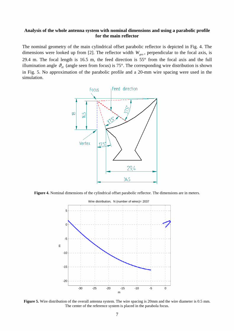
Analysis of the whole antenna system with nominal dimensions and using a parabolic profile for the main reflector

The nominal geometry of the main cylindrical offset parabolic reflector is depicted in Fig. 4. The dimensions were looked up from [2]. The reflector width geoW , perpendicular to the focal axis, is

29.4 m. The focal length is 16.5 m, the feed direction is 55° from the focal axis and the full illumination angle illϑ (angle seen from focus) is 75°. The corresponding wire distribution is shown

in Fig. 5. No approximation of the parabolic profile and a 20-mm wire spacing were used in the simulation.

Figure 4. Nominal dimensions of the cylindrical offset parabolic reflector. The dimensions are in meters.

-30 -25 -20 -15 -10 -5 0

-20

-15

-10

-5

0

5


m

m

Figure 5. Wire distribution of the overall antenna system. The wire spacing is 20mm and the wire diameter is 0.5 mm.

The center of the reference system is placed in the parabola focus.

8

The illumination distribution (normalized incident field) along the main reflector has been computed and reported in Fig. 6. The left side of the abscissa corresponds to the furthest wires from the vertex of the parabola. The edge taper is -25 dB and -21 dB at the left and right side of the reflector depicted in Fig. 5, respectively.

0 200 400 600 800 1000 1200 1400 1600 1800-30

-25

-20

-15

-10

-5

0

wire number

dBIllumination Distribution

Figure 6. Illumination distribution (normalized incident field) along the wires of the main reflector. Wire number 1 is

located in the upper left corner of Fig. 5.

The radiation pattern is shown in Figs. 7 and 8. The secondary lobe level is below -30 dB for each direction owing to the high edge taper. The 0° and 180°directions correspond to the zenith and the ground, respectively, when the antenna is pointed toward the zenith direction. According to Fig. 5, the 90° and -90° correspond to the horizon in the northern and southern directions, respectively.

-150 -100 -50 0 50 100 150-50

-45

-40

-35

-30

-25

-20

-15

-10

-5

0

Deg

Rad

iatio

n P

atte

rn (

dB)


Figure 7. Radiation pattern (normalized directivity) of the whole antenna system (secondary pattern) in the H-plane.

θθ=0°

θ=90°

θ=180°

θ=−90°

9

-5 -4 -3 -2 -1 0 1 2 3 4 5-40

-35

-30

-25

-20

-15

-10

-5

0

Deg

Rad

iatio

n P

atte

rn (

dB)


Figure 8. Zoom of the radiation pattern (normalized directivity) of the whole antenna system in the H-plane.

The Full Half Power Beam Width (FHPBW) is 1.88° and the maximum directivity is 22.5 dB. The latter leads to an antenna width efficiency η =0.70. Finally, the comparison between primary and secondary radiation patterns in Figs. 9 and 10 show that the secondary lobes which do not belong to the back of the reflector are produced by the subreflector.

-150 -100 -50 0 50 100 150-70

-60

-50

-40

-30

-20

-10

0

Deg

dB

Primary and Secondary Radiation patterns

Primary pattern

Main Refl. Scattered FieldSecondary Pattern

Main Refl. Angular Position

Figure 9. Comparison between primary and secondary radiation patterns in the H-plane.

θθ=0°

θ=90°

θ=180°

θ=−90°

Back of the reflector

10

-40 dB -20 dB

0 dB

30

210

60

240

90 270

120

300

150

330

180

0

Primary pattern



Figure 10. Comparison between primary and secondary radiation patterns in the H-plane.

θθ=0°

θ=90°

θ=180°

θ=−90°

11

Analysis of the whole antenna system with the real wire profile

The real geometry of the whole antenna system has been looked up from [3], where measured data are stored. The subreflector real profile is compared to the nominal one (from [1]) in Fig. 11. It should be noted that a slight aperture reduction (about 50 mm) as well as a tilt angle (about 0.5°) are present in the measured profile.

-1.5 -1 -0.5 0 0.5 115.5

16

16.5

17

17.5

m

m

Measured wire distribution

SourceNominal wire distribution

Figure 11. Wire distribution of the subreflector. The real wire spacing is approximately 10 mm (20 mm) in the part that

is closer to (further from) the source.

0 5 10 15 20 25 30

0

5

10

15

20

m

m

Measured ProfileNominal Vertex (0,0) m

Nominal Focus (0,16.5) m

Best Fit Vertex ∆=(-110.3,44.8) mm

Best Fit Focus ∆=(-6.5,-156.6) mm

Best Fit Parabola ∆θ=-0.365 Deg, eRMS=6.5 mm, eMAX=24.3 mm

Figure 12. Wire distribution of the main reflector: measured profile and best fit parabola.

12

Fig. 12 shows the measured main reflector profile. The wires are arranged in a piecewise fashion with 35 segments. The spacing is 20 mm for the first 25 bars that are closer to the vertex and 30 mm for the others. The origin of the measurement coordinate system coincides with the nominal vertex of the parabola. Therefore the nominal focus position is (0,16.5) m. A least square approximation has been carried out. The resulting “best fit” parabola is depicted in Fig. 12 as well. As reported in the figure legend, a slight tilt angle of about -0.4° in the parabola axis is present. Moreover, the focus and vertex of the best fit parabola have different positions with respect to the nominal ones. The discrepancies between nominal and estimated positions for the focus and vertex might be due to either a shape error of the reflector or to the measurement uncertainties. In order to compute the EM characteristics of the real structure, a simulation has been carried out. The results of the latter and the nominal case ones (see previous section) are both reported in Fig. 13. It should be noted that the two diagrams are practically coincident at every angle but around the maximum, where the secondary lobes of the measured profile case are higher. This phenomenon is probably related to the piecewise approximation of the parabolic profile.

-150 -100 -50 0 50 100 150-50

-45

-40

-35

-30

-25

-20

-15

-10

-5

0

Deg

Rad

iatio

n P

atte

rn (

dB)


with measured profile

with nominal profile

Figure 13. Radiation pattern computed from the measured wire profile and from the nominal wire profile (H-plane).

The close match between the two radiation patterns in Fig. 13 demonstrates that both manufacturing and measuring uncertainties are not significant at this operative frequency (408 MHz). Therefore, every subsequent design study concerning this antenna will be carried out on the basis of the nominal dimensions of the structure.

θθ=0°

θ=90°

θ=180°

θ=−90°

13

Optimization of the subreflector @ 408 MHz

In order to enhance the overall antenna width efficiency η a design study has been carried out on the subreflector, only varying the aperture dimension. The optimized geometry is shown in Fig. 14. The angle between the two arms is the same as in nominal case, whereas the aperture is reduced of 74%. Hence, the subreflector length is reduced as well. If the phase center of the new structure (0.15 m from the aperture) is placed in the focus of the main reflector, with the same 55° direction, the illumination distribution shown in Fig. 15 and the radiation pattern reported in Fig. 16 and 17 can be obtained.

-1 -0.8 -0.6 -0.4 -0.2 0 0.2 0.4 0.6 0.8 1

0

0.5

1

1.5


m

m

source

phase center

Figure 14. Geometry of the optimized subreflector.

0 200 400 600 800 1000 1200 1400 1600 1800-15

-10

-5

0

wire number

dB

Illumination Distribution

Figure 15. Illumination distribution of the optimized subreflector.

14

Thanks to the lower edge taper, the antenna efficiency η is now approximately 0.85 and the FHPBW is 1.54°. In the nominal case, the same values were η =0.70 and FHPBW=1.88°, respectively. The secondary lobes that are far from the maximum do not exhibit any increase. The first ones instead raise up to -20 dB, as shown in Fig. 17. If only the aperture reduction had been performed, without refocusing the feed, a width efficiency η =0.8 would have been obtained.

-150 -100 -50 0 50 100 150-50

-45

-40

-35

-30

-25

-20

-15

-10

-5

0

Deg

Rad

iatio

n P

atte

rn (

dB)


with optimized feed

with nominal feed

Figure 16. Radiation pattern of the whole system (secondary radiation pattern) in the H-plane for the optimized and

nominal case.

-5 -4 -3 -2 -1 0 1 2 3 4 5-30

-25

-20

-15

-10

-5

0

Deg

Rad

iatio

n P

atte

rn (

dB)


with optimized feed

with nominal feed

Figure 17. Zoom of the radiation pattern in the H-plane for the optimized and nominal case.

θθ=0°

θ=90°

θ=180°

θ=−90°

15

-150 -100 -50 0 50 100 150-70

-60

-50

-40

-30

-20

-10

0

Deg

dB

Primary and Secondary Radiation patterns

Primary pattern



Figure 18. Primary and secondary radiation patterns in the H-plane for the optmized case.

-40 dB -20 dB

0 dB

30

210

60

240

90 270

120

300

150

330

180

0

Primary pattern



Figure 19. Primary and secondary radiation patterns in the H-plane for the optmized case.

Finally, the comparison between primary and secondary radiation patterns in Figs. 18 and 19 show that the secondary lobes which do not belong to either the back of the reflector or the maximum area are produced by the subreflector.

θθ=0°

θ=90°

θ=180°

θ=−90°

θθ=0°

θ=90°

θ=180°

θ=−90°

16

Conclusions The EM analysis reported in this document demonstrated the good characteristic of the Northern Cross E/W Arm at 408 MHz. Moreover, excellent match has been achieved between the simulations that were performed on the nominal and measured wire profiles. Therefore, every subsequent design study concerning this antenna will be carried out on the basis of the nominal dimensions of the structure. A possible efficiency enhancement from η =0.70 to η =0.85 has been demonstrated. It entails a reduction of the subreflector wires and a subsequent refocusing. Bibliography [1] Stephen N. La and L. James, “Analysis of the Bologna Cross Radio Telescope”, CSIRO Division of Radiophysics, 5 April 1990 [2] Drawing K 52/9abcd, “Centine per Radiotelescopio” SAE S.p.A. Milano, Università di Bologna, Istituto di Fisica, 20 Febbraio 1962 [3] pUNTI e-w.xls, 26 Ottobre 2006

Microsoft Excel

Worksheet

17

Technical Report

Upgrade of the Northern Cross E/W Arm

for the 120÷240 MHz frequency band: general investigation and fat dipole solution

(Draft 1-EA/070410)


IEIIT-CNR




Torino 10th April 2007

18

This document contains a general investigation for the 120÷240 MHz frequency band upgrade of the Medicina Northern Cross E/W arm. As described in [1], the E/W arm of the Northern Cross is a cylindrical offset parabolic reflector with a feeding structure made up with a linear dipole array placed in a wire subreflector. The current antenna working frequency is 408 MHz, corresponding to a wavelength of 0.735 m. At this frequency, the aperture of the present subreflector (1.690 m) is larger than two wavelengths providing a high edge tapering (more than 20 dB) on the main cylindrical reflector. A new feed system working in the 120÷240 MHz frequency bandwidth has been studied with the same dipole and wire subreflector configuration. This structure is used to show the concepts and the critical aspects of a broadband reflector feed design as well as to demonstrate the incompatibility of the 120÷240 MHz working condition with the present subreflector dimensions. As a matter of fact, the wavelength that corresponds to the lower end of the 120÷240 MHz band is 2.5 m. In this case, a scaled version of the present subreflector would have a 5.75 m aperture. This value is obviously critical from the structural and manufacturing points of view. Moreover, it would also provide a 20 dB edge tapering which is not the optimum condition in terms of the overall antenna efficiency. In this work, the subreflector aperture is instead selected to obtain a minimum size structure which still provides a 5–8 dB edge tapering on the main reflector. However, the resulting value of 3 m is still far larger than the present 1.69 m. The design of antenna arrays with broadband operative conditions in both radiation pattern and impedance is not trivial. Both these features are required in order to feed a reflector with high efficiency in the overall frequency bandwidth. Owing to its complexity, the design problem has been attacked from different perspectives. A starting design was carried out with the 2-D analysis method described in [1]. The subreflector dimensions were determined to provide a proper edge tapering in the overall frequency bandwidth and according to reasonable dimensional constraints. The obtained geometry and the corresponding H-plane radiation patterns are reported in section 1. Subsequently, a 3-D method was used to design the linear array of radiators inside the subreflector. Single radiator dimensions as well as element spacing and optimum placement in the subreflector were obtained. The frequency behavior of the relevant quantities such as reflection coefficients, mutual couplings, feed tapering and the corresponding radiation patterns are reported in section 2. Finally, the radiation pattern of the whole antenna system, composed of the presented feed system and the main cylindrical reflector, are reported in section 3.

19

1. 120÷240 MHz Wire Subreflector Design The Pocklington’s equation 2-D method [1] has been used in this first design stage to define the subreflector dimensions according to the H-plane primary radiation pattern requirements i.e. proper edge tapering of the main reflector in the 120-240 MHz frequency bandwidth. The wire distribution of the designed subreflector is reported in Fig. 1. The red mark represents the position of the linear dipole array (modeled as a line source in this case). The corresponding H-plane radiation patterns at 120, 180 and 240 MHz are reported in Fig. 2. When the feed system is arranged as in Fig. 3 (see also [1]), the black dash-dot line of Fig. 2 at 37.5° corresponds to the angular position of the reflector edges in the feed polar coordinate system. As one can see from Fig. 2, the level of the feed system radiation pattern at 37.5° is -6 dB @ 120 MHz. Since the spatial attenuation at the left and right reflector edges of Fig. 3 (normalized to the center) is approximately 2 dB and -1 dB, respectively, the illumination distribution reported in Fig. 4 shows edge tapering levels of 8 dB and 5 dB. It should be remembered that the illumination distribution is the incident field along the main reflector wires. Even if a slightly higher edge taper could be desirable from the efficiency point of view, the present aperture choice w=3 m (1.2 λ1, where λ1=2.5 m) leads to reasonable dimensions of the feed system.

-1 -0.5 0 0.5 1

0

0.5

1

1.5

2

m

m

Figure 20. 2D geometry of the wire subreflector. The linear array position (line source) is represented with the red mark. The aperture size w is 3 m, the total length b is 2.25 m, the size of the back side A is 1.25 m and the distance d of the dipole array from the back of the subreflector is 0.5 m. The wire spacing of 20 mm leads to a 304 wire distribution. The wire diameter is 0.5 mm.

w

b

A

d

20

0 20 40 60 80 100 120 140 160 180-40

-35

-30

-25

-20

-15

-10

-5

0

Deg

dB

H-plane Primary Radiation Pattern

120 MHz

180 MHz240 MHz

Figure 21.Primary radiation patterns in the H-plane computed with the Pocklington’s equation method. The black dash-dot line at 37.5 ° represents the main reflector edges when the feed system is pointed as in Fig .3.

Figure 22. Feed system placement and relevant dimensions of the cylindrical offset parabolic reflector [1].

21

0 200 400 600 800 1000 1200 1400 1600 1800-15

-10

-5

0

Wire Number

dB

Illumination distribution along the main reflector wires

120 MHz

180 MHz

240 MHz

Figure 23. Illumination distribution (normalized incident field) along the main reflector wires. Wire number 1 is the furthest one from the vertex of the main parabolic cylindrical reflector (left side of Fig. 3). The feed system is pointed as in Fig. 3.

Another important feature is the frequency behavior of the radiation pattern. As can be noted from Fig. 2, it becomes narrower at higher frequencies (as expected). However, this narrowing effect is controlled so that the corresponding edge taper (Fig. 4) maintains proper 11–15 dB values even at the upper end of the bandwidth. This phenomenon is highlighted in Fig. 5, where the H-plane radiation pattern value at 37.5° versus frequency is reported. This quantity shows a minimum level of -13 dB at 220 MHz, corresponding to a maximum edge taper of 15 dB. The particular frequency behavior of Fig. 5 has been obtained by properly selecting the other three feed system dimensions (see Fig. 1). Roughly speaking, the feed system length b=2.25 m (0.9 λ1) was chosen to provide a proper quadratic phase error on the feed system aperture at higher frequencies. The choice of d= λ1/5 and A= λ1/2, besides providing a good matching behavior for the fat dipole array (see section 2), leads to a high radiation efficiency of the line source inside the subreflector at 120 MHz, but to a lower one at higher frequencies. This phenomenon produces aperture quadratic phase errors as well. Both these effects broaden the H-plane radiation pattern with respect to a non-quadratic-phased aperture. It should be noted that these phenomena have been exploited without significant distortions of the pattern such as split lobes, etc. (see Fig. 2). From Fig.2, secondary lobe levels and back radiation levels of the order of -25 dB and -30 dB, respectively, can be also estimated. Finally, the distance of the computed feed system phase center [1] from the aperture is reported in Fig. 6 as a function of frequency. The variation is not very large and, as can be noted in section 3, it does not produce any relevant defocusing loss on the whole antenna efficiency.

22

0.12 0.14 0.16 0.18 0.2 0.22 0.24-14

-13

-12

-11

-10

-9

-8

-7

-6

-5

GHz

dB

Feed Tapering at 37.5°

Figure 24. Value of the Primary Radiation pattern at 37.5° in the H-plane vs frequency.

0.12 0.14 0.16 0.18 0.2 0.22 0.24100

200

300

400

500

600

700

GHz

mm

Phase center

Figure 25. Distance of the computed phase center [1] from the aperture vs frequency.

23

2. Design of the Fat Dipole Linear array inside the Wire Subreflector A fat dipole linear array has been designed inside the subreflector of section 1, in order to provide a minimum complexity feed system solution. The radiator design as well as their optimum placement inside the wire subreflector has been carried out using a 3D EM simulator. Seven elements of the designed array configuration are shown in Fig. 7. Larger finite structures were also extensively simulated finding out that the relevant electromagnetic parameters can be already extrapolated from this 7-element array. For the sake of simulation simplicity, the subreflector wire distribution was substituted with a continuous PEC surface. Obviously, the agreement with the wire configuration has been verified. The fat dipoles were simulated as solid cylinders but, owing to their size, they can be built with metal pipes. The dipole length L = 0.42λ1 = 1.05 m, the diameter is 0.1L=105 mm, the source gap (gap between the two dipole arms) is 0.03λ1 =75 mm.

Figure 26. Seven fat dipole array inside the subreflector with discrete excitation ports.

The period of the structure is λ1/2=1.25 m. This value is a compromise between the mutual coupling at the lower frequencies and the grating lobes at the higher frequencies. Mutual couplings and reflection coefficients at 120, 180 and 240 MHz i.e. the diagonal and off-diagonal terms of the array scattering matrix are reported in Figs. 8, 9, 10, respectively. The performances of both central and edge elements can be seen in these figures. The reflection coefficient at 120 MHz (Fig. 8) is about -9 dB for the central elements 3, 4 and 5. This quantity increases for the edge elements owing to the truncation effect of both the array and subreflector. The mutual coupling between adjacent elements is -10 dB for the central elements and slightly higher for the edge ones. The coupling between non-adjacent elements is of the order of -17 dB. Thanks to this, the central elements 3, 4 and 5 are so slightly affected by the truncation effect that their behavior is independent of the array size. In other words, the data computed for these elements are still valid for larger arrays.

1 2 3 4 5 6 7

1 2 3 4 5 6 7

24

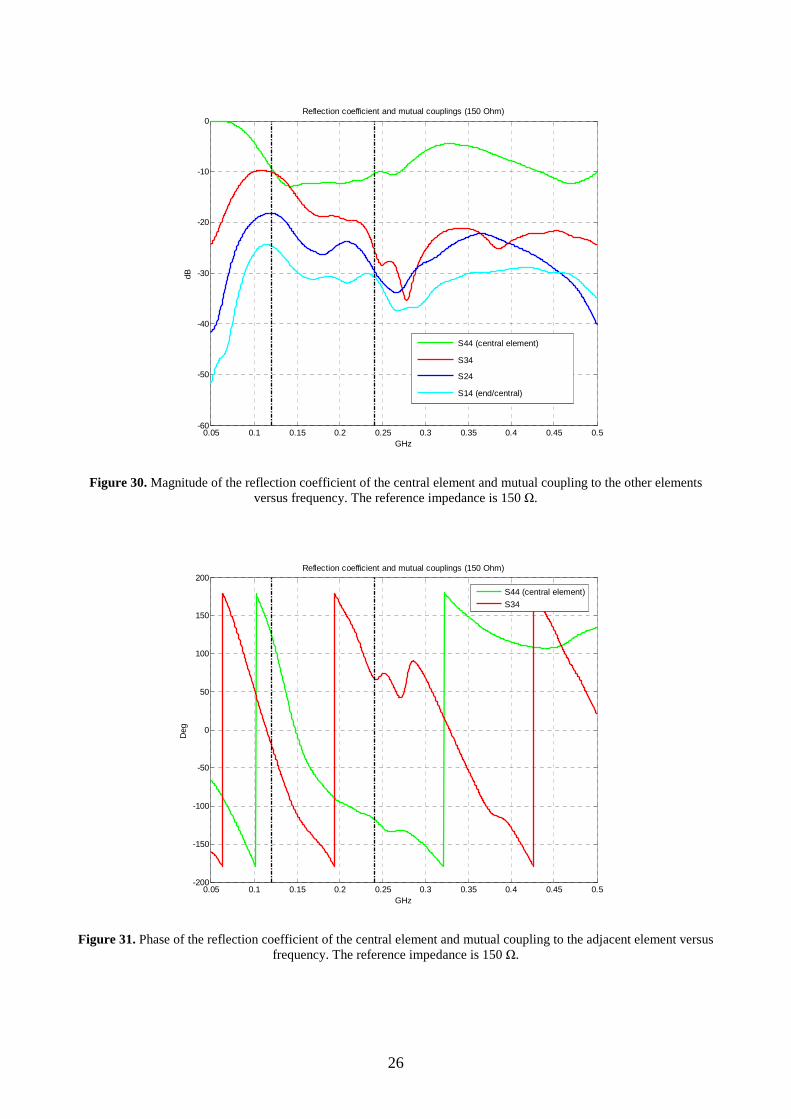
Analogous considerations apply for the higher frequencies (see Fig. 9 and 10). However, since the mutual coupling between adjacent elements quickly decreases with frequency (it is -19 dB and -26 dB at 180 MHz and 240 MHz, respectively), the truncation effect is less significant. Reflection coefficient of the central element as well as mutual coupling versus frequency is reported in Fig. 11. The reflection level is lower than -9 dB in the operative bandwidth. The mutual couplings are below -10 dB for frequencies above 120 MHz. The phase of the reflection coefficient and the adjacent element mutual coupling is shown in Fig. 12. As can be observed, these terms are nearly counter-phased in the overall frequency bandwidth.

1 2 3 4 5 6 7-50

-45

-40

-35

-30

-25

-20

-15

-10

-5

Radiator Number n

dB

Reflection Coefficients and Mutual Couplings @ 120 MHz

S1n

S2n

S3n

S4n

S5n

S6n

S7n

Figure 27. Reflection coefficients and mutual couplings for the 7 dipole array of Fig. 7 @ 120 MHz. The reference

impedance is 150 Ω.

25

1 2 3 4 5 6 7-50

-45

-40

-35

-30

-25

-20

-15

-10

-5

Radiator Number n

dB


S1n

S2n

S3n

S4n

S5n

S6n

S7n



1 2 3 4 5 6 7-50

-45

-40

-35

-30

-25

-20

-15

-10

-5

Radiator Number n

dB


S1n

S2n

S3n

S4n

S5n

S6n

S7n



26

0.05 0.1 0.15 0.2 0.25 0.3 0.35 0.4 0.45 0.5-60

-50

-40

-30

-20

-10

0

GHz

dB

Reflection coefficient and mutual couplings (150 Ohm)

S44 (central element)

S34

S24

S14 (end/central)

Figure 30. Magnitude of the reflection coefficient of the central element and mutual coupling to the other elements

versus frequency. The reference impedance is 150 Ω.

0.05 0.1 0.15 0.2 0.25 0.3 0.35 0.4 0.45 0.5-200

-150

-100

-50

0

50

100

150

200

GHz

Deg

Reflection coefficient and mutual couplings (150 Ohm)

S44 (central element)

S34

Figure 31. Phase of the reflection coefficient of the central element and mutual coupling to the adjacent element versus

frequency. The reference impedance is 150 Ω.

27

The previous characterization of the finite array is based on single element excitation. However, another way of studying antenna arrays is the infinite array approach. In this case, the unit cell of the periodic structure (i.e. infinite array) is analyzed for different incidence angles. The reflection coefficient of the unit cell for broadside incidence is reported in Fig. 13 in comparison with the reflection coefficient of the central element of the finite array. As expected, these quantities differ from each other because they refer to two different working conditions. From the receiver design point of view, the first can be interpreted as the reflection coefficient at the input port of a corporate beam forming network (for broadside operation) connected to the array. The second is instead the reflection coefficient at the input port of one of the array elements. Hence, the second parameter should be considered for the digital beam forming network receiver design.

0.05 0.1 0.15 0.2 0.25 0.3 0.35 0.4 0.45 0.5-20

-18

-16

-14

-12

-10

-8

-6

-4

-2

0

GHz

dB

Reflection coefficient (150 Ohm)

Infinite array (broadside)

7 element array (central element)

Figure 32. Reflection coefficient of the infinite array unit cell and for single excitation in the 7-element array. The

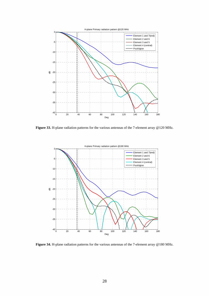
reference impedance is 150 Ω. The radiation pattern for each array element has also been computed. The H-plane cuts at 120, 180 and 240 MHz are shown in Figs. 14, 15 and 16, respectively. The H-plane patterns computed with the Pocklington method (same as Fig. 2) are reported in the corresponding figures for comparison. The discrepancies between the various patterns are due to the diffracted field arising from the edges of the array. Nevertheless, apart from the edge elements, the various patterns are still consistent with the Pocklington simulation in terms of feed system tapering at 37.5°, profile of the secondary lobes and front-to-back ratio. Therefore, the designed structure can be used to efficiently feed the main reflector.

28

0 20 40 60 80 100 120 140 160 180-40

-35

-30

-25

-20

-15

-10

-5

0

Deg

dB

H-plane Primary radiation pattern @120 MHz

Element 1 and 7(end)

Element 2 and 6

Element 3 and 5Element 4 (central)

Pockligton

Figure 33. H-plane radiation patterns for the various antennas of the 7-element array @120 MHz.

0 20 40 60 80 100 120 140 160 180-40

-35

-30

-25

-20

-15

-10

-5

0

Deg

dB



Element 2 and 6


Pockligton

Figure 34. H-plane radiation patterns for the various antennas of the 7-element array @180 MHz.

29

0 20 40 60 80 100 120 140 160 180-40

-35

-30

-25

-20

-15

-10

-5

0

Deg

dB



Element 2 and 6


Pockligton

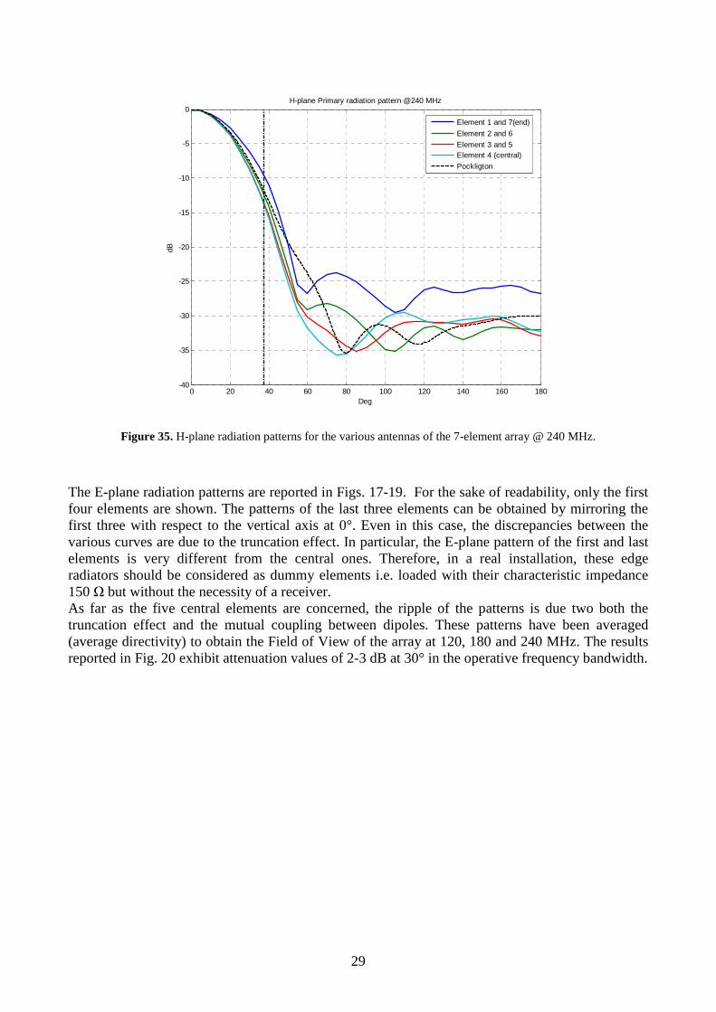
Figure 35. H-plane radiation patterns for the various antennas of the 7-element array @ 240 MHz.

The E-plane radiation patterns are reported in Figs. 17-19. For the sake of readability, only the first four elements are shown. The patterns of the last three elements can be obtained by mirroring the first three with respect to the vertical axis at 0°. Even in this case, the discrepancies between the various curves are due to the truncation effect. In particular, the E-plane pattern of the first and last elements is very different from the central ones. Therefore, in a real installation, these edge radiators should be considered as dummy elements i.e. loaded with their characteristic impedance 150 Ω but without the necessity of a receiver. As far as the five central elements are concerned, the ripple of the patterns is due two both the truncation effect and the mutual coupling between dipoles. These patterns have been averaged (average directivity) to obtain the Field of View of the array at 120, 180 and 240 MHz. The results reported in Fig. 20 exhibit attenuation values of 2-3 dB at 30° in the operative frequency bandwidth.

30

-150 -100 -50 0 50 100 150-40

-35

-30

-25

-20

-15

-10

-5

0

Deg

dB

E-plane Primary radiation pattern @120 MHz

Element 1 (end)

Element 2

Element 3

Element 4 (central)

Figure 36. E-plane radiation patterns for the various antennas of the 7-element array @ 120 MHz.

-150 -100 -50 0 50 100 150-40

-35

-30

-25

-20

-15

-10

-5

0

Deg

dB


Element 1 (end)

Element 2

Element 3

Element 4 (central)


31

-150 -100 -50 0 50 100 150-40

-35

-30

-25

-20

-15

-10

-5

0

Deg

dB


Element 1 (end)

Element 2

Element 3

Element 4 (central)


-150 -100 -50 0 50 100 150-40

-35

-30

-25

-20

-15

-10

-5

0

Deg

dB

E-plane Mean Primary radiation pattern

120 MHz

180 MHz240 MHz

Figure 39. Field of view of the array element. The values at 30° (red dash-dotted line) are -1.9, -2.2 and -3.1 dB at 120,

180 and 240 MHz, respectively.

32

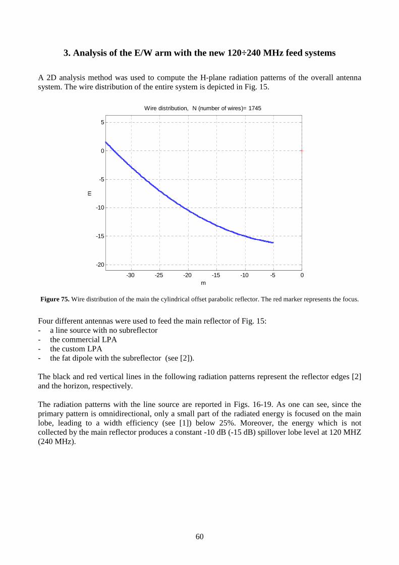
3. Analysis of the E/W arm with the new 120÷240 MHz feed system

The 2D analysis method was used to compute the H-plane radiation patterns of the overall antenna system. Since the H-plane radiation patterns of the single array element (see Fig. 14-16) computed with the 3D method were consistent with the 2D ones, the latter were used for the final analysis. In this way, even the interaction between the sub and main reflectors has been taken into account. The wire distribution of the entire system is depicted in Fig. 21. The feed system direction is 55° from the focal axis as in Fig. 3. The phase center of the feed system at lower frequencies (0.2 m far from the aperture) is placed in the focus of the parabolic reflector.

-30 -25 -20 -15 -10 -5 0

-20

-15

-10

-5

0

5


m

m

Figure 40. Wire distribution of the antenna system with the feed system (upper right corner) and main the cylindrical

offset parabolic reflector. The computed H-plane patterns are shown in Figs. 22-27. The blue line refers to the whole antenna system (secondary pattern), the red line is the feed system pattern (primary pattern) and the green one is the main reflector scattered field. Since the feed system pattern is computed in presence of the main reflector, the interaction leads to a non symmetric primary pattern with respect to feed system pointing direction. Owing to the low edge tapering at 120 MHz (see Fig. 4), the secondary lobes and the spillover lobes in Figs. 22 and 23 are approximately -17 dB. These quantities are instead below -26 dB at higher frequencies.

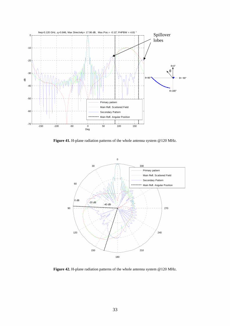
33

-150 -100 -50 0 50 100 150-70

-60

-50

-40

-30

-20

-10

0

Deg

dB

freq=0.120 GHz, η=0.846, Max Directivity= 17.96 dB, Max.Pos.= -0.12°, FHPBW = 4.81 °

Primary pattern

Main Refl. Scattered Field

Secondary Pattern


Figure 41. H-plane radiation patterns of the whole antenna system @120 MHz.

-40 dB -20 dB

0 dB

30

210

60

240

90 270

120

300

150

330

180

0

Primary pattern


Secondary Pattern



θθ=0°

θ=90°

θ=180°

θ=−90°

Spillover lobes

34

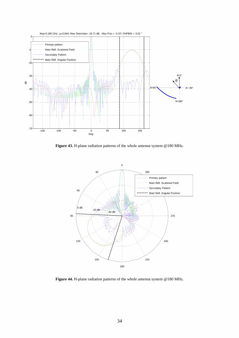
-150 -100 -50 0 50 100 150-70

-60

-50

-40

-30

-20

-10

0

Deg

dB


Primary pattern


Secondary Pattern



-40 dB -20 dB

0 dB

30

210

60

240

90 270

120

300

150

330

180

0

Primary pattern


Secondary Pattern



θθ=0°

θ=90°

θ=180°

θ=−90°

35

-150 -100 -50 0 50 100 150-70

-60

-50

-40

-30

-20

-10

0

Deg

dB


Primary pattern


Secondary Pattern



-40 dB -20 dB

0 dB

30

210

60

240

90 270

120

300

150

330

180

0Primary pattern


Secondary Pattern



The other antenna parameters such as directivity (see [1]), Full Half Power Beam Width (FHPBW) and efficiency are reported in Figs. 28-30 as a function of frequency. As one can see, no gap in the frequency behavior is present providing a real broadband operation condition. The ripple of the various curves is due to the interaction between sub and main reflectors.

θθ=0°

θ=90°

θ=180°

θ=−90°

36

Since the efficiency (reported in Fig. 3) is good in the whole bandwidth (η> 0.8), the directivity at the upper frequencies (21 dB) is 3 dB higher than at the lower ones (18 dB). The FHPBW (Fig. 29) is approximately 4.8° and 2.6° at 120 and 240 MHz, respectively. The curve of the antenna efficiency reported in Fig. 30 is related to the frequency behavior of the feed system tapering in Fig. 5. At the lower end of the bandwidth, the efficiency increases with frequency because the feed system directivity increases, reducing the spillover losses. The minimum at 220 MHz corresponds to the maximum feed system tapering of Fig. 5.

0.12 0.14 0.16 0.18 0.2 0.22 0.2417.5

18

18.5

19

19.5

20

20.5

21

GHz

dB

Antenna Gain

Figure 47. Directivity [1] of the complete antenna system.

Directivity

37

0.12 0.14 0.16 0.18 0.2 0.22 0.242.5

3

3.5

4

4.5

5

GHz

Deg

FHPBW

Figure 48. Full Half-Power Beam Width of the complete antenna system.

0.12 0.14 0.16 0.18 0.2 0.22 0.2480

81

82

83

84

85

86

87

88

GHz

%

Aperture Efficiency

Figure 49. Efficiency of the complete antenna system.

38

Conclusions A preliminary upgrade study for the illumination of the Northern Cross E/W arm in the 120÷240 MHz frequency band has been presented. It showed good performances with a minimum complexity structure. In the whole frequency bandwidth, the overall antenna efficiency in the H-plane is better than 0.8, the H-plane HPBW decrease from 4.8° to 2.6°, the E-plane Field of View is about ± 30° for pattern attenuation lower than 3 dB, the reflection coefficient is better than -9 dB when a 150 Ω impedance is used. Mutual coupling between the array elements has also been estimated providing a -10 dB upper bound. Thanks to this value, only two dummy elements are needed in the final array configuration. Other radiator geometries will be presented in the following reports.

References

[1] G. Virone, R. Tascone, O. A. Peverini, G. Addamo, A. Olivieri, “EM Analysis of the Northern Cross E/W Arm @ 408 MHz” IEIIT Technical Report EA061103

39

Technical Report


for the 120÷240 MHz frequency band: dense array solution

(Draft 1-EA/070426)


IEIIT-CNR




Torino 26th April 2007

40

A preliminary solution for the 120÷240 MHz upgrade of the Northern Cross E/W arm has been proposed in [1]. In such design study, fat dipoles were arranged in a sparse array configuration i.e. the inter-element spacing of the radiators was larger than half wavelength at the highest working frequency [2]. It was in fact half wavelength at the lowest frequency (λ1/2=1.25 m). Hence, grating lobes occur with that configuration at the higher frequencies, when the array beam is scanned away from broadside. A dense array configuration is instead investigated in the present document. It is based on a branched Vivaldi linear array arranged inside a subreflector. The inter-element spacing is λ1/4.5 = 0.556 m providing a grating-lobe free 120÷240 MHz frequency bandwidth for each scanning angle. Moreover, the designed array also operates in the present bandwidth of the Medicina Radiotelescope [3] centered at 408 MHz. The λ1/4.5 inter-element spacing guarantees a grating-lobe free condition at broadside up to 430 MHz and more. The 3D view of the proposed solution is reported in Fig. 1. As one can see, the branched Vivaldi radiators are connected to each other. Moreover, they are also directly connected to the subreflector through a metal plate. Circular stubs are drilled on this plate to create wideband open circuits. The excitation is provided at the junction between the circular stub and the tapered slotline section of each Vivaldi radiator. Thanks to the circular stub, even an unbalanced (coaxial cable) excitation can be directly connected to the radiators. The subreflector is simulated as a PEC surface. Its dimensions are reported in the side view of Fig. 2.

Figure 50. Linear array of branched Vivaldi radiators inside the subreflector.

Subreflector

Metal plate with circular stubs Branched

Vivaldi radiators

Excitation Tapered slotline

41

Figure 51. Side view of the branched Vivaldi linear array inside the subreflector. The aperture W is equal to 1.2 λ1 = 3 m (as in [1]), the length of the subreflector section Lsub is equal to 1 λ1 = 2.5 m, the radiator length Lrad is equal to 0.82 λ1

= 2.05 m. The transition section is A= λ1/4.5=0.556 m wide and Lback= λ1/6=0.417 m long. The width of the radiator branches s is 0.02 λ1 = 50 mm.

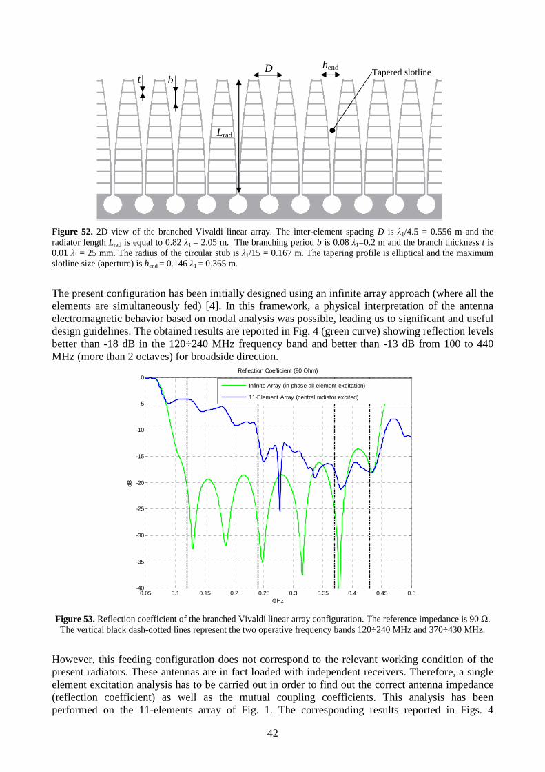
Such subreflector dimensions are comparable to the ones reported in [1]. It should be noted that the length of the radiators Lrad= 0.82 λ1 = 2.05 m is less than the subreflector one Lsub= λ1 = 2.5 m. The lower part of Fig. 2 shows the transition section wherein the circular stubs are placed. The slotline tapering starts at the interface between the transition and the subreflector sections. The other relevant dimensions are reported in Fig. 3 where only the radiators are shown. The inter-element spacing D is equal to λ1/4.5 = 0.556 m. The branching period b is 0.08 λ1=0.2 m and the branch thickness t is 0.01 λ1 = 25 mm. All the various branches can be manufactured with metal bars having a 50x25 mm2 section. It should be noted that these quantities could be modified in order to meet industrial standards for a possible final low-cost manufacturing-oriented design.

W

Lsub

Lback

A

Lrad

s

42

Figure 52. 2D view of the branched Vivaldi linear array. The inter-element spacing D is λ1/4.5 = 0.556 m and the radiator length Lrad is equal to 0.82 λ1 = 2.05 m. The branching period b is 0.08 λ1=0.2 m and the branch thickness t is 0.01 λ1 = 25 mm. The radius of the circular stub is λ1/15 = 0.167 m. The tapering profile is elliptical and the maximum slotline size (aperture) is hend = 0.146 λ1 = 0.365 m.

The present configuration has been initially designed using an infinite array approach (where all the elements are simultaneously fed) [4]. In this framework, a physical interpretation of the antenna electromagnetic behavior based on modal analysis was possible, leading us to significant and useful design guidelines. The obtained results are reported in Fig. 4 (green curve) showing reflection levels better than -18 dB in the 120÷240 MHz frequency band and better than -13 dB from 100 to 440 MHz (more than 2 octaves) for broadside direction.

0.05 0.1 0.15 0.2 0.25 0.3 0.35 0.4 0.45 0.5-40

-35

-30

-25

-20

-15

-10

-5

0

GHz

dB

Reflection Coefficient (90 Ohm)

Infinite Array (in-phase all-element excitation)

11-Element Array (central radiator excited)

Figure 53. Reflection coefficient of the branched Vivaldi linear array configuration. The reference impedance is 90 Ω. The vertical black dash-dotted lines represent the two operative frequency bands 120÷240 MHz and 370÷430 MHz.

However, this feeding configuration does not correspond to the relevant working condition of the present radiators. These antennas are in fact loaded with independent receivers. Therefore, a single element excitation analysis has to be carried out in order to find out the correct antenna impedance (reflection coefficient) as well as the mutual coupling coefficients. This analysis has been performed on the 11-elements array of Fig. 1. The corresponding results reported in Figs. 4

Lrad

D hend Tapered slotline

b t

43

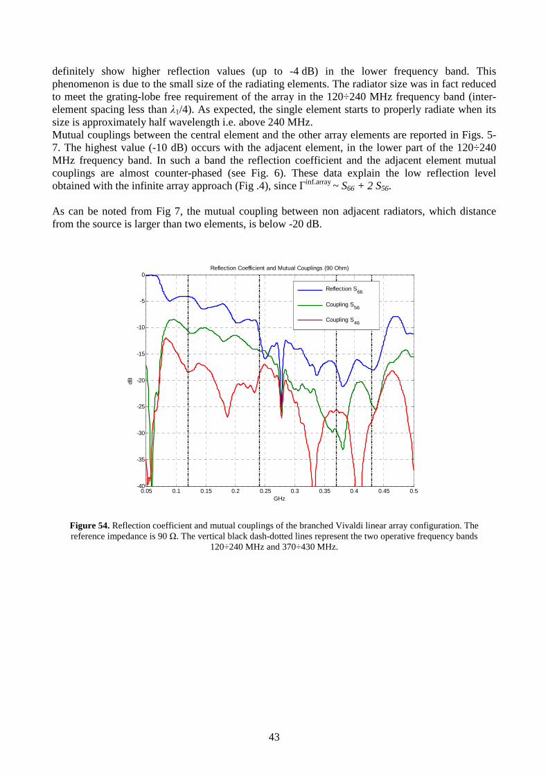
definitely show higher reflection values (up to -4 dB) in the lower frequency band. This phenomenon is due to the small size of the radiating elements. The radiator size was in fact reduced to meet the grating-lobe free requirement of the array in the 120÷240 MHz frequency band (inter-element spacing less than λ1/4). As expected, the single element starts to properly radiate when its size is approximately half wavelength i.e. above 240 MHz. Mutual couplings between the central element and the other array elements are reported in Figs. 5-7. The highest value (-10 dB) occurs with the adjacent element, in the lower part of the 120÷240 MHz frequency band. In such a band the reflection coefficient and the adjacent element mutual couplings are almost counter-phased (see Fig. 6). These data explain the low reflection level obtained with the infinite array approach (Fig .4), since Γinf.array ~ S66 + 2 S56. As can be noted from Fig 7, the mutual coupling between non adjacent radiators, which distance from the source is larger than two elements, is below -20 dB.

0.05 0.1 0.15 0.2 0.25 0.3 0.35 0.4 0.45 0.5-40

-35

-30

-25

-20

-15

-10

-5

0

GHz

dB

Reflection Coefficient and Mutual Couplings (90 Ohm)

Reflection S66

Coupling S56

Coupling S46

Figure 54. Reflection coefficient and mutual couplings of the branched Vivaldi linear array configuration. The reference impedance is 90 Ω. The vertical black dash-dotted lines represent the two operative frequency bands

120÷240 MHz and 370÷430 MHz.

44

0.05 0.1 0.15 0.2 0.25 0.3 0.35 0.4 0.45 0.5-200

-150

-100

-50

0

50

100

150

200

GHz

Deg

Phase of the mutual coupling ratio S56/S66

Figure 55. Phase difference between reflection coefficient and mutual coupling to the adjacent element for the central

branched Vivaldi radiator in the 11-element array.

0.05 0.1 0.15 0.2 0.25 0.3 0.35 0.4 0.45 0.5-40

-35

-30

-25

-20

-15

-10

-5

0

GHz

dB

Reflection Coefficient and Mutual Couplings (90 Ohm)

Reflection S66

Coupling S36

Coupling S26

Coupling S16

Figure 56. Reflection coefficient and mutual couplings of the branched Vivaldi linear array configuration. The reference impedance is 90 Ω. The vertical black dash-dotted lines represent the two operative frequency bands

120÷240 MHz and 370÷430 MHz.

Radiation patterns in the H-plane were computed with both the infinite (all-elements in-phase excitation) and finite (single element excitation) approaches. The obtained results at 120, 240 and 408 MHz are reported in Figs. 8, 9 and 10, respectively. The discrepancies between the two curves,

45

which should nominally be the same, are due to the array truncation. As expected, this effect is less significant at higher frequencies. Hence, the green curve should be considered to estimate the H-plane radiation pattern of the elements that are far from the edges in larger finite arrays. Since the H-plane patterns computed with the infinite array approach show a similar behavior with respect to the ones reported in [1] i.e. 37.5° tapering from -6 dB to -12 dB and a high front-to-back ratio, the present structure can feed the Northern Cross E/W cylindrical offset parabolic reflector with great efficiency in the continuous bandwidth from 120 to 430 MHz. E-plane radiation patterns at 120, 240 and 408 MHz of the 11-element array central element are shown in Fig. 11. The ripple of the curves is due to the great interaction among the elements and the array truncation. The vertical dash-dotted line at 30° represents the 3-dB field of view of the fat dipole configuration reported in [1]. As can be noted, the present configuration exhibits a narrower field of view (approximately 20°) with respect to the solution in [1]. As a matter of fact, the Vivaldi antenna in its relevant configuration presents a higher directivity because of the stronger aperture coupling with the adjacent elements.

0 20 40 60 80 100 120 140 160 180-40

-35

-30

-25

-20

-15

-10

-5

0

GHz

dB

H-plane Radiation Pattern @ 120 MHz



Figure 57. H-plane radiation pattern of the branched Vivaldi array inside the subreflector @ 120 MHz. The black dash-

dot line at 37.5 ° represents the main reflector edges when the feed system is pointed as in [1].

46

0 20 40 60 80 100 120 140 160 180-40

-35

-30

-25

-20

-15

-10

-5

0

GHz

dB






0 20 40 60 80 100 120 140 160 180-40

-35

-30

-25

-20

-15

-10

-5

0

GHz

dB






47

0 20 40 60 80 100 120 140 160 180-40

-35

-30

-25

-20

-15

-10

-5

0

GHz

dB

E-plane Radiation Pattern

120 MHz

240 MHz408 MHz

Figure 60. E-plane radiation patterns of the branched Vivaldi array inside the subreflector (single element excitation).

The black dash-dot line at 30 ° represents the Field of View of the fat dipole configuration reported in [1].

48

Conclusions

A dense array has been designed to feed the Northern Cross E/W arm main reflector. It is composed of branched Vivaldi radiators arranged inside a subreflector in a linear array configuration. This one is grating-lobe free for each scanning angle up to 240 MHz owing to the close spacing of the elements. It is also grating-lobe free at broadside up to 430 MHz and more. However, such close spacing implies reduced dimensions of the radiating elements, leading to a high reflection coefficient (up to -4 dB) at 120 MHz. Moreover, a strong array truncation effect has been observed at 120 MHz for radiation pattern in both E- and H-planes. Therefore, more than one dummy element should be used at the array edges in order not to have great discrepancies among the various element patterns. Finally, it was observed that the E-plane field of view of this configuration is narrower with respect to the fat dipole one [1] owing to the own directivity of the Vivaldi-type radiators in their working condition.

References

[2] G. Virone, R. Tascone, O. A. Peverini, G. Addamo, A. Olivieri, “Upgrade of the Northern

Cross E/W Arm for the 120÷240 MHz frequency band: preliminary investigation” IEIIT Technical Report EA070410

[3] W.A. van Cappellen, S.J. Wijnholds, J. D. Bregman, “Sparse antenna array configurations in large aperture synthesis radio telescopes”, Proceedings of the 3rd European Radar Conference, Manchester UK, September 2006, pp. 76-79

[4] G. Virone, R. Tascone, O. A. Peverini, G. Addamo, A. Olivieri, “EM Analysis of the Northern Cross E/W Arm @ 408 MHz” IEIIT Technical Report EA061103

[5] J. Shin and D. H. Schaubert, “A Parameter Study of Stripline-Fed Vivaldi Notch-Antenna Arrays”, IEEE Transactions on Antenna and Propagation, Vol. 47, No. 5, May 1999, pp. 879-886

49

Technical Report


for the 120÷240 MHz frequency band: log periodic antenna solution

(Draft 1-EA/070719)


IEIIT-CNR




Torino 19th July 2007

50

This document contains a further investigation for the 120÷240 MHz upgrade of the Medicina Northern Cross E/W arm [1]. The fat dipole and the branched Vivaldi solutions were presented in [2] and [3], respectively. Both these configurations make use of a wire subreflector to achieve the directivity required to feed the main reflector. In this way, high illumination efficiency and large field of view were obtained with low spillover losses. However, the presence of the wire subreflector leads to an increased mechanical complexity, weight and cost of the feed system which is not suitable for a first low-frequency test-bed. For this reason, a subreflectorless solution is presented in this work. It consists of an array of log periodic antennas (LPAs) placed in the focus of the main reflector. This solution was previously discarded by the IEIIT group since a radiation pattern which is broad in the E-plane (large field-of-view) and narrower in the H-plane (proper illumination of the main reflector) is needed in the present application. On the contrary, the LPA has instead a radiation pattern which is narrower in the E-plane than in the H-plane. Therefore, reduced performances should be expected with this configuration. In order to further reduce the costs, a commercial LPA has been initially selected. The computed reflection coefficient and radiation patterns for this antenna are reported in section 1. However, since the previous antenna is not the optimum LPA for the present application, another LPA has been designed in order to show the achievable performances of this subreflectorless solution. The corresponding simulated parameters are reported in section 2. Finally, the radiation pattern of the whole antenna system with the LPAs is reported in section 3. The comparison to the fat dipole solution (with subreflector) is also shown in order to quantify the pattern and efficiency degradations.

51

1. Commercial LPA 100÷500 MHz, 1.2 m, 18 elements

The LPA reported in Fig. 1 is a commercial model. Its operative frequency band is 100÷500 MHz and the typical gain is 6 dB. This antenna has been simulated in order to verify the nominal data and to obtain the radiation patterns at 120 and 240 MHz.

Figure 61. Commercial LPA with 18 elements, total length 1.2 m, longer dipole length 1.505 m, shorter dipole length

0.215 m.

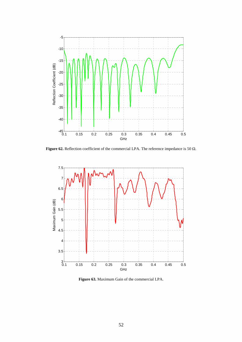
The reflection coefficient in the 100÷500 MHz band is reported in Fig. 2, confirming the 50-Ω impedance matching in the overall band. The antenna maximum gain is instead reported in Fig. 3. The level is even better than 6 dB but at some frequencies the gain drops to very low values. At those frequencies, the corresponding radiation patterns are very distorted. The radiation patterns in the H-plane and the E-plane are reported in Figs. 4 and 5, respectively. Thanks to the properties of the LPA and since this antenna is designed for a maximum working frequency of 500 MHz, the patterns at 120 MHz and 240 MHz are practically coincident. The H-plane pattern level at 37.5° (edge of the main reflector [2]) is approximately -1.1 dB leading to a poor tapering of the main reflector (see section 3). As expected, the E-plane pattern is narrower than the H-plane one and the front-to-back ratio is of the order of 20 dB.

52

0.1 0.15 0.2 0.25 0.3 0.35 0.4 0.45 0.5-45

-40

-35

-30

-25

-20

-15

-10

-5

GHz

Ref

lect

ion

Coe

ffic

ient

(dB

)

Figure 62. Reflection coefficient of the commercial LPA. The reference impedance is 50 Ω.

0.1 0.15 0.2 0.25 0.3 0.35 0.4 0.45 0.53

3.5

4

4.5

5

5.5

6

6.5

7

7.5

GHz

Max

imum

Gai

n (d

B)

Figure 63. Maximum Gain of the commercial LPA.

53

-150 -100 -50 0 50 100 150-40

-35

-30

-25

-20

-15

-10

-5

0

Deg

Rad

iatio

n P

atte

rn (

dB)

H-plane

120 MHz

240 MHz

Figure 64. H-plane Radiation Pattern of the commercial LPA. The black dash-dot lines at 37.5 ° and -37.5 ° represent the main reflector edges when the antenna is pointed at 55° with respect to the axis of the parabolic profile. The values

of the pattern at 37.5° are -1.1 dB at both frequencies.

-150 -100 -50 0 50 100 150-40

-35

-30

-25

-20

-15

-10

-5

0

Deg

Rad

iatio

n P

atte

rn (

dB)

E-plane

120 MHz

240 MHz

Figure 65. E-plane Radiation Pattern of the commercial LPA. The HPBW is approximately 70°.

54

2. Custom LPA 120÷240 MHz, 2.2 m, 18 elements

A new LPA has been designed in the 120÷240 MHz frequency band with a higher directivity with respect to the commercial one, in order to improve the main reflector illumination efficiency. The designed structure, which is shown in Fig. 6, has 18 elements and is 2.2 meters long. The estimated weight is 3.7 Kg.

Figure 66. Custom LPA with 18 elements, length 2.2 m, longer dipole length 1.275 m, shorter dipole length 0.49 m.

The reflection coefficient is reported in Fig. 7, showing a good 50-Ω impedance matching in a frequency band that is slightly larger than 120÷240 MHz. The maximum gain reported in Fig. 8 is about 9.5 dB at the lower end of the band, and smoothly decreases to 7.5 dB at the upper end, without significant ripple. Due to the different gain values at 120 MHz and 240 MHz, the H-plane radiation patterns in Fig. 9 are different: the pattern levels at 37.5° are in fact -2.7 dB and -1.8 dB, respectively. As it will be shown in section 3, this phenomenon is suitable for the present application because the narrower beamwidth at the lower frequencies provides a better tapering of the main reflector with a consequent reduction of the splillover lobes. Since the spillover lobes are nominally lower at the higher frequencies, this slightly broader beamwidth @240 MHz can be tolerated since it avoids an excessive LPA length and weight. Even in this case, the E-plane pattern is narrower than the H-plane one but it is quite constant with frequency. The front-to-back ratio is better than 20 dB.

55

0.1 0.15 0.2 0.25 0.3 0.35 0.4 0.45 0.5-50

-45

-40

-35

-30

-25

-20

-15

-10

-5

0

GHz

Ref

lect

ion

Coe

ffic

ient

(dB

)

Figure 67. Reflection coefficient of the custom LPA, the reference impedance is 50 Ω.

0.1 0.12 0.14 0.16 0.18 0.2 0.22 0.24 0.26 0.280

1

2

3

4

5

6

7

8

9

10

GHz

Max

imum

Gai

n (d

B)

Figure 68. Maximum gain of the custom LPA.

56

-150 -100 -50 0 50 100 150-40

-35

-30

-25

-20

-15

-10

-5

0

Deg

Rad

iatio

n P

atte

rn (

dB)

H-plane

120 MHz

240 MHz

Figure 69. H-plane Radiation Pattern of the custom LPA. The black dash-dot lines at 37.5 ° and - 37.5 ° represent the main reflector edges when the antenna is pointed at 55° with respect to the axis of the parabolic profile. The values of

the pattern at 37.5° are -2.7 dB and -1.8 dB at 120 MHz and 240 MHz, respectively.

-150 -100 -50 0 50 100 150-40

-35

-30

-25

-20

-15

-10

-5

0

Deg

Rad

iatio

n P

atte

rn (

dB)

E-plane

120 MHz

240 MHz

Figure 70. E-plane Radiation Pattern of the custom LPA. The HPBW is approximately 60°.

The custom LPA was also analyzed in a 7-element array configuration in order to compute the mutual couplings and estimate the field-of-view. The inter-element spacing was 1.25 m, as in [2] (sparse array). It has to be noted that this arrangement, where the inter-element spacing is slightly

57

smaller than the antenna maximum dimension (1.275 m) is possible due to the LPA geometry (the two arms of the dipoles are slightly displaced from the center of the LPA). The reflection coefficient of the central element of the array, reported in Fig. 11, does not show significant differences with respect to the single LPA case (Fig. 7). The mutual coupling between the central element and the neighbors is below -30 dB.

The maximum gain of the central element (shown in Fig. 12) is smaller than the one of the LPA alone (Fig. 8) in the lower part of the frequency band. This phenomenon is related to the coupling that broadens the E-plane pattern of the central element at lower frequencies. As reported in Fig. 13, the E-plane pattern at 120 MHz is in fact broader than the one of the single LPA (Fig. 10). On the contrary, the pattern at 240 MHz, where the coupling is less significant, remains almost the same as in the single LPA case. From Fig. 13, it has to be concluded that the field-of-view of the present feed system is comparable to the one of the fat dipole solution described in [2]. As far as the H-plane radiation pattern is concerned, only a slight narrowing effect is observed at 120 MHz.

0.1 0.15 0.2 0.25 0.3 0.35 0.4 0.45 0.5-60

-50

-40

-30

-20

-10

0

GHz

Ref

lect

ion

Coe

ffic

ient

(dB

)

S44 (central)

S43

S42

Figure 71. Reflection coefficient (S44) of the central radiator of the 7-element custom LPA array, and mutual couplings

(S43 and S42), the reference impedance is 50 Ω.

58

0.1 0.12 0.14 0.16 0.18 0.2 0.22 0.24 0.26 0.280

1

2

3

4

5

6

7

8

9

10

GHz

Max

imum

Gai

n (d

B)

Figure 72. Maximum gain of the central radiator of the 7-element custom LPA array.

-150 -100 -50 0 50 100 150-40

-35

-30

-25

-20

-15

-10

-5

0

Deg

Rad

iatio

n P

atte

rn (

dB)

E-plane

120 MHz

240 MHz

Figure 73. E-plane radiation pattern of the central radiator of the 7-element custom LPA array. The minimum values in the -30° ÷ 30° range are -0.8 dB @120 MHz and -3.2 dB @240 MHz.

59

-150 -100 -50 0 50 100 150-40

-35

-30

-25

-20

-15

-10

-5

0

Deg

Rad

iatio

n P

atte

rn (

dB)

H-plane

120 MHz

240 MHz

Figure 74. H-plane radiation pattern of the central radiator of the 7-element custom LPA array. The values of the

pattern at 37.5° are -3.6 dB and -1.8 dB at 120 MHz and 240 MHz, respectively.

60

3. Analysis of the E/W arm with the new 120÷240 MHz feed systems

A 2D analysis method was used to compute the H-plane radiation patterns of the overall antenna system. The wire distribution of the entire system is depicted in Fig. 15.

-30 -25 -20 -15 -10 -5 0

-20

-15

-10

-5

0

5


m

m

Figure 75. Wire distribution of the main the cylindrical offset parabolic reflector. The red marker represents the focus.

Four different antennas were used to feed the main reflector of Fig. 15: - a line source with no subreflector - the commercial LPA - the custom LPA - the fat dipole with the subreflector (see [2]). The black and red vertical lines in the following radiation patterns represent the reflector edges [2] and the horizon, respectively. The radiation patterns with the line source are reported in Figs. 16-19. As one can see, since the primary pattern is omnidirectional, only a small part of the radiated energy is focused on the main lobe, leading to a width efficiency (see [1]) below 25%. Moreover, the energy which is not collected by the main reflector produces a constant -10 dB (-15 dB) spillover lobe level at 120 MHZ (240 MHz).

61

-150 -100 -50 0 50 100 150-50

-45

-40

-35

-30

-25

-20

-15

-10

-5

0

Deg

dB


Primary pattern



Figure 76. H-plane radiation pattern of the main reflector with a line source feed (no subreflector) @ 120 MHz.

-40 dB -20 dB

0 dB

30

210

60

240

90 270

120

300

150

330

180

0

Primary pattern




θθ=0°

θ=90°

θ=180°

θ=−90°

Spillover lobes

62

-150 -100 -50 0 50 100 150-50

-45

-40

-35

-30

-25

-20

-15

-10

-5

0

Deg

dB


Primary pattern




-40 dB -20 dB

0 dB

30

210

60

240

90 270

120

300

150

330

180

0

Primary pattern




θθ=0°

θ=90°

θ=180°

θ=−90°

Spillover lobes

63

The H-plane radiation patterns of the LPAs reported in Fig. 4 and 9 were introduced in the 2D simulator in order to obtain the corresponding radiation patterns and width efficiencies. Since the radiation patterns of the custom LPA arranged in a 7x1 array (Figs. 13 and 14) showed small differences with respect to the ones of the single LPA, the latter were used in the 2D simulations. In this way, since the single LPA exhibits less directivity than the LPA array configuration, more conservative results can be obtained. The pointing direction for the LPAs is 55° from the axis of the parabolic profile (same direction as the feed systems in [2] and [3]). The optimum placement along this direction was found with simulations. Optimum results were obtained by placing the tip of the commercial (custom) LPA at 0.2 m (0.7 m) from the focus, toward the main reflector. The radiation patterns for the commercial LPA are reported in Figs. 20-23. Thanks to the front-to-back ratio and to the directivity of this antenna, a better radiation pattern is obtained with respect to the line source case. The spillover lobes are below -12 dB and -15 dB at 120 MHz and 240 MHz, respectively, and the width efficiency (see [1]) is about 60% (it has to be remembered that the with efficiency is not the overall radiation efficiency). The radiation patterns for the custom LPA are instead reported in Figs. 24-27. Thanks to the higher directivity of this antenna with respect to the previous cases, the spillover lobes become -14 dB at 120 MHz. Moreover, although the custom LPA gain decreases at 240 MHz (Fig. 8), it is still higher than the one of the commercial LPA (Fig. 3), providing a spillover lobe level better than -15.5 dB. Finally, the radiation patterns for the fat dipole solution with the wire subreflector reported in [2] are shown in Figs. 28-31. This configuration produces an edge tapering of approximately -6 dB @ 120 MHz on the main reflector that leads to a -17.5 dB spillover lobe level with a 85% width efficiency. The edge tapering further increases at the upper frequencies, providing almost the same efficiency but with spillover lobe levels below -26.5 dB. All the significant data are summarized in Tab. 1.

64

-150 -100 -50 0 50 100 150-50

-45

-40

-35

-30

-25

-20

-15

-10

-5

0

Deg

dB


Primary pattern



Figure 80. H-plane radiation pattern of the main reflector with the commercial LPA @ 120 MHz.

-40 dB -20 dB

0 dB

30

210

60

240

90 270

120

300

150

330

180

0

Primary pattern




θθ=0°

θ=90°

θ=180°

θ=−90°

Spillover lobes

65

-150 -100 -50 0 50 100 150-50

-45

-40

-35

-30

-25

-20

-15

-10

-5

0

Deg

dB


Primary pattern




-40 dB -20 dB

0 dB

30

210

60

240

90 270

120

300

150

330

180

0

Primary pattern




θθ=0°

θ=90°

θ=180°

θ=−90°

Spillover lobes

66

-150 -100 -50 0 50 100 150-50

-45

-40

-35

-30

-25

-20

-15

-10

-5

0

Deg

dB


Primary pattern



Figure 84. H-plane radiation pattern of the main reflector with the custom LPA @ 120 MHz.

-40 dB -20 dB

0 dB

30

210

60

240

90 270

120

300

150

330

180

0

Primary pattern


Secondary Pattern



θθ=0°

θ=90°

θ=180°

θ=−90°

Spillover lobes

67

-150 -100 -50 0 50 100 150-50

-45

-40

-35

-30

-25

-20

-15

-10

-5

0

Deg

dB

freq=0.240 GHz, η=0.652, Max Directivity= 19.84 dB, Max.Pos.= 0.02°, FHPBW = 2.17 °

Primary pattern




-40 dB -20 dB

0 dB

30

210

60

240

90 270

120

300

150

330

180

0

Primary pattern




θθ=0°

θ=90°

θ=180°

θ=−90°

Spillover lobes

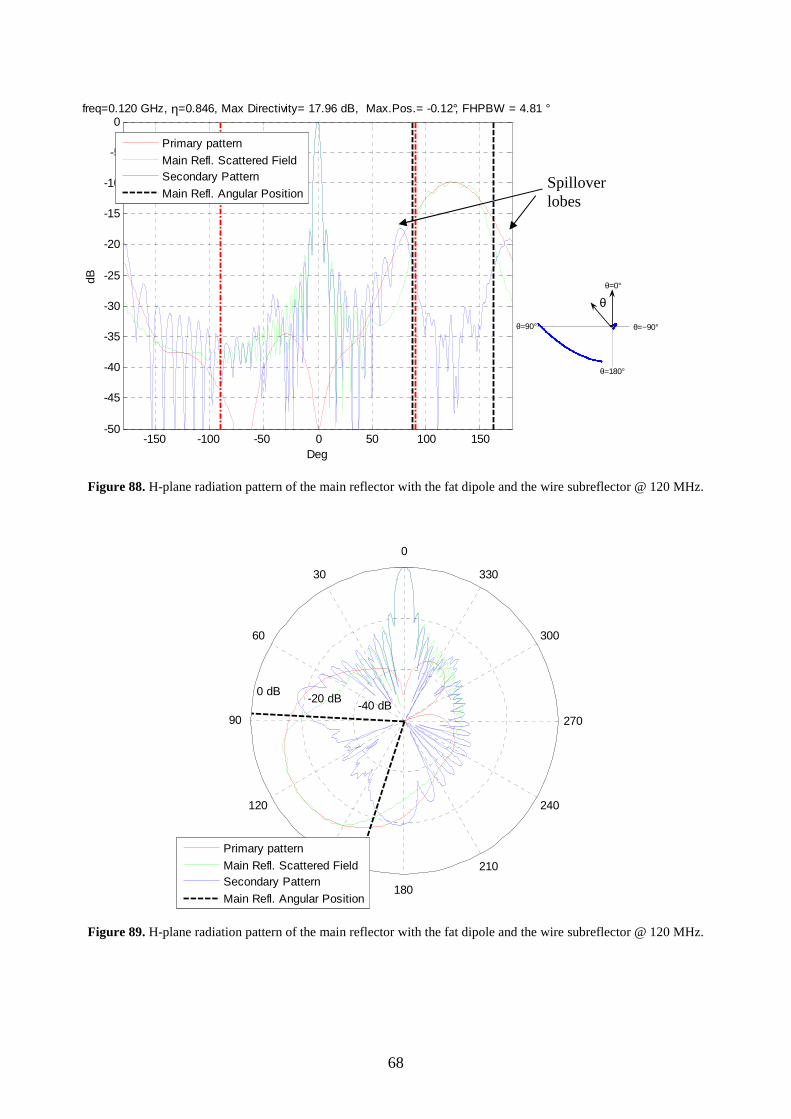
68

-150 -100 -50 0 50 100 150-50

-45

-40

-35

-30

-25

-20

-15

-10

-5

0

Deg

dB


Primary pattern



Figure 88. H-plane radiation pattern of the main reflector with the fat dipole and the wire subreflector @ 120 MHz.

-40 dB -20 dB

0 dB

30

210

60

240

90 270

120

300

150

330

180

0

Primary pattern




θθ=0°

θ=90°

θ=180°

θ=−90°

Spillover lobes

69

-150 -100 -50 0 50 100 150-50

-45

-40

-35

-30

-25

-20

-15

-10

-5

0

Deg

dB


Primary pattern




-40 dB -20 dB

0 dB

30

210

60

240

90 270

120

300

150

330

180

0

Primary pattern




θθ=0°

θ=90°

θ=180°

θ=−90°

Spillover lobes

70

Freq. MHz Width η (%)

HPBW (Deg)

Secondary Lobes (dB)

Spillover Lobes (dB)

120 18 4.4 -6 -10 Line source (no subref) 240 26 1.8 -11 -14

120 59 4.0 -14.7 -12 Commercial LPA 240 57 2.1 -15 -15

120 75 4.5 -13.5 -14 Custom LPA 240 65 2.2 -13.5 -15.5

120 85 4.8 -17.5 -17.5 Fat dipole + subreflector 240 84 2.7 -22 -26.5

Table 1. Comparison table between the different feed systems.

Conclusions

A low-cost feed system solution based on the LPA has been investigated. A commercial antenna was considered first. A width efficiency of approximately 60% and spillover lobes lower that -12 dB were found. On this basis, a custom LPA has been designed. It provides efficiency levels of 75% and 65% at the lower and upper ends of the 120-240 MHz bandwidth, respectively. The spillover lobes are below -14 dB. The comparison between these solutions and the ones that make use of a subreflector ([2] and [3]) highlights that the low-cost LPA feed system is feasible. However, it will not exploit the maximum capabilities of the Northern Cross E/W arm.

Since the spacing between the custom LPAs is 1.25 m, 18 antennas can be arranged in an array configuration which is approximately 22.5-m long. The outermost elements can be used as dummy elements providing a better similarity of the remaining 16 channels. It has to be remembered that the present wire subreflector working @ 408 MHz has to be removed in order to install the LPAs. Otherwise, a great distortion of the LPA radiation patterns would occur, reducing the overall efficiency and increasing the spillover lobes.

References

[6] G. Virone, R. Tascone, O. A. Peverini, G. Addamo, A. Olivieri, “EM Analysis of the

Northern Cross E/W Arm @ 408 MHz” IEIIT Technical Report EA061103 [7] G. Virone, R. Tascone, O. A. Peverini, G. Addamo, A. Olivieri, “Upgrade of the Northern

Cross E/W Arm for the 120÷240 MHz frequency band: general investigation and fat dipole solution” IEIIT Technical Report EA070410

[8] G. Virone, R. Tascone, O. A. Peverini, G. Addamo, A. Olivieri, “Upgrade of the Northern Cross E/W Arm for the 120÷240 MHz frequency band: dense array solution” IEIIT Technical Report EA070426

71

Technical Report

Measurements on the custom log periodic antenna

for the 120÷240 MHz upgrade of the Northern Cross E/W Arm

(Draft 1-EA/071220)

Giuseppe Virone, Giuseppe Addamo, Riccardo Tascone, Augusto Olivieri, Oscar Antonio Peverini

IEIIT-CNR




Torino 20th December 2007

72

This document reports the measurements carried out on two prototypes of the custom log periodic antenna described in the previous EA070719.

One of the prototypes is shown in Fig. 1 along with one of the designers in order to let the reader directly quantify the antenna dimensions.

Figure 92. Custom Log periodic antenna (without flange)

The designed antenna will be mounted on the E/W arm feed supporting structure by means of the metallic flange reported in Fig. 2.

Figure 93. Metallic flange to connect the antenna to the E/W arm supporting structure.

73

The reflection coefficient of both prototypes was measured with a vector network analyzer. The corresponding results are reported in Figs. 3 and 4, respectively. Both measurements are in good agreement with the simulated results confirming the reliability of the manufacturing procedure. The Aircell 5 coaxial cable which carries the signal from the tip of the antenna to the back is about 3.2 m long. Its measured transmission coefficient, which is reported in Fig. 5, can be used to compute the antenna losses.

0.1 0.12 0.14 0.16 0.18 0.2 0.22 0.24 0.26 0.28-30

-25

-20

-15

-10

-5

0

GHz

dB

Simulation

Measurement on prot. 1

Figure 94. Reflection coefficient (50 Ω) for prototype 1.

0.1 0.12 0.14 0.16 0.18 0.2 0.22 0.24 0.26 0.28-30

-25

-20

-15

-10

-5

0

GHz

dB

Simulation

Measurement on prot. 2

Figure 95. Reflection coefficient (50 Ω) for prototype 2.

74

0.1 0.12 0.14 0.16 0.18 0.2 0.22 0.24 0.26 0.28

-0.55

-0.5

-0.45

-0.4

-0.35

-0.3

GHz

dB

S21 cable

Figure 96. Transmission coefficient of a 3.2 m-long Aircell 5 coaxial cable.

The radiation pattern of one of the two prototypes has been characterized by means of an outdoor antenna test range. The prototype mounted on the fiberglass rotating pole is shown in Fig. 6.

Figure 97. Custom Log-periodic antenna mounted on the measurement fiberglass rotating pole.

75

The computed and measured H-plane radiation patterns are reported in Figs. 7-9. Since these patterns are in agreement with respect to the simulated data (also reported in EA070719), these antennas are suitable for the illumination of the E/W arm in the 120÷240 MHz frequency band. The E-plane radiation patters are instead reported in Figs. 10-12. In this case, the good agreement between simulations and measurements confirms the possibility of scanning the beam in the E-plane when these antennas are mounted in a linear array configuration, with or without the E/W main reflector. The discrepancies between simulations and measurements are due to the residual errors of the outdoor antenna test range.

-150 -100 -50 0 50 100 150-40

-35

-30

-25

-20

-15

-10

-5

0

Deg

dB

H-plane @ 120 MHz

Simulation

Measurement

Figure 98. H-plane radiation pattern @ 120 MHz.

76

-150 -100 -50 0 50 100 150-40

-35

-30

-25

-20

-15

-10

-5

0

Deg

dB

H-plane @ 180 MHz

Simulation

Measurement


-150 -100 -50 0 50 100 150-40

-35

-30

-25

-20

-15

-10

-5

0

Deg

dB

H-plane @ 240 MHz

Simulation

Measurement


77

-150 -100 -50 0 50 100 150-40

-35

-30

-25

-20

-15

-10

-5

0

Deg

dB

E-plane @ 120 MHz

Simulation

Measurement

Figure 101. E-plane radiation pattern @ 120 MHz.

-150 -100 -50 0 50 100 150-40

-35

-30

-25

-20

-15

-10

-5

0

Deg

dB

E-plane @ 180 MHz

Simulation

Measurement


78

-150 -100 -50 0 50 100 150-40

-35

-30

-25

-20

-15

-10

-5

0

Deg

dB

E-plane @ 240 MHz

Simulation

Measurement


Conclusion The measurements on the custom log periodic antenna prototypes confirmed the validity of both the design and the manufacturing technique. Therefore, the log periodic feeding array for the E/W arm of the Northern Cross in the 120÷240 MHz frequency band can be built using the developed antennas.

79

Technical Report


for the 120÷240 MHz and the 370÷430 MHz frequency bands:

multi-feed solution

(Draft 1-EA/080201)


IEIIT-CNR




Torino 1st February 2008

80

This document is an extension to the previous EA/070410 report entitled “Upgrade of the Northern Cross E/W Arm for the 120÷240 MHz frequency band: general investigation and fat dipole solution”. The main improvements with respect to the previous fat dipole solution consist of a smaller back side of the subreflector and a further dipole array working in the 370÷430 MHz frequency band. The former modification has been done in order to simplify the subreflector mounting on the existing feed supporting structure of the E/W arm of the Northern Cross, according to the meeting in Medicina on the 10th of May 2007. The second dipole array which is smaller and closer spaced than the fat dipole one is mounted as in Fig. 1 between the previous array and the back side of the subreflector. It has to be noted that the smaller array could be built using the dipoles of the present 408 MHz feed system. The present solution has been investigated in order to provide a low-cost upgrade of the Northern-Cross E/W arm with both the 120÷240 MHz and 370÷430 MHz frequency bands with a large -30°÷30° field of view. The back side reduction and the presence of the smaller array required a new design of the overall system. The main geometrical data are reported in Fig. 2. The subreflector aperture size w and length b are the same as in the original design. The larger and smaller arrays are arranged and labeled as in Fig. 3. The spacing of the larger array is the same as in the original design (1.25 m). The spacing of the smaller array is instead 0.368 m i.e. half wavelength @ 408 MHz.

Figure 104. Geometry of the subreflector with two dipole arrays. The larger ones work in the 120÷240 MHz frequency

band. The smaller dipoles work in the 370÷430 MHz frequency band.

81

Figure 105. Side view of the multi-feed structure. The aperture size w is 3 m, the total length b is 2.25 m, the size of the back side of the reflector a is 0.44 m, the distance dl of the larger dipole array from the back of the subreflector is 0.625

m and ds is 0.184 m.

Figure 106. Top view of the two dipole arrays. The spacing of the larger dipoles, labeled with L0, L+1, L-1, is 1.25 m.

The spacing of the smaller dipoles, labeled with S0, S+1, S+2, S-1, S-2, is 0.368 m.

Smaller Dipoles

Larger Dipoles

w a

b

dl

ds

L0 L+1 L-1

S0 S+1 S+2 S-1 S-2

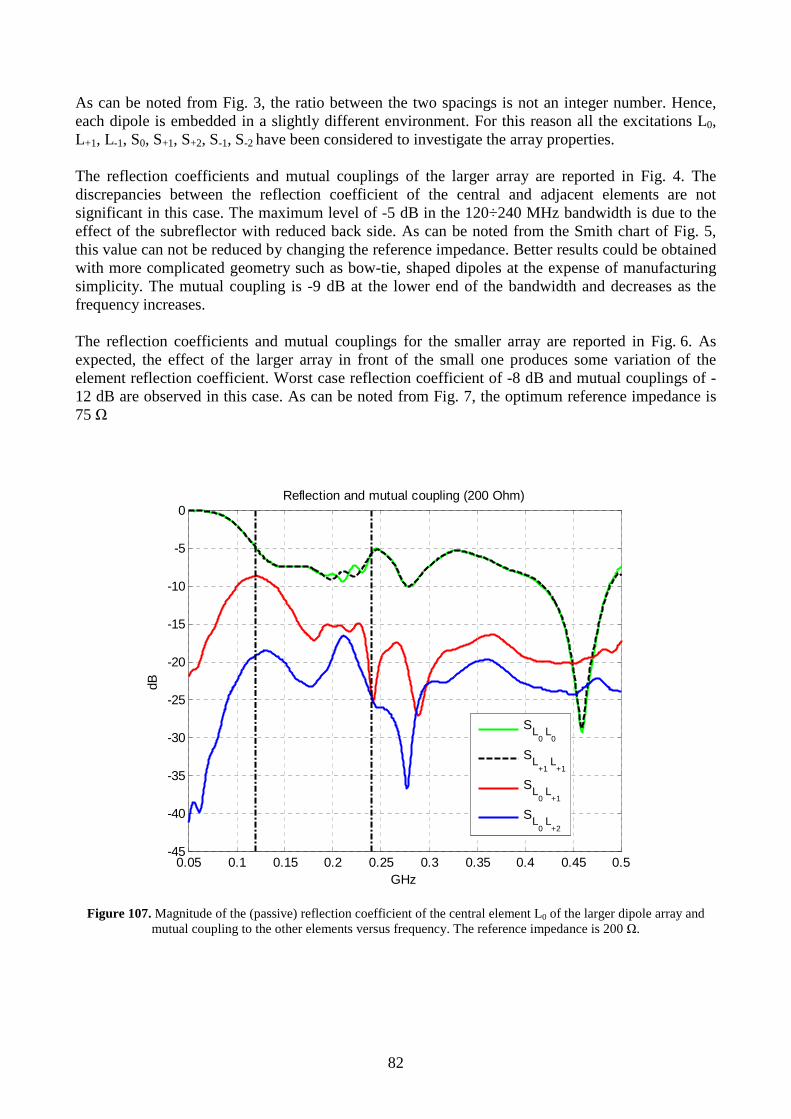
82

As can be noted from Fig. 3, the ratio between the two spacings is not an integer number. Hence, each dipole is embedded in a slightly different environment. For this reason all the excitations L0, L+1, L-1, S0, S+1, S+2, S-1, S-2 have been considered to investigate the array properties. The reflection coefficients and mutual couplings of the larger array are reported in Fig. 4. The discrepancies between the reflection coefficient of the central and adjacent elements are not significant in this case. The maximum level of -5 dB in the 120÷240 MHz bandwidth is due to the effect of the subreflector with reduced back side. As can be noted from the Smith chart of Fig. 5, this value can not be reduced by changing the reference impedance. Better results could be obtained with more complicated geometry such as bow-tie, shaped dipoles at the expense of manufacturing simplicity. The mutual coupling is -9 dB at the lower end of the bandwidth and decreases as the frequency increases. The reflection coefficients and mutual couplings for the smaller array are reported in Fig. 6. As expected, the effect of the larger array in front of the small one produces some variation of the element reflection coefficient. Worst case reflection coefficient of -8 dB and mutual couplings of -12 dB are observed in this case. As can be noted from Fig. 7, the optimum reference impedance is 75 Ω

0.05 0.1 0.15 0.2 0.25 0.3 0.35 0.4 0.45 0.5-45

-40

-35

-30

-25

-20

-15

-10

-5

0

GHz

dB

Reflection and mutual coupling (200 Ohm)

SL0 L

0

SL+1

L+1

SL0 L

+1

SL0 L

+2

Figure 107. Magnitude of the (passive) reflection coefficient of the central element L0 of the larger dipole array and

mutual coupling to the other elements versus frequency. The reference impedance is 200 Ω.

83

Figure 108. Smith chart plot of the (passive) reflection coefficient of the central element L0 of the larger dipole array.

The reference impedance is 200 Ω.

0.25 0.3 0.35 0.4 0.45 0.5-20

-18

-16

-14

-12

-10

-8

-6

-4

-2

0

GHz

dB

Reflection and mutual coupling (75 Ohm)

SS0 S

0

SS+1

S+1

SS+2

S+2

SS0 S

+1

SS0 S

+2

Figure 109. Magnitude of the (passive) reflection coefficient of the central element S0 of the smaller dipole array and

mutual coupling to the other elements versus frequency. The reference impedance is 75 Ω.

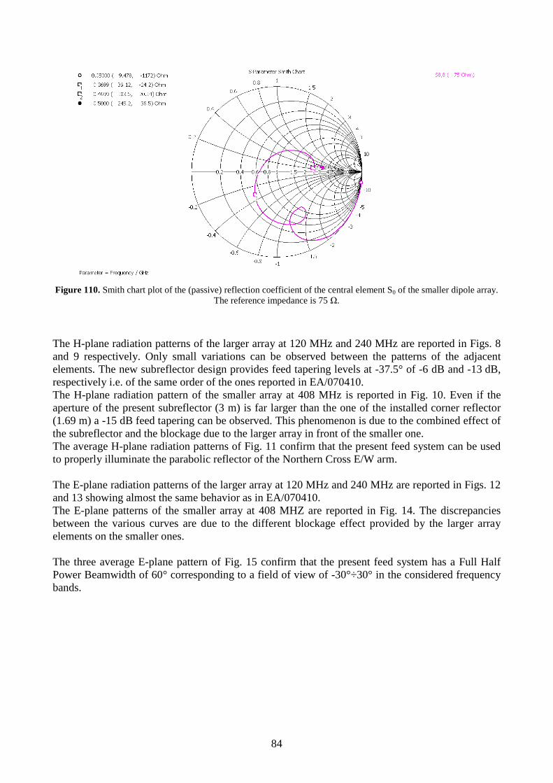
84

Figure 110. Smith chart plot of the (passive) reflection coefficient of the central element S0 of the smaller dipole array.

The reference impedance is 75 Ω.

The H-plane radiation patterns of the larger array at 120 MHz and 240 MHz are reported in Figs. 8 and 9 respectively. Only small variations can be observed between the patterns of the adjacent elements. The new subreflector design provides feed tapering levels at -37.5° of -6 dB and -13 dB, respectively i.e. of the same order of the ones reported in EA/070410. The H-plane radiation pattern of the smaller array at 408 MHz is reported in Fig. 10. Even if the aperture of the present subreflector (3 m) is far larger than the one of the installed corner reflector (1.69 m) a -15 dB feed tapering can be observed. This phenomenon is due to the combined effect of the subreflector and the blockage due to the larger array in front of the smaller one. The average H-plane radiation patterns of Fig. 11 confirm that the present feed system can be used to properly illuminate the parabolic reflector of the Northern Cross E/W arm. The E-plane radiation patterns of the larger array at 120 MHz and 240 MHz are reported in Figs. 12 and 13 showing almost the same behavior as in EA/070410. The E-plane patterns of the smaller array at 408 MHZ are reported in Fig. 14. The discrepancies between the various curves are due to the different blockage effect provided by the larger array elements on the smaller ones. The three average E-plane pattern of Fig. 15 confirm that the present feed system has a Full Half Power Beamwidth of 60° corresponding to a field of view of -30°÷30° in the considered frequency bands.

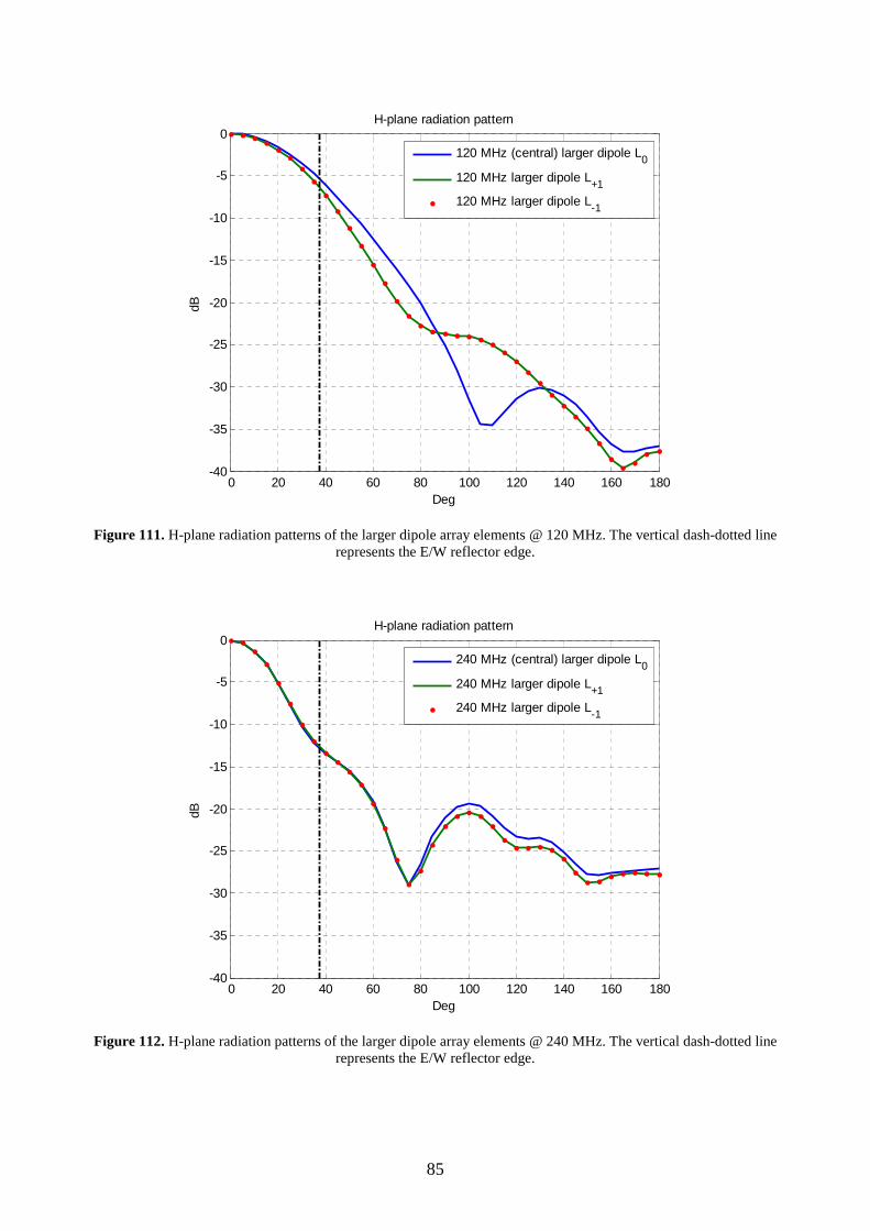
85

0 20 40 60 80 100 120 140 160 180-40

-35

-30

-25

-20

-15

-10

-5

0

dB

Deg

H-plane radiation pattern

120 MHz (central) larger dipole L0

120 MHz larger dipole L+1

120 MHz larger dipole L-1

Figure 111. H-plane radiation patterns of the larger dipole array elements @ 120 MHz. The vertical dash-dotted line

represents the E/W reflector edge.

0 20 40 60 80 100 120 140 160 180-40

-35

-30

-25

-20

-15

-10

-5

0

dB

Deg





Figure 112. H-plane radiation patterns of the larger dipole array elements @ 240 MHz. The vertical dash-dotted line


86

0 20 40 60 80 100 120 140 160 180-40

-35

-30

-25

-20

-15

-10

-5

0

dB

Deg


408 MHz (central) smaller dipole S0

408 MHz smaller dipole S+1


408 MHz smaller dipole S-1


Figure 113. H-plane radiation patterns of the smaller dipole array elements @ 408 MHz. The vertical dash-dotted line


0 20 40 60 80 100 120 140 160 180-40

-35

-30

-25

-20

-15

-10

-5

0

Deg

dB

H-plane average radiation pattern

larger dipoles 120 MHz

large dipoles 240 MHzsmaller dipoles 408 MHz

Figure 114. Average H-plane radiation patterns for the larger and smaller dipole arrays. The vertical dash-dotted line


87

-150 -100 -50 0 50 100 150-40

-35

-30

-25

-20

-15

-10

-5

0

dB

Deg

E-plane radiation pattern




Figure 115. E-plane radiation patterns of the larger dipole array elements @ 120 MHz. The vertical dash-dotted line

represents the required -30°÷+30° field of view.

-150 -100 -50 0 50 100 150-40

-35

-30

-25

-20

-15

-10

-5

0

dB

Deg







88

-150 -100 -50 0 50 100 150-40

-35

-30

-25

-20

-15

-10

-5

0

dB

Deg


408 MHz (central) smaller dipole S0







-150 -100 -50 0 50 100 150-40

-35

-30

-25

-20

-15

-10

-5

0

Deg

dB

E-plane average radiation pattern

larger dipoles 120 MHz

large dipoles 240 MHzsmaller dipoles 408 MHz

Figure 118. Average E-plane radiation patterns for the larger and smaller dipole arrays. The vertical dash-dotted line


collection of technical reports on the electromagnetic ... ieiit.pdf · dell’informatizione e...

Documents