coherence in classical electromagnetism and quantum optics
TRANSCRIPT

Coherencein
Classical Electromagnetism
andQuantum Optics
Hanne-Torill Mevik
Thesis submitted for the degree ofMaster in Physics
(Master of Science)
Department of PhysicsUniversity of Oslo
June 2009


Acknowledgements
It sure hasn’t been easy to explain to friends, family or even fellow students whatmy thesis is about. To be honest, most of the time I myself had no clue. Although, Iguess there is nothing unique about neither me nor this thesis in that regard. But nowthe day finally has arrived. The day when the final Ctrl-z’s and Ctrl-s’s has been typedand it’s time for Ctrl-p. This is also the last day that I can rightly call myself a student,at least as far as Lånekassen is concerned. Four years, 10 months and a few days laterafter first setting foot on Blindern Campus, with the contours of my posterior firmlyimprinted on the seat of my chair, the credit is not mine alone. My heartfelt thanks goesto...
... My mother whom I owe everything. Thank you for always being proud of meeven though I didn’t become a lawyer or a surgeon. Her unwavering faith in me madesure I never for one second hesitated in enrolling at the Physics Department, where Iwas greeted by...
... The 4 o’clock Dinner Gang (you know who you are!). An infinite well of braindead topics for discussion over any type of beverages and/or edibles. Without you Iwould never have met...
... Lars S. Løvlie, balm for my soul. His invaluable moral support and last minuteproof reading ensured that I could present this thesis in its never-to-be-edited-againform to...
... My supervisor, Jon Magne Leinaas. Infinite patience incarnate, thank you for theinteresting topic which has been thoroughly enjoyable to delve into and for the gentlenudges to put me back on track when I diverged. I frequently say that there is no fun ineasy achievements (a meagre comfort at most), and when the MDD1 set in...
... Joar Bølstad was there to listen to my whining over a steaming cup of Earl Grey.We made it to graduation day! :)
You all put the “fun” in “student loan”! (Hey, wait a minute...)
Blindern, Oslo .htm2nd of June 2009
1Master student’s Depression Disorder: a mental disorder characterized by an all-encompassing lowmood accompanied by low self-esteem, and loss of interest or pleasure in normally enjoyable activities.
iii

Abstract
This thesis is a study of coherence theory in light in classical electromagnetism andquantum optics. Specifically two quantities are studied: The degree of first-ordertemporal coherence, which quantifies the field-field coherence, and the degree ofsecond-order coherence, quantifying the intensity-intensity coherence. In the first partof the thesis these concepts are applied to classical electric fields; to both the idealplane wave and to chaotic light. We then study how they can be measured using twointerferometer technologies from optical astronomy, specifically with the Michelsonstellar interferometer and the intensity interferometer.
In the second part we define the quantum degrees of first- and second-order coher-ence. These are calculated for light in a quantum coherent state, in a Fock state and forlight in a mixed thermal state. The results for the coherent state and the thermal stateare found to be analogous to those obtained for the ideal plane wave and chaotic light,respectively, from the classical coherence theory seen in the first part.
We proceed to investigate the properties of the three-level laser with the aim ofshowing that far above threshold it develops similar photon statistics and values forthe degrees of first- and second-order coherence, to light in a coherent state. Themechanism of phase-drift in the laser is also looked into. Subsequently the Mølmer-model is discussed, where it is demonstrated that the coherent state is not a necessaryconstruct, but merely a convenient one, in describing phenomena in quantum optics.
v


Contents
Introduction 1
I Coherence in classical electromagnetism 3
1 Classical electromagnetism and coherence 5
1.1 Classical description of light . . . . . . . . . . . . . . . . . . . . . . 5
1.2 Coherence . . . . . . . . . . . . . . . . . . . . . . . . . . . . . . . . 10
1.3 The degree of first-order coherence . . . . . . . . . . . . . . . . . . . 14
1.4 The degree of second-order coherence . . . . . . . . . . . . . . . . . 20
1.5 Summary and discussion . . . . . . . . . . . . . . . . . . . . . . . . 25
2 Measuring coherence with interferometers 27
2.1 The apparent angular diameter of a binary star . . . . . . . . . . . . . 28
2.2 The Michelson stellar interferometer . . . . . . . . . . . . . . . . . . 32
2.3 The intensity interferometer . . . . . . . . . . . . . . . . . . . . . . 37
2.4 Comparison and discussion . . . . . . . . . . . . . . . . . . . . . . . 45
II Coherence in quantum optics 53
3 The quantised electric field and quantum coherence 55
3.1 Quantisation of the electromagnetic field . . . . . . . . . . . . . . . . 55
3.2 The quantum degrees of first- and second-order coherence . . . . . . 60
3.3 The Quantum Hanbury Brown-Twiss effect . . . . . . . . . . . . . . 62
3.4 Coherent states of the electric field . . . . . . . . . . . . . . . . . . . 65
3.5 Summary and discussion . . . . . . . . . . . . . . . . . . . . . . . . 70
vii

viii Contents
4 Calculations of the quantum degrees of coherence 73
4.1 Light in a coherent state . . . . . . . . . . . . . . . . . . . . . . . . . 73
4.2 Light in a Fock state . . . . . . . . . . . . . . . . . . . . . . . . . . 76
4.3 Light in a mixed thermal state . . . . . . . . . . . . . . . . . . . . . 78
4.4 Discussion . . . . . . . . . . . . . . . . . . . . . . . . . . . . . . . . 84
4.5 Photon states and their distinctive traits . . . . . . . . . . . . . . . . 85
5 Coherence in the laser 91
5.1 The equation of motion for the three-level model . . . . . . . . . . . 92
5.2 The diagonal elements and laser photon statistics . . . . . . . . . . . 98
5.3 The degrees of first- and second-order coherence . . . . . . . . . . . 103
5.4 Phase drift . . . . . . . . . . . . . . . . . . . . . . . . . . . . . . . . 104
5.5 Summary and discussion . . . . . . . . . . . . . . . . . . . . . . . . 111
6 Unexpected coherence 113
6.1 The Mølmer-model . . . . . . . . . . . . . . . . . . . . . . . . . . . 113
6.2 The numerical recipe . . . . . . . . . . . . . . . . . . . . . . . . . . 118
6.3 The results of the simulation . . . . . . . . . . . . . . . . . . . . . . 118
6.4 Summary and discussion . . . . . . . . . . . . . . . . . . . . . . . . 123
7 Concluding remarks 125
A Determining the statistical properties of chaotic light 129
A.1 Collision (pressure) broadening . . . . . . . . . . . . . . . . . . . . . 129
A.2 Doppler broadening . . . . . . . . . . . . . . . . . . . . . . . . . . . 131
B Selected tedious calculations 134
B.1 The energy of the classic radiation field . . . . . . . . . . . . . . . . 134
B.2 The Lie formula . . . . . . . . . . . . . . . . . . . . . . . . . . . . . 135
B.3 Solving the eigenvalue problem . . . . . . . . . . . . . . . . . . . . . 136
C Source code listings 138
C.1 Script for calculating coherences . . . . . . . . . . . . . . . . . . . . 138
C.2 Script for calculating Monte Carlo quantum jumps . . . . . . . . . . 141
References 145

Introduction
Optics may very well be the oldest field in physics, with evidence of systematic (ifnot scientific by modern standards) writings dating back to antiquity and the Greekphilosophers and mathematicians. Two millennia later the field is still in full vigour,especially these last six decades, where new discoveries keep pushing the frontiers. In1704 Sir Isaac Newton gave out Opticks, which is considered one of the greatest worksin the history of science. The geometrical optics of this time treated the light as raystravelling in straight lines until bending through refraction, and white light rays couldbe split into colours by a prism. James Clerk Maxwell (1873) succeeded in combiningthe then separate theories of electricity and magnetism, which by conjecture led to lightwaves being electromagnetic waves. Since then and up until today the very successfullanguage of optics has been the theory of electromagnetism, or the more contemporary,semi-classical theory in which the fields are treated as electromagnetic waves and matteris treated with quantum mechanics.
However, the validity of the electromagnetic theory of light is limited. While it iscapable of explaining the phenomena dealing with propagation of light, it fails whenit comes to the finer features of the interaction between light and matter, such as theprocesses of emission and absorption. Here the theory must be replaced by quantummechanics. The advent of quantum mechanics also brought with it the view that lightis quantised as photons. Experiment after experiment confirmed both the particle andthe wave description of light, leading to the “middle-ground” concept of the wave-particle-duality. The wave-particle duality says that all matter and energy exhibits bothwave-like and particle-like properties and it has since it was first uttered been imprintedin the minds of (at least three) generations of physicists. Apparently the particle aspectof light, the photon view, became so deeply entrenched that it excluded the wave aspectalmost entirely, at least for the visible part of the electromagnetic spectrum. Theseinflexible mindsets only grudgingly bent to include the wave view when the intensityinterferometer for optical wavelengths was invented by R. Hanbury Brown and R. Twissin 1956.
The problem was that the intensity interferometer was designed to measure coher-ence, but coherence was thought to be a property related to the classical electromagneticwave, leading to interference. And this was accepted for radio waves, but not for theoptical wavelengths as the light was believed to be so energetic as to be quantised in arelative small number of photons. Even so, Hanbury Brown and Twiss made successfulmeasurements; Evidently a better understanding of the coherence properties of light
1

2 Contents
and their effect on the interaction between light and matter was required. The classicalcoherence theory has been around since classical electromagnetism was formulated,and it accounts well for phenomena like interference. But the quantum coherence theorywas not fully formulated until Roy J. Glauber in 1963 presented the “coherent state” asparticularly appropriate for the quantum treatment of optical coherence. Incidentally,the intensity interferometer could now be fully described by both the classical and thequantum theory. But it was mainly the development of the laser in the 1960s that ledto the emergence of quantum optics as a new discipline. The laser was a completelynew type of light source that provided very intense, coherent and highly directionalbeams which very closely resembled ideal plane waves. Recent “quantum leaps” inexperimental techniques the last half of the 21st century has enabled measurements ofsingle photons, and while the semi-classical theory of light is in good agreement withexperiments on high frequency light, it yields incorrect results for experiments relyingon photon statistics.
The central theme to this work is coherence in light. What is coherence and howis it quantified, calculated, measured? What is the difference between coherent lightand incoherent light? Can light be something in between? Can coherence be explainedby both classical electromagnetism and quantum mechanics? Are the explanationsequivalent? Does it matter which statistical properties the light has?
The attempt to answer these questions is divided into two parts; First we takeon coherence in classical terms where the mathematical description is developed inchapter 1, before applying the coherence theory to concrete cases. We have chosen twoexamples from optical astronomy for this purpose, where coherence is used to measurethe angular diameter of a binary star, namely the Michaelson stellar interferometer andthe intensity interferometer is explained in chapter 2. From the historical overview aboveit should be apparent why the intensity interferometer is interesting. The Michelsonstellar interferometer then serves as a good contrast as it employs the less “controversial”classical coherence-effect of electric field interference.
In the second part we tackle the coherence problem on the quantum side of theballpark. This requires the quantised electric field and the density operator, both ofwhich are derived in chapter 3, to subsequently be put to use in the quantum coherencetheory. In chapter 4 coherence is calculated for light in the coherent state, the Focknumber state and the mixed thermal state. Chapter 5 is devoted to the principles of thelaser. There we investigate its photon statistics and its coherence properties in orderto see why the laser under certain conditions is a good approximation to the classicalideal plane wave. Finally, in chapter 6 we look into the Mølmer-model to see whether itis really necessary to use the coherent state to explain the occurrence of coherence inlight.
For this work to be intelligible for students in their late bachelor’s or early mas-ter’s stage, some introductory material has been included in detail. For example, thederivation of the free classical electric field (which clarifies what is meant by a mode ofthe field) and the quantisation of the electric field (for the explicit relation between thecomplex classical field amplitude and the quantum harmonic oscillator operators).

Part I
Coherence in classicalelectromagnetism
3


Chapter 1
Classical electromagnetism andcoherence
First on the agenda is to recapitulate the basics of the electromagnetic theory thatpertains to the goal of this thesis: examining the concept of coherence in light, usingboth classical electric field theory and the quantum mechanical photon description. Inthe present chapter we will use Maxwell’s equations to derive a form of the electricfield which will be used in the discussion of coherence in section 1.2. It will also comein handy when we move on to the quantum theory in chapter 3 and need to work withthe quantised electric field.
The goal of section 1.2 is to develop an understanding of coherence and of the twocorrelation functions famously known as the degree of first-order temporal coherenceand the degree of second-order temporal coherence. The former tells us how the electricfield measured at two points in time is correlated, and the latter quantifies the correlationof the electric field intensity in a similar way. We will also look into how these twofunctions are related to each other, and how the Wiener-Khinchin theorem relates thedegree of first-order temporal coherence to the power spectrum of the radiation field.
This will all culminate in chapter 2 with the application of the degree of first-and second-order temporal coherence on two seemingly similar, but as we will see,fundamentally different, stellar interferometers.
1.1 Classical description of light
In this part we will take the semi-classical approach, in the sense that particles aredescribed by quantum mechanical wave functions while the electromagnetic field istreated as classical waves. To find the required expressions for the electromagnetic fieldwe start with Maxwell’s equations.
5

6 Classical electromagnetism and coherence
1.1.1 Maxwell’s equations
In the presence of a charge density ρ(r, t) and a current density j(r, t), the electric andmagnetic vector fields E and B satisfy Maxwell’s equations 1
∇ ·E = ρ/ε0 (1.1a)
∇ ·B = 0 (1.1b)
∇×E = −∂B∂t
(1.1c)
∇×B =1c2
∂E∂t
+ µ0J (1.1d)
where we have used SI units, and µ0 is the magnetic constant and ε0 the electricconstant such that µ0ε0 = c−2. As usual c denotes the speed of light in vacuum2.We will consider the case of the free field, i.e., in absence of charges and currents,equivalent to setting ρ = 0 and J = 0.
Gauss’ law Eq. (1.1a) describes how the electric field will behave in the vicinityof an electric charge: the field lines points towards a negative charge and away froma positive charge. Gauss’ law for magnetism Eq. (1.1b) tells us that unlike electricity,there is no “positive” or “negative” particles that can make the magnetic field tend topoint towards or away from them. Instead these particles must come in pairs of bothnegative and positive. Faraday’s law of induction Eq. (1.1c) says that a change in themagnetic field can induce an electric field, and Ampere’s law Eq. (1.1d) shows how achange in the electric field or an electric current can induce a magnetic field.
From Gauss’ law for magnetism and Faraday’s law of induction one can define thescalar and the vector potentials φ(r, t) and A(r, t) as follows
B = ∇×A, E = −∇φ− ∂A∂t
. (1.2)
This does not determine the potentials uniquely, however, since there are many differentchoices of φ and A that will yield the same E and B. To cope with the redundantdegrees of freedom in the field variables we can choose the typical gauge
∇ ·A = 0. (1.3)
This constraint on the vector potential is known as the Coulomb gauge and it has theadvantage that it decouples the equations for φ(r, t) and A(r, t). Eq. (1.3) is also calleda transverse gauge, since a vector field satisfying it is a transverse wave. If at point r inspace, at time t, the vector potential is
A(r, t) =∑k
Akei(k·r−ωkt)
1 In this work all vectors are in boldface. Also the del operator is
∇ ≡ exd
dx+ ey
d
dy+ ez
d
dz
where (ex, ey, ez) are unit vectors in the respective coordinate directions.2The speed of light in vacuum is c = 3.0 · 108 m/s.

1.1 – Classical description of light 7
where A0 is the field amplitude, k is the wave vector and ωk = |k|c is the angularfrequency, then
∇ ·A ∝∑k
k ·Ak = 0, (1.4)
which means that A is perpendicular to the direction of the propagation k of the wave.The electric and magnetic fields E and B can be expressed in terms of the transversefield A, and are therefore themselves transverse fields. A is often referred to as theradiation field and we will frequently use the term “radiation field”. However, as themajority of the calculations in this work involves the electric field, it is implied that weare interested in just the electric part of the radiation field. After all, even if technicallythe radiation field is composed of both an electric and a magnetic component, we canalways choose a reference frame where we only perceive the electric field.
1.1.2 The free classical electric field
At any given instant in time the electric field E must be specified at every point xin space. But this implies that the electric field has an infinite number of degrees offreedom. To work around this problem we consider the radiation to be confined in acubic cavity with sides of length L and periodic boundary conditions imposed at thewalls of the cavity. We can then represent the electric field as a Fourier series, with aninfinite, but countable, number of Fourier coefficients.
From Maxwell’s equations we can take the curl of Eq.(1.1c) and then use Eq.(1.1a)while inserting Eq.(1.1d). A key ingredient is the relation
∇× (∇×E) = ∇(∇ ·E)−∇2E.
The end result shows that E(r, t) satisfies the wave equation
∇2E− 1c2
∂2E∂t2
= 0. (1.5)
The electric vector field can be split up in a scalar and a vector part like
E =∑k
∑λ
εkλEkλ (1.6)
where Ekλ is the scalar electric field of mode k, the meaning of which will soon beapparent, and εkλ is the unit polarisation vector of mode k in direction λ. It is prettystraight forward to solve the partial differential equation, especially since the boundaryconditions on the cavity should be independent of time. One can then do a separationof the variables r and t, e.g.,
Ekλ(r, t) = Xkλ(r)akλ(t). (1.7)
which leads to two ordinary differential equations for each mode k
1Xkλ
∇2Xkλ =1
c2akλ
∂2akλ∂t2
= −|k|2. (1.8)
8 Classical electromagnetism and coherence
We can assume a running-wave solution, in which case the boundary conditions willgive
Xkλ(r) = εkλeik·r (1.9)
Then the scalar electric field can be written on the form
Ekλ(r, t) = akλ(t)eik·r + a∗kλ(t)e−ik·r. (1.10)
This form ensures that the electric field is real: E = E∗. The periodic boundaryconditions are ensured by
k = (kx, ky, kz) =2πL
(nx, ny, nz), nx, ny, nz = 0,±1,±2, . . . (1.11)∑k is understood to be the sum over the integers nx, ny, nz and the set of numbers
(nx, ny, nz) defines a mode of the electromagnetic field. So later when we talk aboutone mode of the electric field, we mean one of the possible solutions to the electric fieldwave equation.
With εkλ as the unit polarization vector we see from Eq. (1.1a) that the electric fieldis purely transverse since[
∇Ekλ(r, t)]· εkλ = 0 ⇒ k · εkλ = 0. (1.12)
This means that there are only two independent polarization directions of εk for each k.These two unit vectors are mutually perpendicular:
εkλ · εkλ′ = δλλ′ , λ, λ′ = 1, 2. (1.13)
The electric field is now essentially expanded as a Fourier series
E(r, t) =∑k
∑λ
(~ωk
2ε0L3
)1/2
εkλ
[akλ(t)eik·r + a∗kλ(t)e−ik·r
](1.14)
The factor (~ωk/2ε0L3)1/2 is a convenient choice3. The modal components of E mustsatisfy the wave equation Eq. (1.5), so we insert Eq. (1.14) into it with the result thateach mode k must fulfill(
∇2 − 1c2
∂2
∂t2
)(~ωk
2ε0L3
)1/2
εkλakλ(t)eik·r = 0 (1.15)
giving
∂2
∂t2akλ(t) + ω2
kakλ(t) = 0. (1.16)
This is the equation for the harmonic oscillator for the normal mode k of the radiationfield. A convenient solution is
akλ(t) = akλe−iωkt, (1.17)
3The Planck constant is defined as h = 2π~ = 6.626 · 10−34 Js.

1.1 – Classical description of light 9
where ωk = c|k| and akλ is the initial amplitude at time t = 0. The electric field thenbecomes
E(r, t) =∑k
∑λ
(~ωk
2ε0L3
)1/2
εkλ
[akλe
i(k·r−ωkt) + a∗kλe−i(k·r−ωkt)
]. (1.18)
Now that we have an expression for the free electric field we can use Eq. (1.1c) tofind the magnetic field. The fairly straight forward calculation gives
B(r, t) =∑k
∑λ
(~ωk
2ε0L3
)1/2 k× εkλ
ωk
[akλe
i(k·r−ωkt)+a∗kλe−i(k·r−ωkt)
]. (1.19)
With the expressions for E and B in place, we have the solution for the transverseelectromagnetic waves in free space. The total energy of the radiation field in the cavitywith volume V = L3 is
HR =12ε0
∫V
(E2 + c2B2)dr. (1.20)
This calculation is carried out in Appendix B.1 and the resulting total radiative energyis
HR =∑k
∑λ
12
~ωk(akλa∗kλ + a∗kλakλ) =∑k
∑λ
~ωkakλa∗kλ (1.21)
i.e., a sum of the time-independent contributions from field amplitudes of the individualmodes k. The field amplitudes akλ and a∗kλ are classical coefficients which commute,so the two terms can be added to form one single term. This form for the radiativeenergy suggests an analogy between the mode amplitudes akλ, a∗kλ and an ensembleof the individual one-dimensional harmonic oscillators. From chapter 3 and on, weneed the quantised radiation field, which will be found by replacing the classicalharmonic oscillator with the corresponding quantum mechanical harmonic oscillator,and converting the classical field variables into field operators. Eq. (1.21) will showthe conversion from the classical electric amplitudes to the quantum mechanical modeoperators.
1.1.3 The Poynting vector
The electric field comes in many shapes and forms depending on what will be mostsuitable for the pending calculation. In the above we have found a form of the electricfield which will be very convenient when we later move on to the quantum part ofquantum optics, but in the immediate future we do not need such a complicated form ofthe field and we can stick to just the positive frequency part
E(r, t) =∑k
∑λ
(~ωk2L3
)1/2
εkλakλei(k·r−ωkt) (1.22)

10 Classical electromagnetism and coherence
This is justified by the fact that E(r, t) is real and that the negative frequency part doesnot contain any new information that is not already provided by the positive frequencypart since they are the complex conjugated of each other. While we know that theelectric field is real; our eyes detect it, the nerve endings in our skin prickles fromthe intensity of it; it is a matter of mathematical convenience to do calculations with acomplex electric wave function. However, when we in the end need the real field, it isonly a question of adding the negative frequency part back into Eq. (1.22).
The intensity of the complex electromagnetic field is given by the Poynting vector
S =12ε0c
2(E×B). (1.23)
From Eqs. (1.14) and (1.19) we have for a selected mode
Bk =kkc×Ek (1.24)
giving
Sk =12εc2Ek ×
(kkc×Ek
)=
12ε0c
[kk
(Ek ·Ek)−Ek
(kk·Ek
)]=
12ε0c|Ek|2
kk, (1.25)
where the rightmost term on the second line is zero due to Eq. (1.12).
It is impractical, or even impossible, to resolve the oscillations in the electric fieldin Eq. (1.22) that occur at the frequency ωk. According to [1], a good experimentalresolving time is of the order of 10−9 s, which is far too long to detect oscillations atvisible frequencies (e.g. ωk ∼ 1015Hz). It is therefore more meaningful to instead useI(t) in the calculations. The overbar denotes the cycle-averaged intensity, which meansthat the theoretical expression for the intensity has been averaged over one period ofthe wave,
I(t) = |S| = 1T
∫T
12ε0c|E(r, t)|2dt =
12ε0c|E(r, t)|2. (1.26)
1.2 Coherence
This section is devoted to explaining what coherence is and what it means for light tobe coherent. This will pave the way for chapter 2 where we will investigate how onecan utilise the coherence of light to determine the diameter of a binary star with stellarinterferometers.
Interferometers have their name from the effect they exploit to study the propertiesof light, namely interference. As we are taught early on in undergrad-hood, interferencecreates a new wave pattern when two or more waves are superposed on each other.

1.2 – Coherence 11
The interference effect is due to the relative difference in the phases of the superposedwaves. Depending of the relative phase, two waves will either interfere constructively(difference of 2mπ, m is an integer) or destructively (difference of 2(m+ 1)π). If thewaves have the same frequency with a constant relative phase difference, they are saidto be coherent.
The classical description of the electric part of an ideal plane light wave is
E(r, t) = E0ei(k·r−ωt). (1.27)
From now on for the rest of this work, we for simplicity assume that the field is linearlypolarized in one direction and is thus scalar. The ideal plane wave is perfectly coherent,which means that if we know the amplitude and phase at one time, we can deduce if forall times. To create interference we could for instance split the ideal wave in two, andlet each part follow two different paths until they are brought back together again. Ifthe paths have different lengths, the path difference ∆d = cτ (where τ can be calledthe time delay) will introduce a relative phase difference of ∆φ = ωτ between the twofields when they are superposed. Changes in the path difference, i.e., in τ , will revealitself in transitions between constructive and destructive interference.
In practice, however, a single free atom does not at all radiate ideal monochromaticlight, but rather the generalised field
E(r, t) = |E(r, t)|eiφ(r,t). (1.28)
where φ(r, t) contains some range of angular frequencies ∆ω. So if the relative phaseof the superposed fields is not constant overall, but only approximately constant withina time interval τc, the fields are partially coherent. The frequency spread in the sourceleads to the possibility that intensity maxima for one frequency coincides with theminima of another. In effect this washes out the interference pattern and imposespractical limits on the maximum time delay τ that will give an observable interferencepattern. So in a sense coherence is a measure of the frequency stability of the light,and it is quantified by the coherence time τc. From this we obtain the coherence lengthdc = cτc. If we know the phase of the wave at some position z at time t, then we willknow the phase at the same position at t+ τ with high certainty if τ τc, or with verylow certainty if τ τc.
To quantify coherence we can calculate the correlation. We will focus on two typesof correlations of the electric field, the first of which is the first-order correlation of onefield at two points in space that are separated by a distance d = cτ . The equivalentwould be one field at the same point in space, measured at two times t and t + τ . Inboth cases τ can be seen as a delay in the measurements. Secondly we will look at thesecond-order correlation of the field intensity at two points in space, also separated byd = cτ . Much of this chapter follows the discussion in [1].
It should be pointed out that there are in general two types of coherence: temporaland spatial coherence. We have made a choice to focus on temporal coherence; it is inprinciple simpler and more intuitive than spatial coherence and the examples we willlook at in chapter 2 will work just fine without the added complications.

12 Classical electromagnetism and coherence
(a)
(b) (c)
Figure 1.1: Visualisation of different types of coherent light. (a) Light with both infinitecoherence length lc and infinite coherence area Ac. (b) Spatially coherent lightwith infinite coherence area Ac, but only partially temporal coherence as seenfrom the finite coherence length lc. (c) Partially spatial and temporal coherentlight, with finite coherence length and area.
Nevertheless, a few words are well spent on explaining what is meant by temporaland spatial coherence. The ideal wave case has an infinite temporal coherence lengthlc and an infinite spatial coherence area Ac, as can be seen in Fig. 1.1(a). Temporalcoherence is a measure of how well correlated the phases of a light wave are at differentpoints along the direction of propagation. In that sense one could call this a longitudinalcoherence. Sampling the field at time t, how well could you then predict the amplitudeand phase a time τ later? This prediction would be pretty accurate as long as τ iswithin the coherence time τc of the light, which is infinite for the ideal wave. The moretemporally coherent the light is, the more monochromatic it is.
Spatial coherence is in contrast a measure of how well correlated the phases areat different points normal to the direction of propagation. In that respect one couldcall it transverse coherence. The more spatially coherent the light is, the more uniform

1.2 – Coherence 13
the wave front is. A perfect point source would be perfectly spatially coherent, but inpractice of course, a real source must have a finite physical size and as such spatialcoherence should only be neglected in gedankenversuche and master’s theses.
The coherence areaAc is defined as the length of the coherent wave front multipliedwith the wavelengths where the profile of the field is unchanged. In order to observeinterference when the light passes through two slits, the coherence area Ac must belarge enough that the wave front is more or less constant, otherwise the interferencepattern is washed out. Light can be temporally and/or spatially coherent; The one doesnot preclude nor imply the other. Examples can be seen in Fig. 1.1(b), where light isspatially coherent, but have only partial temporal coherence, while in Fig. 1.1(c) thelight have partial spatial and temporal coherence4.
1.2.1 Different types of light
In this work we will deal with mainly two types of light sources: Those that emitcoherent light and those that emit chaotic light. The laser5 is thought to be a coherentlight source in that it emits (mostly) monochromatic light with a constant relative phase.To really understand the laser we need to use quantum theory. This is postponed untilchapter 5 in the second part, dedicated to the laser and its intriguing properties.
Chaotic sources, like for example the filament lamp or the sun, are so-called thermalsources where the radiation is the result of high temperature. They consist of a verylarge number of atoms which radiates almost independently of each other, leadingto the term chaotic. The frequency and phase of the emitted light is determined bythe unstable energy levels of the atoms, the statistical spread in atomic velocities andrandom collisions between atoms. Thus the statistical properties of chaotic light areprofoundly different from that of coherent light.
We adopt the common convention that chaotic light is ergodic. If a random processis ergodic, any average calculated along a sample function (i.e., a time average ofthe electric field emitted by a single atom) must equal the same average calculatedacross the ensemble (i.e., a simultaneous ensemble average over the ν equivalent atoms).A less restrictive demand is that the statistics governing chaotic light is wide-sensestationary, meaning that the following two conditions are met
1. E[u(t)] is independent of t.
2. E[u(t1)u(t2)] is independent of τ = t2 − t1.
where E[] denotes the expectation value of the random process6 u(t) [2]. So by wide-sense stationary it is meant that the random fluctuations in the light are governed byinfluences that does not change with time.
4Please allow for artistic interpretation!5Light Amplification by Stimulated Emission of Radiation.6The definition of a random process is to assign the real valued function u(A; t), at independent
variable t, to an event A. In our case u(t) would be the real electric field produced by a source emission attime t.

14 Classical electromagnetism and coherence
1.3 The degree of first-order coherence
The degree of first-order temporal coherence of light is useful for quantifying thecoherence of either two electric fields simultaneously at two points in space, or of onefield at one point in space at two different times. It is defined as
g(1)(τ) =〈E∗(t)E(t+ τ)〉〈E∗(t)E(t)〉 (1.29)
which is a normalised version of the first-order correlation function for the electric fieldsampled at times t and t+ τ
〈E∗(t)E(t+ τ)〉 =1T
∫ t+T/2
t−T/2E∗(t′)E(t′ + τ)dt′. (1.30)
The angle brackets denotes time averaging. If the light has wide-sense stationarystatistics the correlation only depends on the time delay τ between the two field values.In that case Eq. (1.30) is independent of the starting time t, at least in so far that theinterval T is much longer than the characteristic time scale of the fluctuations. Thecharacteristic time is also called the coherence time, denoted by τc.
From
〈E∗(t)E(t− τ)〉 = 〈E∗(t)E(t+ τ)〉∗ = 〈E(t)E∗(t+ τ)〉
it follows that
g(1)(−τ) = g(1)(τ)∗. (1.31)
By the definition in Eq. (1.29) it is obvious that for τ = 0
g(1)(0) = 1, (1.32)
which means that at zero delay time τ , the light is first-order coherent and for delaytimes τ τc it will remain approximately coherent.
For chaotic light (of any kind) the field correlations vanish for delay times muchlonger than the coherence time. This is because the coherence time is the averagetime between random changes to the field, e.g. in amplitude or phase. When the fieldundergoes random changes there should be no correlation between the field beforethe change and the field after the change. This will be discussed in more detail insection 1.3.1. Since the electric field has a period much shorter than T , its expectationvalue vanishes
〈E(t)〉 = 0,
and the degree of first-order coherence7 has the limiting value
g(1)(τ)→ 0 for τ τc. (1.33)7Temporal coherence is implied throughout unless stated otherwise.

1.3 – The degree of first-order coherence 15
So, in terms of the value of g(1)(τ) the following describes the light at two pairs ofspace-time points
For |g(1)(τ)|
= 1∈ (0, 1)= 0
the light is
first-order coherentpartially coherentincoherent
(1.34)
Note that the coherence property Eq. (1.33) strictly refers to chaotic light and does notapply to the classical wave of constant amplitude and phase.
For an ideal plane wave propagating in the z-direction with wave vector k = ω0/cand constant phase φ,
E(z, t) = E0ei(kz−ω0t+φ), (1.35)
the electric field correlation is
〈E∗(t)E(t+ τ)〉 = 〈E20e−i(kz−ω0t+φ)ei(k(z+cτ)−ω0t+φ)〉 = E2
0eiω0τ (1.36)
where τ = t2 − t1 − (z2 − z1)/c. Then the degree of first-order coherence is simply
g(1)(τ) = eiω0τ → |g(1)(τ)| = 1. (1.37)
Thus the ideal wave is first-order coherent at all pairs of space-time points [1]. Insection 5, we will see that the beam from a single-mode laser is a close approximationto such an ideal, stable wave.
It is also interesting for comparison with later calculations, to express the degree offirst-order coherence with the electric field on the form of
E(r, t) =∑k
∑λ
(~ωk
2ε0L3
)1/2
εkλakλei(k·r−ωkt) (1.22)
but for simplicity we can assume a linear polarisation λ so that we can use the scalarelectric field, E(r, t). This gives
g(1)(τ) =
∑kk′
⟨√ωka
∗ke−i(k·r−ωkt)√ωk′ak′ei(k
′·r+k′cτ−ωk′ t)⟩
∑kk′
⟨√ωka
∗ke−i(k·r−ωkt)√ωk′ak′ei(k
′·r−ωk′ t)⟩
=
∑kk′
√ωkωk′
⟨aka
∗k′e−i(ωk′−ωk)t
⟩ei(k
′−k)·r+iωk′τ
∑kk′
√ωkωk′
⟨aka
∗k′e−i(ωk′−ωk)t
⟩ei(k
′−k)·r
=
∑k
√ωka
∗k
⟨e−iωkt
⟩eik·r+iωkτ
∑k
√ωka
∗k
⟨e−iωkt
⟩eik·r
. (1.38)

16 Classical electromagnetism and coherence
So in contrast to the case with only one field mode k, g(1)(τ) is now effectively asinusoidal function weighted by the normalised statistical ensemble of modes. In thefollowing section we will see how this weighting function can be ascribed to primarilytwo frequency distributions, the Lorentzian and the Gaussian, and how this is related tothe nature of excited atoms and their interaction with the environs.
1.3.1 Concrete models of radiation for g(1)(τ)
In Eq. (1.38) we saw that the degree of first-order coherence is a sinusoidal function ofthe delay between two measurements of the electric field, weighted by a factor whichwe can interpret as statistical fluctuations of the field-modes. We will now look at threedifferent cases which induces fluctuations in either the relative phase or the angularfrequency of the light. These three cases are
- Lifetime (natural) broadening
- Collision (pressure) broadening
- Doppler broadening
and each can be put into two categories. The first two are homogeneous broadeningmechanisms while the third is an inhomogeneous broadening mechanism [3]. In generalthe electric field is on the form
E(r, t) = |E(r, t)|ei(k·r−ωk(t)t+φ(t)) (1.39)
By homogeneous it is meant that all the individual atoms in the light source behave in thesame way and produce light of the same angular frequency so only their relative phaseis different (i.e., ωk(t)→ ω0 and φ(t)). The latter case is inhomogeneous in the sensethat the individual atoms behave differently and produce light with slightly differingangular frequency, while their relative phase remains unchanged (i.e., φ(t) → φ andωk(t)). A detailed derivation of g(1)(τ) for collision broadened and Doppler broadenedlight can be found in appendix A.
Light experiencing inhomogeneous broadening mechanisms will have a Lorentzianfrequency distribution, yielding the degree of first-order coherence
g(1)(τ) = e−iω0τ−|τ |/τc . (1.40)
where τc can be due to either the natural line width of a spontaneous emission spectrumor the mean free flight time between collisions of source atoms leading to emission.Light with a homogeneous broadening mechanism displays a Gaussian frequencydistribution, yielding the degree of first-order coherence
g(1)(τ) = e−iω0τ−π2 (τ/τc)2 . (1.41)
Here τc can be related to the temperature of a gas of atomic sources where the emissionspectrum is Doppler shifted. Fig. 1.2 shows |g(1)(τ)| for coherent light and chaoticlight with a Lorentzian and Gaussian frequency distribution. We see that near τ = 0chaotic light is first-order coherent.

1.3 – The degree of first-order coherence 17
-4 -2 0 2 4
Τ
Τc
1
ÈgH1LHΤΤcLÈ
Figure 1.2: The modulus of the degree of first-order coherence of coherent light (dotted lined)and of chaotic light with a Lorentzian (solid line) and Gaussian (dashed line)frequency distribution. Adapted from [1].
1.3.2 The physical interpretation of g(1)(τ)
To understand the physical meaning of g(1)(τ) we can consider the visibility of theinterference pattern that forms when two (or more) light waves are superposed. Visibilityis a measure of the contrast between the light and dark patches (also called fringes) andit is defined as
V =〈I〉max − 〈I〉min
〈I〉max + 〈I〉min(1.42)
where 〈I〉max and 〈I〉min represent the maximum and minimum intensity of the fringes,respectively. In fact, the visibility is a measure of the coherence between the two fields(or between the same field at two different times). We will see in chapter 2 that theintensity of two superposed electric fields can be written in terms of the degree offirst-order coherence, essentially meaning that
V ∼ |g(1)(τ)|, (1.43)
i.e., the visibility is proportional to the magnitude of the first degree of coherence. Sofrom Eq. (1.34) the maximum visibility of the fringes is obtained when |g(1)(τ)| = 1and the two light beams are completely coherent. Maximal contrast means that the darkpatches are completely dark due to perfect destructive interference. If the two lightbeams are incoherent, the contrast of the fringes is zero and there are no discernibledarker patches. That is, if the light waves are incoherent there will be no visibleinterference pattern.
Another important aspect of g(1)(τ) is its relation to the frequency spectrum of theemitted light through the Fourier transform of an electric field E(t) over the integrationrange T ,
ET (ω) =1√2π
∫T
dtE(t)eiωt. (1.44)

18 Classical electromagnetism and coherence
The power spectral density of an electromagnetic wave is defined as
f(ω) =|ET (ω)|2
T=
12πT
∫∫TE∗(t)E(t′)e−iω(t−t′)dtdt′, (1.45)
i.e., how the average power is distributed over frequency. As stated earlier, the statisticsof wide-sense stationary light beams depends only on the time difference τ = t′ − t.Changing variables in Eq. (1.45) will put the spectral density on the form of the first-order correlation function,
f(ω) =1
2πT
∫∫TE∗(t)E(t′)dteiωτdτ
=1
2π
∫ ∞−∞〈E∗(t)E(t+ τ)〉eiωτdτ (1.46)
where we have inserted infinite limits since the correlation time τc is much smaller thanthe integrated time T . If Eq. (1.46) is divided by the term 〈E∗(t)E(t)〉 we will getg(1)(τ). This can be achieved by doing a trick involving the delta-function
δ(t0 − t) =1
2π
∫ ∞−∞
eiω(t0−t)dω (1.47)
which we use to rewrite Eq. (1.46)∫ ∞−∞
f(ω)dω =1
2π
∫∫ ∞−∞〈E∗(t)E(t+ τ)〉eiωτdωdτ
=∫ ∞−∞〈E∗(t)E(t+ τ)〉δ(τ)dτ = 〈E∗(t)E(t)〉.
Division of Eq. (1.46) by this result yields an expression for a normalized spectrum
S(ω) = f(ω)/∫ ∞−∞
f(ω)dω =1
2π
∫ ∞−∞
g(1)(τ)eiωτdτ. (1.48)
This relation is known as the Wiener-Khinchin theorem, and it gives a direct link betweentime-dependent fluctuations in light and its power spectral density8. To compute thepower spectrum we need the degree of first-order correlation at positive τ , so withEq. (1.31) in mind we rewrite S(ω) as
S(ω) =1π
Re∫ ∞
0g(1)(τ)eiωτdτ. (1.49)
The shape of the spectral lines can be predicted with the relationship betweenthe normalised power spectral density and the degree of first-order coherence. If thebroadening of a spectral line is due to Doppler shifts, the line will have an approximatelyGaussian shape [4]. This is easy to show by inserting Eq. (1.41) into Eq. (1.48) andperforming the Gaussian integral over τ :
SG(ω) =1
2π
∫ ∞−∞
e−[(π/2τ2c )τ2−i(ω−ω0)τ ]dτ =
√2τcπ
e−(2/π)(ω−ω0)2τ2c , (1.50)
8 Actually, the Wiener-Khinchin theorem does not really shine until one deals with a system where theinput/output signal is not square-integrable, meaning its Fourier transform does not exist.

1.3 – The degree of first-order coherence 19
−4 −3 −2 −1 0 1 2 3 40
0.1
0.2
0.3
0.4
0.5
0.6
0.7
0.8
0.9
1
(ω − ω0)τ
c
S(
(ω −
ω)τ
c )/ τ
c
GaussianLorentzian
Figure 1.3: The normalised power spectral density S(ω) with both Gaussian and Lorentzianlineshape.
which has been normalised to satisfy∫ ∞−∞
S(ω)dω = 1,
and where ω0 is the average frequency of the radiated light.
If the radiation is mainly due to collisions between atoms or molecules, the spectrallines will have a Lorentzian shape [4],
SL(ω) =2τc/π
1 + 4(ω − ω0)2τ2c
. (1.51)
Both the Gaussian and the Lorentzian line shapes are shown in Fig. 1.3. It is then asimple matter of doing an inverse Fourier transformation to go from the power spectraldensity to the degree of first-order coherence. Often it is easier to measure the coherenceof a signal rather than its power density spectrum, which is of particular relevance in forexample, Fourier transform spectroscopy and imaging. Of course, in real applicationsthe radiation will likely have a combination of Gaussian and Lorentzian distribution.
The trade off between the width of the frequency band and the coherence timeis of vital importance when conducting experiments. In up until around the 1950spure monochromatic sources were not available for use in experiments and obviously,astronomers have little say in what kind of light their sources emit. In order to measurelight from a star emitting thermal light one seriously has to weigh the cost of having anarrow band width, which gives a longer coherence time (at least within the resolutionof the experimental setup), and getting as much light as possible on the detection
20 Classical electromagnetism and coherence
devices. Starlight is of very low intensity, so filtering out just a small portion ∆ω of itstotal frequency spectrum could have a significant impact on observation time and thusexposure to unavoidable noise.
It is possible to find a simple relation between the width of the frequency spectrumand the coherence time by calculating the Full Width Half Maximum (FWHM). TheFWHM is useful to describe the width of profiles that has no sharp edges or any othernatural “extent”. In the examples above where the power spectral density is either givenas a Gaussian distribution or a Lorentzian distribution, the profile of the curve extendsto infinity. The FWHM however is a simple and well-defined number which can beused to compare different curves. For instance, in optical astronomy the FWHM can beused to compare the quality of images under differing observation conditions.
For a Gaussian frequency distribution the maximum power density is
maxSG(ω′) = SG(0) =√
2τcπ
. (1.52)
where ω′ = ω − ω0. Clearly the half maximum occurs at
12
maxSG(ω′) =√
2τc2π
=√
2τcπ
e−(2/π)ω′2τ2c
⇒ ω′ = ±√π/2 ln 2τc
, (1.53)
and the full width at half maximum is
FWHMG : ∆ω = ω′+ − ω′− =
√2π ln 2τc
. (1.54)
A similar calculation yields the FHWM for light with a Lorentzian frequency distribu-tion
FWHML : ∆ω = ω′+ − ω′− =2τc
(1.55)
So in both cases the width of the frequency band is inversely proportional to thecoherence time of the light, meaning that a decrease in ∆ω increases the coherencetime τc. In the next chapter we will discuss applications of coherence theory where thisconsideration is important for the outcome.
1.4 The degree of second-order coherence
The degree of second-order coherence plays a crucial role in the distinction betweenlight beams that can or cannot be described by classical theory, something which thedegree of first-order coherence is not able to do. First some essential ground work mustbe laid down before returning to this topic in section 3.2.
To derive the intensity-fluctuation properties of chaotic light in a similar way aswhat was done for the field-fluctuation in the previous section, we consider two-time

1.4 – The degree of second-order coherence 21
measurements in which many pairs of readings of the intensity are taken at a fixed pointin space, with a fixed time delay τ . For simplicity light with only a single polarizationis measured.
The average of the product of each pair of readings is the intensity correlationfunction of the light, analogous to the electric-field correlation Eq. (1.30). The nor-malised form of the correlation function is called the degree of second-order temporalcoherence,
g(2)(τ) =〈I(t)I(t+ τ)〉
I2=〈E∗(t)E∗(t+ τ)E(t+ τ)E(t)〉
〈E∗(t)E(t)〉2 (1.56)
where I is the long-time average intensity in a plane parallel light beam radiated by νatoms,
I ≡ 〈I(t)〉 =12ε0c〈E∗(t)E(t)〉 =
12ε0c
ν∑i=1
〈E∗i (t)Ei(t)〉
=12ε0c〈|E1e
iφ1(t) + E2eiφ2(t) + . . .+ Eνe
iφν(t)|2〉
=12ε0cνE
2i (i = 1, 2, . . . , ν) (1.57)
The total electric field is defined as
E(t) = E1(t) + E2(t) + . . .+ Eν(t)
= E0e−iω0t
[eiφ1(t) + eiφ2(t) + . . .+ eiφν(t)
](1.58)
where the light beam consists of independent contributions from ν equivalent, radiatingatoms. The cross-terms between different sources gives a zero average contribution toI , due to the random phases φi(t).
The limits of g(2)(0) can be derived by considering the variance of the intensity
(∆I(t))2 = 〈I(t)2〉 − 〈I(t)〉2. (1.59)
By definition the variance must be greater than or equal to zero, so that
〈I(t)2〉 ≥ 〈I(t)〉2. (1.60)
Thus
I2 ≡ 〈I(t)〉2 ≤ 〈I(t)2〉 (1.61)
which implies that for τ = 0
g(2)(0) =〈I(t)2〉I2
≥ 1. (1.62)
It is not possible to establish an upper limit so the allowed range of values is [1]
1 ≤ g(2)(0) ≤ ∞. (1.63)

22 Classical electromagnetism and coherence
For nonzero time delays the positive nature of the intensity gives only the restriction
0 ≤ g(2)(τ) ≤ ∞, τ 6= 0. (1.64)
However, there is an additional conclusion to draw by using the Cauchy-Schwarzinequality, where
I(t)2 + I(t+ τ)2 ≥ 2I(t)I(t+ τ). (1.65)
The derivation involves a trick of writing the intensities as sums over the time variableti
12N
N∑i=1
(I(ti)2 + I(ti + τ)2
)≥ 1N
N∑i=1
I(ti)I(ti + τ)
1N
N∑i=1
I(ti)2 ≥ 1N
N∑i=1
I(ti)I(ti + τ)
〈I(t)2〉 ≥ 〈I(t)I(t+ τ)〉 (1.66)
where we in the second step have used that the mean intensity of an ergodic light beamis independent on when it is measured. This gives
g(2)(τ) ≤ g(2)(0). (1.67)
The degree of second-order coherence can therefore never exceed its value for zerotime delay. Eq. (1.63) and Eq. (1.67) are valid for all varieties for classical light.
For an ideal plane wave the degree of second-order coherence is on a particularlysimple form. If an ideal plane wave propagates in the z-direction with a constantamplitude E0 and phase φ
E(z, t) = E0ei(kz−ω0t) (1.68)
we find that
g(2)(τ) =〈E∗(t)E∗(t+ τ)E(t+ τ)E(t)〉
〈E∗(t)E(t)〉2 = 1. (1.69)
As seen in Eq. (1.37), such a stable wave is first-order coherent at all space-time pointsand it is said to be second-order coherent if simultaneously
|g(1)(τ)| = 1 and g(2)(τ) = 1. (1.70)
It can be shown that the classical stable wave is nth-order coherent with g(n)(τ) = 1,hence it is often called just coherent light.

1.4 – The degree of second-order coherence 23
For chaotic light a different approach can be taken. If the chaotic lights sourceconsists of ν radiating atoms, each of which is not correlated with any of the others,then the second-order electric-field correlations in Eq. (1.56) can be written in terms ofthe single atom contributions as
〈E∗(t)E∗(t+ τ)E(t+ τ)E(t)〉
=ν∑i=1
〈E∗i (t)E∗i (t+τ)Ei(t+τ)Ei(t)〉+∑i 6=j
[〈E∗i (t)E∗j (t+τ)Ej(t+τ)Ei(t)〉
+ 〈E∗i (t)E∗j (t + τ)Ei(t + τ)Ej(t)〉]. (1.71)
All terms where the field from each atom is not multiplied with its complex conjugatewill vanish. With equivalent contributions from all atoms we get
〈E∗(t)E∗(t+ τ)E(t+ τ)E(t)〉= ν〈E∗i (t)E∗i (t+τ)Ei(t+τ)Ei(t)〉+ν(ν−1)
[〈E∗i (t)E∗j (t+τ)Ej(t+τ)Ei(t)〉2
+∣∣〈E∗i (t)E∗j (t+ τ)Ei(t+ τ)Ej(t)〉
∣∣2 ]. (1.72)
The factor ν(ν − 1) in the last term on the right hand side comes from elementarycombinatorics, for the number of possible permutations between two different atomswithout repetition. If the number of atoms ν is very large, the dominating contributionto the second-order electric-field correlations will involve pairs of atoms. Then to agood approximation
〈E∗(t)E∗(t+τ)E(t+τ)E(t)〉 = ν2[〈E∗i (t)Ei(t)〉2 + |〈E∗i (t)Ei(t+ τ)〉|2
]. (1.73)
Note that the rightmost term corresponds to the definition of the first-order correlationfunction. This implies that the degree of second-order coherence can be related to thedegree of first-order coherence Eq. (1.29),
g(2)(τ) = 1 + |g(1)(τ)|2, ν 1. (1.74)
The limits of g(2)(τ) can be found by using the limiting values of g(1)(τ) (the Eqs.(1.32) and (1.33)), yielding
g(2)(0) = 2 (1.75)
and
g(2)(τ)→ 1 for τ τc. (1.76)
These limits are only valid for chaotic light. The statistical distributions of colli-sion broadened (Eq. (1.40)) and Doppler broadened (Eq. (1.41)) light is inserted intoEq. (1.74),
g(2)(τ) = 1 + e−2|τ |/τc (1.77)
and
g(2)(τ) = 1 + e−π(τ/τc)2 . (1.78)

24 Classical electromagnetism and coherence
Gaussian
Lorentzian
Ideal stable wave
-2 -1 0 1 2ΤΤc
1
2
gH2LHΤ ΤcL
Figure 1.4: A representation of the degrees of second-order coherence of chaotic light havingLorentzian and Gaussian frequency distribution with coherence time τc. Thedashed line shows the constant unit g(2)(τ) of coherent light (ideal plane wave).Adapted from [1].
Fig. 1.4 shows the behaviour of g(2)(τ) for the different distributions, including forthe classical stable plane wave. According to the criterion for second-order coherence,Eq. (1.70), chaotic light is not second-order coherent. While Fig. 1.2 shows that chaoticlight is first-order coherent for very short values of τ , such short times produces adegree of second-order coherence equal to 2, and criterion Eq. (1.70) cannot be fulfilled.Therefore chaotic light is second-order incoherent for any pairs of space-time points.
For comparison with later calculations, g(2)(τ) is expressed in the form of thepositive frequency part of the electric field, as was done for g(1)(τ),
g(2)(τ)
=
∑k1,2,3,4
√ωk1ωk2ωk3ωk4
⟨a∗k1
a∗k2ak3ak4e
−i(ωk4+ωk3−ωk2−ωk1 )t⟩
[∑k1,2
√ωk1ωk2
⟨a∗k1
ak2e−i(ωk2−ωk1 )t
⟩ei(k2−k1)·r
]2
× ei(k4+k3−k2−k1)·rei(ωk3−ωk2 )τ
=
∑k1,2
√ωk1ωk2a
∗k1ak2
⟨e−i(ωk2−ωk1 )t
⟩ei(k2−k1)·rei(ωk2−ωk1 )τ
∑k1,2
√ωk1ωk2a
∗k1ak2
⟨e−i(ωk2−ωk1 )t
⟩ei(k2−k1)·r
(1.79)
where∑
k1,2,3,4is the four-sum over each mode ki. The modes are assumed to be
isolated harmonic oscillators so that the ith mode is uncorrelated with the other i 6= jmodes.

1.5 – Summary and discussion 25
1.5 Summary and discussion
This chapter was spent on reintroducing the reader to the derivation of the electric fieldfrom Maxwell’s equations. Important tools like the degrees of first- and second-ordercoherence of light was also introduced and discussed in detail. As promised, the nextchapter focusses on two examples of how both g(1)(τ) and g(2)(τ) can be measured andused in experiments, specifically in optical stellar interferometry.
To summarise the most important concepts of this chapter; g(1)(τ) is a measure ofthe field-field fluctuations where the phase difference from t to t+ τ is preserved. It isalso a Fourier pair with the normalised power spectral density of the field. By findingg(1)(τ) at various time delays τ it is possible to reconstruct the frequency spectrum ofthe source, a technique which is called Fourier transform spectroscopy.
g(2)(τ) on the other hand is a measure of the intensity-intensity fluctuations andas such no phase differences are preserved. It then contains less information thang(1)(τ), however, this is not necessarily a bad thing. As can be seen in Eqs. (1.77) and(1.78), g(2)(τ) is not a sinusoidal function, but instead a much more calculation friendlydampening factor.
Also a key concept to keep in mind is that the wave vector (or field mode) k isrelated to the boundary conditions used when solving the electric wave equation. Later,specifically in chapter 5, we will say things like “photons are in a mode”. The energy ofthe photon is related to k via its angular frequency, and a cavity can be designed suchthat it will only support fields of a certain k.
The coherence properties of two types of classical light was considered: the idealplane wave and chaotic light. The former was shown to be both first- and second-ordercoherent for all pairs of space-time points, supporting the nomenclature coherent light.The latter on the other hand, was shown to be only first-order coherent for zero or veryshort time delays τ and never second-order coherent for any pairs of space-time points.
The degrees of both first- and second-order coherence calculated above assumea stationary, polarized, plane-parallel beam of light and a common observation point.Their definitions Eqs. (1.29) and (1.56) can be generalised to cover non-stationaryoptical fields with a three-dimensional spatial dependence, which would be necessaryfor calculations of spatial coherence. Luckily this work covers only temporal coherence,hence this kind of computational complications are avoided.

Chapter 2
Measuring coherence withinterferometers
Optical interferometry has several useful applications, one of which is in the field ofobservational astronomy, where it can be used to measure the apparent angular diameterof stars. For the naked eye all stars look like dots regardless of how hard you squint, sothe problem lies in measuring the angular diameter accurately, where accurately is onthe order of a hundredth of an arc second1.
In this chapter we will see how two types of interferometers can be applied inobservational astronomy. These two are the Michelson stellar interferometer, inventedby A. A. Michelson (1890), and the intensity interferometer (often referred to as theHanbury Brown-Twiss interferometer), invented by R. Hanbury Brown and R. Q. Twiss(1954). While these two interferometers achieve the same goal, mainly determiningthe apparent angular diameter of distant sources, the methods by which they do this arefundamentally different.
Interferometers rely on some type of interference effect, which usually is thoughtto involve electromagnetic waves. The last few decades however, interferometers havefound new areas of application, most notably in high-energy physics. Interferometryexploits interference between superposed waves, and since all matter exhibits wave-likeproperties, successful experiments of interferometry with atoms, and even molecules,have been carried out.
But first we will develop the geometric relations between the so-called baseline ofthe interferometer and the angular diameter. We have chosen to model a binary star,which is a system of two stars orbiting around their common centre of mass, so wewill actually find the apparent angular separation of the two stars. This is followedby section 2.2 where the Michelson stellar interferometer is used to determine thediameter of a binary star, after which comes an analogous calculation for the intensityinterferometer. In the process light will be shed on what exactly the fundamentaldifference is.
1 An arc second is one sixtieth of one degree, or 4.85µrad.
27

28 Measuring coherence with interferometers
(a) (b)
Figure 2.1: (a) Schematic of the geometry a binary star forms as seen from the Earth. Thetwo stars a and b are separated by a distance ~R. The baseline ~d is the separationof the two detectors positioned at 1 and 2 on the Earth’s surface. (b) The apparentangular diameter θ of the two sources as seen from the detectors on Earth.
2.1 The apparent angular diameter of a binary star
The model used in this work is that of a binary star, where we dub one star source a,and the other source b, see Fig. 2.1. Light emitted from source a has a longer path todetector 2 than to detector 1, and the difference is denoted ∆ra = cτa. Equivalently,light emitted from source b must traverse a longer distance to detector 1 than to detector2, defined as ∆rb = cτb.
It is apparent that the path length differences ∆ra and ∆rb can be expressed by thedistance L from source a to detector 1, the separation d of the detectors and by theseparation R of the two sources. From Fig. 2.1(a) we see that the path the light cantake from either source a or b can be written as
r1a = L ⇒ |r1a| = L
r2a = L + d ⇒ |r2a| =√L2 + d2 + 2L · d
r1b = L−R ⇒ |r1b| =√L2 +R2 − 2L ·R
r2b = L + ∆ ⇒ |r2a| =√L2 + ∆2 + 2L ·∆
(2.1)
where ∆ ≡ d−R. The absolute difference in path length for the light from source i isthen
∆ri = |r2i| − |r1i|, i = a, b. (2.2)

2.1 – The apparent angular diameter of a binary star 29
To calculate this, the square roots in Eq. (2.1) are expanded in a Taylor series. In thecase of |r2a| the vector x = d/L is defined, since |d/L| is known to be a small number.Also, to avoid any complications regarding the scalar products the following relation isemployed
a · b = ab cos θ
where θ is the angle between a and b.
So, expanding to the second order in x,
f(x) ≈ f(0) + xf ′(0) +12x2f ′′(0)
where, if α is the angle between L and d,
f(x) =√L2 + d2 + 2Ld cosα = L
√1 + x2 + 2x cosα,
f(0) = L
f ′(x) = L(1 + x2 + 2x cosα)−1/2(x+ cosα),f ′(0) = L cosα
f ′′(x) = L(1 + x2 + 2x cosα)−1/2 − L(x+ cosα)2(1 + x2 + 2x cosα)−3/2,
f ′′(0) = L− L cos2 α
giving
|r2a| = f(x) ≈ L+L · dL
+d2
2L− (L · d)2
2L3. (2.3)
This result is then used to approximate the path difference for the light from source a,
∆ra = |r2a| − |r1a| ≈L · dL
+d2
2L− (L · d)2
2L3(2.4)
This procedure is repeated to find the path difference ∆rb, this time, however, thereare two square roots that must be series expanded separately. First out is |r1b|, withy = R/L as the tiny quantity and β the angle between L and R,
f(y) =√L2 +R2 − 2LR cosβ = L
√1 + y2 − 2y cosβ,
f(0) = L
f ′(y) = L(1 + y2 − 2y cosβ)−1/2(y − cosβ),f ′(0) = −L cosβ
f ′′(y) = L(1 + y2 − 2y cosβ)−1/2 − L(y − cosβ)2(1 + y2 − 2y cosβ)−3/2,
f ′′(0) = L− L cos2 β
giving
|r1b| = f(y) ≈ L− L ·RL
+R2
2L− (L ·R)2
2L3(2.5)
30 Measuring coherence with interferometers
For the second root on the right hand side
z = ∆/L = (d−R)/L
is defined to be the small quantity and γ is the angle between ∆ and L,
f(z) =√L2 + ∆2 + 2L∆ cos γ = L
√1 + z2 + 2z cos γ,
f(0) = L
f ′(z) = L(1 + z2 + 2z cos γ)−1/2(z + cos γ),f ′(0) = L cos γ
f ′′(z) = L(1 + z2 + 2z cos γ)−1/2 − L(z + cos γ)2(1 + z2 + 2z cos γ)−3/2,
f ′′(0) = L− L cos2 γ
which gives
|r2b| = f(z) ≈ L+L ·∆L
+∆2
2L− (L ·∆)2
2L3
= L+L · dL− L ·R
L+d2
2L+R2
2L− d ·R
L
− (L · d)2
2L3− (L ·R)2
2L3+
(L · d)(L ·R)L3
. (2.6)
The difference in path length for light from source b to detector 1 is2
∆rb = |r2b| − |r1b| = f(z)− f(y)
≈ L · dL
+d2
2L− d ·R
L− (L · d)2
2L3+
(L · d)(L ·R)L3
(2.7)
Finally
∆ra −∆rb =d ·RL− (L · d)(L ·R)
L3(2.8)
The form of this expression hints at a possible rewriting into cross product form
∆ra −∆rb =(L× d) · (L×R)
L3. (2.9)
The difference in path lengths can be interpreted as the vector d′ perpendicular tothe plane containing d and L, which is projected onto the vector R′, where R′ isperpendicular to the plane containing R and L, see Fig. 2.2. The sense to be made outof this is that the “altitude”, or position along L, at which the measurement is beingdone has no impact on the result. The relevant quantities are the absolute length of dand the relative angle φ between the two resultant vectors d′ and R′, indicated to theright in Fig. 2.2.
2 The reader might be nonplussed by the apparent change of signs in ∆rb in comparison with Fig. 2.1(a),where one could be led to believe that the path from b to 1 is longer than that from b to 2. However, thefigure is only a rough sketch and it is a convenient choice to make it the other way around. This choicecauses bothersome factors to cancel out in the final expression for ∆ra −∆rb. The important point is thatwe remain consistent with this choice in the calculations in section 2.2.

2.1 – The apparent angular diameter of a binary star 31
Figure 2.2: A sketch of the geometry in Eq. (2.9) where L× d = d′ and L×R = R′.
We can assume that the incident light is approximately orthogonal to the sightingline between the detectors so that d · L = 0, and that the angle between d and R isvery small, cosφ ≈ 13, which yields the simplified expression
∆ra −∆rb ≈Rd
L. (2.10)
The apparent angular separation of the two sources is given as θ ≈ tan θ = R/L (seeFig. 2.1(b)), thus the relation between the apparent angular diameter and the separationof the detectors d becomes
ω(τa − τb) = k(∆ra −∆rb) ≈ kdθ =2πdθλ
(2.11)
where λ is the wavelength of the incident light. On a side note we can mention thatL need not be an unknown quantity, as decent approximations of the distance to thesources may be obtained by observing the parallax effect. Filters on the detectors canmake up for the fact that the two sources in a binary star will emit light of differentfrequencies, and so it is reasonable to assume that the detected light will have afrequency ωa = ωb = ω. In actual experiments filters will allow some range offrequency ∆ω to pass through, since more light means a better detection, but with atrade off in shorter coherence time τc. Remember that chaotic light becomes incoherentfor a delay τ > τc, which results in no interference, so it is crucial to balance this withthe resolution capabilities of the instrument.
3 By choosing a very small angle φ, we actually turn the problem into one concerning a singlestar. Binary stars cause problems in interferometry since they bring with them the modulating factorcos[
2πdθλ
cosφ], where cosφ varies with time as the position angles of the instrument and the star
changes. This will make the measured correlation less than the expected correlation for a single star. Thefact that the correlation can vary with time or with baseline in a manner that is inconsistent with a singlestar is in itself is a way to distinguish a binary star from a single star [5].

32 Measuring coherence with interferometers
Figure 2.3: Schematic of the Michelson interferometer. Starlight falls on the mirrors M1 andM2 and are then sent via O (usually a telescope) to be superposed at a screen inP for the interference pattern to be studied. The length of the baseline d can bealtered by moving the mirrors.
2.2 The Michelson stellar interferometer
One of the most common interferometers in astronomy is the Michelson stellar inter-ferometer4. This is also called an amplitude interferometer and it relies on the opticalinterference of electric fields. Fig. 2.3 shows a simplified schematic for the interfer-ometer. The Michelson interferometer collects light from, in our case, a binary star bytwo separated mirrors, M1 and M2, which is reflected via a primary collector O to becombined on a screen in P where an interference pattern can be observed. In actual,working interferometers there will be a more complicated structure between the mirrorsin point O, but we are not very interested in additional effects besides the measurementof correlation, so we will assume that there are no internal path differences from O toP .
On the screen in P an interference pattern of the light from the binary star forms,with alternate bright and dark bands called fringes. When the separation of the mirrorsincreases, the contrast, or visibility of the fringes, decreases until they disappear andwhat is left is simply a circular uniform spot of light. The disappearance is due to theincreased difference in path lengths the light must take to each mirror before they aresuperposed in P . When the difference is larger than the coherence length (l = cτc) the
4 From now on referred to as simply the Michelson interferometer.

2.2 – The Michelson stellar interferometer 33
Figure 2.4: The top part illustrates the fringes as seen on the screen in the Michelson interfer-ometer. When the base line d increases, the contrast of the fringes decreases untilthey are no longer discernible. Picture adapted from [6].
light waves are incoherent and no interference pattern can be seen. Fig. 2.4 illustrateshow the contrast of the fringes degrades with poorer interference. The separation dwhen the disappearance occurs can be related to the angular diameter of the star in away which we will now demonstrate.
2.2.1 Calculating the field fluctuations
The intensity of the light beam is determined by the Poynting vector
I(t) =12ε0c|E(t)|2 ∝ |E(t)|2 (1.26)
were we “conveniently” neglect the permittivity of free space and speed of light, sincethey will cancel out in the final result. We also assume that we are working with onlyone polarisation of the field. So, the intensity of the electric field arriving at the point Pon the screen is a superposition of the fields reflected from mirrors 1 and 2,
IP = |EP | = |E1a + E2a + E1b + E2b|2 (2.12)
We switch to writing the explicit time dependence of the field instead of using theindices 1 and 2 to indicate which detector the field is measured at. At the risk ofbelabouring the obvious, it is the relative difference in path length for light from onesource to each mirror that is the variable in question, but this delay is temporal in thesense that a longer path to traverse means a longer transport time, l = cτ . In order tocut down on the notation, the dependence of the electric field on r is suppressed andinstead the conversion k ·∆r = ωkτ is used. So the notation E(t+ τ) is incorrect inthe sense that the electric field E(t+ τ) has travelled for a duration τ longer than E(t),but the measurement of the fields at the mirrors are made simultaneously at time t. Thetranslation goes like this 5:
E1a = Ea(t) = |Ea|ei(k·r−ωkt)
E2a = Ea(t+ τa) = |Ea|ei(k·r+ωkτa−ωkt)
E1b = Eb(t) = |Eb|ei(k·r−ωkt)
E2b = Eb(t+ τb) = |Eb|ei(k·r+ωkτb−ωkt)
(2.13)
5 From the translation it is apparent that a less misleading notation would be E(t+ τ)→ E(t− τ),but the former is used in most textbooks and allows for easier cross-referencing.

34 Measuring coherence with interferometers
In other words, the intensity at point P on the screen is
IP = |Ea(t) + Ea(t+ τa) + Eb(t) + Eb(t+ τb)|2
= |Ea(t)|2 + |Ea(t+ τa)|2 + |Eb(t)|2 + |Eb(t+ τb)|2+ 2 Re E∗a(t)Ea(t+ τa)+ 2 Re E∗a(t)Eb(t)+ 2 Re E∗a(t)Eb(t+ τb)+ 2 Re E∗b (t)Eb(t+ τb)+ 2 Re E∗a(t+ τa)Eb(t)+ 2 Re E∗a(t+ τa)Eb(t+ τb) (2.14)
The average electric field intensity over a time T much larger than the coherence timeof the field emitted, was defined as
〈I〉 = 〈E∗(t)E(t+ τ)〉 =1T
∫ t+T/2
t−T/2E∗(t′)E(t′ + τ)dt′. (1.30)
Note that according to the discussion in section 1.1.2 we use the cycle averaged intensitydenoted by the bar, which should not be confused with the longer time average denotedby the brackets. We assume that the two sources are completely uncorrelated so that〈Ea〉 = 〈Eb〉 = 0 and 〈EaEb〉 = 〈Ea〉〈Eb〉 = 0. The averaged intensity incident onpoint P is of course independent of when it is measured, due to statistically wide-sensestationary fields, and so
〈IP 〉 = 2〈Ia〉+ 2〈Ib〉+ 2 Re 〈E∗a(t)Ea(t+ τa)〉+ 2 Re 〈E∗b (t)Eb(t+ τb)〉 (2.15)
Remember the definition of the degree of first-order temporal coherence as Eq. (1.29),where
〈E∗i (t)Ei(t+ τi)〉 = 〈I〉g(1)i (τi), i = a, b
Inserting this into Eq. (2.15) results in
〈IP 〉 = 2〈Ia〉[1 + Re g(1)
a (τa)]
+ 2〈Ib〉[1 + Re g(1)
b (τb)], (2.16)
so the Michelson interferometer actually measures the degree of first-order coherencedirectly, if only the real part6. From the discussion in section 1.3 we know that we canwrite g(1)
i (τi) as
g(1)i (τi) = |g(1)
i (τi)|e−iωτi , i = a, b (2.17)
for both the Lorentzian and the Gaussian frequency distribution. We then find that theincident intensity can be written as
〈IP 〉 = 2〈Ia〉[1 + |g(1)
a (τa)| cos(ωaτa)]
+ 2〈Ib〉[1 + |g(1)
b (τb)| cos(ωbτb)]. (2.18)
It is plain to see that for time delays much longer than the coherence time of thelight, 〈IP 〉 will reduce to just the sum of the intensities arriving at point P from onemirror without interfering with the beam reflected by the other mirror, i.e.,
〈IP 〉 = 〈I1〉+ 〈I2〉 = 2(〈Ia〉+ 〈Ib〉). (2.19)6 It is theoretically possible to extract the argument by measuring the position of the fringes, see for
instance [2] and [7], however it is not feasible in practice.

2.2 – The Michelson stellar interferometer 35
If instead the mirrors are placed on top of each other, so that there is zero time delay,we find that
〈IP 〉 = 4(〈Ia〉+ 〈Ib〉), (2.20)
in other words that the intensity is twice as large as the sum of the individual contribu-tions. This constructive interference is not unexpected, since any chaotic light can befound to be first-order coherent within a short enough time interval.
Some limitations of the Michelson interferometer are more easily appreciated if wemake a few simplifications. Starting from Eq. (2.15) the angular diameter of a binarystar with sources a and b is measured and it is assumed that the averaged intensitiesare equal so that 〈Ia〉 = 〈Ib〉 = 〈I0〉, which is somewhat naive. Furthermore it can beassumed that for a time delay τa, τb τc
|g(1)a (τa)| ≈ 1 ≈ |g(1)
b (τb)| (2.21)
and that some filtering device in the gedanken experiment ensures that ωa ≈ ωb = ω.
From Eq. (2.18) it is then found that
〈IP 〉 = 4〈I0〉[1 +
12
cos(ωτa) +12
cos(ωτb)]
= 4〈I0〉[1 + cos[ω(τa + τb)/2] cos[ω(τa − τb)/2]
]= 4〈I0〉
[1 + cos[ω(τa + τb)/2] cos
(πdθ
λ
)](2.22)
In the last step we have used the geometrical relations as shown in Fig. 2.1 and we havealso made use of Eq. (2.11). The result is a fairly simple relation between the intensityas measured in point P and the baseline d of the collector mirrors. However, along forthe ride is the oscillating term cos[ω(τa+ τb)]. The sum τa+ τb will in general be muchlarger than (τa − τb) resulting in a rapid modulation of the otherwise neat expression.Time-dependent changes (e.g., turbulent mixes of air with different temperatures anddensities) that affect the light by changing its path length through the atmosphere, isenhanced by this term, causing distortions in the image. Even when viewing a starthrough a large telescope, the image is usually so blurred by atmospheric conditions,that it is only visible as a shapeless dot several orders of magnitude larger than the trueangular size of the star.
2.2.2 From theory to practice
In the most common setup, as illustrated in Fig. 2.3, two movable mirrors are mountedon a rigid cross-arm. The light from these are directed into the primary collector andthen merged in the focal plane where a screen is placed. The two images of the starwill interfere, forming alternate bright and dark lines across the screen, provided thatthe separation of the mirrors is not too large. If they are too far apart the contrast of

36 Measuring coherence with interferometers
the bands will go to zero, meaning that the visibility of the fringes is zero. The termvisibility was coined by A.A. Michelson in 1890, and is defined as
Vd =Imax − Imin
Imax + Imin, (2.23)
where Imax and Imin is the maximum and minimum intensity of the fringes. Theassumption is that the fringes vary over a length scale that is sufficiently smaller thanthe envelope [8], so from Eq. (2.22) the maximum and minimum intensity of the fringesis found to be
〈Ip〉max = 4〈I0〉[1 + cos
(πdθ
λ
)],
〈Ip〉min = 4〈I0〉[1− cos
(πdθ
λ
)].
(2.24)
for ω(τa + τb)/2 = nπ (n = 0,±1,±2, . . .). The visibility is then
Vd = cos(πdθ
λ
). (2.25)
which vanishes for d = πk/θ. Thus, by measuring the visibility of the interferencefringes for several baselines d, one can determine the angular diameter of the binarystar. The fringe visibility is also a measure of the coherence of the light. When theintensity minima are equal to zero and the intensity maxima are non-zero, the visibilityis maximal and equal to unity. At the opposite extreme the visibility is zero when theintensity maxima and minima have the same value. Then no fringes are visible and theimage formed on the screen does not show an interference pattern. The former limitcorresponds to perfect coherence between the light beams from the two sources, whilethe latter limit indicates complete incoherence between them. Intermediate states offringe visibility may then be understood as partial coherence. From this discussion andEq. (2.18) it is easy to see that the visibility is in fact directly proportional to the degreeof first-order coherence
Vd ∝ |g(1)(τ)|. (2.26)
It seems like a fairly simple procedure to find the baseline where the visibility vanishesand then use Eq. (2.25) to find the angular diameter of a binary star, but in fact theMichelson interferometer pushed the limits of available technology when it was firstproposed. The entire instrument must be carefully aligned to within a fraction of thecoherence length of the light for stable fringes to form, since a difference comparable tothe wavelength of the light in the path lengths within the interferometer will displace thefringes in the focal plane. Also, in order to collect as much light as possible, which isessential for the interference pattern to be at all discernible, a bandwidth of frequencies∆ω as broad as possible must be used. This gives a decreased coherence length lc, arelation which was discussed earlier in section 1.3.2,
τc = 1/∆ω ⇒ lc = ∆λ. (2.27)
As a numerical example, a bandwidth of ∆λ = 100nm gives a coherence lengthof 10−8m. Note that the expression for the visibility in Eq. (2.25) is only valid for
2.3 – The intensity interferometer 37
monochrome light and a more complicated form must be used for light of a broaderbandwidth. These are some of the drawbacks that explains why the Michelson interfer-ometer was abandoned for the better part of the 21st century.
In resent years, however, modern technology has reduced the critical obstacles ofthe past to mere mechanical challenges, where video cameras record fringe patternsand laser sensors monitor path differences and internal movement of components. Butone still has to overcome the random phase-shifts in the light that is introduced byirregular atmospheric layers. Random temporal variations in the atmosphere gives atime-varying phase difference between the two paths to the collector mirrors, resultingin rapid oscillations in the intensity, as can be seen from Eq. (2.22). This is where theintensity interferometer steps up to the plate.
2.3 The intensity interferometer
The intensity interferometer measures the correlation between the fluctuations of inten-sities at two separate points in a partially coherent field, as opposed to the Michelsoninterferometer which measures the fluctuations of the field amplitudes at two points.We will again determine the angular diameter of a binary star, but now with the intensityinterferometer. The geometry of the problem is the same as shown in Fig. 2.1 and theonly difference is what happens to the light after it enters the two detectors 1 and 2.
A schematic diagram of the intensity interferometer can be seen in Fig. 2.5. Thelight is collected by the mirrors A1 and A2 and sent to photodetectors P1 and P2,respectively. The fluctuating signal goes through the low-pass filters B1, B2, whichselects a certain band of frequencies, ∆ω, that is sent into the multiplier M , beforeentering the correlator C. A variable delay time τ can be put on the signal from onedetector to make up for the different path lengths the light has to traverse in order to beincident on the detectors. The correlator multiplies the fluctuating signals together andmeasures the cross-product averaged over some arbitrary time interval. The result isthe correlation as a function of the spacing between the detectors, and from this it ispossible to find the angular diameter of the object studied.
The principal advantage of the intensity interferometer is that the correlation is afunction of the difference in phase between the currents formed at the two detectors,and not a function of the phase differences of light waves at these points. This meansthat one does not run into the same difficulties regarding the rigidity of the apparatus aswith the Michelson interferometer, since the maximum usable base-line d is limited byelectronics rather than the optical technique. To achieve a higher resolving power, i.e.,a smaller apparent angle, a larger base-line is required. Since it is the electric signalfrom the detectors that is measured for coherence, the base-line can be extremely long,from hundreds to perhaps thousands of kilometres [7].
A second difficulty with the Michelson interferometer is its sensitivity to atmo-spheric scintillation and irregularities. In this section we will see that the intensityinterferometer can work reliably through the Earth’s atmosphere.

38 Measuring coherence with interferometers
Figure 2.5: Schematic diagram of the intensity interferometer. A1 and A2 are the mirrorsthat collect light in the photodetectors P1 and P2, respectively. The signal goesthrough the low-pass filters B1, B2, into the multiplier M , before it enters thecorrelator C. τ is the delay time which can be put on the signal. Adapted from[9].
2.3.1 Prelude to the intensity interferometer
The first successful measurement of the angular diameter of a star other than the sun wasmade in 1920 by A.A. Michelson and Francis G. Pease [10], and it was done with theinterferometer proposed by Michelson 30 years earlier, the Michelson interferometer[11]. The interferometer was built at the Mount Wilson observatory in Los Angeles,California, and had a baseline of 6.1 metres (20 ft). They measured the diameter of thered super giant Betelgeuse7 to be 0.047 seconds of an arc (∼ 2.2 · 10−7 rad!). In totalthe diameter of six stars was measured, but attempts at measuring other stars failed.Later Pease built a second interferometer with a larger baseline (15 metres) to improvethe optical resolution, but he was unable to produce reliable results and the work waseventually abandoned. Then the whole business of optical stellar interferometry wentquiet for a long time.
Robert Hanbury Brown (1916 – 2002), a British astronomer and physicist, waspondering in 1949 on how to design a radio interferometer with a baseline of possiblythousands of kilometres. How could one compare the radio waves received at twopoints? If one took simultaneous photographs of the detected waves at both points,would the two pictures look the same? This question prompted the invention of theintensity interferometer.
Convinced his idea was worthwhile, Hanbury Brown recruited the mathematician7Betelgeuse is possibly the largest star known, with a huge mass of 20 times the mass of the sun.

2.3 – The intensity interferometer 39
Richard Q. Twiss (1920 – 2005) to help lay the mathematical foundation for the intensityinterferometer. Not long after, in 1952, a complete radio intensity interferometer stoodready to be put to the test at Jodrell Bank Observatory, U.K.. The goal was to measurethe angular diameters of the two radio sources Cygnus A and Cassiopeia A. The resultsagreed with the predicted coherence between the intensities measured at each detector8
and produced very good estimates for the angular diameter. But it turned out that thetest was a success in more than one way.
Hanbury Brown and Twiss initially thought that the sole advantage over the Michel-son radio interferometer was that one need not rely on mutually coherent local oscillatorsat the separated detector stations, something that was difficult to achieve for very longbaselines9. To their great surprise, Hanbury Brown and Twiss noticed that while thesources were scintillating violently due to irregularities in the atmosphere, the measure-ment of the correlation proceeded relatively unaffected. In other words, the intensityinterferometer could be made to work through a turbulent medium. The Michelsoninterferometer had been deemed impractical for just the two reasons that 1) it wasdifficult to extend the baseline long enough to achieve a better resolution (i.e., mea-suring smaller angular diameters) and 2) its performance was severely hampered byatmospheric turbulence. Two points that the radio intensity interferometer had shown itcould overcome. This discovery prompted Hanbury Brown and Twiss to try to build anintensity interferometer for optical wavelengths.
Another boon was soon revealed. The detectors, although in principle telescopes,did not have to be much of a telescope by astronomical standards, as their only functionwas to collect light “like rain in a bucket and pour it on to the detector” to put it inHanbury Brown’s own words [7]. The telescopes need only be paraboloids clad withlight-reflecting material, as it is not necessary to form a conventional image, a factwhich implies huge cost savings.
The transition from measuring coherence of radio waves to measuring coherenceof light waves was not an entirely smooth one. The radio engineers, brought up onthe wave nature of electromagnetic radiation had no problem with accepting the semi-classical model of photoelectric emission presented by Hanbury Brown and Twiss, butthe physicists, most with a mindset deeply entrenched in the photon view of light, foundthis hard to embrace. We will take a closer look on the opposition to the theory insection 3.3.
Early, crude experiments proved that the intensity interferometer did in fact workwith visible light, and in particular a successful measurement of Sirius, the brighteststar on the sky, showed the angular diameter to be 0.0063 arcseconds [12]. Hanbury-Brown and Twiss then proceeded to raise money to build a large scale interferometer.It was to be a joint project by the Universities of Manchester and Sydney, with theinstrument being built in the U.K., but installed and operated near the small townof Narrabri, Australia. The Narrabri interferometer consisted of two large reflectors
8Antenna is probably a more common name than detector, but oh, bother; it is still a detection devicefor electromagnetic waves at radio frequencies.
9 In radio interferometry local oscillators are used as a reference frequency to each detector and also toreturn the detected signal to the laboratory in order to be correlated with the other detection signals.

40 Measuring coherence with interferometers
Figure 2.6: The general layout of the Narrabri stellar intensity interferometer, from [5].
mounted on trucks running on a 5.5 m wide railway track in a circle 188 m in diameter,with the laboratory in the centre, as illustrated by Fig. 2.6. After the usual financialand technical hurdles the Narrabri stellar intensity interferometer finally made its firstsuccessful full-scale measurement on the star Vega in August 1963. Over the next sevenyears reasonably precise measurements of the angular diameters of 32 single stars wasmade, thus increasing the number of known diameters from 6 to 38, not a negligiblecontribution to stellar astronomy.
2.3.2 Calculating the intensity fluctuations
We proceed now to demonstrate how the intensity interferometer differs from theMichelson interferometer. As before, two completely uncorrelated sources a and bemit light which subsequently is measured simultaneously in two detectors, 1 and 2.Detector 1 measures a superposition of the field from a, E1a, and the field from b, E1b,which has travelled a longer distance. Vice versa for detector 2. The complex electricfields incident upon the detectors are
E1 = E1a + E1b
E2 = E2a + E2b.(2.28)
The same procedure as for the Michelson interferometer is followed and the intensi-ties measured in each of the two detectors are
I1 = |E1|2 = |E1a + E1b|2 = (E∗1a + E∗1b)(E1a + E1b)= E∗1aE1a + E∗1aE1b + E∗1bE1b + E∗1bE1a (2.29)
and
I2 = |E2|2 = E∗2aE2a + E∗2aE2b + E∗2bE2b + E∗2bE2a (2.30)

2.3 – The intensity interferometer 41
We will also need the product of the intensities,
I1I2 = |E1|2|E2|2= E∗1aE1aE
∗2aE2a + E∗1aE1aE
∗2bE2b + E∗1aE1aE
∗2aE2b + E∗1aE1aE
∗2bE2a
+ E∗1bE1bE∗2aE2a + E∗1bE1bE
∗2bE2b + E∗1bE1bE
∗2aE2b + E∗1bE1bE
∗2bE2a
+ E∗1aE1bE∗2aE2a + E∗1aE1bE
∗2bE2b + E∗1aE1bE
∗2aE2b + E∗1aE1bE
∗2bE2a
+ E∗1bE1aE∗2aE2a + E∗1bE1aE
∗2bE2b + E∗1bE1aE
∗2aE2b + E∗1bE1aE
∗2bE2a
(2.31)
Now, what is actually measured is the output current from the photodetectors. Conve-niently, this is proportional to the intensity of the electric field
i(t) = αeI(t) (2.32)
where α is the quantum efficiency of the detector and e is the electron charge [7], so wecan naïvely carry on with our mathematical description of the intensity interferometerin order to easily compare it with the Michelson interferometer10.
The definition of the time averaged intensity, denoted by angle brackets, is as always
〈I〉 = 〈E∗(t)E(t+ τ)〉 =1T
∫ t+T/2
t−T/2dt′E∗(t′)E(t′ + τ) (1.30)
which, due to the ergodicity of the light, is equivalent to taking the statistical ensembleaverage. The bar denotes the cycle averaged intensity Eq. (1.26), which is moreconvenient to work with since no equipment presently is anywhere near the resolutionrequired to measure oscillations at the optical frequency of the electric field.
Because the sources a and b are uncorrelated, cross terms like 〈E∗1a(t)E1b(t)〉 canbe written as 〈E∗1a(t)〉〈E1b(t)〉. The contribution from such terms will be zero, sincethe complex field oscillates around a fixed value. So then we find that
〈I1〉 = 〈E∗1aE1a〉+ 〈E∗1bE1b〉 = 〈Ia〉+ 〈Ib〉〈I2〉 = 〈E∗2aE2a〉+ 〈E∗2bE2b〉 = 〈Ia〉+ 〈Ib〉
(2.33)
Keep in mind that the averaging is over a time much longer than the delay timeτi, (i = a, b) and that the light obeys stationary statistics. Then the average intensity istime-independent and 〈Ii(t)〉 = 〈Ii(t+ τi)〉 = 〈Ii〉; In other words 〈I1a〉 = 〈I2a〉. Themeasured product of intensities is
〈I1I2〉 = 2〈Ia〉〈Ib〉+ 〈Ia(t)Ia(t+ τa)〉+ 〈Ib(t)Ib(t+ τb)〉+ 2 Re 〈E∗a(t)E∗a(t+ τa)〉〈Eb(t)Eb(t+ τb)〉+ 2 Re 〈E∗a(t)Ea(t+ τa)〉〈Eb(t)E∗b (t+ τb)〉 (2.34)
Recall the definitions of the degrees of first- and second-order coherence from theprevious chapter
g(1)(τ) =〈E(t)E∗(t+ τ)〉〈E∗(t)E(t)〉 =
〈E(t)E∗(t+ τ)〉〈I〉 = g(1)(−τ)∗
g(2)(τ) =〈E∗(t)E∗(t+ τ)E(t+ τ)E(t)〉
〈E∗(t)E(t)〉2 =〈I(t)I(t+ τ)〉
〈I〉210Technically we should calculate the fluctuations in the electrical currents.

42 Measuring coherence with interferometers
Also, the average of two field terms that are not complex conjugate of each other, willgive zero contribution, for example,
〈E(t)E(t+ τ)〉 =1T
∫T
dtE(t)E(t+ τ)
=1T
∫TE0(t)E0(t+ τ)ei(kr−ωt)ei(k(r+cτ)−ωt)dt
=1Teikcτ
∫TE0(t)E0(t+ τ)e2i(kr−ωt)dt
= 0 = 〈E∗(t)E∗(t+ τ)〉
because the integration period is much longer than a cycle of the field, hence the rapidoscillation will give an average value of zero. We then have
〈I1I2〉 = 2〈Ia〉〈Ib〉+ 〈Ia(t)Ia(t+ τa)〉+ 〈Ib(t)Ib(t+ τb)〉+ 2 Re 〈E∗a(t)Ea(t + τa)〉〈Eb(t)E∗b (t + τb)〉 (2.35)
or
〈I1I2〉 = 〈Ia〉2g(2)a (τa) + 〈Ib〉2g(2)
b (τb)
+ 2〈Ia〉〈Ib〉[1 + Re g(1)
a (τa)g(1)b (τb)∗
](2.36)
The relative intensity correlation function is found to be
C =〈I1I2〉〈I1〉〈I2〉
=〈Ia〉2g(2)
a (τa) + 〈Ib〉2g(2)b (τb) + 2〈Ia〉〈Ib〉
[1 + Re g(1)
a (τa)g(1)b (τb)∗
][〈Ia〉+ 〈Ib〉
]2(2.37)
The asymptotic behaviour of g(1)(τ) and consequently g(2)(τ) for chaotic light, isdescribed in section 1.3 and can be used to test our result. So for τ = 0, i.e., no distancebetween the detectors 1 and 2, or zero baseline as it is called,
C(0) =2〈Ia〉2 + 2〈Ib〉2 + 〈Ia〉〈Ib〉(2 + 1 + 1)
(〈Ia〉+ 〈Ib〉)2= 2 (2.38)
which is the maximal value of the relative intensity correlation function. When thedetectors are moved far away from each other and the baseline grows long so thatτa, τb τc, we get
C(τa, τb) =〈Ia〉2 + 〈Ib〉2 + 2〈Ia〉〈Ib〉
(〈Ia〉+ 〈Ib〉)2= 1, τa, τb τc (2.39)
which is then the minimal value of the relative correlation. So then
C(τa, τb) =
2 zero baseline1 large baseline∈ (1, 2) otherwise
(2.40)

2.3 – The intensity interferometer 43
If the sources instead had emitted coherent light then g(2)(τ) = |g(1)(τ)| = 1 for allpairs of space-time points, hence C = 1 for all baselines. But this means that the relativeintensity correlation for chaotic light is a factor 2 larger than for coherent sources atshort baselines! This excess intensity is known as the Hanbury Brown-Twiss effect.
If each of the two sources consists of a large number ν of uncorrelated atomsradiating chaotic light, the relation
g(2)(τ) = 1 + |g(1)(τ)|2, ν 1
can be used to rewrite the correlation function as
C(τa, τb) =
1 +〈Ia〉2|g(1)
a (τa)|2 + 〈Ib〉2|g(1)b (τb)|2 + 2〈Ia〉〈Ib〉Re g(1)
a (τa)g(1)b (τb)∗[
〈Ia〉+ 〈Ib〉]2
(2.41)
The correlation is essentially proportional to the square of the degree of first-order co-herence. It is therefore also proportional to the square of the fringe visibility (Eq. (2.26))of the Michelson interferometer
C − 1 = (Vd)2. (2.42)
The relative intensity correlation will decrease with increasing baseline d, and a mea-surement of this will give the angular diameter of the binary star. But remember thatwe are measuring the correlation of fluctuations in the electrical signals at the linearmultiplier, so there will be no interference fringes like in the Michelson interferometer.Also this setup measures the square of the modulus of the complex degree of first-ordercoherence. All information of the phase of the electric field is therefore irretrievablylost. As a consequence one cannot reconstruct the Fourier transform of the frequencydistribution across the source11. To say it in English; For a system with two unequalsources it is not possible to tell which source is on the “left” and which is to the “right”.
The fact that the intensity interferometer did not measure the phase of the electricfield created quite a stir, since it is this quantity that leads to interference. How canphotocurrents, electrons generated by the photo electric effect, know anything aboutthe phase of the light which kicked it out into the electric current? But think again:Correlation in the intensity means that there is constructive interference. In the particleview the intensity is proportional to the number of photons incident. One photon cankick loose one photoelectron, so when a higher density of photoelectrons is measured(that is, the correlated electric signal) the question becomes: How can photons knowthat they should arrive at the detector at the same time as the other photons when thesources are uncorrelated (i.e., all photon emissions are independent, random events) andphotons can only interact with themselves? The Hanbury Brown-Twiss effect and thequantum interpretation of the intensity interferometer will be discussed in sections 4.5.2and 3.3, respectively.
11 Recall that in section 1.3.2 we found that g(1)(τ) forms a Fourier pair with the power spectral density.

44 Measuring coherence with interferometers
2.3.3 From theory to practice
Hints were dropped at the end of section 2.2 that the intensity interferometer would bemuch less prone to instabilities due to random atmospheric and instrumental variations.The model using two sources emitting light with different wave vectors k and k′ alongtwo paths r and r′ is the same as for the Michelson interferometer, so the geometricrelations in Fig. 2.1 can be used. A little massaging of Eq. (2.35) gives
〈I1I2〉 =[〈Ia〉+ 〈Ib〉
]2 + 〈Ia〉2|g(1)a (τa)|2 + 〈Ib〉2|g(1)
b (τb)|2
+ 〈Ia〉〈Ib〉|g(1)a (τa)||g(1)
b (τb)|Reeiωaτa+iωbτb
(2.43)
It is already apparent that this is a much simpler expression than its analogue 〈IP 〉of the Michelson interferometer (Eq. (2.22)). Nevertheless, to really emphasise thedifference we can assume that some filter in the gedanken experiment only admits acertain frequency so that ωa ≈ ωb ≈ ω. Then
〈I1I2〉 =[〈Ia〉+ 〈Ib〉
]2 + 〈Ia〉2|g(1)a (τa)|2 + 〈Ib〉2|g(1)
b (τb)|2
+ 〈Ia〉〈Ib〉|g(1)a (τa)||g(1)
b (τb)| cos[ω(τa + τb)
]=[〈Ia〉+ 〈Ib〉
]2 + 〈Ia〉2|g(1)a (τa)|2 + 〈Ib〉2|g(1)
b (τb)|2
+ 〈Ia〉〈Ib〉|g(1)a (τa)||g(1)
b (τb)| cos(
2πdθλ
)(2.44)
where the last step has been calculated in the same way as Eq. (2.35). Thus the rapidlyoscillating term cos[ω(τa + τb)] is not measured by the intensity interferometer. Theonly oscillating term is the comparatively slow cosine which relates the baseline d andthe angular diameter θ. This is the mechanism which makes the intensity interferometerfairly insensitive to atmospheric scintillations and deviations in path lengths within theinstrument.
It might be tempting now to hail the intensity interferometer as the saviour of allof stellar astronomy, but it does have its limitations. The most important shortcomingis its rather poor signal-to-noise performance. The incident light waves are translatedinto a fluctuating electric signal by the photodetectors and this signal will in generalconsist of three types of noise. While one strives to shield the photodetectors from otherlight sources in the sky, for instance the Moon12, other stars and even headlights frompassing traffic, it is inevitable that some of this background light appears as noise in thesignal regardless. There is also electronic noise in the different components, called shotnoise. This is related to the discrete nature of the conversion of the light incident onthe detectors to current carrying electrons. So as long as the light is of low-intensity,which starlight most definitely is, the (relatively) low number of electrons will show asdetectable statistical fluctuations in the current.
These two types of noise are incoherent in the sense that the fluctuation in onephotodetector shows no correlation with the fluctuation in the other. The third type
12Observations with the preliminary intensity interferometer at Jodrell Bank were not possible duringthe full-moon periods, but could only be conducted during the first and last quarters of the Moon due tothe high level of background light [12].

2.4 – Comparison and discussion 45
of noise is the wave noise, which is smaller than the shot noise [7]. Unfortunately,wave noise is the signal component that corresponds to the intensity fluctuations ofthe light wave. This noise is correlated with the wave noise in the other photodetector.One can think of the wave noise as the envelope of the light wave demodulated by thephotodetectors. It can be shown that the signal-to-noise ratio is directly proportional tothe light-collecting area of the detectors (i.e., the size of the paraboloid mirrors) [13],including the quantum efficiency of the photodetectors, the electrical bandwidth ofthe filters and the time interval that the correlator integrates over. So the most seriousdisadvantage of the intensity interferometer is that it requires very large light collectors,much larger than the Michelson stellar interferometer needs, even for the bright stars.
2.4 Comparison of the Michelson interferometer and theintensity interferometer
To see how the correlation of the incident light on the two interferometers behaves as afunction of the baseline d, we plot the relative correlation functions, starting with theMichelson interferometer
〈IP 〉 = 2〈Ia〉[1 + |g(1)
a (τa)| cos(ωaτa)]
+ 2〈Ib〉[1 + |g(1)
b (τb)| cos(ωbτb)]. (2.18)
Regardless of which frequency distribution is chosen, either Lorentzian or Gaussian(Eq. (1.40) or Eq. (1.41)), only the factor |g(1)
i (τi)|, (i = a, b), will differ. We knowfrom Eq. (2.11) that we can replace all occurrences of τb with τa − dθ/c. We also havethe simple relation
τa = d/c cosα ≈ dα′/c (2.45)
from Eq. (2.4), where we assume that α′ does not change appreciatively with neithertime nor baseline and that α ≈ π/2 so that α′ is a small number, but not negligiblecompared to the apparent angular diameter θ.
The relative correlation for Lorentzian distributed light is
C(d) =〈IP 〉
〈I1〉+ 〈I2〉
= 1 +〈Ia〉e−|τa|/τc cos(ωτa) + 〈Ib〉e−|τa−dθ/c|/τc cos(ωτa − kdθ)
〈Ia〉+ 〈Ib〉,
(2.46)
and for Gaussian distributed light
C(d) = 1 +〈Ia〉e−τ2
a/τ2c cos(ωτa) + 〈Ib〉e−(τa−dθ/c)2/τ2
c cos(ωτa − kdθ)〈Ia〉+ 〈Ib〉
. (2.47)
In the same way the relative correlation function for the intensity interferometer is

46 Measuring coherence with interferometers
found from
C(d) =〈I1I2〉〈I1〉〈I2〉
= 1 +〈Ia〉2|g(1)
a (τa)|2 + 〈Ib〉2|g(1)b (τb)|2[
〈Ia〉+ 〈Ib〉]2
+2〈Ia〉〈Ib〉|g(1)
a (τa)g(1)b (τb)| cos[ω(τa − τb)][
〈Ia〉+ 〈Ib〉]2 . (2.41)
So, for a Lorentzian distribution we have
C(d) = 1 +〈Ia〉2e−2|τa|/τc + 〈Ib〉2e−2|τa−dθ/c|/τc[
〈Ia〉+ 〈Ib〉]2
+2〈Ia〉〈Ib〉e−|τa|/τce−|τa−dθ/c|/τc cos(kdθ)[
〈Ia〉+ 〈Ib〉]2 , (2.48)
and for a Gaussian distribution
C(d) = 1 +〈Ia〉2e−πτ2
a/τ2c + 〈Ib〉2e−π(τa−dθ/c)2/τ2
c[〈Ia〉+ 〈Ib〉
]2+
2〈Ia〉〈Ib〉e−π/2τ2a/τ
2c e−π/2(τa−dθ/c)2/τ2
c cos(kdθ)[〈Ia〉+ 〈Ib〉
]2 . (2.49)
The four correlation equations above are computed by the MATLAB script listed inAppendix C.1 and the results are plotted in Figures 2.7 and 2.9 with the parameters de-fined in Table 2.1. A rudimentary analysis of the orders of magnitude of the parameterscan be done to determine how important e.g., the angle α between the incoming lightrays and the baseline is compared to the apparent angular diameter θ of the binary star.Before doing any calculations we need to estimate a few of the parameters involved inthe equations. For starters, for thermal light the coherence length for thermal radiationis given as [14]
lc = cτc ≈hc
4kBT(2.50)
where h is the Planck constant, kB is Boltzmann’s constant and T is the absolutetemperature of the light source13. The surface of a typical everyday star (this wouldbe the sun) is T ∼= 6000 K, yielding a coherence length of 0.6µm. A reasonablewavelength of the measured light is 540 nm, and in the simulation we let the baseline dvary from 0 to 30 m (But for aesthetic reasons d takes on negative values in the figures).
From Table 2.1 we see that the arguments of the exponentials in Eqs. (2.46), (2.47),13The Boltzmann constant is kB = 1.38 · 10−23 J/K.

2.4 – Comparison and discussion 47
Table 2.1: A list of the parameters used in Fig. 2.7 and Fig. 2.9
c = 3 · 108 m/sk = 2π
λ = 2π540 · 10−9 m
θ = 0.047 arcsec = 0.047 · 4.85 · 10−6 rad = 2.28 · 10−7 radd ∝ 10 mrc = cτc = 10−6 m⇒ τc = 1
3 · 10−14 sra = cτa = d cosα ≈ d · 10−7 = 10−6 m⇒ τc = 1
3 · 10−14 s〈Ia〉 = 〈Ib〉 = 1
(2.48) and (2.49) are on the order of
τa/τc ∝ 1dθ/cτc ∝ 2.3(τa − dθ/c)/τc ∝ −1.3
2τadθ/cτ2c ∝ 4.6
i.e., they are all on the order of 1. Hence there are no obvious means of simplifyingthe equations by neglecting some terms much smaller than others, however we can stilldraw relatively simple conclusions from them to use in the interpretation of Figs. 2.7and 2.9. The easiest case is the correlation function for the intensity interferometer.In Eqs. (2.48) and (2.49) there is only one oscillating factor, namely cos(kdθ). So asmaller apparent angle θ gives a longer period and fewer visible oscillations, which isreadily seen in Figure 2.7.
In an ideal experiment the minimal values in the correlator output can determine theapparent angular diameter of the binary star in the following way. The minima of C(d)appear when the cosine term is negative, since all the other terms are always positiveand larger than zero:
cos(kdθ) = −1 ⇒ kdθ = nπ, (n = 1, 3, 5, . . .). (2.51)
So by counting the number of minima outwards from d = 0 it is found that
θ =nπ
kd=nλ
2d. (2.52)
But as seen from Fig. 2.7 there must be a balance between the dampening factor andthe oscillating factor, i.e., the difference between α′ and θ. As the order of magnitudeof θ increases one needs to zoom in to a finer baseline-resolution in order for the rapidoscillations to be discernible.
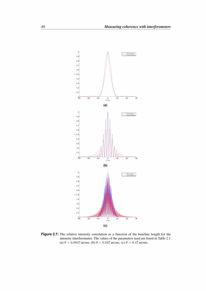
48 Measuring coherence with interferometers
−30 −20 −10 0 10 20 301
1.1
1.2
1.3
1.4
1.5
1.6
1.7
1.8
1.9
2
d [m]
C
GaussianLorentzian
(a)
−30 −20 −10 0 10 20 301
1.1
1.2
1.3
1.4
1.5
1.6
1.7
1.8
1.9
2
d [m]
C
GaussianLorentzian
(b)
−30 −20 −10 0 10 20 301
1.1
1.2
1.3
1.4
1.5
1.6
1.7
1.8
1.9
2
d [m]
C
GaussianLorentzian
(c)
Figure 2.7: The relative intensity correlation as a function of the baseline length for theintensity interferometer. The values of the parameters used are listed in Table 2.1.(a) θ = 0.0047 arcsec, (b) θ = 0.047 arcsec, (c) θ = 0.47 arcsec.

2.4 – Comparison and discussion 49
0 5 10 151
1.1
1.2
1.3
1.4
1.5
1.6
1.7
1.8
1.9
2
d [m]
C
θ = 0.0052"θ = 0.0047"θ = 0.0042"
Figure 2.8: Theoretical correlation values were calculated in order to determine the best fitwith the experimental data. The difference of just a few thousandths of a second ofarc is plainly visible. In this case the angular diameters of θ = 0.0052, 0.0047 and0.0042 arcsec are assumed for a source radiating light with a Gaussian frequencydistribution.
Of course, in real life the correlator will not give pretty readings like those inFig. 2.7. In the very first measurements on Sirius by Hanbury Brown and Twiss in1956 they first calculated the theoretical correlation values for a star radiating like ablack body uniform disk at a typical temperature of its spectral type [12]. The angulardiameter which gave the best fit with the measurements was then equal to the trueangular diameter to within an acceptable uncertainty. As one can see from Fig. 2.8it is fairly easy to discern the difference in the correlation between different angulardiameters down to a few milliseconds of arc.
On the other hand, with the Michelson interferometer it is not as simple as justcounting the minima (which is a point in itself), chiefly due to the presence of twocosine terms with different periods of oscillation, in Eqs. (2.46) and (2.47),
cos(ωτa − kdθ) and cos(ωτa). (2.53)
Rewriting using cτa ≈ dα′ gives
cos[kd(α′ − θ)] and cos(kdα′). (2.54)
It seems that as long as θ is comparable to or smaller than α′, it will not be a very easytask to find θ at all. Looking at Figure 2.9 we see that from (a) to (b) the graph hasa gentle oscillation that does not change much when going from θ = 0.0047 arcsecto θ = 0.047 arcsec, while in (c), with another increase by a factor of 10 to θ = 0.47arcsec, the graph still has its smooth curve, but now with heavy fluctuations. For θ larger

50 Measuring coherence with interferometers
than α′, it should be possible to use the period of the fast oscillation to find the value ofθ. However, already at this preliminary stage we can easily conclude that the intensityinterferometer will more readily allow measurements of much smaller apparent anglesthan the Michelson interferometer will. In all fairness, the value assumed for α′ inTable 2.1 is a ludicrously small number. An angle giving cosα ≈ 10−7 means that theinterferometer is almost precisely normal to the distance vector L of the binary star.Better be careful not to sneeze!
It is time for a recapitulation. The degree of second-order coherence is a measureof the coherence of fluctuations of the intensity of an electric field. Similarly thedegree of first-order coherence is a measure of the coherence of fluctuations of theelectric field amplitude. From Eqs. (2.48) and (2.49) we can glean that it is not actuallythe degree of second-order coherence itself which is the important ingredient in thecorrelation function of the intensity interferometer, but rather the real-valued product ofthe degree of first-order coherences from each source. This is a bit contrary to whatmost textbooks (seemingly) will have one believe, since they more often than not leadup to the intensity interferometer by first introducing g(2)(τ). We also know the relationg(2)(τ) ∼ |g(1)(τ)|2. In a way this is similar to the Poynting vector in that I ∼ |E|2.Following this train of thought, if we take the absolute square of the product of g(1)(τ)from two sources, then another kind of degree of second-order coherence is found, thatquantifies the correlation of the intensities from both sources, i.e.,
〈Ea(t)Ea(t+ τa)Eb(t)Eb(t+ τb)〉 6= 〈Ea(t)Ea(t+ τa)〉〈Eb(t)Eb(t+ τb)〉. (2.55)
The field amplitude correlations are packaged in the intensity correlations, getting rid ofthe troublesome cosω(τa + τb) term. It is this that makes the intensity interferometer alot less of a hassle to work with than the Michelson interferometer.

2.4 – Comparison and discussion 51
−30 −20 −10 0 10 20 300
0.2
0.4
0.6
0.8
1
1.2
1.4
1.6
1.8
2
d [m]
C
GaussianLorentzian
(a)
−30 −20 −10 0 10 20 300
0.2
0.4
0.6
0.8
1
1.2
1.4
1.6
1.8
2
d [m]
C
GaussianLorentzian
(b)
−30 −20 −10 0 10 20 300
0.2
0.4
0.6
0.8
1
1.2
1.4
1.6
1.8
2
d [m]
C
GaussianLorentzian
(c)
Figure 2.9: The relative field correlation as a function of the baseline length for the Michelsoninterferometer. The values of the parameters used are listed in Table 2.1. (a)θ = 0.0047 arcsec, (b) θ = 0.047 arcsec, (c) θ = 0.47 arcsec.


Part II
Coherence in quantum optics
53


Chapter 3
The quantised electric field andquantum coherence
In the previous part the electromagnetic field was treated as a classical field. Theclassical theory is a successful one in the sense that it accounts for a variety of op-tical phenomena, especially those dealing with wave propagation, interference anddiffraction. But a semiclassical theory, in which the field is treated classically whilethe particles are treated by quantum theory, is also able to describe what one couldthink of as purely quantum effects and proof of the existence of photons, such as thephotoelectric effect, Compton-scattering and spontaneous emission [15]. However,there are some effects that can only be accounted for by quantum mechanics, oneof which is known as photon anti-bunching. This discussion is saved for the end ofchapter 4.
The classical degrees of first- and second-order coherence from sections 1.3 and1.4 can be translated to a quantum mechanical coherence theory. But first the freeelectromagnetic field must be quantised using field operators. The density operator willalso be introduced. This is an essential tool in developing the framework to study thequantum correlations of light. Then in section 3.2 the degrees of first- and second-ordercoherence functions will be rewritten in terms of field operators. It will be seen that thedegree of second-order coherence in fact turns out to be a measure of the “classicalness”of light.
Section 3.3 briefly discusses the quantum Hanbury Brown-Twiss effect and howthe intensity interferometer can be interpreted in quantum mechanics. This is followedby section 3.4 where the coherent state is introduced. There it will be concluded thatlight in a coherent state is the closest the quantum mechanical approach can come to aclassical, ideal electric wave.
3.1 Quantisation of the electromagnetic field
Hardly any work on a topic in quantum mechanics can forego mention of the harmonicoscillator, because it is one of few quantum mechanical systems with a simple ex-
55
56 The quantised electric field and quantum coherence
act solution, and any potential can be approximated as a harmonic potential near anequilibrium point. The one-dimensional harmonic oscillator Hamiltonian is
H =p2
2m+
12mω2q2 (3.1)
where m is the mass of a particle subject to a potential V with angular frequency ω,q is the position operator and p is the momentum operator satisfying the canonicalcommutation relation [q, p] = i~.
3.1.1 The ladder-operators of the harmonic oscillator
The reason for bringing up the harmonic oscillator is the very elegant ladder method,due to Paul Dirac, which can be used to solve the eigenvalue problem. This method isalso readily generalized to more complicated problems in quantum field theory. Withoutfurther ado, we introduce the ladder-operators
a = (2~mω)−1/2(mωq + ip)
a† = (2~mω)−1/2(mωq − ip)(3.2)
which are also known as the annihilation and creation operators, respectively. Thesesatisfy the commutation relation
[a, a†] = 1, (3.3)
and the Hamiltonian expressed in terms of a and a† is
H =12
~ω(a†a+ aa†) = ~ω(a†a+12
). (3.4)
It is common to define the number operator
N ≡ a†a (3.5)
such that the eigenvalue of N is the number of photons in the energy eigenstate |n〉
N |n〉 = n |n〉 . (3.6)
The annihilation operator, a, decreases the number of particles in |n〉 by one, while thecreation operator, a†, increases the number by one,
a |n〉 = n1/2 |n− 1〉 , a† |n〉 = (n+ 1)1/2 |n+ 1〉 . (3.7)
The eigenenergy En of state |n〉 is found by applying the Hamilton operator from theleft,
H |n〉 = ~ω(N + 1/2
)|n〉 = En |n〉 (3.8)
The vacuum state is the energy state containing zero particles, |0〉, and can be reachedby applying a from the left. However, there must be a lower limit since the harmonicoscillator should have positive kinetic and potential energies. Thus
a |0〉 = 0. (3.9)

3.1 – Quantisation of the electromagnetic field 57
From Eq. (3.8) the lowest allowed energy E0 is found to be
H |0〉 =12
~ω |0〉 ⇒ E0 =12
~ω. (3.10)
In general the n-photon eigenenergy is
En =(n+
12
)~ω (3.11)
It is useful and quite intuitive to think of the energy eigenvalues as the n photons ofenergy-quanta ~ω. The eigenstates |n〉 are called Fock states or photon number states,and they form a complete set,
∞∑n=0
|n〉 〈n| = 1. (3.12)
From Eq. (3.11) we see that the eigenenergy is discreet and this is the famous contrastto the continuous energy allowed in classical electromagnetism. The state vector is, ingeneral, a superposition of arbitrary Fock states, i.e.,
|ψ〉 =∑n
cn |n〉 (3.13)
where cn are complex coefficients. A special property worth mentioning is that anelectric field in a Fock state contains a precisely determined number of photons, n.There is no uncertainty in this number and so its variation vanishes: (∆n)2 = 0.
3.1.2 The quantised free electric field
When quantizing the electromagnetic field it is customary to work with the vectorpotential A. But the goal here is to rewrite the degrees of first and second-ordercoherence (Eqs. (1.29) and (1.56)), both of which are functions of the electric field.In section 1.1.2 the electric field E(r, t) was prepared as a Fourier expansion with acountable, but infinite number of Fourier coefficients, i.e., the field amplitudes. Thetotal energy of the radiative field was also found and a comparison of Eq. (1.21) toEq. (3.4) suggests the conversion from the classical electric field amplitudes to thequantum mechanical ladder-operators
akλ → akλ and a∗kλ → a†kλ (3.14)
The eigenvector |nk〉 represents the number of photons in mode k. The commutationrelations for the ladder-operators of independent harmonic oscillators k,k′ are [16]
[akλ, ak′λ′ ] = [a†kλ, a†k′λ′ ] = 0,
[akλ, a†k′λ′ ] = δkk′ .
(3.15)
The quantized electric field operator then takes the form
E(r, t) =∑k
∑λ
(~ωk
2ε0L3
)1/2
εkλ
[akλe
i(k·r−ωkt) + a†kλe−i(k·r−ωkt)
]. (3.16)

58 The quantised electric field and quantum coherence
It is common to write the positive and negative frequency parts of the electric fieldoperator separately
E(r, t) = E(+)(r, t) + E(−)(r, t) (3.17)
where
E(+)(r, t) =∑k
∑λ
(~ωk
2ε0L3
)1/2
εkλakλei(k·r−ωkt),
E(−)(r, t) =∑k
∑λ
(~ωk
2ε0L3
)1/2
εkλa†kλe−i(k·r−ωkt).
(3.18)
So E(+)(r, t) contains only the annihilation operators and its adjoint, E(−)(r, t), con-tains only the creation operators.
3.1.3 The density operator
We are now almost ready to rewrite the degree of first and second-order coherence ofsections 1.3 and 1.4, but first a very important tool must be introduced, namely thedensity operator. The approach taken is largely based on that taken in [9], but an evenmore thorough and detailed derivation can be found in [17].
In the optical frequency region, local field measurements can be done by detectorsbased on the photoelectric effect. To put it simply, an atom in its ground state is placedin a radiation field. The electrons kicked out from the atom, often called photoelectrons,are then observed. This measurement is destructive in the sense that the photon isannihilated in the process of producing a photoelectron. Therefore only the annihilationoperator E(+)(r, t) contributes in this process. To simplify things a bit we assume thatthe field is linearly polarized along one direction parallel to the unit vector ε so thatwe can deal with the scalar quantity E(r, t) = ε · E(r, t). In practice this would meanfitting the detector with a polarization filter and only recording the photons parallel toε. The transition probability of the detector atom at position r for absorbing a photonfrom the field is
w(r, t) = |〈f | E(+)(r, t) |i〉|2 (3.19)
where |i〉 is the initial state before the annihilation, i.e., before the detection, and |f〉 isthe final state after annihilation. But the final state is not measured and so we have tosum over all possible final states,
w(r, t) =∑f
|〈f | E(+)(r, t) |i〉|2
=∑f
〈i| E(−)(r, t) |f〉 〈f | E(+)(r, t) |i〉
= 〈i| E(−)(r, t)E(+)(r, t) |i〉 ,
3.1 – Quantisation of the electromagnetic field 59
where the last step is accomplished by using the completeness relation∑f
|f〉 〈f | = 1. (3.20)
Of course, nature being fickle, it is very rare that there is precise knowledge of theinitial state |i〉 of the field; we may know only the probability for the system to be in |i〉.In such a situation one can resort to a statistical description by averaging over all thepossible initial states weighted by their respective probabilities pi
ρ =∑i
pi |i〉 〈i| . (3.21)
This is the density operator and it is a valuable tool when a system is not described bya single state vector, but an ensemble of state vectors |ψ〉1 , |ψ〉2 , . . . , |ψ〉n with aprobability distribution p1, p2, . . . , pn defined over the ensemble. While it is temptingto consider this ensemble to contain both quantum probabilities carried by the statevectors |ψk〉 and classical probabilities carried by the distribution pk, such a sharpdivision may not always be so clear [18].
The density operator satisfies certain properties which are straight forward to show,
hermiticity : ρ† = ρ⇒ pk = p∗k.
positivity : pk ≥ 0 since 〈χ| ρ |χ〉 ≥ 0 ∀ |χ〉.normalization : tr (ρ) = 1⇒∑
k pk = 1.
where tr is short for the trace of an operator, which is the invariant sum of its diagonalmatrix elements for any complete set of states. What is important to note is that allmeasurable information is contained in the density operator, since the expectation valueof any observable can be expressed in terms of ρ,
〈A〉 =∑k
pk 〈ψk| A |ψk〉
=∑k
pk∑i,j
〈ψk |φi〉 〈φi| A |φj〉 〈φj |ψk〉
=∑k
pk∑i,j
〈φj |ψk〉 〈ψk |φi〉 Aij
=∑i,j
ρijAij
= tr (ρA), (3.22)
where the definition of the density matrix has been used:
ρij =∑k
pk 〈φj |ψk〉 〈ψk |φi〉 . (3.23)
So the transition probability can be written as
w(r, t) =∑i
pi 〈i| E(−)(r, t)E(+)(r, t) |i〉
= tr [ρE(−)(r, t)E(+)(r, t)] (3.24)

60 The quantised electric field and quantum coherence
3.2 The quantum mechanical degrees of first- and second-order coherence
In section 1.3 the classical first-order correlation function was defined as the long-time1
average of the electric wave radiated from a single source. Then the ergodic natureof chaotic light was used to equal the time-average to the statistical average of anensemble of identical atoms. If the radiation fields are wide-sense stationary, (i.e., thecorrelation functions are independent of time), then the correlation only depends on thetime difference τ = t2 − t1 between two measurements of the field at the same point rin space. This leads to the definition of the quantum mechanical first-order correlationfunction of the electric field
〈E(−)(r, t)E(+)(r, t+ τ)〉 = tr [ρE(−)(r, t)E(+)(r, t+ τ)]. (3.25)
Note that the field operators are in normal order; The annihilation operators are to theright of all the creation operators in each product of operators. The advantage of normalordering is that the expectation value of any normal product vanishes. We are free towrite any observable in normal order since this merely corresponds to changing theparticular order of factors (which are c-numbers) before quantization of the field [19].For example, the average intensity at point r at time t is
〈I(r, t)〉 = 〈E(−)(r, t)E(+)(r, t)〉, (3.26)
and the observable intensity-intensity correlation function is not 〈I(r, t)I(r, t)〉, butrather the normally ordered product
〈NI(r, t)I(r, t)〉 = 〈E(−)(r, t)E(−)(r, t)E(+)(r, t)E(+)(r, t)〉, (3.27)
where N denotes the normal product.
In a similar way as for Eq. (3.25) we define the quantum mechanical second-ordercorrelation function of the electric field
〈E(−)(r, t)E(−)(r, t+ τ)E(+)(r, t+ τ)E(+)(r, t)〉= tr [ρE(−)(r, t)E(−)(r, t+ τ)E(+)(r, t+ τ)E(+)(r, t)]. (3.28)
Thus the normalised quantum mechanical degree of first-order coherence for awide-sense stationary field is
g(1)(τ) =〈E(−)(t)E(+)(t+ τ)〉〈E(−)(t)E(+)(t)〉
(3.29)
and the normalised quantum mechanical degree of second-order coherence
g(2)(τ) =〈E(−)(t)E(−)(t+ τ)E(+)(t+ τ)E(+)(t)〉
〈E(−)(t)E(+)(t)〉2(3.30)
1Long-time as in much longer than the coherence time of the light.

3.2 – The quantum degrees of first- and second-order coherence 61
Note that in the definition of g(2)(τ) the operators have also been time ordered. Timeordering is defined as
T φ(x)φ(x′) =
φ(x)φ(x′), t > t′
φ(x′)φ(x), t′ > t(3.31)
where t = x/c etc. The effect is that the earliest operator acts on the state first.Specifically the creation operator in E(−)(t) will act leftwards on the bra first, followedby E(−)(t+ τ), while the annihilation operator in E(+)(t) acts to the right on the ket,before E(+)(t+ τ).
Remember that we are still dealing with the scalar frequency parts of the electricfields and do not have to worry about the polarisation. Also keep in mind that sincewe are focussing only on temporal coherence, it is purposeful to keep the notation assimple as possible by only explicitly writing the time dependence of the degrees ofcoherence. The spatial dependence can always be reintroduced via
τ = t2 − t1 − (|r2| − |r1|)/c. (3.32)
3.2.1 In the limits of quantum coherence
The quantum degree of first-order coherence does not lead to any conflict with theclassical limits defined in Eq. (1.32), which is equivalent to saying that it does notexhibit any signature of field quantisation. For a single-mode electric field, g(1)(τ) isgreatly simplified as most of the factors cancel out and we are left with simply
g(1)(τ) =〈a†a〉eiωτ〈a†a〉 = eiωτ . (3.33)
This is in accordance with the classical result in Eq. (1.34) and shows that any planeparallel single-mode light beam is first-order coherent for all pairs of space-time points.
Since the numerator in Eq. (3.30) is the expectation value of an operator multipliedwith its Hermitian conjugate, it must be positive [1] and it follows that
0 ≤ g(2)(τ) ≤ ∞, (3.34)
which is similar to the range of the classical degree of second-order coherence. Howeverit is not possible to show that the quantum g(2)(τ) satisfies either of the inequalitiesEq. (1.63) or Eq. (1.67).
The degree of second-order coherence also simplifies for a single-mode field to
g(2)(τ) =〈a†a†aa〉〈a†a〉2 =
〈(a†a)2〉 − 〈a†a〉〈a†a〉2
=〈N2〉 − 〈N〉〈N〉2 = 1 +
(∆N)2 − 〈N〉〈N〉2 (3.35)

62 The quantised electric field and quantum coherence
where we use the definition of the number operator and the commutator of the ladder-operators. The variance in the photon number cannot be negative, so
(∆N)2 ≡ 〈N2〉 − 〈N〉2 ≥ 0. (3.36)
Inserting this into g(2)(τ) we see that any single-mode field must satisfy the inequality
g(2)(τ) ≥
1− 1〈N〉 for 〈N〉 ≥ 1
0 for 〈N〉 < 1.(3.37)
This limit is independent of space and time, but it does depend on the nature of thelight, since the variance in photon number (∆N)2 is not the same for the differenttypes of light. Clearly g(2)(0) violates the classical lower limit Eq. (1.63). Light withdegree of second-order coherence outside of the classical range (∈ [1,∞]) must then beconsidered to be non-classical. This topic is discussed in more detail in section 4.5.1.
3.3 The Quantum Hanbury Brown-Twiss effect
In section 2.3 we used classical electric fields to demonstrate that the intensity interfer-ometer measures the degree of second-order coherence, g(2)(τ). We then saw that theHanbury Brown-Twiss effect gives an enhanced relative intensity correlation betweenchaotic light beams incident on two photodetectors, an effect not seen for coherentsources.
Hanbury Brown and Twiss originally proposed a radio intensity interferometerto measure the angular diameter of radio stars. This was widely accepted by bothradio engineers and physicists since at the wavelengths where radio astronomy isapplied, classical electromagnetism is considered to give a sufficient description of theinterference effect. However, when they ventured to apply the intensity interferometerto optical wavelengths they were met with outright scepticism and charges of it being apatently absurd idea.
Since the classical derivation has been given much attention it adds a certaincompleteness to devote a few paragraphs to the quantum approach. We will not go intoa detailed derivation but will briefly mention the criticism of the intensity interferometerand how coincidence counting of photons led to the discovery of photon bunching andits relation to the degree of second-order coherence.
3.3.1 Trouble in Hilbert space
The problem with applying the intensity interferometer on light, it was thought, wasthat at optical wavelengths the energies would require the light to be quantised in arelatively small number of photons. It would then not be correct to use Maxwell’sequations on light waves and only introduce quantisation through the discrete energylevels in the photodetectors. What was more, if one instead thought of the light in terms

3.3 – The Quantum Hanbury Brown-Twiss effect 63
of photons, the enhanced intensity correlation would imply that the photon’s arrivalat the two separated detectors would be correlated. Somehow, the photons from twoincoherent sources would then “know” that they should arrive at a detector at the sametime, in “clumps”.
Obviously, in order for the interference to take place there has to be several differentphotons incident on the detectors at the same time. A quite worrisome requirementsince P. Dirac stated that 2
“[A] photon [...] interferes only with itself. Interference between twodifferent photons never occurs.”
In order to avoid violation of this dictum one needs to do some mental gymnastics.There are at the least two possible ways to think about this. For example, one can evadethe dictum by saying that in a two-photon state there is no way to determine which atomemitted or absorbed which photon [20]. Or, one can think of each emitting atom to becoupled to a mode in a universal radiation field, so that a photon is simply a particularenergy eigenstate of one such radiation mode [21].
This was not the only objection raised. Hanbury Brown and Twiss also had to fendoff complaints of violation of the uncertainty relation3 and of the laws of thermodynam-ics4. Lastly there were performed a few laboratory experiments that claimed to disprovethe correlation of photons at two separate detectors, most notably the experiment byBrannen and Ferguson5 which concluded that
“[No] correlation [...] exists between photons in coherent light rays”,and that“[If] such a correlation did exist, it would call for a major revision of somefundamental concepts in quantum mechanics”.
These conclusions were quickly shot down as it turned out that the sensitivity of theequipment being used was so low that an observation period of a 1000 years would benecessary in order to see any correlations [22].
In Hanbury Browns own words the remonstrations against the intensity interferom-eter originated from “[Troubled] physicists who had been brought up on particles andhad not fully appreciated that the concept of a photon is not a complete picture of light”[7]. In the end Hanbury Brown and Twiss were vindicated, and have since been grantedthe honour of laying the experimental foundation for contemporary quantum optics andfor providing new methods for fundamental tests of quantum mechanics [20].
2Dirac, P.A.M., The Principles of Quantum Mechanics, Oxford Clarendon Press, 4th ed, 19893 A point refuted by the fact that the intensity interferometer measures only the relative phase between
the two light beams. The total energy and the relative phase can be represented by commuting operatorsand can incidentally be described by classical theory.
4 The correction lies in taking into account that the total total fluctuations in the temperature of thebody must be treated as due to interaction between incident, emitted and reflected streams of radiation.
5 Brannen, E. and Ferguson, H.I.S., Nature, 178, 481 (1956).

64 The quantised electric field and quantum coherence
Figure 3.1: The two indistinguishable events where (solid arrows) a emits a photon detectedby c and b emits one detected by d, and (dashed arrows) a emits a photon detectedby d and b emits one detected by c.
3.3.2 The essence of the quantum interpretation
Consider two source atoms a and b initially in excited states without any phase cor-relation. They both emit photons which are absorbed by the “detector” atoms c andd. There are basically four different events that will lead to excitations of c and d ifone assumes that each detector can only be excited by one photon at a time [23]: (i)Atom a can emit two photons that are detected at c and d, respectively, and (ii) b canemit two photons that are detected at c and d. These processes are distinguishable anddoes not lead to any interference. (iii) Atom a can emit a photon detected at c, with bemitting a photon detected in d. (iv) Atom a can emit a photon detected at d, with bemitting a photon detected in c, see Fig. 3.1. It is not possible to tell events (iii) and (iv)apart since photons are indistinguishable particles. Thus the system state vector is asuperposition of (iii) and (iv)
|c, d〉 =1√2
[|a→ c, b→ d〉+ |b→ c, a→ d〉
](3.38)
and this is the origin of the correlation seen in the quantum Hanbury Brown-Twisseffect.
The probability that c is excited when in the presence of sources a and b is the sumof the probabilities that c is excited by a without b present and by b without a present
Pc = P (a→ c) + P (b→ c). (3.39)
Likewise the probability that d is excited, Pd. By the argument of Fano [24] theprobability of excitation of both c and d, Pc,d, is not just equal to the product PcPd,nor can it be simply expressed as a function of the probabilities P (a→ c), P (b→ c),P (a→ d) or P (b→ d). Instead Pc,d is an oscillatory function of the distance betweenc and d, provided the two excitations are close enough in time. This result is in completeagreement with what we found from the classical description in section 2.3.
The probability distribution of an excitation over time is equivalent to a countingdistribution of n photons detected, so we make a switch in variables. We define acoincidence as detections of a photon at c and d simultaneously, where “simultaneous”in practical terms means within some short time τ according to the resolution time of

3.4 – Coherent states of the electric field 65
the setup. If the counter N registers a coincidence when two photons arrive at c, d, theaverage coincidence rate is
N = 2NcNdτ [1 + 1/2|g(1)(0)|2], (3.40)
where Nc(d) is the average counting rate of photons arriving at c(d) [7]. This resultis valid for a resolving time much shorter than the coherence time (which is inverselyproportional to the angular frequency). So if the light is not first-order coherent, thenthe coincidence rate is simply the expected rate for two uncorrelated streams of photons2NcNdτc. But if the light is at least partially first-order coherent (|g(1)(0)| > 0), thereis an excess in the coincidence rate which varies directly with the degree of first-ordercoherence, i.e., the photons tend to arrive in “clumps”. Recall that classical chaotic lightis partially first-order coherent for small τ (see Fig. 1.2). This is the quantum HanburyBrown and Twiss effect. Of course the “clumping” is not unique to photons, but appliesgenerally to bosons. Where bosons are social animals, fermions have antisymmetricwavefunctions which manifests as an “anti-clumping”. This “clumping” is discussedmore in section 4.5.2 where it will be given a more contemporary name.
As a comment to Eq. (3.38) it does make sense that photons detected within a timeinterval shorter than their coherence time τc ∼ 1/∆ω can be regarded as occupying thesame state. Due to the Heisenberg uncertainty principle the uncertainty in energy mustbe on the order of ~∆ω ∼ ~/τc, and the uncertainty in arrival time is similarly 1/∆ω.These two quantities define a unit cell in phase space, which the resolution time τ τcis well within [25].
3.4 Coherent states of the electric field
Coherent states were first discovered by E. Schrödinger (1926) as states of the harmonicoscillator with a minimum uncertainty product. These minimum-uncertainty states didnot attract much attention until R. J. Glauber (1963) used them to develop a completequantum mechanical description of the photon statistics of arbitrary radiation fields.The states were renamed coherent states by Glauber, but are also referred to by others asGlauber states. The work was inspired by the then relatively heated debate regarding theresults of the optical intensity interferometer and it culminated in a complete quantummechanical coherence theory to the Nth order.
Up until then nearly all quantum electrodynamical calculations had been carriedout through the use of the Fock states, which are purely quantum mechanical states inthe sense that they have no equivalence to any known classical fields. In practice thislimited the calculations to only dealing with a few photons at a time, while in optics it isoften the case that the number of photons is large and not necessarily precisely known.Glauber found that the coherent states, which are closely related to the coherenceproperties of fields, have the ability to represent the classical limit of a field and stillpreserve the quantum mechanical aspects of it [16, 26].
The coherent state is the eigenstate of the annihilation operator introduced insection 3.1. As a is not Hermitian we must allow for it to have a complex eigenvalue,
a |α〉 = α |α〉 , (3.41)
66 The quantised electric field and quantum coherence
with the corresponding bra-state
〈α| a† = α∗ 〈α| . (3.42)
The coherent state can be expanded in a linear superposition of the Fock states
|α〉 = e−|α|2/2
∞∑n=0
αn√n!|n〉 (3.43)
which is clearly seen to be normalised
〈α |α〉 = e−|α|2∞∑n=0
|α|2nn!〈n |n〉 = 1. (3.44)
Furthermore, the coherent-state expectation value for the number operator is
〈n〉 = 〈α| n |α〉 = 〈α| a†a |α〉 = |α|2 (3.45)
and similarly for the second moment
〈n2〉 = 〈α| n2 |α〉 = 〈α| a†a†aa |α〉 = 〈α| a†aa†a |α〉+ 〈α| a†a |α〉= |α|4 + |α|2
From this we find the variance of the photon number
(∆n)2 = 〈n2〉 − 〈n〉2 = |α|2 (3.46)
So the relative variance, or uncertainty, in the number of photons in a coherent statedecreases when the amplitude of the coherent state increases,
∆n〈n〉 =
1|α| =
1√〈n〉
. (3.47)
The classical analogy of a vanishing variance in photon number is an ideal wavewith no intensity fluctuations, which can be called stable. So the fact that the variance isnon-vanishing can be interpreted as an aspect of the particle nature of light in quantummechanics. However, the importance of this aspect diminishes with increase in the meanphoton number 〈n〉. This can be viewed as a manifestation of Bohr’s correspondenceprinciple; As the number of photons increases, the coherent state becomes more andmore classical, with smaller and smaller relative fluctuations in energy.
The quantised electromagnetic field can be in a coherent state, obtainable by spec-ifying a coherent state for each of the modes k of the field. Each mode of the fieldcorresponds to a single, isolated harmonic oscillator so the multi-mode coherent statevector is the product form
|α〉 ≡ |αk1 , αk2 , . . . , αkn〉 = |αk1〉 ⊗ |αk2〉 ⊗ · · · ⊗ |αkn〉 (3.48)

3.4 – Coherent states of the electric field 67
The electric field operator E(r, t) has a particularly simple expectation value when thefield is in a coherent state,
〈E(r, t)〉 = 〈α| E(r, t) |α〉
=∑kλ
(~ωk
2ε0L3
)1/2
εkλ[αkλe
i(k·r−ωkt) + α∗kλe−i(k·r−ωkt)
](3.49)
This is on the same form as the mode expansion of the corresponding classical fieldEq. (1.18), where αkλ represents the well-defined complex amplitude of the classicalfield mode k. Note, however, that despite this similarity, Eq. (3.49) is merely theaverage field in the coherent state and being a quantised field it also exhibits quantumfluctuations, whereas a coherent classical electric field will not show fluctuations inneither amplitude nor phase. In addition, the variance of the field vector does not vanishevent though the expectation values (the first and second moment) resembles that of aclassical field of well-defined complex amplitude αkλ.
So, quantum fluctuations being a fact of life, the coherent state can be shown to bea quadrature minimum-uncertainty state for all mean photon numbers 〈n〉 = |α|2. Ifthe annihilation and creation operators are expanded as
a = X1 + iX2 and a† = X1 − iX2 (3.50)
where X1 and X2 are dimensionless quadrature operators6, a little algebra yields theexpectation values of the quadrature operators
〈X1〉 =12〈α| a† + a |α〉 =
12
(α∗ + α) (3.51)
and
〈X2〉 =i
2〈α| a† − a |α〉 =
i
2(α∗ − α). (3.52)
The expectation values of the squares of the quadrature operators are found by employ-ing the commutation identity of the ladder-operators
X21 =
14
[a† + a]2 =14
[a†a† + aa+ 2a†a+ 1] (3.53)
giving
〈X21 〉 =
14
[(α∗)2 + α2 + 2|α|2 + 1]. (3.54)
Similarly
〈X22 〉 =
14
[−(α∗)2 − α2 + 2|α|2 + 1]. (3.55)
6 The quadrature operators can be recognised as dimensionless forms of the quantum mechanicalposition and momentum operators, q and p respectively.

68 The quantised electric field and quantum coherence
The quadrature variances are then7
(∆X1)2 = (∆X2)2 =14
(3.56)
which are independent of the photon number. Furthermore, the uncertainty relation isthe equality
(∆X1)(∆X2) =14
(3.57)
Thus for any mean photon number the coherent state is a quadrature minimum-uncertainty state. This also includes the vacuum state where α = 0, meaning thatall coherent states have the same uncertainty as vacuum. Thus one can interpret the“fuzziness” of the coherent state as being due to vacuum fluctuations. It may be saidthat the minimum uncertainty represents an incoherent part of the quantised field whichis a result of quantum fluctuations. Hence the energy of the total quantised field will bea sum of this vacuum energy and the fields coherent energy [27]. This is in contrast tothe classical coherent light which, as mentioned several times now, does not fluctuateand will have no energy addition from the vacuum since the classical vacuum energy iszero. In section 2.3.3 we discussed a phenomena called shot noise that is observed inoptical detection (specifically in the intensity interferometer) and its origin is thoughtto be exactly this quantum uncertainty in light, namely the ever present vacuum fieldmodes [3].
A phase diagram for the coherent state |α〉 can be drawn if α is separated into itsamplitude and phase by
α = |α|eiφ (3.58)
where θ is the mean phase of the coherent-state excitation of the field mode, such that
X1 = |α| cosφ, X2 = |α| sinφ. (3.59)
|α〉 can be considered a displaced vacuum state where the uncertainty “cloud” is shiftedfrom the origin by the quadrature vector of length |α| at an angle φ to the X1-axis [3],see Fig. 3.2. The diameter of the shaded circle at the end of |α| is ∆X1 = ∆X2 = 1/2.By geometric means, the variance of the phase, ∆φ, can be deduced from the diagram,
tan ∆φ/2 =1/22|α| (3.60)
The evaluation of the uncertainty in the phase φ, however, is not straight forward sincea phase eigenstate or a phase operator cannot be represented within the usual infiniteHilbert space [28]. Instead we can derive a number-phase uncertainty relationship basedon geometrical arguments rather than commutation relations between number and phaseoperators. This result will correctly represent a trade-off between the values of the
7 Note that the coherent state is a special case of a squeezed state since the quadrature variances areequal, which they need not always be.
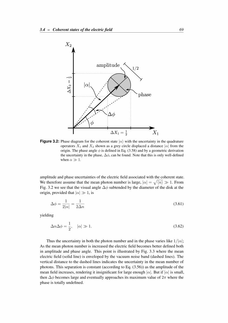
3.4 – Coherent states of the electric field 69
Figure 3.2: Phase diagram for the coherent state |α〉 with the uncertainty in the quadratureoperators X1 and X2 shown as a grey circle displaced a distance |α| from theorigin. The phase angle φ is defined in Eq. (3.58) and by a geometric derivationthe uncertainty in the phase, ∆φ, can be found. Note that this is only well-definedwhen α 1.
amplitude and phase uncertainties of the electric field associated with the coherent state.We therefore assume that the mean photon number is large, |α| =
√〈n〉 1. From
Fig. 3.2 we see that the visual angle ∆φ subtended by the diameter of the disk at theorigin, provided that |α| 1, is
∆φ =1
2|α| =1
2∆n(3.61)
yielding
∆n∆φ =12, |α| 1. (3.62)
Thus the uncertainty in both the photon number and in the phase varies like 1/|α|;As the mean photon number is increased the electric field becomes better defined bothin amplitude and phase angle. This point is illustrated by Fig. 3.3 where the meanelectric field (solid line) is enveloped by the vacuum noise band (dashed lines). Thevertical distance to the dashed lines indicates the uncertainty in the mean number ofphotons. This separation is constant (according to Eq. (3.56)) as the amplitude of themean field increases, rendering it insignificant for large enough |α|. But if |α| is small,then ∆φ becomes large and eventually approaches its maximum value of 2π where thephase is totally undefined.

70 The quantised electric field and quantum coherence
Π 2 Π
Figure 3.3: One period of the electric field in a single-mode coherent state where the dashedlines indicate the uncertainty in phase and amplitude due to quantum fluctuations.Adapted from [1].
In contrast to the coherent state, the Fock number state has a sharply defined photonnumber. By the same line of reasoning as above, the Fock state must then have amaximal uncertainty in the phase, that is φ ∈ [0, 2π]. The energy eigenvalue relationcan be written in terms of the quadrature operators as
~ω(a†a+ 1/2) |n〉 = ~ω(X21 + X2
2 ) |n〉 = ~ω(n+ 1/2) |n〉 (3.63)
resulting in the variances
(∆X1)2 = (∆X2)2 =12
(n+ 1/2) (3.64)
Thus the vacuum state is the quadrature minimum-uncertainty state. Fig. 3.4 illustratesthe quadrature properties of the Fock state. The phase of the quadrature operators ismaximally uncertain, so the radius of the circle spanned by X1 + X2 is found fromEq. (3.63),
3.5 Summary and discussion
In this chapter we have quantised the electric field and introduced the ladder-operatorsof the harmonic oscillator. The coherent states are the eigenstates of these operatorsand they offer very convenient calculations of the electric field near the classical limit.This is seen by both the fact that we can recognize their eigenvalues as the complexamplitude of the classic field, but also because they are minimum uncertainty states,which was shown in section 3.4. There we saw that while light in a coherent state is bynature quantum mechanical in that it exhibits quantum fluctuations, this aspect growsless and less important for higher eigenvalues (i.e., higher photon number).

3.5 – Summary and discussion 71
Figure 3.4: Phase-diagram for the Fock state |n〉, with sharply defined photon number in thequadrature operators, but maximal uncertainty in the phase.
Although the expectation value of the electric field in a coherent state is non-zerowith a classical-looking form, as opposed to the vanishing value of a Fock state, thisis not exactly equal to the classical field. One can instead think of the quantised fieldas being comprised of two components: the classical field plus a part containing thequantum features, such as the vacuum fluctuation. In conclusion we can declare coherentstates to come as close as possible to being classical states of definite complex amplitude.In particular coherent states are especially suited for describing electromagnetic fieldsgenerated from so-called coherent sources, lasers being one of them.
The density operator was also introduced. This is an invaluable tool when we lackthe full information of a quantum system since it provides a statistical description of itinstead. The density operator was used in section 3.2 to derive the quantum mechanicaldegrees of first- and second-order coherence, but the last of ρ has not been seen yet: Inchapter 5 it is critical in the quantum mechanical description of the laser. But beforedelving into the properties of the laser the first stop is chapter 4 which investigateshow the quantum degrees of first- and second-order coherence differs for light in threedifferent states; the coherent state, the Fock state and the mixed thermal state. Theresults are used to define some categories pertaining to the statistical properties of thephotons. This discussion will show that the mechanism behind the quantum HanburyBrown-Twiss effect, briefly mentioned in section 3.3, is related to the quantum g(2)(τ).

Chapter 4
Calculations of the quantumdegrees of coherence
The previous chapter introduced the necessary background for investigating the coher-ence properties of radiation fields. We will now calculate the quantum degrees of first-and second- order coherence for light in three different states, in order of appearance,
- The coherent state
- The Fock state
- The mixed thermal state
For all three, g(1)(τ) and g(2)(τ) will be calculated both for single-mode light and formulti-mode light1.
The quantum Hanbury Brown-Twiss effect was in section 3.3 described as a “clump-ing” of photons. A more contemporary name is photon bunching and a discussion ofthis and the relation to g(2)(τ) is covered in section 4.5. There we will also touch uponthe photon number statistics of the aforementioned states of light.
4.1 Light in a coherent state
4.1.1 Single-mode photon field
For a single-mode photon field in a coherent state |α〉 the degree of first-order coherenceis
g(1)(τ) =〈a†k ak〉eiωkτ
〈a†k ak〉=〈α| a†k ak |α〉 eiωkτ
〈α| a†k ak |α〉= eiωkτ (4.1)
1Some textbooks (e.g., [1]) prefer to calculate multi-mode fields as the simpler continuous-mode.
73

74 Calculations of the quantum degrees of coherence
which is a trivial result similar to what was found in the classical case in section 1.3 andit affirms that light in a coherent state is first-degree coherent for all pairs of space-timepoints.
The degree of second-order coherence is
g(2)(τ) =〈a†k a
†k ak ak〉
〈a†k ak〉2=〈α| a†k a
†k ak ak |α〉
〈α| a†k ak |α〉2
=(α∗)2α2
(α∗α)2= 1. (4.2)
Again the result is equal to that for the classical ideal wave Eq. (1.69) and it satisfiesthe requirement Eq. (1.70) as |g(1)(τ)| = g(2)(τ) = 1. Thus, single-mode light in acoherent state is second-order coherent. So far we can deduce that in fact the coherentstate is the quantum analogue of classical coherent light.
4.1.2 Multi-mode photon field
If the photon field is instead a multi-mode field, the state vector is a product state of thedifferent k modes
|α〉 =∏k
⊗ |αk〉 = |αk1〉 ⊗ |αk2〉 ⊗ · · · ⊗ |nkν 〉 . (4.3)
Here α denotes the complete set of complex amplitudes that specify the coherentstates in each excited mode in the cavity, i.e., each photon present in the radiation field.This gives the degree of first-order coherence as
g(1)(τ) =
∑k1,2
√ωk1ωk2〈a†k1
ak2〉ei[(k2−k1)·r−(ωk2−ωk1 )t]eiωk2τ
∑k1,2
√ωk1ωk2〈a†k1
ak2〉ei[(k2−k1)·r−(ωk2−ωk1 )t]
=
∑k1,2
√ωk1ωk2 〈α| a†k1
ak2 |α〉 ei[(k2−k1)·r−(ωk2−ωk1 )t]eiωk2τ
∑k1,2
√ωk1ωk2 〈α| a†k1
ak2 |α〉 ei[(k2−k1)·r−(ωk2−ωk1 )t]
=
∑k1,2
√ωk1ωk2α
∗k1αk2e
i[(k2−k1)·r−(ωk2−ωk1 )t]eiωk2τ
∑k1,2
√ωk1ωk2α
∗k1αk2e
i[(k2−k1)·r−(ωk2−ωk1 )t]
=
∑k
√ωkαke
i(k·r−ωkt)eiωkτ∑k
√ωkαke
i(k·r−ωkt)(4.4)
an expression which is identical to the classical g(1)(τ) for a multi-mode electric field ifone identifies the coherent state eigenvalue α with the classical complex field amplitude

4.1 – Light in a coherent state 75
a. This is in agreement with the multi-mode coherent state being an eigenstate of thepositive frequency part of the electric field operator
E(+)(r, t) |α〉 =∑k
(~ωk
2ε0L3
)1/2
αkei(k·r−ωkt) |α〉 (4.5)
The degree of first-order coherence is now a normalised sum of the classical electric fieldof each mode, modulated by the observation delay τ . Note that
∑k1,2
is a understoodto be a multiple sum over different modes, i.e.,
∑k1k2
. Remember that according tothe Wiener-Khinchin theorem g(2)(τ) is a Fourier pair with the power spectral densityof the light (see section 1.3.2). In the case of the single-mode field S(ω) is the Deltafunction implying a zero line width of the frequency distribution, as expected. On theother hand, a multi-mode field should have a spread in the k-room.
An analogous calculation yields the following expression for g(2)(τ)
g(2)(τ) =
∑k1,2,3,4
√ωk1ωk2ωk3ωk4〈a†k1
a†k2ak3 ak4〉[∑
k1,2
√ωk1ωk2〈a†k1
ak2〉ei[(k2−k1)·r−(ωk2−ωk1 )t]
]2
× ei[(k4+k3−k2−k1)·r−(ωk4+ωk3−ωk2−ωk1 )t]ei(ωk3−ωk2 )τ
=
∑k1,2,3,4
√ωk1ωk2ωk3ωk4α
∗k1α∗k2
αk3αk4[∑k1,2
√ωk1ωk2α
∗k1αk2e
i[(k2−k1)·r−(ωk2−ωk1 )t]
]2
× ei[(k4+k3−k2−k1)·r−(ωk4+ωk3−ωk2−ωk1 )t]ei(ωk3−ωk2 )τ
=
∑k1,2
√ωk1ωk2α
∗k1αk2e
i[(k2−k1)·r−(ωk2−ωk1 )t]ei(ωk2−ωk1 )τ
∑k1,2
√ωk1ωk2α
∗k1αk2e
i[(k2−k1)·r−(ωk2−ωk1 )t]
= |g(1)(τ)|2 (4.6)
Again, this is similar to the classical expression for the degree of second-order coherenceof multi-mode light and it is proportional to the degree of first-order coherence. Workingwith multi-mode light muddies the waters a bit, but we see that this result is on the sameform as for single-mode light, since
g(2)(τ)single = |g(1)(τ)single|2 = 1 (4.7)
Without knowing how |g(1)(τ)| is affected by there being multiple modes, the degree ofsecond-order coherence is still on the same form
g(2)(τ)multi = |g(1)(τ)multi|2. (4.8)

76 Calculations of the quantum degrees of coherence
4.2 Light in a Fock state
4.2.1 Single-mode photon field
For a single-mode photon field we find the degree of first-order coherence to be
g(1)(τ) =〈a†k ak〉eiωkτ
〈a†k ak〉=〈n| a†k ak |n〉 eiωkτ
〈n| a†k ak |n〉= eiωkτ (4.9)
The above gives the same first-order coherence as for a photon field in a coherent state,leading us to conclude that light in a Fock state is first-order coherent at all pairs ofspace-time points.
Carrying on, the degree of second-order coherence is
g(2)(τ) =〈a†k a
†k ak ak〉
〈a†k ak〉2=〈nk| a†k a
†k ak ak |nk〉
〈nk| a†k ak |nk〉2=〈n2
k〉+ nk
n2k
(4.10)
where the mean photon number is 〈nk〉 ≡ nk. We define the variance in the photonnumber nk as
(∆nk)2 = 〈n2k〉 − 〈nk〉2, (4.11)
But the Fock state is the eigenstate of the number operator where the eigenvalue is themean number of photons in mode k. So the expectation value of the photon number hasno uncertainty in it, and therefore there is no variance in the photon number, ∆nk = 0,
g(2)(τ) = 1 +(∆nk)2
nk2− 1nk
=
1− 1nk
for nk ≥ 1
0 for nk < 1(4.12)
which is in agreement with Eq. (3.34). But, since we cannot show that g(2)(τ) > 1 likewe can for the classical degree of second order coherence, so there will be an intervalwhere
0 ≤ g(2)(τ) ≤ 1 (4.13)
which is non-classical in the sense that there are no equivalent classical field with sucha value of the second-order coherence. Although g(2)(τ) does not strictly depend on τwe will stick to this notation for cohesion with the instances where the time-dependencydoes exist.
Looking back at Eq. (4.9) it could be a little puzzling that what we call the quantumanalogue of classical light has the same g(1)(τ) as the light we just concluded must beentirely non-classical. We will soon see that light in a mixed thermal state also hasthe same g(1)(τ) for single-mode light. This is the reason it has been claimed that it isg(2)(τ) that can distinguish between the nature of different types of light. In fact, anysingle-mode light will be first-order coherent.

4.2 – Light in a Fock state 77
4.2.2 Multi-mode photon field
As with the coherent product state we use a short notation for a multi-mode Fock-state
|n〉 =∏k
⊗ |nk〉 = |nk1〉 ⊗ |nk2〉 ⊗ · · · ⊗ |nkν〉 . (4.14)
where there is no correlation between the different modes ki, (i = 1, 2, . . . , ν). Inthis setting the meaning of “uncorrelated” relates to the lack of entanglement betweenphoton states of different modes, where entanglement is a purely quantum mechanicalphenomenon.
The orthonormality of the number states ensures that the expectation value of anoperator consisting of a† and a is zero, unless they appear in equal number of the samemode ki,∑
k1,2
〈a†k1ak2〉 =
∑k1,2
〈nk1 | 〈nk2 | a†k1ak2 |nk1〉 |nk2〉
=
∑k1,2
〈a†k1〉〈ak2〉 = 0 for uncorrelated modes
∑k
〈a†k ak〉 =∑k
nk for correlated modes k1 = k2
(4.15)
Then g(1)(τ) is
g(1)(τ) =
∑k1,2
〈a†k1ak2〉√ωk1ωk2e
i[(k2−k1)·r−(ωk2−ωk1 )t]eiωk2τ
∑k1,2
〈a†k1ak2〉√ωk1ωk2e
i[(k2−k1)·r−(ωk2−ωk1 )t]
=
∑k1,2
〈n| a†k1ak2 |n〉
√ωk1ωk2e
i[(k2−k1)·r−(ωk2−ωk1 )t]eiωk2τ
∑k1,2
〈nk| a†k1ak2 |nk〉
√ωk1ωk2e
i[(k2−k1)·r−(ωk2−ωk1 )t]
=
∑k
nkωkeiωkτ
∑k
nkωk(4.16)
since 〈n| a†k1ak2 |n〉 = δk1,k2 . As expected the degree of first-order coherence
now reflects the presence of many modes in the light2.2A possible way to proceed could be to assume that the light is emitted in wave-packet of a Gaussian
form, like in [1]. This would yield a g(2)(τ) that is identical to that of the single-mode field.

78 Calculations of the quantum degrees of coherence
An analogous calculation yields the following expression for the degree of second-order coherence
g(2)(τ) =
∑k1,2,3,4
〈a†k1a†k2
ak3 ak4〉√ωk1ωk2ωk13ωk4[∑
k1,2
〈a†k1ak2〉ei[(k2−k1)·r−(ωk2−ωk1 )t]
]2
× ei[(k4+k3−k2−k1)·r−(ωk4+ωk3−ωk2−ωk1 )t]ei(ωk3−ωk2 )τ
Before we proceed we observe that the modes k1,2,3,4 can come in the followingcombinations
1 6= 2 6= 3 6= 4 → 〈a†k1a†k2
ak3 ak4〉ei(ωk3−ωk2 )τ = 0
1 = 2 6= 3 = 4 → 〈a†k1a†k1
ak3 ak3〉ei(ωk3−ωk1 )τ = 0
1 = 3 6= 2 = 4 → 〈a†k1a†k2
ak1 ak2〉ei(ωk1−ωk2 )τ = nk1nk2ei(ωk1−ωk2 )τ
1 = 4 6= 2 = 3 → 〈a†k1a†k2
ak2 ak1〉ei(ωk2−ωk2 )τ = nk1nk2
1 = 2 = 3 = 4 → 〈a†k a†k ak ak〉ei(ωk−ωk)τ = nk(nk − 1)
Continuing with g(2)(τ) we have
g(2)(τ) =
∑k1,2
nk1nk2ωk1ωk2ei(ωk1−ωk2 )τ −
∑k
nkω2k1∑
k1,2
nk1nk2ωk1ωk2
= |g(1)(τ)|2 −∑
k nkω2k[∑
k nkωk]2 (4.17)
This is on a similar form as that for single-mode
g(2)(τ)single = 1− 1nk
with
g(2)(τ)multi = 1− 1n
(4.18)
if n is the weighted number of photons of all the populated modes. Consistent withthe single-mode result, the degree of second-order coherence is less than the lowestclassical limit of g(2)(τ)cl ≥ 1, and thus in the non-classical range [0, 1]. So even ifcoherent states and Fock states exhibit the same first-order coherence, they will differrather dramatically in g(2)(τ).
4.3 Light in a mixed thermal state
Thermal light is the electromagnetic radiation emitted by a hot body, also called black-body radiation. The properties of thermal light is most often understood by applying the

4.3 – Light in a mixed thermal state 79
laws of statistical mechanics to radiation within a cavity at a temperature T . This servesas a heat bath and when the system is in equilibrium, the probability that there will be nphotons in some harmonic oscillator mode k is given by the Boltzmann distribution
P (n) =1Z e−En/kBT (4.19)
where kB is the Boltzmann constant, En = n~ωk the energy of the mode and Z is thepartition function
Z =∞∑n=0
e−En/kBT =∞∑n=0
e−n~ωk/kBT =∞∑n=0
[e−~ωk/kBT
]n=[1− e−~ωk/kBT
]−1.
This gives
P (n) =[1− e−~ωk/kBT
]e−En/kBT . (4.20)
4.3.1 Single-mode photon field
It is often the case that we do not have enough information to specify completely thestate of the system, but can only describe it through the system density operator. Athermal state is such a mixed state, where all we only know is the mean energy of thesystem in thermodynamic equilibrium with its environment. The density operator for asingle-mode field in a mixed thermal state is defined as
ρ = P (n) =[1− e−~ωk/kBT
]e−H/kBT
=[1− e−βk
]e−βka
†k ak
=[1− e−βk
]e−βknk |nk〉 〈nk| (4.21)
where H = ~ωka†k ak is the Hamiltonian operator for the quantum harmonic oscillator.Only one mode k is occupied in a single-mode photon field, leaving the other k-roomswith a zero eigenvalue. For brevity in the forthcoming calculations we introduce thedimensionless quantity
βk =~ωkkBT
. (4.22)
The previous two cases were pure states and so the “squeezing” to find the expectationvalue was pretty straight forward. Now however it is easier to switch to taking the traceover the density operator 〈A〉 = tr (ρA), as derived in Eq. (3.22).
As we might guess by now, the degree of first-order coherence is, as usual,
g(1)(τ) =〈a†k ak〉eiωkτ
〈a†k ak〉=
tr (ρka†k ak)eiωkτ
tr (ρka†k ak)
= eiωkτ (4.23)

80 Calculations of the quantum degrees of coherence
in accordance with what we have seen for a classical electric field and light in coherentand Fock-states. The common denominator in these examples is that we consideronly single-mode light. Ergo single-mode photon fields are always first-order coherentregardless of its quantum state.
Before we proceed, a trick is used to find the expected photon number of mode k,involving the commutator of the ladder operators, the Lie formula Eq. (B.15) and thecyclic symmetric property of the trace,
〈nk〉 = tr(e−βka
†k ak a†k ak
)= tr
(e−βka
†k ak a†ke
βka†k ake−βka
†k ak ak
)= tr
([1− βk − (βk)2 1
2!− . . .]a†ke
−βka†k ak ak)
= e−βk tr(e−βka
†k ak ak a
†k
)= e−βk
[tr(e−βka
†k ak a†k ak
)+ tr
(e−βka
†k ak)]
= e−βk [〈nk〉+ 1]
which can be rearranged to give
nk = 〈nk〉 =1
eβk − 1. (4.24)
This is the Bose-Einstein mean photon number and it implies that photons at thermalequilibrium obey Bose-Einstein statistics and that the mean photon number in mode kis directly dependent on the temperature of the system.
The degree of second-order coherence is
g(2)(τ) =〈a†k a
†k ak ak〉
〈a†k ak〉2=
tr (e−βka†k ak a†k a
†k ak ak)[
tr (e−βka†k ak a†k ak)
]2 (4.25)
=e−β~ωk tr (e−βka
†k ak a†k ak ak a
†k)
nk2
To calculate the numerator we start by observing that
a†k ak ak a†k = 2a†k ak + a†k a
†k ak ak
which is inserted into g(2)(τ) to give
g(2)(τ) =e−βk
[2 tr (e−βka
†k ak a†k ak) + tr (e−βka
†k ak a†k a
†k ak ak)
]nk
2(4.26)

4.3 – Light in a mixed thermal state 81
By comparing Eq. (4.25) and Eq. (4.26) it is evident that
tr (e−βka†k ak a†k a
†k ak ak) = e−βk
[2 tr (e−βka
†k ak a†k ak)
+ tr (e−βka†k ak a†k a
†k ak ak)
]⇓
tr (e−βka†k ak a†k a
†k ak ak) =
2 tr (e−βka†k ak a†k ak)
eβk − 1= 2e−βknk
2.
This can be inserted into Eq. (4.25), yielding
g(2)(τ) =2e−βknk
2
nk2
= 2e−~ωk/kBT . (4.27)
Although g(2)(τ) is not a function of τ , the classical inequality
g(2)(τ) ≤ g(2)(0), (1.67)
is still satisfied. Instead the degree of second-order coherence is a function of thetemperature of the radiation source. For a hot source, as T → ∞, source the lightis second-order incoherent with g(2)(τ) → 2. Lowering the temperature also lowersg(2)(τ) until g(2)(τ) = 1 which happens at ~ωk/kBT = ln 2. A rough estimate at thevisible wavelength λ = 540 nm puts this limit at
T =2π~c
kBλ ln 2≈ 104K. (4.28)
A very cool source, as T → 0, will exhibit non-classical properties as g(2)(τ)→ 0. Atthis temperature there are very few photons per mode, nk → 0, as can be seen fromEq. (4.24). This is consistent with the thought that the classical limit is where there aremany photons in each field mode.
4.3.2 Multi-mode photon field
For a multi-mode field the density operator is a product of the reduced density operatorof each mode, i.e.,
ρ =∏k
ρk =∏k
[1− e−βk
]e−βka
†k ak
=∏k
∑nk
[1− e−βk
]e−βknk |nk〉 〈nk| (4.29)

82 Calculations of the quantum degrees of coherence
Then the degree of first-order coherence is
g(1)(τ) =
∑k1,2
〈a†k1ak2〉√ωk1ωk2e
i[(k2−k1)·r−(ωk2−ωk1 )t]eiωk2τ
∑k1,2
〈a†k1ak2〉√ωk1ωk2e
i[(k2−k1)·r−(ωk2−ωk1 )t]
=
∑k1,2
∏k
∑nk
tr(e−βknk |nk〉 〈nk| a†k1
ak2
)√ωk1ωk2e
i[(k2−k1)·r−(ωk2−ωk1 )t]eiωk2τ
∑k1,2
∏k
∑nk
tr(e−βknk |nk〉 〈nk| a†k1
ak2
)√ωk1ωk2e
i[(k2−k1)·r−(ωk2−ωk1 )t]
=
∏k
∑nk
e−βknk∑k1,2
√nk1nk2
√ωk1ωk2δk1k2e
i[(k2−k1)·r−(ωk2−ωk1 )t]eiωk2τ
∏k
∑nk
e−βknk∑k1,2
√nk1nk2
√ωk1ωk2δk1k2e
i[(k2−k1)·r−(ωk2−ωk1 )t]
=
∑k
nkωkeiωkτ
∑k
nkωk(4.30)
where we have used the relation tr (|n〉 〈n|) = 〈n |n〉 = 1. On the surfacethis is the same result as for photon field in coherent states and Fock-states. But now themean photon number nk is the Bose-Einstein distribution, meaning that it is possibleto solve g(1)(τ) and see the connection between the coherence time of the radiationfield and the temperature of the system. The explicit calculation can be performedby inserting Eq. (4.24) into g(1)(τ) and by converting the discrete photon modes intocontinuous ones. For starters, the summation over different k is converted to an integralover the angular frequency, ωk = |k|c, by∑
k
→ 2V
(2π)3
∫d3k =
V
4π3c3
∫∫ω2k dωkdΩ. (4.31)
The extra factor 2 is due to the wave vector being allowed two polarizations per k andΩ is the solid angle. The angular frequency does not have any directional dependencies,so we get∑
k
→ V
π2c3
∫ ∞0
ω2kdωk. (4.32)
The agenda now is to take a closer look at the degree of first-order coherence and findout how the coherence time τ varies according to the absolute temperature T . Replacingthe sums with integrals
g(1)(τ)→∫∞
0 ω3knke
iωkτdωk∫∞0 ω3
knkdωk=
∫∞0 ω3
k(e~ωk/kBT − 1)−1eiωkτdωk∫∞
0 ω3k(e
~ωk/kBT − 1)−1dωk(4.33)

4.3 – Light in a mixed thermal state 83
0 1 2 3 4kBT ΤÑ
0.2
0.4
0.6
0.8
1.0
ÈgH1LHkBT ΤÑ LÈ
Figure 4.1: The coherence as a function of the coherence time and temperature, τcT , ofmulti-mode thermal light.
Wolfram’s Mathematica evaluates g(2)(τ) for us,3
g(1)(τ) =6ζ(4, 1− ikBTτ/~)
π4/15(4.34)
With the solution of the degree of the first-order coherence we see light in a multi-modemixed thermal state is only first-order coherent small temperatures. This is shown inFig. 4.1 where |g(1)(τ)| is plotted as a function of kBTτ/~. It is not surprising that forthermal light the governing variable is the temperature T .
Proceeding with the degree of second-order coherence, which is calculated asfollows
g(2)(τ) =
∑k1,2,3,4
〈a†k1a†k2
ak3 ak4〉√ωk1ωk2ωk3ωk4[∑
k1,2
〈a†k1ak2〉√ωk1ωk2e
i[(k2−k1)·r−(ωk2−ωk1 )t]
]2
× ei[(k4+k3−k2−k1)·r−(ωk4+ωk3−ωk2−ωk1 )t]ei(ωk3−ωk2 )τ
=
∑k1,2,3,4
∏k
∑nk
tr(e−βknk |nk〉 〈nk| a†k1
a†k2ak3 ak4
)√ωk1ωk2ωk3ωk4[∑
k1,2
∏k
∑nk
tr(e−βknk |nk〉 〈nk| a†k1
ak2
)√ωk1ωk2e
i[(k2−k1)·r−(ωk2−ωk1 )t]
]2
× ei[(k4+k3−k2−k1)·r−(ωk4+ωk3−ωk2−ωk1 )t]ei(ωk3−ωk2 )τ
3 where ζ() is the generalised Riemann zeta function
ζ(a, s) =
∞∑k=0
(k + a)−s.
84 Calculations of the quantum degrees of coherence
or
g(2)(τ) =
∏k
∑nk
e−βknk∑k1,2
nk1nk2ωk1ωk2 [1 + ei(ωk1−ωk2 )τ ]
[∏k
∑nk
e−βknk
]2∑k1,2
nk1nk2ωk1ωk2
=[∏
k
∑nk
e−βknk
]−1
∑k1,2
nk1nk2ωk1ωk2 [1 + ei(ωk1−ωk2 )τ ]
∑k1,2
nk1nk2ωk1ωk2
=[∏
k
∑nk
e−βknk
]−1[1 + |g(1)(τ)|2
]=∏k
[1− e−βk
][1 + |g(1)(τ)|2
](4.35)
This expression agrees with that for classical chaotic light Eq. (1.74), multiplied by anormalisation factor4. In Fig. 4.1 we see that |g(1)(τ)| is a decreasing function of τ ,hence g(2)(τ) also has its maximum for τ = 0, after which a steady decrease is seen. Ingeneral g(2)(τ) is smaller than Eq. (1.74) because of the normalisation factor∏
k
[1− e−βk
]. (4.36)
Remember that the derivation of Eq. (1.74) hinged on the assumption that the radiationsources were (a) many and (b) uncorrelated. In the case of thermal radiation, a hightemperature (i.e., larger than Eq. (4.28)) means densely populated photon modes sincenk becomes very large. It is easy to imagine that as the modes are filled, the atomsemitting photons become correlated. So Eq. (4.36) can be interpreted as a correctionto the classical g(2)(τ) for chaotic light in which the sources were assumed to beuncorrelated.
4.4 Discussion
The above calculations shows that for multi-mode coherent and thermal light we findthe same expressions for the degrees of first- and second order coherence with thequantum optical approach as we did by using classical electromagnetism (section 1.2),but the latter with a correction for correlated sources. So for chaotic sources these twotheories predict identical results for the intensity interferometer, which is good newsfor those worried scientists who feared a complete revision of contemporary quantummechanics. But we have also seen demonstrated that the classical limit of the degree ofsecond-order coherence (Eqs. (1.67) and (1.63)) is not always followed. This occurredfor light in a Fock state, and as such the light is dubbed non-classical. The next sectiondiscusses briefly how one can classify different hallmarks of the mean photon numberand g(2)(τ).
4 The normalisation factor can be interpreted as a kind of time-independent mean photon flux inaccordance with the continuous-mode expression found in [1].

4.5 – Photon states and their distinctive traits 85
4.5 Photon states and their distinctive traits
There are two different phenomena that give rise to bunched or antibunched light. Oneis related to the statistics of the photon distribution of the light, whether it is super-or sub-Poissonian, respectively. The other kind is time-dependent and related to thedegree of second-order coherence. In order to limit the confusion, the former willbe referred to as light with super-/sub-Poissonian statistics while the latter is calledphoton bunching/antibunching. These two effects have been mistaken in literature forbeing two different manifestations of the same quantum optical phenomenon, however,it has been shown by example that sub-Poissonian photon statistics need not implyphoton antibunching, as it can be accompanied by photon bunching. Therefore theseare distinct effects and must be dealt with separately [29]. The following discussion ofphoton statistics and photon bunching is inspired by [1, 3, 17].
4.5.1 Poissonian statistics
Poissonian statistics apply to random processes that can only result in positive integervalues. The probability P(n) of detecting n events that are Poisson distributed is givenby
P (n) =µn
n!e−µ (4.37)
where µ is the mean value. Actually, the mean value of n turns out to equal µ
〈n〉 =∞∑n=0
nP (n)
= e−µ∞∑n=0
nµn
n!= µe−µ
(1 + µ+
µ2
2!+ . . .
)= µ
∞∑n=0
µn
n!e−µ = µ (4.38)
since P(n) must be normalised to 1 in order to be a probability function. So theprobability of detecting n photons in Poissonian light is
P (n) =〈n〉nn!
e−〈n〉, n = 0, 1, 2, . . . (4.39)
where 〈n〉 is the expected photon number. A similar calculation yields the variance ofthe photon number
(∆n)2 =∞∑n=0
n2P (n)− 〈n〉2 = 〈n〉. (4.40)
The standard deviation is then
∆n =√〈n〉. (4.41)
This can be used to classify different types of light, and the possibilities are as follows:

86 Calculations of the quantum degrees of coherence
Poissonian light: ∆n =√〈n〉.
super-Poissonian light: ∆n >√〈n〉.
sub-Poissonian light: ∆n <√〈n〉.
The previous section explored the coherence properties of the coherent state, theFock state and the mixed thermal state of light. These three states can be put into oneof the categories listed above. For simplicity we focus on single-mode photon fields.
Poissonian light
The probability of finding n photons in a coherent state mode is found by
P (n) = |〈n |α〉 |2 = e−|α|2 |α|2nn!
= e−〈n〉〈n〉nn!
(4.42)
where we have used Eqs. (3.43) and (3.45). This is exactly the Poissonian probabilitydistribution from Eq. (4.39), with the variance equal to the mean photon numberµ = 〈n〉. This is hardly surprising, in fact we already saw this in section 3.4. Thus lightin a coherent state follows Poissonian photon statistics.
Super-Poissonian light
We will now show that the thermal light encountered in the previous section, followssuper-Poissonian photon statistics. Predictably, the probability function Eq. (4.20) gavethe Bose-Einstein distribution for the mean photon number,
〈n〉 =1
e~ωk/kBT − 1. (4.24)
To find the second moment we define x = exp(−~ωk/kBT ). Then we can write
〈n2〉 =∞∑n=0
n2P (n) =∞∑n=0
nxn(1− x)
= (1− x)x2∞∑n=0
n(n− 1)xn−2 + (1− x)x∞∑n=0
nxn−1
= (1− x)x2 d2
dx2
(1
1− x
)+ 〈n〉
= 2〈n〉2 + 〈n〉 (4.43)
giving the variance
(∆n)2 = 〈n2〉 − 〈n〉2 = 〈n〉+ 〈n〉2 > 〈n〉 (4.44)
and
∆n >√〈n〉 (4.45)

4.5 – Photon states and their distinctive traits 87
Thus thermal light follows super-Poissonian statistics. But keep in mind that the Bose-Einstein distribution is only valid for single-mode photon fields and therefore ourcalculation applies only for a single-mode k. But it can be shown that for a multi-modephoton field the photon number variance of ν thermal modes of is given by [17]
(∆n)2 = 〈n〉+〈n〉2ν
(4.46)
where 〈n〉 =∑
k〈nk〉. In practise it is difficult to produce a single-mode thermal field,so in experiments the thermal light will typically exhibit Poissonian statistics becauseof the large number of modes ν available [3].
Sub-Poissonian light
An example of sub-Poissonian photon statistics is light in a Fock state, which wediscussed in section 4.2. The photon number in the Fock state is sharply defined andthe probability for there being n photons is exactly
〈n〉 = 〈n| n |n〉 = n (4.47)
Similarly the second moment is simply
〈n2〉 = 〈n| n2 |n〉 = n2 (4.48)
The variance is therefore zero
(∆n)2 = 〈n2〉 − 〈n〉2 = 0. (4.49)
There is no violation of Heisenberg’s uncertainty relation if one views the phase ofthe state as the quantum complementary to the position and momentum. So, when thephoton number is exactly known, the phase is completely random. The converse wouldalso be true. Without knowledge of the phase, the Fock state can not be described byclassical electromagnetism and we must forget trying to write down a wavefunction forthe photon states in terms of a position vector r. Instead we must view the photons asexcitations at angular frequency ω of the quantised electromagnetic field.
The most eligible quantum equivalent of classically coherent light is light in acoherent state, which has a Poissonian distribution about
√〈n〉 and is near stable with
minimal fluctuations in both amplitude or phase. Thermal light exhibits a wider photonnumber distribution and it is the quantum candidate for classically chaotic light. Itseems then that light with sub-Poissonian statistics must be more stable than (quantum)coherent light. Since there are no classical equivalent of sub-Poissonian light thissuper-stability must be a signature of the quantum nature of light.
Implications of photon statistics
To sum up the three classes of photon statistics we have seen so far

88 Calculations of the quantum degrees of coherence
Poissonian light: Coherent light, with minimal intensity fluctuations
super-Poissonian light: Partially coherent thermal light, with intensity fluctuations
sub-Poissonian light: No classical equivalent, with zero intensity fluctuations
In either class the statistics are related to the very particle nature of light and tells ussomething about the tendency of the particles to arrive completely randomly, closertogether in “clumps” or more evenly spaced out in “anti-clumps”. To be more preciseabout what is meant by “arriving”; If one where to send photons around in some sortof loop, and then sample the photon number at a certain position, the counted photonnumber would be within a variance (∆n)2 of the expected mean photon number 〈n〉.But the size of the variance is dependent of the statistics that the photon field has. If thelight is coherent, then the standard deviation in the photon count is
√n; If the light is
thermal, the standard deviation is larger and the photon count would miss the expectedmean number by a greater margin; If the light is in a Fock state, with a zero standarddeviation, then we would always count the expected mean.
Two of the classes, Poissonian and super-Poissonian light, can be explained byclassical wave theory as ideal, monochromatic stable plane wave and thermal light,respectively. But the third, sub-Poissonian light, has no classical wave equivalent andhence can only be understood as a purely quantum mechanical aspect of light. In thenext section we will again divide light into three classes, however this time we will usethe degree of second-order coherence, g(2)(τ), to distinguish between them.
4.5.2 Photon bunching and antibunching
In the previous section we classified light beams according to their photon statistics.We now turn to an alternative classification of light which is based on the degreeof second-order coherence, g(2)(τ). The light will be categorised as either random,bunched or antibunched. The intensity interferometer measures g(2)(τ), the classicallimits of which was found in section 1.4. But the quantum theory of light predictsvalues that are impossible for light waves in classical electromagnetism. By definitionthe three categories are
Random light: g(2)(τ) = 1 for all τ ≥ 0.
Bunched light: g(2)(0) > 1 and g(2)(0) > g(2)(τ).
Antibunched light: g(2)(0) < 1 and g(2)(0) < g(2)(τ).
In short, what this means is that if in an experimental setup a stream of photons is sentat a detector, there will be different probabilities of detecting a photon at a time τ whena photon was detected earlier, at t = 0. This section takes a closer look at what thisentails.

4.5 – Photon states and their distinctive traits 89
Random light
Single-mode light in a coherent state has as seen earlier in the present chapter5
g(2)(τ) = |g(1)(τ)|2 = 1 for all τ (4.50)
This means that if a photon is detected at time t = 0 there is an equal probability thatanother photon is detected at any time τ . This can be also seen as a manifestation ofthe Poissonian photon statistics that govern perfectly coherent light. In other words thespacing between the photons in the photon stream is entirely random.
Bunched light
Light is said to be bunched when
g(2)(0) > 1 and g(2)(τ) < g(2)(0) (4.51)
meaning that a detection of a second photon is much more likely to occur for shortertime delays τ than for longer ones. We see from Eq. (1.74) and Eq. (4.35) that classicallychaotic light and light in a mixed thermal state falls into this category, respectively.As the intensity interferometer measures g(2)(τ), it provided the first experimentalevidence for photon bunching in thermal light. Thus photon bunching is also known asthe Hanbury Brown-Twiss effect. In chapter 3.3 it was claimed that quantum theorycould indeed explain the arrival of photons in “clumps”, which now is backed up byexplicit calculations of the quantum degree of second-order coherence.
But Eq. (4.28) estimates that for thermal sources, g(2)(τ) ∼= 2 only for very hightemperatures, and it drops to unity for temperatures around T ∼ 104 K. At thesetemperatures there are relatively few photons per mode (nk = 1). In such cases thebunching effect would be negligible and the light would seem completely random. Thisis worth keeping in mind when for example, using the stellar intensity interferometer.
Antibunched light
As opposed to coherent and bunched light, antibunched light is defined as having
g(2)(0) < 1 and g(2)(τ) > g(2)(0) (4.52)
which can be understood as a detection of a second photon is much more likely to occurfor larger values of τ , i.e., the longer one waits. Antibunching has been experimentallyverified, but it is more difficult than for example measuring bunched light. For a sourceconsisting of a single atom antibunching is fairly intuitive. After the atoms is de-excited,some time will necessarily pass before another emission can occur as the atom must
5This is also valid for multi-mode light, but this was not shown. The reader is referred to [1] for aderivation.

90 Calculations of the quantum degrees of coherence
Bunched
Random
Antibunched
Τ
1
2
g2 HΤL
Figure 4.2: Illustration of g(2)(τ) for bunched light (in the mixed thermal state), random light(in the coherent state) and antibunched light (in the Fock state with a constantphoton number).
first be re-excited. But if several atoms radiate at arbitrary times this can effectivelyobscure the antibunching, hence the experimental difficulties.
The reader may have noticed that the degree of second-order coherence calculatedfor Fock state light (in section 4.2) was independent of τ , but depended instead onthe photon number in mode k. So g(2)(τ) = const. < 1 for all photon numbersnk. However, it is apparent that the more photons present in the photon field, g(2)(τ)approaches that of the coherent state, i.e., the light has a random photon distribution.
Implications of bunching and antibunching
Summing up the classification of our three photon states
Random light : Coherent state with g(2)(τ) = 1
Bunched light : Thermal state with g(2)(0) > 1, g(2)(τ) < g(2)(0)
Antibunched light : Fock state with g(2)(0) < 1, g(2)> (τ>)g(2)(0)
Fig.4.2 illustrates how g(2)(τ) evolves with τ for bunched light (in the mixed thermalstate), random light (in the coherent state) and antibunched light (in the Fock state).The plotted lines are based on the expressions calculated in sections 4.1,4.2 and 4.3,where g(2)(τ) of the coherent and Fock states were found to be independent of τ . Asmentioned, having sub-Poissonian statistics does not preclude the light from also beingbunched. For example, if g(2)(0) < 1, but g(2)(0) = g(2)(τ) for all τ , then the light isnot antibunched, even though is is a quantum state with no classical analogy [29].

Chapter 5
Coherence in the laser
So far we have seen that the classical coherent light is stable in the sense that it hasno fluctuations in neither amplitude nor phase and that the coherent state is the closestquantum equivalent to it, with a minimal variance in amplitude and phase. We havealso seen that the the photon statistics of the coherent state is Poissonian with a varianceequal to the mean photon number. The goal of the present chapter is to show that laserlight is very nearly in a coherent state. In section 5.2 it will be shown that the laserphoton statistics, when operating under certain conditions, becomes equal to that of thecoherent state. Under the same conditions the laser light is shown to also be both first-and second-order coherent. Then there is the matter of the fluctuations in the phase,which will be dealt with in section 5.4.
The main difference between chaotic (e.g., thermal light) and laser light lies in thefact that laser light is produced mainly by stimulated emission rather than by sponta-neous emission and that there is a very strong coupling between a certain transition inthe laser medium (i.e., the atoms) and the radiation field mode. The electromagneticenergy is generally concentrated in one mode (or very few modes), so the number ofphotons in the mode can become very large. This results in the laser radiation beingmainly produced by stimulated emission (i.e., is highly coherent) and thus comes veryclose to a classically coherent source. Nearly all lasers consists of the following fourcomponents [17]
1. a cavity, often consisting of two or more mirrors (also called a resonator)
2. a gain medium (e.g., an atomic gas) with population inversion between the twolaser energy levels
3. an energy source (e.g., an optical pump) to excite the atoms to the upper laserlevel
4. a mechanism for light to escape the cavity, (e.g., a semi-transparent mirror)
A complete investigation of the statistical and coherence properties of the laser re-quires solving the equations of motion where several effects are taken into account, like
91

92 Coherence in the laser
Figure 5.1: The three level model where atoms are pumped from the ground-state |g〉 intothe lasing level |a〉 at a rate ra, from which they can undergo spontaneous andstimulated decay to the lower lasing level |b〉. The lasing transition |a〉 ↔ |b〉, witha frequency difference ω0, is strongly coupled to the radiation field of frequencyΩ. Resonance is assumed so that ω0 = Ω. From |b〉 there is a fast decay to |g〉,where γg ra.
the interaction between radiation-atom and radiation-reservoir, including the excitationmechanism, cavity losses, transmission losses, internal vibrations, and so forth. Wewill limit ourselves to deriving the equation of motion for the simple three-level model,starting right away with section 5.1.
5.1 The equation of motion for the three-level model
A system of atoms are inside a cavity, where each atom has the level structure shownin Fig 5.1. The atoms are pumped up to the excited level |a〉 from the ground-state|g〉 at a rate ra. Laser action takes place between the two excited energy levels |a〉and |b〉, of the energies ~ωa and ~ωb, respectively. The three-level model provides acredible setting where population inversion is readily achieved. The point of populationinversion is that the number of atoms in the upper lasing level is much larger than thenumber in the lower lasing level. Then the rate of emission of photons dominates therate of absorption, so that the number of photons increases, i.e., the intensity grows.
As a matter of convenience in the subsequent calculations, the “mean” frequency isdefined
ω0 = 1/2(ωa − ωb), (5.1)
so that the energy of an atom in |a〉 is Ea = ~ω0/2, while an atom in |b〉 has the energyEb = −~ω0/2. The decay from |a〉 to |b〉 can be stimulated by the electromagneticfield in the cavity, or it can be spontaneous. When the decay is stimulated the excitedatom is perturbed by the field such that it decays, emitting a photon with the same phase

5.1 – The equation of motion for the three-level model 93
and frequency as the incident photon. The atom in |b〉 can also absorb photons from thefield, moving it back up to |a〉, where the photon is subsequently re-radiated.
This oscillation between the lasing levels will continue until the atom decays tothe ground-state |g〉 from |b〉 (at a rate γg slower than the oscillation, but faster thanra), or until spontaneous decay from |a〉 occurs (at a rate γ γg). Spontaneous decayresults in a photon with a completely random phase and direction. While the cavitymirrors feeds the photons in the laser mode back into the laser cavity, most photonsdue to spontaneous decay are lost, except those that are randomly emitted into the lasermode at the rate γ.
We assume a strong coupling of the two levels |a〉 and |b〉 with a single mode of theelectromagnetic field and resonance between the field and the lasing transition
ωa − ωb = ω0 = Ω (5.2)
where Ω is the frequency of the field mode. The dynamics of the three-level model isdescribed by the equation of motion of the density operator, ρ(t). However, as the laseraction occurs between |a〉 and |b〉, a two-level model is sufficient since the pumpingfrom, and decay to, the ground state does not affect the lasing process except as toallow for population inversion. The rates ra and γg are then thought of as the ratesof available two-level atoms: Freshly excited atoms are pumped in at a rate ra, whilede-excited atoms “vanish” at a rate γg. Also, if the ground-state is heavily populated,having γg ra ensures that the population-change is negligible. The approach followsthat of [17, 9, 21].
5.1.1 The Jaynes-Cummings model
The Jaynes-Cummings model predicts the evolution of the two-level atom when inter-acting with an electromagnetic field. We will use it to model the oscillations betweenthe lasing levels
|a〉 =[10
]and |b〉 =
[01
](5.3)
The field is in a Fock number state and thus the atom-field system state is the productstate
|ψa+f 〉 = |i〉atom ⊗ |n〉field = |i, n〉 (i = a, b). (5.4)
The goal of this section is to find the coefficients of the time-dependent system state
|ψ(t)〉 = Can(t) |a, n〉+ Cbn+1(t) |b, n+ 1〉 . (5.5)
In order to find Can(t) and Cbn+1(t), we have to solve the eigenvalue problem.
The effective Hamiltonian for the two laser levels is
H = Hatom + Hfield + HJC, (5.6)

94 Coherence in the laser
where
Hatom =12
~ω0σz
Hfield = ~Ωa†a
HJC = −PEx(z, t)(σ + σ†)
(5.7)
with the subscript indicating the Hamiltonian for the, respectively; two-level atom;single-mode electromagnetic field; interaction between the atom and the field. In thelatter, P is the electric-dipole transition factor, which is not of interest in this work;suffice to say that the dipole approximation is assumed. From the Pauli matrices wehave
σz =(
1 00 −1
), σ =
(0 01 0
), σ† =
(0 10 0
). (5.8)
where the latter two operators have the effect that they flip the atom from state |a〉 to|b〉 and |b〉 to |a〉), respectively.
In the Interaction picture the electric field is given as1
Ex(z) = E(a+ a†) sin kz (5.9)
where E =√
~Ω/2ε0L3 and the subscript indicates a chosen polarisation direction.The coupling constant is defined as
g ≡ −P~E sin kz (5.10)
and it characterises the strength of the interaction between an atom and the radiationfield. Thus (−PEx(z, t)) = ~g(a+ a†) and the effective Hamiltonian becomes
H =12
~ω0σz + ~Ωa†a+ ~g(a+ a†)(σ + σ†). (5.11)
The last term on the right-hand side corresponds to four different scenarios, two ofwhich conserves energy and two that do not.
1. aσ: photon annihilation and decay (|a, n〉 → |b, n− 1〉)2. aσ†: photon annihilation and excitation (|b, n+ 1〉 → |a, n〉)3. a†σ: photon creation and decay (|a, n〉 → |b, n+ 1〉)4. a†σ†: photon creation and excitation (|b, n〉 → |a, n+ 1〉)
Keeping only the energy conserving terms 2 and 3 we have
H =12
~ω0σz + ~Ωa†a+ ~g(a†σ + aσ†) (5.12)
1The Interaction picture is an intermediate between the Schrödinger and the Heisenberg pictures as thetime-dependence is carried in both the state vectors and the operators.

5.1 – The equation of motion for the three-level model 95
The eigenvalue problem is solved in Appendix B.3 and yields the coefficients in theInteraction picture2
Can(t) = cos(g√n+ 1t)
Cbn+1(t) = −i sin(g√n+ 1t)
(5.13)
where resonance is assumed.
5.1.2 The equation of motion for the density matrix
To describe the dynamics of the laser model we will derive the equation of motion forthe reduced radiation field-density operator. It includes the oscillation of the lasingtransition, spontaneous emissions and the dampening of the field due to losses.
Assume that each atom in a gas laser contributes to the energy of the field inde-pendently of the other atoms, that the other atoms are felt only through the collectiveelectric field. Then the change in the reduced field-density operator is caused by thepumping of a single atom to |a〉 at time t. With n photons in the field and the atominteraction lasting a time τ , this change is
δρnm = ρnm(t+ τ)− ρnm(t). (5.14)
Here τ is long compared to an atomic lifetime, but short compared to the macroscopictime at which growth or decay of the laser radiation field is felt. Also, if the field isstrong, the oscillations in the laser transition happens on much smaller time scales thanthe spontaneous decay of the atom. The macroscopic change in the density operator isdue to N atoms acting on the field over a time ∆t,
∆ρnm = Nδρnm = ra∆tδρnm (5.15)
where ra is the pumping rate.
The atom-field density operator is the product of the reduced atom-density operatorand the reduced field-density operator. By tracing over the full system the elements ofthe field-density matrix is found
ρnm(t) = tr j ρjnjm(t) = ρanam(t) + ρbnbm(t) (j = a, b) (5.16)
where the subscripts a and b refers to the state of the atom interacting with the field.The coarse-grained derivative of the laser field-density matrix elements is
ρnm =∆ρnm
∆t= ra[ρan,am(t+τ)−ρan,am(t)+ρbn,bm(t+τ)−ρbn,bm(t)] (5.17)
2 Where the state vector is
|ΨI(t)〉 = e−iE0t/~ |ΨS(t)〉 .
Resonance in the present case gives E0 = ~Ω(n+ 1/2).

96 Coherence in the laser
To justify this approximate differential consider that a real laser has many atomsdistributed throughout the gain medium, with the pumping mechanism continuouslyreplenishing excited atoms. The single-atom contribution to ∆ρnm must therefore besmall and if the field evolves slowly, the change ρnm is due to the the single-atomchange of N atoms interacting a time ∆t.
In Eq. (5.17) ρbn,bm(t) = 0, since the atoms are pumped to level |a〉 initially at timet. The atom-field density matrix elements are determined by the amplitudes calculatedin the previous section,
ρan,am(t) =∑ψ
Pψ |ψ〉 〈ψ| =∑ψ
PψCn(t)C∗m(t) |n〉 〈m|
= ρnm(t) (5.18a)
ρan,am(t+ τ) =∑ψ
PψCan(t)C∗am(t) cos(g√n+ 1τ) cos(g
√m+ 1τ)
= ρn,m(t) cos(g√n+ 1τ) cos(g
√m+ 1τ) (5.18b)
ρbn,bm(t+ τ) =∑ψ
PψCbn−1(t)C∗bm−1(t) cos(g√nτ) cos(g
√mτ)
= ρn−1m−1(t) cos(g√nτ) cos(g
√mτ) (5.18c)
where Pψ is the probability for the system being in state |ψ〉.
On a larger time scale than τ , but shorter than ∆t, the spontaneous decay fromlevel |a〉 into the laser mode is modelled as an exponential decay at the rate γ. This is aconvenient approximation which is not necessarily physically correct. It says that theprobability that an atom will stay in state |a〉 for a time τ is
P (τ)dτ = γe−γτdτ. (5.19)
However, the atom is constantly perturbed by the strong radiation field and it is thus not“left in peace” in |a〉, but rather oscillates rapidly between the laser levels during thistime. It might not be very straight forward to predict the behaviour of the atom whenin presence of both a strong field (the laser field) and a weak field (from spontaneousdecay). Nevertheless, the assumption of exponential decay is adequate in this context,so we proceed to finding the average coarse-grained time rate of change
ρnm = −raρn,m(t)[1− γ
∫ ∞0
cos(g√n+ 1τ) cos(g
√m+ 1τ)e−γτdτ
]+ raρn−1,m−1(t)γ
∫ ∞0
sin(g√nτ) sin(g
√mτ)e−γτdτ (5.20)
The solutions to the integrals can be found in mathematical formularies, giving
ρnm = −raρn,m(t)[1− 1 + α(n+ 1 +m+ 1)
1 + 2α(n+ 1 +m+ 1) + α2(n−m)2
]+ raρn−1,m−1(t)
2α√nm
1 + 2α(n+m) + α2(n−m)2(5.21)

5.1 – The equation of motion for the three-level model 97
where α ≡ (g/γ)2. These expressions can be simplified by defining
A ≡ 2αra (5.22a)
B ≡ 4αA = 8α2ra (5.22b)
N ′nm ≡12
(n+ 1 +m+ 1) +1
8A(n−m)2B (5.22c)
Nnm ≡12
(n+ 1 +m+ 1) +1
16A(n−m)2B (5.22d)
A and B are called the linear gain and saturation coefficients, respectively [9]. Thechanges in the field-density matrix due to the gain medium (e.g., the atomic gas) is
(ρnm)gain = − N ′nmA1 +NnmB/A
ρn,m(t) +√nmA
1 +Nn−1m−1B/Aρn−1,m−1(t) (5.23)
We also need to include a mechanism to account for the cavity losses, e.g., absorp-tion by imperfect walls or losses to the outside (obviously is an important function ofthe laser). In a fully quantized theory, photons can only be lost through their couplingto another quantum system, e.g., a reservoir [17]. The changes in the field-densitymatrix that are due to damping of the field mode can be thought of as the result ofphoton absorption by atoms with the same level structure as the lasing transition shownin Fig. 5.1. For transmission losses, the reservoir can be atoms outside the cavity, orfor losses in general, it can be atoms dispersed throughout the medium. The reservoiratoms are assumed to be initially in the lower laser level |b, n+ 1〉. Their purpose isto absorb photons of the laser field at a rate proportional to field intensity, but withoutre-radiation. The same procedure that led to Eq. (5.23) can be used, but now we mustfind the atom-field density matrix for atoms initially in the lower laser level. Thiscorresponds to exchanging the state vector amplitudes like
Can(t+ τ)→ −i sin(g√n+ 1t)Cn+1(t)
Cbn+1(t+ τ)→ cos(g√n+ 1t)Cn+1(t)
(5.24)
Then, to the first order in the coupling constant g, the reservoir atom-field densitymatrices becomes (analoguous to Eq. (5.18c))
ρanam(t+ τ) ≈ g2τ2√n+ 1
√m+ 1ρn+1m+1(t)
ρbnbm(t+ τ) ≈ [1− g2τ2(n+m)]ρnm(t) (5.25)
yielding
ρnm(t+ τ) = ρanam(t+ τ) + ρbnbm(t+ τ)
= g2τ2√n+ 1
√m+ 1ρn+1,m+1(t) + [1− g2τ2(n+m)]ρnm(t)
(5.26)
Then the change in the radiation field-density matrix due to reservoir atoms injected instate |b, n+ 1〉, at a rate rb, is
(ρnm)loss = rb[ρnm(t+ τ)− ρnm(t)]
= −rbg2τ2
2(n+m)ρnm(t) + rbg
2τ2√n+ 1
√m+ 1ρn+1,m+1(t)
(5.27)

98 Coherence in the laser
or
(ρnm)loss = −C2
(n+m)ρnm(t) + C√n+ 1
√m+ 1ρn+1,m+1(t) (5.28)
where the loss rate is
C ≡ rbg2τ2. (5.29)
This is also related to the quality factor of the cavity Q as C = Ω/Q [21].
By adding Eq. (5.23) to Eq. (5.28), the complete equation of motion for the densitymatrix is found to be
ρnm = − N ′nmA1 +NnmB/A
ρn,m(t) +√nmA
1 +Nn−1,m−1B/Aρn−1,m−1(t)
− C/2(n+m)ρnm(t) + C√n+ 1
√m+ 1ρn+1,m+1(t)
(5.30)
In particular the diagonal elements of the density matrix are
ρnn = − (n+ 1)A1 + (n+ 1)B/Aρn,n(t) +
nA1 + nB/Aρn−1,n−1(t)
− Cnρnn(t) + C(n+ 1)ρn+1,n+1(t)(5.31)
5.2 The diagonal elements and laser photon statistics
The diagonal elements Eq. (5.31) has a simple interpretation as the probability of nphotons in the field: ρnn ≡ p(n). The denominators in Eq. (5.31) can be expanded tothe first order as
[1 +NnmB/A]−1 ≈ 1−NnmB/A (5.32)
and since Nnn = N ′nn = (n+ 1), we get
ρnn = −(n+ 1)A[1− (n+ 1)B/A]p(n) + nA[1− nB/A]p(n− 1)− Cnp(n) + C(n+ 1)p(n+ 1)
= −A(n+ 1)p(n) + B(n+ 1)2p(n) +Anp(n− 1)− Bn2p(n− 1)− Cnp(n) + C(n+ 1)p(n+ 1) (5.33)
Each of the terms represents a flow of the probability in and out of state |n〉 from theadjacent states |n+ 1〉 and |n− 1〉. Flow into |n〉 has a positive sign and flow outis negative. This is illustrated in the probability flow-diagram in Fig 5.2. An is thestimulated emission rate and A is the rate of spontaneous emission into the laser mode.C represents cavity losses and the two terms multiplied by B,
(n+ 1)2B = A(n+ 1) · B(n+ 1)/An2B = An · Bn/A

5.2 – The diagonal elements and laser photon statistics 99
Figure 5.2: The probability flow diagram for Eq. (5.33).
is understood as photon emission at the rate of A(n+ 1) (or An) and re-absorption atB(n+ 1)/A (or Bn/A).
It is also possible to derive an expression for the change in the mean photon numberof the field. As usual, the mean number is found by
〈n〉 =∞∑n=0
nρnn (5.34)
Taking the time derivative of 〈n〉 and inserting Eq. (5.33) gives
d〈n〉dt
= −A∞∑n=0
n(n+ 1)p(n) + B∞∑n=0
n(n+ 1)2p(n) +A∞∑n=0
n2p(n− 1)
− B∞∑n=0
n3p(n− 1)− C∞∑n=0
n2p(n) + C∞∑n=0
n(n+ 1)p(n+ 1)
= −A[〈n2〉+ 〈n〉] + B[〈n3〉+ 2〈n2〉+ 〈n〉] +A∞∑
m=−1
(m+ 1)2p(m)
− B∞∑
m=−1
(m+ 1)3p(m)− C〈n2〉+ C∞∑m=1
m(m− 1)p(m)
= [A− C]〈n〉 − B[〈n2〉+ 2〈n〉+ 1] +A (5.35)
If there are no photons present in the laser mode initially, there will be no increasein n due to stimulated emission. However, there can still be a build-up of photons inthe laser mode because of spontaneous emission, which is seen from the last term onthe right-hand side, A, representing spontaneous emission into the laser mode. This isin stark contrast to a semi-classical treatment of the laser, since a vanishing classicalintensity will remain zero for all time [21]. The difference is of course that spontaneousemission is not described by classical electromagnetism. There is also a negativechange in 〈n〉 coming from the factor B so the rate of growth in 〈n〉 without an externalpumping mechanism, is dependent on the ratio A/B.
5.2.1 The steady-state solution and the threshold A = C
Before we attempt to solve the general equation of motion of the density matrix(Eq. (5.30)) we will first find the steady-state solution for the diagonal elements ρnn(t).

100 Coherence in the laser
This will give a clue as to what kind of photon statistics the laser radiation follows.From the discussion in section 4.5 we know that coherent light follows Poissonianstatistics, so a similar finding would substantiate the claim that a laser beam is a goodapproximation to coherent light.
The system is in steady-state if the flow of probabilities into a state with n photonsis the same as the flow out of it, i.e., ρnn = 0. According to the principle of detailedbalance, the steady-state solution of Eq. (5.33) is given by the following equations(recall that ρnn ≡ p(n))
C(n+ 1)ρn+1,n+1 −[A− (n+ 1)B
](n+ 1)ρn,n = 0
Cnρnn −[A− nB
]nρn−1,n−1 = 0
(5.36)
If we assume the linear approximation B = 0 it is readily seen that
ρnn =AC ρn−1,n−1 =
(AC
)nρ00 (5.37)
ρ00 can be determined by the requirement that the total probability must sum to unity,
∞∑n=0
ρnn =∞∑n=0
(AC
)nρ00 = 1 (5.38)
The sum converges only if A < C, so that this becomes the geometric series, giving
ρ00 = 1− AC . (5.39)
Hence
ρnn =(
1− AC
)(AC
)n. (5.40)
In the linear approximation, the convergent solution for ρnn exists only for A < C.Thus A = C can be taken as the lasing threshold.
The lasing threshold is a well-known construct in laser physics. From the definitionsEqs. (5.22a) and (5.29), we see that at threshold
ra =12rbγ
2τ2 (5.41)
that is, the pumping of atoms into the upper lasing level balances the cavity loss and therate of spontaneous emission. The photon statistics of the laser is inherently dependenton whether the laser is operating below, above or far above threshold. Below thethreshold, the steady-state solution becomes that of a black-body cavity [9], like forthermal light (see Eq. (4.21)). But far above threshold, A C, the photon statisticsbecome Poissonian. The linear approximation B = 0 breaks down here, meaning thatwe must first find the exact steady-state solution of the diagonal density matrix.

5.2 – The diagonal elements and laser photon statistics 101
5.2.2 The exact steady-state solution of ρnn
The exact steady-state solution of Eq. (5.31) is found by using the principle of detailedbalance in a similar manner as in the linear approximation. For example, for the levels|n− 1〉 and |n〉,
nA1 + nB/Aρn−1,n−1 − Cnρnn = 0. (5.42)
The solution of ρnn is the recursive expression
ρnn =A/C
1 + nB/Aρn−1,n−1 = ρ00
n∏k=1
A2/BCA/B + k
= ρ00(A/B)!
(A2/BC
)n(n+A/B)!
(5.43)
where ρ00 is determined by the normalisation requirement∑∞
n=0 ρnn = 1, giving
ρ00 =[ ∞∑n=0
(A/B)!(A2/BC
)n(n+A/B)!
]−1
. (5.44)
The mean steady-state value of n is found by
〈n〉 =∞∑n=0
nρnn
= ρ00
∞∑n=0
(n+AB −
AB
)(A/B)!
(A2/BC
)n(n+A/B)!
= ρ00
∞∑n=0
(A/B)!(A2/BC
)n(n+A/B − 1)!
− ρ00AB∞∑n=0
(A/B)!(A2/BC
)n(n+A/B)!
= ρ00AB + ρ00
A2
BC∞∑n=1
(A/B)!(A2/BC
)n−1
(n+A/B − 1)!− AB
=A(A− C)BC +
AB ρ00
If the laser is operating appreciably above threshold, A > C, the dampening of thelaser mode due to losses is much smaller than the gain from the medium. Then ρ00 iscomparatively small and the mean number of photons in the laser mode at steady-statebecomes
〈n〉 =A(A− C)BC . (5.45)

102 Coherence in the laser
5.2.3 Photon statistics above threshold
We insert the mean photon number at steady-state Eq. (5.45) into the normalisationconstant ρ00
ρ00 =[(A/B)!
∞∑n=0
(〈n〉+A/B)n
(n+A/B)!
]−1
=[(A/B)!
∞∑n=0
(〈n〉+A/B)n+A/B
(n+A/B)!
]−1
(〈n〉+A/B)A/B
= (B/A)!e−(〈n〉+A/B). (5.46)
Using this in Eq. (5.43) gives the diagonal density elements
ρnn = ρ00(A/B)!(〈n〉+A/B)n+A/B
(n+A/B)!
=(〈n〉+A/B)n+A/B
(n+A/B)!e−(〈n〉+A/B) (5.47)
This is a Poissonian distribution with the mean (〈n〉+A/B), which is broader than thedistribution for the coherent state (equal to 〈n〉)3.
But far above threshold, where A C, the mean photon number at steady-statebecomes
〈n〉 ≈ A2
BC (5.48)
and we also see that
B〈n〉A =
AC 1 ⇒ 〈n〉 AB (5.49)
The diagonal density matrix is then
ρnn ≡ p(n) =〈n〉nn!
e−〈n〉. (5.50)
This is what we wanted to show, namely that far above threshold, the probabilitydistribution of n photons is Poissonian with a variance equal to the expected photonnumber, exactly like that for the coherent state, Eq. (4.42). Recall the discussion insection 3.4 where it was found that the coherent state is afflicted by quantum vacuumfluctuations. But as the photon number grows (i.e., as the amplitude increases) thevacuum fluctuations in the photon number becomes less and less important. At asufficiently large amplitude, light in a quantum coherent state can be considered a verygood approximation to classical coherent light. This must be valid for the laser radiationas well, since it obeys the same photon statistics. For the coherent state there was alsothe issue with the uncertainty in the phase. An investigation into the phase of the laseris done in section 5.4.
3 For the reader interested in cross-referencing with the alternative approach in [1], we make a notethat the quantity A/B is the saturation photon number ns.

5.3 – The degrees of first- and second-order coherence 103
5.3 The degrees of first- and second-order coherence
The calculations in chapter 4 showed that the degree of first-order coherence for single-mode light was identical in both the coherent state, the Fock state and the mixed thermalstate. Since we are assuming a single-mode laser field we expect that the degree offirst-order coherence for the laser beam is still simply
g(1)(τ) = eiΩτ (5.51)
i.e., that the laser also is first-order coherent for all pairs of space-time points. However,the degree of second-order coherence is a more mercurial, and hence intriguing, quantity.
Below threshold A < C
We first calculate g(2)(τ) for the linear approximation B = 0, i.e., below threshold.Recall that
g(2)(τ) =tr (ρa†a†aa)[ tr (ρa†a) ]2
(5.52)
Inserting Eq. (5.40) into this gives
g(2)(τ) =
∞∑n=0
(A/C)n(1−A/C) 〈n| a†a†aa |n〉[ ∞∑n=0
(A/C)n(1−A/C) 〈n| a†a |n〉]2
=
∞∑n=0
(A/C)nn(n− 1)[ ∞∑n=0
(A/C)nn]2
(1−A/C)−1 (5.53)
The denominator is calculated first∞∑n=0
(A/C)nn = x
∞∑n=0
nxn−1 = xd
dx(1− x)−1
= (A/C)(1−A/C)−2 (5.54)
and a similar approach for the numerator gives
∞∑n=0
(A/C)nn(n− 1) = 2(A/C)2(1−A/C)−3 (5.55)
Thus the degree of second-order coherence becomes
g(2)(τ) =2(A/C)2(1−A/C)−4[(A/C)(1−A/C)−2
]2 = 2 (A < C) (5.56)

104 Coherence in the laser
This is in agreement with the statement that below threshold, the laser radiation islike black-body thermal radiation. We have previously shown that g(2)(0) = 2 forclassical chaotic light and light in a thermal state. Below threshold then, according tothe criterion Eq. (1.70), the laser beam is second-order incoherent and it will displayphoton bunching (according to the discussion in section 4.5.2).
Above threshold A > C
We repeat the procedure for finding the degree of second-order coherence, now abovethreshold. The density operator from Eq. (5.47) is inserted into Eq. (5.52)
g(2)(τ) =
∞∑n=0
(〈n〉+A/B)n+A/B/(n+A/B)! e−(〈n〉+A/B) 〈n| a†a†aa |n〉[ ∞∑n=0
(〈n〉+A/B)n+A/B/(n+A/B)! e−(〈n〉+A/B) 〈n| a†a |n〉]2
=
∞∑n=0
n(n− 1)(〈n〉+A/B)n+A/B/(n+A/B)![ ∞∑n=0
n(〈n〉+A/B)n+A/B/(n+A/B)!]2
e〈n〉+A/B (5.57)
yielding
g(2)(τ) =(〈n〉+A/B)e2(〈n〉+A/B)[〈n〉e2(〈n〉+A/B)
]2 = 1 +A〈n〉2B (A > C) (5.58)
Then from Eq. (5.49) we see that above threshold, as the mean photon number increases,g(2)(τ)→ 1. Thus
g(2)(τ) = |g(1)(τ)| = 1
and laser light far above threshold is first- and second-order coherent.
5.4 Phase drift
In the previous sections we have seen that far above threshold, the photons statisticsof the laser radiation is equal to that of the coherent state and that the laser beam iscoherent with g(2)(τ) = |g(1)(τ)| = 1. This is the basis of the claim that a laser beamis the best candidate for coherent light. However, laser light has one very distinct traitthat is not found in coherent light, namely phase drift. Recall the phase diagram forthe coherent state, Fig. 3.2, which showed the minimum uncertainty in both the photonnumber (i.e., the amplitude) and the phase. The same applies for the laser, but onehas to take into account that spontaneous emission into the laser mode is a randomcontribution to the field state.

5.4 – Phase drift 105
Figure 5.3: The uncertainty in both the amplitude and phase can be viewed as a “noise cloud”on the tip of the quadrature vector. Spontaneous emissions to the laser mode giverandom perturbations to the phase so that quadrature vector with the “noise cloud”at the tip will random-walk a length l in Aτ -steps, and eventually drift over theentire 2π-annulus.
Above threshold, the spontaneous emission of photons into the lasing mode canbe seen as noise in the laser field. The spontaneous emission of a single photoncorresponds to the addition of an arrow of unit length and random orientation at theend of the quadrature vector in the phase-diagram of the coherent state, see Fig. 3.2.Repeated emissions causes the tip of the total field vector to move like a random walkerand eventually diffuse the phase until it is equally distributed over 2π. This can be seenas a noise annulus in Fig. 5.3.
In section 1.3.2 we saw that the degree of first-order coherence is a Fourier pair withthe power spectral density. Single-mode coherent light has g(1)(τ) = eiωτ , with theresult that the spectral power density becomes the Delta function, which is interpretedas zero spread in the frequency distribution. It will be shown that the laser beam will infact have a non-vanishing linewidth, although this is not associated with there being aspread in the angular frequency per se (we assume a single-mode laser field), but ratherit is the consequence of the random phase drift due to spontaneous emissions.
The linewidth due to phase fluctuations will be investigated in two ways. First wepresent the phase diffusion model and second we calculate the off-diagonal elements ofthe equation of motion for the density matrix. They both give the same result, but theformer gives a more intuitive explanation, as the physics are more convoluted in thelatter.

106 Coherence in the laser
5.4.1 The phase diffusion model
Far above threshold, we have seen that the laser radiation follows Poissonian statistics.From Eq. (3.61) we know that the standard deviation in the phase of a coherent state is
∆θ =1
2∆n=
12√〈n〉
(5.59)
and from Eq. (3.45) the amplitude is |α| =√〈n〉. The positive frequency part of the
electric field is then
E(+)(t) = E√〈n〉ei(θ(t)−Ωt) (5.60)
and E ≡√
~Ω/2ε0L3. It is assumed that the laser is operating sufficiently abovethreshold that the amplitude fluctuations are negligible. θ(t) is the angular displacementof the vector and 〈n〉 is the steady-state mean photon number from Eq. (5.48).
The effect of the spontaneous emission on the phase of the laser field is that thechange in the phase ∆θ after a time duration τ is related to the distance l which thevector has travelled along the noise annulus. If each spontaneous emission event isassociated with a randomly oriented unit vector the change becomes
∆θ =l√〈n〉
. (5.61)
as seen in Fig. 5.3, with the mean-square value
l2 = 1/2. (5.62)
The one-dimensional random-walk theory says that the normalised probability thatthe distance l travelled after Aτ steps is [1]
p(l) =1√
2πl2Aτe−l
2/2l2Aτ (5.63)
With a change of variables as prescribed in Eq. (5.61) this becomes the normalisedprobability of the angular displacement ∆θ
p(θ) =( 〈n〉πAτ
)1/2
e−〈n〉(∆θ)2/Aτ (5.64)
The next step is to calculate the electric first-order correlation function, that is
〈E−(t)E+(t+ τ)〉 ≡ 〈E−(0)E+(τ)〉 (5.65)
where we assume that t = 0, θ(0) = 0 and ∆θ = θ(τ) − θ(0) ≡ θ. This gives thenegative and positive frequency electric field parts
E−(0) = E√〈n〉
E+(τ) = E√〈n〉ei(θ−Ωτ)
(5.66)

5.4 – Phase drift 107
and
〈E−(0)E+(τ)〉 = E2〈n〉e−iΩτ 〈eiθ〉 (5.67)
Then standard mathematical formularies gives the mean
〈eiθ〉 =∫ ∞−∞
p(θ)eiθdθ =( 〈n〉πAτ
)1/2 ∫ ∞−∞
e−〈n〉θ2/Aτeiθdθ
= e−Aτ/4〈n〉 ≡ e−Dτ (5.68)
The degree of first-order coherence is thus
g(1)(τ) = e−iΩτ−Dτ . (5.69)
HereD ≡ A/4〈n〉 is the diffusion coefficient4. We recognise the form of the Lorentziandistributed g(1)(τ) in section 1.3.1. The power spectral density is then found by takingthe Fourier transform of Eq. (5.69)
S(Ω) =1π
Re∫ ∞
0g(1)(τ)eiΩ
′τdτ. (1.49)
so that
S(Ω) =1π
Re∫ ∞
0e−[i(Ω−Ω′)+D]τdτ
=1π
Re∫ ∞
02e−[i(Ω−Ω′)+D]x2
xdx
=1π
Re1
i(Ω− Ω′) +D
=1
2π1
(Ω− Ω′)2 +D2(5.71)
This is the Lorentzian frequency distribution centred at Ω′ = Ω with a linewidth(FWHM) of
∆Ω = 2D =A
2〈n〉 . (5.72)
5.4.2 The off-diagonal elements of ρnm
An alternative approach to determining the laser linewidth is to evaluate the off-diagonalelements of the field-density matrix. The electric field operator includes a linear combi-nation of the photon creation and annihilation operators, so the off-diagonal elements
4 We could also have noted that Eq. (5.64) obeys the standard diffusion equation
p(θ, t) = D∂2θp(θ, t) (5.70)
where D = A/4〈n〉.

108 Coherence in the laser
of ρnm are essential for a complete description of the electric field. The diagonalelements ρnn of Eq. (5.30) approaches the non-zero steady-state values Eq. (5.43), butthe off-diagonal elements decay to zero. The rate of decay of the off-diagonal elementsimplies a decay of the field, giving rise to the linewidth.
The electric field operator is, as usual,
E(r, t) =(
~Ωk
2ε0L3
)1/2 [ake
i(k·r−Ωkt) + a†ke−i(k·r−Ωkt)
](5.73)
As the radiation field is assumed to be single-mode we drop the subscript k for notationalrelief. The expectation value (or statistical ensemble average) is
〈E(r, t)〉 = E[
tr (ρ(t)a)ei(k·r−Ωt) + tr (ρ(t)a†)e−i(k·r−Ωt)]
= E[
tr (ρ(t)a)ei(k·r−Ωt) + tr (ρ(t)a†)e−i(k·r−Ωt)]
= E∞∑n=0
[〈n| ρ(t)a |n〉 ei(k·r−Ωt) + 〈n| ρ(t)a† |n〉 e−i(k·r−Ωt)
](5.74)
and E ≡√
~Ω/2ε0L3. Then the mean positive and negative frequency parts areproportional to
〈E(+)(t)〉 ∼∞∑n=0
√nρn,n−1(t)
〈E(−)(t)〉 ∼∞∑n=0
√n+ 1ρn,n+1(t)
that is, they are functions of the off-diagonal elements of the field density matrix.By taking the time derivative of 〈E(−)(t)〉, the relationship to Eq. (5.30) is readilyestablished, where ρn,n+1 is found by setting m = n+ 1.
ρn,n+1 = −N ′n,n+1A
1 +Nn,n+1B/Aρn,,n+1(t) +
√n√n+ 1A
1 +Nn−1,nB/Aρn−1,n(t)
− C(n+ 1/2)ρn,n+1(t) + C√n+ 1
√n+ 2ρn+1,n+2(t) (5.75)
For computational convenience we add some terms to ρn,n+1
ρn,n+1 = ρn,n+1 +√n+ 1
√n+ 2A
1 +Nn,n+1B/Aρn,n+1(t)−
√n+ 1
√n+ 2A
1 +Nn,n+1B/Aρn,n+1(t)
+ C√n√n+ 1ρn,n+1(t)− C√n
√n+ 1ρn,n+1(t) (5.76)
and we define
12µn,n+1 ≡
[N ′n,n+1 −√n+ 1
√n+ 2]A
1 +Nn,n+1B/A+ C
[(n+ 1/2)−√n
√n+ 1
]cn,n+1 ≡
√n+ 1
√n+ 2A
1 +Nn,n+1B/Adn,n+1 ≡ C
√n√n+ 1
(5.77)

5.4 – Phase drift 109
Inserting these into Eq. (5.76) gives
ρn,n+1 = −12µn,n+1ρn,n+1 − (cn,n+1 − dn,n+1)ρn,n+1
+ cn−1,nρn−1,n + dn+1,n+2ρn+1,n+2 (5.78)
where the explicit time-dependence of ρ has been suppressed for notational relief.Detailed balance when ρn,n+1 = 0 gives the recursive relation
ρn,n+1 =cn−1,n
dn,n+1ρn−1,n = ρ01
n∏j=1
cj−1,j
dj,j+1(5.79)
which suggests a possible solution for ρn,n+1(t)
ρn,n+1(t) = e−Dn,n+1(t)ρn,n+1(0)
= e−Dn,n+1(t)ρ01
n∏j=1
cj−1,j
dj,j+1(5.80)
where the off-diagonal elements are exponentially dampened by the factor Dn,n+1. Wewill show that this dampening factor is equal to that which was derived in the previoussection.
Eq. (5.80) is used to express ρn+1,n+2 and ρn−1,n in Eq. (5.78) in terms of ρn,n+1,
ρn−1,n(t) = e−Dn−1,nρ0,1
n−1∏j=1
cj−2,j−1
dj−1,j· e−(Dn,n+1−Dn,n+1) · cn−1,n
dn,n+1· dn,n+1
cn−1,n
= e−(Dn−1,n−Dn,n+1)dn,n+1
cn−1,nρn,n+1(t) (5.81)
and
ρn+1,n+2(t) = e−Dn+1,n+2ρ0,1
n+1∏j=1
cj,j+1
dj+1,j+2· e−(Dn,n+1−Dn,n+1)
= e−(Dn+1,n+2−Dn,n+1) cn,n+1
dn+1,n+2ρn,n+1(t) (5.82)
This gives
ρn,n+1(t) =− 1
2µn,n+1 − cn,n+1
[1− e−(Dn+1,n+2−Dn,n+1)
]− dn,n+1
[1− e−(Dn−1,n−Dn,n+1)
]ρn,n+1(t) (5.83)
It is seen from Eq. (5.80) that
ρn,n+1(t) = −Dn,n+1(t)ρn,n+1(0) (5.84)

110 Coherence in the laser
implying
Dn,n+1(t) ≡ 12µn,n+1 + cn,n+1
[1− e−(Dn+1,n+2−Dn,n+1)
]+ dn,n+1
[1− e−(Dn−1,n−Dn,n+1)
](5.85)
Before proceeding, some simplifying assumptions must be made. If Dn,n+1 variesvery little with n, so that |Dn−1,n−Dn,n+1| ≈ 0 (and also |Dn+1,n+2−Dn,n+1| ≈ 0),then the exponentials in Eq. (5.85) can be expanded to the lowest order, yielding
Dn,n+1(t) ∼= 12µn,n+1 (5.86)
or
dDn,n+1 = |Dn−1,n −Dn,n+1| ∼=12µn,n+1dt
⇒∣∣∣∣∂D∂n
∣∣∣∣ ∼= 12
∣∣∣∣∂µ∂n∣∣∣∣ t ≈ 0 (5.87)
meaning that µn,n+1 is also a slowly varying function of n. We can then replace n with〈n〉 so that
ρn,n+1(t) ∼= e−12µ〈n〉,〈n〉+1tρn,n+1(0) (5.88)
Thus the negative frequency part of the electric field operator becomes proportional to
〈E(−)(t)〉 ∼ e−Dt∞∑n=0
√n+ 1ρn,n+1(0) (5.89)
where
2D ≡ µ〈n〉,〈n〉+1. (5.90)
The linewidth of the laser operating above threshold, with 〈n〉 1 is then found bysolving Eq. (5.77),
2D ∼=〈n〉+ 3/2 + B/8A− (〈n〉+ 3/2− 1/8(〈n〉+ 1)−1)
1 +(〈n〉+ 3/2 + B/16A
)B/A
A
+ C[(〈n〉+ 1/2)− (〈n〉+ 1/2− 1/8〈n〉)
]∼= A+ C
4〈n〉 (5.91)
Near threshold, where A ∼= C, this is in full agreement with Eq. (5.72), namely
2D ∼= A2〈n〉 . (5.92)

5.5 – Summary and discussion 111
5.4.3 Phase drift above threshold
The linewidth in the laser frequency distribution becomes narrower the farther abovethreshold the laser operation is, as seen from
2D =A+ C4〈n〉 (5.93)
When A C this becomes
2D ∼= A4〈n〉
∼= BC4A B/4 (5.94)
The high monochromaticity and directionality of the contemporary laser is due to itsnarrow linewidth.
5.5 Summary and discussion
This chapter gave an introduction to the basic theory of the laser. The three-level modelwas used to demonstrate the underlying principles where population inversion andresonance with the laser radiation was assumed. However, to describe the lasing processit was sufficient to derive the equation of motion of the density operator for a two-levelatom, which was the result of section 5.1.
In section 5.2 we saw that when the field gain is much larger than the losses fromthe laser mode, the laser field has the same photon statistics as that of light in a coherentstate, namely Poissonian with a variance equal to the mean photon number in steady-state. We have also shown by calculating the degree of second-order coherence that thelaser light is coherent.
Then, if the laser light is in a coherent state, with the minimal vacuum fluctuationsin phase and amplitude (as shown in section 3.4), how long will the light stay coherent?The “problem” with the laser is that spontaneous emission into the laser mode disturbsboth the amplitude and the phase of the light, i.e., there is a random addition to thesystem state in the form of a complex unit vector of random phase. While the randomaddition to the amplitude can be ignored since it is both small compared to the meanamplitude, but also as it is constrained to oscillate about
√〈n〉, the phase can change
freely around the noise annulus shown in Fig. 5.3.
The random phase drift leads to a finite linewidth of the laser’s power spectraldensity and the full-width at half maximum (FWHM) was determined by two differentapproaches in section 5.4. First by the phase diffusion model, where the physics of theproblem is fairly intuitive and second, by finding the linewidth through dampening ofthe off-diagonal elements of the field-density operator. For laser operation far abovethreshold the dampening factor was shown to become very small, resulting in a narrowlinewidth.
But, what does having phase drift mean in practice? Modern advances in lasertechnology has shown that the phase drift can be a slow process, and that it may take
112 Coherence in the laser
on the order of minutes before the phase becomes uncorrelated [30]. Comparing tothe time scales often used in experiments in quantum optics, this is a “small eternity”,meaning that, yes, the laser operating far above threshold produces a light beam thatis in a coherent state; with such a large amplitude that it is a very good approxima-tion to classical coherent light and with a very narrow linewidth, so as to be nearlymonochromatic.
However, that being said, the next and final chapter in this work will raise the ques-tion if the whole idea of the coherent state is even necessary for describing phenomenain quantum optics and if light in a coherent state has ever been produced, let alonemeasured.

Chapter 6
Unexpected coherence
So far in this work we have talked about coherent light and how it is modelled in bothelectromagnetism and quantum optics. The coherent state was introduced by Glauber asa more convenient set of basis states for calculations in quantum optics. We have seenin the previous chapters that light in the coherent state is indeed a good approximationto classical ideal wave, albeit with the unavoidable quantum vacuum fluctuations. But aquestion yet to be raised is; Are the coherent states necessary for describing phenomenain quantum optics, and have they ever really been observed in quantum optics? Toconclude this work we will demonstrate that the concept of coherent light is indeedconvenient, but not a requisite to explaining phenomena in quantum optics.
The Mølmer-model is investigated and numerically simulated, with the resultsdemonstrating that two uncorrelated light beams illuminating two photodetectors willdevelop entanglement as a result of the measuring process. The behaviour of the stateduring photodetection is shown to be identical to that of a system in a product coherentstate, even though initially the state is incoherent with a vanishing field expectationvalue.
6.1 The Mølmer-model
Klaus Mølmer proposes [31] an optical experiment where it is shown that observedinterference can be explained without requiring the field modes to initially be coherent.The model is fairly simple, with two single-mode cavities, a and b, which are assumedto each be populated by n photons in the Fock producct state
|n, n〉 = |n〉 ⊗ |n〉 , t = 0. (6.1)
See Fig. 6.1 for an illustration. Partially transparent mirrors in front of the cavities emitphotons at the rate of Γ, in modes of different angular frequencies ωa and ωb. The fieldfrom cavity a has a positive frequency part containing the annihilation operator a, whilethe field from cavity b has a positive frequency part containing the annihilation operator
113

114 Unexpected coherence
Figure 6.1: Setup of the optical experiment. The two cavities a and b are populated by nphotons each and have partially transparent mirrors in the front, allowing photonsto escape at the same rate Γ. The output beams are mixed in the lossless beamsplitter, after which the resulting state is measured by either photodetector c or ddepending on its linear combination.
b. After escaping the cavities, the fields are combined in a lossless beam splitter suchthat the resulting linear superposition is
c = (a+ b)/√
2 and d = (a− b)/√
2 (6.2)
which are measured by the detectors c and d, respectively.
Mølmer points out that according to the density matrix method one would notexpect any interference, i.e., no contribution to the field from terms containing creationand annihilation from each cavity ∼ a†b. This is true if one initially defines the reduceddensity matrix of the subsystems (which is the cavities) ρa and ρb such that
ρ = ρa ⊗ ρb. (6.3)
This product state is a pure state with no correlations between the subsystems. For anobservable a acting on a and b acting on b, the expectation value of the product operatorab is then simply the product of the expectation values
〈ab〉 = 〈a〉a〈b〉b (6.4)
The expectation value of a lonesome annihilation operator is always zero when the fieldis in a Fock state, so any cross terms of the above type will vanish, hence no correlationbetween the cavities are expected1.
1 But keep in mind that the total system state after a photon emission is no longer pure, but rather amixed state because of the coupling to an external reservoir. However, the cavities are isolated from eachother and the emission by the one is not influenced by the other.

6.1 – The Mølmer-model 115
The initial state is not entangled and so there is an equal probability of a photondetection in c or d. Assume that the first detection happens at c. Then the state vectorbecomes
c |n, n〉 =√n
2[|n− 1, n〉+ |n, n− 1〉] (6.5)
which is an entangled state since the expectation value of cross terms ∼ 〈a†b〉 is nownon-zero. The detection rates are no longer equal for the detectors and if the angularfrequencies of the two modes differ, the detection probabilities will oscillate at thefrequency difference ∆ω = ωa − ωb.
One can interpret the entanglement as a direct consequence of measurement onthe system. If there were no photodetectors present to measure the state and feed backthe new information to the system, we would simply see two cavities ejecting photonsrandomly, but at equal rates. So without detection and collapsing of the wavefunctionthere is no coupling between the cavities and thus no entanglement.
The system wave function is propagated with the effective Hamiltonian
Heff = ~ωa(a†a+ 1/2) + ~ωb(b†b+ 1/2)− i~Γ2
(a†a+ b†b)
= H0 − Hj
(6.6)
which is non-Hermitian due to the last term on the right hand side. The time evolutionof the system is interrupted at random times τ when a quantum jump occurs
|ψ〉 → c |ψ〉 , d |ψ〉 (6.7)
which is to say that a photon is detected at either c or d. This reduces the initial totalnumber of photons 2n by 1, and increases the overall photon detection counter q by 1.If at time t = 0 the field state is such that the total number of photons are
N(0) = 〈n, n| a†a+ b†b |n, n〉 = 2n (6.8)
then the state at a later time T has
N(T ) = 2n− q (6.9)
photons. This implies that the field state can be written as
|ψ(t)〉 =q∑
k=0
ck(t) |n− k, n− q + k〉 . (6.10)
The non-Hermitian part of Eq. (6.6), Hj , acts identically on each state in the product|〉⊗|〉, so it is sufficient to use only the Hermitian part to determine the time evolution ofthe amplitudes ck(t) in between jumps. From the time-dependent Schrödinger equationwe have
i~∂
∂t|ψ(t)〉 =
[~ωa(a†a+ 1/2) + ~ωb(b†b+ 1/2)
]|ψ(t)〉
i~q∑
k=0
ck(t) |n− k, n− q + k〉 =q∑
k=0
ck(t)~ωa[(n− k) + 1/2]
+ ~ωb[(n − q + k) + 1/2]|n− k, n− q + k〉 (6.11)

116 Unexpected coherence
and
ck(t) = −ick(t)[n(ωa + ωb)− k(ωa − ωb)− ωbq + (ωa + ωb)/2
]= ik∆ωck(t)− ick(t)
[(n+ 1/2)(ωa + ωb)− ωbq
]= ik∆ωck(t) (6.12)
where the last step is achieved by choosing some fancy rotating frame and setting∆ω = ωa − ωb [31]. The solution to ck(t) is∫ ck(t+τ)
ck(t)
dckck
=∫ t+τ
tik∆ωdt′
⇒ ck(t+ τ) = ck(t)eik∆ωτ (6.13)
The total jump rate is calculated from the non-Hermitian part of Eq. (6.6),
〈Hj〉
= i~Γ2〈ψ(t)| a†a+ b†b |ψ(t)〉
= i~Γ2
q∑k,k′=0
c∗k(t)ck′(t) 〈n− k, n− q + k| a†a+ b†b∣∣n− k′, n− q + k′
⟩= i~
Γ2
q∑k,k′=0
c∗k(t)ck′(t)[√
(n− k)(n− k′) +√
(n− q + k)(n− q + k′)]δkk′
= i~Γ2
∑k
|ck(t)|2(2n− q)
= i~Γ2
(2n− q) (6.14)
i.e., independent of the amplitudes ck. Since we can write
a†a+ b†b = c†c+ d†d (6.15)
the frequencies with which a quantum jump is performed to either c or d can beidentified as
γc = Γ 〈ψ(t)| c†c |ψ(t)〉γd = Γ 〈ψ(t)| d†d |ψ(t)〉
(6.16)
In other words
Γ(2n− q) = γc + γd. (6.17)
This means that the time between jumps is exponentially distributed since the change inthe photon number goes as the rate
dNdt
= −(γc + γd)N = −Γ(2n− q)N
⇒ N(t+ τ)N(t)
= e−Γ(2n−q)τ ≡ ε (6.18)

6.1 – The Mølmer-model 117
where ε is in effect a random, dimensionless number between 0 and 1.
We also know that
c†c = a†a+ b†b+ a†b+ b†a = a†a+ b†b+ 2 Re a†b (6.19)
giving the rate of photon detection at detector c
γc = Γ〈a†a+ b†b+ 2 Re a†b〉 = Γ[2n− q + 2 ReQ] (6.20)
and similarly the rate at detector d
γd = Γ〈a†a+ b†b− 2 Re a†b〉 = Γ[2n− q − 2 ReQ] (6.21)
where Q is non-zero for an entangled state
Q = 〈a†b〉 = 〈ψ(t)| a†b |ψ(t)〉
=q−1∑k,k′=0
c∗k′(t)ck(t)⟨n− k′, n− q + k′
∣∣ a†b |n− k, n− q + k〉
=q−1∑k,k′=0
c∗k′(t)ck(t)√n− k′
√n− q + k
×⟨n− k′ − 1, n− q + k′ |n− k, n− q + k − 1〉
=q−1∑k,k′=0
ck′(t)∗ck(t)√n− k′
√n− q + k δk,(k′+1)
=q−1∑k=0
ck(t)∗ck+1(t)√n− k
√n− (q − 1) + k (6.22)
When the c or d annihilation operator acts on the field state, q is increased by unity,
(a± b) |ψ(t)〉 = (a± b)q∑
k=0
ck(t) |n− k, n− q + k〉
=q+1∑k=0
ck(t)[√n− k |n− k − 1, n− q + k〉
±√n− q + k |n− k, n− (q + 1) + k〉
]=
q+1∑k′=0
ck′−1(t)√n− k′ + 1
∣∣n− k′, n− (q + 1) + k′⟩
±q+1∑k=0
ck(t)√n− q + k |n− k, n− (q + 1) + k〉
=q+1∑k=0
ck(t)′ |n− k, n− (q + 1) + k〉 (6.23)

118 Unexpected coherence
where
ck(t)′ = ck−1(t)√n− (k − 1)± ck(t)
√n− q + k. (6.24)
After each photon detection Eq. (6.10) is updated with the new amplitude ck(t)′, with asuitable normalisation such that
∑k|ck(t)′|2 = 1.
6.2 The numerical recipe
We now have all the ingredients needed to run a Monte Carlo simulation of the opticalexperiment. A (semi-) random number generator provides the value of ε uniformlydistributed ∈ [0, 1], which determines the time τ from Eq. (6.18) at which the nextquantum jump will take place (i.e., a photon detection)
τ = − ln(ε)Γ(2n− q) (6.25)
Exactly which detector does the detecting depends on the ratio of γc and γd. In practisethis comes down to whether Q is positive or negative. If Q is positive then detector c ismore likely to detect a photon than d is, and vice versa for a negative value of Q. Forexample, the rate of jumps to c(d) is given by
γ′c(d) ≡γc(d)
Γ(2n− q) = 1± 2 ReQΓ(2n− q) = 1± x (6.26)
So the corresponding probability is just the normalised rate
pc(d) = (1± x)N. (6.27)
The normalisation N factor is readily found to be
ptotal = pc + pd = 2N ≡ 1 ⇒ N =12. (6.28)
The probability that a photon is detected at c or d is thus
pc(d) =12
(1± x). (6.29)
A second random number ε′ is drawn, and if ε′ ∈ [0, pc], then a jump to c has occurred.On the other hand, if ε′ ∈ (pc, 1], the photon is detected at d. The scheme is describedin pseudo-code in Algorithm 1 and the Matlab script is found in Appendix C.2.
6.3 The results of the simulation
Staying true to the original article [31] we have chosen identical parameters wheregiven. The initial number of photons in each cavity is n = 105, the frequency difference
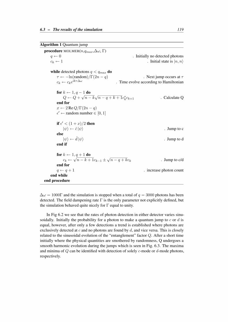
6.3 – The results of the simulation 119
Algorithm 1 Quantum jump
procedure MOLMER(n,qmax,∆ω, Γ)q ← 0 . Initially no detected photonsck ← 1 . Initial state is |n, n〉
while detected photons q < qmax doτ ← −ln(random)/Γ(2n− q) . Next jump occurs at τck ← cke
ikτ∆ω . Time evolve according to Hamiltonian
for k ← 1, q − 1 doQ← Q+
√n− k√n− q + k + 1c∗kck+1 . Calculate Q
end forx← 2 ReQ/Γ(2n− q)ε′ ← random number ∈ [0, 1]
if ε′ < (1 + x)/2 then|ψ〉 ← c |ψ〉 . Jump to c
else|ψ〉 ← d |ψ〉 . Jump to d
end if
for k ← 1, q + 1 dock ←
√n− k + 1ck−1 ±
√n− q + kck . Jump to c/d
end forq ← q + 1 . increase photon count
end whileend procedure
∆ω = 1000Γ and the simulation is stopped when a total of q = 3000 photons has beendetected. The field dampening rate Γ is the only parameter not explicitly defined, butthe simulation behaved quite nicely for Γ equal to unity.
In Fig 6.2 we see that the rates of photon detection in either detector varies sinu-soidally. Initially the probability for a photon to make a quantum jump to c or d isequal, however, after only a few detections a trend is established where photons areexclusively detected at c and no photons are found by d, and vice versa. This is closelyrelated to the sinusoidal evolution of the “entanglement” factor Q. After a short timeinitially where the physical quantities are smothered by randomness, Q undergoes asmooth harmonic evolution during the jumps which is seen in Fig. 6.3. The maximaand minima of Q can be identified with detection of solely c-mode or d-mode photons,respectively.

120 Unexpected coherence
0 0.002 0.004 0.006 0.008 0.01 0.012 0.014 0.0160
10
20
30
40
50Number of photons detected at c
0 0.002 0.004 0.006 0.008 0.01 0.012 0.014 0.0160
10
20
30
40
50Number of photons detected at d
Figure 6.2: The number of photons detected at (upper) detector c and (lower) at detector d.The duration of each “bin” in the stair-diagram is ∆t = 0.0002Γ−1.
0 0.002 0.004 0.006 0.008 0.01 0.012 0.014 0.016−1
−0.8
−0.6
−0.4
−0.2
0
0.2
0.4
0.6
0.8
1
time [sΓ−1]
2<Q
/(Γ
(2n−
q))
Figure 6.3: The time evolution of the “entanglement” variable Q during quantum jumpsrepresented as the normalised quantity 2 ReQ/(Γ(2n− q)) for q = [0, 3000]. Weclearly see the transition from initial randomness to steady harmonic variation.
6.3 – The results of the simulation 121
In fact, the smooth behaviour of Q closely resembles that which one would expectif the cavity modes had been prepared in coherent states instead. If the initial state ofthe system had been the product coherent state
|ψ(0)〉 = |α, β〉 = |α〉 ⊗ |β〉 (6.30)
where |α〉 is the eigenstate of a and |β〉 the eigenstate of b, then the annihilationoperators a and b would have no effect on the kets, i.e., the state would be unchangedduring jumps. However, in-between jumps the state would evolve according to theHamiltonian. The time evolution of a coherent state can be found by writing it in termsof a Fock-state on which the time evolution operator is be applied:
|n(t)〉 = U(t) |n(0)〉 = e−iHt/~ |n(0)〉 (6.31)
For instance, the coherent state |α〉, in terms of the Fock-state is
|α〉 = e−|α|2/2
∞∑n=0
αn√n!|n〉 (3.43)
and the effective Hamiltonian gives the eigenenergy
Ea = 〈Heff,a〉 = ~[ωa − iΓ/2]〈a†a〉 = ~[ωa − iΓ/2]n (6.32)
where we have redefined the energy-origin to get rid of the zero-energy term in H . Thisgives
|α(t)〉 = e−|α|2/2
∞∑n=0
αn√n!|n(t)〉
= e−|α|2/2
∞∑n=0
αn√n!e−iEat/~ |n(0)〉
= e−|α|2/2
∞∑n=0
1√n!
(αe−iωat−Γt/2
)n |n(0)〉
=∣∣∣αe−iωat−Γt/2
⟩(6.33)
The same argument is valid for |β〉, thus the evolution of the two-mode product state is
|α, β〉 →∣∣∣αe−iωat−Γt/2, βe−iωbt−Γt/2
⟩. (6.34)
The rates of the detection events in this case is
γc(d) = Γ[|α|2 + |β|2 ± 2|α||β| cos(∆ωt+ φ)
]e−Γt (6.35)
where the c-numbers α, β are defined as
α = |α|eiφa and β = |β|eiφb (6.36)
and φ = φa − φb is some random relative phase. Then the coherent state-equivalent tothe “entanglement” factor Q is here the term
|α||β| cos(∆ωt+ φ).

122 Unexpected coherence
0 500 1000 15000
0.05
0.1
0.15
0.2
0.25
0.3
0.35
0.4
detected photons q
Figure 6.4: The time evolution of the ck amplitudes, here calculated numerically as |ck|2.The x-axis shows k, where k ∈ [0, q], which increases by unity for every timestep in the simulation, i.e., for every new photon detected. In this plot only theprobabilities at every 100 detection is shown, with increasing k from left to right.As expected, the most likely state of the system is that the 2n− q photons left areequally distributed in the cavities a and b.
It exhibits the same sinusoidal behaviour as Q for the product number state-case, with aperiod equal to the frequency difference of the two cavity modes.2 In the simulationthere are no mean fields (i.e., Q = 0) neither initially nor during the jumps. Butduring the jumps (or detections if you will), mean fields are measured and the resultingentangled state behaves similarly to a product coherent state.
We can also numerically verify that the amplitudes ck evolve smoothly duringjumps, see Fig. 6.4. The figure shows |ck|2 for the kth photon detected, where k ∈ [0, q]increases by unity for every time step in the simulation, i.e., for every new photondetected. In this plot only the probabilities at every 100 detection is shown, withincreasing k from left to right. As expected, the most likely state of the system is thatthe 2n− k photons left are equally distributed in the cavities a and b. That is, |ck|2 isstrongly peaked at k/2.
2 It is quite mind boggling and unintuitive that the amplitude of the coherent state is not reduced by thedetection of photons leaving the cavities, but rather by no photon emission at all! This can be explained byBayesian probability theory where for each time step of no-detection it is more likely that the system (i.e.,source atom) already has emitted the photon and is in the ground state [32].

6.4 – Summary and discussion 123
6.4 Summary and discussion
The conclusion to be drawn from the Mølmer-model is that it is not necessary torequire the cavity modes to be coherent initially. The apparent coherent behaviour is aconsequence of measurement on the state and thereby collapse of the wave function.Feeding the information of which state the system is in, back to the system, will induceentanglement between the cavity modes, thus introducing a coherent behaviour. Anotherthing is that it does not in particular matter what the frequency difference ∆ω is, onlythat it is non-zero. The entanglement will still occur as Q will still be sinusoidal; onlythe period of the oscillations will be affected.
Some of the points Mølmer makes in [31] follows. The physical difference betweenan ensemble of number states and an ensemble of coherent states lies in the ensembleaveraged density matrix. If this is the same for both ensembles, then even if we haveprecise knowledge that there is no mean electric field (i.e., 〈E(+)〉 = 0), we may stillutilize coherent states in the calculations.
Also, formally the one- and two-time expectation values (i.e., 〈a(t)〉 and 〈a†(t)a(t+τ)〉 ∼ g(1)(τ)) obey the same set of equations (through the quantum regression theorem,which we won’t go into). So the application of non-vanishing means produces correctquantitative results, not for one-time means and products like 〈a(t)〉, but for expectationvalues like 〈a†(t)a(t+ τ)〉. In the typical photodetection experiment it is the degree ofsecond-order coherence that is measured. If it uses two single-mode sources that areuncorrelated, like in the Mølmer model, there is no contribution from terms involvinga†b, b†a. However, the relative intensity correlation function will contain a termproportional to 〈a†(t)a(t+ τ)b†(t+ τ)b(t)〉 which is non-vanishing and proportionalto the product of 〈a†(t)a(t + τ)〉 and 〈b†(t)b(t + τ)〉 (similar to what we saw forthe intensity interferometer in section 2.3). This contribution can be mistaken for aninterference peak due to a non-vanishing mean field, i.e., that the light beam impingingon the detectors is in a coherent state, when in fact this is not the case.
Mølmer also puts forward that a closer scrutiny of the mechanism behind manyquantum optical experiments will reveal that it is not necessary to use light beamsinitially prepared in coherent states, as it is the backaction of the information gained inmeasuring the system that is the true source of entanglement. In addition it is likely thatno coherent electric fields in the optical regime has been observed yet, or even created,as that would require classical oscillators (i.e., a moving charge distribution) and notquantum systems with a vanishing dipole moment. However, for low non-opticalfrequencies, classically moving charged objects do exist and they do emit coherentradiation.
Another interesting point is that in the simulations of the Mølmer model, theentanglement is not so fragile as to be destroyed by the influence of the environment, inthis case by physical observation. Coherent states are usually considered to be morerobust in this sense as the act of observation of the field leaves the state unaltered (whichwe have discussed in both the previous section and in section 3.4).

Chapter 7
Concluding remarks
For brevity the reader is referred to the end-section of each chapter for a detailedsummary of our investigation. Here we will simply try to answer the questions posed inthe Introduction.
What is coherence and how is it quantified, calculated, measured? In this workboth the classical and the quantum mechanical side of coherence has been lookedinto. A collective term may be optical coherence theory, including the degrees ofNth-order coherence, of which only the first two has been studied here. So we knowthe mathematics of coherence; in the classical sense it is the time average of twofunctions multiplied together and whenever these behave “similarly” there is a positive,or constructive, addition to the average, and a negative, destructive, addition when theybehave “dissimilarly”. In the quantum mechanical sense coherence is calculated asthe expectation value of the field operators. Nevertheless, the term coherence in itselfis a concept that is somewhat hard to quantify the precise meaning of. To speak inthe broadest sense, optical coherence theory is a statistical description of fluctuationsthat can be found in any optical field in nature [33]. Coherence can be said to be themanifestation of correlations between such fluctuations.
In section 2.2 we saw that the degree of first-order coherence can be measured byfinding the visibility of the interference fringes that arise from superposing two electricfields. g(1)(τ) can also be found by measuring the power spectral density of the field.The intensity interferometer measures the degree of second-order coherence, as seen insection 2.3.
What is the difference between coherent light and incoherent light? Coherentlight in this work is regarded as having degrees of first- and second-order coherenceequal to unity
|g(1)(τ)| = 1 and g(2)(τ) = 1. (1.70)
It was found in sections 1.4 and 4.1 that only the classical ideal wave and single-modelight in a coherent state is coherent (but this can also be shown for multi-mode light).Far above threshold, laser light is approximately coherent as well (section 5.3).
125
126 Concluding remarks
Can light be something in-between? By referring to the degree of first-order coher-ence, light can be coherent, incoherent or partially coherent, as seen from the derivationof the limits in sections 1.3 and 3.2. But from the definitions and the criterion Eq. (1.70)it is seen that light is either second-order coherent or second-order incoherent.
Can coherence be explained by both classical theory and quantum mechanics?Are the explanations equivalent? The full theory of coherence covers both theclassical electromagnetic theory and the quantum optical theory. In our calculationsof g(1)(τ) and g(2)(τ) for light in the coherent state and in the mixed thermal state(section 4), the results were analogous to their classical counterparts, the stable, idealwave and chaotic light. However, one must keep in mind that the quantum theory carrieswith it inevitable vacuum fluctuations that are not present in classical theory. For thethermal state an additional factor representing a source-correlation correction turned up.
Does it matter which statistical properties the light has? We saw in section 4.2 thatfor light in a Fock state, which does not have a classical equivalent, its photon statisticsled to classically illegal values of g(2)(τ). This gives rise to photon antibunching, apurely quantum mechanical characteristic.
The unasked questions
Along the way we also stumbled upon other key points of interest, like the HanburyBrown-Twiss effect, which was shown in section 2.3 to be an excess in the intensitycorrelation due to classical chaotic light having g(2)(0) = 2. In the quantum picturethis was seen to manifest as photon bunching. Coherent light did not exhibit neither.
How similar is laser radiation really to classical coherent light? The route to theanswer goes first through the coherent state. Far above threshold the laser beam has thesame photon statistics and degrees of first- and second-order coherence as the coherentstate, albeit with random perturbations due to spontaneous emission. The laser is agood approximation to classical coherent light if one accepts the minimal uncertaintyin amplitude and phase as negligible, and the phase drift due to spontaneous emissionas slow enough to be disregarded.
Do we really need the coherent states to describe the coherence properties in light?In section 6 we investigated the Mølmer-model in which coherence is shown to beinduced by the process of updating the system state with information regarding itsphoton emission. I.e., entanglement is created, where initially the two subsystemswere uncorrelated. The induced coherence was shown to be identical to the coherencewhich the system would exhibit if it was initially in a coherent state. So, at least in thisexample the coherent state was not necessary, but it did provide a shorter and moreconvenient path to measuring the coherence.
The unanswered questions
Is there merit to Mølmer’s claim that coherent light has never been observed?
127
Are there other models where one can test the hypothesis that coherent states arenot necessary for finding coherence?
Is there a better way to derive the properties of the laser without resorting to thecomplex and convoluted machinery of the density operator method?
Is it justifiable to assume no interactions between the atoms in the laser gain mediumat shorter times ∼ τ?
Will not the rate of spontaneous emission by the laser gain medium be affectedby the presence of the strong laser field so that an exponential decay (Eq. (5.19)) isinadequate?
The author leaves these questions, and others, in the hands of future students of quantumoptics.

Appendix A
Determining the statisticalproperties of chaotic light
The following are the derivation of the Lorentzian and the Gaussian frequency distribu-tions used for the degree of first-order coherence in section 1.3.1.
A.1 Collision (pressure) broadening
Again consider a gas of atoms interacting with a radiation field. If there are othermechanisms in addition to spontaneous and stimulated transitions that depletes theexcited state, the spectral lines will be broadened, i.e. the allowed frequency rangeincreases, ω′k = ωk + ∆ω. One such broadening mechanism is collisions between theatoms. Inelastic collisions can have quite a complicated effect on the energy levelsand wavefunctions on the atom, so we will only consider elastic collisions that leavesthe atom in the same energy level as before and only changes the phase of the atomicwavefunction.
So, picture a particular excited atom radiating light at frequency ω0. In betweeneach collision the frequency will stay the same, but the phase of the radiated wave isnow unrelated to the phase before the collision. The occurrence of collisions betweenthe atoms in a gas is a random process and the probability that an atom has a period τof free flight between collisions is given by the kinetic theory of gases
p(τ)dτ =1τ0e−τ/τ0dτ. (A.1)
The mean time τ0 of free flight is a function of the number density of the atoms andof the relative velocity of between pairs of atoms, both of which also depend on thetemperature and pressure of the gas, and as such are a major source of informationabout physical conditions in stellar atmospheres.
The point of using a model of collision broadened light is that the line intensityis proportional to a Lorentzian frequency distribution. To be specific, assume that the
129

130 Determining the statistical properties of chaotic light
wave train radiated by an atom has a complex amplitude of the form
E(t) = E0e−i(ω0t+φ(t)) (A.2)
where the phase φ(t) is constant in the periods of free flight, but changes abruptly eachtime a collision occurs. The total electric field amplitude produced by a large number νof atoms, all radiating with the same amplitude E0 and frequency ω0, is then
E(t) = E1(t) + E2(t) + . . .+ Eν(t)
= E0e−iω0t
[eiφ1(t) + eiφ2(t) + . . .+ eiφν(t)
](1.58)
where all the ν atoms are equivalent. The real electric field described by Eq. (1.58)consists of a carrier wave of frequency ω0 which is modulated by the sum of the randomphases of each atom.
Because of the ergodic nature of light we can then view the first-order correlationfunction of the light, which is a time average of the field emitted by an atom, as astatistical average over each ν atom,
〈E∗(t)E(t+ τ)〉 = E20e−iω0τ
⟨[e−iφ1(t) + e−iφ2(t) + . . .+ e−iφν(t)
]×[eiφ1(t+τ) + eiφ2(t+τ) + . . .+ eiφν(t+τ)
]⟩.
(A.3)
The angle-bracket notation will now be used for both the time average and the statisticalaverage. In multiplying out the contents of the brackets the cross terms of differentatoms will average to zero, since they are independent and are not correlated. Providedthat τ is less than the mean period of free flight between each collision, only cross termscontaining the phases φi(t) and φi(t+ τ) from the same atom i will contribute to theaverage
〈E∗(t)E(t+ τ)〉 = E20e−iω0τ
ν∑i=1
〈ei(φi(t+τ)−φi(t))〉 = ν〈E∗i (t)Ei(t+ τ)〉. (A.4)
In other words the correlation function of the entire beam of light is determined by thesingle-atom contribution. To proceed we need to find an expression for the single-atomcorrelation function. This term is zero if a collision occurs within the delay time τ ,since the wave train then has a phase unrelated to that before. The only contribution iswhen the atom has a period of free flight longer than τ , and the probability for this isgiven by Eq. (A.1). So the correlation function can be written as
〈E∗(t)E(t+ τ)〉 = νE20e−iω0τ
∫ ∞τ
dτ ′p(τ ′) = νE20e−iω0τ−τ/τc (A.5)
where we have renamed the mean period of free flight τ0 of the atom to the coherencetime τc since these are for all intents and purposes equivalent.
The degree of first-order correlation is the normalised correlation function
g(1)(τ) = e−iω0τ−|τ |/τc . (1.40)
In the last step here the correlation function has been generalised for both positive andnegative τ according to the symmetry relation Eq. (1.31).

A.2 – Doppler broadening 131
A.2 Doppler broadening
If Doppler broadening is the main mechanism of spread in the frequency spectrumof chaotic light, the calculation is slightly different from the above. Consider againa gas of atoms interacting with photons. A stationary atom will absorb a photon thatcarries the appropriate momentum ~k0, where k0 = ω0/c. If the atom is moving at anon-relativistic velocity and v is the component of the velocity along the line of sight,the frequency of the emitted light is, to first order in v/c,
ω = ω0
(1 +
v
c
)(A.6)
where v is negative if the atom is receding from the observer. This is known as thefirst-order Doppler effect. Another way to view this effect is that light is absorbed onlywhen its frequency ω differs from ω0 by the Doppler shift appropriate to the initialatomic velocity. So a spread in the atomic velocity of the gas will result in a spread ofthe absorbed frequencies.
To sum it up, the effect of collision broadening is to alter the phase angle φ to somerandom value completely unrelated to the previous, while the frequency ω0 stays thesame. In contrast, Doppler broadening results in a shift from ω0 by amounts determinedby the atomic velocities, while the phase angles have fixed, but randomly distributed,values.
If the gas has the absolute temperature T , the number of atoms, dN , with velocitiesbetween v and v + dv is given by Maxwell’s velocity distribution
dN = N0e−Mv2/(2kBT )dv (A.7)
where kB is Boltzmann’s constant, M is the atomic mass and N0 is a constant. It isconvenient to normalise this to the total number of atoms ν, for reasons that will soonbe apparent,
ν =∫ ν
0dN = N0
∫ ∞−∞
e−Mv2/(2kBT )dv = N0
√2πkBTM
(A.8)
which gives
N0 = 2ν√
M
2πkBT(A.9)
Inserting dv = (c/ω0) dω (from Eq. (A.6)) into Eq. (A.7) we find
dN = N0c
ω0e−Mc2(ω−ω0)2/(2kBTω
20)dω. (A.10)
If we define
∆ = ω0
√kBT
Mc2(A.11)

132 Determining the statistical properties of chaotic light
Maxwell’s velocity distribution as a function of the angular frequency takes on the form
dN = ν(2π∆2)−1/2e−(ω−ω0)2/(2∆2)dω (A.12)
In keeping with Eq. (1.58), the total electric field of a linearly polarised light beamcan be written as
E(t) = E0
ν∑i=1
e−i(ωit+φi) (A.13)
where E0 and φi are the fixed amplitude and phase angle of the wave radiated by theith atom, and the angular frequency ωi is Doppler shifted from ω0. The first-ordercorrelation function is thus
〈E∗(t)E(t+ τ)〉 = E20
ν∑i,j=1
〈ei(ωit−φi−ωj(t+τ)+φj)〉 = E20
ν∑i=1
e−iωiτ , (A.14)
where the terms for i 6= j average to zero since the phase angles are randomly distributed.The sum can be approximated to an integral by assuming that exp (−iωiτ) will vary solittle as to be almost constant in an interval of frequencies ∆ω emitted by ∆N sources,∑
i
fi ≈∑i
fi ·∆N
And if this interval approaches infinitesimal, we get∑i
fi ·∆N∆ω
∆ω →∫f(ω)
dNdω
dω.
Then we insert Eq. (A.12), which gives
〈E∗(t)E(t+ τ)〉 = νE20(2π∆2)−1/2
∫ ∞0
e−iωτe−(ω0−ω)2/(2∆2)dω
= νE20e−iω0τ− 1
2∆2τ2
, (A.15)
where the last step is achieved by completing the square in the exponential function andsolving the Gaussian integral with the substitution
ω → ω′ = (2∆2)−1/2(ω − ω0), dω′ = (2∆2)−1/2dω.
This change of variables will give the lower integration limit
ω = 0⇒ ω′ = −(2∆2)−1/2ω0,
which according to basic dimension analysis is around −106. This allows us to approxi-mate the integral over the entire real line,∫ ∞
0dω →
∫ ∞−∞
dω′.

A.2 – Doppler broadening 133
Noting that ∆ has units [rad/s] a convenient definition of the coherence time [1] is
τc =√π
∆. (A.16)
In a similar form of Eq. (1.40), we have found the degree of first-order coherence forDoppler broadened light
g(1)(τ) = e−iω0τ−π2 (τ/τc)2 . (1.41)

Appendix B
Selected tedious calculations
B.1 The energy of the classic radiation field
The total energy of the radiation field in the cavity with volume V = L3 from sec-tion 1.1.2, is
HR =12ε0
∫V
(E2 + c2B2)dr. (1.20)
Before starting this potentially unpleasant integration, we take a moment to considerthe type of integral we will end up with. If the scalar products are between differentmodes k,k′, there will be terms of the form
1V
∫Ve±i(k+k′)rdr = δk(−k′) (B.1)
for cross terms of akλak′λ′ or c.c.1, and
1V
∫Ve±i(k−k′)rdr = δkk′ (B.2)
for cross terms of akλa∗k′λ′ or c.c., These are identities of the Dirac delta function andgive no contribution unless k′ is either −k or k, respectively. The frequency ωk isthe same in either case. We will also get the scalar product of the unit polarisationvectors which will further simplify the matters since the two different directions λ, λ′
are perpendicular, and in addition
(k× εkλ) · (k× ε±kλ′) = (k · k)(εkλ · ε±kλ′) = ±k2δλλ′ . (B.3)
The calculation goes as follows, where we denote the primed indices by priming thevariable itself and χ = k · r− ωkt etc,
|E|2 ∼∑kk′
∑λλ′
ε · ε′[aa′ei(χ+χ′) + aa′∗ei(χ−χ
′)
+ a∗a′e−i(χ−χ′) + a∗a′∗e−i(χ+χ′)
], (B.4)
1The abbreviation c.c. stands for complex conjugated.
134

B.2 – The Lie formula 135
and integrating gives
1V
∫V|E|2dr
∼∑kk′
∑λλ′
δλλ′[aa′δk,−k′e
−2iωkt + aa′∗δk,k′ + a∗a′δk,k′ + a∗a′∗δk,−k′e−iωkt
]=∑k
∑λ
[akλa−kλe−2iωkt + akλa
∗kλ + a∗kλakλ + a∗kλa
∗−kλe
2iωkt] (B.5)
The same procedure gives for the magnetic field
|B|2 ∼∑kk′
∑λλ′
(k× ε) · (k′ × ε′)ωkωk′
[aa′ei(χ+χ′) + aa′∗ei(χ−χ
′)
+ a∗a′e−i(χ−χ′) + a∗a′∗e−i(χ+χ′)
], (B.6)
and after integrating
1V
∫Vc2|B|2dr
∼∑kk′
∑λλ′
c2
ωkωk′δλλ′
[aa′k(−k′)δk,−k′e
−2iωkt + aa′∗kk′δk,k′
+ a∗a′kk′δk,k′ + a∗a′∗k(−k′)δk,−k′e2iωkt
]=∑k
∑λ
[−akλa−kλe−2iωkt + akλa
∗kλ + a∗kλakλ − a∗kλa∗−kλe
2iωkt] (B.7)
The resulting total radiative energy is then simply
HR =∑k
∑λ
12
~ωk(akλa∗kλ + a∗kλakλ) =∑k
∑λ
~ωkakλa∗kλ (B.8)
B.2 The Lie formula
Every now and then in quantum mechanics we will need to evaluate expressions on theform
eX Y e−X (B.9)
It is fairly easy to show that the solution is
eX Y e−X = Y + [X, Y ] +12!
[X, [X, Y ]] +13!
[X, [X, [X, Y ]]] + . . . (B.10)
Proof is found by considering the operator
F (λ) = eλX Y e−λX . (B.11)

136 Selected tedious calculations
The trick is to do a Taylor expansion, so we need the derivative
dFdλ
= eλXXY e−λX − eλX Y Xe−λX = XF − F X = [X, F ], (B.12)
and the second derivative is found to be
d2F
dλ2=
ddλ
[X, F ] = [X, [X, F ]]. (B.13)
This pattern is repeated and we find that the Taylor expansion is
F (λ) = F (0) + λF ′(0) +λ2
2!F ′′(0) +
λ3
3!F ′′′(0) . . . (B.14)
Finally this gives the Lie formula
eλX Y e−λX = Y + [X, Y ] +λ
2![X, [X, Y ]] +
λ
3![X, [X, [X, Y ]]] + . . . (B.15)
B.3 Solving the eigenvalue problem
We now solve the eigenvalue problem of section 5.1.1 to find the system state amplitudesCan(t) and Cbn+1(t) from Eq. (5.5).
The effective Hamiltonian is defined as
H =12
~ω0σz + ~Ωa†a+ ~g(a†σ + aσ†) (B.16)
or
H = ~(
12ω0 + Ωn g
√n+ 1
g√n+ 1 −1
2ω0 + Ω(n+ 1)
)= ~
(12(ω0 − Ω) + Ω(n+ 1/2) g
√n+ 1
g√n+ 1 1
2(ω0 − Ω) + Ω(n+ 1/2)
)= ~
(Ω(n+ 1/2) g
√n+ 1
g√n+ 1 Ω(n+ 1/2)
)(B.17)
where the last step is due to assumed resonance.
The next move is to find the eigenvalues ~λ of the Hamiltonian,
det(H − ~λ) = det ~(
Ω(n+ 1/2)− λ g√n+ 1
g√n+ 1 Ω(n+ 1/2)− λ
)= ~(Ω(n+ 1/2)− λ)2 − ~(g
√n+ 1)2
≡ 0 (B.18)
This gives the two eigenvalues
λ1 = Ω(n+ 1/2) + g√n+ 1,
λ2 = Ω(n+ 1/2)− g√n+ 1
(B.19)

B.3 – Solving the eigenvalue problem 137
For each eigenvalue there is an eigenvector that can be found from
(H − ~λi)vi = 0 (i = 1, 2) (B.20)
The straight forward calculation yields
v1 =[
11
]for λ1 = Ω(n+ 1/2) + g
√n+ 1
v2 =[
1−1
]for λ2 = Ω(n+ 1/2)− g
√n+ 1
(B.21)
Then the time-dependent state can be written in terms of the eigenvalues andeigenvectors as
|ψ(t)〉 = c1v1e−iλ1t + c2v2e
−iλ2t (B.22)
and with the initial condition that the atoms are in the upper laser level at t = 0, wehave
|ψ(0)〉 = c1v1 + c2v2 =[10
]= |a〉 . (B.23)
This gives
c1
[11
]+ c2
[1−1
]=[10
]⇒ c1 = 1/2 and c2 = 1/2 (B.24)
and
|ψ(t)〉 =12
[11
]e−i[Ω(n+1/2)+g
√n+1]t +
12
[1−1
]e−i[Ω(n+1/2)−g
√n+1]t (B.25)
Finally, the amplitudes for the atom being in state |a, n〉 or |b, n+ 1〉 after time t are,respectively,
Can(t) = cos(g√n+ 1t)e−iΩ(n+1/2)t
Cbn+1(t) = −i sin(g√n+ 1t)e−iΩ(n+1/2)t
(B.26)
As a matter of computational simplicity we can change from the Schrödinger picture tothe Interaction picture i.e., pulling the exponentials in Eq. (B.26) into the state vector,thus
Can(t) = cos(g√n+ 1t)
Cbn+1(t) = −i sin(g√n+ 1t).
(B.27)

Appendix C
Source code listings
C.1 Script for calculating coherences
The following listing was used to calculate the intensity correlations for the Michelsonstellar interferometer and the intensity interferometer. Eqs.(2.46) and (2.48) was usedfor a Lorentzian frequency distribution, and for a Gaussian frequency distribution theEqs.(2.47) and (2.49). The results are plotted in Figs. 2.7 and 2.9.
Coherence.m1 f u n c t i o n D = c o h e r e n c e
c l o s e a l l ; c l c ; c l e a r ;
r = input (’Enter \n 1 for intensity int. \n 2 for michelson int.’ ) ;
i f r == 1 , funk = ’intensity’ ;e l s e i f r == 2 , funk = ’michelson’ ;end
f r e q = [’g’ ,’l’ ] ;11 f req_name = ’Gaussian’ , ’Lorentzian’ ;
% c o l o r s f o r t h e p l o tc l r = ’-b’ , ’-r’ , ’--g’ , ’-m’ ;
ang le = [ 0 . 0 0 4 7 0 .047 0 . 4 7 ] ;
j = 0 ;r = 1 ;
21 f o r n = 1 : l e n g t h ( f r e q )f o r s = 1 : 1 : l e n g t h ( ang le ) % want t o compare d i r e c t l y 3 d i f f e r e n t
j = j + 1 ; % a n g l e s o f t h e same o r d e r o f magn i tude
param = i n i t i a l i s e P a r a m ( 10^(1− r ) , ang le ( s ) ) ;C j , 1 = c a l c u l a t i o n ( funk , param , f r e q ( n ) ) ;f i g l a p p j , 1 = s t r c a t ( f req_name ( n ) , . . .
’: $\theta=’ , num2str ( ang le ( s ) ) ,’"$’ ) ;
end31 end
r = 1 ;
138

C.1 – Script for calculating coherences 139
f o r t = 1 : 3 : j %p l o t 3 a n g l e s i n t h e same imagef i g u r e ;hold on ;
p l o t ( param . d , C t , 1 : , c l r 1 ) ;i f j > 1 , p l o t ( param . d , C t + 1 , 1 : , c l r 2 ) ;
l a p p = [ f i g l a p p t , 1 , f i g l a p p t + 1 , 1 ] ; end41 i f j > 2 , p l o t ( param . d , C t + 2 , 1 : , c l r 3 ) ;
l a p p = [ f i g l a p p t , 1 , f i g l a p p t +1 ,1 , f i g l a p p t + 2 , 1 ] ; end
legend ( l app , ’Interpreter’ ,’latex’ ,’FontSize’ , 1 4 ) ;x l a b e l (’$d$ [m]’ , ’Interpreter’ ,’latex’ ,’FontSize’ , 1 4 ) ;y l a b e l (’$C$’ , ’Interpreter’ ,’latex’ ,’FontSize’ , 1 4 ) ;s e t ( gca , ’FontSize’ , 1 4 ) ;
i f t <= f l o o r ( j / 2 )f r e k v = f r e q ( 1 ) ;
51 e l s ei f l e n g t h ( f r e q ) > 1 , f r e k v = f r e q ( 2 ) ; end
end
t h = num2str ( ang le ( r ) ) ;o u t f i l e = [ funk ’_’ f r e k v ’_’ num2str ( param . I _ a ) . . .
’Ia’ num2str ( param . I_b ) ’Ib_’ t h ( 3 : end ) ] ;%s a v e i m a g e s ( gc f , o u t f i l e ) ;r = r + 3 ;i f r > l e n g t h ( ang le ) , r = 1 ; end
61 endend
% I n i t i a l i s e t h e r e q u i r e d p a r a m e t e r s f o r t h e c a l c u l a t i o n sf u n c t i o n param = i n i t i a l i s e P a r a m ( ang le )
param . c = 3 e8 ;lambda = 540 e−9; % a g u e s s !param . k = 2∗ pi / lambda ; % k = w / c = 2 p i / L
a r c s e c o n d = pi / 6 4 8 0 0 0 ; % r a d i a n s71 param . a r c s e c = a r c s e c o n d ;
param . t h e t a = ang le∗ a r c s e c o n d ;
d = −0 : 0 . 0 1 : 3 ; % d t h e t a = r_a − r_bparam . d = d∗1 e0 ; % t h e b a s e l i n e 10^1param . d_c = 1e−6; % c o h e r e n c e l e n g t h o f t h e r m a l l i g h tparam . r _ a = param . d∗1e−7; % r_a = c∗ t au_a = d . L / L = d∗ cos ( p i / 2 )% param . r_b = d ; % r_b = r_a − d t h e t aparam . I _ a = 1 ;param . I_b = 1 ;
81
end
% R e t u r n s t h e d eg re e o f f i r s t −o r d e r c o h e r e n c ef u n c t i o n r e s u l t = g1 ( sou rce , d i s t r , j , s )
d_c = s . d_c ;r _ a = s . r _ a ;d = s . d ;c = s . c ;t h e t a = s . t h e t a ;
91 k = s . k ;
s w i t c h d i s t rc a s e ’g’ %g a u s s i a n
i f strcmp ( sou rce ,’a’ ) %ar e s u l t = exp(− i ∗k∗ r _ a ( j ) − pi / 2∗ ( r _ a ( j ) / d_c ) ^ 2 ) ;
e l s e i f strcmp ( sou rce ,’b’ )r e s u l t = exp(− i ∗k ∗ ( r _ a ( j ) − d ( j )∗ t h e t a ) . . .
− pi / 2∗ ( r _ a ( j ) / d_c − d ( j )∗ t h e t a / d_c / c ) ^ 2 ) ;

140 Source code listings
end101 c a s e ’l’ %l o r e n t z i a n
i f strcmp ( sou rce ,’a’ )r e s u l t = exp(− i ∗k∗ r _ a ( j ) − abs ( r _ a ( j ) / d_c ) ) ;
e l s e i f strcmp ( sou rce ,’b’ )r e s u l t = exp(− i ∗k ∗ ( r _ a ( j ) − d ( j )∗ t h e t a ) . . .
− abs ( r _ a ( j ) / d_c − d ( j )∗ t h e t a / d_c / c ) ) ;end
endend
111 % R e t u r n s d eg re e o f second−o r d e r c o h e r e n c ef u n c t i o n r e s u l t = g2 ( sou rce , d i s t r , j , s )
d_c = s . d_c ;r _ a = s . r _ a ;d = s . d ;c = s . c ;t h e t a = s . t h e t a ;
s w i t c h d i s t rc a s e ’g’ %g a u s s i a n
121 i f strcmp ( sou rce ,’a’ )r e s u l t = 1 + exp(−pi ∗ ( r _ a ( j ) / d_c ) ^ 2 ) ;
e l s e i f strcmp ( sou rce ,’b’ )r e s u l t = 1 + exp(−pi ∗ ( r _ a ( j ) / d_c − d ( j )∗ t h e t a / d_c / c ) ^ 2 ) ;
endc a s e ’l’ %l o r e n t z i a n
i f strcmp ( sou rce ,’a’ )r e s u l t = 1 + exp (−2∗abs ( r _ a ( j ) / d_c ) ) ;
e l s e i f strcmp ( sou rce ,’b’ )r e s u l t = 1 + exp (−2∗abs ( r _ a ( j ) / d_c − d ( j )∗ t h e t a / d_c / c ) ) ;
131 endend
end
% C a l c u l a t e t h e c o r r e l a t i o n f u n c t i o n f o r i n t e n s i t y i n t & Miche l son i n tf u n c t i o n C = c a l c u l a t i o n ( funk , s , f r e q )
d = s . d ;I _ a = s . I _ a ;I_b = s . I_b ;
141 k = s . k ;t h e t a = s . t h e t a ;
s w i t c h funkc a s e ’intensity’
f o r j = 1 : l e n g t h ( d )C( j ) = I _ a ^2∗g2 (’a’ , f r e q , j , s ) . . .
+ I_b ^2∗g2 (’b’ , f r e q , j , s ) . . .+ I _ a ∗ I_b ∗ ( 2 . . .
+ g1 (’a’ , f r e q , j , s )∗ conj ( g1 (’b’ , f r e q , j , s ) ) . . .151 + conj ( g1 (’a’ , f r e q , j , s ) )∗ g1 (’b’ , f r e q , j , s ) ) ;
C( j ) = C( j ) / ( I _ a + I_b ) ^ 2 ;end
c a s e ’michelson’f o r j = 1 : l e n g t h ( d )
C( j ) = I _ a ∗ (1 + r e a l ( g1 (’a’ , f r e q , j , s ) ) ) . . .+ I_b ∗ (1 + r e a l ( g1 (’b’ , f r e q , j , s ) ) ) ;
C( j ) = C( j ) / ( I _ a + I_b ) ;end
end161 end

C.2 – Script for calculating Monte Carlo quantum jumps 141
C.2 Script for calculating Monte Carlo quantum jumps
The following Matlab-script was used to compute the Monte Carlo quantum jumpdescribed by Algorithm 1 in section 6.2. The results of the simulation is plotted inFigs.6.2, 6.3 and 6.4.
molmer.mc l e a r ; c l c ; c l o s e a l l ;
% I n i t i a l v a l u e s , a t t = 0c_0 = 1 ;c_1 = 0 ;Q_0 = 0 ;Gamma = 1 ;d e l t a = 1000∗Gamma ;
9
n = 1 e5 ; % Number o f p h o t o n s i n each c a v i t yq_max = 3000 ; % When t h e measurement s t o p sq = 0 ;t = 0 ;
% I n i t i a l i s e v e c t o r s f o r enhanced per fo rmancec_k = z e r o s ( q_max , 1 ) ; % complex a m p l i t u d eQ = z e r o s ( q_max , 1 ) ; % <\ dagger a b>t a u = z e r o s ( q_max , 1 ) ;
19 c _ a t _ t = z e r o s ( q_max , 1 ) ; % jumps t o c a t t i m e td _ a t _ t = z e r o s ( q_max , 1 ) ; % jumps t o d a t t i m e tc k _ a l l = z e r o s ( q_max , q_max ) ; % a m p l i t u d e evo . f o r a l l t
c_k ( 1 , 1 ) = c_0 ;Q( 1 , 1 ) = Q_0 ;t a u ( 1 , 1 ) = 0 ;
jump2c = 0 ;jump2d = 0 ;
29
% Temporary s t o r a g etempQ_c = Q;temp_c = c_k ;tempQ = 0 ;
i d x = 1 ;
whi le q < q_max
39 c k _ a l l ( : , i d x ) = c_k ;
e p s i l o n = rand ( 1 ) ;t a u ( i d x ) = −l o g ( e p s i l o n ) / ( Gamma∗ (2∗n−q ) ) ;
% Time i s now : t = t a u ( q )t = t + t a u ( i d x ) ;
% Time e v o l u t i o n o f t h e a m p l i t u d e s by e f f e c t i v e H a m i l t o n i a nc_k = exp ( i ∗ ( 0 : q_max−1)∗ d e l t a ∗ t a u ( i d x ) ) ’ . ∗ c_k ;
49 c_k = c_k . / norm ( c_k ) ;
% The f i r s t jump goes t o c , s i n c e t h e r e i s a 50% chance e i t h e r way :% Remember t h a t when Q == 0 t h e s t a t e i s n o t e n t a n g l e d , and i t% s h o u l d be e q u a l l y l i k e l y t o jump e i t h e r t o c or d !i f q == 0
Q( i d x ) = 0 ;jumpSign = +1;jump2c = jump2c + 1 ;

142 Source code listings
c _ a t _ t ( i d x ) = 1 ;59
e l s e% C a l c u l a t e Q t o f i n d t h e d i r e c t i o n o f t h e n e x t jumpf o r k = 0 : q−1
tempQ_c ( k +1) = s q r t ( n−k )∗ s q r t ( n−q+k + 1 ) . . .∗ conj ( c_k ( k +1) )∗ c_k ( k + 2 ) ;
endtempQ = sum ( tempQ_c ) ;Q( i d x ) = 2∗ r e a l ( tempQ ) / ( Gamma∗ (2∗n−q ) ) ;
69 e = rand ( 1 ) ;
i f e < (1 + Q( i d x ) ) / 2 % Jump t o cjumpSign = +1;jump2c = jump2c + 1 ;c _ a t _ t ( i d x ) = 1 ;
e l s e % Jump t o djumpSign = −1;jump2d = jump2d + 1 ;
79 d _ a t _ t ( i d x ) = 1 ;
endend
% C a l c u l a t e t h e a m p l i t u d e s o f t h e new s t a t e a f t e r jumpf o r k = 0 : q+1
i f k == 0temp_c ( k +1) = jumpSign∗ s q r t ( n−q+k )∗ c_k ( k + 1 ) ;
e l s e i f k == q+189 temp_c ( k +1) = s q r t ( n−k +1)∗ c_k ( k ) ;
e l s etemp_c ( k +1) = s q r t ( n−k +1)∗ c_k ( k ) . . .
+ jumpSign∗ s q r t ( n−q+k )∗ c_k ( k + 1 ) ;end
end
% Update t h e s t a t e a m p l i t u d e sc_k = temp_c . / norm ( temp_c ) ;
99 i d x = i d x + 1 ;q = q + 1 ;
end
% P l o t t i m e e v o l u t i o n o f 2ReQ / ( Gamma(2 n−q ) )f i g u r e ( 1 ) ;t ime = l i n s p a c e ( 0 , t , l e n g t h (Q)−1) ;p l o t ( t ime ,Q( 1 : end−1) ) ;x l a b e l (’time $[s\Gamma^-1]$’ , ’Interpreter’ , ’latex’ ) ;
109 y l a b e l (’$2\Re Q/(\Gamma(2n-q))$’ , ’Interpreter’ , ’latex’ ) ;
o u t f i l e = ’molmer_timeEvolQ’ ;s a v e i m a g e s ( 1 , o u t f i l e ) ;
% P l o t t i m e e v o l u t i o n o f | c_k | ^ 2f i g u r e ( 2 ) ; hold a l l ; f o r j = 1 : 1 0 0 : q_max , p l o t ( abs ( c k _ a l l ( : , j ) ) ) ; endxl im ( [ 0 q_max / 2 ] ) ; y l im ( [ 0 0 . 4 ] ) ;x l a b e l (’detected photons $q$’ , ’Interpreter’ , ’latex’ ) ;y l a b e l (’probability $\lvert c_k \rvert^2$’ , ’Interpreter’ , ’latex’ ) ;
119
o u t f i l e = ’molmer_timeEvolck2’ ;s a v e i m a g e s ( 2 , o u t f i l e ) ;
d t = 0 .0002∗Gamma^−1;

C.2 – Script for calculating Monte Carlo quantum jumps 143
n b i n s = f l o o r ( sum ( t a u ) / d t ) ;i n t e r v a l l = f l o o r ( l e n g t h ( c _ a t _ t ) / n b i n s ) ;
c_pho ton = z e r o s ( nb ins , 1 ) ;d_photon = z e r o s ( nb ins , 1 ) ;
129
f o r j = 1 : n b i n sc_pho ton ( j ) = sum ( c _ a t _ t ( ( j −1)∗ i n t e r v a l l +1 : j ∗ i n t e r v a l l ) ) ;d_photon ( j ) = sum ( d _ a t _ t ( ( j −1)∗ i n t e r v a l l +1 : j ∗ i n t e r v a l l ) ) ;
end
f i g u r e ( 3 ) ;t ime = l i n s p a c e ( 0 , t , n b i n s ) ;s u b p l o t ( 2 , 1 , 1 ) , s t a i r s ( t ime , c_photon , ’b’ ) ;t i t l e (’Number of photons detected at $c$’ , ’Interpreter’ , ’latex’ ) ;
139 yl im ( [ 0 5 0 ] ) ;s u b p l o t ( 2 , 1 , 2 ) , s t a i r s ( t ime , d_photon , ’r’ ) ;t i t l e (’Number of photons detected at $d$’ , ’Interpreter’ , ’latex’ ) ;y l im ( [ 0 5 0 ] ) ;
o u t f i l e = ’molmer_photonDetec’ ;s a v e i m a g e s ( 3 , o u t f i l e ) ;

References
[1] Loudon R.. The quantum theory of light. Oxford Univ. Press3rd ed. 2003.
[2] Goodman J.W.. Statistical optics. Wiley New York 1985.
[3] Fox M.. Quantum Optics: An Introduction. Oxford Univ. Press, USA 2006.
[4] Mitchell ACG, Zemansky MW. Resonance Radiation and Excited Atoms. Cam-bridge Univ. Press, London 1934.
[5] Hanbury Brown R., Davis J., Allen LR, Rome JM. The stellar interferometer atNarrabri Observatory-II. The angular diameters of 15 stars Mon. Not. R. Astron.Soc.. 1967;137.
[6] Richichi A., Percheron I.. CHARM: A Catalog of High Angular ResolutionMeasurements A&A. 2002;386:492–503.
[7] Hanbury Brown R.. The intensity interferometer. Its applications to astronomy.Taylor & Francis, London 1974.
[8] Paganin D.M.. Coherent x-ray optics. Oxford University Press, USA 2006.
[9] Scully M.O., Zubairy M.S.. Quantum Optics. Cambridge Univ. Press 1997.
[10] Michelson AA. An Interferometer for Measuring Stellar Diameter Astrophys. J..1920;51:257.
[11] Michelson AA. On the application of interference methods to astronomical mea-sures Am. J. Sci.. 1890;39:579–590.
[12] Hanbury Brown R., Twiss RQ. A Test of a New Type of Stellar Interferometer onSirius Nature. 1956;178:1046–1048.
[13] Hanbury Brown R., Twiss RQ. Interferometry of the Intensity Fluctuations inLight II. An Experimental Test of the Theory for Partially Coherent Light Proc. R.Soc. Lon. SER-A. 1958;243:291–319.
[14] Donges A.. The coherence length of black-body radiation Eur. J. Phys..1998;19:245–250.
[15] Garrison J., Chiao R.. Quantum Optics. Oxford Univ. Press 2008.
145

146 References
[16] Glauber R.J.. Coherent and Incoherent States of the Radiation Field Phys. Rev..1963;131:2766–2788.
[17] Mandel L., Wolf E.. Optical Coherence and Quantum Optics. Cambridge Univ.Press 1995.
[18] Leinaas J.M.. Non-Relativistic Quantum Mechanics Lecture notes in FYS4110,Department of Physics, University of Oslo 2004.
[19] Mandl F., Shaw G.. Quantum Field Theory. Wiley 2003.
[20] Silverman M.P.. Quantum Superposition Counterintuitive Consequences of Co-herence, Entanglement, and Interference. Springer 2008.
[21] Sargent M., Scully M.O., Lamb W.E.. Laser physics. Westview Press 1978.
[22] Hanbury Brown R., Twiss RQ. The question of correlation between photons incoherent light rays Nature. 1956;178:1447.
[23] Baym G.. The Physics of Hanbury Brown-Twiss Intensity Interferometry: fromStars to Nuclear Collisions Acta Phys. Pol. B. 1998;29:1839–1884.
[24] Fano U.. Quantum theory of interference effects in the mixing of light fromphase-independent sources American Journal of Physics. 1961;29:539.
[25] Mandel L.. Fluctuations of light beams Progress in Optics. 1993;31:181–245.
[26] Glauber R.J.. The Quantum Theory of Optical Coherence Phys. Rev..1963;130:2529–2539.
[27] Perina J.. Quantum Statistics of Linear and Nonlinear Optical Phenomena. KluwerAcademic Pub.2nd completely rev. ed. 1991.
[28] Pegg D.T., Barnett S.M.. Tutorial review Quantum optical phase J. Mod. Optics.1997;44:225–264.
[29] Zou XT, Mandel L.. Photon-antibunching and sub-Poissonian photon statisticsPhys. Rev. A. 1990;41:475–476.
[30] Hanamura E., Kawabe Y., Yamanaka A.. Quantum nonlinear optics.Springer1st ed. 2007.
[31] Mølmer Klaus. Optical coherence: A convenient fiction Phys. Rev. A.1997;55:3195–3203.
[32] Haroche S., Raimond J.M.. Exploring the quantum: atoms, cavities and photons.Oxford Univ. Press, USA 2006.
[33] Mandel L., Wolf E.. Coherence Properties of Optical Fields Reviews of ModernPhysics. 1965;37:231–287.