coherence, hydrodynamics and superfluidity of a … · coherence, hydrodynamics and superfluidity...
TRANSCRIPT
Coherence, Hydrodynamics and Superfluidityof a Strongly Interacting Fermi Gas
DISSERTATION
by
Leonid A. Sidorenkov
submitted to the Faculty of Mathematics, ComputerScience and Physics of the University of Innsbruck
in partial fulfillment of the requirementsfor the degree of Doctor of Philosophy (PhD)
advisor:Univ.Prof. Dr. Rudolf Grimm,
Institute of Experimental Physics, University of Innsbruck,Institute for Quantum Optics and Quantum Information
of the Austrian Academy of Sciences
Innsbruck, June 2013

ii
Summary
One of the challenging problems in modern physics is to understand the many-body systemscomposed of strongly-interacting fermions, like neutron stars, quark-gluon plasma, and highcritical temperature superconductors. The main difficulties are that strong interactionsrequire non-perturbative theoretical treatment, while the fermionic nature of particles createsthe famous sign problem in numerical calculations. From experimental side, such systemshave been either hardly accessible, or too complicated until recently, when the new fermionicsystems were realized in ultracold atomic gases. With unprecedented possibilities to controlinteractions and external confinement, these newly-crafted systems became excellent modelsfor testing and understanding strongly-interacting fermions. This work presents a number ofexperiments on the ultracold degenerate gas of fermionic 6Li atoms, confined in a harmonictrap, with interparticle interactions enhanced via Feshbach resonance.
We first study the coherence properties of the many-body wavefunction. We create twoBose-Einstein condensates of weakly bound Feshbach molecules composed of two fermions,and make these condensates interfere. In case of relatively weak interparticle interactionsa high-contrast interference pattern shows the de Broglie wavelength of molecules. As theinteraction strength is increased, the enhanced collisions remove the particles from the con-densate wavefunction and the interference pattern gradually loses contrast. For even strongerinteraction the condensates do not penetrate each other and collide hydrodynamically.
We then turn our attention to study the hydrodynamics of a unitary Fermi gas, a systemrealized on top of the Feshbach resonance where the interactions are strongest possible. Weselectively excite the higher-nodal collective oscillation modes in the trapped cloud, detecttheir time evolution and apply a sensitive procedure to extract the density profile, frequencyand damping rate of these modes. Mode profiles and frequencies show a strong dependenceon temperature, which allows to distinguish between superfluid and normal hydrodynamicsand test the equation of state at finite temperature at the first time in collective-modes-typeexperiment. Our results are in excellent agreement with theoretical predictions based onLandau’s two-fluid theory, adopted to our experimental configuration of elongated trap.
Finally, we study the phenomenon of ‘second sound’ in a unitary Fermi gas. By applyingour previously developed two-fluid 1D-hydrodynamic model to the case of second soundexcitation, we show that this special temperature wave is accompanied by a significantdensity perturbation, differently from the situation in superfluid helium. We then createa local temperature excitation and record its propagation along the cloud. The observedpropagation pattern is fully consistent with expected second-sound behavior. We measurethe speed of second sound and obtain thereby a superfluid fraction in the system - thequantity of fundamental importance for strongly-interacting superfluids.
iii
Zusammenfassung
Eines der schwierigsten Probleme in der modernen Physik besteht im Verstandnis von Viel-teilchensystemen aus stark wechselwirkenden Fermionen, wie Neutronensterne, dem Quark-Gluon-Plasma und Hochtemperatursupraleiter. StarkeWechselwirkungen erfordern eine nicht-perturbative theoretische Beschreibung, wahrend die fermionische Natur der Teilchen dassogenannte Vorzeichenproblem in numerischen Berechnungen erzeugt. Fur Experimente wa-ren solche Systeme uber lange Zeit entweder unzuganglich oder zu komplex, bis vor kurzemfermionische Systeme in ultrakalten atomaren Gasen vollig neue Zugange eroffnet haben.Mit den neuen Moglichkeiten, die Wechselwirkung zwischen den Teilchen und den externenEinschluß zu kontrollieren, sind diese neuartigen Systeme als hervorragende Modelle zur fun-damentalen Untersuchung von stark wechselwirkenden Fermionen geeignet. Die vorliegendeDoktorarbeit stellt eine Reihe von Experimenten an einem ultrakalten entarteten Gas vonfermionischen 6Li-Atomen vor, welches in einem harmonischen Fallenpotential eingeschlossenist. Die interatomaren Wechselwirkungen werden uber eine magnetisch induzierte Feshbach-Resonanz realisiert, wodurch das Regime von starken Wechselwirkungen zuganglich wird.
Zuerst untersuchen wir die Koharenzeigenschaften der Vielteilchen-Wellenfunktion. Wirerzeugen zwei Bose-Einstein-Kondensate von schwach gebundenen Feshbach-Molekulen, dieaus zwei Fermionen zusammengesetzt sind, und beobachten die Interferenz, wenn diese Kon-densate aufeinander treffen und raumlich uberlappen. Bei relativ schwachen Wechselwirkun-gen tritt ein kontrastreiches Interferenzmuster auf, welches die de-Broglie-Wellenlange derMolekule widerspiegelt. Wenn die Starke der Wechselwirkung erhoht wird, fuhren Stoße zuzunehmenden Verlusten von Teilchen aus der Kondensat-Wellenfunktion und das Interfe-renzmuster verliert allmahlich den Kontrast. Fur noch starkere Wechselwirkungen konnendie Kondensate nicht mehr raumlich uberlappen und zeigen hydrodynamisches Kollisions-verhalten.
Wir konzentrieren uns danach auf das hydrodynamische Verhalten eines ‘unitaren Fer-migases’, d.h. ein Fermigas mit den starkstmoglichen Wechselwirkungen, wie sie genau imZentrum der Feshbach-Resonanz realisiert sind. Dafur regen wir hohere kollektive Schwin-gungsmoden der gefangenen Atomwolke an und beobachten ihre zeitliche Entwicklung. Mitder Hilfe eines empfindlichen Detektionsverfahrens bestimmen wir die Dichteprofile, die Ei-genfrequenzen und die Dampfungskonstanten dieser Schwingungsmoden. Die Modenprofileund Frequenzen zeigen eine starke Abhangigkeit von der Temperatur, die zwischen normalerund suprafluider Hydrodynamik unterscheiden lasst und es erstmals erlaubt, die Zustands-gleichung bei endlichen Temperaturen durch kollektive Schwingungsmoden zu testen. Unsereexperimentellen Ergebnisse zeigen sehr gute Ubereinstimmung mit theoretischen Voraussa-gen, die auf Landaus Zwei-Fluid-Theorie beruhen und fur unsere experimentelle Konfigura-
iv
v
tion einer stark elongierten Falle adaptiert wurden.Schließlich untersuchen wir das Phanomen des ‘Zweiten Schalls’ in einem unitarem Fer-
migas. Im Rahmen des hydrodynamischen Zwei-Fluid-Modells zeigen wir, dass in unseremFall im Unterschied zur Situation im suprafluiden Helium die Temperaturwelle des Zwei-ten Schalls von einer erheblichen Dichtestorung begleitet wird. Im Experiment erzeugen wireine lokale Temperaturanregung und detektieren ihre Ausbreitung entlang der elongiertenAtomwolke. Das beobachtete Muster der Ausbreitung steht in vollem Einklang mit dem furZweiten Schall erwarteten Verhalten. Wir messen die Geschwindigkeit des Zweiten Schallsund bestimmen dadurch den suprafluiden Anteil im System als Große, die von fundamentalerBedeutung fur stark wechselwirkende Supraflussigkeiten ist.

vi
Contents
Summary iii
Zusammenfassung iv
1 Introduction 1
1.1 Many-body physics and ultracold atoms . . . . . . . . . . . . . . . . . . . . 1
1.2 Ultracold Fermi gas with tunable interactions . . . . . . . . . . . . . . . . . 2
1.2.1 Cooling and trapping . . . . . . . . . . . . . . . . . . . . . . . . . . . 2
1.2.2 Tuning the interactions . . . . . . . . . . . . . . . . . . . . . . . . . . 5
1.3 BEC-BCS crossover . . . . . . . . . . . . . . . . . . . . . . . . . . . . . . . . 9
1.3.1 Phase diagram . . . . . . . . . . . . . . . . . . . . . . . . . . . . . . 9
1.3.2 Experimental methods . . . . . . . . . . . . . . . . . . . . . . . . . . 12
1.3.3 Extensions of the crossover physics . . . . . . . . . . . . . . . . . . . 17
1.4 Outlook . . . . . . . . . . . . . . . . . . . . . . . . . . . . . . . . . . . . . . 18
1.4.1 Strongly interacting fermions . . . . . . . . . . . . . . . . . . . . . . 19
1.4.2 Open questions in BEC-BCS crossover . . . . . . . . . . . . . . . . . 19
1.4.3 Second sound prospects . . . . . . . . . . . . . . . . . . . . . . . . . 20
1.5 Overview . . . . . . . . . . . . . . . . . . . . . . . . . . . . . . . . . . . . . . 22
2 Publication: Observation of interference between two molecular Bose-
Einstein condensates 25
2.1 Introduction . . . . . . . . . . . . . . . . . . . . . . . . . . . . . . . . . . . . 25
2.2 Experimental procedures . . . . . . . . . . . . . . . . . . . . . . . . . . . . . 26
2.2.1 Preparation of the molecular Bose-Einstein condensate . . . . . . . . 26
2.2.2 Condensate splitting . . . . . . . . . . . . . . . . . . . . . . . . . . . 27
2.2.3 Expansion in the magnetic field . . . . . . . . . . . . . . . . . . . . . 29
2.2.4 Detection and analysis of interference fringes . . . . . . . . . . . . . . 30
2.3 Experimental results . . . . . . . . . . . . . . . . . . . . . . . . . . . . . . . 31
2.3.1 Fringe period . . . . . . . . . . . . . . . . . . . . . . . . . . . . . . . 31
2.3.2 Dependence of interference visibility on condensate fraction . . . . . . 32
2.3.3 Dependence of interference visibility on interaction strength . . . . . 34
2.4 Conclusion and outlook . . . . . . . . . . . . . . . . . . . . . . . . . . . . . . 36
vii

viii Contents
3 Publication: Higher-nodal collective modes in a resonantly interacting
Fermi gas 39
3.1 Introduction . . . . . . . . . . . . . . . . . . . . . . . . . . . . . . . . . . . . 403.2 Theoretical predictions . . . . . . . . . . . . . . . . . . . . . . . . . . . . . . 413.3 Experimental procedures . . . . . . . . . . . . . . . . . . . . . . . . . . . . . 42
3.3.1 Sample preparation . . . . . . . . . . . . . . . . . . . . . . . . . . . . 423.3.2 Thermometry . . . . . . . . . . . . . . . . . . . . . . . . . . . . . . . 433.3.3 Exciting and observing higher-nodal collective modes . . . . . . . . . 443.3.4 Analyzing the eigenmodes: Extracting mode profiles, frequencies, and
damping rates . . . . . . . . . . . . . . . . . . . . . . . . . . . . . . . 463.3.5 Checking for systematic errors . . . . . . . . . . . . . . . . . . . . . . 47
3.4 Experimental results . . . . . . . . . . . . . . . . . . . . . . . . . . . . . . . 493.5 Conclusions and Outlook . . . . . . . . . . . . . . . . . . . . . . . . . . . . . 523.6 Appendix: Temperature determination . . . . . . . . . . . . . . . . . . . . . 53
3.6.1 Imperfections of absorption imaging . . . . . . . . . . . . . . . . . . . 533.6.2 Wing-fitting method . . . . . . . . . . . . . . . . . . . . . . . . . . . 543.6.3 Potential-energy method . . . . . . . . . . . . . . . . . . . . . . . . . 55
4 Publication: Collective Modes in a Unitary Fermi Gas across the Super-
fluid Phase Transition 57
5 Publication: Second sound and the superfluid fraction in a resonantly
interacting Fermi gas 65
5.1 Main results . . . . . . . . . . . . . . . . . . . . . . . . . . . . . . . . . . . . 665.2 Methods . . . . . . . . . . . . . . . . . . . . . . . . . . . . . . . . . . . . . . 735.3 Supplementary material . . . . . . . . . . . . . . . . . . . . . . . . . . . . . 74
5.3.1 Excitation scheme for second sound . . . . . . . . . . . . . . . . . . . 745.3.2 Determining local T/T 1D
F . . . . . . . . . . . . . . . . . . . . . . . . . 745.3.3 Coupling between the density variation and the temperature variation
in second sound . . . . . . . . . . . . . . . . . . . . . . . . . . . . . . 755.3.4 Measurement uncertainties . . . . . . . . . . . . . . . . . . . . . . . . 775.3.5 Available theoretical models for the superfluid fraction ns/n . . . . . 80
Acknowledgments 95
Chapter 1
Introduction
1.1 Many-body physics and ultracold atoms
In the beginning of 20th century, after liquification of He and discovery of superconductivityin metals by H. Kamerlingh Onnes, a new exciting chapter of many-body physics has beenopened. Since that time and for many decades the studies of superconductivity and super-fluidity were performed on the available solid state systems [DG66] on one hand, and on theonly known quantum liquids: liquid helium II (4He below 2.17K), and liquid 3He [Kha65]on the other hand. However, despite a huge fundamental interest in both superconductiv-ity and superfluidity, the superconductors were superior from the point of view of possibleapplications. The ability to create extraordinarily-high magnetic fields, and the interest inquestions like ‘superconductivity at room temperature’ have triggered a rapid technologicalprogress in materials fabrication and search of new superconducting materials different frommetals and alloys. Such materials have been found [Bed88] among the room-temperature in-sulators(!) and they are widely known as high critical temperature superconductors (HTS),with a critical temperatures of about 130 Kelvin.
At the same time, this technological breakthrough created one of the biggest puzzles formany-body physicists. Theoretical models, which have successfully described superconduc-tivity in metals [DG66, Tin75], could hardly give reasonable results for HTSs! All the firstattempts were to modify BCS theory for metallic superconductors in rather phenomenolog-ical manner, until it was realized that the HTSs are much more complicated: the interac-tions between the electrons are not weak anymore, and the many-body system is essentiallystrongly correlated. A full theoretical description of this solid-state system involves a non-trivial Hubbard-like Hamiltonian (effectively in two dimensions). Different approximationsand subsequent numerical solutions were employed to solve the problem, but none of themwas able to capture all the necessary physics. Nowadays, as to our knowledge, there are atleast 15 theories attempted to explain the physics of HTSs, but still no microscopic modelanalogous to BCS-scenario for conventional superconductors, is available [Leg06, Car02].
To understand this challenging problem, and many other related problems is, generallyspeaking, one of the motivations of the work presented in this thesis. Moreover, also thesystems with completely different characteristic energy scales, like neutron stars and quark-gluon plasma are sharing similar superfluidity-related physics with HTSs, being all composed
1

2 Chapter 1. Introduction
of strongly interacting fermions. If one has a simple system in the lab, which captures amajor part of the necessary physical attributes of HTSs, one is able to address the relatedquestions experimentally. In this sense the experiments with solid state systems depend alot on progress in materials fabrication, which is a significant restriction on research. In thefield of ultracold atoms, we use a different approach to create a strongly interacting fermionicsystem which is essentially free of these limitations.
Rapid progress from the first revolutionary ideas of laser cooling [Let77, CT98, Phi98,Chu98] to establishing the well-understood methods of ‘preparing’ a degenerate atomic sam-ples has opened fantastic opportunities for exploring many-body physics with ultracoldatoms. The power and great potential of a new field were soon demonstrated by creation ofthe Bose-Einstein condensate (BEC) and deeply degenerate atomic Fermi gas. After the firstvery important proof-of-principle experiments, universality of the cooling mechanisms andfurther development of lasers allowed to bring more and more new species into the ultracoldregime. The cooling methods were considered then more as a tool and the question of ‘howto cool it?’ became less important than ‘why to cool it?’ This moment has completed, inour opinion, a paradigmatic evolution of approach to study many-body systems. Instead oftrying to find a new interesting system in nature, or using chemistry to modify an alreadyexistent system (like in solid state), one aims at ‘constructing’ the specific new system from‘building blocks’ of a proper type in order to address some particular class of physical prob-lems. In the following section we will introduce one of such a many-body systems, whichhas been created in the ultracold world and turned an excellent playground to explore therich physics of a strongly interacting Fermi matter.
1.2 Ultracold Fermi gas with tunable interactions
In this section we introduce an ultracold gas of fermionic 6Li atoms in a balanced mixtureof two Zeeman states, cooled to the temperatures about 0.1TF
1, which corresponds to adegenerate regime where fermionic statistics of the atoms plays a crucial role. We alsodiscuss here the main idea of tunability of the interparticle interactions and the cornerstoneconcept of Feshbach resonance in this context.
1.2.1 Cooling and trapping
Different fermionic species have been already brought to degeneracy in the field of ultracoldatoms. As to our knowledge, they include 40K [DeM99, Roa02], 6Li [Tru01, Sch01, Had02,Gra02, Sil05], 3He∗ [McN06], 173Yb [Fuk07a], 171Yb [Fuk07b], 87Sr [DeS10, Tey10], 161Dy[Lu12]. In our experiment we prepare a degenerate cloud of 6Li atoms [Joc03b, Joc04] inall-optical way, based on the standard cooling techniques [Met99]. We start by loadingthe magneto-optical trap (MOT) from the Zeeman-slowed atomic beam. After cooling in
1Fermi temperature TF is a characteristic temperature scale of an ideal Fermi gas, defined by Fermi
energy EF = kBTF = (3π2)2/3 ~2
2mn2/3. Fermi energy is the value of chemical potential of an ideal Fermi gas
at zero temperature [Lan80a]. Fermi wavevector kF is defined by~2k2
F
2m = EF . Note that kF ∝ n1/3, whichgives a characteristic interparticle distance.
1.2. Ultracold Fermi gas with tunable interactions 3
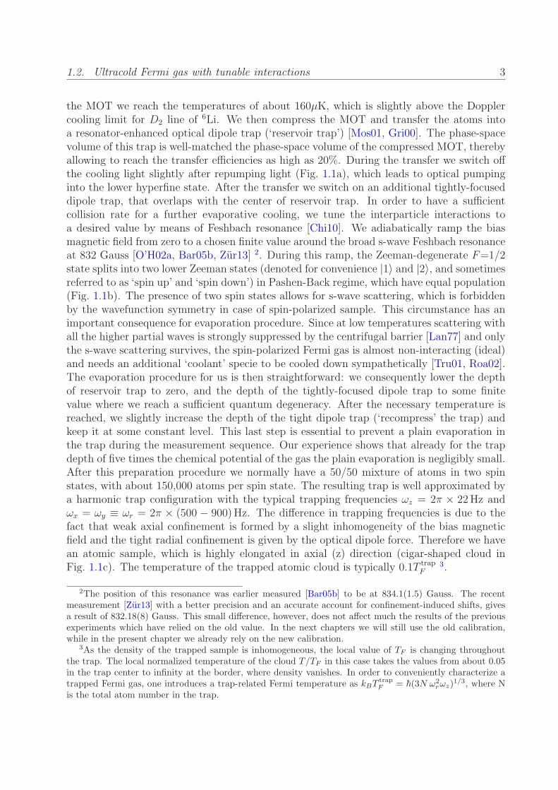
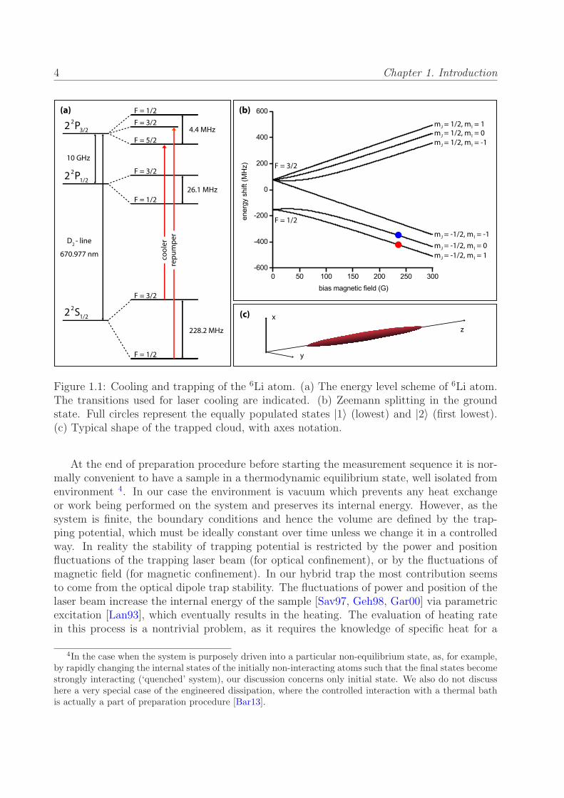
the MOT we reach the temperatures of about 160µK, which is slightly above the Dopplercooling limit for D2 line of 6Li. We then compress the MOT and transfer the atoms intoa resonator-enhanced optical dipole trap (‘reservoir trap’) [Mos01, Gri00]. The phase-spacevolume of this trap is well-matched the phase-space volume of the compressed MOT, therebyallowing to reach the transfer efficiencies as high as 20%. During the transfer we switch offthe cooling light slightly after repumping light (Fig. 1.1a), which leads to optical pumpinginto the lower hyperfine state. After the transfer we switch on an additional tightly-focuseddipole trap, that overlaps with the center of reservoir trap. In order to have a sufficientcollision rate for a further evaporative cooling, we tune the interparticle interactions toa desired value by means of Feshbach resonance [Chi10]. We adiabatically ramp the biasmagnetic field from zero to a chosen finite value around the broad s-wave Feshbach resonanceat 832 Gauss [O’H02a, Bar05b, Zur13] 2. During this ramp, the Zeeman-degenerate F=1/2state splits into two lower Zeeman states (denoted for convenience |1〉 and |2〉, and sometimesreferred to as ‘spin up’ and ‘spin down’) in Pashen-Back regime, which have equal population(Fig. 1.1b). The presence of two spin states allows for s-wave scattering, which is forbiddenby the wavefunction symmetry in case of spin-polarized sample. This circumstance has animportant consequence for evaporation procedure. Since at low temperatures scattering withall the higher partial waves is strongly suppressed by the centrifugal barrier [Lan77] and onlythe s-wave scattering survives, the spin-polarized Fermi gas is almost non-interacting (ideal)and needs an additional ‘coolant’ specie to be cooled down sympathetically [Tru01, Roa02].The evaporation procedure for us is then straightforward: we consequently lower the depthof reservoir trap to zero, and the depth of the tightly-focused dipole trap to some finitevalue where we reach a sufficient quantum degeneracy. After the necessary temperature isreached, we slightly increase the depth of the tight dipole trap (‘recompress’ the trap) andkeep it at some constant level. This last step is essential to prevent a plain evaporation inthe trap during the measurement sequence. Our experience shows that already for the trapdepth of five times the chemical potential of the gas the plain evaporation is negligibly small.After this preparation procedure we normally have a 50/50 mixture of atoms in two spinstates, with about 150,000 atoms per spin state. The resulting trap is well approximated bya harmonic trap configuration with the typical trapping frequencies ωz = 2π × 22Hz andωx = ωy ≡ ωr = 2π × (500 − 900)Hz. The difference in trapping frequencies is due to thefact that weak axial confinement is formed by a slight inhomogeneity of the bias magneticfield and the tight radial confinement is given by the optical dipole force. Therefore we havean atomic sample, which is highly elongated in axial (z) direction (cigar-shaped cloud inFig. 1.1c). The temperature of the trapped atomic cloud is typically 0.1T trap
F3.
2The position of this resonance was earlier measured [Bar05b] to be at 834.1(1.5) Gauss. The recentmeasurement [Zur13] with a better precision and an accurate account for confinement-induced shifts, givesa result of 832.18(8) Gauss. This small difference, however, does not affect much the results of the previousexperiments which have relied on the old value. In the next chapters we will still use the old calibration,while in the present chapter we already rely on the new calibration.
3As the density of the trapped sample is inhomogeneous, the local value of TF is changing throughoutthe trap. The local normalized temperature of the cloud T/TF in this case takes the values from about 0.05in the trap center to infinity at the border, where density vanishes. In order to conveniently characterize atrapped Fermi gas, one introduces a trap-related Fermi temperature as kBT
trapF = ~(3N ω2
rωz)1/3, where N
is the total atom number in the trap.
4 Chapter 1. Introduction
2 P3/22
2 P1/22
2 S1/22
10 GHzF = 3/2
F = 1/2F = 3/2
F = 5/2
F = 1/2
F = 3/2
F = 1/2
cool
erre
pum
per
4.4 MHz
26.1 MHz
228.2 MHz
D - line2
670.977 nm
z
y
x
F = 3/2
F = 1/2
m = -1/2, m = 0J I
m = -1/2, m = -1J I
m = 1/2, m = -1J I
m = 1/2, m = 0J I
m = 1/2, m = 1J I
m = -1/2, m = 1J I
(a)
(c)
(b)
Figure 1.1: Cooling and trapping of the 6Li atom. (a) The energy level scheme of 6Li atom.The transitions used for laser cooling are indicated. (b) Zeemann splitting in the groundstate. Full circles represent the equally populated states |1〉 (lowest) and |2〉 (first lowest).(c) Typical shape of the trapped cloud, with axes notation.
At the end of preparation procedure before starting the measurement sequence it is nor-mally convenient to have a sample in a thermodynamic equilibrium state, well isolated fromenvironment 4. In our case the environment is vacuum which prevents any heat exchangeor work being performed on the system and preserves its internal energy. However, as thesystem is finite, the boundary conditions and hence the volume are defined by the trap-ping potential, which must be ideally constant over time unless we change it in a controlledway. In reality the stability of trapping potential is restricted by the power and positionfluctuations of the trapping laser beam (for optical confinement), or by the fluctuations ofmagnetic field (for magnetic confinement). In our hybrid trap the most contribution seemsto come from the optical dipole trap stability. The fluctuations of power and position of thelaser beam increase the internal energy of the sample [Sav97, Geh98, Gar00] via parametricexcitation [Lan93], which eventually results in the heating. The evaluation of heating ratein this process is a nontrivial problem, as it requires the knowledge of specific heat for a
4In the case when the system is purposely driven into a particular non-equilibrium state, as, for example,by rapidly changing the internal states of the initially non-interacting atoms such that the final states becomestrongly interacting (‘quenched’ system), our discussion concerns only initial state. We also do not discusshere a very special case of the engineered dissipation, where the controlled interaction with a thermal bathis actually a part of preparation procedure [Bar13].
1.2. Ultracold Fermi gas with tunable interactions 5
particular trapping configuration [Bul05]. The typical measured heating rates in our experi-ment are of about 0.01-0.02 T trap
F per second at the temperatures of 0.1T trapF , which gives on
the timescales of the actual measurements (about 50-200 ms) the increase of the tempera-ture only by a few percent. We can be therefore confident that the temperature and otherthermodynamic quantities which we measure at some time moment during the experiment,are well defined for the whole experimental sequence and the state of the system is a verygood approximation to global equilibrium one.
1.2.2 Tuning the interactions
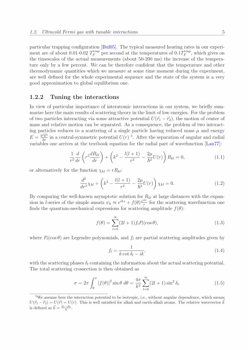
In view of particular importance of interatomic interactions in our system, we briefly sum-marize here the main results of scattering theory in the limit of low energies. For the problemof two particles interacting via some attractive potential U(~r1 − ~r2), the motion of center ofmass and relative motion can be separated. As a consequence, the problem of two interact-ing particles reduces to a scattering of a single particle having reduced mass µ and energy
E = ~2~k2
2µin a central-symmetric potential U(r) 5. After the separation of angular and radial
variables one arrives at the textbook equation for the radial part of wavefunction [Lan77]:
1
r2d
dr
(
r2dRkl
dr
)
+
(
k2 − l(l + 1)
r2− 2µ
~2U(r)
)
Rkl = 0, (1.1)
or alternatively for the function χkl = rRkl:
d2
dr2χkl +
(
k2 − l(l + 1)
r2− 2µ
~2U(r)
)
χkl = 0. (1.2)
By comparing the well-known asymptotic solution for Rkl at large distances with the expan-sion in l-series of the simple ansatz ψk ≈ eikz + f(θ) e
ikr
rfor the scattering wavefunction one
finds the quantum-mechanical expressions for scattering amplitude f(θ):
f(θ) =∞∑
l=0
(2l + 1)flPl(cos θ), (1.3)
where Pl(cos θ) are Legendre polynomials, and fl are partial scattering amplitudes given by
fl =1
k cot δl − ik, (1.4)
with the scattering phases δl containing the information about the actual scattering potential.The total scattering crossection is then obtained as
σ = 2π
∫ π
0
|f(θ)|2 sin θ dθ = 4π
k2
∞∑
l=0
(2l + 1) sin2 δl. (1.5)
5We assume here the interaction potential to be isotropic, i.e., without angular dependence, which meansU(~r1 − ~r2) = U(~r) = U(r). This is well satisfied for alkali and earth-alkali atoms. The relative wavevector ~k
is defined as ~k = ~p1−~p2
~.

6 Chapter 1. Introduction
Therefore, in order to calculate the full crossection for some arbitrary value of the energy k2
one needs to know all the partial-wave contributions. The situation is however dramaticallysimplified for the scattering in the limit of very low energies 6. Here, the scattering phases δldepend on the energy as ∝ k2l [Lan77]. All the contributions from partial waves with l ≥ 1become negligibly small, and in the limit of k → 0 the scattering is completely defined by asingle parameter - the s-wave (l = 0) scattering length a:
limk→0
f0 = −a (1.6)
The s-wave scattering phase is then expressed as δ0 = −ka. We note that to properly accountfor the energy dependence of scattering one has to calculate the correction to the scatteringphase by Taylor expansion of k cot δ0 in Eq. 1.4 as k cot δ0 = − 1
a+ 1
2k2re+ . . . ≡ − 1
a(k), where
re is so-called effective range of the potential (see, for instance, [Koh06]). For the purposesof further explanation, we can safely neglect this small correction.
To understand the main properties of the s-wave scattering length a and the originof scattering resonances it is enough to consider a spherical square well model potential(Fig. 1.2a) [Gio08, Wal08]. In such a system the resonance in scattering as a function ofpotential depth is expected to occur whenever the potential is able to support one morebound state. From the mathematical point of view, one solves the equation for the radialwavefunctuion χ(r) (Eq. 1.2) in the full range 0 < r < ∞ for E = ~
2k2
2µ> 0 continuum
scattering states and takes the limit of k → +0. Analogously, one finds a bound-statesolution with E = −~
2κ2
2µ< 0 and takes the limit of κ → −0. Then, these solutions have to
be connected at the point E = 0. By doing so, one obtains the scattering resonances in theform of Eq. 1.7 and the universal 7 bound state energy (Eq. 1.8).
a = r0
(
1− tan(κ0r0)
κ0r0
)
, (1.7)
where κ0 is defined via depth of the well U0 =~2κ2
0
2µ,
Eb =~2
2µa2. (1.8)
From the physical point of view, the scattering resonance occurs exactly when the energyof the bound state coincides with the scattering energy of the ‘free particle’. For a realatomic system, it is not easy to fine-tune the depth of the interaction potential (especially in
situ) in order to bring its bound state very close to threshold. However, if we consider the
6The ‘low energies’ in this case are defined by condition kr0 ≪ 1. In other words, the de Brogliewavelength λdB of the particle becomes much larger than the range of potential. This is normally the casein ultracold gases if the particles interact via short-range Van der Waals potentials U(r) = −C6
r6 . For Liatoms, r0 ∼= rV dW ≈ 30a0 and λdB ≈ 1.35 · 104a0 at 1µK, where a0 is Bohr radius. The limit of k → 0 isfrequently a good approximation to describe low-energy scattering physics.
7The radial wavefunction of these near-threshold ‘halo dimer’ bound state is well approximated as R(r) ∼=1√2π a
e−r/a
r . The average separation between the atoms is then a/2 [Koh06], which means that practically
all the wavefunction is outside the range of potential. The fine details of potential are thus irrelevant for thescattering, or, in other words, the scattering is universal. This holds as long as a ≫ r0.
1.2. Ultracold Fermi gas with tunable interactions 7
r
0
E
E
0 r r 0 VdW0 r
0
E
0 r
E
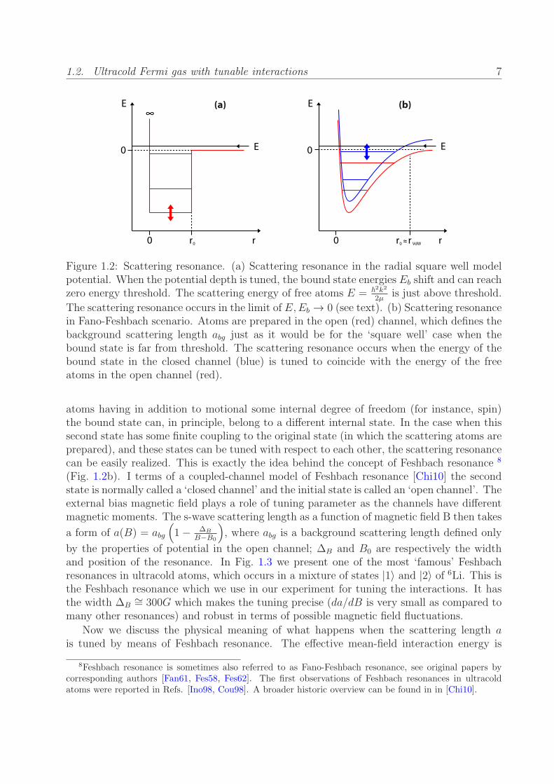
(a) (b)
Figure 1.2: Scattering resonance. (a) Scattering resonance in the radial square well modelpotential. When the potential depth is tuned, the bound state energies Eb shift and can reachzero energy threshold. The scattering energy of free atoms E = ~
2k2
2µis just above threshold.
The scattering resonance occurs in the limit of E,Eb → 0 (see text). (b) Scattering resonancein Fano-Feshbach scenario. Atoms are prepared in the open (red) channel, which defines thebackground scattering length abg just as it would be for the ‘square well’ case when thebound state is far from threshold. The scattering resonance occurs when the energy of thebound state in the closed channel (blue) is tuned to coincide with the energy of the freeatoms in the open channel (red).
atoms having in addition to motional some internal degree of freedom (for instance, spin)the bound state can, in principle, belong to a different internal state. In the case when thissecond state has some finite coupling to the original state (in which the scattering atoms areprepared), and these states can be tuned with respect to each other, the scattering resonancecan be easily realized. This is exactly the idea behind the concept of Feshbach resonance 8
(Fig. 1.2b). I terms of a coupled-channel model of Feshbach resonance [Chi10] the secondstate is normally called a ‘closed channel’ and the initial state is called an ‘open channel’. Theexternal bias magnetic field plays a role of tuning parameter as the channels have differentmagnetic moments. The s-wave scattering length as a function of magnetic field B then takes
a form of a(B) = abg
(
1− ∆B
B−B0
)
, where abg is a background scattering length defined only
by the properties of potential in the open channel; ∆B and B0 are respectively the widthand position of the resonance. In Fig. 1.3 we present one of the most ‘famous’ Feshbachresonances in ultracold atoms, which occurs in a mixture of states |1〉 and |2〉 of 6Li. This isthe Feshbach resonance which we use in our experiment for tuning the interactions. It hasthe width ∆B
∼= 300G which makes the tuning precise (da/dB is very small as compared tomany other resonances) and robust in terms of possible magnetic field fluctuations.
Now we discuss the physical meaning of what happens when the scattering length ais tuned by means of Feshbach resonance. The effective mean-field interaction energy is
8Feshbach resonance is sometimes also referred to as Fano-Feshbach resonance, see original papers bycorresponding authors [Fan61, Fes58, Fes62]. The first observations of Feshbach resonances in ultracoldatoms were reported in Refs. [Ino98, Cou98]. A broader historic overview can be found in in [Chi10].
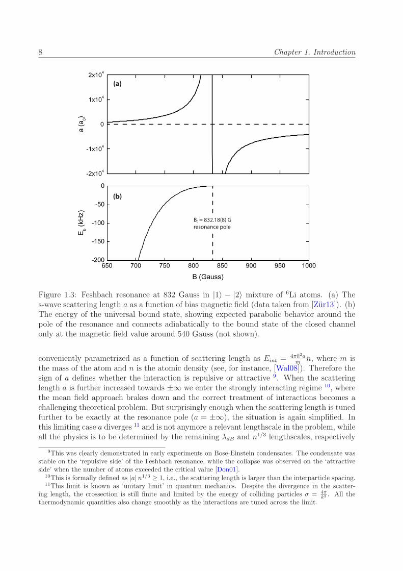
8 Chapter 1. Introduction
B = 832.18(8) Gresonance pole
0
(a)
(b)
Figure 1.3: Feshbach resonance at 832 Gauss in |1〉 − |2〉 mixture of 6Li atoms. (a) Thes-wave scattering length a as a function of bias magnetic field (data taken from [Zur13]). (b)The energy of the universal bound state, showing expected parabolic behavior around thepole of the resonance and connects adiabatically to the bound state of the closed channelonly at the magnetic field value around 540 Gauss (not shown).
conveniently parametrized as a function of scattering length as Eint =4π~2am
n, where m isthe mass of the atom and n is the atomic density (see, for instance, [Wal08]). Therefore thesign of a defines whether the interaction is repulsive or attractive 9. When the scatteringlength a is further increased towards ±∞ we enter the strongly interacting regime 10, wherethe mean field approach brakes down and the correct treatment of interactions becomes achallenging theoretical problem. But surprisingly enough when the scattering length is tunedfurther to be exactly at the resonance pole (a = ±∞), the situation is again simplified. Inthis limiting case a diverges 11 and is not anymore a relevant lengthscale in the problem, whileall the physics is to be determined by the remaining λdB and n1/3 lengthscales, respectively
9This was clearly demonstrated in early experiments on Bose-Einstein condensates. The condensate wasstable on the ‘repulsive side’ of the Feshbach resonance, while the collapse was observed on the ‘attractiveside’ when the number of atoms exceeded the critical value [Don01].
10This is formally defined as |a|n1/3 ≥ 1, i.e., the scattering length is larger than the interparticle spacing.11This limit is known as ‘unitary limit’ in quantum mechanics. Despite the divergence in the scatter-
ing length, the crossection is still finite and limited by the energy of colliding particles σ = 4πk2 . All the
thermodynamic quantities also change smoothly as the interactions are tuned across the limit.
1.3. BEC-BCS crossover 9
associated with temperature and density. This lengthscales argument, lies in the heart of so-called ‘universal hypothesis’ [Ho04]. From the thermodynamical point of view, even thoughthe interactions are strongest allowed by quantum mechanics, they do not enter explicitlyinto any thermodynamic quantity and eventually just lead to ‘rescaling’ of the correspondingideal gas quantities. The physics in this regime is independent on the details of interactionpotential (as discussed above) and hence on the type of the interacting particles. Unitarygas can be in principle realized for both bosons and fermions. However, the unitary Bose gasis unstable against molecule-molecule and molecule-atom collisions [Xu03, Web03, Rem12].In the fermionic mixture of two spin state, the three-body decay is strongly suppressed byPauli principle (see [Pet04] and references therein). This makes our system well suitable forstudying the many-body physics in the strongly interacting regime and, in particular, in theunitary limit.
1.3 BEC-BCS crossover
In this section we discuss the rich physics of the so-called ‘BEC-BCS crossover’ which takesplace in the Fermi gas as the interparticle interactions are tuned across the Feshbach reso-nance. The purpose here is not to give a detailed review of strongly interacting Fermi gases,but rather to provide a necessary minimum to understand the physics of the system and ourmotivation for experiments presented in the following chapters. After introducing the phasediagram, we overview the experimental methods used so far to study the properties of theFermi gas in BEC-BCS crossover and the main achievements these methods have lead to. Inthis general context, we consider the advantages and limitations of the methods used in ourexperiment. Finally, we discuss a number of ‘extensions’ to this model BEC-BCS crossoversystem, which allow to address new physics.
1.3.1 Phase diagram
Here we introduce step by step the phase diagram (Fig. 1.4) of the system described in theprevious section, namely a degenerate Fermi gas in a balanced mixture of two spin stateswith resonantly enhanced interactions, confined in a harmonic trap. Phases are shown asa function of reduced temperature T/T trap
F and interaction strength which is convenientlyparametrized by dimensionless interaction parameter 1/kFa. The Fermi wavevector kF isrelated here to the temperature T trap
F , and the region of −1 < 1/kFa < 1 represents thereforean effectively strongly interacting regime for the trapped Fermi gas. Two well-understoodlimits on the interaction axis are 1/kFa→ ±∞. They correspond to the small repulsive andsmall attractive effective mean-field interaction. On the positive side of Feshbach resonancethe molecular bound state exists. Therefore, a pair of fermions with opposite spins can forma molecule and, if the temperature is low enough, these composite molecules condense. Thisis the BEC-limit (left side on the phase diagram). On the opposite side of the Feshbachresonance, there is no bound state and the pairing is essentially many-body effect occurringvia BCS-scenario, analogously to the pairing between electrons in metallic superconductor.This is a BCS-limit (right side on the phase diagram). The easiest way to connect these two
10 Chapter 1. Introduction
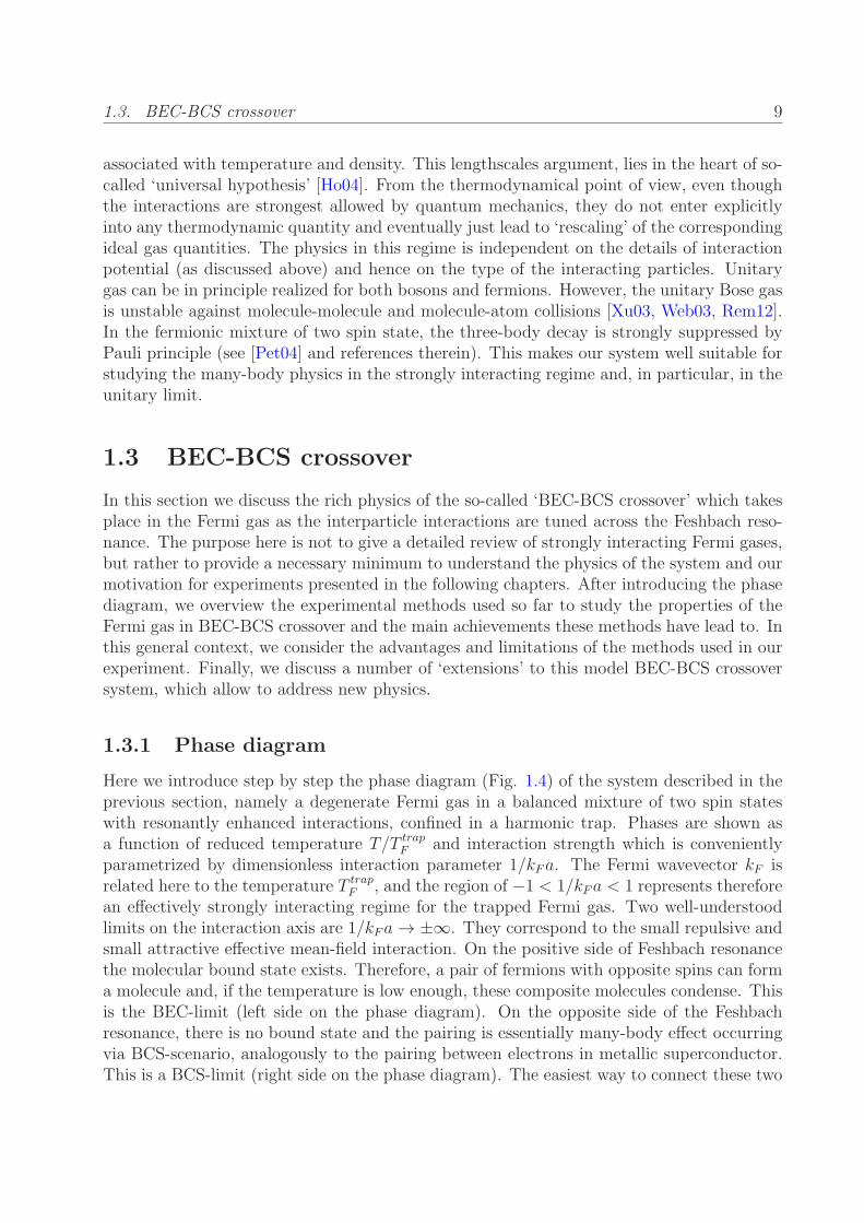
TTc
*
normal gasno pairingpairing,
no condensate
BEC BCS
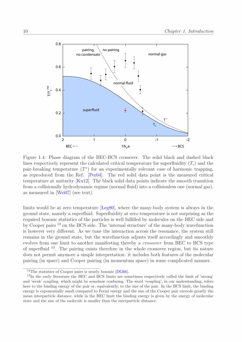
Figure 1.4: Phase diagram of the BEC-BCS crossover. The solid black and dashed blacklines respectively represent the calculated critical temperature for superfluidity (Tc) and thepair-breaking temperature (T ∗) for an experimentally relevant case of harmonic trapping,as reproduced from the Ref. [Per04]. The red solid data point is the measured criticaltemperature at unitarity [Ku12]. The black solid data points indicate the smooth transitionfrom a collisionally hydrodynamic regime (normal fluid) into a collisionless one (normal gas),as measured in [Wri07] (see text).
limits would be at zero temperature [Leg80], where the many-body system is always in theground state, namely a superfluid. Superfluidity at zero temperature is not surprising as therequired bosonic statistics of the particles is well fulfilled by molecules on the BEC side andby Cooper pairs 12 on the BCS side. The ‘internal structure’ of the many-body wavefunctionis however very different. As we tune the interaction across the resonance, the system stillremains in the ground state, but the wavefunction adjusts itself accordingly and smoothlyevolves from one limit to another manifesting thereby a crossover from BEC to BCS typeof superfluid 13. The pairing exists therefore in the whole crossover region, but its naturedoes not permit anymore a simple interpretation: it includes both features of the molecularpairing (in space) and Cooper pairing (in momentum space) in some complicated manner.
12The statistics of Cooper pairs is nearly bosonic [DG66].13In the early literature the BEC and BCS limits are sometimes respectively called the limit of ‘strong’
and ‘weak’ coupling, which might be somehow confusing. The word ‘coupling’, in our understanding, refershere to the binding energy of the pair or, equivalently, to the size of the pair. In the BCS limit, the bindingenergy is exponentially small compared to Fermi energy and the size of the Cooper pair exceeds greatly themean interparticle distance, while in the BEC limit the binding energy is given by the energy of molecularstate and the size of the molecule is smaller than the interparticle distance.

1.3. BEC-BCS crossover 11
If we consider now to increase the temperature, more and more excitations above theground state are created and at some point the system undergoes a second order phase tran-sition into a normal state. As we can see, this happens already at very low temperatures onthe BCS side. For this matter the knowledge on the critical temperature for superfluidity(Tc line in Fig. 1.4) is essential to understand the crossover regime at finite temperatures 14.The crossover theory is now rigorously generalized and includes the region of finite tempera-tures [Noz85, Per04]. A question of pairing could be also addressed in the finite-temperatureregion. In Fig. 1.4 we show the ‘critical temperature’ for pairing (T ∗ line) which is alwaysabove the critical temperature for superfluidity Tc. The region between two curves, wherethere are already preformed pairs but no superfluidity, is still not well understood. Thisregion is called ‘pseudogap regime’ [Che05, Tsu10] in analogy to the corresponding regionin HTSs.
Now, as the two limits are connected in the whole diagram, we note that the most ofcrossover evolution happens in the region of strong interactions [Noz85] and ‘zoom’ into thisregion. Considerable efforts have been already made to understand the strongly interactingFermi system [Ing08, Gio08], still the theoretical description remains a challenging problemdue to its non-perturbative nature. Here we discuss a few important consequences imposedby the strong interactions, which will be the focus of the research presented in the nextchapters.
In the strongly interacting regime the phenomenon of superfluidity has to be clearlydistinguished from the pair condensation (see, for example, [Fuk07c]) even at the lowesttemperatures (zero temperature in theory). In a very weakly interacting BEC, the densityof the condensate (occupation of the k = 0 state) is almost equal to the superfluid den-sity [Pit03], while for a strongly interacting BEC the condensate density is expected to bedepleted [Lan80b]. This was also demonstrated in the experiments on superfluid helium,where the condensate fraction was determined precisely [Gly00]. In Chapter 2, we real-ize a truly strongly interacting molecular BEC and experimentally address the question ofcondensation.
Strength of the interactions also affects the collective response properties of the system,namely whether its dynamic behavior is more like the one of a fluid (hydrodynamic) or ofa gas (collisionless). While the superfluid is always hydrodynamic, the transition region innormal state is indicated by the black filled data points in Fig. 1.4. The criterion is howeverquantitative: one compares the collision rate ν and the characteristic motional timescale,which is given by trapping frequency ω. If ν ≫ ω, then the local equilibrium is easilyestablished, which is a characteristic of liquid. If the opposite limit ν ≪ ω holds, then theatoms practically ‘don’t see’ each other and the system is similar to an ideal gas. With thesedefinition the transition boundary is rather smooth in reality and depends on the value oftrapping frequencies 15. In Fig. 1.4 we define the hydrodynamic region with respect to thefast radial degree of freedom (see Fig. 1.1c), with a typical trap frequency ωr ≈ 1 kHz. In
14The dependence of the critical temperature Tc on interaction is qualitatively different for a case ofhomogeneous system [Per04].
15Using a very elongated trap with an aspect ratio ωr/ωz∼= 100 it is possible to reach a hydrodynamic be-
havior along the z-axis, while being collisionless in radial direction. This might be of considerable advantage,when the attainable interaction strength is restricted [Mep09a].

12 Chapter 1. Introduction
Chapters 3 and 4, we approach the superfluid-to-normal hydrodynamic transition, which waspractically indistinguishable before in related experiments, with a new sensitive method.
The unitary limit of interactions (1/kFa = 0 in Fig. 1.4) needs a special treatment. Aswe have mentioned earlier, the universality hypothesis significantly simplifies the descriptionof the system [Hau07, Hau08, Hu07] which leads to the maximum ‘overlap’ between thetheory and experiment in strongly interacting regime to be reached at unitarity. One of therecent achievement was to precisely measure the equation of state and the critical temper-ature for superfluidity [Ku12]. In Chapter 5, we measure at the first time the superfluiddensity in the resonantly interacting Fermi gas as a function of temperature - a quantity offundamental importance. The particular ‘magic’ of the superfluid density, in our opinion, isthat it is indeed the quantity which bridges the microscopic and macroscopic worlds in ourmany-body system. Microscopic relation is established via the spectrum of the elementaryexcitations, which affects the superfluid density in the integral sense [Lan80a]. The rela-tion to the macroscopic world is due to the fact that superfluid density directly affects thethermodynamics and hydrodynamics of the many-body system.
1.3.2 Experimental methods
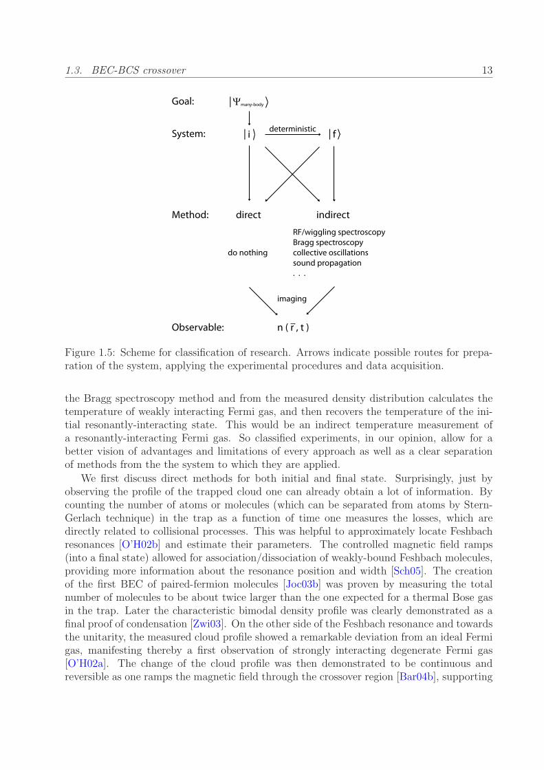
We classify now the research in the BEC-BCS crossover from methodological point of viewusing a very general and simple scheme represented in Fig. 1.5. The main goal of research is tounderstand the properties of many-body system, which we formally depicted as |Ψmany−body〉.To study these properties, one prepares the system in initial state |i〉, which corresponds tosome point on the phase diagram (Fig. 1.4), and wants to measure on it. There are twopossibilities from here: either to immediately perform the measurement on the initial state,or to deterministically change the initial state into final state |f〉 and measure on the finalstate as it might be easier for some reason. Deterministic change is crucial to preciselyrecover afterwards the properties of initial state from the final-state measurement. One canthen apply different methods to study either of two states. We classify them as ‘direct’,which means practically doing nothing to a system and go directly to data acquisition, and‘indirect’ which implies some experimental procedures before the data acquisition. Althoughthis separation might look a bit strange, we find it to well reflect the actual situation andhelpful to avoid semantic confusion. Data acquisition means normally the imaging of thecloud. The measured quantity is always the density as a function of position and time n(~r, t)or, more precisely, its integral along the imaging direction. From these data, depending onimaging techniques and parameters, one is able to recover the important quantities (like,for example, equilibrium density n(~r) or momentum n(~p) distributions in the trapped cloud,total number of atoms N or its time dependence N(t)), and conclude on the properties ofthe many-body state.
For example, in a hypothetical experiment one prepares a weakly interacting Fermi gas inthe BCS limit, performs an absorption time-of-flight imaging, reconstructs the initial in-trapmomentum distribution function and derives from it the temperature of the gas. This wouldbe a direct temperature measurement of a weakly-attractive Fermi gas. In another hypo-thetical experiment, one prepares a resonantly-interacting Fermi gas, adiabatically rampsthe magnetic field towards the BCS side where the first experiment was performed, applies
1.3. BEC-BCS crossover 13
|
i
many-body
| f|
direct indirect
deterministic
do nothing
RF/wiggling spectroscopyBragg spectroscopycollective oscillationssound propagation. . .
n ( r , t )
Method:
System:
Goal:
imaging
Observable:
Figure 1.5: Scheme for classification of research. Arrows indicate possible routes for prepa-ration of the system, applying the experimental procedures and data acquisition.
the Bragg spectroscopy method and from the measured density distribution calculates thetemperature of weakly interacting Fermi gas, and then recovers the temperature of the ini-tial resonantly-interacting state. This would be an indirect temperature measurement ofa resonantly-interacting Fermi gas. So classified experiments, in our opinion, allow for abetter vision of advantages and limitations of every approach as well as a clear separationof methods from the the system to which they are applied.
We first discuss direct methods for both initial and final state. Surprisingly, just byobserving the profile of the trapped cloud one can already obtain a lot of information. Bycounting the number of atoms or molecules (which can be separated from atoms by Stern-Gerlach technique) in the trap as a function of time one measures the losses, which aredirectly related to collisional processes. This was helpful to approximately locate Feshbachresonances [O’H02b] and estimate their parameters. The controlled magnetic field ramps(into a final state) allowed for association/dissociation of weakly-bound Feshbach molecules,providing more information about the resonance position and width [Sch05]. The creationof the first BEC of paired-fermion molecules [Joc03b] was proven by measuring the totalnumber of molecules to be about twice larger than the one expected for a thermal Bose gasin the trap. Later the characteristic bimodal density profile was clearly demonstrated as afinal proof of condensation [Zwi03]. On the other side of the Feshbach resonance and towardsthe unitarity, the measured cloud profile showed a remarkable deviation from an ideal Fermigas, manifesting thereby a first observation of strongly interacting degenerate Fermi gas[O’H02a]. The change of the cloud profile was then demonstrated to be continuous andreversible as one ramps the magnetic field through the crossover region [Bar04b], supporting
14 Chapter 1. Introduction
the idea of a smooth evolution.
Based on understanding of the atomic profiles on the BEC side, it has become possibleto show a condensate of pairs to exist in the strongly interacting regime [Reg04, Zwi04] by‘projecting’ the corresponding many-body wavefunction onto a relatively well-known molec-ular BEC wavefunction by means of fast magnetic field ramp. Completely analogous to thequantum-mechanical textbook state projection, this procedure shows the condensate fractionin the final state (BEC) which must be the one present in initial state. Technical limitationsof experiments, however, don’t allow for a perfect projection and there seems to be some‘evolution’ admixture still present during the ramp. The errors are relatively difficult toquantify and, in our opinion, some independent measurements are needed to validate (orrefute) this projection procedure 16.
The phenomenon of superfluidity was unambiguously demonstrated by creation of vor-tices in a rotating Fermi gas (final state) [Zwi05], in analogy to earlier experiments on atomicBECs. Later, the predicted signature of superfluid-to-normal transition was revealed in thetrapped cloud’s density profile [Zwi06a]. In our opinion, this was the first experiment, wherethe presence of the trap turned out a rather great advantage than just something unavoid-able. Very recent experiments have directly demonstrated the key property of superfluidstate, namely a frictionless flow (the drop of resistance to zero) in the resonantly interactingFermi gas, with a carefully engineered confinement potential [Sta12].
The studies of thermodynamics in the strongly interacting state was particularly fruitfulin the unitarity-limited case. Of considerable importance in this sense was the measurementof specific heat capacity [Kin05b] and formulation of the virial theorem for a trapped gas[Tho05], which gave a direct access to the energy of the system and favored the first mea-surements of the equation of state (EOS) at unitarity [Luo07, Hor10]. These measurementsrelied on thermometry performed in a final state, after an expectedly adiabatic ramp ofmagnetic field. The adiabaticity of the ramp, however, was not satisfied very well, givingrise to relatively large errors in temperature calibration and in the whole measured EOS.Recent measurements on the EOS were performed with a significantly better thermometry[Nas10, Nav10], or even without a need to measure the temperature [Ku12]. These ex-periments have used directly a specific property of harmonic trapping potential [Ho10] 17
and developed very elegant approaches to measure the EOS. The experiment of MIT group[Ku12] was able to measure the Bertsch parameter ξ and the critical temperature Tc of aunitary Fermi gas with an impressive precision.
Now we discuss the indirect methods, which were applied so far to study the BEC-BCScrossover. Several spectroscopic methods were used to understand the actual ‘structure’ ofthe many-body wavefunction and the origins of pairing.
RF spectroscopy [Mar88] tool was first applied to fermions [Reg03a, Gup03] to measure
16Recently, we extended the idea of interference experiments [Cas97] from weakly-interacting atomic tostrongly interacting molecular condensates (Chapter 2). We found that strong interactions tend to smearout the interference pattern and prevent the interpenetration of two clouds thereby prohibiting the study inthe most interesting regime around unitarity. As a conclusion, there could be made no direct comparisonbetween our experiment and the above-mentioned ones.
17In our opinion, this is a very rare case when the usefulness of theoretical work for experiments can behardly overestimated.

1.3. BEC-BCS crossover 15
the mean-field interaction shifts and map the scattering length as a function of magneticfield near Feshbach resonance. Later, the binding energy of the universal dimer was usedto precisely characterize Feshbach resonance [Reg03b, Bar05b]. The presence of pairing wasobserved in the whole strongly interacting regime [Chi04] as the gap in RF-spectra (‘pairinggap’, ∆). The pairing gap was shown to have a meaning of molecular binding energy on theBEC side of the resonance. Further experiments extended the pairing gap measurement tobe tomographic in the trap [Shi07], and presented the measurement of the pair size [Sch08]with an experimental scheme that minimized the final-state-induced shifts. The ‘wiggling’method based on the rf-modulation of the bias magnetic field [Gre05] was used for similarexperiments, and demonstrated some advantages over the conventional rf spectroscopy.
The photo emission spectroscopy showed a possibility to resolve momentum in the rf-spectra and allowed for measurement of quasiparticle dispersion curve [Ste08, Gae10, Che09].
The optical molecular spectroscopy distinguished between free atoms and paired atoms onboth sides of the Feshbach resonance [Par05], measuring hereby a closed-channel contributioninto the universal bound state on molecular side. This experiment also referred to thesuperfluid order parameter (‘superfluid gap’, which is also denoted ∆ and strictly speakingcoincides with a pairing gap only in the BCS limit), however, the role played by the non-condensed pairs was not clear from measurements.
Bragg spectroscopy proved itself a powerful tool to investigate the pairing-related phe-nomena in BEC-BCS crossover [Vee08]. The distinction between pairs and atoms is donehere by mass difference rather than by energy shifts like in rf spectroscopy. A large trans-ferred momentum of the order of kF allowed for sensitive study of the two-body correlations(at the corresponding distances of the order of 1/kF ) via measuring the dynamic structurefactor [Pin66, Com06], even in the strongly interacting regime. Further studies establisheda connection between pair correlations and the universal contact [Kuh11, Tan08a, Tan08c,Tan08b]. A method in some sense similar to the Bragg spectroscopy - a drag by movinglattice (implemented for bosons earlier: [DS05]) - was used to measure the critical velocityfor superfluidity in the whole crossover [Mil07].
We will discuss now in some more details the methods employed in experiments pre-sented in the last three chapters, namely the method of collective oscillations and the soundpropagation.
The method of collective oscillations has been first used for atomic BECs [Pit03], andlater applied to strongly interacting Fermi gases [Gio08]. It is based on a simple considerationthat if we mechanically perturb a whole bulk of the fluid or gas about its equilibrium state,we excite a collective motion of the whole system in which the dynamics would be defined bythe equilibrium properties. The crucial property of these collective oscillations is that theyare normally long-lived. One is able to observe many oscillation periods and hereby definethe relevant oscillation frequency and damping constant with a high precision. The simplestmodes (sloshing modes) are useful to accurately characterize the trap (by measuring trappingfrequencies), which is now the standard technique. Collective oscillation which affect the den-sity of the cloud (compression modes) are sensitive to the EOS of a system. The experimentson compression modes accessed the superfluid EOS in the whole crossover [Bar04a, Kin04a].Later measurements on radial compression mode provided crossover EOS with a much betterprecision, and facilitated a direct comparison to the zero-temperature predictions [Hei04].

16 Chapter 1. Introduction
The small beyond-mean-field correction, known as LHY correction [Lee57], was revealed forthe BEC equation of state. The above-mentioned experiments also showed the signaturesof transition from hydrodynamic to collisionless regime, which were studied later in moredetail with surface modes [Alt07c, Wri07]. Our recent experiments on collective modes ap-proached the EOS of the unitary Fermi gas along the temperature axis, and proved beingsensitive to the interaction effects across the superfluid phase transition (Chapters 3 and 4).An interesting way to measure via collective modes the critical temperature for superfluiditywas presented by study of radial quadrupole mode in a rotating gas (final state) [Rie11].
In contrast to the method of collective oscillations, the experiments on propagation ofthe density perturbation (sound wave) did not show a great potential for precision tests ofthe EOS. Clearly, the speed of sound depends on the thermodynamics of the trapped gas.The density pulse being normally excited in the center of the cigar-shaped cloud, propagatestowards the boundary and eventually disappears. The quantity extracted is the speed ofsound, which does not have that high accuracy as the collective mode frequency (betterthan 1%). Therefore, the earlier measurements on the sound propagation were more ofa proof-of-principle type [Jos07] and followed the similar measurements done with atomicBECs [And97a], still demonstrating a very good agreement with an expectation from EOSresults [Cap06]. One difficulty of the experiment of this type is the following. On one hand,to relatively well define the position of a propagating pulse, one needs a good signal-to-noiseratio, i.e., the deeper (higher) is the well (hill) - the better. On the other hand, the stronger isthe propagating excitation, the less accurately it can be considered as a perturbation. Morequantitatively, when the depth of the well becomes of the order of chemical potential in thecenter of the trap, this is not a perturbation anymore and the necessary corrections neededto be introduced into calculations, if not the whole concept to be changed. In this case, acompromise has to be found and the technical limitations like the quality of the imagingsystem matter a lot. Moreover, for the case of a deep well, one faces nonlinearities andsoliton physics [Yef13]. A considerably large attention the sound-propagation experimentsgained because of numerous theoretical paper on possible propagation of second sound wavesin strongly interacting Fermi gases [Hei06, Tay09, Hu10, Ber10] and the experiments relatedto the second sound in BECs [SK98, Mep09b, Mep09a]. The formulation of Landau’s two-fluid hydrodynamics turned out to be exactly applicable to the strongly interacting Fermigases, in the broad region of phase diagram (Fig. 1.4) below the critical temperature whereboth normal and superfluid components exist and are strongly hydrodynamic. Our systemtherefore was proposed as an ideal system in the field of ultracold atoms to observe thesecond sound waves. While the second sound in BECs is simply a Bogoliubov sound (adensity wave propagating in a condensate) [Gri97], the strongly interacting nature of oursystem suggested similarities with superfluid helium and a ‘classical’ concept of second soundas an entropy (or temperature wave). Surprisingly enough, new calculations showed thatthe second sound wave in our system has also a finite variation in the density. We thenmade an effort of inventing a very simple procedure to create a local temperature excitation(essential for coupling to the second sound ansatz [Kha65], but not to the first sound one)and observed the resulting propagation of second sound. We hope that our experimentspresented in the Chapter 5, might stimulate further development of the sound propagationmethod.
1.3. BEC-BCS crossover 17
We would like to note, that the last three methods, the Bragg spectroscopy, collectiveoscillations and sound propagation, have one thing in common: they all probe the densityresponse properties of the many-body system. Therefore, they could be all treated and un-derstood [Hu10] within a very general and well established response theory [Lan80b, Pin66].The question is only about the type, or maybe better - regime of the excitation which wepurposely choose. Can we connect these three methods and understand everything in termsof Bragg spectroscopy, for example? In Bragg spectroscopy, the excitation is done to thewhole cloud and is essentially delocalized in space, but localized in momentum and energy.In the sound propagation experiment, one uses a perturbation which is pretty much local-ized in space that would correspond to a wavepacket in momentum space. The total energytransfer in this case becomes an integral quantity over the momenta of the wavepacket. Thecollective oscillation represents a limiting case of a sound propagation of a very narrow mo-mentum wavepacket, which corresponds to the oscillation of the whole trapped system inreal space. This is the effect of the boundary conditions imposed by the trapping potential,which ‘narrows down’ the momentum width of a sound excitation. This is analogous tothe laser linewidth narrowing by cavity, with a difference that reflection happens not at themirrors in the ends of a cavity, but in the whole harmonic trap as its walls gradually rise.Only the certain waves survive after this distributed reflection to form a collective modein a given trap geometry. From this intuitive arguments we see that perhaps the collectiveoscillations can be approached from Bragg spectroscopy perspective. This is why it makessense to discuss the low-frequency impact, generated by collective modes, in the dynamicstructure factor and density response function which can be revealed in Bragg spectroscopyexperiment [Hu10, Tay07]. For the local density perturbation, propagating through thecloud, the interpretation in terms of Bragg spectroscopy would be problematic. As to ourknowledge, there were no experiments demonstrating the collective-modes impact by Braggspectroscopy and the latter is still ideologically detached from the other two methods usedin our experiment.
1.3.3 Extensions of the crossover physics
Here we list the ‘extensions’ of strongly interacting fermions beyond our model BEC-BCScrossover system based on a balanced two-spin mixture of a single specie. These extensionsare realized via tuning additional parameters, such as balance between population of twospin states or the total number of atoms, creating a mixture of fermions of more than twospin states or of a different species (mass imbalance), and exploring the different geometries.As these topics are outside of the scope of the present thesis, we restrict ourselves to justsketching the directions and providing the links to relevant papers or reviews.
1) Spin and mass imbalance. Realization of spin and mass-imbalanced Fermi mixturesopened the new possibilities for research on superfluidity and for creation of new phasesof fermionic matter. The comprehensive review of the imbalanced Fermi gases is given in[Che10, Rad10].
2)More spin states. Creation of a mixture of fermions in three different spin states allowedto study universal 3-body physics (Efimov physics), which was a subject of extensive researchwith ultracold bosons [Fer11]. The first experiments in the universal few-body domain with
18 Chapter 1. Introduction
fermions were reported [Ott08] in the 3-state mixture of spin states of 6Li (three lower energystates in Fig. 1.1b).
3) Few-particle physics. Deterministic preparation of a few-particle system along withsingle-particle-sensitivity detection procedures allowed to probe the fundamental propertiesof fermions [Ser11]. The advantage of the few-particle system is obviously its simplicity: theresults of experiments can be directly compared to numerical simulations and sometimes toexact theoretical solutions.
4) Lower dimensions and optical lattices. Different geometrical configurations were cre-ated by means of additional confinement potentials. Specially engineered optical dipole trap-ping potentials (tightly focused, crossed, phase masked) and the optical lattices provided arich toolbox for controlling the dimensionality of a system, from 3D to 0D, allowing the real-ization of many interesting phases and study of quantum phase transitions (for example, theMott insulator-superfluid transition with bosons) [Blo08]. Optical lattices, combined withsingle-site resolution imaging technique, have set up an excellent playground to engineer andstudy all different kinds of Hubbard-like Hamiltonians, even beyond the known solid-stateanalogs. This opened the way to exciting world of quantum simulations [Blo12], initiallyperformed with bosons and recently also with fermions (see the next section).
5) Topological states of matter. Another quantum-simulation-related topic, spin-orbitcoupling in ultracold gases [Gal13], deals with recently revived interest in topological statesof matter studied earlier in solid state. Study of spin-orbit-coupled Fermi gases and inparticular the BEC-BCS crossover in these systems is therefore an interesting perspective.
1.4 Outlook
The physics of BEC-BCS crossover system has been a subject of intense research already forabout ten years, which is a considerably long period on the timescales of the field of ultracoldatoms. During this ten years, numerous properties of the system were well understood, fromboth experimental and theoretical side. This knowledge is summarized in comprehensivereview articles, and is soon (if not yet) about to become a textbook material. In view ofthis, it might be natural to put forward a question if the research on BEC-BCS crossoverphysics, and even broader - strongly interacting Fermi gases, is entering the saturation phase.From experimental point of view, a saturation can easily occur if either the system we explorebecomes too complicated or not so suitable to address a certain fundamental problem, or theset of available methods puts a strong limit on the range of accessible problems. Therefore,there are two directions in which one can push the boundaries. First direction assumesthe modification of the old system or creation of new systems, still being built of stronglyinteracting fermions, but with even more control over the internal and motional degrees offreedom. The second direction is connected with improving the old or inventing the newmethods to probe the existing many-body system. Here we briefly present our vision of thegeneral tendencies for studying strongly interacting fermionic systems, and focus more onthe perspectives of our experiment.
1.4. Outlook 19
1.4.1 Strongly interacting fermions
With the ongoing experiments performed on the above-mentioned ‘extended’ systems, thegeneral trend, in our opinion, is creation and study of new model system (based on extensionno. 4 in the previous section) that offers as high as possible level of control and manipulationand allows to address a different physics, compared to the old BEC-BCS crossover model.The creation process is almost completed by now. A new class of fermionic quantum simu-lators, similarly to already created bosonic ones, still has a macroscopically large number ofatoms to study the many-body physics, while in addition to the available ‘bulk’ operations,realizes a possibility of high-precision operations at the level of a single atom. A modelsystem for these experiments is a Fermi gas with tunable interactions in a two-dimensionaloptical lattice (for instance, in xy-plane), with an additional confinement into a pancake-likestructure along the third direction (z-axis). The crucial element of an experimental setup isa high-resolution objective placed in xy-plane above the 2D-array of atoms, which providesboth the single-site resolution imaging and the single-site-addressed operations for any atomin a 2D-array. The full advantage of the optical lattices toolbox is taken to create a varietyof possible orderings in the plane. If one switches the optical lattice off, it is possible tostudy the many-body physics in the bulk, but in a 2D or quasi-2D geometry. An additionaldegree of freedom (still remains to be better controlled in experiment) is creation of differentnumber of pancakes in z-direction and tuning the coupling between adjacent pancakes.
Of course, the range of physical problems which can be studied with this simulator,is very large. It partially includes the topics studied on the old bulk model like pairing,superfluidity etc., as well as the new topics like spin-orbit coupled Fermi gases (extensionno. 5 in previous section). In addition, such a system would be even closer to the highTc superconductors, where the CuO2 layers are weakly coupled and most of the interestingphysics happens within the layers, i. e., in a 2D-configuration.
1.4.2 Open questions in BEC-BCS crossover
There is still a number of ‘white spots’ on the phase diagram of the BEC-BCS crossover(Fig. 1.4). Here we try to list the most interesting questions from our point of view.
First, the EOS is well known only in the limiting cases, which can be represented by fourlines on the phase diagram: at zero temperature along the interaction axis, and at unitarityand in the BEC and BCS limits along the temperature axis. Knowledge of the EOS inthe rest of the phase diagram could provide us with precise information on the thermody-namic quantities and allow for testing the relevant theories. However, the correspondingmeasurements seem to be very complicated.
Second, the phenomenon of superfluidity is not completely understood in strongly in-teracting regime: the critical temperature for superfluidity and the superfluid fraction weremeasured only at unitarity, while there is still no theory that would predict both of thesefundamental quantities consistently and correctly at the same time.
Third, the phenomenon of superfluidity has not yet been studied far from the unitarylimit on the BCS side, as the critical temperature decreases exponentially with decreaseof interaction strength (according to BCS theory) and becomes too small to be reached in
20 Chapter 1. Introduction
current experiments. The progress in cooling methods could enable research in this part ofthe phase diagram.
Fourth, a question related to the superfluidity - the spectrum of elementary excitations,needs to be understood better. One point which is still unclear is how the two branches ofthe excitations (bosonic phonon branch, and fermionic single-particle branch) contribute tothe normal density. Another interesting question is whether we can understand the similarityof the superfluid fraction of the unitary Fermi gas to the one of superfluid helium in termsof spectra of elementary excitations of these systems.
Fifth, the dissipation effects in both superfluid and normal hydrodynamic regimes havenot been studied thoroughly. As the transport coefficients (viscosity and thermal conduc-tivity) are normally neglected in the theoretical treatment of two-fluid hydrodynamics forsimplification reasons, the information about the dissipation processes is lost. However, aclear damping of sound waves and collective excitation modes is observed in experiment.The first measurements on viscosity of unitary Fermi gas were recently presented in Refs.[Cao11a, Cao11b], while the thermal conductivity has not been measured yet.
Finally, the pseudogap region of the phase diagram needs to be understood better. Adifferent from harmonic trapping configuration (for example, box-like trapping), might helpto broaden the temperature window between Tc and T ∗ (see Fig. 1.4) and make the studyof pseudogap regime at unitarity more convenient.
1.4.3 Second sound prospects
Now we discuss a possible set of experiments connected to the topic of second sound. Theseexperiments address some of the above-mentioned open questions.
Second sound in BEC-BCS crossover
A straightforward extension of the second sound measurements at unitarity would be themeasurement of second sound in the whole BEC-BCS crossover. There are already existingtheoretical predictions for the speed of second sound, based on calculations using differentmany-body theories [Hei06]. We believe that it must be possible to measure the absolutevalues of the second sound speed similarly to how it was done for the unitary Fermi gas, assoon as the second sound wave can be excited. Application of the effective 1D hydrodynamicformalism and extracting the local superfluid fractions, however, can be a nontrivial taskfor the whole BEC-BCS crossover region. One reason for this is that at any finite scatter-ing length a (away from resonance) the value of interaction parameter 1/kFa depends onposition in the trap. To overcome this problem, one would probably need to introduce aneffective 1/kFa - average over the radial direction and dependent on z-position only. Even ifthis description turns out to be adequate, it will still introduce additional errors. Anotherproblem is that the equation of state, required for calculation of all the thermodynamic pa-rameters, is well known only at unitarity. It is therefore not clear how to reliably determinethe the global temperature of the gas in the whole strongly interacting region. Study onthe BCS side seems to be quite challenging, as the critical temperature for superfluiditybecomes exponentially small there. This means that already relatively near to the resonancetowards the BCS side, one enters the normal fluid regime where the second sound should not
1.4. Outlook 21
exist. In the limit of weakly interacting molecular BEC, one might naively expect, that thesecond sound should behave similarly to the second sound in atomic BECs. If this is true,then it would be of great interest to observe the conceptual evolution of second sound fromunitarity (an isobaric wave, similar to original concept introduced in superfluid helium) tothe BEC limit (a density wave confined to the condensate, Bogoliubov sound). This study,however, can be complicated by the overall decrease of the ‘hydrodynamicity’ of the normalpart away from the resonance. Nevertheless, we think, that even a qualitative understandingof propagation of the second sound in the BEC-BCS crossover can be very interesting. Inparticular it can give a first estimate for the value of superfluid fraction in the crossover,using the already available theoretical models for calculating the necessary thermodynamicquantities.
Second sound collective excitations
In analogy to the first-sound-like collective oscillations (modes) in unitary Fermi gas, onecan also consider the second-sound collective modes in different trap geometries [Tay08,Hu10, Hou13b]. Using an effective 1D hydrodynamic approach, it is possible to calculate themode profiles and frequencies of the second-sound axial collective modes [Hou13b] for an ex-perimentally relevant situation of highly-elongated harmonically trapped cloud, similarly towhat is shown in Chapter 4. However, it is unclear how to excite these modes in experiment.While for the first-sound modes one can drive the given mode at a resonant frequency witha carefully adjusted density perturbation, engineering a corresponding periodic temperatureperturbation seems to be a nontrivial task. A different approach to the excitation of secondsound modes might be developed based on the predicted coupling between first-sound andsecond-sound modes of proper symmetry 18. The origin of coupling might be intuitivelyunderstood from the fact that second sound has a finite and relatively large response in thedensity, especially for the temperatures close to Tc. The drawback of this procedure is thefollowing: resulting second sound mode is still expected to be weak, compared to the first-sound mode, while the damping of the second sound is estimated to be stronger than thatof the first sound. This means that one would always need to detect a weak second-soundperturbation on top of the strong first-sound one. In this situation, a sensitive detectionbecomes possible only if the noise introduced by data post-processing is smaller than theactual noise in the data. Therefore an experiment on second sound modes, in our opinion,requires a high-precision measurements and very good stability of experimental setup. Theresults, however, can be very rewarding. A precise measurement of second-sound mode fre-quencies and damping rates could provide a way more accurate information on superfluidfraction as compared to available now.
Second sound in imbalanced unitary Fermi gas
A simple modification to an existing system would be to introduce a spin imbalance betweentwo components. The EOS of an imbalanced Fermi gas at unitarity was measured by Parisgroup [Nav10], therefore all the necessary thermodynamic functions can be calculated withsufficient precision. In this case, a similar experimental procedures as in Chapter 5 canbe applied to excite and detect the second sound. It would be of a considerable interest to
18From private communication with Y.-H. Hou, L. Pitaevskii and S. Stringari.
22 Chapter 1. Introduction
directly compare the propagation patterns of second sound for balanced and imbalanced case.As the spin polarization in case of a slight imbalance has a distinct three-phase distributionin the trap [Che10], with a fully balanced part around the center, finite imbalance in theintermediate region, and fully polarized outer shell, one would expect to see a completelyidentical propagation in the central region, while a clear deviation appearing at the firstphase border. It is really puzzling, how the second sound will propagate in the region withfinite imbalance: whether it will show strong dissipation and how will its behavior dependon spin polarization. Such an experiment can be a valuable contribution to quantitativeunderstanding of superfluidity in the imbalanced Fermi gas.
Second sound as a tool
What we discuss here is not a proposal for any particular experiment, but rather a con-sideration which we found useful to formulate, supported with one example case. We nowshift the emphasis from the study of the properties of second sound (which certainly needto be understood better) and consider second sound more as a tool to locally probe oursystem, based on what we already know. Indeed, the measurement of a local speed of thesecond sound gives an immediate access to 1D superfluid density, which is a local quantityon the lengthscale set by longitudinal trapping. We ask ourselves: could the z-profile of thesuperfluid fraction provide, supported with an effective 1D hydrodynamic formulation, theinformation about global quantities? Especially, this opportunity might be of interest inregimes, where the thermodynamic quantities cannot be extracted reliably for any reason.As an example, we consider here a hypothetical unitary Fermi gas at a very low temperatureof the order of 0.01 TF . In this regime, the thermally-affected wings of the cloud are so small,that fitting the cloud’s profile with a profile known from the EOS might be not sensitiveenough to give an accurate result for the global temperature T. The z-dependence of super-fluid fraction, or equivalently, the propagation pattern of the second sound perturbation, inthis case might provide more information. A possible way to measure would be to ramp themagnetic field slightly to the BCS side, but far enough to get a considerable drop of criticaltemperature and observe a clear change in the sound propagation pattern as compared toT = 0.1TF case. The critical temperature Tc on the BCS side can be then taken from Ref.[Per04] for some effective radially-averaged value of 1/kFa, at z-position where the secondsound disappears. This critical temperature will be then equal to the global temperature T.The question of how good the description in terms of effective 1/kFa is, should be addressedin experiments on second sound in the BEC-BCS crossover, as we discussed above.
1.5 Overview
This thesis includes four articles, contained in the following four chapters. Contribution ofthe author of the present thesis to the article is indicated by a footnote at the first page of eachchapter. In the present thesis we do not provide a detailed description of an experimentalsetup, which can be found in the previous diploma [Hen03, Rie04, Koh07] and PhD thesesfrom our group [Joc04, Bar05a, Alt07a]. The most recent updates to experimental setup arebriefly summarized in [SG11]. Here we give a short overview of the topics, covered by thisthesis.

1.5. Overview 23
Chapter 2, Observation of interference between two molecular Bose-Einstein conden-
sates : we observe interference between two Bose-Einstein condensates of weakly bound Fesh-bach molecules. An interference pattern clearly demonstrates the de Broglie wavelength ofmolecules. As the interaction strength increases, elastic collisions destroy interference patternby removing the particles from the condensate wavefunction. For even stronger interactionthe condensates do not anymore penetrate each other as they collide hydrodynamically.
Chapter 3, Higher-nodal collective modes in a resonantly interacting Fermi gas : we de-velop experimental techniques to study higher-nodal longitudinal collective oscillations ina highly elongated, harmonically trapped unitary Fermi gas. We employ a resonant localexcitation scheme to selectively drive a given collective mode. The detected time evolutionof the axial density profile is sensitively analyzed to extract the mode profile, frequency anddamping rate of the modes. The results for temperature dependence of the mode param-eters across the superfluid phase transition show an excellent agreement with theoreticalpredictions based on Landau’s two-fluid theory and available experimental knowledge of theequation of state.
Chapter 4, Collective Modes in a Unitary Fermi Gas across the Superfluid Phase Tran-
sition: we investigate both experimentally and theoretically the temperature dependence ofthe collective oscillations of first sound nature in a highly elongated harmonically trappedFermi gas at unitarity, around the critical temperature for superfluidity. We focus on preci-sion measurement of hydrodynamic frequencies of these higher-nodal excitations, which showa pronounced temperature dependence as contrasted to any collective mode studied before.Experimental results agree very well with theoretical predictions based on Landau’s two-fluid approach. Moreover, our results provide an independent confirmation of the recentlymeasured equation of state [Ku12].
Chapter 5, Second sound and the superfluid fraction in a resonantly interacting Fermi
gas : we report on the first observation of second sound propagating in a superfluid Fermigas. The speed of second sound is extracted, based on the effective 1D formulation of theLandau’s two-fluid hydrodynamics. Using the universal thermodynamic relations for reso-nantly interacting Fermi gas, we reconstruct the temperature dependence of the superfluidfraction, a previously inaccessible quantity that will provide a benchmark for theories ofstrongly interacting quantum gases.

24 Chapter 1. Introduction
Chapter 2
Publication: Observation of
interference between two molecular
Bose-Einstein condensates†
New J. Phys. 13, 065027 (2011)
C. Kohstall1,2, S. Riedl1,2,, E. R. Sanchez Guajardo1,2, L. A. Sidorenkov1,2, J. HeckerDenschlag1,, and R. Grimm1,2
1Institut fur Experimentalphysik und Zentrum fur Quantenphysik, Universitat Innsbruck, 6020 Innsbruck,Austria
2Institut fur Quantenoptik und Quanteninformation, Osterreichische Akademie der Wissenschaften,6020 Innsbruck, Austria
We have observed interference between two Bose-Einstein condensates ofweakly bound Feshbach molecules of fermionic 6Li atoms. Two condensates areprepared in a double-well trap and, after release from this trap, overlap in expan-sion. We detect a clear interference pattern that unambiguously demonstratesthe de Broglie wavelength of molecules. We verify that only the condensate frac-tion shows interference. For increasing interaction strength, the pattern vanishesbecause elastic collisions during overlap remove particles from the condensatewave function. For strong interaction the condensates do not penetrate eachother as they collide hydrodynamically.
2.1 Introduction
Interference manifests the wave nature of matter. The concept of matter waves was proposedby de Broglie in 1923 [Bro23] and now represents a cornerstone of quantum physics. Alreadyin the 1920’s, experiments demonstrated the diffraction of electrons [Dav27] and of atoms and
†The author of the present thesis contributed to the data analysis.
25
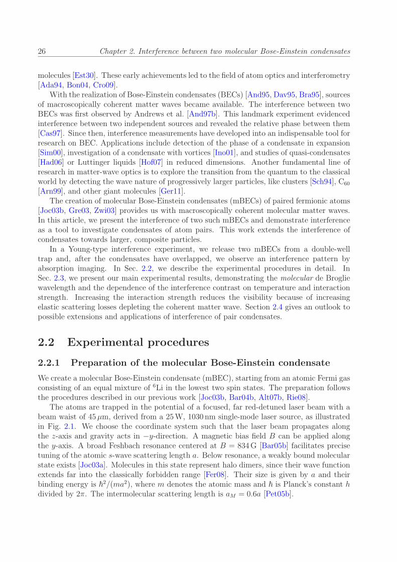
26 Chapter 2. Interference between two molecular Bose-Einstein condensates
molecules [Est30]. These early achievements led to the field of atom optics and interferometry[Ada94, Bon04, Cro09].
With the realization of Bose-Einstein condensates (BECs) [And95, Dav95, Bra95], sourcesof macroscopically coherent matter waves became available. The interference between twoBECs was first observed by Andrews et al. [And97b]. This landmark experiment evidencedinterference between two independent sources and revealed the relative phase between them[Cas97]. Since then, interference measurements have developed into an indispensable tool forresearch on BEC. Applications include detection of the phase of a condensate in expansion[Sim00], investigation of a condensate with vortices [Ino01], and studies of quasi-condensates[Had06] or Luttinger liquids [Hof07] in reduced dimensions. Another fundamental line ofresearch in matter-wave optics is to explore the transition from the quantum to the classicalworld by detecting the wave nature of progressively larger particles, like clusters [Sch94], C60
[Arn99], and other giant molecules [Ger11].The creation of molecular Bose-Einstein condensates (mBECs) of paired fermionic atoms
[Joc03b, Gre03, Zwi03] provides us with macroscopically coherent molecular matter waves.In this article, we present the interference of two such mBECs and demonstrate interferenceas a tool to investigate condensates of atom pairs. This work extends the interference ofcondensates towards larger, composite particles.
In a Young-type interference experiment, we release two mBECs from a double-welltrap and, after the condensates have overlapped, we observe an interference pattern byabsorption imaging. In Sec. 2.2, we describe the experimental procedures in detail. InSec. 2.3, we present our main experimental results, demonstrating the molecular de Brogliewavelength and the dependence of the interference contrast on temperature and interactionstrength. Increasing the interaction strength reduces the visibility because of increasingelastic scattering losses depleting the coherent matter wave. Section 2.4 gives an outlook topossible extensions and applications of interference of pair condensates.
2.2 Experimental procedures
2.2.1 Preparation of the molecular Bose-Einstein condensate
We create a molecular Bose-Einstein condensate (mBEC), starting from an atomic Fermi gasconsisting of an equal mixture of 6Li in the lowest two spin states. The preparation followsthe procedures described in our previous work [Joc03b, Bar04b, Alt07b, Rie08].
The atoms are trapped in the potential of a focused, far red-detuned laser beam with abeam waist of 45µm, derived from a 25W, 1030 nm single-mode laser source, as illustratedin Fig. 2.1. We choose the coordinate system such that the laser beam propagates alongthe z-axis and gravity acts in −y-direction. A magnetic bias field B can be applied alongthe y-axis. A broad Feshbach resonance centered at B = 834G [Bar05b] facilitates precisetuning of the atomic s-wave scattering length a. Below resonance, a weakly bound molecularstate exists [Joc03a]. Molecules in this state represent halo dimers, since their wave functionextends far into the classically forbidden range [Fer08]. Their size is given by a and theirbinding energy is ~2/(ma2), where m denotes the atomic mass and ~ is Planck’s constant hdivided by 2π. The intermolecular scattering length is aM = 0.6a [Pet05b].
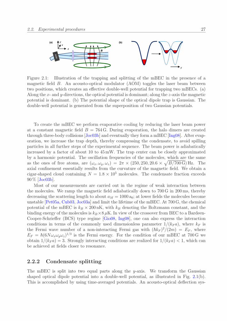
2.2. Experimental procedures 27
(b)(a) y
y
xz B
Figure 2.1: Illustration of the trapping and splitting of the mBEC in the presence of amagnetic field B. An acousto-optical modulator (AOM) toggles the laser beam betweentwo positions, which creates an effective double-well potential for trapping two mBECs. (a)Along the x- and y-directions, the optical potential is dominant; along the z-axis the magneticpotential is dominant. (b) The potential shape of the optical dipole trap is Gaussian. Thedouble-well potential is generated from the superposition of two Gaussian potentials.
To create the mBEC we perform evaporative cooling by reducing the laser beam powerat a constant magnetic field B = 764G. During evaporation, the halo dimers are createdthrough three-body collisions [Joc03b] and eventually they form a mBEC [Ing08]. After evap-oration, we increase the trap depth, thereby compressing the condensate, to avoid spillingparticles in all further steps of the experimental sequence. The beam power is adiabaticallyincreased by a factor of about 10 to 45mW. The trap center can be closely approximatedby a harmonic potential. The oscillation frequencies of the molecules, which are the sameas the ones of free atoms, are (ωx, ωy, ωz) = 2π × (250, 250, 20.6 ×
√
B/700G)Hz. Theaxial confinement essentially results from the curvature of the magnetic field. We obtain acigar-shaped cloud containing N = 1.8 × 10⁵ molecules. The condensate fraction exceeds90% [Joc03b].
Most of our measurements are carried out in the regime of weak interaction betweenthe molecules. We ramp the magnetic field adiabatically down to 700G in 200ms, therebydecreasing the scattering length to about aM = 1000 a0; at lower fields the molecules becomeunstable [Pet05a, Cub03, Joc03a] and limit the lifetime of the mBEC. At 700G, the chemicalpotential of the mBEC is kB × 200 nK, with kB denoting the Boltzmann constant, and thebinding energy of the molecules is kB×8µK. In view of the crossover from BEC to a Bardeen-Cooper-Schrieffer (BCS) type regime [Gio08, Ing08], one can also express the interactionconditions in terms of the commonly used dimensionless parameter 1/(kFa), where kF isthe Fermi wave number of a non-interacting Fermi gas with (~kF )
2/(2m) = EF , whereEF = ~(6Nωxωyωz)
1/3 is the Fermi energy. For the condition of our mBEC at 700G weobtain 1/(kFa) = 3. Strongly interacting conditions are realized for 1/(kFa) < 1, which canbe achieved at fields closer to resonance.
2.2.2 Condensate splitting
The mBEC is split into two equal parts along the y-axis. We transform the Gaussianshaped optical dipole potential into a double-well potential, as illustrated in Fig. 2.1(b).This is accomplished by using time-averaged potentials. An acousto-optical deflection sys-
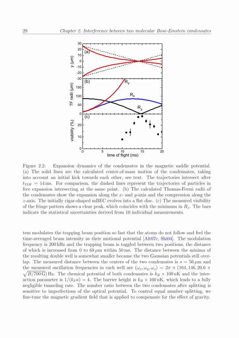
28 Chapter 2. Interference between two molecular Bose-Einstein condensates
Figure 2.2: Expansion dynamics of the condensates in the magnetic saddle potential.(a) The solid lines are the calculated center-of-mass motion of the condensates, takinginto account an initial kick towards each other, see text. The trajectories intersect aftertTOF = 14ms. For comparison, the dashed lines represent the trajectories of particles infree expansion intersecting at the same point. (b) The calculated Thomas-Fermi radii ofthe condensates show the expansion along the x- and y-axis and the compression along thez-axis. The initially cigar-shaped mBEC evolves into a flat disc. (c) The measured visibilityof the fringe pattern shows a clear peak, which coincides with the minimum in Rz. The barsindicate the statistical uncertainties derived from 10 individual measurements.
tem modulates the trapping beam position so fast that the atoms do not follow and feel thetime-averaged beam intensity as their motional potential [Alt07c, Shi04]. The modulationfrequency is 200 kHz and the trapping beam is toggled between two positions, the distanceof which is increased from 0 to 68µm within 50ms. The distance between the minima ofthe resulting double well is somewhat smaller because the two Gaussian potentials still over-lap. The measured distance between the centers of the two condensates is s = 56µm andthe measured oscillation frequencies in each well are (ωx, ωy, ωz) = 2π × (164, 146, 20.6 ×√
B/700G)Hz. The chemical potential of both condensates is kB × 100 nK and the inter-action parameter is 1/(kFa) = 4. The barrier height is kB × 160 nK, which leads to a fullynegligible tunneling rate. The number ratio between the two condensates after splitting issensitive to imperfections of the optical potential. To control equal number splitting, wefine-tune the magnetic gradient field that is applied to compensate for the effect of gravity.

2.2. Experimental procedures 29
2.2.3 Expansion in the magnetic field
The specific expansion dynamics of the released mBECs in our setup is the key to makinginterference clearly observable, and the understanding of the expansion is essential for theinterpretation of our results. We identify two effects, which result from the curvature of themagnetic field, that are favorable for the observation of interference.
The coils generating the magnetic offset field in our set-up are not in Helmholtz configu-ration, which leads to second-order terms in B(x, y, z). The resulting magnetic potential isa saddle potential, where the molecules are trapped along the x- and z-directions, but theyare anti-trapped along the y-axis, the symmetry axis of the field. The oscillation frequenciesare (ωx, ωy, ωz) = 2π × (20.5, i × 29, 20.5) ×
√
B/700GHz, where the imaginary frequencydenotes the anti-trap along the y-axis.
We model the expansion by adopting the scaling approach as applied in Refs. [Men02,Alt07c]. Figure 2.2(b) shows the predicted evolution of the Thomas-Fermi (TF) radii Rx, Ry
and Rz, which we also verify experimentally. At the beginning, the expansion is driven bythe pressure gradient in the cloud, which leads to a fast acceleration in the radial direction.This expansion is then further accelerated along y and decelerated along x because of themagnetic saddle potential. Along the z-axis, the long axis of the trapped cloud, the trapremains basically unchanged when the cloud is released from the optical potential. As themean field pressure of the expanding cloud decreases, the magnetic confinement leads to aspatial compression of the cloud. We find that after tTOF ≈ 14ms the parameter Rz has aminimum because of this compression effect.
For high interference contrast, large overlap of the two clouds at the time of detectionis essential. To achieve this, the condensates are kicked towards each other by switching onthe original single-well trap, typically for 0.1ms right after release from the double well. Thesolid lines in Fig. 2.2(a) show the calculated center-of-mass motion of the clouds after theinitial kick to assure large overlap at tTOF ≈ 14ms.
The interference pattern is determined by the relative velocity between the two conden-sates. The relative velocity vrel at y = 0 and tTOF = 14ms can be directly deduced fromthe slopes of the solid lines in Fig. 2.2(a). This velocity is substantially smaller than itwould be in free expansion without magnetic potential, where particles meeting at y = 0and tTOF = 14ms would follow the dashed trajectories in Fig. 2.2(a). This deceleration ofvrel can be readily visualized by the condensates climbing up the potential hill resulting fromthe anti-trap in y-direction. This anti-trap also accelerates the expansion in y-direction, seeRy in Fig. 2.2(b). Remarkably, since the velocity field in each of the clouds stays linear, vrelis independent of the position. More rigorously, we calculate vrel using the scaling approachand taking into account the center-of-mass motion of the clouds.
Thus expansion dynamics brings about two favorable effects: First, the spatial compres-sion along the z-axis facilitates clear detection of interference fringes by absorption imaging.Second, the decreased relative velocity leads to an increased fringe period. This means thatthe anti-trap acts as a magnifying glass for the interference fringes.

30 Chapter 2. Interference between two molecular Bose-Einstein condensates
0 50 1000
0.5
1
y (µm)
D/D
0 0.05 0.10
50
ky (2 /µm) F
(D) (
arb.
u.)
(b) (c)
max
(a)
x
y
Figure 2.3: Interference image and analysis. (a) The column density along the z-axis aftertTOF = 14ms shows the interference pattern. The field-of-view is 660µm×170µm. Theinner box indicates the region used for analysis. (b) The column density integrated alongx gives the density distribution D along y (dots). The solid curve is the result of the fit inFourier space, see text. (c) The density distribution is Fourier transformed (dots) and fitted(bars).
2.2.4 Detection and analysis of interference fringes
We detect the clouds by absorption imaging. Figure 2.3(a) shows a typical image of in-terference after 14ms time of flight. The imaging beam propagates along the z-axis. It isoverlapped with the trapping beam using dichroic mirrors. The imaging light pulse is on for10µs and its intensity is about the saturation intensity of 6Li atoms. We state-selectivelyimage the atoms in the second-to-lowest Zeeman state. Already the first photon scatteringevent is likely to dissociate the weakly bound molecule [Bar04b], followed by about 10 morephotons scattered by the free atom.
From the absorption images, we determine the visibility and fringe period of the interfer-ence pattern. The column density is integrated along the x-direction over the region depictedin Fig. 2.3(a) 1 resulting in a one-dimensional density distribution D, shown in Fig. 2.3(b).The density distribution contains various kinds of noise (e.g. photon or atom shot noise,or camera readout noise), which may be misinterpreted as interference signal. Thereforewe analyze the density distribution in Fourier space by considering the Fourier transformeddensity distribution F(D), see Fig. 2.3(c). Here all those types of noise are approximatelywhite and show up as a constant offset, whereas, the signal of interference is monochromaticand shows up as a peak. This gives the possibility to subtract the average contributionof noise from the signal. We determine the visibility and fringe period by the custom fit
1The size of the region was chosen to produce the optimal signal to noise.
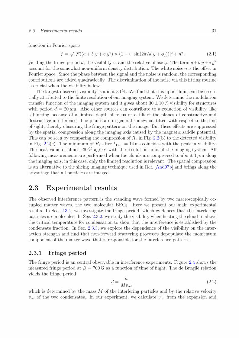
2.3. Experimental results 31
function in Fourier space
f =√
|F((a+ b y + c y2)× (1 + v sin(2π/d y + φ)))|2 + n2, (2.1)
yielding the fringe period d, the visibility v, and the relative phase φ. The term a+b y+c y2
account for the somewhat non-uniform density distribution. The white noise n is the offset inFourier space. Since the phase between the signal and the noise is random, the correspondingcontributions are added quadratically. The discrimination of the noise via this fitting routineis crucial when the visibility is low.
The largest observed visibility is about 30%. We find that this upper limit can be essen-tially attributed to the finite resolution of our imaging system. We determine the modulationtransfer function of the imaging system and it gives about 30± 10% visibility for structureswith period d = 20µm. Also other sources can contribute to a reduction of visibility, likea blurring because of a limited depth of focus or a tilt of the planes of constructive anddestructive interference. The planes are in general somewhat tilted with respect to the lineof sight, thereby obscuring the fringe pattern on the image. But these effects are suppressedby the spatial compression along the imaging axis caused by the magnetic saddle potential.This can be seen by comparing the compression of Rz in Fig. 2.2(b) to the detected visibilityin Fig. 2.2(c). The minimum of Rz after tTOF = 14ms coincides with the peak in visibility.The peak value of almost 30% agrees with the resolution limit of the imaging system. Allfollowing measurements are performed when the clouds are compressed to about 1µm alongthe imaging axis; in this case, only the limited resolution is relevant. The spatial compressionis an alternative to the slicing imaging technique used in Ref. [And97b] and brings along theadvantage that all particles are imaged.
2.3 Experimental results
The observed interference pattern is the standing wave formed by two macroscopically oc-cupied matter waves, the two molecular BECs. Here we present our main experimentalresults. In Sec. 2.3.1, we investigate the fringe period, which evidences that the interferingparticles are molecules. In Sec. 2.3.2, we study the visibility when heating the cloud to abovethe critical temperature for condensation to show that the interference is established by thecondensate fraction. In Sec. 2.3.3, we explore the dependence of the visibility on the inter-action strength and find that non-forward scattering processes depopulate the momentumcomponent of the matter wave that is responsible for the interference pattern.
2.3.1 Fringe period
The fringe period is an central observable in interference experiments. Figure 2.4 shows themeasured fringe period at B = 700G as a function of time of flight. The de Broglie relationyields the fringe period
d =h
Mvrel, (2.2)
which is determined by the mass M of the interfering particles and by the relative velocityvrel of the two condensates. In our experiment, we calculate vrel from the expansion and

32 Chapter 2. Interference between two molecular Bose-Einstein condensates
10 12 14 16 180
10
20
30
40
50
60molecules
fring
e pe
riod
(µm
)
time of flight (ms)
atoms
Figure 2.4: Fringe period as a function of time of flight. The symbols are the measuredperiods with bars, mostly smaller than the symbol size, indicating the statistical uncertaintiesresulting from 10 individual measurements at a given time of flight. The solid line is thecalculated period for molecules and the dashed line for atoms. For free expansion withoutthe magnetic saddle potential, the fringe period of molecules would be much smaller (dottedline).
center-of-mass motion of the condensates in the magnetic field curvature, as discussed inSec. 2.2.3. The result is in contrast to the simple relation vrel = s/tTOF that holds for the freeexpansion usually considered in experiments of this type. The solid line in Fig. 2.4 displaysthe calculated fringe period d for molecules, where we set M = 2m. All input parametersfor this calculation are determined independently. Their combined uncertainties result intypical uncertainty of 3% for the fringe period, with the main contribution stemming fromthe uncertainty in the cloud separation. The data are in remarkable agreement with thecalculation. For comparison, we also plot the fringe period for interfering atoms (M = m),which is clearly incompatible with the data.
The dotted line in Fig. 2.4 displays the fringe period that would result for freely expandingmBECs without the magnetic saddle potential. Comparing this curve to the much largerfringe period that we observe, highlights the effect of the magnetic field curvature to magnifythe fringe period, as discussed in Sec. 2.2.3. The same magnification effect was reported inRef. [Zaw10].
Note that the fringe period can be increased by interaction-induced slowing down ofthe two overlapping condensates [Sim00]. The mean-field of one condensate represents apotential hill for the other condensate, which slows down when climbing this hill. Under ourexperimental conditions at 700G, the effect is found to be negligible. For stronger interaction,we see indications of this effect in agreement with a corresponding model calculations.
2.3.2 Dependence of interference visibility on condensate fraction
To demonstrate that the interference results only from the condensed molecules and notfrom the thermal fraction, we perform a controlled heating experiment and show the loss
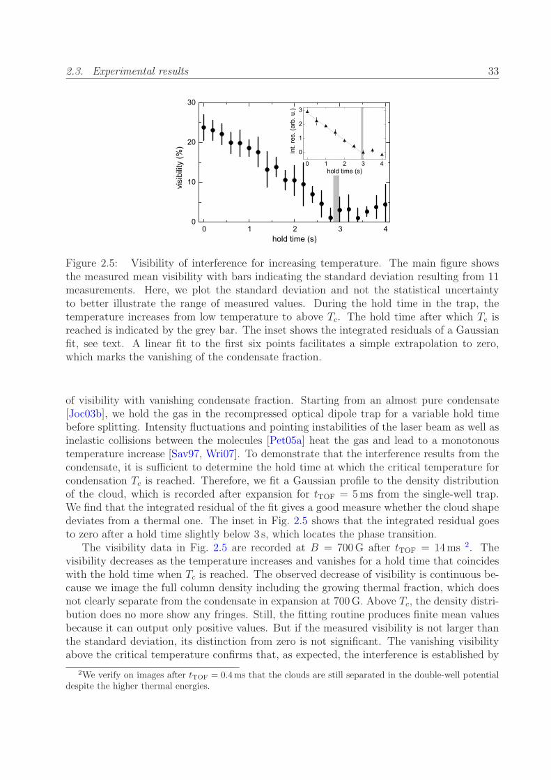
2.3. Experimental results 33
0 1 2 3 40
10
20
30
visi
bilit
y (%
)
hold time (s)
0 1 2 3 4
0
1
2
3
hold time (s)
int.
res.
(arb
. u.)
Figure 2.5: Visibility of interference for increasing temperature. The main figure showsthe measured mean visibility with bars indicating the standard deviation resulting from 11measurements. Here, we plot the standard deviation and not the statistical uncertaintyto better illustrate the range of measured values. During the hold time in the trap, thetemperature increases from low temperature to above Tc. The hold time after which Tc isreached is indicated by the grey bar. The inset shows the integrated residuals of a Gaussianfit, see text. A linear fit to the first six points facilitates a simple extrapolation to zero,which marks the vanishing of the condensate fraction.
of visibility with vanishing condensate fraction. Starting from an almost pure condensate[Joc03b], we hold the gas in the recompressed optical dipole trap for a variable hold timebefore splitting. Intensity fluctuations and pointing instabilities of the laser beam as well asinelastic collisions between the molecules [Pet05a] heat the gas and lead to a monotonoustemperature increase [Sav97, Wri07]. To demonstrate that the interference results from thecondensate, it is sufficient to determine the hold time at which the critical temperature forcondensation Tc is reached. Therefore, we fit a Gaussian profile to the density distributionof the cloud, which is recorded after expansion for tTOF = 5ms from the single-well trap.We find that the integrated residual of the fit gives a good measure whether the cloud shapedeviates from a thermal one. The inset in Fig. 2.5 shows that the integrated residual goesto zero after a hold time slightly below 3 s, which locates the phase transition.
The visibility data in Fig. 2.5 are recorded at B = 700G after tTOF = 14ms 2. Thevisibility decreases as the temperature increases and vanishes for a hold time that coincideswith the hold time when Tc is reached. The observed decrease of visibility is continuous be-cause we image the full column density including the growing thermal fraction, which doesnot clearly separate from the condensate in expansion at 700G. Above Tc, the density distri-bution does no more show any fringes. Still, the fitting routine produces finite mean valuesbecause it can output only positive values. But if the measured visibility is not larger thanthe standard deviation, its distinction from zero is not significant. The vanishing visibilityabove the critical temperature confirms that, as expected, the interference is established by
2We verify on images after tTOF = 0.4ms that the clouds are still separated in the double-well potentialdespite the higher thermal energies.

34 Chapter 2. Interference between two molecular Bose-Einstein condensates
650 700 750 800 8340
10
20
30
visi
bilit
y (%
)
magnetic field (G)
0
2
4
6
a M (1
000
a 0)
Figure 2.6: Visibility of interference from weak to strong interaction. The upper panelshows how the molecular scattering length aM increases towards the Feshbach resonance at834G, marked by the dashed line. The onset of the strongly interacting regime is markedby the dotted line. In the lower panel, the dots represent the mean visibility with barsindicating the standard deviation resulting from 20 individual measurements. The solid lineis the predicted visibility from the simple calculation modeling the non-forward scatteringevents.
the condensate fraction.
Further intriguing evidence that the interference is caused by the condensate is the ob-servation of interference between independent ultracold clouds. An independent productionrules out that the interference can be caused by self interference of particles [Mil05]. Toinvestigate interference between independent clouds, we split them already at a temperaturefar above the critical temperature to a large distance of 180µm and then create two mBECsindependently. Shortly before release, we reduce the distance to obtain the identical geom-etry as in all the other measurements and proceed as usual. We observe the same kind ofinterference pattern with a visibility of about 15%. The lower visibility can be explained bya less efficient evaporation and less control over the equal number preparation in the doublewell.
2.3.3 Dependence of interference visibility on interaction strength
In a further set of measurements, we investigate how the fringe visibility depends on the in-teraction strength. Therefore we perform the interference experiment for different magneticfield values, thereby changing the molecular scattering length aM according to the upper

2.3. Experimental results 35
panel of Fig. 2.6 3. The observed visibility as a function of the magnetic field is shown inthe lower panel in Fig. 2.6. The highest visibility is found at about 700G. For lower fields,the visibility is decreased, which we attribute to inelastic decay. The inelastic collisions ofmolecules lead to heating of the gas and loss of particles. The heating reduces the conden-sate fraction, which decreases the visibility as observed in the previous section. The lossalso reduces the signal on the images. This leads to a higher statistical uncertainty in thedetermination of the visibility, showing up in the larger standard deviations below 700G.
Towards larger interaction strength, our data show a pronounced decrease of visibility,and the visibility vanishes at about 780G. This coincides with the onset of strong interactionin the trap, where 1/kFa ≈ 1. We find that the main effect causing the decrease is elasticnon-forward scattering. It is known from experimental and theoretical work on collidingcondensates [Chi00, Ban00] that elastic non-forward scattering of particles removes themfrom the condensate wave function. In contrast to the forward scattering accounted for withinthe usual mean-field approach, this non-forward scattering transfers particles into momentumstates of random direction, which therefore do no more contribute to the observed interferencepattern. Non-forward scattering is a particle-like excitation, which requires vrel to exceedthe speed of sound vs. The process is suppressed for smaller vrel [Chi00, Ban01]. To estimatethe decrease of visibility through this process, we perform a simple model calculation. Thevelocity dependence of non-forward scattering is included by the following approximation:no suppression for vrel ≥ vs and full suppression otherwise. We calculate the mean numberof non-forward scattering events Ne for a representative molecule with molecules of the othercondensate until the moment of detection. This representative molecule travels along thecenter-of-mass path of the condensate; see Fig. 2.2(a). We take the bosonically enhanced,unitarity limited scattering cross section σ = 8πa2M/(1+(kaM)2), with k = mvrel/~. FromNe,we derive the probability for a molecule to still be part of the condensate. This probability ise−Ne and directly corresponds to the expected visibility, which we fit to the data, excludingthe three data points below 700G. We obtain the solid line in Fig. 2.6. The only fit parameteris a normalization factor, which allows us to account for the reduced detected visibilitybecause of the limited imaging resolution. The fit yields a factor of 0.32, which is consistentwith the imaging resolution discussed in Sec. 2.2.4. We find that our simple model for non-forward scattering can very well explain the decrease of visibility towards high interactionstrength.
There are also other effects that decrease the visibility for increasing interaction strength,but they turn out to be minor for our experimental conditions: Strong interaction lead toa depletion of the condensate [Dal99]. Only the condensate contributes to the interferencepattern and not the depleted fraction.The depleted fraction amounts to about 10% at 780G.As we expect the reduction of visibility to be proportional to the depletion, the reductionis negligible (at 780G from 2.6% to 2.3%). Another effect reducing the visibility is thecollisional dissociation of molecules during overlap. However, this effect can only occurabove 800G, where the collision energy exceeds the binding energy.
To directly demonstrate the effect of non-forward scattering, we study the collision of twocondensates when their relative velocity vrel is much faster than the their expansion velocity.
3We verify on images after tTOF = 0.4ms that the clouds are still separated in the double-well potentialdespite the higher chemical potential at higher interaction strength.
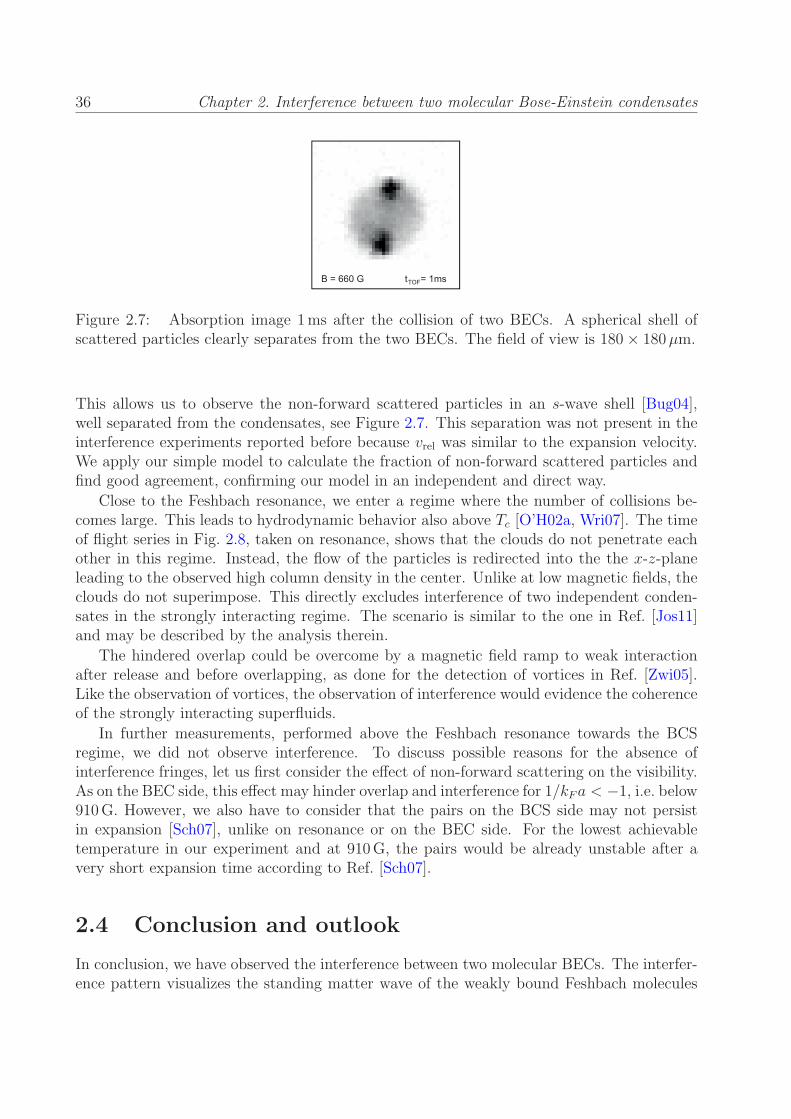
36 Chapter 2. Interference between two molecular Bose-Einstein condensates
B = 660 G t = 1msTOF
Figure 2.7: Absorption image 1ms after the collision of two BECs. A spherical shell ofscattered particles clearly separates from the two BECs. The field of view is 180× 180µm.
This allows us to observe the non-forward scattered particles in an s-wave shell [Bug04],well separated from the condensates, see Figure 2.7. This separation was not present in theinterference experiments reported before because vrel was similar to the expansion velocity.We apply our simple model to calculate the fraction of non-forward scattered particles andfind good agreement, confirming our model in an independent and direct way.
Close to the Feshbach resonance, we enter a regime where the number of collisions be-comes large. This leads to hydrodynamic behavior also above Tc [O’H02a, Wri07]. The timeof flight series in Fig. 2.8, taken on resonance, shows that the clouds do not penetrate eachother in this regime. Instead, the flow of the particles is redirected into the the x-z-planeleading to the observed high column density in the center. Unlike at low magnetic fields, theclouds do not superimpose. This directly excludes interference of two independent conden-sates in the strongly interacting regime. The scenario is similar to the one in Ref. [Jos11]and may be described by the analysis therein.
The hindered overlap could be overcome by a magnetic field ramp to weak interactionafter release and before overlapping, as done for the detection of vortices in Ref. [Zwi05].Like the observation of vortices, the observation of interference would evidence the coherenceof the strongly interacting superfluids.
In further measurements, performed above the Feshbach resonance towards the BCSregime, we did not observe interference. To discuss possible reasons for the absence ofinterference fringes, let us first consider the effect of non-forward scattering on the visibility.As on the BEC side, this effect may hinder overlap and interference for 1/kFa < −1, i.e. below910G. However, we also have to consider that the pairs on the BCS side may not persistin expansion [Sch07], unlike on resonance or on the BEC side. For the lowest achievabletemperature in our experiment and at 910G, the pairs would be already unstable after avery short expansion time according to Ref. [Sch07].
2.4 Conclusion and outlook
In conclusion, we have observed the interference between two molecular BECs. The interfer-ence pattern visualizes the standing matter wave of the weakly bound Feshbach molecules

2.4. Conclusion and outlook 37
B = 834 G t = 0.5 msTOF 1.5 ms 3.5 ms2.5 ms
y
x
Figure 2.8: The hindered overlap on resonance. The series shows the first few millisec-onds of expansion. The two clouds do not penetrate each other, but splash according tohydrodynamics. The field of view is 180× 180µm.
and shows coherence over the spatial extension of the cloud. The contrast of interferencevanishes above the critical temperature of condensation, demonstrating that the interferenceis established by the condensed molecules only. We find that non-forward elastic scatteringprocesses can lead to a depletion of the condensate wave function while the clouds overlap.This effect increases towards higher interaction strength and prevents us from observing in-terference in the strongly interacting regime. On resonance we observe that the two cloudsdo not overlap but rather collide and deform as a result of deep hydrodynamic behavior.
Interference between condensates of paired fermionic atoms can serve as a powerful toolto investigate many exciting aspects of those systems. A future application will be given, forexample, if p-wave condensates become available. Here, interference is predicted to revealthe vector nature of the order parameter [Zha07]. A conceptually interesting regime willbe entered when the size of the pairs becomes comparable to the fringe period. Then thedetected distribution of atoms may not reveal the interference pattern of the pair distribution.Besides investigating condensates of paired fermions themselves, the system could be usedto study the fundamental processes of interference. The wide tunability of the interactionstrength could be used to assist self-interference [Ced07] or to investigate to which extentinteraction build up the observable relative phase [Xio06].
Suppressing the effect of non-forward scattering during overlap could extend the rangeof applications of condensate interference. Such a suppression may be achieved by reducingthe interaction strength before overlap using fast magnetic field ramping techniques [Gre03,Zwi05]. This technique would allow for investigating the interference in the regime of stronginteraction or even on the BCS side of the resonance, where the interference of Cooper-typepairs is an intriguing question in itself.
Acknowledgments
We thank Christopher Gaul for stimulating discussions. We acknowledge support by theAustrian Science Fund (FWF) within SFB 15 (project part 21) and SFB 40 (project part 4).
38 Chapter 2. Interference between two molecular Bose-Einstein condensates
Chapter 3
Publication: Higher-nodal collective
modes in a resonantly interacting
Fermi gas†
accepted for publication in PRA (2013)
Edmundo R. Sanchez Guajardo, Meng Khoon Tey, Leonid A. Sidorenkov,and Rudolf Grimm
Institut fur Quantenoptik und Quanteninformation (IQOQI), Osterreichische Akademie der Wissenschaftenand Institut fur Experimentalphysik, Universitat Innsbruck, 6020 Innsbruck, Austria
We report on experimental investigations of longitudinal collective oscillationsin a highly elongated, harmonically trapped two-component Fermi gas with res-onantly tuned s-wave interactions (‘unitary Fermi gas’). We focus on higher-nodal axial modes, which in contrast to the elementary modes have receivedlittle attention so far. We show how these modes can be efficiently excited usinga resonant local excitation scheme and sensitively analyzed by a Fourier trans-formation of the detected time evolution of the axial density profile. We studythe temperature dependence of the mode frequencies across the superfluid phasetransition. The behavior is qualitatively different from the elementary modes,where the mode frequencies are independent of the temperature as long as thegas stays in the hydrodynamic regime. Our results are compared to theoreti-cal predictions based on Landau’s two-fluid theory and available experimentalknowledge of the equation of state. The comparison shows excellent agreementand thus both represents a sensitive test for the validity of the theoretical ap-proach and provides an independent test of the equation of state. The presentresults obtained on modes of first-sound character represent benchmarks for theobservation of second-sound propagation and corresponding oscillation modes.
†The author of the present thesis performed the measurements and data analysis, together with E.R.S.G.and M.K.T., under the supervision of R.G.
39
40 Chapter 3. Higher-nodal collective modes
3.1 Introduction
In ultracold quantum gases, measurements on collective oscillations are well established aspowerful tools to study the many-body properties of the system [Pit03, Pet02]. Experimentson collective modes reveal the dynamics in the different regimes of superfluid, collisionallyhydrodynamic, and collisionless behavior. The eigenfrequencies can be determined veryaccurately, which allows to extract valuable information on the equation of state (EOS),with great sensitivity to subtle interaction effects in the strongly interacting regime.
In ultracold Fermi gases [Ing08, Gio08, Blo08], collective modes have been widely appliedto study the crossover from Bose-Einstein condensation (BEC) to a Bardeen-Cooper-Shrieffer(BCS) type superfluid. A situation of particular interest is the two-component Fermi gaswith resonant interactions, with an s-wave scattering length tuned to infinity by meansof a Feshbach resonance [Chi10]. This special case, which lies right in the center of theBEC-BCS crossover, has attracted a great deal of interest, mainly attributed to its universalproperties. The resonantly interacting Fermi gas is characterized by strong interaction effectsin the EOS [Kin05b, Hor10, Nas10, Ku12] and reveals a unique universal thermodynamicbehavior [Ho04].
So far, experiments on collective modes in harmonically trapped Fermi gases have beenrestricted to a few elementary modes. The most simple modes, sloshing modes, do notprovide any information on the properties of the quantum gas, and their main applicationis thus to accurately determine the trap frequencies. Surface modes are insensitive to theEOS, but they allow to clearly distinguish between hydrodynamic and collisionless behav-ior [Alt07c, Wri07] and they have been used to detect the angular momentum in a rotatingFermi gas [Rie09, Rie11]. Elementary compression modes of axial [Bar04a, Nas09] and radial[Bar04a, Kin04a, Kin04b, Kin05a, Alt07b, Rie08] character have been very widely studiedin the field. Such modes do not only probe the particular collision regime, but they alsogive access to the compressibility of the gas. However, for a unitary Fermi gas, the eigenfre-quencies of the simple compression modes do not show any variation across the superfluidphase transition as the temperature is varied [Kin05a, Rie08]. This can be understood asa consequence of the fact that superfluid and collisional hydrodynamics both lead to thesame frequencies. A rigorous proof for this temperature-independence can be given in termsof an exact scaling solution of the hydrodynamic equations of motion [Hou13a]. The sit-uation is strikingly different for higher-nodal modes. Here the frequencies vary across thesuperfluid phase transition, when the dynamical regime changes from superfluid to collisionalhydrodynamics [Tey13, Hou13b]. Such higher-nodal modes therefore represent an interestingaddition to the experimental tool-box for probing strongly interacting Fermi gases.
We have recently carried out a series of experiments on higher-nodal axial modes in thegeometry of a highly elongated trapping potential. First results on the temperature depen-dence have already been presented in Ref. [Tey13], and the general theoretical framework isdescribed in Ref. [Hou13b]. In this Article, we briefly summarize the main theoretical pre-dictions (Sec. 3.2), we describe the experimental procedures in more detail (Sec. 3.3), andwe present the whole set of our experimental results obtained for two different higher-nodalmodes (Sec. 3.4). While we here restrict our attention to modes of first-sound character,we note that the results are important as benchmarks for the observation of second-sound
3.2. Theoretical predictions 41
propagation [Sid13] and in view of future experiments on second-sound modes (Sec. 3.5).
3.2 Theoretical predictions
Higher-nodal collective modes in Fermi gases have been theoretically studied based on Lan-dau’s two-fluid equations for an isotropic harmonic trapping geometry [He07, Tay09]. Forreal experiments, however, the situation of highly elongated harmonic traps is more rele-vant. In this geometry, the description can be reduced to a set of effectively 1D hydrody-namic equations, which only depend on the axial coordinate z. This simplification leads toa powerful approach to describe sound propagation and collective modes in experimentallyrealistic situation. The basic approach was introduced in Ref. [Ber10] for a cylindrical trapgeometry with tight radial confinement. Reference [Hou13b] presents a generalization to thesituation of additional weak axial confinement, which readily describes the commonly usedgeometry of a highly elongated trap containing a ‘cigar-shaped’ atomic sample. Here, wesummarize the main elements of this theoretical approach and the corresponding predictionsfor higher-nodal modes of first-sound character.
The two basic assumptions underlying the 1D hydrodynamic approach are thermal equi-librium in the radial direction and a flow field that is independent of the radial position.This corresponds to conditions of sufficient heat conductivity and sufficient shear viscosity,which are readily satisfied for resonantly interacting Fermi gases under common trappingconditions. Applying the local density approximation, one can describe the thermodynamicsand the flow properties of the trapped sample using effective 1D quantities, which are derivedby integrating over the transverse degrees of freedom, such that a thermodynamic quantityq yields a 1D counterpart q1 = 2π
∫
∞
0q r dr.
For a first-sound collective mode with frequency ω, the local flow speed can be expressedas v(z, t) = vz(z)e
−iωt, where the z-dependent amplitude vz(z) represents the spatial os-cillation of the flow velocity. The hydrodynamic equation that describes vz(z) takes theform [Hou13b]
m(ω2 − ω2z)vz −
7
5mω2
zz∂zvz +7
5
P1
n1
∂2zvz = 0 . (3.1)
Here, ωz represents the trap frequency along the axial direction, m is the atomic mass, P1 isthe ‘1D pressure’ (having units of force), and n1 is the linear number density. The equationis valid for small-amplitude oscillations, which can be treated as perturbations by linearizingLandau’s equations.
At zero temperature and in the classical limit of high temperature the hydrodynamicequation (4.1) admits analytic solutions of polynomial form vz = akz
k + ak−2zk−2 + ..., with
integer values of k. At T = 0, where P1(n1)/n1 = (2/7)[µ0− (1/2)mω2zz
2], with µ0 being thechemical potential at the center of the trap, the frequency of the k-th mode is given by
ω2 =1
5(k + 1)(k + 5)ω2
z . (3.2)
In the classical limit, where P1/n1 = kBT , one finds the different k-dependence
ω2 =1
5(7k + 5)ω2
z . (3.3)

42 Chapter 3. Higher-nodal collective modes
We point out that Eqs. (4.2) and (4.3) give the same values for k = 0 (center of massoscillation) and k = 1 (lowest axial breathing mode). In fact, one can prove that the frequen-cies of these two lowest modes are temperature independent for the resonantly interactinggas (unitary Fermi gas), corresponding to an exact scaling solution of the two-fluid hydro-dynamic equation [Hou13a]. On contrary, the frequencies of the k ≥ 2 modes vary withtemperature.
We now focus on the modes with k = 2 and k = 3, which are experimentally mostrelevant. Using a variational approach [Tay08], one can obtain their eigenfrequencies atfinite temperatures as
ω2k=2 =
129t2 − 25
5(9t2 − 5)ω2z , (3.4)
and
ω2k=3 =
440t3 − 252
5(25t3 − 21)ω2z . (3.5)
In these equations t2 = M0M4/M22 and t3 = M2M6/M
24 , where we have introduced the
dimensionless moments
Mℓ =
∫ βµ0
−∞
dx(βµ0 − x)(ℓ+1)/2fn(x). (3.6)
Here, the phase-space density fn(x) is a universal function [Ho04] defined by fn(x) = nλ3T ,where n is the 3D number density and λT = h/(2πmkBT )
1/2 is the thermal deBroglie wave-length. The dimensionless parameter x = βµ, with β = 1/kBT and µ being the chemicalpotential, is related uniquely to T/TF . The universal function fn(x) can be determined fromthe recent EOS measurements [Kin05b, Hor10, Nas10, Ku12]. In this work, we make use ofthe latest results from [Ku12].
One can also show that the velocity fields for the k = 2 and k = 3 modes take the form
vk=2z (z) ∝ 3mω2
zβ
2
M0(x0)
M2(x0)z2 − 1 , (3.7)
and
vk=3z (z) ∝ 5mω2
zβ
6
M2(x0)
M4(x0)z3 − z . (3.8)
Here, the parameter x0 = βµ0 is the value of x at the center of the trap. Finally, using theequation of continuity under the 1D formulation ∂tn1 + ∂z(n1vz) = 0, one can calculate theshape of the density oscillations for each mode.
3.3 Experimental procedures
3.3.1 Sample preparation
The starting point of our experiment is an ultracold, resonantly interacting Fermi gas in anelongated optical dipole trap. This gas is prepared by evaporating a balanced mixture offermionic 6Li atoms in their two lowest spin states at a magnetic field of 834G, very close to
3.3. Experimental procedures 43
the center of the well-known broad Feshbach resonance [Chi10] 1. The atomic cloud containstypically N/2 = 1.5×10⁵ atoms per spin state. For the lowest temperatures, the waist of thetrapping beam (wavelength 1075 nm) is 31 µm, the trap depth is about 2µK, and the axialand radial trap frequencies are ωz = 2π× 22.52(2)Hz and ωr = 2π× 473(2)Hz, respectively.For experiments at higher temperatures, the beam waist is increased to 38 µm, and deepertraps are used (up to 16µK depth) with trap frequencies of up to ωz = 2π× 23.31(3)Hz andωr = 2π × 1226(6)Hz. The corresponding Fermi temperatures TF = ~(3Nω2
rωz)1/3/kB vary
between about 0.8 and 1.5µK.To achieve the lowest possible temperatures, we perform deep evaporative cooling up to
the point where the trapping potential cuts slightly into the Fermi sea, indicated by theonset of spilling losses in the last stage of the evaporation. After that, the gas is adiabat-ically recompressed by increasing the trapping beam’s power to the extent where the trapdepth becomes at least twice more than the Fermi energy kBTF . This recompression stepis essential to ensure negligible anharmonicities in the radial confinement. The essentiallyperfect harmonic confinement along the axial direction is ensured by the magnetic trappingthat results from the curvature of the magnetic field used for Feshbach tuning [Joc03b].
We vary the temperature T of the gas by controlled heating, always starting from adeeply cooled cloud (T/TF ≈ 0.1). In the low-temperature range (T . 0.2TF ), we simplyintroduce a variable hold time of up to 4 s in which residual trap heating slowly increases thecloud’s temperature. For the higher-temperature range (0.2TF < T < 0.5TF ), we heat thesample using parametric heating, modulating the trap power at about 2ωr, and introducinga sufficient hold time to reach thermal equilibrium between the different degrees of freedom.We note that we use deeper traps for samples with higher T/TF , because plain evaporationputs a limit on the maximum attainable temperature of the gas.
3.3.2 Thermometry
We determine the temperature T of the gas by analyzing its density distribution in the trap,based on knowledge of the EOS. Under the local density approximation, one can readilyshow for a harmonic trap that the 1D density profile n1(z) is given by [Nas10, Ho10]
n1(z) =2π
mω2r
kBT
λ3Tfp(x0 −
1
2βmω2
zz2) . (3.9)
Here, the universal function fp(x) is related to the universal function fn(x) introduced inSec. 3.2 by fp(x) =
∫ x
−∞fn(y) dy, and is therefore also known from a given EOS. The
parameter x0 is the value of x at the center of the trap.In the ideal case where one is able to obtain an accurate in-situ measurement of n1(z)
by imaging the trapped cloud, it is straightforward to retrieve the parameters T and x0 byfitting n1(z) using Eq. (3.9). However, in reality we have to deal with imperfections of ourabsorption imaging scheme. To extract the temperature in an accurate way, we have adoptedthe methods described in detail in the Appendix.
1A very recent measurement [Zur13] pinpoints the pole of the resonance to 832.2 G. Our measure-ments were performed at 834 G, corresponding to the previous state of knowledge on the resonance posi-tion [Bar05b]. The difference, however, is less than 1% of the resonance width and therefore has negligibleeffect on the present measurements.
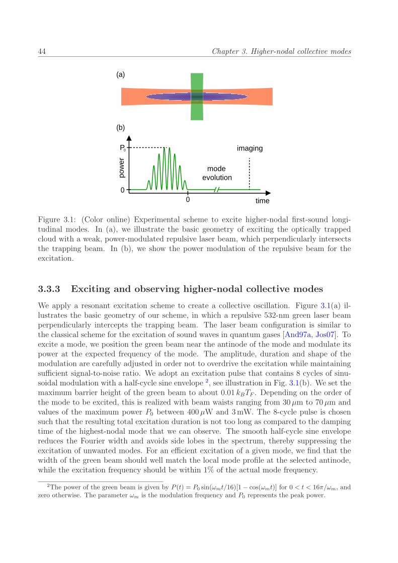
44 Chapter 3. Higher-nodal collective modes
imaging
time00
mode evolution
P0
(a)
(b)po
wer
Figure 3.1: (Color online) Experimental scheme to excite higher-nodal first-sound longi-tudinal modes. In (a), we illustrate the basic geometry of exciting the optically trappedcloud with a weak, power-modulated repulsive laser beam, which perpendicularly intersectsthe trapping beam. In (b), we show the power modulation of the repulsive beam for theexcitation.
3.3.3 Exciting and observing higher-nodal collective modes
We apply a resonant excitation scheme to create a collective oscillation. Figure 3.1(a) il-lustrates the basic geometry of our scheme, in which a repulsive 532-nm green laser beamperpendicularly intercepts the trapping beam. The laser beam configuration is similar tothe classical scheme for the excitation of sound waves in quantum gases [And97a, Jos07]. Toexcite a mode, we position the green beam near the antinode of the mode and modulate itspower at the expected frequency of the mode. The amplitude, duration and shape of themodulation are carefully adjusted in order not to overdrive the excitation while maintainingsufficient signal-to-noise ratio. We adopt an excitation pulse that contains 8 cycles of sinu-soidal modulation with a half-cycle sine envelope 2, see illustration in Fig. 3.1(b). We set themaximum barrier height of the green beam to about 0.01 kBTF . Depending on the order ofthe mode to be excited, this is realized with beam waists ranging from 30µm to 70µm andvalues of the maximum power P0 between 400µW and 3mW. The 8-cycle pulse is chosensuch that the resulting total excitation duration is not too long as compared to the dampingtime of the highest-nodal mode that we can observe. The smooth half-cycle sine envelopereduces the Fourier width and avoids side lobes in the spectrum, thereby suppressing theexcitation of unwanted modes. For an efficient excitation of a given mode, we find that thewidth of the green beam should well match the local mode profile at the selected antinode,while the excitation frequency should be within 1% of the actual mode frequency.
2The power of the green beam is given by P (t) = P0 sin(ωmt/16)[1− cos(ωmt)] for 0 < t < 16π/ωm, andzero otherwise. The parameter ωm is the modulation frequency and P0 represents the peak power.
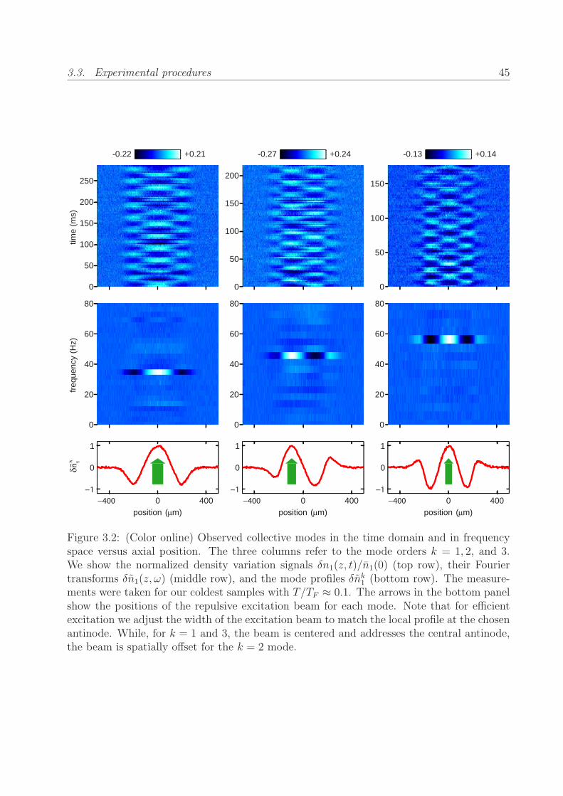
3.3. Experimental procedures 45
0
50
100
150
200
250
time
(ms)
0
20
40
60
80
freq
uenc
y (H
z)
0 400
0
1
position (mm)
0
50
100
150
200
0
20
40
60
80
0 400
0
1
position (mm)
0
50
100
150
0
20
40
60
80
0 400
0
1
position (mm)
+0.21-0.22 +0.24-0.27 +0.14-0.13
~
Figure 3.2: (Color online) Observed collective modes in the time domain and in frequencyspace versus axial position. The three columns refer to the mode orders k = 1, 2, and 3.We show the normalized density variation signals δn1(z, t)/n1(0) (top row), their Fouriertransforms δn1(z, ω) (middle row), and the mode profiles δnk
1 (bottom row). The measure-ments were taken for our coldest samples with T/TF ≈ 0.1. The arrows in the bottom panelshow the positions of the repulsive excitation beam for each mode. Note that for efficientexcitation we adjust the width of the excitation beam to match the local profile at the chosenantinode. While, for k = 1 and 3, the beam is centered and addresses the central antinode,the beam is spatially offset for the k = 2 mode.
46 Chapter 3. Higher-nodal collective modes
Once a collective mode is excited, we record the axial density profiles n1(z, t) of the gasfor a variable time delay t after the excitation pulse, where n1(z, t) is the number densityintegrated over the transverse degrees of freedom. These profiles are obtained with a probebeam that perpendicularly intercepts the trapping beam, and are taken 600µs after sud-denly releasing the atoms from the optical trap 3. To enhance the visibility, we subtract abackground profile n1(z) obtained from averaging the profiles over all measured delay times.This gives a differential density variation function δn1(z, t) = n1(z, t) − n1(z), which is fi-nally normalized to the maximum linear density n1(0) at the trap center. In the top panel ofFig. 3.2, we show examples of this signal for the k = 1, 2, and 3 modes for the coldest sam-ples with T/TF ≈ 0.1. One can see that the adjacent antinodes always oscillate in oppositedirections, similar to standing waves on a guitar string.
3.3.4 Analyzing the eigenmodes: Extracting mode profiles, fre-
quencies, and damping rates
The first step to analyze the observed time-dependent profiles δn1(z, t) is a Fourier transform,yielding a representation of our data in frequency space, δn1(z, ω)
4. For this purpose weemploy a fast Fourier transform (FFT) algorithm. Corresponding results are shown in themiddle panel of Fig. 3.2, as calculated for each time-dependent oscillation profile in the toppanel. The discrete nature in frequency space becomes evident, with very little noise in thebackground.
It is straightforward to extract the mode profiles δnk1(z) from the FFT results by setting
δnk1(z) = δn1(z, ωk), where ωk is the eigenfrequency of the kth mode. The corresponding
mode profiles for the k = 1, 2, and 3 modes are shown in the bottom panel of Fig. 3.2.Experimentally, we make use of the mode profiles and the frequencies obtained in this wayto optimize the beam waist and the modulation frequency in our excitation scheme. Weproceed iteratively, which eventually allows for an optimum excitation of a single mode.
To extract the mode frequencies more precisely than it is possible by simply analyzingthe peaks in the corresponding Fourier spectrum, we adopt the following algorithm. Weproject δn1(z, t) onto the mode profile δnk
1(z) to obtain a mode amplitude function A(t) =∫
∞
−∞δn1(z, t)δn
k1(z) dz. Then we fit a simple damped harmonic oscillation to A(t) to obtain
the frequency and the damping time of the mode. This projection procedure is analogousto the projection of a superposition wavefunction onto one of the orthogonal eigenstatesof a quantum system. It greatly enhances the signal-to-noise ratio and results in very lowstatistical uncertainties for the mode frequencies, with relative uncertainties as low as in therange of a few permille.
In Fig. 3.3, we show examples of A(t) for the k = 1, 2, and 3 modes obtained from
3The images are recorded after a short time of flight of 600 µs. The small radial expansion avoids verylarge optical densities and thus allows for a more accurate determination of the atom number. The effect onthe one-dimensional (doublyintegrated) axial density profile remains negligibly small, since the hydrodynamicexpansion of a cigar-shaped cloud proceeds mostly in the radial direction.
4FFT gives a complex spectrum, δn(z, ω) = Re[δn(z, ω)]+ i Im[δn(z, ω)]. By multiplying a suitable phasefactor to δn(z, ω), we can transfer all information pertaining to a particular mode into one quadrature,obtaining δn(z, ω).
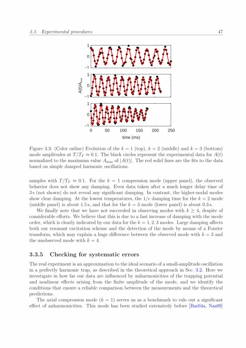
3.3. Experimental procedures 47
0
1
0
1
0 50 100 150 200 250
0
1
time (ms)
A(t
)/A
max
Figure 3.3: (Color online) Evolution of the k = 1 (top), k = 2 (middle) and k = 3 (bottom)mode amplitudes at T/TF ≈ 0.1. The black circles represent the experimental data for A(t)normalized to the maximum value Amax of |A(t)|. The red solid lines are the fits to the databased on simple damped harmonic oscillations.
samples with T/TF ≈ 0.1. For the k = 1 compression mode (upper panel), the observedbehavior does not show any damping. Even data taken after a much longer delay time of3 s (not shown) do not reveal any significant damping. In contrast, the higher-nodal modesshow clear damping. At the lowest temperatures, the 1/e damping time for the k = 2 mode(middle panel) is about 1.5 s, and that for the k = 3 mode (lower panel) is about 0.3 s.
We finally note that we have not succeeded in observing modes with k ≥ 4, despite ofconsiderable efforts. We believe that this is due to a fast increase of damping with the modeorder, which is clearly indicated by our data for the k = 1, 2, 3 modes. Large damping affectsboth our resonant excitation scheme and the detection of the mode by means of a Fouriertransform, which may explain a huge difference between the observed mode with k = 3 andthe unobserved mode with k = 4.
3.3.5 Checking for systematic errors
The real experiment is an approximation to the ideal scenario of a small-amplitude oscillationin a perfectly harmonic trap, as described in the theoretical approach in Sec. 3.2. Here weinvestigate in how far our data are influenced by anharmonicities of the trapping potentialand nonlinear effects arising from the finite amplitude of the mode, and we identify theconditions that ensure a reliable comparison between the measurements and the theoreticalpredictions.
The axial compression mode (k = 1) serves us as a benchmark to rule out a significanteffect of anharmonicities. This mode has been studied extensively before [Bar04a, Nas09]
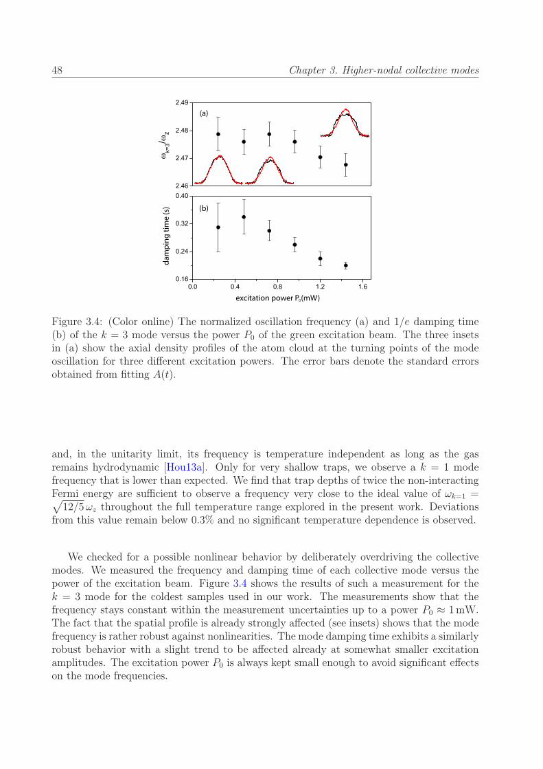
48 Chapter 3. Higher-nodal collective modes
z
excitation power P (mW)
(a)
da
mp
ing
tim
e (
s)
0
(b)
Figure 3.4: (Color online) The normalized oscillation frequency (a) and 1/e damping time(b) of the k = 3 mode versus the power P0 of the green excitation beam. The three insetsin (a) show the axial density profiles of the atom cloud at the turning points of the modeoscillation for three different excitation powers. The error bars denote the standard errorsobtained from fitting A(t).
and, in the unitarity limit, its frequency is temperature independent as long as the gasremains hydrodynamic [Hou13a]. Only for very shallow traps, we observe a k = 1 modefrequency that is lower than expected. We find that trap depths of twice the non-interactingFermi energy are sufficient to observe a frequency very close to the ideal value of ωk=1 =√
12/5ωz throughout the full temperature range explored in the present work. Deviationsfrom this value remain below 0.3% and no significant temperature dependence is observed.
We checked for a possible nonlinear behavior by deliberately overdriving the collectivemodes. We measured the frequency and damping time of each collective mode versus thepower of the excitation beam. Figure 3.4 shows the results of such a measurement for thek = 3 mode for the coldest samples used in our work. The measurements show that thefrequency stays constant within the measurement uncertainties up to a power P0 ≈ 1mW.The fact that the spatial profile is already strongly affected (see insets) shows that the modefrequency is rather robust against nonlinearities. The mode damping time exhibits a similarlyrobust behavior with a slight trend to be affected already at somewhat smaller excitationamplitudes. The excitation power P0 is always kept small enough to avoid significant effectson the mode frequencies.
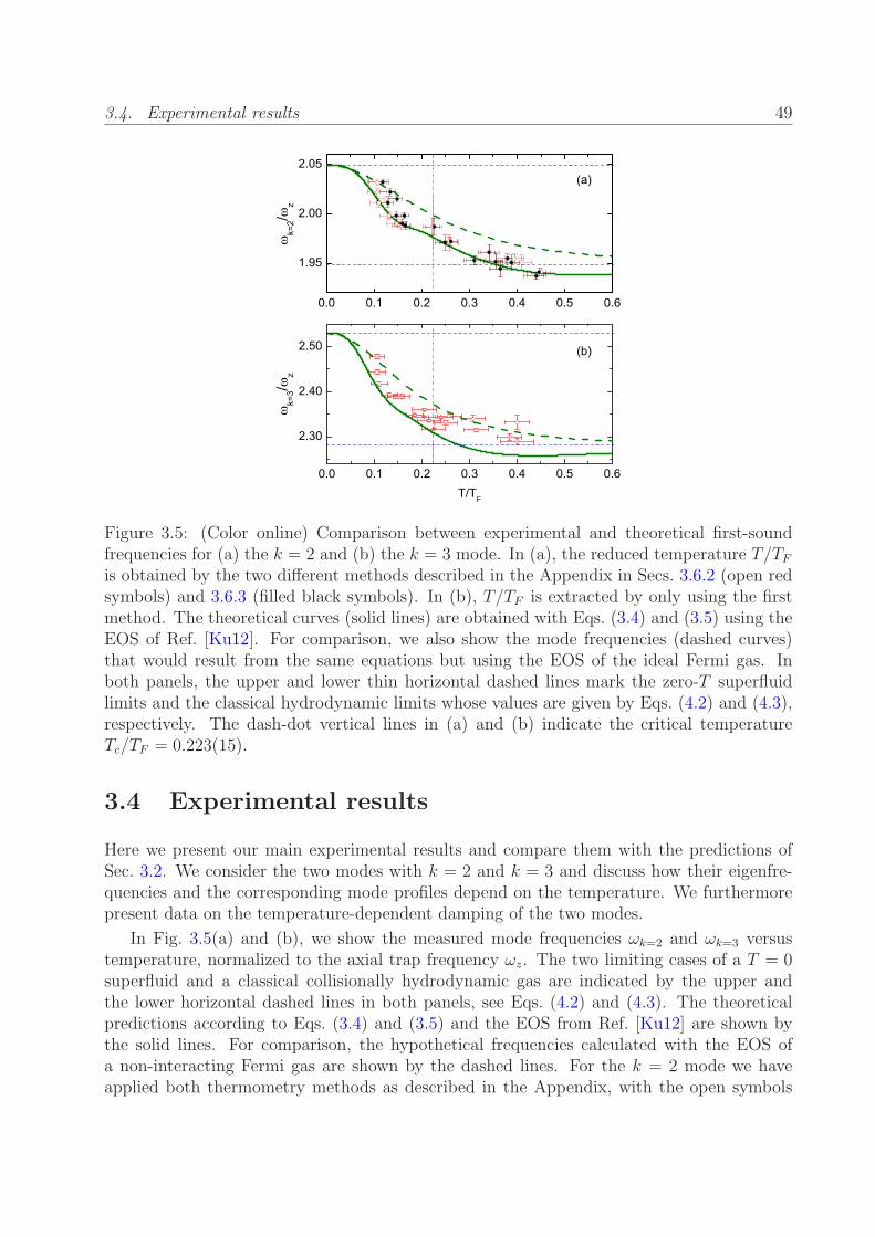
3.4. Experimental results 49
Figure 3.5: (Color online) Comparison between experimental and theoretical first-soundfrequencies for (a) the k = 2 and (b) the k = 3 mode. In (a), the reduced temperature T/TFis obtained by the two different methods described in the Appendix in Secs. 3.6.2 (open redsymbols) and 3.6.3 (filled black symbols). In (b), T/TF is extracted by only using the firstmethod. The theoretical curves (solid lines) are obtained with Eqs. (3.4) and (3.5) using theEOS of Ref. [Ku12]. For comparison, we also show the mode frequencies (dashed curves)that would result from the same equations but using the EOS of the ideal Fermi gas. Inboth panels, the upper and lower thin horizontal dashed lines mark the zero-T superfluidlimits and the classical hydrodynamic limits whose values are given by Eqs. (4.2) and (4.3),respectively. The dash-dot vertical lines in (a) and (b) indicate the critical temperatureTc/TF = 0.223(15).
3.4 Experimental results
Here we present our main experimental results and compare them with the predictions ofSec. 3.2. We consider the two modes with k = 2 and k = 3 and discuss how their eigenfre-quencies and the corresponding mode profiles depend on the temperature. We furthermorepresent data on the temperature-dependent damping of the two modes.
In Fig. 3.5(a) and (b), we show the measured mode frequencies ωk=2 and ωk=3 versustemperature, normalized to the axial trap frequency ωz. The two limiting cases of a T = 0superfluid and a classical collisionally hydrodynamic gas are indicated by the upper andthe lower horizontal dashed lines in both panels, see Eqs. (4.2) and (4.3). The theoreticalpredictions according to Eqs. (3.4) and (3.5) and the EOS from Ref. [Ku12] are shown bythe solid lines. For comparison, the hypothetical frequencies calculated with the EOS ofa non-interacting Fermi gas are shown by the dashed lines. For the k = 2 mode we haveapplied both thermometry methods as described in the Appendix, with the open symbols
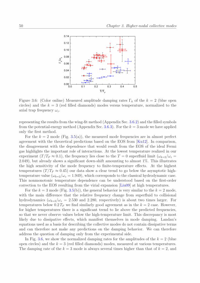
50 Chapter 3. Higher-nodal collective modes
Figure 3.6: (Color online) Measured amplitude damping rates Γk of the k = 2 (blue opencircles) and the k = 3 (red filled diamonds) modes versus temperature, normalized to theaxial trap frequency ωz.
representing the results from the wing-fit method (Appendix Sec. 3.6.2) and the filled symbolsfrom the potential-energy method (Appendix Sec. 3.6.3). For the k = 3 mode we have appliedonly the first method.
For the k = 2 mode (Fig. 3.5(a)), the measured mode frequencies are in almost perfectagreement with the theoretical predictions based on the EOS from [Ku12]. In comparison,the disagreement with the dependence that would result from the EOS of the ideal Fermigas highlights the important role of interactions. At the lowest temperature realized in ourexperiment (T/TF ≈ 0.1), the frequency lies close to the T = 0 superfluid limit (ωk=2/ωz =2.049), but already shows a significant down-shift amounting to almost 1%. This illustratesthe high sensitivity of the mode frequency to finite-temperature effects. At the highesttemperatures (T/TF ≈ 0.45) our data show a clear trend to go below the asymptotic high-temperature value (ωk=2/ωz = 1.949), which corresponds to the classical hydrodynamic case.This nonmonotonic temperature dependence can be understood based on the first-ordercorrection to the EOS resulting from the virial expansion [Liu09] at high temperatures.
For the k = 3 mode (Fig. 3.5(b)), the general behavior is very similar to the k = 2 mode,with the main difference that the relative frequency change from superfluid to collisionalhydrodynamics (ωk=2/ωz = 2.530 and 2.280, respectively) is about two times larger. Fortemperatures below 0.2TF we find similarly good agreement as in the k = 2 case. However,for higher temperatures there is a significant trend to lie above the predicted frequencies,so that we never observe values below the high-temperature limit. This discrepancy is mostlikely due to dissipative effects, which manifest themselves in mode damping. Landau’sequations used as a basis for describing the collective modes do not contain dissipative termsand can therefore not make any predictions on the damping behavior. We can thereforeaddress the question of damping only from the experimental side.
In Fig. 3.6, we show the normalized damping rates for the amplitudes of the k = 2 (blueopen circles) and the k = 3 (red filled diamonds) modes, measured at various temperatures.The damping rate of the k = 3 mode is always several times higher than that of k = 2, and

3.4. Experimental results 51
~~
Figure 3.7: (Color online) Comparison of experimental mode profiles (data points) andtheoretical predictions (solid lines) for two different temperatures. In (a), we show the cloudprofiles obtained with a 2-ms TOF. The solid lines show the density profiles obtained fromthe EOS [Ku12] with T/TF = 0.10 and 0.45. In (b), we show the experimental and theoreticalk = 2 mode profiles at the indicated temperatures. The comparison for the k = 3 mode ispresented in (c). The z scale is normalized to the Thomas-Fermi radius ZTF of the zero-Tinteracting gas, which is a factor of ξ1/4 ≈ 0.78 [Ku12] smaller than in the non-interactingcase.
it strongly increases as the cloud gets hotter. It is evident that the situation, where we haveobserved significant deviations in the mode frequencies (k = 3 and T/TF & 0.2), coincideswith the case of highest damping rates (exceeding 10 s−1). It is known that violation of the1D condition assumed in Sec. 3.2 would result in a damping of the collective oscillation.Therefore, a higher damping rate could naturally be accompanied with a larger deviationfrom the prediction using the 1D formulation of the Landau’s two-fluid model. This supportsour interpretation of the observed frequency deviation in terms of dissipative effects.
For an accurate determination of temperature-dependent frequency shifts in our experi-ment, the k = 2 mode turns out to be superior to the k = 3 mode. Our results indicate thatthe advantage of the latter mode to exhibit larger frequency changes is overcompensatedby the larger damping, which introduces larger statistical uncertainties (see error bars inFig. 3.5) and apparently also systematic errors. However, for larger trap aspect ratios thanapplied in our experiment, the situation may be different and higher modes may providefurther interesting information.
In Fig. 4.1(a) and (b), we finally show the observed spatial profiles of the k = 2 andk = 3 modes, in comparison to the corresponding theoretical predictions. For both modes
52 Chapter 3. Higher-nodal collective modes
we present data sets for the lowest temperature that we could realize (T/TF ≈ 0.1) and forthe highest temperature explored (T/TF ≈ 0.45). In the first case, the situation is deep in thesuperfluid regime, whereas the second case corresponds to the classical hydrodynamic case.For reference, Fig. 4.1(a) shows the corresponding spatial profiles of the unperturbed cloud,from which we obtained the temperature following the method of Sec. 3.6.3 in the Appendix.The agreement between the experimentally observed mode profiles and the theoretical pre-dictions is remarkable. Within the experimental uncertainties and with the mode amplitudebeing the only fit parameter, we find a perfect match. This again highlights the validityof the theoretical 1D framework and power of our experimental approach to higher-nodalcollective modes.
3.5 Conclusions and Outlook
We have presented an efficient tool-box to excite and detect higher-nodal axial collectivemodes in a resonantly interacting Fermi gas. Our results (see also [Tey13]) reveal the pro-nounced temperature dependence below and near the superfluid phase transition, which istheoretically predicted in the framework of a 1D two-fluid hydrodynamic model [Hou13b].The observed temperature dependence is a unique feature of higher-nodal modes and hasnot been observed in any other collective mode studied in Fermi gases so far. The excellentagreement of the experimentally observed mode frequencies with the theoretical predictionsprovides a stringent test for the validity of this 1D approach and provides an independentconfirmation of the recently measured EOS [Ku12] of the resonantly interacting Fermi gas.
We have also reported first studies on the mode damping behavior, which show a strongincrease of the measured damping rates with the order of the mode investigated. Dedicatedexperiments on damping could provide valuable information on the viscosity and the thermalconductivity of the strongly interacting Fermi gas, which may provide further insight intofundamental questions related to viscosity [Sch09, Cao11a, Cao11b]. A better understandingof damping would also be important to understand the limitations of the theoretical approach[Hou13b] applied to describe the modes.
Generalizations of our experiments to first-sound collective modes in the BEC-BCScrossover regime [Gio08, Blo08, Chi10]) and to spin-polarized Fermi gases [Zwi06b, Par06,Nas09] will be rather straightforward. A very exciting prospect is the extension to second-sound modes [Tay09, Hou13b], where the superfluid and the normal component oscillate inopposite phase. A recent experiment [Sid13] shows the propagation of second-sound pulsesalong the trap axis, in agreement with a theoretical description based on the same approachthat is used in the present work. This observation may, in principle, be interpreted in terms ofa superposition of several second-sound modes, but the selective excitation and observationof individual modes of this kind remains an experimental challenge for future experiments.
We would like to acknowledge the strong theoretical support from Yan-Hua Hou, LevPitaevskii, and Sandro Stringari. We thank Mark Ku and Martin Zwierlein for fruitfuldiscussions and Florian Schreck for discussion and experimental support. We acknowledgesupport from the Austrian Science Fund (FWF) within SFB FoQuS (project No. F4004-N16).
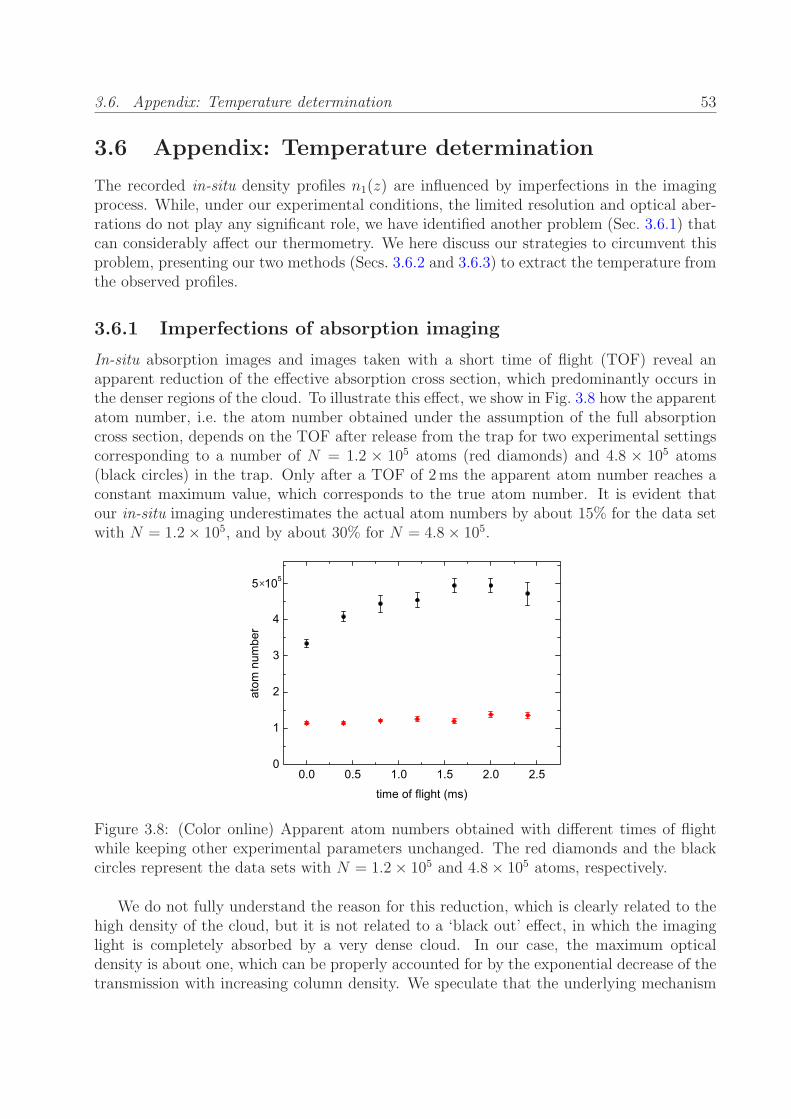
3.6. Appendix: Temperature determination 53
3.6 Appendix: Temperature determination
The recorded in-situ density profiles n1(z) are influenced by imperfections in the imagingprocess. While, under our experimental conditions, the limited resolution and optical aber-rations do not play any significant role, we have identified another problem (Sec. 3.6.1) thatcan considerably affect our thermometry. We here discuss our strategies to circumvent thisproblem, presenting our two methods (Secs. 3.6.2 and 3.6.3) to extract the temperature fromthe observed profiles.
3.6.1 Imperfections of absorption imaging
In-situ absorption images and images taken with a short time of flight (TOF) reveal anapparent reduction of the effective absorption cross section, which predominantly occurs inthe denser regions of the cloud. To illustrate this effect, we show in Fig. 3.8 how the apparentatom number, i.e. the atom number obtained under the assumption of the full absorptioncross section, depends on the TOF after release from the trap for two experimental settingscorresponding to a number of N = 1.2 × 10⁵ atoms (red diamonds) and 4.8 × 10⁵ atoms(black circles) in the trap. Only after a TOF of 2ms the apparent atom number reaches aconstant maximum value, which corresponds to the true atom number. It is evident thatour in-situ imaging underestimates the actual atom numbers by about 15% for the data setwith N = 1.2× 10⁵, and by about 30% for N = 4.8× 10⁵.
×
Figure 3.8: (Color online) Apparent atom numbers obtained with different times of flightwhile keeping other experimental parameters unchanged. The red diamonds and the blackcircles represent the data sets with N = 1.2× 10⁵ and 4.8× 10⁵ atoms, respectively.
We do not fully understand the reason for this reduction, which is clearly related to thehigh density of the cloud, but it is not related to a ‘black out’ effect, in which the imaginglight is completely absorbed by a very dense cloud. In our case, the maximum opticaldensity is about one, which can be properly accounted for by the exponential decrease of thetransmission with increasing column density. We speculate that the underlying mechanism
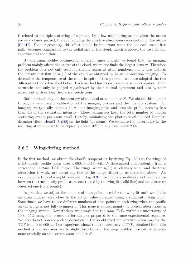
54 Chapter 3. Higher-nodal collective modes
is related to multiple scattering of a photon by a few neighboring atoms when the atomsare very closely packed, thereby reducing the effective absorption cross section of the atoms[Cho12]. For our geometry, this effect should be important when the photon’s ‘mean freepath’ becomes comparable to the radial size of the cloud, which is indeed the case for ourexperimental conditions.
By analyzing profiles obtained for different times of flight we found that the imagingproblem mainly affects the center of the cloud, where one finds the largest density. Thereforethe problem does not only result in smaller apparent atom numbers, but it also distortsthe density distribution n1(z) of the cloud as obtained by in-situ absorption imaging. Todetermine the temperature of the cloud in spite of this problem, we have adopted the twodifferent methods described below. Each method has its own systematic uncertainties. Theiraccuracies can only be judged a posteriori by their mutual agreement and also by theiragreement with certain theoretical predictions.
Both methods rely on the accuracy of the total atom number N . We obtain this numberthrough a very careful calibration of the imaging process and the imaging system. Forimaging, we typically adopt a 10-µs-long imaging pulse and keep the probe intensity lessthan 4% of the saturation intensity. These parameters keep the total number of photonscattering events per atom small, thereby minimizing the photon-recoil-induced Doppler-detuning effect [Hem81, Gri88] on the light 6Li atoms. We estimate the uncertainty in theresulting atom number to be typically about 10%, in any case below 20%.
3.6.2 Wing-fitting method
In the first method, we obtain the cloud’s temperature by fitting Eq. (3.9) to the wings ofa 1D density profile taken after a 600µs TOF, with N determined independently from acorresponding 2-ms TOF image. The wings, where n1(z) is relatively small and the totalabsorption is weak, are essentially free of the image distortion as described above. Anexample for a typical wing fit is shown in Fig. 3.9. The Figure also illustrates the differencebetween the true density profile as reconstructed by the wing fit (solid line) and the distortedobserved one (data points).
In practice, we adjust the number of data points used for the wing fit until we obtainan atom number very close to the actual value obtained using a sufficiently long TOF.Sometimes, we have to use different numbers of data points in each wing when the profileon the wings is not fully symmetric. This issue is caused mainly by optical aberrations inthe imaging system. Nevertheless, we always find the same T/TF within an uncertainty of10 to 15% using this procedure for samples prepared by the same experimental sequence.We also do not observe a clear deviation in the so obtained temperature when varying theTOF from 0 to 600µs. Our experience shows that the accuracy of T/TF obtained from thismethod is not very sensitive to slight distortions in the wing profiles. Instead, it dependsmore crucially on the correct atom number N .
3.6. Appendix: Temperature determination 55
-400 -200 0 200 4000.0
0.5
1.0
1.5
n1 (1
03 m
-1)
position ( m)
Figure 3.9: (Color online) Typical fit to the wings of the 1D density distribution to determineT/TF from Eq. (3.9). The filled circles represent the data used for fitting, and the solid line isthe full profile according to the fit. The open circles represent the remaining data that werenot used in the fit because of the problem to determine the correct linear density in the centerof the cloud. Here a TOF of 600µs was applied, the total atom number is N = 4.2 × 10⁵,and the temperature is T/TF = 0.36.
3.6.3 Potential-energy method
In the second method, we characterize the temperature in a model-independent way that doesnot require any a priori knowledge of the EOS. Based on the virial theorem [Tho05] we canobtain the total energy E of the harmonically trapped cloud from its potential energy, whichcan be calculated from the 1D density profile n1(z) according to E = 3mω2
z
∫
∞
−∞n1(z)z
2 dz.We define a dimensionless parameter E/E0, where E is normalized to the energy of a non-interacting, zero-temperature Fermi gas with the same number of atoms, E0 =
34NkBT .
To obtain an accurate value for E/E0 it is essential to have accurate knowledge of n1(z).Here we overcome the above-discussed distortion problem by ‘reconstructing’ the correctprofile. We measure the density profiles of the cloud for two different times of flight, 600-µsand 2ms. The corresponding profiles n1(z, 600µs) and n1(z, 2ms) provide complementaryinformation. While the 600-µs profile provides accurate information on the wings, it under-estimates the central part of the cloud. In contrast, the 2-ms profile suffers in the wingsfrom the expansion, but gives accurate information on the central part of the cloud. Withan appropriate algorithm to combine this information we can reconstruct the full profilewith reasonable accuracy. The reconstructed profile shows approximately the correct atomnumber and it maintains the wing distribution, which has large weights ∝ z2 in the totalenergy E.
We can now convert E/E0 into T/TF using the EOS from Ref. [Ku12]; for a relateddiscussion see Ref. [Cao11b]. Using the universal thermodynamic relations of a resonantlyinteracting Fermi gas, one can show that E/E0 is related to the x0 = βµ0 at the center of
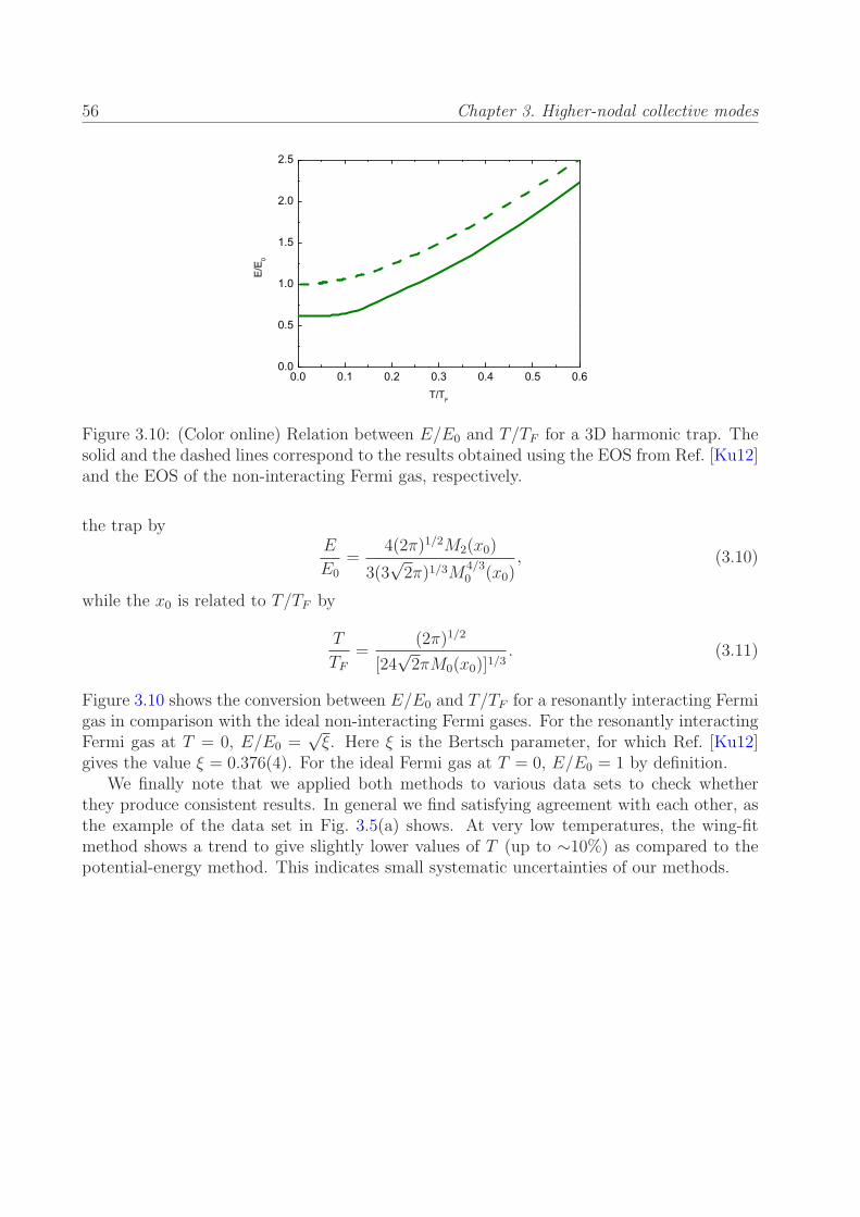
56 Chapter 3. Higher-nodal collective modes
0.0 0.1 0.2 0.3 0.4 0.5 0.60.0
0.5
1.0
1.5
2.0
2.5
E/E
0
T/TF
Figure 3.10: (Color online) Relation between E/E0 and T/TF for a 3D harmonic trap. Thesolid and the dashed lines correspond to the results obtained using the EOS from Ref. [Ku12]and the EOS of the non-interacting Fermi gas, respectively.
the trap byE
E0
=4(2π)1/2M2(x0)
3(3√2π)1/3M
4/30 (x0)
, (3.10)
while the x0 is related to T/TF by
T
TF=
(2π)1/2
[24√2πM0(x0)]1/3
. (3.11)
Figure 3.10 shows the conversion between E/E0 and T/TF for a resonantly interacting Fermigas in comparison with the ideal non-interacting Fermi gases. For the resonantly interactingFermi gas at T = 0, E/E0 =
√ξ. Here ξ is the Bertsch parameter, for which Ref. [Ku12]
gives the value ξ = 0.376(4). For the ideal Fermi gas at T = 0, E/E0 = 1 by definition.We finally note that we applied both methods to various data sets to check whether
they produce consistent results. In general we find satisfying agreement with each other, asthe example of the data set in Fig. 3.5(a) shows. At very low temperatures, the wing-fitmethod shows a trend to give slightly lower values of T (up to ∼10%) as compared to thepotential-energy method. This indicates small systematic uncertainties of our methods.
Chapter 4
Publication: Collective Modes in a
Unitary Fermi Gas across the
Superfluid Phase Transition†
Phys. Rev. Lett 110, 055303 (2013)
Meng Khoon Tey, Leonid A. Sidorenkov, Edmundo R. Sanchez Guajardo,and Rudolf Grimm
Institut fur Quantenoptik und Quanteninformation (IQOQI), Osterreichische Akademie der Wissenschaftenand Institut fur Experimentalphysik und Zentrum fur Quantenphysik, Universitat Innsbruck, 6020
Innsbruck, Austria
Mark J. H. Ku, and Martin W. Zwierlein
MIT-Harvard Center for Ultracold Atoms, Research Laboratory of Electronics,and Department of Physics, Massachusetts Institute of Technology, Cambridge, Massachusetts 02139, USA
Yan-Hua Hou,1 Lev Pitaevskii,1,2 and Sandro Stringari1
1Dipartimento di Fisica, Universita di Trento and INO-CNR BEC Center, I-38123 Povo, Italy2Kapitza Institute for Physical Problems RAS, Kosygina 2, 119334 Moscow, Russia
†The author of the present thesis performed the measurements, together with M.K.T. and E.R.S.G.,under the supervision of R.G. The data analysis was carried out by M.K.T. and the author. Theoreticalsupport was provided by Y.-H.H, L.P. and S.S. The data on equation of state were provided by M.J.H.K.and M.W.Z.
57
58 Chapter 4. Collective modes across the superfluid phase transition
We provide a joint theoretical and experimental investigation of the tempera-ture dependence of the collective oscillations of first sound nature exhibited by ahighly elongated harmonically trapped Fermi gas at unitarity, including the re-gion below the critical temperature for superfluidity. Differently from the lowestaxial breathing mode, the hydrodynamic frequencies of the higher nodal excita-tions show a temperature dependence, which is calculated starting from Landautwo-fluid theory and using the available experimental knowledge of the equationof state. The experimental results agree with high accuracy with the predictionsof theory and provide the first evidence for the temperature dependence of thecollective frequencies near the superfluid phase transition.
Collective oscillations provide powerful tools to understand the physical behavior of quan-tum many-body systems from different points of view and to test fundamental theories. Onthe one hand, collective modes can be used to explore different dynamical regimes of thesystem, such as superfluid, collisional, or collisionless regimes, for both Bose and Fermistatistics [Pit03, Ing08, Gio08, Blo08]. On the other hand, the mode frequencies allow toprobe the equation of state (EOS) of the system, including its temperature dependence.Major benefits result from the high accuracies attainable in the measurements of collectivefrequencies, which often enable refined investigations of subtle interaction effects.
The many-body physics of unitary Fermi gases, i.e. two-component Fermi gases withinfinite scattering length, has attracted tremendous interest over the last decade [Ing08,Gio08, Blo08]. The unitary Fermi gas is characterized by strong interaction effects in theEOS [Kin05b, Hor10, Nas10, Ku12] and reveals a unique universal thermodynamic behavior[Ho04]. Furthermore, at finite temperature, the strong interactions favor the collisionalhydrodynamic regime, differently from the common situation in weakly interacting Bosegases. The low-frequency modes of a harmonically trapped Fermi gas have been the subjectof intensive experimental [Kin04a, Bar04a, Alt07b] and theoretical (see [Gio08] and referencestherein) efforts. The temperature dependence has been studied in Refs. [Kin05a, Wri07,Rie08]. Remarkably, at unitarity all modes observed so far turned out to be insensitiveto the different nature of a superfluid and a classical gas, with their frequencies remainingindependent of temperature throughout the hydrodynamic regime. Previous experimentshave demonstrated the crossover from hydrodynamic to collisionless behavior, which typicallyoccurs for temperatures approaching the Fermi temperature, without giving any furtherinformation on the regime of lower temperatures where the gas is deeply hydrodynamic andthe superfluid phase transition occurs.
In this Letter, we report a joint effort of theory and experiment on higher-nodal collectivemodes in the unitary Fermi gas. We present a 1D hydrodynamic approach to describe axialmodes in a trapped ‘cigar-shaped’ cloud. Our experimental results confirm the predictedintrinsic sensitivity of higher-nodal modes to the EOS in the low-temperature regime, aboveand even well below the superfluid phase transition.
The macroscopic dynamic behavior of a superfluid is governed by the Landau two-fluidhydrodynamic equations [Kha65] holding in the deep collisional regime ωτ ≪ 1 where τ is atypical collisional time and ω is the frequency of the relevant sound mode in the trap. Lan-dau’s equations consist of the equation of continuity for the total density, the equation for the
59
velocity of the superfluid component, the equation for the entropy density and the equationfor the current density. The physical ingredients entering these equations are the equationof state and the superfluid density. At zero temperature they reduce to the irrotationalhydrodynamic equations of superfluids, above the critical point to the usual hydrodynamicequations of normal fluids. Below Tc these equations describe the propagation of first andsecond sound, the former being basically a density wave, with the normal and superfluidcomponents moving in phase, the latter being a temperature or entropy wave. For weaklycompressible fluids the coupling between first and second sound is small [Kha65]. This isthe case of superfluid helium and also of the unitary Fermi gas [Tay09]. Since in the presentwork we investigate the collective oscillations of density (first sound), we simplify the searchfor the solutions of Landau’s equation by requiring that the velocity fields of the normal andsuperfluid components are equal. Under this approximation the equations of motion involveonly the EOS, the superfluid density playing a role only in the propagation of second sound.
In the presence of a trapping potential, the solution of Landau’s equations is highly non-trivial, due to the inhomogeneity of the density profile, and has been so far calculated onlyfor the simplest case of isotropic trapping [He07, Tay09]. Since the experimental excita-tion and observation of these modes are more easily accessible with very elongated traps, inthe following we focus on such configurations. In [Ber10] it was shown that under suitableconditions of radial trapping one can derive simplified 1D hydrodynamic equations startingfrom the more general 3D Landau’s equations. The basic point for such a derivation is theassumption that both the velocity field vz along the long axis and the temperature fluctua-tions during the propagation of sound do not depend on the radial coordinates. This 1D likehydrodynamic formulation is justified under the condition that the viscosity and the thermalconductivity are sufficiently large to ensure, respectively, the absence of radial gradients inthe velocity vz and the temperature. The condition for the viscosity can be recast in the formη ≫ ρn1ω where ρn1 is the normal 1D mass density, obtained by radial integration of the 3Dnormal density. An analogous condition holds for the thermal conductivity. These conditionsare better satisfied in the presence of tight radial confinement and for the lowest frequencyoscillations. One can estimate the values of shear viscosity η using the experimental data of[Cao11b]. For the actual conditions of our experiments both sides of the inequality are ofthe same order of magnitude and consequently the full applicability of the 1D hydrodynamicformulation can be justified only a posteriori. Violation of the 1D condition would result ina damping of the collective oscillations so that, to the extent that the observed damping issmall, we expect that the assumption of velocity field and temperature being independentof the radial coordinate is a reasonable ansatz for our variational approach.
Under the above assumptions and focusing on the unitary Fermi gas, the equation forthe velocity field, characterizing the density oscillations of the gas in a highly elongatedharmonic trap, takes the form (see [Hou13b] for a complete and systematic derivation):
m(ω2 − ω2z)vz −
7
5mω2
zz∂zvz +7
5
P1
n1
∂2zvz = 0 (4.1)
where we have considered oscillations in time proportional to e−iωt. Here, ωz representsthe trap frequency along the axial direction z, and m is the atom’s mass. Eq.(4.1) ex-plicitly points out the crucial role played by the equation of state P1(n1, T ), where P1 =

60 Chapter 4. Collective modes across the superfluid phase transition
∫
Pdxdy is the “1D pressure” (having units of force) and n1 =∫
ndxdy is the atom numberper unit length. In order to derive Eq.(4.1) we have explicitly used the adiabatic resultn1 (∂P1/∂n1)s1 = 7/5P1 holding at unitarity at all temperatures, where s1 = (1/n1)
∫
sdxdyis the entropy per atom with s the entropy density and we have assumed the validity of thelocal density approximation along both the axial and radial directions.
At zero temperature and in the classical limit of high temperature the hydrodynamicequation (4.1) admits analytic solutions of polynomial form vz = akz
k + ak−2zk−2 + ..., with
integer values of k. At T = 0, where P1(n1)/n1 = (2/7)(µ0 − (1/2)mω2zz
2), with µ0 thechemical potential at the center of the trap, the frequency of the k-th mode is given by
ω2 =1
5(k + 1)(k + 5)ω2
z . (4.2)
In the classical limit, where P1/n1 = kBT , one finds the different k dependence
ω2 =1
5(7k + 5)ω2
z . (4.3)
It is worth noticing that Eqs. (4.2) and (4.3) coincide for k = 0 (center of mass oscillation)and k = 1 (lowest axial breathing mode), while they predict different values for the highernodal solutions. One can actually prove that not only the frequency of the center of massbut, at unitarity, also the frequency of the lowest axial breathing mode is independentof temperature, corresponding to an exact scaling solution of the two fluid hydrodynamicequations [Hou13b]. It then follows that only the k ≥ 2 modes exhibit a temperaturedependence.
In order to provide a simple quantitative prediction for the temperature dependenceof the mode frequencies, we have developed a variational approach to the solution of thehydrodynamic equation (4.1) with the ansatz vz = a2z
2 + a0 for the k = 2 mode. Thisansatz reproduces exactly the frequency of the k = 2 mode in the limits of T = 0 and highT . For intermediate temperatures we obtain [Hou13b]
ω2k=2 =
129t2 − 25
5(9t2 − 5)ω2z , (4.4)
where t2 =M0M4/M22 . We have introduced the dimensionless moments
Mℓ =
∫ βµ0
−∞
dx(βµ0 − x)(ℓ+1)/2n(x)λ3T (4.5)
of the 3D number density n(x), where x is the local chemical potential times β = 1/kBTand λT is the thermal de Broglie wavelength. The temperature dependence of the momentsMℓ can be evaluated using the experimentally determined EOS [Ku12]. Approaching theclassical regime, for βµ . −1.5, the virial expansion of the EOS [Liu09] holds [Ku12] andallows to extend the integral to βµ→ −∞. At low temperatures, corresponding to βµ > 4,the EOS is governed by phonons and is solely determined by the Bertsch parameter ξ. Theerror of the quantity t2 above resulting from the error in the density EOS is less than 1%.We have checked that our variational predictions are practically indistinguishable from the

61
exact numerical solution of Eq. (4.1). Starting from the equation of continuity one can alsocalculate the shape of the density oscillations of each mode, proportional to ∂z(n1vz).
Experimentally, we prepare an ultracold, resonantly interacting Fermi gas by evaporatinga two-component spin mixture of fermionic 6Li in an optical dipole trap [Joc03b]. The atomiccloud contains typically N/2 = 1.5× 10⁵ atoms per spin state, and the magnetic field is setto 834G, right on top of the well-known broad Feshbach resonance [Chi10]. For the lowesttemperatures, the trapping beam (wavelength 1075 nm) has a waist of 31 µm, the trapdepth is about 2µK, and the axial and radial trap frequencies are ωz = 2π×22.52(2)Hz andωr = 2π × 473(2)Hz, respectively. For experiments at higher temperatures, the beam waistis increased to 38 µm, and deeper traps are used (up to 16µK depth) with trap frequenciesof up to ωz = 2π × 23.31(3)Hz and ωr = 2π × 1226(6)Hz. The corresponding Fermitemperatures TF = ~(3Nω2
rωz)1/3/kB vary between about 0.8 and 1.5µK. We point out that
essentially perfect harmonic confinement along the long trap axis (z-axis) is ensured by themagnetic trapping that results from the curvature of the magnetic field used for Feshbachtuning [Joc03b]. Also anharmonicities in the radial confinement remain negligibly small. Toprobe the ultracold gas we record one-dimensional axial density profiles n1(z) by near in-situabsorption imaging [SG13].
The temperature T of the gas is set by controlled heating, always starting from a deeplycooled cloud (T/TF ≈ 0.1). In the low temperature range (T . 0.2TF ), we simply introducea variable hold time of up to 4 s in which residual trap heating slowly increases T . Highertemperatures are reached by parametric heating, modulating the trap power at about 2ωr,and introducing a sufficient hold time to reach thermal equilibrium between the differentdegrees of freedom. We characterize the resulting temperature in a model-independent waythat does not require any a priori knowledge of the EOS. Based on the virial theorem[Tho05] we introduce the dimensionless parameter E/E0, which represents the total energyE = 3mω2
z
∫
∞
−∞dzz2n1(z) normalized to the energy of a noninteracting, zero-temperature
Fermi gas, E0 = 34NkBTF . For a given EOS, the energy scale (E/E0) can be converted
to a temperature scale (T/TF ). Alternatively, we obtain the cloud’s temperature by fittingthe experimental profiles n1(z) with T -dependent theoretical profiles [Ho10, Nas10]. Forboth methods, we apply the EOS according to Ref. [Ku12]. We note that the temperaturesobtained by both methods in general show satisfying agreement with each other. At verylow temperatures the latter method shows a trend to give slightly lower values of T (up to∼10%), which indicates small systematic uncertainties of our measurements.
We selectively excite axial modes of order k by using a resonant excitation scheme.As illustrated in Fig. 4.1(a), a repulsive 532-nm laser beam perpendicularly intersects thetrapping beam, with its position and size chosen in a way to provide best mode matching.Typically, the excitation pulse contains 8 cycles of sinusoidal modulation with a half-cyclesine envelope, and the maximum potential height of the excitation beam is kept to about0.01 kBTF . The power, length and shape of the excitation pulse are optimized in order toresonantly drive the desired small-amplitude oscillation. The amplitude of the correspondingdensity modulation stays well below 3% of the central density of the cloud.
We record axial density profiles n1(z, t) of the excited cloud for various time delays tafter the excitation pulse. We then perform a Fast Fourier Transform (FFT). The resultingfunction n(z, ω) reveals the collective mode spectrum with eigenfrequencies ωk and the corre-
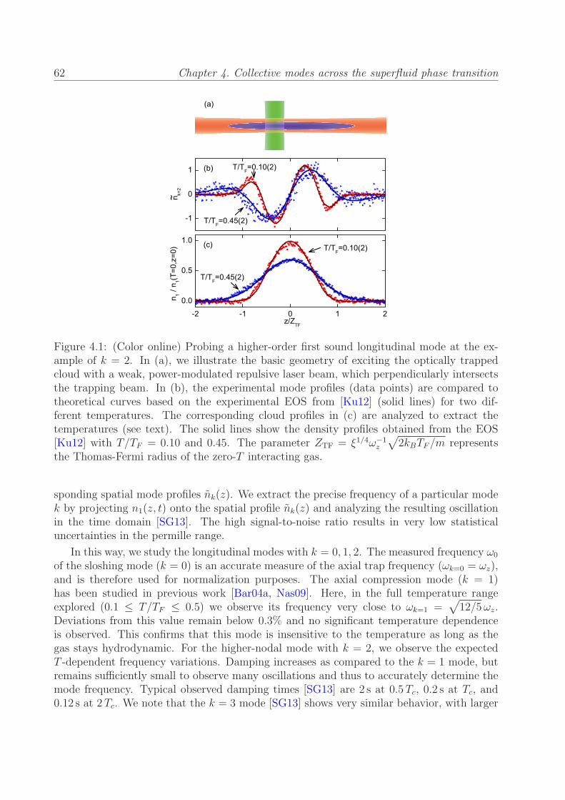
62 Chapter 4. Collective modes across the superfluid phase transition
~
(a)
Figure 4.1: (Color online) Probing a higher-order first sound longitudinal mode at the ex-ample of k = 2. In (a), we illustrate the basic geometry of exciting the optically trappedcloud with a weak, power-modulated repulsive laser beam, which perpendicularly intersectsthe trapping beam. In (b), the experimental mode profiles (data points) are compared totheoretical curves based on the experimental EOS from [Ku12] (solid lines) for two dif-ferent temperatures. The corresponding cloud profiles in (c) are analyzed to extract thetemperatures (see text). The solid lines show the density profiles obtained from the EOS[Ku12] with T/TF = 0.10 and 0.45. The parameter ZTF = ξ1/4ω−1
z
√
2kBTF/m representsthe Thomas-Fermi radius of the zero-T interacting gas.
sponding spatial mode profiles nk(z). We extract the precise frequency of a particular modek by projecting n1(z, t) onto the spatial profile nk(z) and analyzing the resulting oscillationin the time domain [SG13]. The high signal-to-noise ratio results in very low statisticaluncertainties in the permille range.
In this way, we study the longitudinal modes with k = 0, 1, 2. The measured frequency ω0
of the sloshing mode (k = 0) is an accurate measure of the axial trap frequency (ωk=0 = ωz),and is therefore used for normalization purposes. The axial compression mode (k = 1)has been studied in previous work [Bar04a, Nas09]. Here, in the full temperature rangeexplored (0.1 ≤ T/TF ≤ 0.5) we observe its frequency very close to ωk=1 =
√
12/5ωz.Deviations from this value remain below 0.3% and no significant temperature dependenceis observed. This confirms that this mode is insensitive to the temperature as long as thegas stays hydrodynamic. For the higher-nodal mode with k = 2, we observe the expectedT -dependent frequency variations. Damping increases as compared to the k = 1 mode, butremains sufficiently small to observe many oscillations and thus to accurately determine themode frequency. Typical observed damping times [SG13] are 2 s at 0.5Tc, 0.2 s at Tc, and0.12 s at 2Tc. We note that the k = 3 mode [SG13] shows very similar behavior, with larger
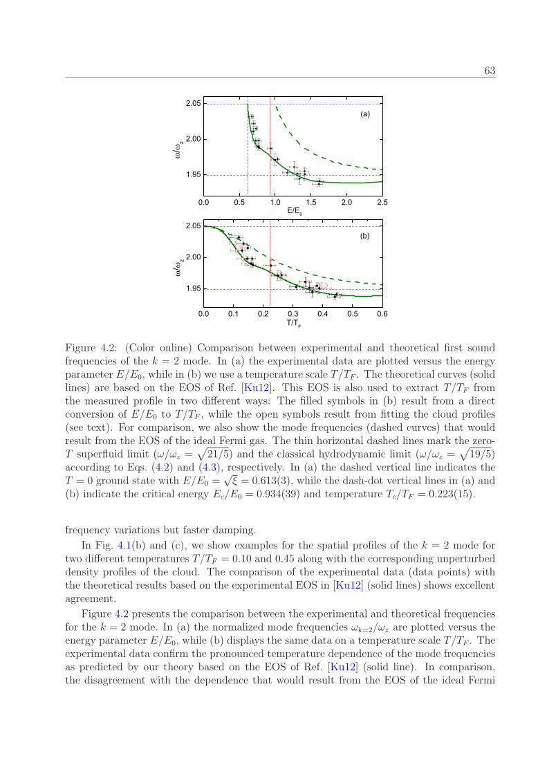
63
Figure 4.2: (Color online) Comparison between experimental and theoretical first soundfrequencies of the k = 2 mode. In (a) the experimental data are plotted versus the energyparameter E/E0, while in (b) we use a temperature scale T/TF . The theoretical curves (solidlines) are based on the EOS of Ref. [Ku12]. This EOS is also used to extract T/TF fromthe measured profile in two different ways: The filled symbols in (b) result from a directconversion of E/E0 to T/TF , while the open symbols result from fitting the cloud profiles(see text). For comparison, we also show the mode frequencies (dashed curves) that wouldresult from the EOS of the ideal Fermi gas. The thin horizontal dashed lines mark the zero-T superfluid limit (ω/ωz =
√
21/5) and the classical hydrodynamic limit (ω/ωz =√
19/5)according to Eqs. (4.2) and (4.3), respectively. In (a) the dashed vertical line indicates theT = 0 ground state with E/E0 =
√ξ = 0.613(3), while the dash-dot vertical lines in (a) and
(b) indicate the critical energy Ec/E0 = 0.934(39) and temperature Tc/TF = 0.223(15).
frequency variations but faster damping.
In Fig. 4.1(b) and (c), we show examples for the spatial profiles of the k = 2 mode fortwo different temperatures T/TF = 0.10 and 0.45 along with the corresponding unperturbeddensity profiles of the cloud. The comparison of the experimental data (data points) withthe theoretical results based on the experimental EOS in [Ku12] (solid lines) shows excellentagreement.
Figure 4.2 presents the comparison between the experimental and theoretical frequenciesfor the k = 2 mode. In (a) the normalized mode frequencies ωk=2/ωz are plotted versus theenergy parameter E/E0, while (b) displays the same data on a temperature scale T/TF . Theexperimental data confirm the pronounced temperature dependence of the mode frequenciesas predicted by our theory based on the EOS of Ref. [Ku12] (solid line). In comparison,the disagreement with the dependence that would result from the EOS of the ideal Fermi
64 Chapter 4. Collective modes across the superfluid phase transition
gas (dashed line) highlights the important role of the EOS. At the lowest temperatures(T/TF ≈ 0.1) the frequency lies close to the T = 0 superfluid limit, but already shows asignificant down-shift amounting to almost 1%. At the highest temperatures (T/TF ≈ 0.45)our data show a clear trend to go below the asymptotic high-temperature value, i.e. theclassical hydrodynamic limit. The corresponding non-monotonic temperature dependencecan be understood based on the first-order correction to the EOS resulting from the virialexpansion at high temperatures.
In conclusion, our combined theoretical and experimental work on higher-nodal axialcollective modes of a unitary Fermi gas reveals a pronounced temperature dependence be-low and near the superfluid phase transition. The observed temperature dependence is aunique feature of higher nodal modes, not present for any other collective mode studiedin Fermi gases so far. Our theoretical approach is based on a 1D two-fluid hydrodynamicmodel describing the frequently used elongated ‘cigar-shaped’ trap geometry. The excellentagreement with the experimental results provides a stringent test for the validity of this1D approach and highlights its potential power to accurately describe second sound modes.Moreover, our measurements provide an independent confirmation of the recently measuredEOS of a unitary Fermi gas.
We would like to thank John Thomas for useful discussions and Florian Schreck fordiscussion and experimental support. The Innsbruck team acknowledges support from theAustrian Science Fund (FWF) within SFB FoQuS (project No. F4004-N16). The Trentoteam acknowledges support from the European Research Council through the project QGBE.The MIT work was supported by the NSF, AFOSR, ONR, ARO with funding from theDARPA OLE program, and the David and Lucile Packard Foundation.

Chapter 5
Publication: Second sound and the
superfluid fraction in a resonantly
interacting Fermi gas†
accepted for publication in Nature (2013)
Leonid A. Sidorenkov1,2, Meng Khoon Tey1,2, Rudolf Grimm1,2, Yan-Hua Hou3, LevPitaevskii3,4, Sandro Stringari3
1Institut fur Quantenoptik und Quanteninformation (IQOQI), Osterreichische Akademie derWissenschaften, 6020 Innsbruck, Austria
2Institut fur Experimentalphysik und Zentrum fur Quantenphysik, Universitat Innsbruck, 6020 Innsbruck,Austria
3Dipartimento di Fisica, Universita di Trento and INO-CNR BEC Center, I-38123 Povo, Italy4Kapitza Institute for Physical Problems RAS, Kosygina 2, 119334 Moscow, Russia
†The author of the present thesis developed the experimental procedure, performed the measurements andanalysed the data, together with M.K.T., under the supervision of R.G. Theoretical support was providedby Y.-H.H, L.P. and S.S.
65

66 Chapter 5. Second sound and the superfluid fraction
Superfluidity is a macroscopic quantum phenomenon, which shows up belowa critical temperature [Kap38, All38] and leads to a peculiar behavior of matter,with frictionless flow, the formation of quantized vortices, and the quenchingof the moment of inertia being intriguing examples. A remarkable explanationfor many phenomena exhibited by a superfluid at finite temperature can begiven in terms of a two-fluid mixture [Tis38, Lan41] comprised of a normalcomponent that behaves like a usual fluid and a superfluid component withzero viscosity and zero entropy. Important examples of superfluid systems areliquid helium and neutron stars. More recently, ultracold atomic gases haveemerged as new superfluid systems with unprecedented possibilities to controlinteractions and external confinement. Here we report the first observation of‘second sound’ in an ultracold Fermi gas with resonant interactions. Secondsound is a striking manifestation of the two-component nature of a superfluidand corresponds to an entropy wave, where the superfluid and the non-superfluidcomponents oscillate in opposite phase, different from ordinary sound (‘firstsound’), where they oscillate in phase. The speed of second sound dependsexplicitly on the value of the superfluid fraction [Kha65], a quantity sensitive tothe spectrum of elementary excitations [Lan47]. Our measurements allow us toextract the temperature dependence of the superfluid fraction, which in stronglyinteracting quantum gases has been an inaccessible quantity so far.
5.1 Main results
Second sound was first measured in liquid helium II (superfluid 4He below 2.2K), whichrepresents the paradigm of quantum liquids characterized by strong interactions [Atk59].For the description of this system and its peculiar properties Landau developed his theory oftwo-fluid hydrodynamics [Lan41]. In liquid helium II, second sound can be generated [Pes44]by local time-dependent heating and detected by observing the propagation of the resultingtemperature wave. In this original context, second sound is characterized as a wave thatpropagates at constant pressure (isobaric oscillation), in contrast to first sound being a wavethat propagates at constant entropy per particle (adiabatic oscillation), just like ordinarysound.
The observation of second sound in ultracold atomic quantum gases has been a long-standing goal. In weakly interacting Bose-Einstein condensed gases, second sound behavesquite differently from the case of liquid helium II. In these systems, the superfluid densitycoincides with the density of the Bose-Einstein condensed component and, in the experimen-tally relevant temperature range, second sound reduces to an oscillation of the condensate,the thermal component remaining essentially at rest. The corresponding temperature de-pendence of the speed of sound was measured in Ref. [Mep09a]. In two other experiments[SK98, Mep09b], the relative motion of the condensate and the thermal component was in-vestigated and frequency shifts and damping effects were observed. In contrast to diluteBose gases, resonantly interacting Fermi gases [Gio08, Blo08] are characterized by effectsof strong interactions. In such systems, superfluidity and the universal thermodynamics
5.1. Main results 67
[Ho04, Kin05b, Hor10, Nas10, Ku12] have been subjects of intense research. Here the nor-mal component behaves in a deeply hydrodynamic way in a wide range of temperatures andthe spatial overlap between the normal and the superfluid components can be very large alsoin the presence of harmonic trapping. In this favorable situation, Landau’s two-fluid theorycan be readily applied, which suggests a behavior similar to superfluid helium, including theoccurrence of second sound.
Our system is an ultracold, superfluid sample of fermionic 6Li atoms, prepared in ahighly elongated harmonic trapping potential (Methods) by well-established procedures oflaser and evaporative cooling [Tey13]. The sample consists of N = 3.0 × 10⁵ atoms in abalanced mixture of the two lowest spin states, and is about 500µm long and 20µm wide. Itis characterized by the Fermi temperature T trap
F ≈ 0.9µK (Methods). A magnetic bias fieldof 834G is applied, which tunes the interaction between the two spin components right ontop of an s-wave scattering length resonance (‘unitarity limit’ of interactions). The cloud’stemperature T is determined by analyzing axial density profiles [Nas10, Tey13], using theknowledge of the equation of state (EOS) from Ref. [Ku12]. The relevant temperature rangefor the present experiments is between 0.11 and 0.15T trap
F .
Our method for observing sound propagation builds on the classical scheme to detect thepropagation of first sound in Bose-Einstein condensates [And97a], which was also appliedto resonantly interacting Fermi gases [Jos07]. The general idea is to prepare the quantumgas in a trap that is highly elongated, to create a local perturbation, and to detect its one-dimensional propagation as a pulse along the long trap axis. In the case of first sound, boththe creation and the detection of such an excitation are straightforward, while being lessobvious for second sound.
For the local excitation of the cloud, we use a repulsive dipole potential created by atightly focussed green laser beam (Methods) that perpendicularly intercepts the trappedsample in its center, as shown in Fig. 1a. To excite first sound, we suddenly turn on therepulsive beam. The local reduction of the trapping potential acts on the superfluid andnormal component in the same way and creates a small hump in the axial density distribu-tion. To excite second sound, we keep the green beam’s power constant during the wholeexperimental sequence with the exception of a short power-modulation burst, which contains8 sinusoidal oscillations in 4.5 ms (Methods and Supplementary Information). The fast mod-ulation locally drives the system out of equilibrium and the following relaxation increasesentropy and temperature. The duration of the burst is chosen such that the system canestablish a local thermal equilibrium on a length scale that covers the transverse cloud size,but is much shorter than the axial extension of the cloud. In all cases, we take care thatthe excitation remains a small perturbation of the whole system, which globally stays in athermal equilibrium state.
For detection we record the axial density profile n1(z, t) for various time delays t after theexcitation pulse, where n1(z, t) is the number density integrated over the transverse degreesof freedom. To enhance the visibility of the density perturbation, we subtract a backgroundprofile n1(z) obtained by averaging the profiles over all measured delay times. Our signalδn1(z, t) = n1(z, t)− n1(z) is finally normalized to the maximum observed density n1,max.
The key point for the detection of second sound is the coupling [Ara09, Hu10] betweentemperature and density variations, which occurs in a systems exhibiting thermal expansion.

68 Chapter 5. Second sound and the superfluid fraction
0
10
20
Tim
e (m
s)
b
0 4000
10
20
30
Position (mm)
Tim
e (m
s)
c
a
+0.09
+0.06
Figure 5.1: Observing the propagation of first and second sound. a, The basicgeometry of exciting the optically trapped cloud with a weak, power-modulated repulsivelaser beam (green), which perpendicularly intersects the trapping beam (red). The trappedcloud has a superfluid core (|z| < 200µm), surrounded by a normal region (about 1.5 timeslarger). b and c, Normalized differential axial density profiles δn1(z, t)/n1,max taken forvariable delay times after the excitation show the propagation of first sound (local densityincrease, bright) and second sound (local decrease, dark). The temperature of the atomiccloud is T = 0.135(10)T trap
F . The vertical dashed lines indicate the axial region wheresuperfluid is expected to exist according to a recent determination of the critical temperature[Ku12].
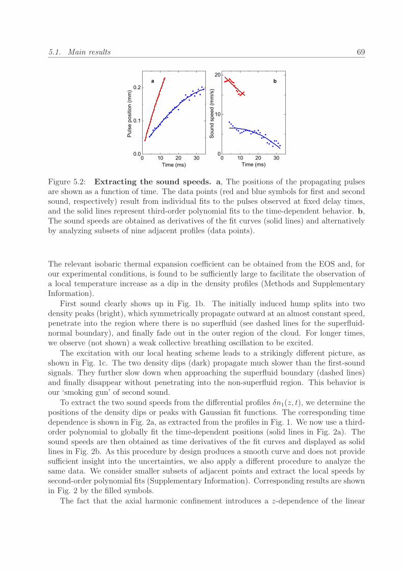
5.1. Main results 69
Figure 5.2: Extracting the sound speeds. a, The positions of the propagating pulsesare shown as a function of time. The data points (red and blue symbols for first and secondsound, respectively) result from individual fits to the pulses observed at fixed delay times,and the solid lines represent third-order polynomial fits to the time-dependent behavior. b,The sound speeds are obtained as derivatives of the fit curves (solid lines) and alternativelyby analyzing subsets of nine adjacent profiles (data points).
The relevant isobaric thermal expansion coefficient can be obtained from the EOS and, forour experimental conditions, is found to be sufficiently large to facilitate the observation ofa local temperature increase as a dip in the density profiles (Methods and SupplementaryInformation).
First sound clearly shows up in Fig. 1b. The initially induced hump splits into twodensity peaks (bright), which symmetrically propagate outward at an almost constant speed,penetrate into the region where there is no superfluid (see dashed lines for the superfluid-normal boundary), and finally fade out in the outer region of the cloud. For longer times,we observe (not shown) a weak collective breathing oscillation to be excited.
The excitation with our local heating scheme leads to a strikingly different picture, asshown in Fig. 1c. The two density dips (dark) propagate much slower than the first-soundsignals. They further slow down when approaching the superfluid boundary (dashed lines)and finally disappear without penetrating into the non-superfluid region. This behavior isour ‘smoking gun’ of second sound.
To extract the two sound speeds from the differential profiles δn1(z, t), we determine thepositions of the density dips or peaks with Gaussian fit functions. The corresponding timedependence is shown in Fig. 2a, as extracted from the profiles in Fig. 1. We now use a third-order polynomial to globally fit the time-dependent positions (solid lines in Fig. 2a). Thesound speeds are then obtained as time derivatives of the fit curves and displayed as solidlines in Fig. 2b. As this procedure by design produces a smooth curve and does not providesufficient insight into the uncertainties, we also apply a different procedure to analyze thesame data. We consider smaller subsets of adjacent points and extract the local speeds bysecond-order polynomial fits (Supplementary Information). Corresponding results are shownin Fig. 2 by the filled symbols.
The fact that the axial harmonic confinement introduces a z-dependence of the linear
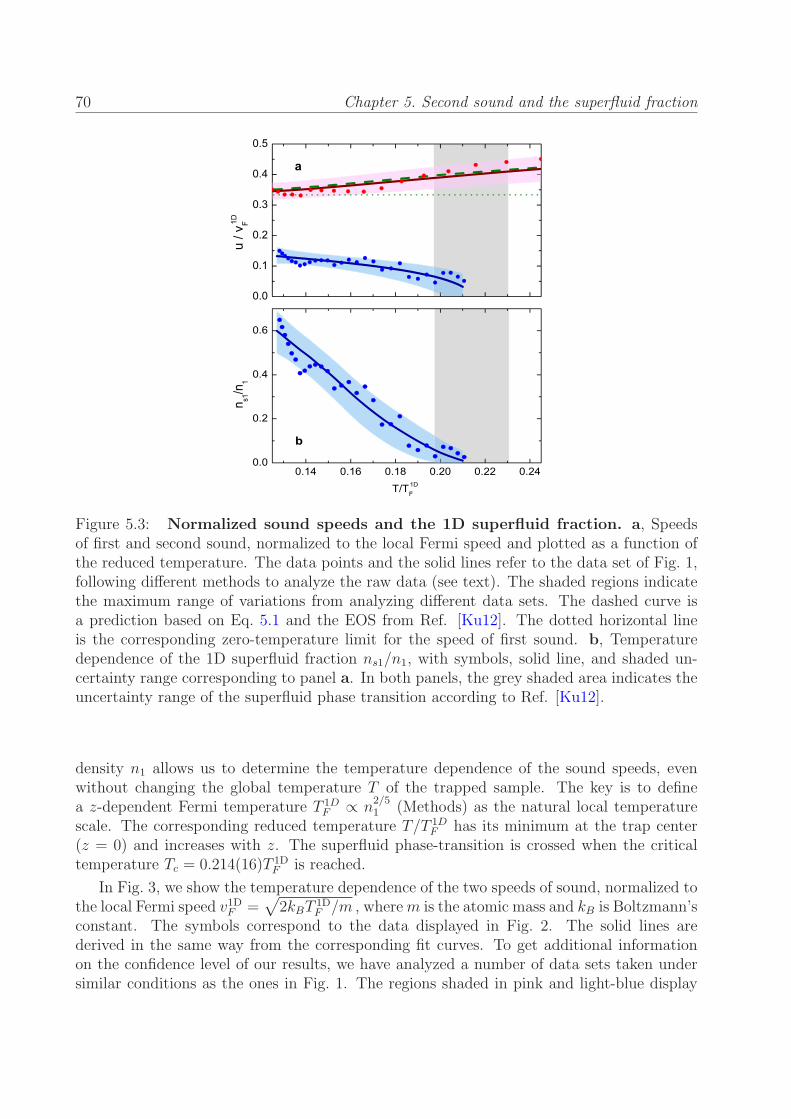
70 Chapter 5. Second sound and the superfluid fraction
Figure 5.3: Normalized sound speeds and the 1D superfluid fraction. a, Speedsof first and second sound, normalized to the local Fermi speed and plotted as a function ofthe reduced temperature. The data points and the solid lines refer to the data set of Fig. 1,following different methods to analyze the raw data (see text). The shaded regions indicatethe maximum range of variations from analyzing different data sets. The dashed curve isa prediction based on Eq. 5.1 and the EOS from Ref. [Ku12]. The dotted horizontal lineis the corresponding zero-temperature limit for the speed of first sound. b, Temperaturedependence of the 1D superfluid fraction ns1/n1, with symbols, solid line, and shaded un-certainty range corresponding to panel a. In both panels, the grey shaded area indicates theuncertainty range of the superfluid phase transition according to Ref. [Ku12].
density n1 allows us to determine the temperature dependence of the sound speeds, evenwithout changing the global temperature T of the trapped sample. The key is to definea z-dependent Fermi temperature T 1D
F ∝ n2/51 (Methods) as the natural local temperature
scale. The corresponding reduced temperature T/T 1DF has its minimum at the trap center
(z = 0) and increases with z. The superfluid phase-transition is crossed when the criticaltemperature Tc = 0.214(16)T 1D
F is reached.
In Fig. 3, we show the temperature dependence of the two speeds of sound, normalized tothe local Fermi speed v1DF =
√
2kBT 1DF /m , wherem is the atomic mass and kB is Boltzmann’s
constant. The symbols correspond to the data displayed in Fig. 2. The solid lines arederived in the same way from the corresponding fit curves. To get additional informationon the confidence level of our results, we have analyzed a number of data sets taken undersimilar conditions as the ones in Fig. 1. The regions shaded in pink and light-blue display

5.1. Main results 71
the maximum range of variations considering all our different data sets (SupplementaryInformation).
Our interpretation of the experimental results relies on an effective one-dimensional ap-proach that allows to solve Landau’s two-fluid hydrodynamic equations for a highly elongatedsystem [Ber10, Hou13b]. The basic assumptions are a thermal equilibrium in the radial di-rection and sufficient shear viscosity to establish a flow field that is independent of the radialposition. Within this theoretical framework and under the local density approximation, effec-tive 1D thermodynamic quantities can be defined by integration over the transverse degreesof freedom, such that a thermodynamic quantity q yields a 1D counterpart q1 ≡ 2π
∫
∞
0q r dr.
We can express the normalized speeds of first and second sound as
u1v1DF
=
√
7
10
P1
n1kBT 1DF
, (5.1)
and
u2v1DF
=
√
T
2kBT 1DF
s21cp1
ns1
nn1
, (5.2)
where P1 denotes the 1D pressure (unit of a force), s1 = s1/n1 is the entropy per particle,and cp1 = T (∂s1/∂T )p1 is the isobaric heat capacity per particle. These thermodynamicquantities can be calculated from the EOS as functions of the reduced temperature T/T 1D
F ,as we discuss in detail in Ref. [Hou13b]. The quantities ns1 and nn1 = n1 − ns1, whichrepresent the linear number densities of the superfluid and the normal component, cannotbe determined from the known EOS.
The speed of first sound provides us with an important benchmark for our experimentalmethod and the interpretation of the measurements in the 1D theoretical framework. Theexperimental results (red symbols and upper solid line in Fig. 3a) are in excellent agreementwith the calculation (dashed line) based on Eq. 5.1 and the EOS from Ref. [Ku12], which isa further confirmation for the validity of our theoretical approach in addition to the recentmeasurements of the T -dependent frequencies of higher-nodal collective modes [Tey13].
The measured speed of second sound (blue line and data points in Fig. 3a) is observed todecrease with temperature, in contrast to first sound. The general behavior fits very well tothe qualitative predictions in Ref. [Ber10]. We can now extract the 1D superfluid fractionns1/n1, which is the unknown quantity in Eq. 5.2. The result is presented in Fig. 3b, wherens1/n1 shows a smooth increase with decreasing T below the critical temperature.
We finally reconstruct (Methods) the temperature dependence of the superfluid fractionns/n for the homogeneous 3D case, which has been an inaccessible quantity so far. Theresults, shown in Fig. 4, turn out to be rather close to the case of liquid helium II (solid line)[Das57]. In particular, the superfluid part is practically 100% below 0.6Tc. This behavioris quite different from the one exhibited by a weakly interacting Bose gas, whose superfluidfraction lies significantly below the data of Fig. 4 and is well approximated by the conden-sate fraction of the ideal Bose gas (dashed line). In strongly interacting quantum fluids, thesuperfluid and the condensate fractions simultaneously appear at the phase transition, butthey exhibit quite different temperature dependencies below Tc. Our experimental resultsprovide a new benchmark for advancing theoretical approaches to calculate the superfluid
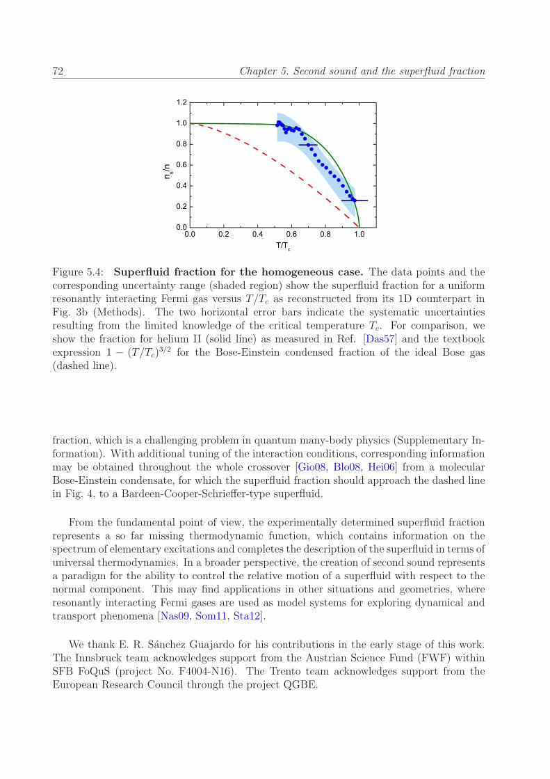
72 Chapter 5. Second sound and the superfluid fraction
Figure 5.4: Superfluid fraction for the homogeneous case. The data points and thecorresponding uncertainty range (shaded region) show the superfluid fraction for a uniformresonantly interacting Fermi gas versus T/Tc as reconstructed from its 1D counterpart inFig. 3b (Methods). The two horizontal error bars indicate the systematic uncertaintiesresulting from the limited knowledge of the critical temperature Tc. For comparison, weshow the fraction for helium II (solid line) as measured in Ref. [Das57] and the textbookexpression 1 − (T/Tc)
3/2 for the Bose-Einstein condensed fraction of the ideal Bose gas(dashed line).
fraction, which is a challenging problem in quantum many-body physics (Supplementary In-formation). With additional tuning of the interaction conditions, corresponding informationmay be obtained throughout the whole crossover [Gio08, Blo08, Hei06] from a molecularBose-Einstein condensate, for which the superfluid fraction should approach the dashed linein Fig. 4, to a Bardeen-Cooper-Schrieffer-type superfluid.
From the fundamental point of view, the experimentally determined superfluid fractionrepresents a so far missing thermodynamic function, which contains information on thespectrum of elementary excitations and completes the description of the superfluid in terms ofuniversal thermodynamics. In a broader perspective, the creation of second sound representsa paradigm for the ability to control the relative motion of a superfluid with respect to thenormal component. This may find applications in other situations and geometries, whereresonantly interacting Fermi gases are used as model systems for exploring dynamical andtransport phenomena [Nas09, Som11, Sta12].
We thank E. R. Sanchez Guajardo for his contributions in the early stage of this work.The Innsbruck team acknowledges support from the Austrian Science Fund (FWF) withinSFB FoQuS (project No. F4004-N16). The Trento team acknowledges support from theEuropean Research Council through the project QGBE.
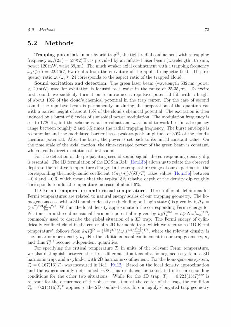
5.2. Methods 73
5.2 Methods
Trapping potential. In our hybrid trap31, the tight radial confinement with a trappingfrequency ωr/(2π) = 539(2)Hz is provided by an infrared laser beam (wavelength 1075 nm,power 120mW, waist 39µm). The much weaker axial confinement with a trapping frequencyωz/(2π) = 22.46(7)Hz results from the curvature of the applied magnetic field. The fre-quency ratio ωr/ωz ≈ 24 corresponds to the aspect ratio of the trapped cloud.
Sound excitation and detection. The green laser beam (wavelength 532 nm, power< 20mW) used for excitation is focused to a waist in the range of 25-35µm. To excitefirst sound, we suddenly turn it on to introduce a repulsive potential hill with a heightof about 10% of the cloud’s chemical potential in the trap center. For the case of secondsound, the repulsive beam is permanently on during the preparation of the quantum gaswith a barrier height of about 15% of the cloud’s chemical potential. The excitation is theninduced by a burst of 8 cycles of sinusoidal power modulation. The modulation frequency isset to 1720Hz, but the scheme is rather robust and was found to work best in a frequencyrange between roughly 2 and 3.5 times the radial trapping frequency. The burst envelope isrectangular and the modulated barrier has a peak-to-peak amplitude of 30% of the cloud’schemical potential. After the burst, the power is set back to its initial constant value. Onthe time scale of the axial motion, the time-averaged power of the green beam is constant,which avoids direct excitation of first sound.
For the detection of the propagating second-sound signal, the corresponding density dipis essential. The 1D formulation of the EOS in Ref. [Hou13b] allows us to relate the observeddepth to the relative temperature change. In the temperature range of our experiments, thecorresponding thermodynamic coefficient (δn1/n1)/(δT/T ) takes values [Hou13b] between−0.4 and −0.6, which means that the typical 3% relative depth of the density dip roughlycorresponds to a local temperature increase of about 6%.
1D Fermi temperature and critical temperature. Three different definitions forFermi temperatures are related to natural energy scales of our trapping geometry. The ho-mogeneous case with a 3D number density n (including both spin states) is given by kBTF =(3π2)2/3 ~
2
2mn2/3. Within the local density approximation the corresponding Fermi energy for
N atoms in a three-dimensional harmonic potential is given by kBTtrapF = ~(3N ω2
rωz)1/3,
commonly used to describe the global situation of a 3D trap. The Fermi energy of cylin-drically confined cloud in the center of a 2D harmonic trap, which we refer to as ‘1D Fermi
temperature’, follows from kBT1DF = (15π
8)2/5(~ωr)
4/5(~2n2
1
2m)1/5, where the relevant density is
the linear number density n1. For the additional axial confinement in our trap geometry, n1
and thus T 1DF become z-dependent quantities.
For specifying the critical temperature Tc in units of the relevant Fermi temperature,we also distinguish between the three different situations of a homogeneous system, a 3Dharmonic trap, and a cylinder with 2D harmonic confinement. For the homogeneous system,Tc = 0.167(13)TF was measured in Ref. [Ku12]. Based on the local density approximationand the experimentally determined EOS, this result can be translated into correspondingconditions for the other two situations. While for the 3D trap, Tc = 0.223(15)T trap
F isrelevant for the occurrence of the phase transition at the center of the trap, the conditionTc = 0.214(16)T 1D
F applies to the 2D confined case. In our highly elongated trap geometry
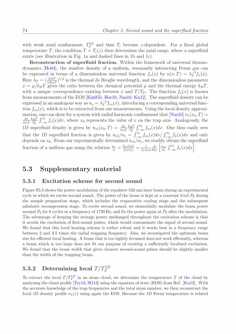
74 Chapter 5. Second sound and the superfluid fraction
with weak axial confinement, T 1DF and thus Tc become z-dependent. For a fixed global
temperature T , the condition T < Tc(z) then determines the axial range, where a superfluidexists (see illustration in Fig. 1a and dashed lines in 1b and 1c).
Reconstruction of superfluid fraction. Within the framework of universal thermo-dynamics [Ho04], the number density of a uniform, resonantly interacting Fermi gas canbe expressed in terms of a dimensionless universal function fn(x) by n(x, T ) = λ−3
T fn(x).
Here λT = ( 2π~2
mkBT)1/2 is the thermal de Broglie wavelength, and the dimensionless parameter
x = µ/kBT gives the ratio between the chemical potential µ and the thermal energy kBT ,with a unique correspondence existing between x and T/TF . The function fn(x) is knownfrom measurements of the EOS [Kin05b, Hor10, Nas10, Ku12]. The superfluid density can beexpressed in an analogous way as ns = λ−3
T fns(x), introducing a corresponding universal func-tion fns(x), which is to be extracted from our measurements. Using the local density approxi-mation, one can show for a system with radial harmonic confinement that [Nas10] n1(x0, T ) =2πmω2
r
kBTλ3
T
∫ x0
−∞fn(x)dx, where x0 represents the value of x on the trap axis. Analogously, the
1D superfluid density is given by ns1(x0, T ) = 2πmω2
r
kBTλ3
T
∫ x0
−∞fns(x)dx. One thus easily sees
that the 1D superfluid fraction is given by ns1/n1 =∫ x0
−∞fns(x)dx/
∫ x0
−∞fn(x)dx and only
depends on x0. From our experimentally determined ns1/n1, we readily obtain the superfluid
fraction of a uniform gas using the relation ns
n= fns(x0)
fn(x0)= 1
fn(x0)d
dx0
[
ns1
n1
∫ x0
−∞fn(x)dx
]
.
5.3 Supplementary material
5.3.1 Excitation scheme for second sound
Figure S5.5 shows the power modulation of the repulsive 532-nm laser beam during an experimentalcycle in which we excite second sound. The power of the beam is kept at a constant level P0 duringthe sample preparation stage, which includes the evaporative cooling stage and the subsequentadiabatic recompression stage. To excite second sound, we sinusoidally modulate the beam poweraround P0 for 8 cycles at a frequency of 1720Hz, and fix the power again at P0 after the modulation.The advantage of keeping the average power unchanged throughout the excitation scheme is thatit avoids the excitation of first-sound pulses, which would contaminate the signal of second sound.We found that this local heating scheme is rather robust and it works best in a frequency rangebetween 2 and 3.5 times the radial trapping frequency. Also, we investigated the optimum beamsize for efficient local heating. A beam that is too tightly focussed does not work efficiently, whereasa beam which is too large does not fit our purpose of creating a sufficiently localized excitation.We found that the beam width that gives clearest second-sound pulses should be slightly smallerthan the width of the trapping beam.
5.3.2 Determining local T/T 1DF
To extract the local T/T 1DF in an atom cloud, we determine the temperature T of the cloud by
analyzing the cloud profile [Tey13, SG13] using the equation of state (EOS) from Ref. [Ku12]. Withthe accurate knowledge of the trap frequencies and the total atom number, we then reconstruct thelocal 1D density profile n1(z) using again the EOS. Because the 1D Fermi temperature is related
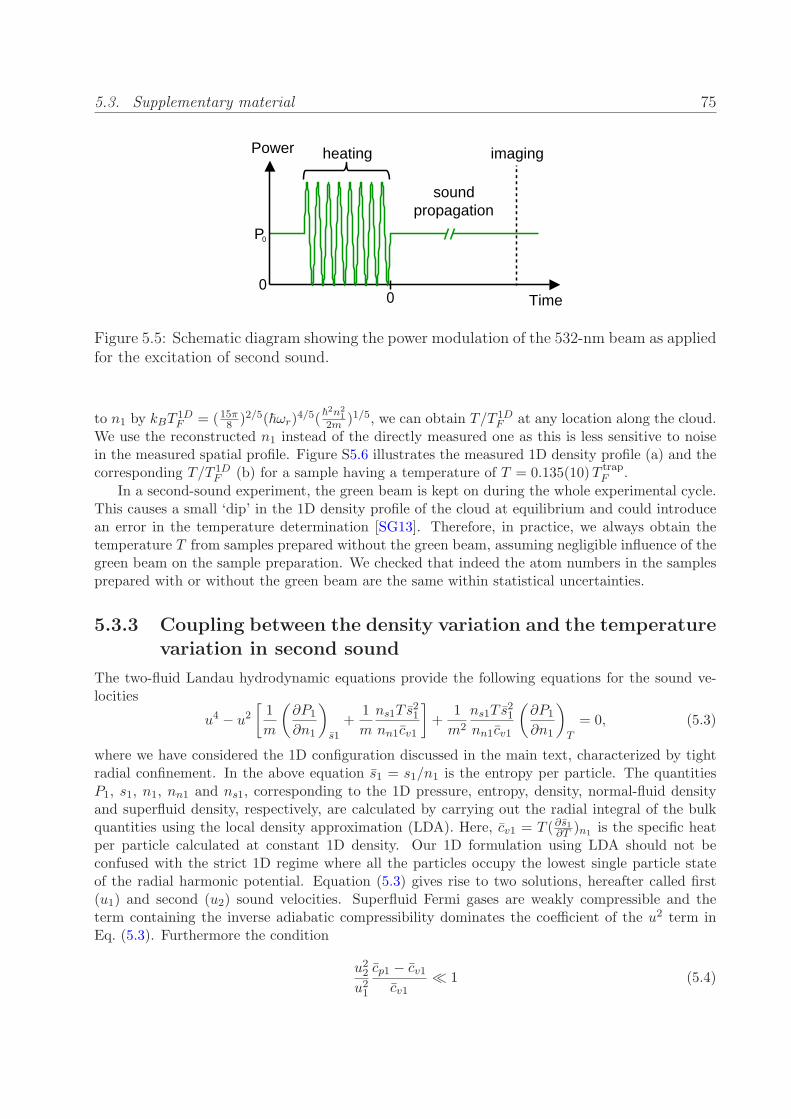
5.3. Supplementary material 75
imaging
Time00
Power heating
soundpropagation
P0
Figure 5.5: Schematic diagram showing the power modulation of the 532-nm beam as appliedfor the excitation of second sound.
to n1 by kBT1DF = (15π8 )2/5(~ωr)
4/5(~2n2
1
2m )1/5, we can obtain T/T 1DF at any location along the cloud.
We use the reconstructed n1 instead of the directly measured one as this is less sensitive to noisein the measured spatial profile. Figure S5.6 illustrates the measured 1D density profile (a) and thecorresponding T/T 1D
F (b) for a sample having a temperature of T = 0.135(10)T trapF .
In a second-sound experiment, the green beam is kept on during the whole experimental cycle.This causes a small ‘dip’ in the 1D density profile of the cloud at equilibrium and could introducean error in the temperature determination [SG13]. Therefore, in practice, we always obtain thetemperature T from samples prepared without the green beam, assuming negligible influence of thegreen beam on the sample preparation. We checked that indeed the atom numbers in the samplesprepared with or without the green beam are the same within statistical uncertainties.
5.3.3 Coupling between the density variation and the temperature
variation in second sound
The two-fluid Landau hydrodynamic equations provide the following equations for the sound ve-locities
u4 − u2[
1
m
(
∂P1
∂n1
)
s1
+1
m
ns1T s21
nn1cv1
]
+1
m2
ns1T s21
nn1cv1
(
∂P1
∂n1
)
T
= 0, (5.3)
where we have considered the 1D configuration discussed in the main text, characterized by tightradial confinement. In the above equation s1 = s1/n1 is the entropy per particle. The quantitiesP1, s1, n1, nn1 and ns1, corresponding to the 1D pressure, entropy, density, normal-fluid densityand superfluid density, respectively, are calculated by carrying out the radial integral of the bulkquantities using the local density approximation (LDA). Here, cv1 = T (∂s1∂T )n1
is the specific heatper particle calculated at constant 1D density. Our 1D formulation using LDA should not beconfused with the strict 1D regime where all the particles occupy the lowest single particle stateof the radial harmonic potential. Equation (5.3) gives rise to two solutions, hereafter called first(u1) and second (u2) sound velocities. Superfluid Fermi gases are weakly compressible and theterm containing the inverse adiabatic compressibility dominates the coefficient of the u2 term inEq. (5.3). Furthermore the condition
u22u21
cp1 − cv1cv1
≪ 1 (5.4)
76 Chapter 5. Second sound and the superfluid fraction
a
b
Figure 5.6: Position dependence of the measured linear number density n1 and the corre-sponding T/T 1D
F along the highly elongated atomic cloud. a, 1D density profile n1 averagedover eight samples prepared in an identical way. b, The corresponding local T/T 1D
F . Thehorizontal dashed line represents the critical temperature Tc = 0.214(16)T 1D
F for a cylindri-cally trapped gas with a harmonic radial confinement. The vertical dashed lines in botha and b indicate the boundaries within which a superfluid exists. The temperature of thesample is T = 0.135(10)T trap
F .
is always well satisfied. Under these conditions, the two solutions of Landau’s hydrodynamicequations take the simplified forms
u21 =1
m
(
∂P1
∂n1
)
s1
, (5.5)
and
u22 =1
m
ns1T s12
nn1cp1, (5.6)
where the derivative at constant s1 corresponds to an adiabatic transformation. At unitarityEqs. (5.5) and (5.6) reduce to Eqs. (1) and (2) in the main text after being normalized with the1D Fermi speed v1DF . Under the same condition (5.4) the first sound solution corresponds to anadiabatic wave, propagating at constant entropy per particle, while the second sound solution toan isobaric wave, propagating at constant pressure [Hou13b].
Because of the isobaric nature of the second sound mode the corresponding density variationsare related to the temperature variations by the equation
δn1/n1
δT/T=
T
n1
(
∂n1
∂T
)
P1
= −Tα1, (5.7)
5.3. Supplementary material 77
where α1 is the 1D thermal expansion coefficient. At unitarity α1 is directly related to the specificheats cp1 and cv1 by the simple relation Tα1 = (5/2)(cp1−cv1)/cv1 showing that, even for moderatelylarge values of α1, the condition (5.4) is well satisfied since u22 ≪ u21. We find that in the temperatureinterval related to our experiment the value of Tα1 is sufficiently large (between 0.4 and 0.6) toensure the visibility of the density signal associated with second sound.
5.3.4 Measurement uncertainties
The analysis and interpretation of our data is subject to various statistical and systematic uncer-tainties, which we here discuss in more detail. For a second-sound data set, as the one in Fig. 1cin the main text, we typically take a total number of 210 spatial profiles, recorded for 35 differentdelay times with 6 individual images for each delay time. Some shots (up to 3 per delay time)are rejected when the quality of the image is insufficient, e.g. because of interference fringes or un-usually large fluctuations in the atom number, and an average is taken over the remaining reliableprofiles. With an experimental cycle time of about 15 s, the total data acquisition time for a set likethe one in Fig. 1c is about 1 hour, which makes the experiment very sensitive to instabilities andexternal perturbations. To avoid slow drifts in the experiment causing any systematic behavior, wetake all 210 profiles in a fully random order. In addition, 6 profiles are recorded without the soundexcitation for determining the global temperature T .
Analyzing an individual set of measurements
The main source of uncertainties in our measured sound speeds and the derived superfluid fractionstems from the determination of the positions of the propagating pulses. The signal-to-noise ratio,i.e. the pulse amplitude versus background noise in the recorded density, is in general quite low, aswe apply only small perturbations to ensure linear behavior. The signal-to-noise ratio is roughly5 for the first-sound signal (after averaging) as presented in Fig. 1b in the main text. For thesecond-sound pulses (Fig. 1c) the signal-to-noise ratio is about 4 near the center of the cloud anddrops quickly to about 1 near the superfluid boundary. This explains the larger fluctuations in theposition of the second-sound pulse away from the cloud center as shown in Fig. 2a in the maintext. We carefully analyze the quality of the fit for each position data point and reject some of thepoints where the fit result is not reliable.
While determining the sound speeds we face the problem that even small noise in the positiondata results in substantial noise when the time derivative is taken. We therefore adopt two differentmethods, based on global and local fits to the position-versus-time data. Our first method is basedon a global fit to the whole set of position data points. Here we use a third-order polynomial,which we generally find to fit the data very well. The second-sound data set displayed in Fig. 2ahas in total 31 position data points (after the rejection of 4 unreliable points). Finally we takethe derivative of the fit curve to determine the sound speed as a function of delay time. Oursecond method is based on locally fitting a set of 9 adjacent points with a parabola. We define thelocal sound speed as the slope of this fit at the central (5th) point. The corresponding results arerepresented by the filled circles in Fig. 2b. This approach cannot give the local speeds at the first4 points and the last 4 points in the full data set. We thus extract the local speeds of the first 4data points simply from the derivative of the fit to the first 9 data points at the 1st, 2nd, 3rd, and4th positions. The same procedure is applied to the last 4 data points.
While the first method relies on the assumption of a global fit function and thus provides asmooth curve, the second one is a compromise between extracting local information, independentof a specific fit function, and the noise reduction from a fit to several points. In the first method,
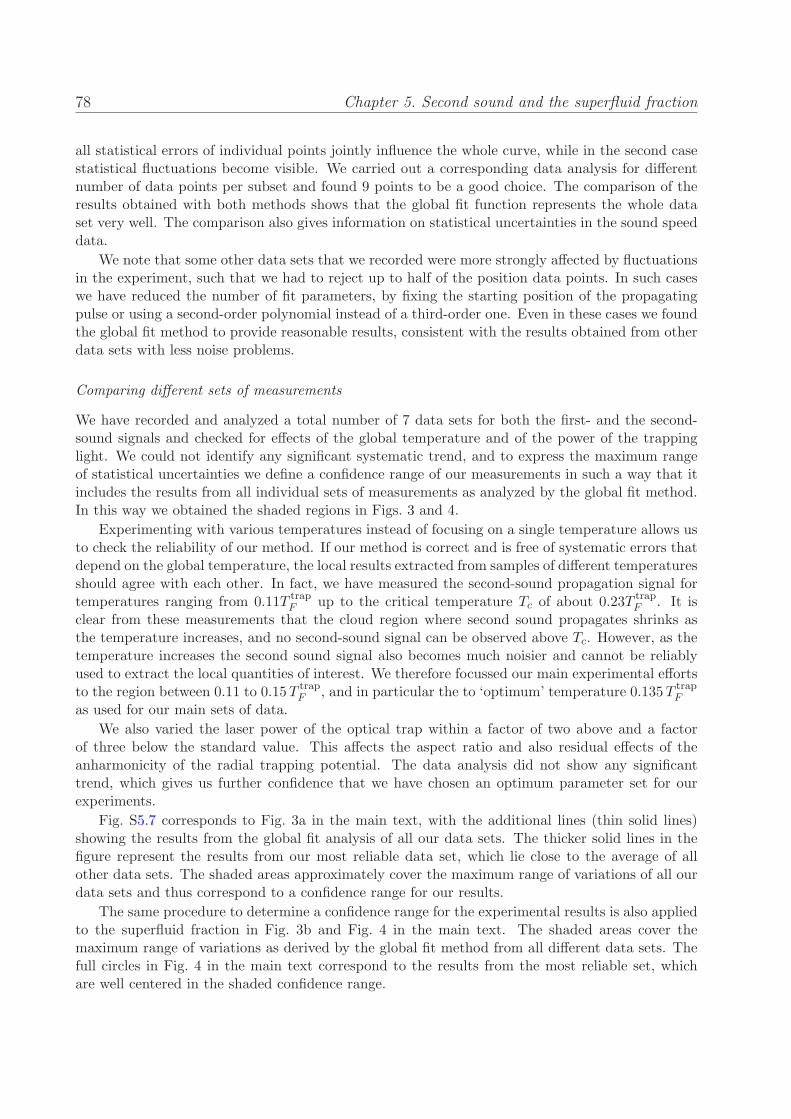
78 Chapter 5. Second sound and the superfluid fraction
all statistical errors of individual points jointly influence the whole curve, while in the second casestatistical fluctuations become visible. We carried out a corresponding data analysis for differentnumber of data points per subset and found 9 points to be a good choice. The comparison of theresults obtained with both methods shows that the global fit function represents the whole dataset very well. The comparison also gives information on statistical uncertainties in the sound speeddata.
We note that some other data sets that we recorded were more strongly affected by fluctuationsin the experiment, such that we had to reject up to half of the position data points. In such caseswe have reduced the number of fit parameters, by fixing the starting position of the propagatingpulse or using a second-order polynomial instead of a third-order one. Even in these cases we foundthe global fit method to provide reasonable results, consistent with the results obtained from otherdata sets with less noise problems.
Comparing different sets of measurements
We have recorded and analyzed a total number of 7 data sets for both the first- and the second-sound signals and checked for effects of the global temperature and of the power of the trappinglight. We could not identify any significant systematic trend, and to express the maximum rangeof statistical uncertainties we define a confidence range of our measurements in such a way that itincludes the results from all individual sets of measurements as analyzed by the global fit method.In this way we obtained the shaded regions in Figs. 3 and 4.
Experimenting with various temperatures instead of focusing on a single temperature allows usto check the reliability of our method. If our method is correct and is free of systematic errors thatdepend on the global temperature, the local results extracted from samples of different temperaturesshould agree with each other. In fact, we have measured the second-sound propagation signal fortemperatures ranging from 0.11T trap
F up to the critical temperature Tc of about 0.23T trapF . It is
clear from these measurements that the cloud region where second sound propagates shrinks asthe temperature increases, and no second-sound signal can be observed above Tc. However, as thetemperature increases the second sound signal also becomes much noisier and cannot be reliablyused to extract the local quantities of interest. We therefore focussed our main experimental effortsto the region between 0.11 to 0.15T trap
F , and in particular the to ‘optimum’ temperature 0.135T trapF
as used for our main sets of data.
We also varied the laser power of the optical trap within a factor of two above and a factorof three below the standard value. This affects the aspect ratio and also residual effects of theanharmonicity of the radial trapping potential. The data analysis did not show any significanttrend, which gives us further confidence that we have chosen an optimum parameter set for ourexperiments.
Fig. S5.7 corresponds to Fig. 3a in the main text, with the additional lines (thin solid lines)showing the results from the global fit analysis of all our data sets. The thicker solid lines in thefigure represent the results from our most reliable data set, which lie close to the average of allother data sets. The shaded areas approximately cover the maximum range of variations of all ourdata sets and thus correspond to a confidence range for our results.
The same procedure to determine a confidence range for the experimental results is also appliedto the superfluid fraction in Fig. 3b and Fig. 4 in the main text. The shaded areas cover themaximum range of variations as derived by the global fit method from all different data sets. Thefull circles in Fig. 4 in the main text correspond to the results from the most reliable set, whichare well centered in the shaded confidence range.
5.3. Supplementary material 79
Figure 5.7: Normalized speeds for the first and second sound obtained from different datasets. The thick solid lines and full circles are identical to those shown in Fig. 3a in themain text. The thick solid lines represent the global-fit results of the most reliable first- andsecond-sound data sets whose values also lie close to the ‘average’ of other data sets. Thethinner solid lines represent the global-fit results from all other data sets. The shaded areasapproximately cover the maximum range of variations of all fits.
Systematic uncertainties
Various possible sources of systematic errors are present. We can determine the number of atomswithin a calibration error of 20%, which leads to an uncertainty in the 1D Fermi temperatures ofless than 8% and in the Fermi speeds of less than 4%. The uncertainty arising from the calibrationof the imaging scale is less than 2% and thus negligibly small. The uncertainty in the determinationof the global temperature is about 10% near the superfluid phase transition and about 15% for thelowest temperatures investigated, see Ref. [Tey13]. Individual data sets as the ones presented inFig. 1b and 1c are analyzed under the assumption of a constant temperature. Therefore any kindof uncertainty in the determination of this temperature appears as a systematic effect in the wholeset.
The interpretation of our results relies on knowledge of the equation of state (EOS); here weuse the most recent measurements [Ku12] published by the MIT group. The EOS is used fordetermining the global temperatures from the spatial profiles, and provides the necessary thermo-dynamic functions to derive the superfluid fraction. The noise in the EOS data is so small thatstatistical uncertainties in our analysis remain well below other noise sources. Small systematicuncertainties may be present, which are very difficult to be quantified. Since the MIT data werecarefully benchmarked with certain limiting cases, like the ideal non-interacting Fermi gas, and adetailed discussion in comparison with previous experimental results and theoretical approacheswas provided, we are very confident that systematic uncertainties in the EOS are so small thatthey do not affect our data in a significant way.
A further source of an uncertainty may result from limitations to the validity of the 1D hydro-dynamic approach in our elongated trap. However, our previous investigation of the temperaturedependence of higher-nodal first-sound collective modes in Ref. [Tey13] shows excellent agreement
80 Chapter 5. Second sound and the superfluid fraction
of the observed and calculated mode frequencies on the level of a few 10−3. Moreover, in thepresent experiments we get essentially perfect agreement between observed and calculated first-sound velocities. We have no reason to believe that second sound is more sensitive to a breakdownof the 1D hydrodynamic approach to solve Landau’s two-fluid equations than first sound. Also thedata sets that we took with smaller aspect ratios do not reveal any significant trend. Thereforewe are confident that our 1D hydrodynamic approach is an excellent approximation to the realexperimental situation and does not provide significant systematic uncertainties.
We finally note that we have also checked in how far the use of Eq. (5.6), rather than using theexact solution of Eq. (5.3), affects the determination of the superfluid fraction from the measuredsecond-sound speed. Deviations stay below one percent and are thus negligible as compared to theother uncertainties.
5.3.5 Available theoretical models for the superfluid fraction ns/n
Several authors have already provided theoretical predictions for the temperature dependence of thesuperfluid fraction of the uniform Fermi gas at unitarity. A comprehensive discussion is contained inthe publication [Tay08] by Taylor et al. However, it is not natural to compare these predictions withthe experimental findings reported in our present work. The available calculations in fact predictvalues of the critical temperature which are in general significantly higher than the experimentalvalue of 0.167(13) TF (Ref. [Ku12]). Therefore, the comparison in the temperature range relevantto our experiment (0.09 < T/TF < 0.16), where the fraction ns/n significantly deviates from unity,is not particularly useful. Theoretical predictions in the lower temperature region, correspondingto T/TF < 0.09 and accounting for the effects of fermionic excitations in addition to the leadingphonon contribution, have been also reported [And03, Sal10], but we have no data for comparisonin this temperature range. On the other hand, the most reliable quantum many-body calculationsproviding accurate values for the critical temperature of the superfluid transition [Bur06, Hau07,Gou10] have not yet provided predictions for the temperature dependence of the superfluid fraction.
Bibliography
[Ada94] C. S. Adams, M. Sigel, and J. Mlynek, Atom optics, Phys. Rep. 240, 143 (1994).
[All38] J. F. Allen and A. D. Misener, Flow Phenomena in Liquid Helium II, Nature 142, 643(1938).
[Alt07a] A. Altmeyer, Collective oscillations of an ultracold quantum gas in the BEC-BCScrossover regime, Ph.D. thesis, University of Innsbruck (2007).
[Alt07b] A. Altmeyer, S. Riedl, C. Kohstall, M. J. Wright, R. Geursen, M. Bartenstein, C. Chin,J. Hecker Denschlag, and R. Grimm, Precision Measurements of Collective Oscillationsin the BEC-BCS Crossover, Phys. Rev. Lett. 98, 040401 (2007).
[Alt07c] A. Altmeyer, S. Riedl, M. J. Wright, C. Kohstall, J. Hecker Denschlag, and R. Grimm,Dynamics of a strongly interacting Fermi gas: The radial quadrupole mode, Phys. Rev.A 76, 033610 (2007).
[And95] M. H. Anderson, J. R. Ensher, M. R. Matthews, C. E. Wieman, and E. A. Cornell,Observation of Bose-Einstein condensation in dilute atomic vapor, Science 269, 198(1995).
[And97a] M. R. Andrews, D. M. Kurn, H.-J. Miesner, D. S. Durfee, C. G. Townsend, S. Inouye,and W. Ketterle, Propagation of Sound in a Bose-Einstein Condensate, Phys. Rev. Lett.79, 553 (1997).
[And97b] M. R. Andrews, C. G. Townsend, H.-J. Miesner, D. S. Durfee, D. M. Kurn, and W. Ket-terle, Observation of interference between two Bose condensates, Science 275, 637 (1997).
[And03] N. Andrenacci, P. Pieri, and G. C. Strinati, Evolution from BCS superconductivity toBose-Einstein condensation: Current correlation function in the broken-symmetry phase,Phys. Rev. B 68, 144507 (2003).
[Ara09] E. Arahata and T. Nikuni, Propagation of second sound in a superfluid Fermi gas in theunitary limit, Phys. Rev. A 80, 043613 (2009).
[Arn99] M. Arndt, O. Nairz, J. Vos-Andreae, C. Keller, G. van der Zouw, and A. Zeilinger,Wave-particle duality of C-60 molecules, Nature 401, 680 (1999).
[Atk59] K. R. Atkins, Liquid helium, Cambridge University Press, Cambridge (1959).
[Ban00] Y. B. Band, M. Trippenbach, J. P. Burke, and P. S. Julienne, Elastic Scattering Lossof Atoms from Colliding Bose-Einstein Condensate Wave Packets, Phys. Rev. Lett. 84,5462 (2000).
81
82 Bibliography
[Ban01] Y. B. Band, J. P. Burke, A. Simoni, and P. S. Julienne, Suppression of elastic scatteringloss for slowly colliding Bose-Einstein condensates, Phys. Rev. A 64, 023607 (2001).
[Bar04a] M. Bartenstein, A. Altmeyer, S. Riedl, S. Jochim, C. Chin, J. Hecker Denschlag, andR. Grimm, Collective Excitations of a Degenerate Gas at the BEC-BCS Crossover, Phys.Rev. Lett. 92, 203201 (2004).
[Bar04b] M. Bartenstein, A. Altmeyer, S. Riedl, S. Jochim, C. Chin, J. Hecker Denschlag, andR. Grimm, Crossover from a Molecular Bose-Einstein Condensate to a Degenerate FermiGas, Phys. Rev. Lett. 92, 120401 (2004).
[Bar05a] M. Bartenstein, From Molecules to Cooper Pairs: Experiments in the BEC-BCSCrossover, Ph.D. thesis, Innsbruck University (2005).
[Bar05b] M. Bartenstein, A. Altmeyer, S. Riedl, R. Geursen, S. Jochim, C. Chin, J. Hecker Den-schlag, R. Grimm, A. Simoni, E. Tiesinga, C. J. Williams, and P. S. Julienne, Precisedetermination of 6Li cold collision parameters by radio-frequency spectroscopy on weaklybound molecules, Phys. Rev. Lett. 94, 103201 (2005).
[Bar13] C. E. Bardyn, M. A. Baranov, C. V. Kraus, E. Rico, A. Imamoglu, P. Zoller, and S. Diehl,Topology by dissipation, arXiv:1302.5135 (2013).
[Bed88] J. G. Bednorz and K. A. Muller, Perovskite-Type Oxides - the New Approach to High-Tc Superconductivity. Nobel Lecture, Angewandte Chemie International Edition 27, 735(1988).
[Ber10] G. Bertaina, L. Pitaevskii, and S. Stringari, First and Second Sound in CylindricallyTrapped Gases, Phys. Rev. Lett. 105, 150402 (2010).
[Blo08] I. Bloch, J. Dalibard, and W. Zwerger, Many-body physics with ultracold gases, Rev.Mod. Phys. 80, 885 (2008).
[Blo12] I. Bloch, J. Dalibard, and S. Nascimbene, Quantum simulations with ultracold quantumgases, Nature Phys. 8, 267 (2012).
[Bon04] K. Bongs and K. Sengstock, Physics with coherent matter waves, Rep. Prog. Phys. 67,907 (2004).
[Bra95] C. C. Bradley, C. A. Sackett, J. J. Tollett, and R. G. Hulet, Evidence of Bose-Einsteincondensation in an atomic gas with attractive interactions, Phys. Rev. Lett. 75, 1687(1995).
[Bro23] L. de Broglie, Waves and quanta, Nature 112, 540 (1923).
[Bug04] C. Buggle, J. Leonard, W. von Klitzing, and J. T. M. Walraven, Interferometric De-termination of the s and d-Wave Scattering Amplitudes in 87Rb, Phys. Rev. Lett. 93,173202 (2004).
[Bul05] A. Bulgac, Specific Heat of a Fermionic Atomic Cloud in the Unitary Regime, Phys. Rev.Lett. 95, 140403 (2005).
[Bur06] E. Burovski, N. Prokof’ev, B. Svistunov, and M. Troyer, Critical Temperature and Ther-modynamics of Attractive Fermions at Unitarity, Phys. Rev. Lett. 96, 160402 (2006).

Bibliography 83
[Cao11a] C. Cao, E. Elliott, J. Joseph, J. Petricka, T. Schafer, and J. E. Thomas, UniversalQuantum Viscosity in a Unitary Fermi Gas, Science 331, 58 (2011).
[Cao11b] C. Cao, E. Elliott, H. Wu, and J. E. Thomas, Searching for perfect fluids: quantumviscosity in a universal Fermi gas, New J. Phys. 13, 075007 (2011).
[Cap06] P. Capuzzi, P. Vignolo, F. Federici, and M. P. Tosi, Sound propagation in elongatedsuperfluid fermionic clouds, Phys. Rev. A 73, 021603 (2006).
[Car02] E. W. Carlson, V. J. Emery, S. A. Kivelson, and D. Orgad, Concepts in High TemperatureSuperconductivity, arXiv:cond-mat/0206217 (2002).
[Cas97] Y. Castin and J. Dalibard, Relative phase of two Bose-Einstein condensates, Phys. Rev.A 55, 4330 (1997).
[Ced07] L. S. Cederbaum, A. I. Streltsov, Y. B. Band, and O. E. Alon, Interferences in theDensity of Two Bose-Einstein Condensates Consisting of Identical or Different Atoms,Phys. Rev. Lett. 98, 110405 (2007).
[Che05] Q. Chen, J. Stajic, S. Tan, and K. Levin, BCS-BEC Crossover: From High TemperatureSuperconductors to Ultracold Superfluids, Phys. Rep. 412, 1 (2005).
[Che09] Q. Chen and K. Levin, Momentum Resolved Radio Frequency Spectroscopy in TrappedFermi Gases, Phys. Rev. Lett. 102, 190402 (2009).
[Che10] F. Chevy and C. Mora, Ultra-cold polarized Fermi gases, Rep. Prog. Phys. 73, 112401(2010).
[Chi00] A. P. Chikkatur, A. Gorlitz, D. M. Stamper-Kurn, S. Inouye, S. Gupta, and W. Ketterle,Suppression and Enhancement of Impurity Scattering in a Bose-Einstein Condensate,Phys. Rev. Lett. 85, 483 (2000).
[Chi04] C. Chin, M. Bartenstein, A. Altmeyer, S. Riedl, S. Jochim, J. Hecker Denschlag, andR. Grimm, Observation of the Pairing Gap in a Strongly Interacting Fermi Gas, Science305, 1128 (2004).
[Chi10] C. Chin, R. Grimm, P. S. Julienne, and E. Tiesinga, Feshbach resonances in ultracoldgases, Rev. Mod. Phys. 82, 1225 (2010).
[Cho12] L. Chomaz, L. Corman, T. Yefsah, R. Desbuquois, and J. Dalibard, Absorption imagingof a quasi-two-dimensional gas: a multiple scattering analysis, New J. Phys. 14, 055001(2012).
[Chu98] S. Chu, Nobel Lecture: The manipulation of neutral particles, Rev. Mod. Phys. 70, 685(1998).
[Com06] R. Combescot, S. Giorgini, and S. Stringari, Molecular signatures in the structure factorof an interacting Fermi gas, EPL (Europhysics Letters) 75, 695 (2006).
[Cou98] P. Courteille, R. S. Freeland, D. J. Heinzen, F. A. van Abeelen, and B. J. Verhaar,Observation of a Feshbach Resonance in Cold Atom Scattering, Phys. Rev. Lett. 81, 69(1998).
84 Bibliography
[Cro09] A. D. Cronin, J. Schmiedmayer, and D. E. Pritchard, Optics and interferometry withatoms and molecules, Rev. Mod. Phys. 81, 1051 (2009).
[CT98] C. N. Cohen-Tannoudji, Nobel Lecture: Manipulating atoms with photons, Rev. Mod.Phys. 70, 707 (1998).
[Cub03] J. Cubizolles, T. Bourdel, S. J. J. M. F. Kokkelmans, G. V. Shlyapnikov, and C. Salomon,Production of Long-Lived Ultracold Li2 Molecules from a Fermi Gas, Phys. Rev. Lett.91, 240401 (2003).
[Dal99] F. Dalfovo, S. Giorgini, L. P. Pitaevskii, and S. Stringari, Theory of Bose-Einstein con-densation in trapped gases, Rev. Mod. Phys. 71, 463 (1999).
[Das57] J. G. Dash and R. D. Taylor, Hydrodynamics of Oscillating Disks in Viscous Fluids:Density and Viscosity of Normal Fluid in Pure He4 from 1.2◦K to the Lambda Point,Phys. Rev. 105, 7 (1957).
[Dav27] C. J. Davisson and L. H. Germer, The scattering of electrons by a single crystal of nickel,Nature 119, 558560 (1927).
[Dav95] K. B. Davis, M. O. Mewes, M. R. Andrews, N. J. van Druten, D. S. Durfee, D. M. Kurn,and W. Ketterle, Bose-Einstein condensation in a gas of sodium atoms, Phys. Rev. Lett.75, 3969 (1995).
[DeM99] B. DeMarco and D. S. Jin, Onset of Fermi Degeneracy in a Trapped Atomic Gas, Science285, 1703 (1999).
[DeS10] B. J. DeSalvo, M. Yan, P. G. Mickelson, Y. N. Martinez de Escobar, and T. C. Killian,Degenerate Fermi Gas of 87Sr, Phys. Rev. Lett. 105, 030402 (2010).
[DG66] P. De Gennes, Superconductivity Of Metals And Alloys, W.A. Benjamin, Inc., New York- Amsterdam (1966).
[Don01] E. A. Donley, N. R. Clausen, S. L. Cornish, J. L. Roberts, E. A. Cornell, and C. E.Wieman, Dynamics of Collapsing and Exploding Bose-Einstein Condensates, Nature412, 295 (2001).
[DS05] L. De Sarlo, L. Fallani, J. E. Lye, M. Modugno, R. Saers, C. Fort, and M. Inguscio,Unstable regimes for a Bose-Einstein condensate in an optical lattice, Phys. Rev. A 72,013603 (2005).
[Est30] I. Estermann and O. Stern, Beugung von Molekularstrahlen, Z. Phys. 61, 95 (1930).
[Fan61] U. Fano, Effects of configuration interaction on intensities and phase shifts, Phys. Rev.124, 1866 (1961).
[Fer08] F. Ferlaino, S. Knoop, M. Mark, M. Berninger, H. Schobel, H.-C. Nagerl, and R. Grimm,Collisions between tunable halo dimers: Exploring an elementary four-body process withidentical bosons, Phys. Rev. Lett. 101, no. 2, 023201 (2008).
[Fer11] F. Ferlaino, A. Zenesini, M. Berninger, B. Huang, H.-C. Nagerl, and R. Grimm, EfimovResonances in Ultracold Quantum Gases, Few-Body Systems 51, 113 (2011).
Bibliography 85
[Fes58] H. Feshbach, United theory of nuclear reations, Ann. Phys. 5, 357 (1958).
[Fes62] H. Feshbach, United theory of nuclear reations II, Ann. Phys. 19, 287 (1962).
[Fuk07a] T. Fukuhara, Y. Takasu, M. Kumakura, and Y. Takahashi, Degenerate Fermi Gases ofYtterbium, Phys. Rev. Lett. 98, 030401 (2007).
[Fuk07b] T. Fukuhara, Y. Takasu, S. Sugawa, and Y. Takahashi, Quantum Degenerate FermiGases of Ytterbium Atoms, J. Low Temp. Phys. 148, 441 (2007).
[Fuk07c] N. Fukushima, Y. Ohashi, E. Taylor, and A. Griffin, Superfluid density and condensatefraction in the BCS-BEC crossover regime at finite temperatures, Phys. Rev. A 75,033609 (2007).
[Gae10] J. P. Gaebler, J. T. Stewart, T. E. Drake, D. S. Jin, A. Perali, P. Pieri, and G. C.Strinati, Observation of pseudogap behaviour in a strongly interacting Fermi gas, NaturePhys. 6, 569 (2010).
[Gal13] V. Galitski and I. B. Spielman, Spin-orbit coupling in quantum gases, Nature 494, 49(2013).
[Gar00] C. W. Gardiner, J. Ye, H. C. Nagerl, and H. J. Kimble, Evaluation of heating effects onatoms trapped in an optical trap, Phys. Rev. A 61, 045801 (2000).
[Geh98] M. E. Gehm, K. M. O’Hara, T. A. Savard, and J. E. Thomas, Dynamics of noise-inducedheating in atom traps, Phys. Rev. A 58, 3914 (1998).
[Ger11] S. Gerlich, S. Eibenberger, M. Tomandl, S. Nimmrichter, K. Hornberger, P. J. Fagan,J. Tuxen, M. Mayor, and M. Arndt, Quantum interference of large organic molecules,Nat. Commun. 2, 263 (2011).
[Gio08] S. Giorgini, L. P. Pitaevskii, and S. Stringari, Theory of ultracold atomic Fermi gases,Rev. Mod. Phys. 80, 1215 (2008).
[Gly00] H. R. Glyde, R. T. Azuah, and W. G. Stirling, Condensate, momentum distribution, andfinal-state effects in liquid 4He, Phys. Rev. B 62, 14337 (2000).
[Gou10] O. Goulko and M. Wingate, Thermodynamics of balanced and slightly spin-imbalancedFermi gases at unitarity, Phys. Rev. A 82, 053621 (2010).
[Gra02] S. R. Granade, M. E. Gehm, K. M. O’Hara, and J. E. Thomas, All-Optical Productionof a Degenerate Fermi Gas, Phys. Rev. Lett. 88, 120405 (2002).
[Gre03] M. Greiner, C. A. Regal, and D. S. Jin, Emergence of a Molecular Bose-Einstein Con-densate from a Fermi Gas, Nature 426, 537 (2003).
[Gre05] M. Greiner, C. A. Regal, and D. S. Jin, Probing the Excitation Spectrum of a Fermi Gasin the BCS-BEC Crossover Regime, Phys. Rev. Lett. 94, 070403 (2005).
[Gri88] R. Grimm and J. Mlynek, Observation of Light-Pressure-Induced Dispersion in Yb Vapor,Phys. Rev. Lett. 61, 2308 (1988).
86 Bibliography
[Gri97] A. Griffin and E. Zaremba, First and second sound in a uniform Bose gas, Phys. Rev.A 56, 4839 (1997).
[Gri00] R. Grimm, M. Weidemuller, and Y. B. Ovchinnikov, Optical dipole traps for neutralatoms, Adv. At. Mol. Opt. Phys. 42, 95 (2000).
[Gup03] S. Gupta, Z. Hadzibabic, M. W. Zwierlein, C. A. Stan, K. Dieckmann, C. H. Schunck,E. G. M. van Kempen, B. J. Verhaar, and W. Ketterle, Radio-Frequency Spectroscopy ofUltracold Fermions, Science 300, 1723 (2003).
[Had02] Z. Hadzibabic, C. A. Stan, K. Dieckmann, S. Gupta, M. W. Zwierlein, A. Gorlitz, andW. Ketterle, Two-Species Mixture of Quantum Degenerate Bose and Fermi Gases, Phys.Rev. Lett. 88, 160401 (2002).
[Had06] Z. Hadzibabic, P. Krger, M. Cheneau, B. Battelier, and J. Dalibard, Berezinskii-Kosterlitz-Thouless crossover in a trapped atomic gas, Nature 441, 1118 (2006).
[Hau07] R. Haussmann, W. Rantner, S. Cerrito, and W. Zwerger, Thermodynamics of the BCS-BEC crossover, Phys. Rev. A 75, 023610 (2007).
[Hau08] R. Haussmann and W. Zwerger, Thermodynamics of a trapped unitary Fermi gas, Phys.Rev. A 78, 063602 (2008).
[He07] Y. He, Q. Chen, C.-C. Chien, and K. Levin, First- and second-sound-like modes at finitetemperature in trapped Fermi gases from BCS to BEC, Phys. Rev. A 76, 051602 (2007).
[Hei04] H. Heiselberg, Collective Modes of Trapped Gases at the BEC-BCS Crossover, Phys.Rev. Lett. 93, 040402 (2004).
[Hei06] H. Heiselberg, Sound modes at the BCS-BEC crossover, Phys. Rev. A 73, 013607 (2006).
[Hem81] P. R. Hemmer, F. Y. Wu, and S. Ezekiel, Influence of atomic recoil on power broadenedlineshapes in 2-level atoms, Opt. Commun. 38, 105 (1981).
[Hen03] G. Hendel, Atom - Atom Wechselwirkung in einem ultrakalten, fermionischen Gas,Diploma thesis, University of Innsbruck (2003).
[Ho04] T.-L. Ho, Universal Thermodynamics of Degenerate Quantum Gases in the UnitarityLimit, Phys. Rev. Lett. 92, 090402 (2004).
[Ho10] T.-L. Ho and Q. Zhou, Obtaining the phase diagram and thermodynamic quantities ofbulk systems from the densities of trapped gases, Nature Phys. 6, 0131 (2010).
[Hof07] S. Hofferberth, I. Lesanovsky, B. Fischer, T. Schumm, and J. Schmiedmayer, Non-equilibrium coherence dynamics in one-dimensional Bose gases, Nature 449, 324 (2007).
[Hor10] M. Horikoshi, S. Nakajima, M. Ueda, and T. Mukaiyama, Measurement of universalthermodynamic functions for a unitary Fermi gas, Science 327, 442 (2010).
[Hou13a] Y.-H. Hou, L. Pitaevskii, and S. Stringari, Scaling solutions of the two-fluid hydrodynamicequations in a harmonically trapped gas at unitarity, Phys. Rev. A 87, 033620 (2013).

Bibliography 87
[Hou13b] Y.-H. Hou, L. P. Pitaevskii, and S. Stringari, First and second sound in a highly elongatedFermi gas at unitarity, arXiv:1301.4419 (2013).
[Hu07] H. Hu, P. D. Drummond, and X.-J. Liu, Universal thermodynamics of strongly interactingFermi gases, Nature Phys. 3, 469 (2007).
[Hu10] H. Hu, E. Taylor, X.-J. Liu, S. Stringari, and A. Griffin, Second sound and the densityresponse function in uniform superfluid atomic gases, New J. Phys. 12, 043040 (2010).
[Ing08] M. Inguscio, W. Ketterle, and C. Salomon (Eds.), Ultra-cold Fermi Gases, IOS Press,Amsterdam (2008), Proceedings of the International School of Physics “Enrico Fermi”,Course CLXIV, Varenna, 20-30 June 2006.
[Ino98] S. Inouye, M. R. Andrews, J. Stenger, H.-J. Miesner, D. M. Stamper-Kurn, and W. Ket-terle, Observation of Feshbach resonances in a Bose-Einstein condensate, Nature 392,151 (1998).
[Ino01] S. Inouye, S. Gupta, T. Rosenband, A. P. Chikkatur, A. Gorlitz, T. L. Gustavson, A. E.Leanhardt, D. E. Pritchard, and W. Ketterle, Observation of Vortex Phase Singularitiesin Bose-Einstein Condensates, Phys. Rev. Lett. 87, 080402 (2001).
[Joc03a] S. Jochim, M. Bartenstein, A. Altmeyer, G. Hendl, C. Chin, J. Hecker Denschlag, andR. Grimm, Pure Gas of Optically Trapped Molecules Created from Fermionic Atoms,Phys. Rev. Lett 91, 240402 (2003).
[Joc03b] S. Jochim, M. Bartenstein, A. Altmeyer, G. Hendl, S. Riedl, C. Chin, J. Hecker Den-schlag, and R. Grimm, Bose-Einstein Condensation of Molecules, Science 302, 2101(2003).
[Joc04] S. Jochim, Bose-Einstein Condensation of Molecules, Ph.D. thesis, Innsbruck University(2004).
[Jos07] J. Joseph, B. Clancy, L. Luo, J. Kinast, A. Turlapov, and J. E. Thomas, Measurement ofSound Velocity in a Fermi Gas near a Feshbach Resonance, Phys. Rev. Lett. 98, 170401(2007).
[Jos11] J. A. Joseph, J. E. Thomas, M. Kulkarni, and A. G. Abanov, Observation of ShockWaves in a Strongly Interacting Fermi Gas, Phys. Rev. Lett. 106, 150401 (2011).
[Kap38] P. Kapitza, Viscosity of liquid helium below the λ-point, Nature 141, 74 (1938).
[Kha65] I. M. Khalatnikov, An Introduction to the Theory of Superfluidity, Benjamin, New York(1965).
[Kin04a] J. Kinast, S. L. Hemmer, M. E. Gehm, A. Turlapov, and J. E. Thomas, Evidence forSuperfluidity in a Resonantly Interacting Fermi Gas, Phys. Rev. Lett. 92, 150402 (2004).
[Kin04b] J. Kinast, A. Turlapov, and J. E. Thomas, Breakdown of Hydrodynamics in the RadialBreathing Mode of a Strongly Interacting Fermi Gas, Phys. Rev. A 70, 051401(R) (2004).
[Kin05a] J. Kinast, A. Turlapov, and J. E. Thomas, Damping of a Unitary Fermi Gas, Phys. Rev.Lett. 94, 170404 (2005).
88 Bibliography
[Kin05b] J. Kinast, A. Turlapov, J. E. Thomas, Q. Chen, J. Stajic, and K. Levin, Heat Capacityof a Strongly Interacting Fermi Gas, Science 307, 1296 (2005).
[Koh06] T. Kohler, K. Goral, and P. S. Julienne, Production of cold molecules via magneticallytunable Feshbach resonances, Rev. Mod. Phys. 78, 1131 (2006).
[Koh07] C. Kohstall, A New Toolbox for Experiments with Ultracold 6Li, Diploma thesis, Univer-sity of Innsbruck (2007).
[Ku12] M. J. H. Ku, A. T. Sommer, L. W. Cheuk, and M. W. Zwierlein, Revealing the SuperfluidLambda Transition in the Universal Thermodynamics of a Unitary Fermi Gas, Science335, 563 (2012).
[Kuh11] E. D. Kuhnle, S. Hoinka, H. Hu, P. Dyke, P. Hannaford, and C. J. Vale, Studies of theuniversal contact in a strongly interacting Fermi gas using Bragg spectroscopy, New J.Phys. 13, 055010 (2011).
[Lan41] L. Landau, The theory of superfluidity of helium II, J. Phys. (Moscow) 5, 71 (1941).
[Lan47] L. Landau, On the theory of superfluidity of helium II, J. Phys. (Moscow) 11, 91 (1947).
[Lan77] L. D. Landau and E. M. Lifshitz, Quantum Mechanics, vol. 3 (Course of theoreticalphysics), Butterworth-Heinemann, Oxford (1977).
[Lan80a] L. D. Landau and E. M. Lifshitz, Statistical physics part 1, vol. 5 (Course of theoreticalphysics), Pergamon Press, Oxford (1980).
[Lan80b] L. D. Landau and E. M. Lifshitz, Statistical physics part 2, vol. 9 (Course of theoreticalphysics), Pergamon Press, Oxford (1980).
[Lan93] L. D. Landau and E. M. Lifshitz, Mechanics, vol. 1 (Course of theoretical physics),Butterworth-Heinemann, Oxford (1993).
[Lee57] T. D. Lee, K. Huang, and C. N. Yang, Eigenvalues and Eigenfunctions of a Bose Systemof Hard Spheres and its Low-Temperature Properties, Phys. Rev. 106, 1135 (1957).
[Leg80] A. J. Leggett, in A. Pekalski and R. Przystawa (Eds.), Modern Trends in the Theory ofCondensed Matter, volume 115 of Lecture Notes in Physics, 13, Springer Verlag, Berlin(1980).
[Leg06] A. J. Leggett, What do we know about high Tc?, Nature Phys. 2, 134 (2006).
[Let77] V. Letokhov and V. Chebotaev, Nonlinear laser spectroscopy, Springer series in opticalsciences, Springer-Verlag (1977).
[Liu09] X.-J. Liu, H. Hu, and P. D. Drummond, Virial expansion for a strongly correlated Fermigas, Phys. Rev. Lett. 102, 160401 (2009).
[Lu12] M. Lu, N. Q. Burdick, and B. L. Lev, Quantum Degenerate Dipolar Fermi Gas, Phys.Rev. Lett. 108, 215301 (2012).
[Luo07] L. Luo, B. Clancy, J. Joseph, J. Kinast, and J. E. Thomas, Measurement of the Entropyand Critical Temperature of a Strongly Interacting Fermi Gas, Phys. Rev. Lett. 98,080402 (2007).

Bibliography 89
[Mar88] A. G. Martin, K. Helmerson, V. S. Bagnato, G. P. Lafyatis, and D. E. Pritchard, rfSpectroscopy of Trapped Neutral Atoms, Phys. Rev. Lett. 61, 2431 (1988).
[McN06] J. M. McNamara, T. Jeltes, A. S. Tychkov, W. Hogervorst, and W. Vassen, DegenerateBose-Fermi Mixture of Metastable Atoms, Phys. Rev. Lett. 97, 080404 (2006).
[Men02] C. Menotti, P. Pedri, and S. Stringari, Expansion of an Interacting Fermi Gas, Phys.Rev. Lett. 89, 250402 (2002).
[Mep09a] R. Meppelink, S. B. Koller, and P. van der Straten, Sound propagation in a Bose-Einsteincondensate at finite temperatures, Phys. Rev. A 109, 043605 (2009).
[Mep09b] R. Meppelink, S. B. Koller, J. M. Vogels, H. T. C. Stoof, and P. van der Straten, Dampingof Superfluid Flow by a Thermal Cloud, Phys. Rev. Lett. 103, 265301 (2009).
[Met99] H. J. Metcalf and P. van der Straten, Laser Cooling and Trapping, Springer, New York(1999).
[Mil05] D. E. Miller, J. R. Anglin, J. R. Abo-Shaeer, K. Xu, J. K. Chin, and W. Ketterle,High-contrast interference in a thermal cloud of atoms, Phys. Rev. A 71, 043615 (2005).
[Mil07] D. E. Miller, J. K. Chin, C. A. Stan, Y. Liu, W. Setiawan, C. Sanner, and W. Ketterle,Critical Velocity for Superfluid Flow across the BEC-BCS Crossover, Phys. Rev. Lett.99, 070402 (2007).
[Mos01] A. Mosk, S. Jochim, T. Elsasser, M. Weidemuller, and R. Grimm, Resonator-EnhancedOptical Dipole Trap for Fermionic Lithium Atoms, Optics Lett. 26, 1837 (2001).
[Nas09] S. Nascimbene, N. Navon, K. J. Jiang, L. Tarruell, M. Teichmann, J. McKeever,F. Chevy, and C. Salomon, Collective Oscillations of an Imbalanced Fermi Gas: AxialCompression Modes and Polaron Effective Mass, Phys. Rev. Lett. 103, 170402 (2009).
[Nas10] S. Nascimbene, N. Navon, K. J. Jiang, F. Chevy, and C. Salomon, Exploring the ther-modynamics of a universal Fermi gas, Nature 463, 1057 (2010).
[Nav10] N. Navon, S. Nascimbene, F. Chevy, and C. Salomon, The Equation of State of a Low-Temperature Fermi Gas with Tunable Interactions, Science 328, 729 (2010).
[Noz85] P. Nozieres and S. Schmitt-Rink, Bose condensation in an attractive fermion gas: Fromweak to strong coupling superconductivity, J. Low Temp. Phys. 59, 195 (1985).
[O’H02a] K. M. O’Hara, S. L. Hemmer, M. E. Gehm, S. R. Granade, and J. E. Thomas, Observa-tion of a Strongly Interacting Degenerate Fermi Gas, Science 298, 2179 (2002).
[O’H02b] K. M. O’Hara, S. L. Hemmer, S. R. Granade, M. E. Gehm, J. E. Thomas, V. Ven-turi, E. Tiesinga, and C. J. Williams, Measurement of the zero crossing in a Feshbachresonance of fermionic 6Li, Phys. Rev. A 66, 041401 (2002).
[Ott08] T. B. Ottenstein, T. Lompe, M. Kohnen, A. N. Wenz, and S. Jochim, Collisional stabilityof a three-component degenerate Fermi gas, Phys. Rev. Lett. 101, 203202 (2008).
[Par05] G. B. Partridge, K. E. Strecker, R. I. Kamar, M. W. Jack, and R. G. Hulet, MolecularProbe of Pairing in the BEC-BCS Crossover, Phys. Rev. Lett. 95, 020404 (2005).

90 Bibliography
[Par06] G. B. Partridge, W. Li, R. I. Kamar, Y. Liao, and R. G. Hulet, Pairing and PhaseSeparation in a Polarized Fermi Gas, Science 311, 503 (2006).
[Per04] A. Perali, P. Pieri, L. Pisani, and G. C. Strinati, BCS-BEC Crossover at Finite Temper-ature for Superfluid Trapped Fermi Atoms, Phys. Rev. Lett. 92, 220404 (2004).
[Pes44] V. P. Peshkov, “Second sound” in helium II, J. Phys. (Moscow) 8, 381 (1944).
[Pet02] C. J. Pethick and H. Smith, Bose-Einstein condensation in dilute gases, CambridgeUniversity Press, Cambridge (2002).
[Pet04] D. S. Petrov, C. Salomon, and G. V. Shlyapnikov, Weakly Bound Dimers of FermionicAtoms, Phys. Rev. Lett. 93, 090404 (2004).
[Pet05a] D. S. Petrov, C. Salomon, and G. V. Shlyapnikov, Diatomic molecules in ultracold Fermigases—novel composite bosons, J. Phys. B: At. Mol. Opt. Phys. 38, S645 (2005).
[Pet05b] D. S. Petrov, C. Salomon, and G. V. Shlyapnikov, Scattering properties of weakly bounddimers of fermionic atoms, Phys. Rev. A 71, 012708 (2005).
[Phi98] W. D. Phillips, Nobel Lecture: Laser cooling and trapping of neutral atoms, Rev. Mod.Phys. 70, 721 (1998).
[Pin66] D. Pines and P. Nozieres, The Theory of Quantum Liquids, vol 1, Benjamin, New York(1966).
[Pit03] L. Pitaevskii and S. Stringari, Bose-Einstein condensation, Oxford University Press,Oxford (2003).
[Rad10] L. Radzihovsky and D. E. Sheehy, Imbalanced Feshbach-resonant Fermi gases, Rep. Prog.Phys. 73, 076501 (2010).
[Reg03a] C. A. Regal and D. S. Jin, Measurement of Positive and Negative Scattering Lengths ina Fermi Gas of Atoms, Phys. Rev. Lett. 90, 230404 (2003).
[Reg03b] C. A. Regal, C. Ticknor, J. L. Bohn, and D. S. Jin, Creation of Ultracold Molecules froma Fermi Gas of Atoms, Nature 424, 47 (2003).
[Reg04] C. A. Regal, M. Greiner, and D. S. Jin, Observation of Resonance Condensation ofFermionic Atom Pairs, Phys. Rev. Lett. 92, 040403 (2004).
[Rem12] B. S. Rem, A. T. Grier, I. Ferrier-Barbut, U. Eismann, T. Langen, N. Navon,L. Khaykovich, F. Werner, D. S. Petrov, F. Chevy, and C. Salomon, Lifetime of theBose Gas with Resonant Interactions, arXiv:1212.5274 (2012).
[Rie04] S. Riedl, Untersuchung stark wechselwirkender fermionischer Quantengase mittels Ab-sorptionsabbildung, Diploma thesis, University of Innsbruck (2004).
[Rie08] S. Riedl, E. R. Sanchez Guajardo, C. Kohstall, A. Altmeyer, M. J. Wright, J. HeckerDenschlag, R. Grimm, G. M. Bruun, and H. Smith, Collective oscillations of a Fermigas in the unitarity limit: Temperature effects and the role of pair correlations, Phys.Rev. A 78, 053609 (2008).
Bibliography 91
[Rie09] S. Riedl, E. R. Sanchez Guajardo, C. Kohstall, J. Hecker Denschlag, and R. Grimm,Lifetime of angular momentum in a rotating strongly interacting Fermi gas, Phys. Rev.A 79, 053628 (2009).
[Rie11] S. Riedl, E. R. Sanchez Guajardo, C. Kohstall, J. H. Denschlag, and R. Grimm, Su-perfluid quenching of the moment of inertia in a strongly interacting Fermi gas, New J.Phys. 13, 035003 (2011).
[Roa02] G. Roati, F. Riboli, G. Modugno, and M. Inguscio, Fermi-Bose Quantum DegenerateK-Rb Mixture with Attractive Interaction, Phys. Rev. Lett. 89, 150403 (2002).
[Sal10] L. Salasnich, Low-temperature thermodynamics of the unitary Fermi gas: Superfluid frac-tion, first sound, and second sound, Phys. Rev. A 82, 063619 (2010).
[Sav97] T. A. Savard, K. M. O’Hara, and J. E. Thomas, Laser-noise-induced heating in far-offresonance optical traps, Phys. Rev. A 56, R1095 (1997).
[Sch94] W. Schollkopf and J. P. Toennies, Nondestructive Mass Selection of Small van der WaalsClusters, Science 266, 1345 (1994).
[Sch01] F. Schreck, L. Khaykovich, K. L. Corwin, G. Ferrari, T. Bourdel, J. Cubizolles, andC. Salomon, Quasipure Bose-Einstein Condensate Immersed in a Fermi Sea, Phys. Rev.Lett. 87, 080403 (2001).
[Sch05] C. H. Schunck, M. W. Zwierlein, C. A. Stan, S. M. F. Raupach, W. Ketterle, A. Simoni,E. Tiesinga, C. J. Williams, and P. S. Julienne, Feshbach Resonances in Fermionic 6Li,Phys. Rev. A 71, 045601 (2005).
[Sch07] C. H. Schunck, M. W. Zwierlein, A. Schirotzek, and W. Ketterle, Superfluid Expansionof a Rotating Fermi Gas, Phys. Rev. Lett. 98, 050404 (2007).
[Sch08] C. H. Schunck, Y.-i. Shin, A. Schirotzek, and W. Ketterle, Determination of the fermionpair size in a resonantly interacting superfluid, Nature 454, 739 (2008).
[Sch09] T. Schafer and D. Teaney, Nearly perfect fluidity: from cold atomic gases to hot quarkgluon plasmas, Rep. Prog. Phys. 72, 126001 (2009).
[Ser11] F. Serwane, G. Zurn, T. Lompe, T. B. Ottenstein, A. N. Wenz, and S. Jochim, Deter-ministic Preparation of a Tunable Few-Fermion System, Science 332, 336 (2011).
[SG11] E. R. Sanchez Guajardo, Finite temperature dynamics of a degenerate Fermi gas withunitarity limited interactions, Ph.D. thesis, University of Innsbruck (2011).
[SG13] E. R. Sanchez Guajardo, M. K. Tey, L. A. Sidorenkov, and R. Grimm, Higher-nodalcollective modes in a resonantly interacting Fermi gas, arXiv:1304.5118 (2013).
[Shi04] Y. Shin, M. Saba, T. A. Pasquini, W. Ketterle, D. E. Pritchard, and A. E. Leanhardt,Atom Interferometry with Bose-Einstein Condensates in a Double-Well Potential, Phys.Rev. Lett. 92, 050405 (2004).
[Shi07] Y. Shin, C. H. Schunck, A. Schirotzek, and W. Ketterle, Tomographic rf Spectroscopy ofa Trapped Fermi Gas at Unitarity, Phys. Rev. Lett. 99, 090403 (2007).
92 Bibliography
[Sid13] L. A. Sidorenkov, M. K. Tey, R. Grimm, Y.-H. Hou, L. Pitaevskii, and S. Stringari,Second sound and the superfluid fraction in a Fermi gas with resonant interactions,Nature xxx, xx (2013).
[Sil05] C. Silber, S. Gunther, C. Marzok, B. Deh, P. W. Courteille, and C. Zimmermann,Quantum-Degenerate Mixture of Fermionic Lithium and Bosonic Rubidium Gases, Phys.Rev. Lett. 95, 170408 (2005).
[Sim00] J. E. Simsarian, J. Denschlag, M. Edwards, C. W. Clark, L. Deng, E. W. Hagley,K. Helmerson, S. L. Rolston, and W. D. Phillips, Imaging the Phase of an EvolvingBose-Einstein Condensate Wave Function, Phys. Rev. Lett. 85, 2040 (2000).
[SK98] D. M. Stamper-Kurn, H.-J. Miesner, S. Inouye, M. R. Andrews, and W. Ketterle, Colli-sionless and Hydrodynamic Excitations of a Bose-Einstein Condensate, Phys. Rev. Lett.81, 500 (1998).
[Som11] A. Sommer, M. Ku, G. Roati, and M. W. Zwierlein, Universal spin transport in a stronglyinteracting Fermi gas, Nature 472, 201 (2011).
[Sta12] D. Stadler, S. Krinner, J. Meineke, J.-P. Brantut, and T. Esslinger, Observing the dropof resistance in the flow of a superfluid Fermi gas, Nature 491, 736 (2012).
[Ste08] J. T. Stewart, J. P. Gaebler, and D. S. Jin, Using photoemission spectroscopy to probe astrongly interacting Fermi gas, Nature 454, 744 (2008).
[Tan08a] S. Tan, Energetics of a strongly correlated Fermi gas, Annals of Physics 323, 2952 (2008).
[Tan08b] S. Tan, Generalized virial theorem and pressure relation for a strongly correlated Fermigas, Annals of Physics 323, 2987 (2008).
[Tan08c] S. Tan, Large momentum part of a strongly correlated Fermi gas, Annals of Physics 323,2971 (2008).
[Tay07] E. Taylor, H. Hu, X.-J. Liu, and A. Griffin, Probing two-fluid hydrodynamics in a trappedFermi superfluid at unitarity, arXiv:0709.0698 (2007).
[Tay08] E. Taylor, H. Hu, X.-J. Liu, and A. Griffin, Variational theory of two-fluid hydrodynamicmodes at unitarity, Phys. Rev. A 77, 033608 (2008).
[Tay09] E. Taylor, H. Hu, X.-J. Liu, L. P. Pitaevskii, A. Griffin, and S. Stringari, First andsecond sound in a strongly interacting Fermi gas, Phys. Rev. A 80, 053601 (2009).
[Tey10] M. K. Tey, S. Stellmer, R. Grimm, and F. Schreck, Double-degenerate Bose-Fermi mix-ture of strontium, Phys. Rev. A 82, 011608 (2010).
[Tey13] M. K. Tey, L. A. Sidorenkov, E. R. Sanchez Guajardo, R. Grimm, M. J. H. Ku, M. W.Zwierlein, Y.-H. Hou, L. Pitaevskii, and S. Stringari, Collective Modes in a UnitaryFermi Gas across the Superfluid Phase Transition, Phys. Rev. Lett. 110, 055303 (2013).
[Tho05] J. E. Thomas, J. Kinast, and A. Turlapov, Virial Theorem and Universality in a UnitaryFermi Gas, Phys. Rev. Lett. 95, 120402 (2005).
[Tin75] M. Tinkham, Introduction to superconductivity, McGraw-Hill, New York (1975).
Bibliography 93
[Tis38] L. Tisza, Transport phenomena in helium II, Nature 141, 913 (1938).
[Tru01] A. G. Truscott, K. E. Strecker, W. I. McAlexander, G. B. Partridge, and R. G. Hulet,Observation of Fermi Pressure in a Gas of Trapped Atoms, Science 291, 2570 (2001).
[Tsu10] S. Tsuchiya, R. Watanabe, and Y. Ohashi, Pseudogap in Fermionic Density of States inthe BCS-BEC Crossover of Atomic Fermi Gases, J. Low Temp. Phys. 158, 29 (2010).
[Vee08] G. Veeravalli, E. Kuhnle, P. Dyke, and C. J. Vale, Bragg Spectroscopy of a StronglyInteracting Fermi Gas, Phys. Rev. Lett. 101, 250403 (2008).
[Wal08] J. Walraven, Elements of Quantum Gases: Thermodynamic and Collisional Propertiesof Trapped Atomic Gases (Les Houches lectures and more, 2008), available online at:http://www.phlam.univ-lille1.fr/leshouches/cours08/walraven.pdf (2008).
[Web03] T. Weber, J. Herbig, M. Mark, H.-C. Nagerl, and R. Grimm, Three-body recombinationat large scattering lengths in an ultracold atomic gas, Phys. Rev. Lett. 91, 123201 (2003).
[Wri07] M. J. Wright, S. Riedl, A. Altmeyer, C. Kohstall, E. R. Sanchez Guajardo, J. HeckerDenschlag, and R. Grimm, Finite-temperature collective dynamics of a Fermi gas in theBEC-BCS crossover, Phys. Rev. Lett. 99, 150403 (2007).
[Xio06] H. Xiong, S. Liu, and M. Zhan, Interaction-induced interference for two independentBoseEinstein condensates, New J. Phys. 8, 245 (2006).
[Xu03] K. Xu, T. Mukaiyama, J. R. Abo-Shaeer, J. K. Chin, D. E. Miller, and W. Ketterle, For-mation of Quantum-Degenerate Sodium Molecules, Phys. Rev. Lett. 91, 210402 (2003).
[Yef13] T. Yefsah, A. T. Sommer, M. J. H. Ku, L. W. Cheuk, W. Ji, W. S. Bakr, and M. W.Zwierlein, Heavy Solitons in a Fermionic Superfluid, arXiv:1302.4736 (2013).
[Zaw10] M. E. Zawadzki, P. F. Griffin, E. Riis, and A. S. Arnold, Spatial interference from well-separated split condensates, Phys. Rev. A 81, 043608 (2010).
[Zha07] W. Zhang and C. A. R. Sa de Melo, Matter-wave interference in s -wave and p -waveFermi condensates, Phys. Rev. A 76, 013627 (2007).
[Zur13] G. Zurn, T. Lompe, A. N. Wenz, S. Jochim, P. S. Julienne, and J. M. Hutson, PreciseCharacterization of 6Li Feshbach Resonances Using Trap-Sideband-Resolved RF Spec-troscopy of Weakly Bound Molecules, Phys. Rev. Lett. 110, 135301 (2013).
[Zwi03] M. W. Zwierlein, C. A. Stan, C. H. Schunck, S. M. F. Raupach, S. Gupta, Z. Hadzibabic,and W. Ketterle, Observation of Bose-Einstein Condensation of Molecules, Phys. Rev.Lett. 91, 250401 (2003).
[Zwi04] M. W. Zwierlein, C. A. Stan, C. H. Schunck, S. M. F. Raupach, A. J. Kerman, andW. Ketterle, Condensation of Pairs of Fermionic Atoms near a Feshbach Resonance,Phys. Rev. Lett. 92, 120403 (2004).
[Zwi05] M. W. Zwierlein, J. R. Abo-Shaeer, A. Schirotzek, C. H. Schunck, and W. Ketterle,Vortices and Superfluidity in a Strongly Interacting Fermi Gas, Nature 435, 1047 (2005).
94 Bibliography
[Zwi06a] M. W. Zwierlein, A. Schirotzek, C. H. Schunck, and W. Ketterle, Direct observation ofthe superfluid phase transition in ultracold Fermi gases, Nature 442, 54 (2006).
[Zwi06b] M. W. Zwierlein, A. Schirotzek, C. H. Schunck, and W. Ketterle, Fermionic Superfluiditywith Imbalanced Spin Populations, Science 311, 492 (2006).
Acknowledgments
After my four years in Innsbruck I came now to a point of defending the PhD-thesis with mixedfeelings: the happiness for achievement, and the slight regret which many of us feel at the end ofimportant life period. But one thing is for sure: I am inspired, and it would be hardly possiblewithout a unique working atmosphere, for which I express my warm thanks to the whole ‘ultracold’group. It is wonderful to be the part of this interacting many-body system and experience thefriendly and motivating mean field.
I would like to specially thank my supervisor Rudi Grimm for providing excellent opportunitiesfor research and for his generous support. Without his prime interest in physics, his knowledge andphysics intuition, we would not achieve the results presented in this thesis. Although sometimesoverloaded with teaching, Rudi was still open for discussions and gave a quick feedback on thethings happening in the lab. His guidance and inspiration were essential for me from both scientificand personal side. Spasibo, Rudi!
I also want to thank Johannes Hecker Denschlag, who was a co-PI on Lithium project when Ijoined the group, for scientific discussions and support.
Florian Schreck gave us a hand in experiment during the critical times when we mostly lackedthe experience. This saved us a lot of time for future experiments. Thank you, Florian.
I would like to thank the people with whom I have worked on Lithium project: Stefan Riedl,Christoph Kohstall, Edmundo Sanchez, and Meng Khoon Tey. When I officially joined the Lithiumteam in April 2009 after an internship period, Stefan was already about to start writing his PhD-thesis. Therefore we did not overlap frequently in the lab, but I was still benefiting from hisknowledge during the project-meeting discussions. Christoph patiently introduced me into thebasics of Lithium-machine, and shared his knowledge of optics, electronics and programming. LaterI have learned a lot from Edmundo during the difficult period when we had to repair or replacemost of the electronic equipment in order to reach the stable operation of the experimental setup,and fight with the water leaks. I also acknowledge his excitement about the whole ‘second sound’topic. Although at that time measurements on second sound did not seem very realistic, part ofthis excitement was eventually transmitted to me and later made me think more in this direction.In the summer 2010 Meng Khoon joined our lab as a postdoc. His experience and team-buildingskills significantly raised the productivity of our work and already in the spring 2011 we had thefirst results on higher-nodal collective oscillations. Meng Khoon has taught me many experimentaltricks, frequently coming up with a simple and clever solutions to the problems. But maybe themost important thing I (hopefully) learned from him - is the way to compromise between theperfection and final result in doing experimental physics, as well as in life. I would wish to virtuallyshake his hand for this mentoring, which should not have been easy.
I would like to express my many thanks to our friends from Trento: Yan-Hua Hou, Lev Pitaevskiiand Sandro Stringari for a long-term theoretical support of our experiment and their inexhaustibleenthusiasm. It was a great pleasure for me to work with them and I wish them all the best for
95

96 Appendix . Acknowledgments
their future research.Also many people from the other projects were always available for discussions and readily
shared their experience. Among them, I want to particularly thank Andreas Trenkwalder, MartinBerninger and Kiyotaka Aikawa.
I wish to thank my former roommate Bo (Boris) Huang, for many fruitful physics discussions,beers, hiking tours and friendship. We went together through the first Gender lectures in theInnrain University building - this cannot be forgotten.
A research in experimental physics is not possible without a good electronics. I thank ArthurWander, Michael Hofer, Wolfgang Kratz, and Gerhard Hendl for their great support.
I also wish to acknowledge our University workshop team: Helmut Jordan, Anton Schonherr,Armin Sailer - they always have the proper tools, good hands and smart ideas for any construction.
It is a reqirement for an efficient work to keep the level of disorder below some critical value.For this I want to thank our secretaries: Nicole Jorda, Elisabeth Huck, Doris Corona, and in partic-ular Christine Gotsch-Obmascher. They are fast and extremely efficient in solving administrativequestions, and very helpful and friendly with personal issues.
I would like to thank those people, without whom I would not start my PhD-study in physics,and maybe not even start doing physics. My school physics teacher Yurii A. Chigrin was the oneto awake my interest in fundamental knowledge, and my diploma thesis supervisor Vladimir L.Velichansky has demonstrated that approaching the fundamental physics in experiment is reallyfascinating. However, the most convincing argument for doing physics is always in front of me - myfather, who has a physics education. His ability of holding strong onto his principles, being honest,and precisely catching the essence of things has so much in common with physics!
When doing a PhD it is important not only to finish, but also to finish in a good condition. Ithank my friends back home and my flatmates here in Innsbruck for working on that by keepingme balanced between the science and the rest of life. Finally, I thank my whole family for being asource of continuous support during this time, in particular my parents and my wife Olga. Thankyou for your love and trust in me.