coherence domain optical imaging techniques thesis by jigang wu in
TRANSCRIPT
COHERENCE DOMAIN OPTICAL IMAGING TECHNIQUES
Thesis by
Jigang Wu
In Partial Fulfillment of the Requirements for the
Degree of
Doctor of Philosophy
CALIFORNIA INSTITUTE OF TECHNOLOGY
Pasadena, California
2009
(Defended November 25, 2008)

ii
© 2009
Jigang Wu
All Rights Reserved

iiiThis thesis is dedicated to my dearest wife, Jiechen, for her constant support and for
always being my source of inspiration.

ivACKNOWLEDGEMENTS
First I would like to thank my advisor, Professor Changhuei Yang, for giving me the
opportunity to work in the interesting area of biomedical optical imaging. He was
constantly a great source of ideas when I encountered problems in my research, and most
of the ideas turned out to be very helpful. And most importantly, I was always motivated
by his passion for engineering and science. Without his support, it would be impossible for
me to successfully finish my many exciting research projects.
I am grateful to Professors Scott Fraser, Yu-Chong Tai, P. P. Vaidyanathan, and Amnon
Yariv for being my thesis committee and also my candidacy committee. They were always
available when I need help.
I have enjoyed working in the friendly and creative research group of biophotonics at
Caltech. Numerous discussions with lab colleagues during working hours and social hours
frequently gave me inspiration and ideas. Dr. Zahid Yaqoob helped me with many
experiments, including optical coherence tomography and the G1G2 phase imaging
techniques, and I benefited a lot from our discussions. Dr. Xin Heng, Xiquan Cui, and Lap
Man Lee helped me learn microfabrication, microfluidics, and gave many useful
suggestions for my research projects. I have spent lots of time with Dr. Xin Heng talking
about simple or crazy ideas on scientific research. Xiquan Cui has spent his precious time
helping me with fabrication of OFM apertures using FIB. Lap Man Lee has helped me with
fabrication of microfluidic channels. I also thank other group members: Emily McDowell,
Jian Ren, Guoan Zheng, Shuo Pang, and Ying Min Wang for their friendship and numerous
technical discussions during these years.
I thank Ali Ghaffari and the Watson clean room for providing the equipment for part of the
microfabrication of the FZP-OFM chip. Ya-Yun Liu, Christine Garske, Agnes Tong, and
Anne Sullivan have been helping me with many purchasing and administrative matters.

vFinally, I would like to thank my parents and siblings for their love and support during my
life. It is hard to imagine that I can have the perseverance to finish my graduate study
without their support.
Funding for my research projects was provided by the National Institutes of Health
(5R21EB004602) and the National Science Foundation (BES-0547657).

viABSTRACT
Coherence domain optical imaging techniques have been developing quickly in the past
few decades after the invention of laser. In this thesis, I will report the imaging methods
that constitute my research projects during these years of graduate studies, including
paired-angle-rotation scanning (PARS) forward-imaging probe for optical coherence
tomography (OCT), full-field phase imaging technique based on harmonically matched
diffraction grating (G1G2 grating), and Fresnel zone plate (FZP) based optifluidic
microscopy (OFM). Compared with conventional optical microscopy, the coherence
domain optical imaging has many advantages and greatly extends the application of
imaging techniques.
OCT, based on low-coherence interferometry, is a high-resolution imaging technique that
has been successfully applied to many biomedical applications. The development of
various probes for OCT further made this technique applicable to endoscopic imaging. In
the project of PARS-OCT probe, I have developed a forward-imaging probe based on two
rotating angle-cut GRIN lenses. The diameter of the first prototype PARS-OCT probe that I
made is 1.65 mm. My colleagues further built a probe with diameter of 0.82 mm. To our
knowledge, this is the smallest forward-imaging probe that has been reported. The first
prototype probe was characterized and successfully used to acquire OCT images of a
Xenopus laevis tadpole.
Full-field phase imaging techniques are important for metrology and can also obtain high-
resolution images for biological samples, especially transparent samples such as living
cells. We have developed a novel full-field phase imaging technique based on the G1G2
grating. The G1G2 interferometry uses the G1G2 grating as a beam splitter/combiner and
can confer nontrivial phase shift between output interference signals. Thus the phase and
intensity information of the sample can be obtained by processing the two direct CCD
images acquired at the output ports of the G1G2 grating. The details of this technique are
explained in this thesis, and the phase imaging results for standard phase objects and
biological samples are also shown.

viiOFM is a novel high-resolution and low-cost chip-level microscope developed by our
group several years ago. Combining the unique imaging concept and microfluidic
techniques, OFM system can be potentially useful to many biomedical applications, such as
cytometry, blood parasite diagnosis, and water quality inspection. In the project of FZP-
OFM, I applied the FZP to project the OFM aperture array onto an imaging sensor for
OFM imaging. In this way, the sensor and the aperture array can be separated and will be
useful for some situations. To demonstrate its capability, the FZP-OFM system was used to
acquire OFM images of the protist Euglena gracilis.
The studies in my research show the possibility of the application of various coherence
domain optical imaging techniques in biomedical area, which is the primary objective of
this thesis.

viiiTABLE OF CONTENTS
Acknowledgements ............................................................................................ iv Abstract ...............................................................................................................vi Table of Contents..............................................................................................viii List of Illustrations and Tables ........................................................................... ix Nomenclature.....................................................................................................xii Chapter I: Introduction ........................................................................................ 1
Overview of Optical Biomedical Imaging Methods .................................... 1 Coherence Domain Optical Imaging Methods ............................................. 3 Structure of the Thesis................................................................................... 6 References...................................................................................................... 6
Chapter II: Optical Coherence Tomography Forward-Imaging Probe ............ 10 Principle of Optical Coherence Tomography ............................................ 11 Experimental Setup of Swept-Source Based OCT System........................ 16 Paired-Angle-Rotation Scanning (PARS) Forward-Imaging Probe.......... 19 References.................................................................................................... 30 Appendix A: Derivation of Equation (2.14) ............................................... 32
Chapter III: Full-Field Phase Imaging Principle with Harmonically Matched Diffraction Grating (G1G2 Grating).............................. 35
Overview of Related Phase-Imaging Techniques ...................................... 36 Harmonically Matched Diffraction Grating ............................................... 38 Experimental Setups.................................................................................... 44 Proof-of-Principle Experiments .................................................................. 49 References.................................................................................................... 52
Chapter IV: Phase Imaging of Biological Samples with G1G2 Interferometry ............................................................................................................................ 53
Improved Experimental Setup for Imaging Biological Samples ............... 53 Improved Data Processing .......................................................................... 59 Phase Noise Analysis .................................................................................. 66 Application in Phase Imaging of Biological Samples................................ 70 References.................................................................................................... 73
Chapter V: Fresnel Zone Plate Based Projection in Optofluidic Microscopy. 74 Principles of Optofluidic Microscopy (OFM) ............................................ 74 Characteristics of Fresnel Zone Plate and Its Fabrication.......................... 79 Experimental Setup ..................................................................................... 84 Application in OFM Imaging...................................................................... 92 References.................................................................................................... 95
Chapter VI: Conclusion..................................................................................... 97 Summary...................................................................................................... 97 Future Studies .............................................................................................. 99

ixLIST OF ILLUSTRATIONS AND TABLES
Illustrations Page 2.1. Illustration of time-domain OCT system............................................. 11
2.2. Principle of spectral-domain OCT....................................................... 13
2.3. Experimental setup of swept-source based OCT ................................ 17
2.4. Schematic of trigger generation module.............................................. 18
2.5. Flow chart of program for the PARS-OCT probe imaging ................ 19
2.6. Schematic of the PARS-OCT probe .................................................... 20
2.7. Calculated B-scan mode profile........................................................... 22
2.8. Paraxial ray tracing of GRIN lens........................................................ 23
2.9. Calculated and measured exit beam polar angle ................................. 24
2.10. Scanning modes of the needle probe ................................................. 24
2.11. The variation of the output power...................................................... 25
2.12. Actuation system and the PARS-OCT probe.................................... 25
2.13. Schematic of measuring the focus size of the exit beam................... 27
2.14. OCT image of the heart of a stage 54 Xenopus laevis ...................... 28
2.15. OCT images of the gill pockets of a stage 54 Xenopus laevis .......... 29
2.16. Definition of some parameters of the forward-scanning probe ........ 30
2A.1. Refraction at the angled face of the second GRIN lens ................... 32
3.1. Schematic of digital holography .......................................................... 36
3.2. Interferometer based on 3 × 3 fiber coupler ........................................ 37
3.3. Interferometer based on common beamsplitter and single grating..... 39
3.4. Additional phase shifts in a single grating based interferometer ........ 41
3.5. Additional phase shifts in a G1G2 grating based interferometer........ 42
3.6. Experimental setup for recording the G1G2 grating........................... 45
3.7. The Mach-Zehnder interferometer setup for phase imaging .............. 47
3.8. Optical delay line for modulating optical path length......................... 48

x3.9. Nontrivial phase shift of interference signals of the G1G2 grating .... 48
3.10. Phase image of double bars fabricated on an ITO glass ................... 49
3.11. Observing the diffusion process in a microfluidic channel............... 51
4.1. Geometric aberration induced by the grating ...................................... 55
4.2. “Stretch” and “compression” distortion caused by the grating........... 56
4.3. Calculation of the “stretch” and “compression” distortion ................. 58
4.4. Experimental setup for phase imaging ................................................ 59
4.5. Elliptic fitting of the time series of signals from two pixels ............... 62
4.6. Compare unwrap algorithms................................................................ 65
4.7. Schematic of the phase noise assessment ............................................ 67
4.8. Measurement of the temporal phase stability ...................................... 68
4.9. Images of “CIT” logo by our imaging system..................................... 70
4.10. Images of onion skin cells.................................................................. 71
4.11. Phase images of a moving amoeba proteus at four different times .. 72
5.1. Two possible arrangement of the aperture array direction.................. 75
5.2. Schematic for measuring the PSF of the aperture ............................... 78
5.3. Schematic of the Fresnel zone plate..................................................... 80
5.4. Chrome mask of the Fresnel zone plate............................................... 82
5.5. Fabrication procedure of our FZP........................................................ 82
5.6. Images of resolution bars acquired by direct imaging of the FZP...... 84
5.7. Imaging scheme of the FZP ................................................................. 85
5.8. Signals of α, β-hole .............................................................................. 87
5.9. Transmitted signal of the apertures...................................................... 87
5.10. Inlet of the microfluidic channel........................................................ 88
5.11. Illumination for the FZP-OFM and the microscope module ............ 89
5.12. Experiment to characterize the imaging quality of the FZP ............. 91
5.13. Images of Euglena gracilis by FZP-OFM and microscope .............. 93
5.14. OFM images of a 10μm microsphere and a chlamydomonas .......... 94

xi5.15. An example of OFM image of a rotating microsphere ..................... 94
Tables Page 5.1. Radii of the zones of the Fresnel zone plate ........................................ 81

xiiNOMENCLATURE
FZP. Fresnel zone plate.
G1G2 grating. Harmonically matched diffraction grating.
G1G2 interferometry. Interferometry based on harmonically matched diffraction grating.
OCT. Optical coherence tomography.
OFM. Optofluidic microscopy.
PARS-OCT probe. Paired-angle-rotation scanning probe for optical coherence tomography.

1C h a p t e r I
INTRODUCTION
The area of optical imaging has a long history and was revolutionized since the invention
of laser. The recent decades have witnessed a rapid development of various optical
biomedical imaging methods, and many of them were based on coherence domain optical
techniques. Compared with other biomedical imaging techniques such as x-ray imaging,
ultrasound imaging, or magnetic resonance imaging (MRI), optical biomedical imaging
methods usually have the advantages of being unharmful, high resolution, and high
sensitivity, etc. [1]. In this chapter, I will introduce some important optical biomedical
imaging techniques, and then focus on the advantages of the imaging methods from my
research in the thesis.
Overview of Optical Biomedical Imaging Methods
Generally, the purpose of optical biomedical imaging is to provide images with contrast
between different microscopic structures of the sample for biological studies or medical
diagnosis. Current optical biomedical imaging methods include conventional microscopy
and its adaptations, fluorescence and nonlinear imaging methods, near-field microscopy,
and interferometric methods, etc. Some of these techniques can also be combined together
for some specific applications. Furthermore, many techniques can be miniaturized to
provide endoscopic imaging of biological samples.
A conventional microscope consists of a lens system to form a magnified image of the
sample with minimum aberration. The spatial resolution of the conventional microscope is
usually diffraction limited and thus limited by the wavelength of the illumination light. The
contrast in the image comes from the different absorption and scattering properties across
the imaging area. The conventional microscope provides an easy way to observe the
microscopic details of the sample, and thus is one of the most widely used equipments in
modern laboratories. To meet the requirement of different applications, the microscope can
2be transmission or reflection based, bright-field or dark-field, and can be adapted to
provide more functionality. For example, phase contrast microscopy [2, 3] and differential
interference const (DIC) microscopy [4] were developed to provide phase information of
the sample where the intensity information is hard to be observed, e.g., transparent sample.
In addition to full-field microscopy, scanning microscopy was also developed. One of the
most important examples is the confocal scanning microscopy, where a confocal aperture is
used as a spatial filter to reject the light from the out-of-focus region [5]. Using the
scanning method and the confocal aperture, the technique can acquire images with large
field of view and high sensitivity. Besides direct imaging of the sample, the confocal
microscope is also very important for other imaging techniques including fluorescence and
nonlinear methods.
In fluorescence microscopy [6], the fluorescence light emitted by fluorophores is separated
from the excitation light by optical filter and collected for imaging. Fluorescence
techniques are widely used for many biomedical studies as they can be used to identify
submicroscopic structures and even a single molecule. Super resolution (<50 nm)
techniques, such as stochastic optical reconstruction microscopy (STORM) [7] or
photoactivated localization microscopy (PALM) [8], have been developed based on
sequential imaging of single fluorophore molecules. In addition to the simple fluorescence
microscopy, fluorescence phenomenon is also used in many other techniques, such as
fluorescence resonance energy transfer (FRET) [9] imaging or fluorescence lifetime
imaging microscopy (FLIM) [10]. Nonlinear imaging techniques, such as second-harmonic
microscopy [11] and coherent anti-Stokes Raman scattering (CARS) microscopy [12], also
provide images with very high sensitivity.
The above imaging methods are based on far-field optical imaging, and the resolution is
generally limited by diffraction effect. In order to overcome the diffraction limit, near-field
techniques are developed to achieve imaging with higher resolution (≤100 nm). Near-field
scanning microscopy (NSOM) [13] is one of the most important implementations of the
near-field techniques. The principle of NSOM is to put the NSOM probe in the near-field

3region of the sample surface and illuminate a small region of the sample. The signal is
collected while the probe is scanning. Because of the near-field property, the light is
localized and thus much better resolution can be achieved, compared with the far-field
techniques.
In recent years, many coherence domain optical imaging methods [14] are developed.
Compared with other optical imaging methods, coherence domain methods have many
advantages and greatly extend the application of optical techniques. Because of the broad
varieties of various methods, I am not going to give a comprehensive review of all the
coherence domain techniques. Instead, I will focus on the imaging methods of my research
in the thesis in the next section.
Coherence Domain Optical Imaging Methods
Most of the coherence domain optical imaging methods fall into two categories: (1)
interferometer-based techniques, e.g., holography, and optical coherence tomography
(OCT) [15]. (2) scattering or laser speckle based techniques, e.g., diffusing wave
spectroscopy (DWS) [16], and laser speckle imaging [17].
Optical coherence tomography is an important biomedical imaging technique being
extensively developed since the early 1990s. Compared with other imaging techniques,
OCT has the following important advantages: (1) The laser source is usually infrared, thus
is not harmful to human tissue. (2) The system is based on low-coherence interferometer
and the resolution is limited by the coherence length of the laser, thus high-resolution (~1–
10 μm) can be achieved. (3) The system can be fiber based, thus can be easily made
compact and low cost. (4) The data reconstruction is relatively easy, thus real-time imaging
can be achieved. Because of these and other numerous advantages, OCT has been
established as an important tool in biomedical imaging area. The application of OCT in
ophthalmology is now very common in hospitals. OCT has also been used in dermatology
[18] and early cancer detection [19].
The implementation of OCT can be divided into two major groups: time-domain and
spectral-domain OCT (also called Fourier-domain OCT). In time-domain OCT, the

4autocorrelation of the light field is measured directly, which corresponds to the depth-
scanning signal of the sample. In contrast, in spectral-domain OCT, the autocorrelation is
calculated by the Fourier transform of the power spectral signal that is measured directly.
During the early years of OCT, time-domain implementation was prevailingly popular
because of its relatively simple principle and implementation that can be easily understood.
However, spectral-domain OCT gets more popular after the researchers discovered that
spectral-domain OCT has a major advantage over the time-domain embodiment ––
significant sensitivity improvement for the same laser power [20, 21]. Spectral-domain
OCT can be implemented by setting up a spectrometer to detect the interference signal [22]
or using a swept source to scan the frequency of the laser [23]. In my study, a swept-source
based OCT was used. Its principle will be explained in chapter 2.
Besides the basic implementation of OCT, this technique has been greatly expanded for
different applications. Several examples are (1) functional OCT –– the use of OCT signal
to study information from the sample other than acquiring simple structure image, e.g.,
polarization-sensitive OCT [24], optical Doppler tomography [25], and spectroscopic OCT
[26]; (2) optical coherence microscopy [27] –– the advantages of OCT and confocal
microscopy can be combined to further increase the sensitivity of microscopy; (3) parallel
or full-field OCT [28, 29] –– remove the scanning necessity of OCT so that the imaging
speed can be greatly improved; (4) endoscopic OCT [30] –– implementation of endoscopic
probe for OCT to extend the application range of the technique. One project of my thesis is
to develop an endoscopic OCT probe for forward-imaging application [31].
We have mentioned previously that phase contrast microscopy and differential interference
contrast microscopy was developed to acquire phase images and provide better contrast
especially for transparent sample. However, the phase information is generally qualitative.
Recently, various phase imaging techniques were developed to provide quantitative phase
information of the sample. Although some are noninterferometric [32], most of phase
imaging techniques are based on interferometry. Some of the important techniques are (1)
Swept-source phase microscopy [33] –– a full-field version of the phase-sensitive swept
source OCT system. (2) Phase shifting interferometry [34] –– where two or more

5interferograms with different phase shifts are acquired sequentially and combined to
calculate the quantitative phase. (3) Digital holography [35] or Hilbert phase microscopy
[36] –– where the phase image are generated from interferogram encoded with high-
frequency spatial fringes. (4) Polarization quadrature microscopy [37] –– where a
polarization based quadrature interferometer was used to generate phase image.
These phase imaging techniques generally require some form of nontrivial encoding (in
time, space, or polarization) for phase extraction. The encoding process usually entails a
more complicated experimental setup, computationally intensive postprocessing, or some
sacrifice in the imaging field of view. To overcome some of these problems, our group has
developed a novel full-field phase imaging technique based on the substitution of a
conventional beamsplitter with a harmonically matched grating pair (G1G2 grating) [38–
40]. This is one of the projects in my thesis and will be explained in detail in chapter 3 and
4.
The phase imaging technique developed in our group use a G1G2 grating. This is actually a
special case of the more general diffractive optical element (DOE). In another project of
my thesis, I use a special type of DOE, Fresnel zone plate (FZP), to implement the
optofluidic microscopy (OFM) [41]. OFM is a novel technique developed in our group for
low-cost, high-resolution on-chip microscopy imaging [42]. The basic idea of OFM is to
use an aperture array to scan the sample as it flows through the microfluidic channel. The
transmission of illumination light through the apertures will be changed as the sample
flows and interrupts the light. The sample image can be reconstructed by measuring light
transmission time traces of the apertures. Actually the principle of OFM is similar to the
NSOM, and it can provide very high resolution as long as the sample can be controlled to
be very close to the OFM apertures. Typically, the aperture array of OFM is fabricated
directly on top of a metal-coated imaging sensor so that the OFM is a highly compact
microscope. But in some situations, the separation of the aperture array and the imaging
sensor may be desired. Two of such situations are (1) when we want to recycle the imaging
sensor, or (2) when we need to cool the imaging sensor to provide a better sensitivity.

6In this research project, we noted that a FZP can be used to project the image of the
aperture array onto the imaging sensor to acquire OFM images, which is not affected by the
aberration of the FZP. In this way, the aperture array and the imaging sensor can be
separated, and we can still have a compact microscope thanks to the small size of the
fabricated FZP. The details of this project will be explained in chapter 5.
Structure of the Thesis
In chapter 2, I will explain the principles of OCT and the swept-source OCT setup for my
experiment, and the details of the paired-angle-rotation scanning (PARS) forward-imaging
probe, including theoretical calculation, simulation, and experimental verifications. In
chapter 3, I will first overview the digital holography technique and the 3 × 3 fiber coupler
based interferometer, then introduce the concept of harmonically matched diffraction
grating and the G1G2 interferometry, and then show the experimental setup for acquiring
phase image and the results of proof-of-principle experiments. In chapter 4, I will explain
the improved G1G2 interferometer, including improvement in experimental setup and data
processing algorithm. Next I will give an analysis of the associated phase noise in the
system. Then I will show the imaging results of biological samples by the G1G2
interferometer. In chapter 5, I will explain the principles of the OFM and the characteristics
of the FZP used in our experiment for projection in OFM, and then show the experimental
setup and imaging results. Finally in chapter 6, I will conclude my thesis with a summary
of my research projects and some possible future studies.
References
1. P. N. Prasad, Introduction to Biophotonics (John Wiley & Sons, 2003). 2. F. Zernike, “Phase contrast, a new method for the microscopic observation of
transparent objects,” Physica 9, 686-698 (1942). 3. F. Zernike, “Phase contrast, a new method for the microscopic observation of
transparent objects Part II,” Physica 9, 974-986 (1942). 4. R. D. Allen, G. B. David, and G. Nomarski, “The Zeiss-Nomarski differential
interference equipment for transmitted light microscopy,” Zeitschrift für Wissenschaftliche Mikroskopie und Mickroskopische Technik 69, 193-221 (1969).
5. T. Wilson, Editor, Confocal Microscopy (Academic Press, 1990). 6. F. W. D. Rost, Fluorescence microscopy, vol. 1 (Cambridge University Press, 1992). 7. M. Bates, B. Huang, G. T. Dempsey, X. Zhuang, “Multicolor super-resolution
imaging with photo-switchable fluorescent probes,” Science 317, 1749-1753 (2007).

78. E. Betzig, G. H. Patterson, R. Sougrat, O. W. Lindwasser, S. Olenych, J. S.
Bonifacino, M. W. Davidson, J. Lippincott-Schwartz, H. F. Hess, “Imaging intracellular fluorescent proteins at nanometer resolution,” Science 313, 1642-1645 (2006).
9. G. W. Gordon, G. Berry, X. H. Liang, B. Levine, and B. Herman, “Quantitative fluorescence resonance energy transfer measurements using fluorescence microscopy,” Biophysical Journal 74, 2702-2713 (1998).
10. P. I. H. Bastiaens, and A. Squire, “Fluorescence lifetime imaging microscopy: Spatial resolution of biochemical processes in the cell,” Trends in Cell Biology 9, 48-52 (1999).
11. L. Moreaux, O. Sandre, and J. Mertz, “Membrane imaging by second-harmonic generation microscopy,” Journal of the Optical Society of America B 17, 1685-1694 (2000).
12. J. X. Cheng, and X. S. Xie, “Coherent anti-Stokes Raman scattering microscopy: Instrumentation, theory, and applications,” Journal of Physical Chemistry B 108, 827-840 (2004).
13. R. C. Dunn, “Near-field scanning optical microscopy,” Chemical Reviews 99, 2891-2827 (1999).
14. V. V. Tuchin, Editor, Handbook of coherent domain optical methods, vol. 1, 2 (Kluwer Academic Publishers, 2004).
15. D. Huang, E. A. Swanson, C. P. Lin, J. S. Schuman, W. G. Stinson, W. Chang, M. R. Hee, T. Flotte, K. Gregory, C. A. Puliafito, and J. G. Fujimoto, “Optical coherence tomography,” Science 254, 1178-1181 (1991).
16. D. J. Pine, D. A. Weitz, P. M. Chaikin, and E. Herbolzheimer, “Diffusing-wave spectroscopy,” Physical Review Letters 60, 1134-1137 (1988).
17. J. D. Briers, “Laser Doppler, speckle and related techniques for blood perfusion mapping and imaging,” Physiological measurement 22, R35-R66 (2001).
18. M. Mogensen, H. A. Morsy, L. Thrane, and G. B. E. Jemec, “Morphology and epidermal thickness of normal skin imaged by optical coherence tomography,” Dermatology 217, 14-20 (2008).
19. S. A. Boppart, W. Luo, D. L. Marks, and K. W. Singletary, “Optical coherence tomography: feasibility for basic research and image-guided surgery of breast cancer,” Breast Cancer Research and Treatment 84, 85-97 (2004).
20. M. A. Choma, M. V. Sarunic, C. Yang, and J. A. Izatt, “Sensitivity advantage of swept source and Fourier domain optical coherence tomography,” Optics Express 11, 2183-2189 (2003).
21. R. Leitgeb, C. K. Hitzenberger, and A. F. Fercher, “Performance of Fourier domain vs. time domain optical coherence tomography,” Optics Express 11, 889-894 (2003).
22. M. Wojtkowski, R. Leitgeb, A. Kowalczyk, T. Bajraszewski, and A. F. Fercher, “In vivo human retinal imaging by Fourier domain optical coherence tomography,” Journal of Biomedical Optics 7, 457-463 (2002).
23. S. R. Chinn, E. A. Swanson, and J. G. Fujimoto, “Optical coherence tomography using a frequency-tunable optical source,” Optics Letters 22, 340-342 (1997).
24. J. F. de Boer, S. M. Srinivas, B. H. Park, T. H. Pham, Z. Chen, T. E. Milner, and J. S. Nelson, “Polarization effects in optical coherence tomography of various biological

8tissues,” IEEE Journal of Selected Topics in Quantum Electronics 5, 1200-1204 (1999).
25. Y. Zhao, Z. Chen, C. Saxer, S. Xiang, J. F. de Boer, and J. S. Nelson, “Phase-resolved optical coherence tomography and optical Doppler tomography for imaging blood flow in human skin with fast scanning speed and high velocity sensitivity,” Optics Letters 25, 114-116 (2000).
26. U. Morgner, W. Drexler, F. X. Kartner, X. D. Li, C. Pitris, E. P. Ippen, and J. G. Fujimoto, “Spectroscopic optical coherence tomography,” Optics Letters 25, 111-113 (2000).
27. J. A. Izatt, M. R. Hee, G. M. Owen, E. A. Swanson, and J. G. Fujimoto, “Optical coherence microscopy in scattering media,” Optics Letters 19, 590-592 (1994).
28. M. Ducros, M. Laubscher, B. Karamata, S. Bourquin, T. Lasser, and R. P. Salathe, “Parallel optical coherence tomography in scattering samples using a two-dimentional smart-pixel detector array,” Optics Communications 202, 29-35 (2002).
29. L. Vabre, A. Dubois, and A. C. Boccara, “Thernal-light full-field optical coherence tomography,” Optics Letters 27, 530-532 (2002).
30. Z. Yaqoob, J. Wu, E. J. McDowell, X. Heng, and C. Yang, “Methods and application areas of endoscopic optical coherence tomography,” Journal of Biomedical Optics 11, 063001 (2006).
31. J. Wu, M. Conry, C. Gu, F. Wang, Z. Yaqoob, and C. Yang, “Paired-angle-rotation scanning optical coherence tomography forward-imaging probe,” Optics Letters 31, 1265-1267 (2006).
32. A. Barty, K. A. Nugent, D. Paganin, and A. Roberts, “Quantitative optical phase microscopy,” Optics Letters 23, 817-819 (1998).
33. M. V. Sarunic, S. Weinberg, and J. A. Izatt, “Full-field swept-source phase microscopy,” Optics Letters 31, 1462-1464 (2006).
34. K. Creath, “Phase-measurement interferometry techniques,” Progress in Optics 26, 349-393 (1988).
35. P. Marquet, B. Rappaz, P. J. Magistretti, E. Cuche, Y. Emery, T. Colomb, and C. Depeursinge, “Digital holographic microscopy: a noninvasive contrast imaging technique allowing quantitative visualization of living cells with subwavelength axial accuracy,” Optics Letters 30, 467-470 (2005).
36. T. Ikeda, G. Popescu, R. R. Dasari, and M. S. Feld, “Hilbert phase microscopy for investigating fast dynamics in transparent systems,” Optics Letters 30, 1165-1167 (2005).
37. D. O. Hogenboom, C. A. DiMarzio, T. J. Gaudette, A. J. Devaney, and S. C. Lindberg, “Three-dimensional images generated by quadrature interferometry,” Optics Letters 23, 783-785 (1998).
38. Z. Yaqoob, J. Wu, X. Cui, X. Heng, and C. Yang, “Harmonically-related diffraction gratings-based interferometer for quadrature phase measurements,” Optics Express 14, 8127-8137 (2006).
39. J. Wu, Z. Yaqoob, X. Heng, L. M. Lee, X. Cui, and C. Yang, “Full field phase imaging using a harmonically matched diffraction grating pair based homodyne quadrature interferometer,” Applied Physics Letters 90, 151123 (2007).

940. J. Wu, Z. Yaqoob, X. Heng, X. Cui, and C. Yang, “Harmonically matched grating-
based full-field quantitative high-resolution phase microscope for observing dynamics of transparent biological samples,” Optics Express 15, 18141-18155 (2007).
41. J. Wu, X. Cui, L. M. Lee, and C. Yang, “The application of Fresnel zone plate based projection in optofluidic microscopy,” Optics Express 16, 15595-15602 (2008).
42. X. Heng, D. Erickson, L. R. Baugh, Z. Yaqoob, P. W. Sternberg, D. Psaltis, and C. Yang, “Optofluidic microscopy –– a method for implementing a high resolution optical microscope on a chip,” Lab on a chip 6, 1274-1276 (2006).

10C h a p t e r I I
OPTICAL COHERENCE TOMOGRAPHY FORWARD-IMAGING PROBE
Shortly after the invention of optical coherence tomography (OCT) [1], researchers around
the world started to develop various endoscopic OCT probes [2] to extend the application
range of this high-resolution biomedical imaging technique. The OCT probes have been
implemented as side-imaging [3-5] or forward-imaging probes [6, 7] according to their
applications. The critical part of an OCT probe is the transverse beam scanning mechanism.
Generally, the scanning mechanism is easier to be implemented for side-imaging probes
than for forward-imaging probes. So it is not surprising that the majority of the reported
OCT probes are side-imaging probes. For example, in side-imaging OCT probes, the
scanning of the beam can be easily achieved by rotating the whole probe and the actuator
can be positioned far from the probe tip. Thus very small side-imaging OCT probes can be
built, and the smallest reported side-imaging probe has an outer diameter of only 0.4 mm
[4]. We note that all side-imaging OCT probe are essentially 2D in nature, although the
combination of side-imaging and the back and forth translation of the probe may be used to
generate 3D images. Compared to side-imaging probes, forward-imaging probes are
generally more complicated in scanning mechanism, and the actuator is usually located at
the probe tip. Thus it is not trivial to build a small forward-imaging probe. However, there
are some situations that a small forward-imaging OCT probe can have important image-
guidance application. Examples of such applications include breast core biopsies [8] and
anesthesiology procedures [9]. For this purpose, our lab has designed and implemented the
paired-angle-rotation scanning (PARS) forward-imaging probes [10, 11]. In the PARS
probe, the actuators are located far from the probe tip and the forward scanning of the beam
can be implanted by rotating the probes. This scanning mechanism enables us to build very
small probes. I have built the first version of the PARS probe with outer diameter of
1.65mm [10], and later my colleague successfully implemented a second version of PARS
probe with outer diameter of 0.82mm [11].
11In this chapter I will first explain the principle of OCT, including time-domain systems
and spectral-domain systems, and the swept-source OCT system setup that was used with
the probe, and then show the scanning mechanism of the PARS probe and the
characteristics of the first-version probe. Finally, we will show some OCT images acquired
by the PARS-OCT probe to demonstrate its capability.
Principle of Optical Coherence Tomography
OCT is in principle a low-coherence interferometer, and can be implemented as time-
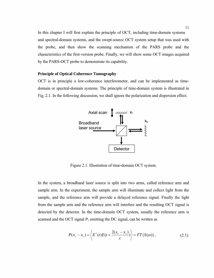
domain or spectral-domain systems. The principle of time-domain system is illustrated in
Fig. 2.1. In the following discussion, we shall ignore the polarization and dispersion effect.
Figure 2.1. Illustration of time-domain OCT system.
In the system, a broadband laser source is split into two arms, called reference arm and
sample arm. In the experiment, the sample arm will illuminate and collect light from the
sample, and the reference arm will provide a delayed reference signal. Finally the light
from the sample arm and the reference arm will interfere and the resulting OCT signal is
detected by the detector. In the time-domain OCT system, usually the reference arm is
scanned and the OCT signal P, omitting the DC signal, can be written as
)}({))(2
()()( * ωSFTc
xxtEtExxP sr
sr =−
+=− , (2.1)
Broadband laser source
Detector
xr
xs
Axial scan

12where E(t) is the electric field of the laser source, t is time, xr and xs are the optical path
lengths of the reference and sample arm, and c is the speed of light. Here we suppose the
light field is a wide-sense stationary random process. The interference signal is actually the
autocorrelation of the light field and depends only on the delay of the two arms, xr−xs, and,
according to the Wiener-Khintchine theorem, is the Fourier transform of power spectrum of
the laser. In the equation, FT{} denotes the Fourier transform and S(ω) is the power
spectrum of the laser. Thus, for a broadband source, the OCT signal only has significant
value when xr-xs is smaller than the coherence length. Suppose the sample is a mirror, then
the position of the mirror can be measured precisely. And if the sample has layered
structures, the positions of the different layers can also be measured. Thus the scanning of
the reference arm will provide an axial scan (A-scan) into the sample. And a 2D image of
sample can be obtained if we perform multiple A-scans (called a B-scan, as similar to
ultrasound imaging). According to the above discussion, we can see that the transverse
resolution is limited by the sample arm optics as in conventional microscope. The axial
resolution of OCT is limited by the coherence length of the laser source and inversely
proportional to the bandwidth of the source. For a source with spectrum of Gaussian
profile, the axial resolution can be expressed as [12]
λλ
π Δ=Δ
22ln2x , (2.2)
where λ is the center wavelength of the laser and Δλ is the bandwidth of the spectrum.
Thus the axial resolution is inversely proportional to the laser bandwidth, and OCT usually
requires broadband laser to achieve high axial resolution.
In the time-domain OCT system, the delay of light is scanned, and the OCT signal detected
directly corresponds to an A-scan into the sample. In spectral-domain OCT system,
however, the spectrum of the laser is measured or scanned to create the interference signal,
and the OCT signal has to be Fourier transformed to get the A-scan line. Spectral-domain
OCT systems can be spectrometer based or swept-source based, as shown in Fig. 2.2(a)(b).
The principles of these two variations are similar, and both will acquire the spectrum of the
interference signal. The interferometer setup is similar to Fig. 2.1, and the only difference is

13that the interference signal is obtained by the spectrometer or by scanning the
wavenumber k of the laser source instead of scanning the delay of reference beam.
Figure 2.2. Principle of spectral-domain OCT. (a) Spectrometer based OCT; (b) swept-source based OCT; (c) detected signal P(k) as the wavenumber k is sweeping; (c) Fourier transform of the detected signal P(k) gives the position information.
Suppose the laser source has a spectrum S(k). The optical power P(k), detected by the
spectrometer at different k or the detector when k is sweeping, can be written as
))(2cos()()(2)()()( srsrsr xxkkSkSkSkSkP −++= , (2.3)
Swept laser source with spectrum S(k)
Detector
xr
xs
Fourier Transform
k -2(xr-xs) x
)(kP )}({ kPFT
(a)
(c) (d)
2(xr-xs)
Broadband laser source
Spectrometer
xr
xs
(b)

14where Sr(k) and Ss(k) is the power returned from the reference mirror and the sample
mirror. A typical interferogram is shown in Fig. 2.2(c). The position information, xr-xs, can
then be obtained by Fourier transform of P(k):
))],(2())(2([
21*})()({2
)}({)}({)}({
srsrsr
sr
xxxxxxkSkSFT
kSFTkSFTkPFT
−−+−++
+=
δδ(2.4)
where * denotes convolution. Suppose the reference arm and the sample arm do not change
the light spectrum, then we can write Sr(k)=RrS(k) and Ss(k)=RsS(k), where Rr and Rs are
reflectance of reference and sample arm, respectively. Thus, equation (2.4) can be written
as
))],(2())(2([*)}({
)}({)()}({
srsrsr
sr
xxxxxxkSFTRR
kSFTRRkPFT
−−+−++
+=
δδ (2.5)
Thus, FT{P(k)} provides the axial position information of the sample, as shown in Fig.
2.2(d). From the equation we note that the width of the interference peaks are determined
by the Fourier transform of the laser spectrum S(k), similar as the time-domain case. Thus
the resolution of spectral-domain OCT is limited by the coherence length of the laser
source, just as in time-domain OCT. However, there is an important difference between
spectral-domain and time-domain OCT. From the equation and the figure, we note that for
the same sample position xs, there will be two peaks in the Fourier transformed axial scan
line. This phenomenon are called complex conjugate artifact [13] of spectral-domain OCT.
The artifact prevents the spectral-domain OCT from resolving the positive path length
difference from the negative one. Researchers have developed many methods [13, 14] to
resolve the artifact problem and expand the scan range of OCT. In our experiment, the
sample is positioned only in half of the space and we do not need to resolve the artifact
problem.
An important feature of spectral-domain OCT is that the discrete Fourier transform has to
be used in practice, which results in a fundamental scan range limit for an axial scan as the
15Fourier transform will be periodic. For systems without resolving the complex conjugate
artifact, the effective axial scan range can be written as [15]
k
xδπ
2max = , (2.6)
where δk is the spectral resolution of the sampling in k space.
Another important difference between the spectral-domain and time-domain OCT is the
phenomenon of SNR falloff as the optical path length difference between the reference arm
and sample arm gets larger [15, 16]. This is due to the finite linewidth of the swept source
in swept-source based system, and the finite pixel width of the array detector in the
spectrometer based system. In practice, this SNR falloff is less in swept-source system (~10
dB for the whole scan range in our swept-source system) than in spectrometer based system
(~20 dB for the whole scan range in our spectrometer based system) because of the narrow
linewidth of swept source.
Usually in an OCT system, the resolution and the sensitivity can be seriously affected by
dispersion mismatch between reference arm and sample arm [12]. In time-domain OCT,
we will have to make sure the dispersions of the two arms are matched for optimal results,
sometimes by inserting additional dispersion materials [17]. In spectral-domain OCT,
however, the dispersion compensation can be implemented by software algorithm [18].
This is another important advantage of spectral-domain OCT over time-domain OCT.
Nevertheless, in our swept-source OCT system, as the fiber SMF-28 (Corning) almost has
no dispersion around the working wavelength of 1300 nm, we do not need to do dispersion
compensation.
One of the most important reasons that the spectral-domain OCT become popular is its
SNR advantages over the time-domain OCT. Suppose the spectral-domain OCT acquire
signals in M evenly spaced k, then the SNR improvement over the time-domain system that
has the same laser power and same A-line scan rate is roughly M/2 [15], if shot noise
limited detection is assumed. A simple explanation for the SNR improvement can be
described as follows. The spectral-domain OCT acquire signals in M evenly spaced k, thus

16the corresponding position points in an A-scan is M/2, considering the complex
conjugate artifact. Suppose the spectral-domain OCT and the time-domain OCT has the
same acquisition time t for an A-scan, then the time for acquiring signal for one point is
Spectral-domain OCT: ttSDOCT = ,
Time-domain OCT: 2/M
ttTDOCT = ,
(2.7)
(2.8)
This is because in spectral-domain OCT, the whole A-scan line is always illuminated
during t. Instead, in time-domain OCT, the signal for a position point in A-scan line is only
collected when the reference beam scan to the equal-pathlength position. We know that the
SNR of the system is directly proportional to the acquisition time, and thus the SNR of the
spectral-domain OCT will be M/2 times higher than the time-domain OCT.
Experimental Setup of Swept-Source Based OCT System
In the experiment, we used a fiber based swept-source OCT system, as shown in Fig. 2.3.
The laser from the swept source (si425-1300-SL, Micron Optics.) went through a circulator
and was split by a 2 × 2 fiber coupler FC1. In the sample arm, the needle probe transmitted
and collected the light to and from the sample. The details of the needle probe, paired-
angle-rotation scanning (PARS) probe, will be explained in detail in the next section. In the
other output of FC1, another fiber coupler FC2 split the light into reference arm and trigger
generation module. The reference arm was made of a collimator and a mirror to reflect the
light back. A polarization controller was added to match the polarization of the reference
and sample beam to achieve optimal interference. The trigger generation module was used
to generate trigger signal for the analog-to-digital converter (ADC), the details of which are
shown in Fig. 2.4 and will be explained later. The light returned from the sample arm and
the reference arm were recombined at FC1 and the output two interference signals were
detected by a balanced detector. The ADC then sampled the signal according to the trigger
and sent it to the computer programs for data processing.

17
Figure 2.3. Experimental setup of swept-source based OCT. SMF: single-mode fiber; C: circulator; PC: polarization controller: ADC: analog-to-digital converter; FC1 and FC2: fiber coupler 1 and 2.
The two interference signals detected by the balanced detector can be written as, similar to
equation (2.3):
))(2cos()()(2)()()(1 srsrsr xxkkSkSkSkSkP −++= ,
))(2cos()()(2)()()(2 srsrsr xxkkSkSkSkSkP −−+= .
(2.9)
(2.10)
They were 180o out of phase, and the balanced detector detected the difference of the two
signals, which was
))(2cos()()(4)()()( 21 srsr xxkkSkSkPkPkP −=−= . (2.11)
In this way, the DC terms of the interference signals were canceled and the interference
term was doubled. Furthermore, the noise associated with the DC term, such as the power
fluctuation, will be canceled. Thus the balanced detection can significantly improve the
signal-to-noise ratio (SNR) of the system. Note that the beat noise, which is a component of
the excess noise, still cannot be removed by balanced detection [19], and will affect the
Sample
SMF
SMF SMF C Swept source
PC Needle probe
Reference arm
+ −
ComputerADC
Signal
Balanced detector
SMF
SMF Trigger generation module
Trigger
FC1
FC2
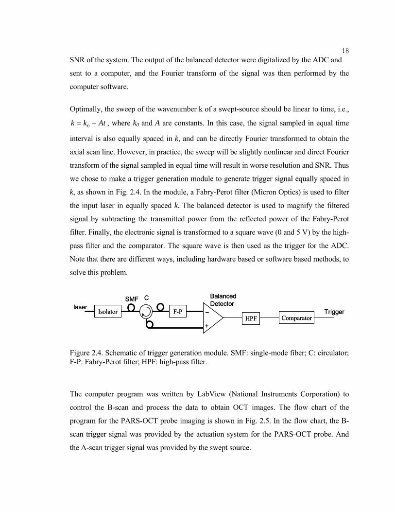
18SNR of the system. The output of the balanced detector were digitalized by the ADC and
sent to a computer, and the Fourier transform of the signal was then performed by the
computer software.
Optimally, the sweep of the wavenumber k of a swept-source should be linear to time, i.e.,
Atkk += 0 , where k0 and A are constants. In this case, the signal sampled in equal time
interval is also equally spaced in k, and can be directly Fourier transformed to obtain the
axial scan line. However, in practice, the sweep will be slightly nonlinear and direct Fourier
transform of the signal sampled in equal time will result in worse resolution and SNR. Thus
we chose to make a trigger generation module to generate trigger signal equally spaced in
k, as shown in Fig. 2.4. In the module, a Fabry-Perot filter (Micron Optics) is used to filter
the input laser in equally spaced k. The balanced detector is used to magnify the filtered
signal by subtracting the transmitted power from the reflected power of the Fabry-Perot
filter. Finally, the electronic signal is transformed to a square wave (0 and 5 V) by the high-
pass filter and the comparator. The square wave is then used as the trigger for the ADC.
Note that there are different ways, including hardware based or software based methods, to
solve this problem.
Isolator F-P
CSMF
+
−HPF Comparator
laserTrigger
BalancedDetector
Isolator F-P
CSMF
+
−HPF Comparator
laserTrigger
BalancedDetector
Figure 2.4. Schematic of trigger generation module. SMF: single-mode fiber; C: circulator; F-P: Fabry-Perot filter; HPF: high-pass filter.
The computer program was written by LabView (National Instruments Corporation) to
control the B-scan and process the data to obtain OCT images. The flow chart of the
program for the PARS-OCT probe imaging is shown in Fig. 2.5. In the flow chart, the B-
scan trigger signal was provided by the actuation system for the PARS-OCT probe. And
the A-scan trigger signal was provided by the swept source.

19The important characteristics of the swept-source based OCT system are summarized as
follows: laser power = 2.5mW, center wavelength = 1300nm, bandwidth = 70nm, axial
resolution = 9.3μm, A-scan rate = 250Hz, theoretical SNR = 125dB.
Start
Initialize Data Acquisition
Acquire one A-scan line data
Enough A-scans?No
YesProcess data
Display image and save file
End
Wait for B-scan trigger
Wait for A-scan trigger
Start
Initialize Data Acquisition
Acquire one A-scan line data
Enough A-scans?No
YesProcess data
Display image and save file
End
Wait for B-scan trigger
Wait for A-scan trigger
Figure 2.5. Flow chart of LabView program for the PARS-OCT probe imaging.
Paired-Angle-Rotation Scanning (PARS) Forward-Imaging Probe
The PARS-OCT probe is based on a pair of angle-cut gradient-index (GRIN) lenses. The
rotation of the GRIN lenses can deflect and scan the beam in the forward cone region ahead
of the probe tip. Similar as the side-imaging probe in [3], the actuation system is located
away from the probe tip, and thus allows easy miniaturization. We note that the GRIN
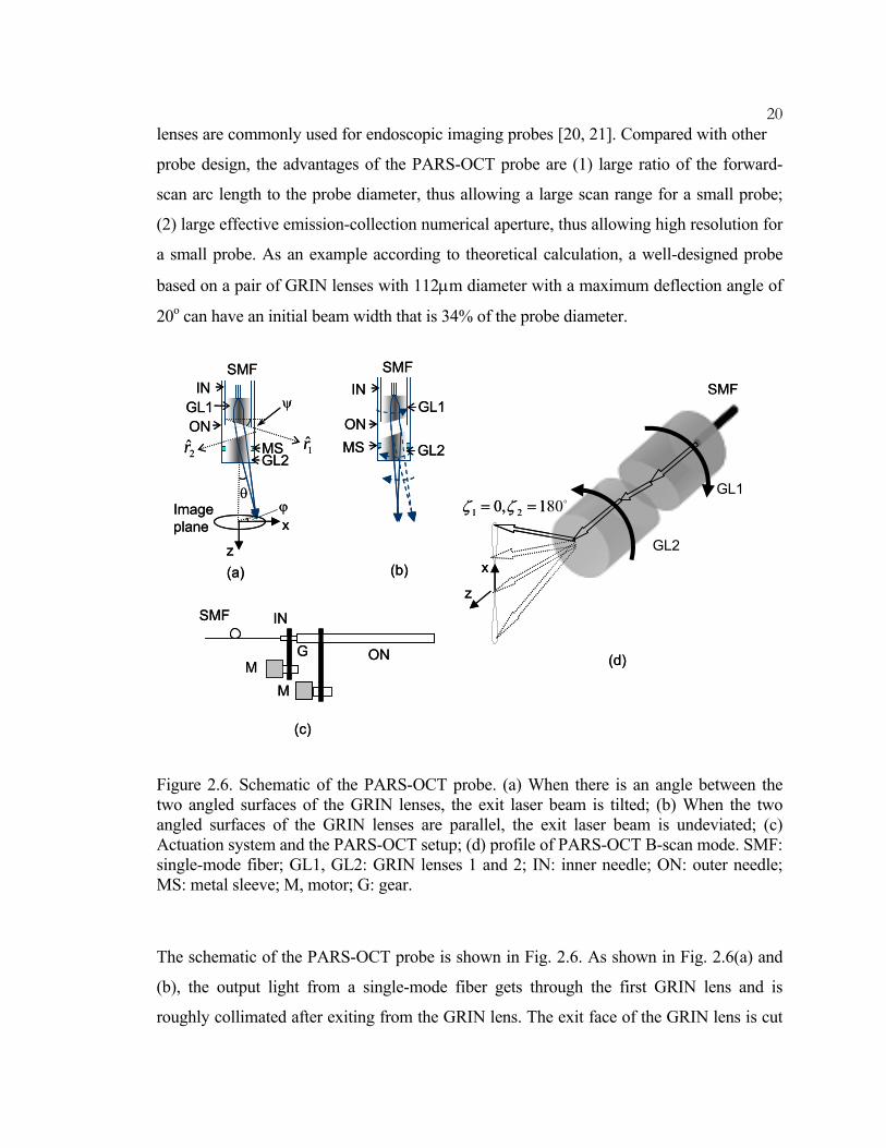
20lenses are commonly used for endoscopic imaging probes [20, 21]. Compared with other
probe design, the advantages of the PARS-OCT probe are (1) large ratio of the forward-
scan arc length to the probe diameter, thus allowing a large scan range for a small probe;
(2) large effective emission-collection numerical aperture, thus allowing high resolution for
a small probe. As an example according to theoretical calculation, a well-designed probe
based on a pair of GRIN lenses with 112μm diameter with a maximum deflection angle of
20o can have an initial beam width that is 34% of the probe diameter.
(c)
(d)
(b)(a)
ON
IN
GM
SMF
M
GL2
θϕ
GL1
GL2
SMFIN
ONMS
GL1
GL2
SMFIN
ONMS
GL1
SMF
z
xImage plane
2̂r 1̂r
x
z
o180,0 21 == ζζ
ψ
(c)
(d)
(b)(a)
ON
IN
GM
SMF
M
GL2
θϕ
GL1
GL2
SMFIN
ONMS
GL1
GL2
SMFIN
ONMS
GL1
SMF
z
xImage plane
2̂r 1̂r
x
z
o180,0 21 == ζζ
ψ
Figure 2.6. Schematic of the PARS-OCT probe. (a) When there is an angle between the two angled surfaces of the GRIN lenses, the exit laser beam is tilted; (b) When the two angled surfaces of the GRIN lenses are parallel, the exit laser beam is undeviated; (c) Actuation system and the PARS-OCT setup; (d) profile of PARS-OCT B-scan mode. SMF: single-mode fiber; GL1, GL2: GRIN lenses 1 and 2; IN: inner needle; ON: outer needle; MS: metal sleeve; M, motor; G: gear.
The schematic of the PARS-OCT probe is shown in Fig. 2.6. As shown in Fig. 2.6(a) and
(b), the output light from a single-mode fiber gets through the first GRIN lens and is
roughly collimated after exiting from the GRIN lens. The exit face of the GRIN lens is cut

21at an angle ψ, and thus the beam is deflected. The deflected beam then enters the second
GRIN lens through an identically angle-cut face of the GRIN lens, which further bends the
beam. Finally, the beam exits the second GRIN lens and focuses at a point ahead of the
probe. The exact position and the size of the focal point are determined by the pitches of
the two GRIN lenses. For convenience, we shall define the orientations of the two GRIN
lenses by angles ζ1 and ζ2, which are defined as the angles between the projections of
vectors 1̂r and 2̂r , respectively, in the image plane and the x-axis (see Fig. 2.6(a)). We shall
also define the direction of the output light beam by its polar angle θ that it makes with the
z-axis and its azimuthal angle ϕ; an angle of θ = 0 implies that the exit beam propagates
along the z-axis.
As shown in Fig. 2.6(a), when there is an angle between the two angled faces of the GRIN
lenses, the exit beam is tilted. For the special case of ζ1 = 0o and ζ2 = 180o, the exit beam
will have the largest deviation with θ = θmax and ϕ = 0. When the two GRIN lenses are
rotated simultaneously at the same speed and in opposite direction away from the starting
position of ζ1 = 0o and ζ2 = 180o, the exit beam will scan a fan sweep pattern, as shown in
Fig. 2.6(d), which can be used to acquire B-scan OCT images. Another special case is
when ζ1 = ζ2 = 90o, i.e., the two angled face of the GRIN lenses are parallel as shown in
Fig. 2.6(b), the exit beam will be undeviated. The two GRIN lenses are attached to separate
concentric needles, and the rotation of the two needles are actuated by two motors and
gears located far from the probe tip, as shown in Fig. 2.6(c).
The relation among θ, ζ1, and ζ2 cannot be simply expressed analytically. MATLAB
simulation of the probe trajectory during B scans (see Fig. 2.7) shows a consistent up-and
down sweep trajectory with acceptable deviation (the ratio of the maximum angle deviation
to the maximum sweep angle is 1.2%).

22
200 μm200 μm200 μm
Figure 2.7. Calculated B-scan mode profile as projected in the focal plane of the exit beam.
To get a simplified expression of θ, we assume that the beam is collimated by the first
GRIN lens, and then focused by the second GRIN lens. After the first GRIN lens, the angle
between the collimated beam and the axis is (α−ψ), where )sin(sin 1 ψα n−= . The ABCD
matrix of the GRIN lens can be written as [22], if we disregard the angled surface,
⎥⎥⎥⎥
⎦
⎤
⎢⎢⎢⎢
⎣
⎡
− )cos()sin(
)sin()cos(
2
1
2
0
0
1
AZnnAZ
nAN
AZAN
nAZ,
where N0 and A are the on-axis refractive index and the index gradient constant of the
GRIN lens, respectively, Z is the length of the GRIN lens, and n1 and n2 are the refractive
indexes of the medium before and after the GRIN lens, respectively. In paraxial region, the
ray direction (θin, θout) and height (hin, hout) before and after the GRIN lens, as indicated in
Fig. 2.8, can be calculated by the ABCD matrix as follows:
⎥⎦
⎤⎢⎣
⎡
⎥⎥⎥⎥
⎦
⎤
⎢⎢⎢⎢
⎣
⎡
−=⎥
⎦
⎤⎢⎣
⎡
in
in
out
out h
AZnnAZ
nAN
AZAN
nAZh
θθ )cos()sin(
)sin()cos(
2
1
2
0
0
1
. (2.12)
23
θin θouthin hout
GRIN lens
θin θouthin hout
GRIN lens
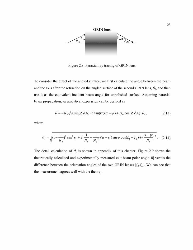
Figure 2.8. Paraxial ray tracing of GRIN lens.
To consider the effect of the angled surface, we first calculate the angle between the beam
and the axis after the refraction on the angled surface of the second GRIN lens, θ1, and then
use it as the equivalent incident beam angle for unpolished surface. Assuming paraxial
beam propagation, an analytical expression can be derived as
100 )cos())(tan()sin( θψαψθ ⋅+−⋅−= AZNdAZAN , (2.13)
where
2
0212
00
22
01 )()cos(sin))(11(2sin)11(
NNNNψαξξψψαψθ −
+−−−+−= . (2.14)
The detail calculation of θ1 is shown in appendix of this chapter. Figure 2.9 shows the
theoretically calculated and experimentally measured exit beam polar angle |θ| versus the
difference between the orientation angles of the two GRIN lenses |ζ1-ζ2|. We can see that
the measurement agrees well with the theory.

24
0 30 60 90 120 150 1800
5
10
15
20
|ζ1-ζ2|| θ
|
Calculationζ1-ζ2>0
ζ1-ζ2<0
Figure 2.9. Calculated and measured exit beam polar angle, |θ|, versus the difference between the orientation angles of the two GRIN lenses, |ζ1-ζ2|.
(a) (b)(a) (b)
Figure 2.10. Scanning modes of the needle probe. (a) Spiral scanning, when both needles rotate at slightly different speeds and in the same direction; (b) starburst scanning, when both needles rotate at slightly different speeds but in the opposite direction.
Since the PARS-OCT probe has two degrees of freedom for rotation, it is possible to scan
the exit beam across the whole forward cone region ahead of the probe tip. For example,
when both GRIN lenses rotate in the same direction with slightly different angular velocity
(in this case, θ changes slowly while ϕ changes quickly), the focal spot will trace out a
spiral, as shown in Fig. 2.10(a). In contrast, when both GRIN lenses rotate in opposite

25direction with a slightly different speed (in this case, θ changes quickly while ϕ changes
slowly), we can get a starburst scan pattern, as shown in Fig. 2.10(b).
0 100 200 3000.0
0.2
0.4
0.6
0.8
1.0
Nor
mal
ized
out
put p
ower
angle difference (degrees)
0 100 200 3000.0
0.2
0.4
0.6
0.8
1.0
Nor
mal
ized
out
put p
ower
angle difference (degrees)
Figure 2.11. The variation of the output power as the orientation of the needles changes.
3 cm3 cm
Figure 2.12. Actuation system and the PARS-OCT probe.
Because the refractive angle of the beam is changing during the rotation of the needles, the
output power of the probe depends on the orientation of the needle. We measured the
output power as the orientation of the needle changes for one of our prototype probes, as

26shown in Fig. 2.11. We can see from the data that the maximum variation is about 3 dB.
This will introduce some SNR difference for different scan lines, but the variation is still
acceptable for imaging.
In our prototype PARS-OCT probe, a pair of GRIN lenses (diameter = 1 mm, SLW-1.0
from NSG America) were polished to the desired length with an angle of ψ = 22o, then
attached, using common 5-minute epoxy, to an inner needle (18XTW gauge) and an outer
needle (16TW gauge) that are cut from standard hypodermic tubings (Poppers & Sons).
Thus the overall probe diameter is 1.65mm. A single-mode fiber (SMF) was then angled
cleaved (~8o) and attached to the back face of the GRIN lens in the inner needle. The back
face of the GRIN lens is also designed to be angled (~8o). Note that the purpose to angle
cleave the fiber and to used the angled GRIN lens is to reduce back reflection from the
inner reflection inside the needle, as this will contribute to the noise of the system and
reduce the SNR [23]. During fabrication, we rotated the fiber and monitored the back
reflection and made sure that the position of the fiber was optimal before applying epoxy.
To get a satisfactory SNR, the back reflection should be less than -45dB compared with the
exit laser power. For comparison, the return losses of fiber connectors are: PC > 45dB,
UPC > 50dB, APC > 60dB. Thus the back reflection of the probe should be at least better
than the PC connector to get a decent SNR. The exposed needle length was 1cm in the
prototype and can be easily adjusted to be up to 3cm long. Figure 2.12 shows a picture of
the actuation system and the prototype probe. The largest scan half angle θmax can be
calculated from ψ to be 19o. In our design, the on-axis pitch of the first GRIN lens (0.285)
is slightly larger than 1/4 so that the beam exits from the first GRIN lens was roughly
collimated (note that in this case a 1/4-pitch GRIN lens will generate a collimated beam,
and a 1/4 to 1/2-pitch GRIN lens will generate a converged beam) and thus insensitive to
the distance between the two GRIN lenses, which makes the fabrication easier. At the same
time, the slightly convergence of the beam helps to keep the beam within the probe
diameter although it is deflected. The on-axis pitch of the second GRIN lens (0.076) was
chosen to be shorter than 1/4 pitch so that the exit beam was focused tightly with the
desired working distance. ZEMAX simulation (ZEMAX Development) shows a focal spot
size of 9.3μm and a working distance of 1.15mm when the exit beam is undeflected. In

27comparison, the working distance of prototype probe was measured to be 1.4mm when
the exit beam is undeflected, and the focal spot size of the exit beam was measured to be
10.3μm. The difference is mainly caused by errors in the length GRIN lens during
polishing and approximated simulation of the angle-polished GRIN lens by Zemax. When
the exit beam is tilted at the position of ζ1 = 0o and ζ2 = 180o, the working distance will be
slightly shorter (1.27mm), and the focal spot size will be slightly larger (12.5μm).
Detector
Lens
r
Razor blade
z
Detector
Lens
r
Razor blade
z
Figure 2.13. Schematic of measuring the focus size of the exit beam.
The foal spot size was measured by moving a razor blade across the beam at different axial
locations to measure the beam size at the locations. As shown in Fig. 2.13, at one location
z, the power P(r) was measured versus the displacement r of the razor blade, and then the
curve P(r) was fit to an error function to get the beam size R(z). Finally the beam size data
at different locations R(z) were fit to a Gaussian beam intensity profile and to get the size of
the beam waist.
Because of the loss and internal reflections within prototype probe, the measured SNR of
OCT signal (93dB) is smaller than the theoretical value (125dB). The illumination power
on the sample was 450μW.

28
500 μm
(a) (b)
5 mmp
va
500 μm
(a) (b)
5 mmp
va
Figure 2.14. OCT image of the heart of a stage 54 Xenopus laevis. (a) Photograph of the needle probe and the tadpole in experiment. (b) OCT images acquired by the PARS-OCT probe. The pixel number is 320 (transverse) × 250 (axial). p: pericardium, v: ventricle, a: atrium.
To demonstrate the capability of the prototype probe, it was used to acquire images of the
Xenopus laevis tadpole. In the experiment, we rotated the two needles with equal and
opposite angular speeds (~21rpm). Fig. 2.14(a) shows the photograph of the needle and the
tadpole when acquiring the image. Figure 2.14(b) shows the OCT image of the heart of a
tadpole. We can clearly discern the pericardium, ventricle and atrium in the image. Note
that the image is transformed to a fan image because of the scanning profile of the probe.
By changing the initial position of the needles, we can perform B-scans in different
directions. As shown in Fig. 2.15, four B-scan images, at position 0o, 45o, 90o, 1350, are
acquired at the same position of the tadpole. Figure 2.15(a) shows the photograph of the
PARS-OCT probe and the tadpole when acquiring the images. Figure 2.15(b) shows the
scanned locations. The acquired images are displayed in Fig. 2.15(c)-(f). Each image has
350 A-scan lines and is acquired in 1.4s. The scan depth is 2.3mm. We can clearly see the
gill pockets of the tadpole in the images.

29
(a) (c) (d)
(e) (f)
5 mm
2.5 mm
(b)
cd
e f
500 μm
g
(a) (c) (d)
(e) (f)
5 mm
2.5 mm
(b)
cd
e f
500 μm(a) (c) (d)
(e) (f)
5 mm
2.5 mm
(b)
cd
e fcd
e f
500 μm500 μm
g
Figure 2.15. OCT images of the gill pockets of a stage 54 Xenopus laevis tadpole. (a) Photograph of the probe and the tadpole when acquiring the images. (b) Indication of the scan location (c)-(f) in the tadpole. (c)-(f) OCT images acquired by the PARS-OCT probe. g: gill pockets.
To characterize a forward-scanning probe, we shall define two important parameters, RDR
(scan range to probe diameter ratio) and BDR (beam diameter on the exit face to probe
diameter ratio):
,diameterProbe
faceexit on thediameter BeamBDR,diameter ProberangeScan RDR == (2.15)
where the scan range, probe diameter, and beam diameter on the exit face are indicated in
Fig. 2.16. Apparently, we would prefer larger RDR to get larger scan range for the same
probe diameter, and larger BDR to get a larger numerical aperture and thus better
transverse resolution. With an optimal design of the PARS-OCT probe, we can have RDR
= 3.6, and BDR = 0.3.

30
Figure 2.16. Definition of some parameters of the forward-scanning probe.
In summary, we have designed and implemented the paired-angle-rotation scanning
(PARS) OCT probe and demonstrated its capability by acquiring OCT images of the
Xenopus laevis tadpole. Compared with other OCT endoscopic probes, the PARS-OCT
probe has numerous advantages and can be easily miniaturized. The probe can be
potentially used in needle surgical procedures to provide high-resolution 3D tomographic
images of the targets forward of the probe.
References
1. D. Huang, E. A. Swanson, C. P. Lin, J. S. Schuman, W. G. Stinson, W. Chang, M. R. Hee, T. Flotte, K. Gregory, C. A. Puliafito, and J. G. Fujimoto, “Optical coherence tomography,” Science 254, 1178-1181 (1991).
2. Z. Yaqoob, J. Wu, E. J. McDowell, X. Heng, and C. Yang, “Methods and application areas of endoscopic optical coherence tomography,” Journal of Biomedical Optics 11, 063001 (2006).
3. G. J. Tearney, S. A. Boppart, B. E. Bouma, M. E. Brezinski, N. J. Weissman, J. F. Southern, and J. G. Fujimoto, “Scanning single-mode fiber optic catheter-endoscope for optical coherence tomography,” Optics Letters 21, 543-545 (1996).
4. X. D. Li, C. Chudoba, T. Ko, C. Pitris, and J. G. Fujimoto, “Imaging needle for optical coherence tomography,” Optics Letters 25, 1520-1522 (2000).
5. P. R. Herz, Y. Chen, A. D. Aguirre, K. Schneider, P. Hsiung, J. G. Fujimoto, K. Madden, J. Schmitt, J. Goodnow, and C. Petersen, “Micromoter endoscope catheter for in vivo, ultrahigh-resolution optical coherence tomography,” Optics Letters 29, 2261-2263 (2004).
6. X. M. Liu, M. J. Cobb, Y. C. Chen, M. B. Kimmey, and X. D. Li, “Rapid-scanning forward-imaging miniature endoscope for real-time optical coherence tomography,” Optics Letters 29, 1763-1765 (2004).
7. T. Q. Xie, H. K. Xie, G. K. Fedder, and Y. T. Pan, “Endoscopic optical coherence tomography with a modified microelectromechanical systems mirror for detection of bladder cancers,” Applied Optics 42, 6422-6426 (2003).
Scan range
Beam diameter on the exit face
Working distance
318. T. A. King, and G. M. Fuhrman, “Image-guided breast biopsy,” Seminars in
Surgical Oncology 20, 197-205 (2001). 9. C. P. C. Chen, S. F. T. Tang, T. C. Hsu, W. C. Tsai, H. P. Liu, M. J. L. Chen, E. Date,
and H. L. Lew, “Ultrasound guidance in caudal epidural needle placement,” Anesthesiology 101, 181-184 (2004).
10. J. Wu, M. Conry, C. Gu, F. Wang, Z. Yaqoob, and C. Yang, “Paired-angle-rotation scanning optical coherence tomography forward-imaging probe,” Optics Letters 31, 1265-1267 (2006).
11. S. Han, M. V. Sarunic, J. Wu, M. Humayun, and C. Yang, “Handheld forward-imaging needle endoscope for ophthalmic optical coherence tomography inspection,” Journal of Biomedical Optics 13, 020505 (2008).
12. B. E. Bouma, and G. J. Tearney, Handbook of optical coherence tomography (Informa healthcare, 2001).
13. M. V. Sarunic, M. A. Choma, C. Yang, and J. A. Izatt, “Instantaneous complex conjugate resolved spectral domain and swept-source OCT using 3x3 fiber couplers,” Optics Express 13, 957-967 (2005).
14. M. Wojtkowski, A. Kowalczyk, R. Leitgeb, and A. F. Fercher, “Full range complex spectral optical coherence tomography technique in eye imaging,” Optics Letters 27, 1415-1417 (2002).
15. M. A. Choma, M. V. Sarunic, C. Yang, and J. A. Izatt, “Sensitivity advantage of swept source and Fourier domain optical coherence tomography,” Optics Express 11, 2183-2189 (2003).
16. M. Wojtkowski, R. Leitgeb, A. Kowalczyk, T. Bajraszewski, and A. F. Fercher, “In vivo human retinal imaging by Fourier domain optical coherence tomography,” Journal of Biomedical Optics 7, 457-463 (2002).
17. I. Hartl, X. D. Li, C. Chudoba, R. K. Ghanta, T. H. Ko, J. G. Fujimoto, J. K. Ranka, and R. S. Windeler, “Ultrahigh-resolution optical coherence tomography using continuum generation in an air-silica microstructure optical fiber,” Optics Letters 26, 608-610 (2001).
18. M. Wojtkowski, V. J. Srinivasan, T. H. Ko, J. G. Fujimoto, A. Kowalczyk, and J. S. Duker, “Ultrahigh-resolution, high-speed, Fourier domain optical coherence tomography and methods for dispersion compensation,” Optics Express 12, 2404-2422 (2004).
19. A. M. Rollins, and J. A. Izatt, “Optimal interferometer designs for optical coherence tomography,” Optics Letters 24, 1484-1486 (1999).
20. W. A. Reed, M. F. Yan, and M. J. Schnitzer, “Gradient-index fiber-optic microprobes for minimally invasive in vivo low-coherence interferometry,” Optics Letters 27, 1794-1796 (2002).
21. J. C. Jung, and M. J. Schnitzer, “Multiphoton endoscopy,” Optics Letters 28, 902-904 (2003).
22. W. L. Emkey and C. A. Jack, “Analysis and Evaluation of graded-index fiber-lenses,” Journal of Lightwave Technology 5, 1156-1164 (1987).
23. K. Takada, “Noise in optical low-coherence reflectometry,” IEEE Journal of Quantum Electronics 34, 1098-1108 (1998).

32Appendix A: Derivation of Equation (2.14)
Figure 2A.1.Refraction at the angled face of the second GRIN lens. P1O is the incident ray, P3O is the refracted ray, and P2O is the surface normal.
The refraction happened at the angled face of the second GRIN lens can be illustrated in
Fig. 2A.1. Suppose the z-axis is along the axis of the GRIN lens, and the incident ray is at
the xz-plane. The incident ray is P1O, the refractive ray is P3O, and the surface normal is
OP2. We choose P1 and P2 such that OP1 = OP2 = 1, and P3 is at the line of P1P2. At small
angle approximation, |OP3| ≈ 1. We already know that the angle between incident ray P1O
and the z-axis is α-ψ, so the coordinates of P1 can be written as
))cos(,0),(sin( ψαψα −− . Assuming the angle between the projection of OP2 in the xy-
plane and the x-axis is φ, then the coordinates of P2 are )cos,sinsin,cos(sin ψφψφψ . Our
goal is to calculate the coordinates of P1, (x, y, z), such that the angle θ1 and the orientation
of the refractive ray can be calculated. Let γ be the angle between P1O and OP2, i.e., the
incident angle for refraction, and β be the angle between P3O and OP2, i.e., the refractive
angle. In small angle approximation, we have
x
z
y
O
P1
P2
P3

33
021
32 1NPP
PP≈≈
γβ . (2A.1)
Here we use the Snell’s law, and N0 is the center refractive index of the GRIN lens.
Obviously, the coordinates P1, P2, and P3 satisfy
.1
)cos(coscos
sinsinsinsin
)sin(cossincossin
021
32
NPPPP
zyx
≈=
−−−
=−
=−−
−ψαψ
ψφψ
φψψαφψ
φψ
(2A.2)
Here we use Eq. (2A.1). Thus
).cos(1cos)11(
,sinsin)11(
,)sin(cossin)11(
00
0
00
ψαψ
φψ
ψαφψ
−+−=
−=
−+−=
NNz
Ny
NNx
(2A.3)
So the angle θ1 satisfies
.)()(cossin)11(2sin)11(
)(sin)sin(cossin)11(2sin)11(
sin
2
000
22
0
20
2
00
22
0
22
3
22
11
NNNN
NNNN
yxOP
yx
ψαψαφψψ
ψαψαφψψ
θθ
−+−−+−≈
−+−−+−=
+≈+
=≈
(2A.4)
Now using the relation 21 ξξφ −= , we get the Eq. (2.14). Note that by knowing (x, y, z),
we can also calculate the azimuthal angle ϕ of the exit beam by
22
1cosyx
x+
= −ϕ . (2A.5)

34In the above calculation, we can also remove the approximations and calculated the θ1
and ϕ directly, although it will be a complicated expression. I used Matlab to simulate the
scanning of the PARS-OCT probe and the result is shown in Fig. 2.7.

35C h a p t e r I I I
FULL-FIELD PHASE IMAGING PRINCIPLE WITH HARMONICALLY MATCHED DIFFRACTION GRATING (G1G2 GRATING)
Compared with intensity imaging, quantitative phase imaging has the advantages of high
sensitivity and high resolution. Because phase techniques are sensitive to the optical path
length instead of the intensity change, they are widely used to study transparent samples,
such as living cells. Phase techniques can also be used in metrology as they can provide
higher resolution than intensity based techniques in many situations. The success of phase
contrast microscopy and differential interference contrast microscopy has proved the
efficacy of phase techniques in studying biological samples. The development of various
quantitative phase methods further shows the potential capacity of phase techniques in
many applications. In this chapter, I will focus on the full-field quantitative phase imaging
techniques that are developed in our lab using a harmonically matched diffraction grating
(G1G2 grating) [1-3]. Compared with other phase imaging methods, our technique has
many advantages: (1) Imaging speed is limited only by the camera’s speed, as phase image
are reconstructed from two camera images acquired simultaneously. In comparison, the
speed of phase shifting interferometry method is additionally limited by the phase stepping
process [4]. (2) Allowing full field-of-view phase imaging, unlike some other techniques
such as digital holography, where the tilt of reference beam can limit the field-of-view [5].
(3) The G1G2 grating is a planar device and can be easily designed and fabricated.
In the following sections I will first give an overview of the digital holography and the 3x3
fiber based interferometer. These two techniques are closely related to our phase-imaging
method. Then I will describe the details of the principle, fabrication process, and proof-of-
principle experiments of our technique. Further improvements and the application of the
technique on observing dynamics of biological samples will be shown in the next chapter.

36Overview of Related Phase-Imaging Techniques
Holography was invented by Gabor [6] about half a century ago and has been widely used
especially after the invention of laser. Conventional holography uses holographic materials
for recording the holograms. Recent years researchers began using digital recording
devices such as CCD cameras to record the holograms and can thus obtain quantitative
phase and intensity information of the sample. The technique is called digital holography
and its schematic is shown in Fig. 3.1.
Sample CCD
Sample beam
Reference beam
Sample CCD
Sample beam
Reference beam
Figure 3.1. Schematic of digital holography.
The interferogram on the CCD camera can be written as
**22 RSSRSRI +++∝ , (3.1)
where R and S are the complex amplitudes of the electric field of the reference beam and
the sample beam, respectively. The first two terms in Eq. (3.1) are DC terms, and the last
two terms are interference terms. After recording of the interferogram, the sample beam
can then be reconstructed by multiplying the reference field to the interferogram:
*2222 SRSRRSRRIR +++∝ . (3.2)
The first two terms are zero-order diffraction of the reference beam by the interferogram,
the third term is a replication of the original sample field except for a ratio coefficient, and
the last term is proportional to the conjugate of the sample field. To separate these different
components, the off-axis scheme is often adopted, where there is an angle between the

37reference beam and the sample beam. The angle will have to be large enough such that
the different components can be separated spatially and be small enough such that the high-
frequency fringes can be discerned by the CCD camera. The last two terms can then be
digitally propagated by the Fresnel integral to obtain the phase and intensity information of
the sample.
From the above description we can see that the off-axis scheme is critical for digital
holography. However, the high-frequency fringes on the CCD camera effectively result in
inefficient use of the pixels since several pixels have to be used to record one fringe that
contains both the phase and intensity information. The off-axis scheme also limits the
spatial resolution of the image because high resolution image corresponds to high spatial
frequency of the fringes, and the achievable frequency of the fringes is limited by the pixel
size of the CCD camera.
To overcome the abovementioned disadvantages of the off-axis holography, in-line
holography is also developed. In this case, a phase shifting is often used to extract the phase
information [7]. However, the phase-shifting process will need additional time and might
introduce additional noise.
To obtain the phase information without the phase-shifting process, 3 × 3 fiber coupler-
based technique has been developed [8, 9]. The schematic of the interferometer is shown in
Fig. 3.2.
Figure 3.2. Interferometer based on 3 × 3 fiber coupler
Sample beam
Reference beam
Port 1
Port 2
Port 3

38Assuming the 3 × 3 fiber coupler is ideal and the split ratio is the same for the output
ports, the interference signals at the output ports can be written as
Port 1: )3
2cos(32
331πψψ −−++= rssr
sr PPPP
P , (3.3)
Port 2: )cos(
32
332 rssrsr PP
PPP ψψ −++= ,
(3.4)
Port 3: )
32cos(
32
331πψψ +−++= rssr
sr PPPP
P , (3.5)
where Pr and Ps are the input powers of reference and sample beam, respectively; ψr and ψs
are the phases of the reference beam and sample beam before the fiber coupler. We can see
that the interference signals at the three output ports have a phase shift of 120o among one
another. This is effectively equivalent to a phase shifting interferometer and the phase and
intensity information can be easily calculated directly from the detected interference
signals.
We note that the 3 × 3 fiber coupler-based interferometer has to be combined with scanning
mechanism to acquire 2D images. This motivates us to look for its full-field equivalent
such that a 2D image can be obtained without scanning.
Harmonically Matched Diffraction Grating
Consider a simple interferometer as shown in Fig. 3.3(a), where a common beamsplitter is
used to split and combine the reference beam and the sample beam, the interference signals
at the output ports can be expressed as:
Port1: )cos(2/2/1 rssrsr PPPPP ψψ −++= ,
Port2: )cos(2/2/2 rssrsr PPPPP ψψ −−+= ,
(3.6)
(3.7)
where Pr and Ps are the reference power and sample power, respectively; ψr and ψs are the
phases of the reference beam and sample beam before incident on the beamsplitter. From
the equations we note that the interference terms are 180o out of phase with each other. As

39the two interference terms are trivially related, it is generally impossible to extract phase
information from this simple interferometer without resorting to some form of phase
encoding.
Sample beam
Reference beam
Port 1
Port 2
diffraction grating
Sample beam
x
zy
Reference beam
Port 1
Port 2
(a) (b)
Sample beam
Reference beam
Port 1
Port 2Sample beam
Reference beam
Port 1
Port 2
diffraction grating
Sample beam
x
zy
Reference beam
Port 1
Port 2
diffraction grating
Sample beam
x
zy
x
zy
Reference beam
Port 1
Port 2
(a) (b)
Figure 3.3. (a) Simple interferometer based on common beamsplitter; (b) interferometer based on single shallow grating.
The trivial phase shift of the two output ports can also be understood by noticing the
conservation of energy of the input and output power. Thus, in principle, the output of two
ports systems would be trivially related in phase. To get a nontrivial phase shift of the
interference signals, we note that multiport elements might be a good choice. Multiport
optical fiber coupler-based interferometry methods has been used to obtain nontrivial phase
shift of the interference signals, and phase information of the sample can be extracted, as
shown in the previous section. We know that diffraction grating is a good full-field version
of multiport beam splitter/combiner, and let us first take a look at the interferometer based
on a single shallow grating, as shown in Fig. 3.3(b). As is well known, a grating can confer
additional phase shifts to the diffracted beams [1]. For example, consider a sinusoidal phase
grating with transmittance:
))](2cos(exp[)( 0xxjxt +Λ
=πα , (3.8)

40where α is the amplitude of phase modulation, Λ is the period of the grating, x0 is the
displacement of the grating from the origin, and the grating is along the x-direction. The
transmittance can be expanded into Fourier series:
∑∞
−∞= ⎭⎬⎫
⎩⎨⎧ ++
Λ=
mm xxjmJxt ]
2)(2[exp)()( 0
ππα , (3.9)
where Jm(α) is the mth order Bessel function of the first kind. Thus, the phase shift of the
mth order diffraction is the phase of ⎭⎬⎫
⎩⎨⎧ +
Λ)
22(exp)( 0
ππα xjmJ m . For m > 0, we have
0)( >αmJ since α is small for shallow grating. So the phase shift is )2
2( 0ππ
+Λ
xm . For
m<0, the phase shift will be )2
2( 0ππ
+Λ
xm when m is even and πππ++
Λ)
22( 0xm when m
is odd (note that )()1()( αα mm
m JJ −=− ). By adding appropriate multiples of 2π, the phase
shift of the mth order diffraction can be written as
]2
2)[sgn()( 0
0ππ
φ +Λ
=x
mmxm , (3.10)
where sgn() is the sign function. In the special case of +1 and -1 order diffraction, the phase
shift with respect to the 0th order, can be written as
2
2)(,
22
)( 001
001
ππφππ
φ +Λ
−=+Λ
= −+
xx
xx , (3.11)
Hereon we will consider only the 0, +1 and -1 order of diffraction because the higher order
diffractions are usually much weaker.
Now return to the single grating based interferometer, the additional phase shift of the two
beams and the phase of interference signals can be described as shown in Fig. 3.4. Thus the
interference signal at the output ports can be written as:

41
Port 1: )2
2cos(2 111111
ππψψ +
Λ+−++=
xPPPPP rssrsr ,
Port 2: )2
2cos(2 1
22222ππ
ψψ −Λ
+−++=x
PPPPP rssrsr .
(3.12)
(3.13)
We can see that the interference signals also have a trivial phase difference of π. However,
the presence of a phase shift term Λ
12 xπ that is intrinsically related to the diffraction grating
is encouraging. As we will soon see, the G1G2 interferometer makes creative use of this
phase shift term to achieve nontrivial phase relationship between interferometer output
ports.
Figure 3.4. Additional phase shifts of the beams and of the interference signals in a single grating-based interferometer.
The G1G2 interferometer replaces the simple diffraction grating in the previous example
with a harmonically matched grating pair (G1G2 grating). The grating pair consists of two
gratings (called G1 and G2 grating, respectively) with periods Λ1, Λ2 that satisfy Λ1=2Λ2.
The G1G2 grating is used as a beam splitter/combiner in an interferometer setup, as shown
in Fig. 3.5.
2
2
1
1 ππ+
Λx
22
1
1 ππ+
Λ−
x2
2
1
1 ππ−
Λx
Single grating
S
R
1
2
x z
y Ports Order Phase Order Phase
Phases of interference signals
Reference beam Sample beam
22
1
1 ππ+
Λx
00
2
+11
-1 0 0

42
Figure 3.5. Additional phase shifts of the beams and of the interference signals in a harmonically matched grating (G1G2 grating)-based interferometer.
The additional phase of the diffracted beams φk,n (k=R, S represent the reference or sample
beam; n=1, 2 is the port number) are shown in the figure and can be written as, according
to Eq. (3.11),
,
22,
22
,2
2,0
1
11,12,
2
22,12,
1
11,11,21,01,
ππφφππ
φφ
ππφφφφ
+Λ
−==+Λ
−==
+Λ
====
−−
+
xx
x
GSGR
GSGGR
(3.14)
where φm,Gn is the additional phase shift of the mth diffracted order of the grating Gn; x1, x2
are the displacements of G1, G2, respectively. Thus the phases of interference signals and
their difference are
2
2
1
12,2,2
1
11,1,1
22,2
2Λ
+Λ
−=−=Δ+Λ
=−=Δxxx
RSRSππ
φφφππφφφ ,
2)(4
1
1212
ππφφφ −Λ−
=Δ−Δ=Δxx .
(3.15)
(3.16)
As long as Ζ∈⎟⎠⎞
⎜⎝⎛ +≠
Λ− nnxx ;
21)(4
1
12 ππ , we will have a nontrivial phase shift between
the output ports of the interferometer. By adjusting the relative displacement (x2-x1)
G1G2 grating 2
2
1
1 22Λ
+Λ
−xx ππ
S
R
xz
y 1
2
22
1
1 ππ+
Λx
22
2
2 ππ+
Λ−
x
Ports Order Phase Order Phase
Phases of interference signals
Reference arm Sample beam
22
1
1 ππ+
Λx
00
2
1
-1 (G2)
+1(G1)
22
1
1 ππ+
Λ−
x-1(G1)

43between G1 and G2 grating during fabrication, we can set the phase shift Δφ. Note that
the harmonic relation, Λ1 = 2Λ2, of the G1G2 grating is important. If this is not satisfied,
the diffraction beam of the G1 and G2 grating will not overlap, and the nontrivial phase
shift will not be uniform across the grating. It is further noted that besides the G1G2
shallow grating, the nontrivial phase shift of the interference signal can also be obtained by
gratings has deep relief [10]. However, unlike the shallow grating, the phase shift in the
deep relief grating depends on the polarization and wavelength of the incident light. Thus
we chose to use shallow grating for our demonstration of the idea.
Note that the harmonically matched gratings can also be separated in the interferometer, as
reported in [1]. In this case the displacement between G1 and G2 grating (x2-x1) can be
conveniently adjusted by a piezo actuator precisely. Nevertheless, for practical experiment,
we would like to make the G1G2 grating in one piece so that the phase shift is fixed and
insensitive to disturbance.
Because of the nontrivial phase shift between interference signals, we can calculate the
phase information of the sample beam. In this chapter, for a proof-of-principle study, we
will use the approximation that the reference power is much stronger than the sample
power. This requirement will be much less restricted in the improved algorithms described
in the next chapter. In this approximation, the detected powers at the output ports can be
written as
Port 1: )cos(2 1111 ψΔ+≈ srr PPPP ,
Port 2: )cos(2 2222 φψ Δ+Δ+≈ srr PPPP ,
(3.17)
(3.18)
where rs ψψψ −=Δ . Here we have omitted the additional phase shifts that are the same
for the two beams. Let 1,1
1,1
1
2
G
G
s
s
PP
+
−==ηη
η be the relative diffraction efficiency of the two
output ports, where Gnm,η denoting the efficiency of the mth diffraction order from grating
Gn (n=1, 2). Let

44
2
222
1
111 2
,2 r
r
r
r
PPPs
PPPs
η−
=−
= , (3.19)
then we have
11 )cos( sPs =Δψ ,
21 )cos( sPs =Δ+Δ φψ .
(3.20)
(3.21)
From Eq. (3.21),
21 )]sin()sin()cos()[cos( sPs =ΔΔ−ΔΔ φψφψ . (3.22)
By Eq. (3.20) and (3.22), we have
)sin(
)cos()sin( 211 φ
φψ
Δ−Δ
=ΔssPs . (3.23)
Thus by Eq. (3.20) and (3.23), we have the solution of the phase and amplitude of the
sample (relative to the reference) beam,
2
11
1
211
)cos(,
)sin()cos(tan ⎟⎟
⎠
⎞⎜⎜⎝
⎛Δ
=Δ−Δ
=Δ −
ψφφ
ψsP
sss
s . (3.24)
Thus in the experiment, we can calculate the phase and amplitude of the sample by
measuring the reference powers at the two detector, and then measuring the interference
signal simultaneously. The phase shift Δφ and the relative efficiency η are calibrated before
the experiment.
Experimental Setups
The G1G2 grating was created by recording three-beam interference on a PFG-01
holographic plate (Integraf LLC.), as shown in Fig. 3.6. A HeNe laser (Melles Griot,
~5mW output power, wavelength of 632.8 nm) was coupled by objective lens 1 into single
mode fiber to clean the beam. The output beam from the fiber was then expanded (power

45of 2.7 mW and diameter of 18 mm) by lens 1 and split into three beams. Beamsplitter 3
was inserted to make the power of the three beams match.
Figure 3.6. Experimental setup for recording the G1G2 grating. BS1-3: beamsplitter 1-3.
We arranged the beams to intersect at a standard 600 lines/mm grating. The angles between
the beams were adjusted such that the diffracted orders from different beams perfectly
overlapped (specifically, we overlap the 0, +1, and +2 orders from beam 1, 2, and 3,
respectively, into one spot; the -1, 0, and +1 orders from the same beams into a second
spot; and finally the -2, -1, and 0 orders into a third spot) and interfered to form bull’s eye
patterns. The adjustment made sure that the interferences among the three beams will form
two 600-line grating patterns and one 1200-line grating pattern at the position of the
standard 600 lines/mm grating. Note that the two 600-line grating patterns formed by beam
1, 2 and beam 2, 3 are equal in amplitude and might be displaced with respect to each
other. However, they will add up to form a single composite 600-line grating pattern. The
following is the mathematical derivation of the three-beam interference pattern. On the
interference plane, the three beams can be written as:
Beam 1: )exp()exp( 1101 θiyikEE y= , (3.25)

46Beam 2: )exp()exp( 2202 θiyikEE y= ,
Beam 3: )exp()exp( 3303 θiyikEE y= ,
(3.26)
(3.27)
where E0 is the amplitude of the electric field and is the same for all three beams; k1y, k2y,
k3y are the wave vector of the three beams in y-direction. θ1, θ2, θ3 are additional phases of
the three beams. Here we assume that the beam is in the yz-plane, and the interference
plane is at z = 0, and we omit the time variation term exp(-iωt). Thus the three-beam
interference pattern can be written as
],)cos[(
]2
)cos[(2
2cos23
])cos[(
])cos[(
])cos[(3
)()(
313120
1312
23120
20
313120
232320
121220
20
321*
321
θθ
θθθθθ
θθ
θθ
θθ
−+−+
−+−
−++=
−+−+
−+−+
−+−+=
++++=
ykkE
ykkEE
ykkE
ykkE
ykkEE
EEEEEEI
yy
yy
yy
yy
yy
(3.28)
where denotes the time average. The last step is because yyyy kkkk 2312 −=− . Finally
we have a 600-line grating (the yy kk 12 − term) and a 1200-line grating (the yy kk 31 −
term).
After the alignment, the grating was replaced with the PFG-01 holographic plate. We
exposed the plate to the overlapping beams for ~105 second (the time is chosen to optimize
the diffraction efficiency, according to the specified optimal exposure of ~110 μJ/cm2 and
the beam power and size) and processed the resulting plate to create the G1G2 grating.
A modified Mach-Zehnder G1G2 interferometer was then constructed for full field phase
imaging, as shown in Fig. 3.7. A HeNe laser (Thorlabs HRP120 with output power 12 mW
and wavelength of 632.8 nm) was focused by objective 1 (Swift 10X), and a pinhole
(diameter 25 μm) served as a spatial filter. The filtered laser beam was then collimated by
lens 1 (focal length 200 mm) and split by a 5/95 beam splitter so that most of the power

47will go to the sample arm. In the sample arm, objective lens 2 (Newport M-10X) and
lens 2 (focal length 200 mm) made up a microscope system that imaged the sample onto
two CCD cameras (The Imaging Source DMK 31BF03, 1024x768 pixels). The harmonic
grating pair served as the beam combiner/splitter. The distance between lens 2 and the
G1G2 grating was set at 90 mm. The maximum light intensity incident on the sample was
32.6 W/m2 and the light intensity of reference beam incident on the grating was 1.7 W/m2.
We measured %161,1 =+ Gη , %51,1 =− Gη and %92,1 =− Gη ; the diffraction efficiencies were
determined by the relative power of the light beams during the writing process.
CCD2
L1 S CCD1
BS O2 L2
Mirror
G1G2
HeNe
PO1
CCD2
L1 S CCD1
BS O2 L2
Mirror
G1G2
HeNe
PO1
Figure 3.7. The Mach-Zehnder interferometer setup for phase imaging. O1, 2: objective lens 1, 2; P, pinhole; L1, 2: lens 1, 2; BS: beam splitter; S: sample; G1G2: the harmonically matched grating pair (G1G2 grating) on a holographic plate.
The intrinsic interference phase difference of the grating, Δφ, was measured by sending a
narrow reference and sample beam (diameter ~1 mm) through the plate. The optical path
length of one arm was modulated by inserting an optical delay line (made up of a
retroreflector mounted on a voice coil and two right-angle prisms, as shown in Fig. 3.8)
into the setup. The interference signals were then read into computer for further phase
analysis by Hilbert transform. The uniformity of the phase difference across the plate’s
surface was verified by repeating the measurement at various points on the plate. Figure

483.9(a) shows the three line locations and Fig. 3.9(b) shows the measured nontrivial phase
shift for each line. Our measurements indicated good uniformity and a Δφ value of 75o±10o.
During imaging, P1 and P2 associated with each point on the image plane were measured.
Additionally, Pr1 and Pr2 were measured prior to imaging.
Voice coil moving
Retroreflector
Right-angle Prism
Voice coil moving
Retroreflector
Right-angle Prism
Figure 3.8. Optical delay line for modulating optical path length.
Figure 3.9. Nontrivial phase shift of interference signals measured in three different line locations of the G1G2 grating. (a) Indication of the three line locations; (b) measured nontrivial phase of each line.

49Proof-of-Principle Experiments
Figure 3.10. Phase image of double bars fabricated on an ITO glass with a thickness of 560nm. (a) Intensity image; (b) phase image; (c) schematic of the phase object; (d) quantitative phase value compared with the profilometry result. The dotted line and the solid line are measurements from our phase imaging system and profilometry, respectively.
To show the capability of the G1G2 interferometer, we used this system to image a phase
object consisting of two bars of polymethyl methacrylate (PMMA) material (width of 75
μm, separation of 75 μm, and height of ~560 nm) on an indium tin oxide (ITO) coated
glass plate, as shown in Fig. 3.10(c). The phase object was fabricated by e-beam
lithography. The acquired intensity and phase images are shown in Fig. 3.10(a), (b). We
can see that the intensity image (Fig. 3.10(a)) shows little contrast. However, the features of
the objects are clearly visible in the phase image (Fig. 3.10(b)). Given the refractive index n

50of PMMA (n = 1.496 at the wavelength of λ = 632.8 nm), the thickness of the bar t can
be calculated from the measured phase difference Δθ inside and outside the bar as
)1(2 −Δ
=n
tπ
θλ , (3.29)
Quantitative measurement of the PMMA thickness (~540 nm) is shown in Fig. 3.10(d); the
data agree well with the profilometry measurement (~555 nm). The standard deviation of
the data shown in Fig. 3.10(d) is ~33 nm, which corresponds to a phase error of ~9.3o.
The phase imaging system was then used to observe liquid diffusion in a microfluidic
channel, as shown in Fig. 3.11. The study of fluidic interfaces in microfluidic channels is
important for numerous applications [11]. Micromixing is usually observed through the use
of dyes. These techniques are indirect, as it is the movements of the dye molecules rather
than the actual fluid molecules that are observed. Phase imaging techniques enable the
direct observation of fluid mixing as long as the fluids involved have different refractive
indices (r.i.). Fig. 3.11(a) shows the fabricated microfluidic channel for observing the
mixing of three fluid streams. In the experiment, a NaCl solution was pumped (weight
percentage = 30%, r.i. = 1.393) into the middle inlet of the channel and two streams of
deionized water were pumped (r.i. = 1.333) into the two side inlets. The flow speed was
1m/minute inside the microfluidic channel. Phase (Fig. 3.11(e)-(g)) and intensity (Fig.
3.11(b)-(d)) images were acquired in the junction region and two downstream locations as
indicated in Fig. 3.11(a). Once again, the intensity images showed little contrast while the
phase images clearly showed the diffusion of the fluids in the channel. This experiment
demonstrates the utility of our phase imaging technique to study fluid mixing in
microfluidic systems.

51
Figure 3.11. Observing the diffusion process in a microfluidic channel. (a) Microfluidic channel for 3 fluids mixing. W: water; S: salt water. The location of acquired images is indicated. (b)-(d) Intensity images acquired in three different locations as indicated in (a); (e)-(g) Corresponding phase images of (b)-(d).
In summary, we have shown the principle and proof-of-principle experiments of the full-
field phase imaging system based on G1G2 interferometer. The heart of the G1G2
interferometer is the G1G2 grating –– a harmonically matched grating pair. The G1G2
grating can confer nontrivial phase shift between output interference signals at different
output ports, and thus quantitative phase and intensity information associated with a
transmissive sample can be measured directly without temporal, spatial, or polarization
encoding. In experiments of this chapter, the samples for phase imaging are relatively
simple and lack of detail structures and are just for proof of principle. In next chapter, I will
show the improvements of the optical system and apply the technique to acquire images of

52biological samples with detail structures and also acquire video for observing movement
of the sample.
References
1. Z. Yaqoob, J. Wu, X. Cui, X. Heng, and C. Yang, “Harmonically-related diffraction gratings-based interferometer for quadrature phase measurements,” Optics Express 14, 8127-8137 (2006).
2. J. Wu, Z. Yaqoob, X. Heng, L. M. Lee, X. Cui, and C. Yang, “Full field phase imaging using a harmonically matched diffraction grating pair based homodyne quadrature interferometer,” Applied Physics Letters 90, 151123 (2007).
3. J. Wu, Z. Yaqoob, X. Heng, X. Cui, and C. Yang, “Harmonically matched grating-based full-field quantitative high-resolution phase microscope for observing dynamics of transparent biological samples,” Optics Express 15, 18141-18155 (2007).
4. T. Zhang and I. Yamaguchi, “Three-dimensional microscopy with phase-shifting digital holography,” Optics Letters 23, 1221-1223 (1998).
5. K. J. Chalut, W. J. Brown, and A. Wax, “Quantitative phase microscopy with asynchronous digital holography,” Optics Express 15, 3047-3052 (2007).
6. D. Gabor, “Microscopy by reconstructed wave-fronts,” Proceedings of the Royal Society of London. Series A, Mathematical and Physical Sciences 197, 454-487 (1949).
7. I. Yamaguchi, T. Zhang, “Phase-shifting digital holography,” Optics Letters 22, 1268-1270 (1997).
8. M. A. Choma, C. Yang, and J. A. Izatt, “Instantaneous quadrature low-coherence interferometry with 3x3 fiber-optic couplers,” Optics Letters 28, 2162-2164 (2003).
9. Z. Yaqoob, J. Fingler, X. Heng, and C. Yang, “Homodyne en face optical coherence tomography,” Optics Letters 31, 1815-1817 (2006).
10. C. M. B. Cordeiro, L. Cescato, A. A. Freschi, and L. Li, “Measurement of phase differences between the diffracted orders of deep relief gratings,” Optics Letters 28, 683-685 (2003).
11. J. Atencia and D. J. Beebe, “Controlled microfluidic interfaces,” Nature 437, 648-655 (2005).

53C h a p t e r I V
PHASE IMAGING OF BIOLOGICAL SAMPLES WITH G1G2 INTERFEROMETRY
In the previous chapter I explain the basic principles of the full-field imaging technique
based on G1G2 interferometer and show some proof-of-principle experiments. It has been
demonstrated that the G1G2 interferometer is potentially useful for many applications that
require high-resolution quantitative phase imaging. However, previous implementation of
the G1G2 interferometer has a couple of design issues that limit this technique when it is
applied for high-resolution imaging. First, there are geometric aberrations in the raw data
image from the output ports when high spatial resolution (1.6 μm) and moderate field of
view (400 × 300 μm) are required. As a consequence, the coincidence mapping of raw data
images is difficult beyond a certain resolution limit. Second, the phase computation
algorithm previously employed required the sample beam to be much weaker than the
reference beam. This requirement will affect the dynamic range of the system.
In this chapter, I will show the improvement of aberration issue by updating the optical
setup and the improvement of the dynamic range by improving the data processing
algorithm [1]. Finally I will show the result of some preliminary experiments of the phase
imaging system on acquiring phase images of biological samples and acquiring video of
moving samples.
Improved Experimental Setup for Imaging Biological Samples
First let us take a look at the aberration issue of the imaging system in previous setup, as
shown in Fig. 4.1. In the setup, a diffraction grating was put in the imaging space to diffract
one of the output imaging beams. The inherent distortion that such geometry introduced
can be appreciated by considering the imaging of a point source as the sample, as shown in
Fig. 4.1(a). We notice that the beam will converge prior to transmission through the
grating. As the angle of diffraction associated with the grating does not linearly depend on
the incident angle, we can expect to observe geometric aberration in the image. And the

54amount of aberration depends on the numerical aperture of the imaging space. To
determine the extent of distortion, we used ZEMAX (ZEMAX Development Corporation)
to simulate this scenario. In the simulation, we assumed the objective and the lens were
perfect paraxial lens so that the aberration observed could be solely attributed to the
diffraction grating. As shown in Fig. 4.1(b), when we increase the distance between the
imaging plane and the lens, we can observe the image transit from a vertical focus (left) to
a horizontal focus (right). This phenomenon is similar to astigmatism. Fig. 4.1(e) shows the
transmission image of a letter “C” pattern acquired using the system shown in Fig. 4.1(a),
where the location of the imaging plane was selected to give us vertical focus. The blur in
the horizontal direction is readily observable.
To correct this astigmatic aberration in the improved optical setup, we employed the
imaging scheme shown in Fig. 4.1(c), where the grating was put between the objective and
the lens. In this case, the incident light associated with each point on the object plane was
transformed into a collimated beam at the grating. The collimated beams would diffract
from the grating as collimated beams. These would then transform back to point objects in
the image plane by passing through the lens. Our ZEMAX simulations confirmed this fact
(see Fig. 4.1(d)). Fig. 4.1(f) shows the image of the same letter “C” acquired using this
setup, with which we can easily see that the obvious astigmatism aberration had been
removed.
We experimentally determined the resolution of this imaging system to be equal to 1.6 μm
(Sparrow’s criterion) by measuring the image profile of an effective point source (a hole of
diameter 150 nm). The measured resolution agreed well with the theoretically calculated
value of 1.2 μm based on the imaging system parameters.

55
sample
objective
grating
lens
imaging plane
sample
objective
grating
lens
imaging plane
(a)
(e)
(b)
(f)(c)
Increasing imaging plane distance
(d)objective
grating
lens
imaging plane
(g)
sample beam
Airy disk
20 μm
20 μm
400
μm
400
μm
Airy disk
Inte
nsity
(a.u
.)In
tens
ity (a
.u.)
sample
objective
grating
lens
imaging plane
sample
objective
grating
lens
imaging plane
(a)
(e)
(b)
(f)(c)
Increasing imaging plane distance
(d)objective
grating
lens
imaging plane
(g)
sample beam
Airy disk
20 μm20 μm
20 μm20 μm
400
μm
400
μm
Airy disk
Inte
nsity
(a.u
.)In
tens
ity (a
.u.)
Figure 4.1. Geometric aberration induced by the grating. (a) Previous imaging setup. (b) Astigmatism of the focal spots of previous setup. (c) Current imaging setup. (d) No aberration in the focal spot of current setup. (e) Image of letter “C” acquired by the previous setup. (f) Image of letter “C” acquired by the current setup. (g) Aberration of illumination beam caused by the grating diffraction in current setup.
This updated setup confers aberrations onto the input collimated light that is used to
illuminate the sample (see Fig. 4.1(g)). This is because the collimated light will be focused

56by the objective and will diverge when it enters the grating. The aberration of
background beam will introduce unwanted pattern in the interferograms and unwanted
phase aberration in the final phase image. Fortunately, we can measure and characterize
this phase aberration during initial system calibration by removing the sample. This
systematic error can then be removed from actual sample image measurements during data
processing.
sample
objective
grating
lens
imaging plane stretch
compression
stretch
compression
sample
objective
grating
lens
imaging plane stretch
compression
stretch
compression
Fig. 4.2. “Stretch” and “compression” distortion caused by the diffraction of the grating in the imaging system.
Another aberration issue associated with the grating diffraction that we need to be
concerned about is the spatial “stretch” and “compression” distortion on the off-axis
diffracted raw data image due to the diffraction process. As shown in Fig. 4.2, the image
will be stretched in one direction and compressed in the other direction, and this effect is
opposite for +1 and -1 order diffraction of the grating.

57This distortion in principle will affect the matching of the two CCD images. However,
the following calculation shows that the effect is small enough and can be neglected. The
distortion is due to the fact that the angle of diffraction associated with the grating does not
linearly depend on the incident angle. Mathematically, a point that is x1 away from the
center of object field will be mapped to a point x2 from the image field’s center, as shown
in Fig. 4.3. The figure shows only the chief ray, and the lenses and the grating is centered
and perpendicular with respect to the chief ray from the center of object field. Suppose the
lenses are perfect paraxial, then we have, according to the figure,
),tan(,)sin(sin
,tan
,sin
0222
21
111
0
θθλθθ
θ
λθ
−==+
=
=
fxd
fxd
(4.1)
where f1, f2 are the focal length of the objective and the lens, respectively; λ is the
wavelength of the laser; d is the grating period; and the angles are indicated in the figure.
The above equations can be solved to get x2, as given by
⎥⎦
⎤⎢⎣
⎡−⎟⎟
⎠
⎞⎜⎜⎝
⎛−= −−−
dfx
dfx λλ 1
1
11122 sin)sin(tansintan . (4.2)
As x2 is not linearly dependent on x1, the resulting image will appear distorted. When x1 is
small, the above equation can be simplified as
12212
2/1
/ xdffx
λ−
−= , (4.3)
where x2 is proportional to x1 and there is no distortion. Note that the magnification is given
by 22
12
1
2
/1
/
d
ffxx
λ−
−= , and is larger than that of a simple microscope system without the
grating, which is 1
2
ff
− . However, the difference is small since d is usually several times of
λ. In our experimental setup, f1 = 16.5mm, f2 = 200mm, λ = 632.8nm, d = 1/600mm. For

58the field of view with a maximum offset, x1 = 0.16mm, the difference between the two x2
calculated by Eq. (4.2) and (4.3) is 4.5 μm, which is smaller than the size of a pixel on the
CCDs (pixel size = 4.7μm). Beyond this field of view, the distortion does cause a slight
deterioration in resolution. This problem can be resolved by appropriate spatial rescaling of
the raw data images.
sampleobjective
grating
lens
imaging plane
θ1
θ2
θ0x1
x2
sampleobjective
grating
lens
imaging plane
θ1
θ2
θ0x1
x2
Fig. 4.3. Calculation of the “stretch” and “compression” distortion.
According to the previous analysis, we built our improved optical system setup as shown in
Fig. 4.4. A HeNe laser (Thorlabs HRP120, with output power of 12 mW and wavelength of
632.8 nm) was split into reference beam and sample beam. In the reference arm, the laser
was spatial filtered and expanded by objective 1 (Newport M-10X), a pinhole (diameter of
25 μm) and lens 1 (focal length of 200 mm). The transmitted and diffracted reference
beams were then collimated by lenses 3 and 4, respectively. The focal lengths of lenses 2,
3, and 4 were all equal to 200 mm. In the sample arm, objective 2 (Olympus UPlanFl 10X)
and lens 3 (lens 4) made up the microscope system that imaged the sample onto the CCDs
(The Imaging Source DMK 31BF03, 1024×768 pixels). The harmonically matched grating
pair (G1G2 grating) served as the beam splitter/combiner. The G1G2 grating is the same as
the one used before and is antireflection coated.
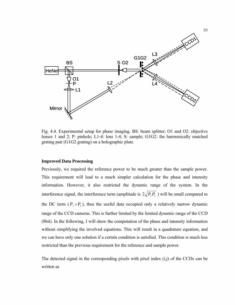
59
L1
S
CCD1
BS O2
L4
Mirror
G1G2
HeNe
PO1
CCD2
L3
L2L1
S
CCD1
BS O2
L4
Mirror
G1G2
HeNe
PO1
CCD2
L3
L2
Fig. 4.4. Experimental setup for phase imaging. BS: beam splitter; O1 and O2: objective lenses 1 and 2; P: pinhole; L1-4: lens 1-4; S: sample; G1G2: the harmonically matched grating pair (G1G2 grating) on a holographic plate.
Improved Data Processing
Previously, we required the reference power to be much greater than the sample power.
This requirement will lead to a much simpler calculation for the phase and intensity
information. However, it also restricted the dynamic range of the system. In the
interference signal, the interference term (amplitude is sr PP2 ) will be small compared to
the DC term ( sr PP + ), thus the useful data occupied only a relatively narrow dynamic
range of the CCD cameras. This is further limited by the limited dynamic range of the CCD
(8bit). In the following, I will show the computation of the phase and intensity information
without simplifying the involved equations. This will result in a quadrature equation, and
we can have only one solution if a certain condition is satisfied. This condition is much less
restricted than the previous requirement for the reference and sample power.
The detected signal in the corresponding pixels with pixel index (i,j) of the CCDs can be
written as

60 )),(cos(),(),(),(),(),( 11111 jijiPjiPAjiPjiPjiP srsr ψΔ++= , (4.4)
),),(cos(),(),(),(
),(),(),(),(
12
122
φψη
η
Δ+Δ+
+=
jijiPjijiPA
jiPjijiPjiP
sr
sr (4.5)
where Pr1(i, j) and Pr2(i, j) are the reference powers at the pixels of CCD1 and CCD2,
respectively; Ps1(i, j) and Ps2(i, j) are the sample powers at corresponding pixels of the
CCDs; ),(/),(),( 12 jiPjiPji ss=η is the relative diffraction efficiency of the grating for the
sample beam; A is the interference factor determined by the coherence of the laser, ideally
A=2, in practice, the measured A is 1.9; ranabeobj jijiji θψψψ ++=Δ ),(),(),( , where
),( jiobjψ is the optical phase change associated with presence of the sample, ),( jiabeψ is
the phase aberration background introduced by the grating as mentioned in the previous
section, ranθ is some random phase attributable to environment fluctuation and independent
of pixel index (i, j); Δφ is the nontrivial phase shift between the interference signals caused
by the G1G2 grating and is independent on the pixel index (i, j). To get the phase and
intensity information, the experiment procedure for phase extraction can be designed as
follows:
1) Determine the relative diffraction efficiency η(i, j).
2) Determine the phase aberration ),( jiabeψ and the nontrivial phase shift Δφ. This
involves acquiring N (we use N = 100) frame pairs of the interferograms in the absence of
the sample. For pixel (i, j) (i = 1,…,1024, j = 1,…,768) of the CCD k (k = 1, 2), we can get
a time series yi,j,k(n), n = 1…N. For different n, there is a different random phase introduced
by environmental disturbance. Since the time series for any of the two pixels has a phase
difference between them, if we plot one time series versus another, we will get an elliptical
profile. For the time series from the same CCD, we can let the first pixel (i = 1, j = 1) be the
reference point and compute the phase difference for each CCD pixel with respect to the
reference point by performing elliptic fitting [2] between yi,j,k(n) and y1,1,k(n). This

61computed phase difference is equal to the phase aberration abeψ . Similarly, by
performing elliptic fitting between the corresponding pixels from the two CCDs, yi,j,1(n)
and yi,j,2(n), we can get the phase shift Δφ. The procedure of elliptic fitting can be briefly
explained as follows. Suppose we have signals x and y that can be measured as
),cos()(
,cos)(
22
11
φθθθθ
++=+=
AByABx
(4.6)
then the plot of y versus x will be an ellipse. By canceling θ and rearranging the equation,
we can get
06542
322 =+++++ ayaxayaxyax , (4.7)
where
.sincos2
,cos22
,cos22,,cos2
221
2
12122
22
212
16
2
1122
212
5
2
21142
2
21
32
12
φφ
φ
φφ
AA
ABBA
BABa
ABA
AAB
a
ABA
BaAA
aAA
a
−−+=
+−=
+−==−=
(4.8)
The coefficients a2 to a6 are then obtained by fitting the measured data of x and y to
equation (4.7) using least-square fitting. Then the phase shift φ can be extracted by
)2
(cos3
21
aa
−= −φ . (4.9)
Figure 4.5 shows an example of the elliptic fitting of the two time series of signals from
two pixels.
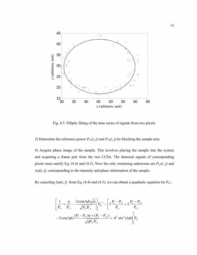
62
Fig. 4.5. Elliptic fitting of the time series of signals from two pixels.
3) Determine the reference power Pr1(i, j) and Pr2(i, j) by blocking the sample arm.
4) Acquire phase image of the sample. This involves placing the sample into the system
and acquiring a frame pair from the two CCDs. The detected signals of corresponding
pixels must satisfy Eq. (4.4) and (4.5). Now the only remaining unknowns are Ps1(i, j) and
Δψ(i, j), corresponding to the intensity and phase information of the sample.
By canceling Δψ(i, j) from Eq. (4.4) and (4.5), we can obtain a quadratic equation for Ps1:
122
21
2211
2
22
1
1121
2121
)(sin)()(
)cos(2
22)cos(21
srr
rr
r
r
r
rs
rrrr
PAPP
PPPP
PPP
PPP
PPPPP
⎥⎥⎦
⎤Δ+
−+−Δ−
⎢⎣
⎡ −+
−−
⎥⎥⎦
⎤
⎢⎢⎣
⎡ Δ−+
φηη
φ
ηφη
30 35 40 45 50 55 60 6515
20
25
30
35
40
45
x (arbitrary unit)
y (a
rbitr
ary
unit)

63
0))(()cos(2)()(
21
2211
2
222
1
211 =
⎥⎥⎦
⎤
⎢⎢⎣
⎡ −−Δ−
−+
−+
rr
rr
r
r
r
r
PPPPPP
PPP
PPP
ηφ
η.
(4.10)
For clarity, we omitted the functional dependency on (i, j) in the expression. This equation
yields two solutions for Ps1. In order to be able to choose only one solution, the sample
power Ps1 need to satisfy some condition, which is derived as follows.
To begin, assume the sample power solution is s0 and the other solution of equation (4.10)
is s1, then we have
.)cos(21
)(sin)()()cos(222
2121
22
21
2211
2
22
1
11
10
rrrr
rr
rr
r
r
r
r
PPPP
APP
PPPPP
PPP
PP
ssηφη
φηη
φ
Δ−+
Δ+−+−
Δ−−
+−
=+ (4.11)
If we always have s1>s0, then we can choose the smaller solution of the equation and get s0
that we want. So we should have
.)cos(21
)(sin)()(
)cos(2222
2121
22
21
2211
2
22
1
11
0
01
rrrr
rr
rr
r
r
r
r
PPPP
APP
PPPPP
PPP
PP
s
ss
ηφη
φηη
φ
Δ−+
Δ+−+−
Δ−−
+−
<⇒
>
(4.12)
Substitute P1 and P2 from equation (4.4), (4.5), where Ps1 = s0, we get
)(sin
2)()(
)cos(
)cos(21
22
21
2211
2
22
1
11
21210
φηη
φ
ηφη
Δ+−+−
Δ−−
+−
<
⎟⎟⎠
⎞⎜⎜⎝
⎛ Δ−+
APP
PPPPP
PPP
PP
PPPPs
rr
rr
r
r
r
r
rrrr

64
)(sin2
)]cos([)]cos([cos
)cos()cos(
22
21
020010
2
020
1
010
φη
φψηηηψφ
φψηηψ
Δ+Δ+Δ++Δ+
Δ−
Δ+Δ++
Δ+=
APP
sPAssPAs
PsPAs
PsPAs
rr
rr
r
r
r
r
0)(sin2
)sin(sin)sin()sin( 22
2
0
1
0 >Δ+ΔΔ−Δ+ΔΔ⇒ φψφη
φψφ AP
sAPsA
rr
.
(4.13)
Without loss of generality, we can let 0)sin( >Δφ , thus
0)sin(2
)sin()sin(2
2
0
1
0 >Δ+Δ−Δ+Δ φψη
φψ AP
sAPsA
rr
.0)sin(2
)cos()sin()sin()cos(2
1
0
2
0
1
0 >Δ+ΔΔ+Δ⎥⎥⎦
⎤
⎢⎢⎣
⎡−Δ⇒ φψφψ
ηφ A
PsA
PsA
PsA
rrr
(4.14)
If for all Δψ, the above equation is satisfied, we must have
),(sin4
)cos(2
0)sin(2
)sin()cos(
22
2
2
1
1
2
2
1
1
22
1
0
2
2
0
1
0
φφ
φφη
φ
Δ<Δ−+⇒
>Δ+⎥⎥⎦
⎤
⎢⎢⎣
⎡Δ+
⎥⎥⎦
⎤
⎢⎢⎣
⎡−Δ−
APP
PP
PP
PP
APsA
PsA
PsA
r
s
r
s
r
s
r
s
rrr (4.15)
where Ps1 = s0 and Ps2 = ηs0. Thus if the above equation is satisfied, we can always use the
smaller solution of the quadratic equation (4.10) as our solution. For the ideal quadrature
phase shift, Δφ=90o and ideal coherence, A=2, the above condition becomes
12
2
1
1 <+r
s
r
s
PP
PP . (4.16)
This condition still requires smaller sample powers compared with the reference powers.
However the condition is much less restricted than the requirement of previous system.
Having obtained the solution for the sample power Ps1, we can then calculate the phase

65term Δψ by substituting Ps1 in Eq. (4.4) and (4.5). The phase of the sample plus some
uniform random phase is then given by aberanobj ψψθψ −Δ=+ .
The term ranθ tends to be constant over the entire image but it can vary in time. One
approach to remove it from a time sequence of phase images is to look at the variation of
ranobj θψ + at a location in the image where it is known that objψ is not varying. The time
dependent variations can then be wholly attributed to ranθ . We can then subtract this value
from each image at each time point. This is the approach we employed when we generated
phase image movie sequences.
We note that step 1 through 3 need only be done once during calibration. Thus the image
acquisition time is only limited by the frame rate of the CCD cameras.
Fig. 4.6. Compare unwrap algothms. (a) Wrapped image; (b) unwrapped image by simple unwrap algorithm; (c) unwrapped image by Flynn’s algorithm.
Next we will need to deal with the phase wrapping of phase images when the optical path
length difference is greater than the wavelength. Due to the presence of noise in the phase
image, simple unwrap algorithm (where a phase jump of more than π will be adjusted by
adding or subtracting multiple of 2π so that the jump become smaller than π, and the
processing is based on 1D unwrapping) generally does not work well. For our experiment,
we instead chose to use the Flynn’s minimum discontinuity algorithm [3], which is 2D
technique, to unwrap the image. Flynn’s algorithm operates by identifying the lines of
discontinuities and joining them into loops. Appropriate multiples of 2π are then added to

66each pixel enclosed by the loops to remove the phase wrap discontinuities. This unwrap
algorithm worked well for our data. Figure 4.6 shows an example of the application of
unwrap algorithms to our data. Figure 4.6(a) shows the wrapped phase image acquired by
our system. Figure 4.6(b) shows an unwrapped phase image as generated by the simple
unwrap algorithm. Figure 4.6(c) shows that the Flynn’s algorithm is capable of better phase
unwrapping performance.
Phase Noise Analysis
We can estimate the phase noise in the shot noise limit theoretically as follows. To simplify
the problem, we assume that the reference powers and sample powers are the same for the
two output ports. We also assume the interference factor A = 2 and the nontrivial phase
shift Δφ = -90o. Now the power detected in the two output ports can be written as
ψΔ++= cos21 srsr PPPPP ,
ψΔ++= sin22 srsr PPPPP .
(4.17)
(4.18)
So
srsr PPPPP −−=Δ 1cos2 ψ ,
srsr PPPPP −−=Δ 2sin2 ψ .
(4.19)
(4.20)
For noise analysis, we may assume the detected power P1 and P2 contain additive Gaussian
white noise terms x1, x2 with zero mean, respectively. For the detect power P1, the
corresponding electron number of the CCD is
11 Ph
nν
ητ= , (4.21)
where h is the Planck’s constant, ν is the light frequency, η is the quantum efficiency of the
CCD, and τ is the exposure time. For shot noise, which obeys the Poisson distribution, the
standard deviation of n1 is proportional to the square root of the average n1 [4], i.e.,

67
11P
hn νητσ = . (4.22)
So the corresponding standard deviation in P1 can be written as
111Phh
nx ητν
ητνσσ =⋅= . (4.23)
Similarly
22Ph
x ητνσ = . (4.24)
P1-Pr-Ps
P2-Pr-Ps
2σx1
2σx2
δψsr PP2
ψ
P1-Pr-Ps
P2-Pr-Ps
2σx1
2σx2
δψsr PP2
ψ
Fig. 4.7. Schematic of the phase noise assessment.
Thus as shown in Fig. 4.7, the phase noise can be approximately expressed as
.
222
)sin(cos22
21
221
2221
sr
srsr
sr
srsr
srsr
xx
PPPPPPh
PPPPPPh
PPPPh
PP
++≤
Δ+Δ++=
+=
+≈
ητν
ψψητ
νητ
νσσδψ
(4.25)

68For a typical set of numbers for our system, Pr = 5 nW, Ps = 1.5 nW, η = 0.9, τ = 100 μs,
we have δψ ≤ 2 mrad.
In the experiment, we measure the phase stability of our system by using a cover glass as
the sample and measuring the phase difference between two different spots on the cover
glass. The phase of the spots is the average of the pixels in the spots with corresponding
object size of 1.2 μm x 1.2 μm, matching the diffraction limit of the objective lens. The
sample power incident on each spot was 1.6 nW (port 1) and 1.5 nW (port 2). The
reference power incident on each spot was 7.6 nW (port 1) and 3.1 nW (port 2). The
exposure time per image frame was 100 μs. The experiment results are shown in Fig. 4.8.
The phase image is shown in Fig. 4.8(a), and the fluctuation of the phase difference versus
time is shown in Fig. 4.8(b). The phase stability of our system is characterized by the
standard deviation of the fluctuation, which equals 62 mrad (corresponding to 6.24 nm
optical path length).
Fig. 4.8. Measurement of the temporal phase stability. (a) Phase image of a cover glass, the two spots that are used to measure the phase stability are indicated; (b) Fluctuation of the phase of spot 2 with respect to spot 1 versus time, the standard deviation is 62 mrad.
We note that the phase noise in shot noise limit is much less than the measured phase noise
(62 mrad) in the experiment. This might be due to the vibration of the optical components
0 5 10
-0.2
0
0.2
time (sec)
phas
e (ra
d)
(a) (b)
std=62mradspot 1
spot 2 Phas
e (ra
d)

69in the system during the exposure time of the camera. Actually, if we assume a power
fluctuation of 3%, i.e., 21 03.0,03.021
PP xx == σσ , then the phase noise can be calculated
as
.2)(44)(2
015.0
)sin(cos)(44)(2015.0
015.02
2
2
221
22221
sr
srsrrsr
sr
srsrrsr
srsr
xx
PPPPPPPPPP
PPPPPPPPPP
PPPP
PP
++++≤
Δ+Δ++++=
+=
+≈
ψψ
σσδψ
(4.26)
Substituting the typical powers employed in the experiment, we find that δψ ≤ 80 mrad,
which is comparable with the phase error measured in the experiment.
In addition to the phase stability characterization, this set of experiments revealed another
aspect of this experimental scheme –– we can see some dim fringes in the phase image in
Fig. 4.8(a). These fringes were caused by the relative larger phase noise near some special
phase locations. For a simple explanation, consider the quadratic equation (4.10),
aPs12+bPs1+c=0, where a, b, c are the coefficients shown in the equation, the solutions are
acbwherea
bPs 4,2
21 −=Δ
Δ±−= . (4.27)
The error of the solutions can be written as the function of the measured error of P1, P2:
.
22/)/(/
22/)/(/
222
111
22
11
1
11
Pa
PPbPa
PPb
PPP
PPP
P sss
δδ
δδδ
Δ∂Δ∂±∂∂−+
Δ∂Δ∂±∂∂−=
∂∂
+∂∂
= (4.28)
Thus, when Δ is small, the error of the solution will be large. The fringes in Fig. 4.8(a)
correspond to locations where this effect occurred. Fortunately, in our experiments, this

70additional phase noise was relatively small (~0.2 rad) and showed up in only a small
region of the image.
Application in Phase Imaging of Biological Samples
Fig. 4.9. Images of “CIT” logo by our iamging system. (a) Intensity image; (b) phase image; (c) 3D reconstruction of the phase image; (d) step-height measurement.
As an initial demonstration of our system, we performed phase imaging of a phase object,
which consisted of a “CIT” logo written on a 100 nm thick polymethyl methacrylate
(PMMA). As expected, the intensity image shown in Fig. 4.9(a) had little contrast. In
comparison, the phase image (Fig. 4.9(b)) had excellent contrast. Figure 4.9(c) shows the
3D reconstruction of the phase image. The measured height of a step is shown in Fig.

714.9(d); the thickness of the logo was measured to be 114±12 nm, which agreed well with
the thickness measurement performed with a standard profilometer.
Fig. 4.10. Images of onion skin cells. (a) Intensity image; (b) phase image; (c) 3D reconstruction of the phase image.
We next used our system to image onion skin cell (Fig. 4.10). The intensity and phase
images are shown in Fig. 4.10(a), (b), respectively. Figure 4.10(c) shows the 3D
reconstruction of the phase image. Again, the phase image has much better contrast than
the intensity image, and the optical thickness of the cell can be quantitatively measured
from the phase image. The nuclei can be seen clearly in the phase image.

72
Fig. 4.11. Phase images of a moving amoeba proteus at four different times (t = 0, 3, 6, 9 seconds). The sizes of the images are 147 μm (width) × 123 μm (height) (372 × 312 pixels).
Finally, we applied our system to observe the movement of an amoeba proteus. As the
phase image can be reconstructed from two camera images obtained simultaneously, the
frame rate of the acquired video is limited by the frame rate of the CCDs. We use a
functional generator to externally trigger the two CCDs to control the frame rate according
to the movement of the sample. For the amoeba proteus observed, the frame rate was set to
be 10 frames/second. Figure 4.11 shows the phase images of a moving amoeba proteus at
four different times (t = 0, 3, 6, 9 seconds), in the figure we can clearly see the nucleus and
contractile vacuole of the amoeba. We can also see the movement of the pseudopodiums.
In summary, we have shown the improvements of the G1G2 interferometer based phase-
imaging technique, including improvements in optical system setup and in data processing.
We also explain the detail studies on geometric aberrations and phase noise. Applying the
improved phase-imaging system to acquire images of standard samples and biological

73samples shows the capability of the system on high-resolution phase imaging. We also
verify the possibility of using the technique to observe dynamics of biological samples.
Because the acquisition speed is only limited by the frame rate of the cameras, our phase-
imaging technique is applicable for observing fast dynamics and is potentially useful for
biomedical studies.
References
1. J. Wu, Z. Yaqoob, X. Heng, X. Cui, and C. Yang, “Harmonically matched grating-based full-field quantitative high-resolution phase microscope for observing dynamics of transparent biological samples,” Optics Express 15, 18141-18155 (2007).
2. M. Pilu, A. W. Fitzgibbon, and R. B. Fisher, “Ellipse-specific direct least-square fitting,” Proceedings of IEEE International Conference on Imaging Processing 3, 599-602 (1998).
3. D. G. Ghiglia and M. D. Pritt, Two-Dimensional Phase Unwrapping: Theory, Algorithms, and Software, Section 4.5 (John Wiley & Sons, 1998).
4. A. Yariv, Optical Electronics in Modern Communications (Oxford University Press, 1997).

74C h a p t e r V
FRESNEL ZONE PLATE BASED PROJECTION IN OPTOFLUIDIC MICROSCOPY
Our group has developed the technique of optofluidic microscopy (OFM) during the last
few years [1-3]. Combined with the appropriate high flow-velocity microfluidic techniques
[4], OFM systems can potentially address a large number of biomedical applications, such
as image-based cytometry, blood parasite diagnosis and water quality inspection. The OFM
imaging approach differs significantly from the conventional microscopy approach; the
design choice is motivated by the fact that the conventional microscope design, with its
requisite high precision optical elements, is difficult to miniaturize cost-effectively.
In this chapter, I will describe the use of Fresnel zone plate (FZP) to project the aperture
images onto the imaging sensor for acquiring OFM images [5]. I will explain the principles
of OFM, the design and fabrication of the FZP, and show the experimental setup of FZP-
OFM and imaging results.
Principles of Optofluidic Microscopy (OFM)
The basic idea of the OFM is to scan the shadow of the sample under light illumination
using tiny apertures to reconstruct the microscopic image. The transmissions through the
tiny apertures are either directly collected by an imaging sensor underneath the apertures or
projected by imaging system onto the imaging sensor. The scanning motion is achieved by
flowing the sample through a microfluidic channel. The size of the microfluidic channel
can be designed to constraint the distance from the sample to the aperture, and thus increase
the resolution. Unlike direct shadow imaging [6], the size of the aperture can be chosen to
be much smaller than the pixel size of the imaging sensor and thus can achieve high-
resolution imaging. Since one aperture can only contribute to one line scan across the
sample, we need to use an aperture array to scan the whole sample as it flows through the
microfluidic channel. Each transmission time trace of the aperture in effect represents a line
scan across the sample. By compiling all of the line scans appropriately, we can create a

75microscope image of the sample in which the optimal resolution is fundamentally limited
by the aperture size.
Flow direction Flow direction
(a) (b)
δy δyθ
x
ySample
Flow direction Flow direction
(a) (b)
δy δyθ
x
ySample
Figure 5.1. Two possible arrangements of the aperture array direction with respect to the flow direction of the sample. (a) The aperture array direction is perpendicular to the flow direction; (b) The aperture array direction has is tilted at an angle θ with respect to the flow direction.
One of the most obvious ways to arrange the aperture array is shown in Fig. 5.1(a), where
the direction of the array is perpendicular to the sample flowing direction. The coordinate
system is also shown in the figure. In this way, the line scans from the apertures can be
directly put together to get the image of the sample. As can be seen from the figure, the
vertical scan step (δy) is determined by the distance of the adjacent apertures (L): δy = L.
To achieve high resolution, δy, and thus L, must be chosen to be equal or smaller than the
resolution limit. For example, if we want to achieve a resolution of 1 μm, L should be equal
or less than 1 μm. However, this is not easy to implement for the following reason. For
apertures directly on top of the imaging sensor, each aperture must be fabricated on top of
one pixel. But the pixel size of the sensor is generally greater than 1 μm. For projection
based OFM, high-resolution optical imaging systems are required to differentiate distance
of 1 μm. However, the additional optical imaging system is generally bulky. To overcome
this limitation, we choose to arrange the aperture array so that it is tilted at an angle θ with
respect to the flow direction, as shown in Fig. 5.1(b). In this case the vertical scan step is

76 θδ sinLy = . (5.1)
Thus we can set a small tilt angle θ to make δy satisfy the resolution limit and still allow L
to be large enough for easy imaging. For example, in my experiment, we choose L = 10μm
and θ = 3.3o, and thus δy = 0.6μm. The vertical scan step δy will be the y-direction pixel
size in the final OFM images.
Because of the tilted arrangement of the aperture array, each line of the reconstructed
image is actually a time-shifted line scan from the corresponding aperture. The time shift
between adjacent line scans Δt can be expressed as
V
Lt θcos=Δ , (5.2)
where V is the flow speed of the sample inside the microfluidic channel. And the x-
direction pixel size of the final OFM image can be calculated as
FVx =δ , (5.3)
where F is the frame rate of the imaging sensor. Suppose the length of the sample is l, then
the image acquisition time can be expressed as
Vltj
VljLT +Δ=
+=
θcos , (5.4)
where j is the total number of apertures that scan the sample.
During the experiment, the flow speed V can be measured by an α-hole and a β-hole, which
will scan the same part of the sample [1, 5], as explained later in this chapter. Another
possible way to measure the flow speed is to use multiple aperture arrays to acquire OFM
images [2], which could achieve a better precision.
In its typical format [2], an OFM system consists of three parts: an array of apertures
patterned on a metal-coated linear array sensor, a microfluidic channel emplaced on the

77aperture array such that the aperture array spans the channel floor in a skewed pattern,
and a uniform light field projected through the microfluidic channel to the aperture array.
This lensless design allows us to build highly compact and high-resolution microscope
systems with commercially available CMOS and CCD sensor chips in a simple and cost-
effective way.
While the typical OFM design calls for the aperture array to be patterned directly onto a
metal-coated linear array sensor, there are certain scenarios for which a different OFM
design, where the aperture array and the sensor are separated, would be preferable. Here are
two of the more important scenarios: 1) Recycling/retrieval of optical sensor is desired. The
typical OFM structure is not particularly easy to dismantle. If the optical sensor employed
is inexpensive, this would not be an important consideration as the complete replacement
of an entire expended OFM system would be more cost-effective. On the other hand, if the
cost of optical sensor employed is high, an OFM design that allows easy disassembly and
recovery of the optical sensor would be highly desirable. 2) Cooling of the optical sensor is
desired. Operating an optical sensor at a low temperature can help reduce noise and
improve signal-to-noise ratio. While cooling the OFM optical sensor to sub-freezing
temperatures is easily achievable, the close proximity of the aperture array and the
microfluidic channel to the optical sensor implies that that such cooling will likely freeze
the microfluidic channel content as well. As such, an OFM design in which the aperture
array and the microfluidic channel are well separated from the optical sensor is desirable in
such a scenario. The OFM scheme that is explained in this chapter falls into this category
of OFM design.
Besides the abovementioned typical designs for OFM, there are also other OFM
configurations that could be possibly implemented, such as illumination type OFM, grid
based OFM, surface plasmon polaritons (SPP) assisted OFM, OFM with a fiber bundle,
and fluorescence OFM [7].
The physical resolution of the OFM system can be characterized by the point spread
function (PSF) associated with the imaging aperture. We can achieve an optimal resolution

78determined by the aperture size when the sample is very close to the aperture (in the
optical near field regime). Since the width of the PSF increases as the height of the point
object increases, the resolution of our OFM system will degrade with increasing distance
between the sample and the aperture. The PSF can be measured by laterally scanning a near
field scanning optical microscope (NSOM) tip across the aperture at different height H and
measure the transmitted signals through it [8]. Figure 5.2 shows the schematic of measuring
the PSF. For the 1μm aperture used in my experiment, we measured the width of the PSF
to be 0.9 μm when H = 0.1 μm and 3 μm when H = 2.5 μm. Thus the ultimate resolution of
my OFM system is 0.9 μm.
Figure 5.2. Schematic for measuring the PSF of the aperture. NSOM tip is scanning above the aperture and a microscope relay collects the transmitted light into the detector.
Another important issue in OFM is the actuation mechanism for the sample scanning. Since
OFM is a scanning based microscope, the successful OFM imaging relies on the stability of
sample flowing, and we must ensure that the sample does not rotate or change shape during
the imaging process. Currently the mechanisms that have been used in OFM are pressure
driven flow [1], gravity driven flow [2, 5], electroosmosis flow [2] in the microfluidic
channel, and optical tweezer in fluidic chamber [3]. All these methods have their own
advantages and disadvantages. In my project, I chose to use the gravity driven flow as it is
NSOM tip
Microscope relay
Detector
Aperture

79relatively simple and the flow speed is appropriate for our imaging speed. During the
experiment, the flow stability can be monitored by the α-hole and a β-hole, as explained
later.
Note that OFM is an aperture based technique. The idea of aperture scanning can also be
used for other applications, such as beam profiler [9] and differential interference contrast
microscopy [10] that were developed in our lab.
Characteristics of Fresnel Zone Plate and Its Fabrication
The Fresnel zone plate (FZP) is a classic diffractive optical element that can be used to
focus light and used as a lens. It can be considered as a circular diffraction grating with
radially increasing line densities, each circular ring is called a zone. Similar to a grating, the
FZP has multiple diffraction orders. The FZP can be amplitude modulated or phase
modulated, as shown in Fig. 5.3. The basic idea is to introduce an optical path difference of
λ)21( −l (where l is integer, the diffraction order is 2l-1) between adjacent zone boundaries
so that the transmission through the zones will have a constructive interference. For
amplitude FZP, the zones are alternatively blocked. For phase FZP, the adjacent zones have
λ/2 optical thickness difference. Suppose the radius of boundary of the mth zones is rm, it
can be calculated by considering a collimated light incident on the FZP. To get a
constructive interference at the focus F, the optical path difference (OPD) between adjacent
zone boundaries should satisfy
λ)21(2
1222 −=+−+= − lrfrfOPD mlml , (5.5)
where fl is the (2l-1)th order focal length and λ is the wavelength. In paraxial
approximation, lm fr << , thus the above equation can be approximated as
λ)21()
21()
21( 2
21
2
2
−=+−+ − lf
rf
fr
fl
ml
l
ml . (5.6)

80So
...).,3,2(
12)0(
)12()12(
101
20
221
2
=−
===⇒
−+=⇒−+= −
llf
fandrfmr
flmrrflrr
lm
lmlmm
λ
λλ (5.7)
Here we let r0 = 0. So rm can be calculated providing the +1 order focal length f1. In the
following we will only consider the +1 order diffraction and let f = f1. During our imaging
by FZP, the image is formed by +1 order diffraction and other diffraction orders contribute
to the background of the image.
F
f
rm F
f
rm
(a) (b)
F
f
rm F
f
rm
(a) (b)
Figure 5.3. Schematic of the Fresnel zone plate (FZP). (a) Amplitude FZP; (b) phase FZP. F: focus, f: focal length, rm: the radius of boundary of the mth ring.
To consider the contrast of the image by FZP, we will need to know the efficiency of +1
order diffraction. The diffraction efficiencies of the FZP can be calculated by the Fresnel
diffraction approximation [11]. For amplitude FZP, the +1 order diffraction efficiency is
1/π2, and thus most of the power will contribute to the background of the image, especially
the 0 order diffraction, which has 1/4 of incident power. To increase the diffraction
efficiency of +1 order and thus the contrast of the image, we chose to use the phase FZP.
For phase FZP, the +1 order diffraction efficiency is 4/π2 and there will be no 0 order
diffraction.

81Beyond the paraxial region, the FZP will have serious aberrations for extended objects
[12, 13]. For this reason, and also the existence of multiple diffractions, FZP is seldom used
as imaging lens especially in the visible regime where better conventional refractive optics
are available. Nevertheless, as the FZP in our FZP-OFM design is only used to project the
transmissions from the apertures onto an optical sensor, the OFM resolution (dependent on
the aperture size) is unaffected by the FZP’s aberration characteristics as long as the
transmission projections from the apertures are differentiable. Finally, we note that it is
possible to design a general diffractive optical element (DOE) other than the FZP to
increase the imaging performance in nonparaxial region [14]. However, the resulting DOE
is generally more complicated and requires more efforts to design and fabricate.
As the FZP can be cost-effectively fabricated with current microfabrication techniques such
as optical or electron-beam lithography, the manufacturing cost associated with this OFM
design is anticipated to be low. And the FZP-OFM system can be made very compact
because of the small size of the FZP.
In our experiment, the FZP was designed to have a focal length of f = 800 μm. The radius
of the mth zone was calculated by Eq. (5.7). Our FZP has 32 zones with an outer diameter
of 255 μm. The radii of the zones are shown in the following table.
Table 5.1 Radii of the zones of the Fresnel zone plate
Nth zone Radius (μm) Nth zone Radius (μm) 1 22.5 17 92.8 2 31.8 18 95.5 3 39.0 19 98.1 4 45.0 20 100.6 5 50.3 21 103.1 6 55.1 22 105.5 7 59.5 23 107.9 8 63.6 24 110.2 9 67.5 25 112.5
10 71.2 26 114.7 11 74.6 27 116.9 12 77.9 28 119.1 13 81.1 29 121.2 14 84.2 30 123.2 15 87.1 31 125.3 16 90.0 32 127.3

82The zone number and the outer diameter are designed according to the focal length and
the resolution limit of the photolithography (~2 μm) used in our system. Before the
fabrication of FZP, the design was sent to the UCLA nanolab for fabrication. Figure 5.4
shows the prefabricated chrome mask of FZP.
Figure 5.4. Chrome mask of the Fresnel zone plate.
glassSU-8
glassSU-8
FZP pattern
glassSU-8
Aluminum
glassSU-8
AluminumSPR220-7
glassSU-8
Aluminum
(a)
(b)
(c)
(d)
(e)
glassSU-8
glassSU-8
FZP pattern
glassSU-8
Aluminum
glassSU-8
AluminumSPR220-7
glassSU-8
Aluminum
(a)
(b)
(c)
(d)
(e)
Figure 5.5. Fabrication procedure of our FZP.

83To reduce stray light from transmitting through the peripheral of the FZP, we coated the
peripheral of the FZP with a layer of aluminum. The fabrication procedure of our FZP is
shown in Fig. 5.5 and can be summarized as the following steps:
1) (Shown in Fig. 5.5(a)) A glass slide was cleaned and spin coated, using the spinner WS-
400A-6NPP/LITE (Laurell Technologies), with SU-8 2000.5 photoresist (MicroChem
Corporation). SU-8 is an epoxy based photoresist and is stable enough for permanent use.
The phase difference between adjacent zones after FZP fabrication will be
tn )1(2−=
λπφ , (5.8)
where λ = 633 nm is the wavelength of our illumination HeNe laser, n = 1.596 is the
refractive index of SU-8, t is the thickness of the SU-8. The intensity at focus satisfies [15]
)cos1( φ−∝I . (5.9)
So the thickness t of the photoresist was controlled to be near
nm531)1(2
=−
=n
t λ , (5.10)
so that φ = π and I is the maximum. Note that in our case, the error in diffraction efficiency
will be less than 5% if the thickness error in spin coating is less than 50 nm, as can be
calculated from Eq. (5.8) and (5.9), which is achievable with spin-coating.
2) (Shown in Fig. 5.5(b)) A FZP was patterned on the glass slide using photolithography by
a mask aligner (Karl Suss MJB3).
3) (Shown in Fig. 5.5(c)) The glass slide was coated with a thin layer of aluminum
(thickness ~ 300 nm) by a thermal evaporator (Veeco 7760, Veeco Instruments).
4) (Shown in Fig. 5.5(d)) The glass slide was further coated with the photoresist SPR220-7.
And the photoresist directly on top of the FZP was removed by photolithography.

845) (Shown in Fig. 5.5(e)) The aluminum covering the FZP was removed by aluminum
etchant (Transene Company). Aluminum coating outside the FZP is protected by the
photoresist SPR220-7. After etching, the remaining SPR220-7 was washed away with
acetone.
The fabricated FZP was then tested by imaging the resolution bars, as shown in Fig. 5.6.
The bars are 2-4 μm in width and also in separation. We can see that the resolution of the
FZP is around 2-3 μm, which is approximately the outermost zone width.
Figure 5.6. Images of resolution bars acquired by direct imaging of the FZP.
Experimental Setup
In our experiment, the FZP is used to project the OFM aperture array onto the imaging
sensor. The imaging scheme of the FZP is shown in Fig. 5.7(a). The aperture array located
at 1 mm (equivalent distance in glass is 1.5 mm because of the glass refractive index of 1.5)
from the FZP was imaged onto the imaging plane located at 4 mm from the FZP. The
magnification (M) of the system is M = 4. The coordinate system is also shown in the
figure.
2 μm bars 3 μm bars 4 μm bars
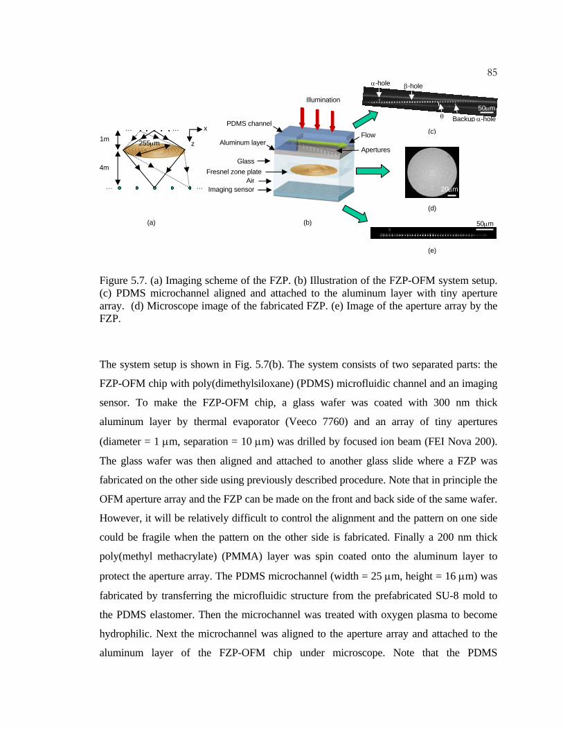
85
Figure 5.7. (a) Imaging scheme of the FZP. (b) Illustration of the FZP-OFM system setup. (c) PDMS microchannel aligned and attached to the aluminum layer with tiny aperture array. (d) Microscope image of the fabricated FZP. (e) Image of the aperture array by the FZP.
The system setup is shown in Fig. 5.7(b). The system consists of two separated parts: the
FZP-OFM chip with poly(dimethylsiloxane) (PDMS) microfluidic channel and an imaging
sensor. To make the FZP-OFM chip, a glass wafer was coated with 300 nm thick
aluminum layer by thermal evaporator (Veeco 7760) and an array of tiny apertures
(diameter = 1 μm, separation = 10 μm) was drilled by focused ion beam (FEI Nova 200).
The glass wafer was then aligned and attached to another glass slide where a FZP was
fabricated on the other side using previously described procedure. Note that in principle the
OFM aperture array and the FZP can be made on the front and back side of the same wafer.
However, it will be relatively difficult to control the alignment and the pattern on one side
could be fragile when the pattern on the other side is fabricated. Finally a 200 nm thick
poly(methyl methacrylate) (PMMA) layer was spin coated onto the aluminum layer to
protect the aperture array. The PDMS microchannel (width = 25 μm, height = 16 μm) was
fabricated by transferring the microfluidic structure from the prefabricated SU-8 mold to
the PDMS elastomer. Then the microchannel was treated with oxygen plasma to become
hydrophilic. Next the microchannel was aligned to the aperture array and attached to the
aluminum layer of the FZP-OFM chip under microscope. Note that the PDMS
PDMS channel
Flow
AperturesAluminum layer
GlassFresnel zone plate
Imaging sensor
Illumination
(b)
(d)
(c)
α-hole β-hole
Backup α-hole
20μm
50μm
Air
(e)
50μm
……
……
(a)
x
z1m
4m
255μm
θ

86microchannel can be peeled off after the experiment and a new PDMS microchannel can
be used with the same FZP-OFM chip for new experiment. The optical sensor (Lumenera
Lu-080M, with 9.9 μm pixel size) was located at the imaging plane of the FZP and the
aperture array was imaged by the FZP onto the sensor. The system was illuminated by an
elongated laser beam (~5 W/cm2) transformed by cylindrical lenses from a HeNe laser
(wavelength = 633 nm, Melles Griot 25-LHP-928-249) so that the power can be effectively
utilized. The optical system will be shown later. The different components of the system
are shown in Fig. 5.7(c)(d)(e).
Figure 5.7(c) shows the image of a PDMS microchannel attached to the aperture array. The
microchannel was oriented at a small angle θ = 3.3o with the aperture array. In the
experiment, the channel spanned 44 apertures. In addition to the aperture array, an α-hole
and a backup α-hole were drilled on the glass wafer with the same technique. The isolated
α-hole had the same size as other apertures and was positioned at the center of the
microchannel as shown in the figure. During the experiment, the α-hole and the
corresponding β-hole (distance between them is 170 μm) in the aperture array downstream
will scan the same part of the sample. By comparing the transmission from the α-hole and
the β-hole, we can monitor the flow stability and measure the flow speed. The correlation
of the transmissions through α, β-hole provides a good criterion for rejecting images of
unstable samples. Figure 5.8 shows an example of line scan signals acquired by the α, β-
hole. The flow speed V can be calculated by
τdV = , (5.11)
where d and τ are the distance and the travel time of the sample between the α, β-hole,
respectively.

87
Figure 5.8. Signals of α, β-hole.
Figure 5.9. Transmitted signal of the apertures in one line of the imaging sensor.
0 50 100 150 2000
50
100
150
200
Pixel index
Inte
nsity
(a.u
.)
0 200 4000
100
200
Time(ms)
Tran
smis
sion
(a.u
.)
α-hole
β-hole

88Figure 5.7(d) is a microscope image of the fabricated FZP. Figure 5.7(e) shows the
image of the aperture array projected by the FZP onto the optical sensor. We can see that
the transmission of all apertures, except those blocked by the edges of the microchannel,
were well projected and distinguishable from each other. Figure 5.9 shows the transmitted
signal of the apertures in one line of the imaging sensor. Note that the detected optical
power from different apertures varies and, as such, we need to normalize the power of the
apertures during data processing.
Figure 5.10. Inlet of the microfluidic channel.
Before the experiment, the surface of the channel was coated with Poly(ethylene glycol)
(PEG) to promote smooth microfluidic flow [16]. The process of coating PEG was to put a
drop of PEG solution into the microchannel and illuminate the channel by UV light for
5min, and then repeat the process three times. During the experiment, the channel was
oriented almost vertically to actuate microfluidic flow by gravity. The inlet of the channel
was designed to be a tunnel shape to facilitate the flowing of the sample into the channel, as
shown in Fig. 5.10. While the sample was flowing through the microfluidic channel, the
transmitted light of the aperture array was detected by the imaging sensor and each aperture
effectively acquired a line scan of the sample. Note that the exposure time of the imaging
sensor should be set appropriately so that when there is no sample, the pixel value is
roughly half of the maximum value. This is because the sample can attenuate the light
Flow direction
50 μm

89incident into the pixel by blocking part of the light, as well as strengthen the light by
focusing effect of certain part of the sample. Thus the exposure time can allow maximum
dynamic range during imaging.
L1
HeNeO1
CL1 CL2
FZP-OFMmodule
O2
Filter 1
BS Illumination
Imagingsensor
L2
Microscope module
Filter 2
L1
HeNeO1
CL1 CL2
FZP-OFMmodule
O2
Filter 1
BS Illumination
Imagingsensor
L2
Microscope module
Filter 2
Figure 5.11. Illumination for the FZP-OFM and the microscope module for monitoring. O1, O2: objective lens 1 and 2; L1, L2: lens 1 and 2; CL1, CL2: cylindrical lens 1 and 2; BS: beamsplitter.
The optical system besides the FZP-OFM module is shown in Fig. 5.11. The laser from the
HeNe laser was first expanded by objective lens 1 (magnification M = 10x) and lens 1
(focal length f = 100 mm), then compressed in one direction by two cylindrical lenses
(focal length f = 40 mm and f = 5.8 mm). The beam then became elongated and further
focused by objective lens 2 on the FZP-OFM chip. The microscope module (in the dotted
box) was added to monitor the experiment for convenience. The lens 2 and objective 2
imaged the microfluidic channel of FZP-OFM chip onto the imaging sensor. Filter 1 was
used to transmit red light (the HeNe laser) and reflect microscope illumination light so that
the HeNe laser will not be attenuated and the microscope illumination light can illuminate
the FZP-OFM chip. Filter 2 was inserted to filter out the residue backreflected red light
from the FZP-OFM chip because it was usually still strong enough to saturate the sensor.
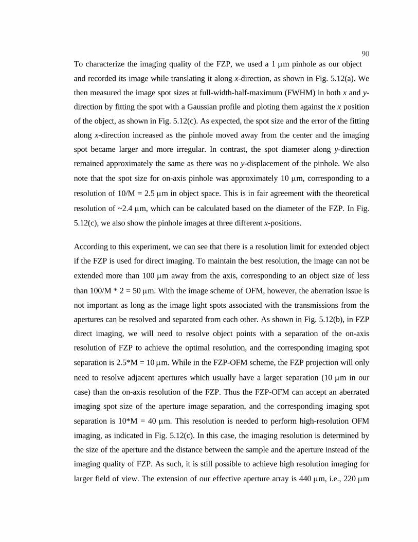
90To characterize the imaging quality of the FZP, we used a 1 μm pinhole as our object
and recorded its image while translating it along x-direction, as shown in Fig. 5.12(a). We
then measured the image spot sizes at full-width-half-maximum (FWHM) in both x and y-
direction by fitting the spot with a Gaussian profile and ploting them against the x position
of the object, as shown in Fig. 5.12(c). As expected, the spot size and the error of the fitting
along x-direction increased as the pinhole moved away from the center and the imaging
spot became larger and more irregular. In contrast, the spot diameter along y-direction
remained approximately the same as there was no y-displacement of the pinhole. We also
note that the spot size for on-axis pinhole was approximately 10 μm, corresponding to a
resolution of 10/M = 2.5 μm in object space. This is in fair agreement with the theoretical
resolution of ~2.4 μm, which can be calculated based on the diameter of the FZP. In Fig.
5.12(c), we also show the pinhole images at three different x-positions.
According to this experiment, we can see that there is a resolution limit for extended object
if the FZP is used for direct imaging. To maintain the best resolution, the image can not be
extended more than 100 μm away from the axis, corresponding to an object size of less
than 100/M * 2 = 50 μm. With the image scheme of OFM, however, the aberration issue is
not important as long as the image light spots associated with the transmissions from the
apertures can be resolved and separated from each other. As shown in Fig. 5.12(b), in FZP
direct imaging, we will need to resolve object points with a separation of the on-axis
resolution of FZP to achieve the optimal resolution, and the corresponding imaging spot
separation is 2.5*M = 10 μm. While in the FZP-OFM scheme, the FZP projection will only
need to resolve adjacent apertures which usually have a larger separation (10 μm in our
case) than the on-axis resolution of the FZP. Thus the FZP-OFM can accept an aberrated
imaging spot size of the aperture image separation, and the corresponding imaging spot
separation is 10*M = 40 μm. This resolution is needed to perform high-resolution OFM
imaging, as indicated in Fig. 5.12(c). In this case, the imaging resolution is determined by
the size of the aperture and the distance between the sample and the aperture instead of the
imaging quality of FZP. As such, it is still possible to achieve high resolution imaging for
larger field of view. The extension of our effective aperture array is 440 μm, i.e., 220 μm

91away from the axis, and is well within the capability of our FZP-OFM system. As
expected, the acquired OFM images shown in the next section is much better than the
images acquired by direct FZP imaging.
Figure 5.12. (a) Experimental scheme to characterize the imaging quality of the FZP; (b) Demonstration of resolution needed to perform FZP direct imaging and FZP-OFM imaging; (c) Measured FWHM spot size of the image in x- and y-direction versus the x- position of a 1 μm pinhole. Pinhole images in three different positions are shown. The resolution limit of the FZP and the resolution needed for the FZP-OFM imaging are indicated.
0 50 100 150 200 250 3000
10
20
30
40
50
60
70
x(μm)
FWH
M s
pot s
ize
( μm)
y-direction size
x-direction size
Resolution limit of the FZP
x
z
pinhole
Imaging sensor
Fresnel zone plate
Extension of the OFM aperture array
(b)
(c)
(a)
FZP Direct imaging
Resolution needed for our OFM scheme
FZP-OFM imaging
10 μm
40 μm

92Application in OFM Imaging
As a demonstration, we acquired images of the protist Euglena gracilis (Carolina Biology
Supply Company) with the FZP-OFM system. We immobilized the protists by treating
them in a 90oC heat bath for 15 second. The solution containing the protists was then
injected into the input port of the FZP-OFM system. By tilting the FZP-OFM vertically, we
were able to induce the solution to flow through the microfluidic channel. During the
imaging process, the flow speed of the protists was measured by the α, β-hole pair to be V
~ 400μm/second. The imaging sensor was operated at a frame rate of F = 1350 frames/sec.
The pixel spacing (or size) of the OFM images was δx = 0.3μm and δy = 0.6μm. The
acquisition time for the protists images was ~1 second.
Figure 5.13 is an image compilation of similar protists acquired with the FZP-OFM and
other imaging schemes. Figure 5.13(a) was acquired by simply using a FZP to directly
image a protist onto our optical sensor. We can see that the image is blurry and is
negatively impacted by the presence of a diffraction background. In comparison, the FZP-
OFM images shown in Fig. 5.13(b) are clearer and well resolved. Since our FZP-OFM
system used coherent laser as illumination, we believe that a comparison of the acquired
images to those from a conventional microscope operating with coherent illumination and
incoherent illumination would be helpful. Figure 5.13(c) and (d) show images of the protist
that are acquired with a microscope (Olympus BX41) through a 20x objective under
coherent and incoherent illumination, respectively.
It is interesting to note that the FZP-OFM images appear to be more similar to the
incoherent illumination conventional microscope image than the coherent illumination
conventional microscope image, despite the fact that FZP-OFM also employed a coherent
illumination source. The speckle background in Fig. 5.13(c) arose from the interference of
stray light components scattered and reflected from various interfaces in the microscope.
This pattern varied spatially but had no time varying component. The absence of this
speckle background in Fig. 5.13(d) is attributable to the washout of such interference effect
in incoherent illumination. The absence of the speckle background in our FZP-OFM
images can be explained by noting that each horizontal line in the images represents a time

93trace of an aperture in the array. In the absence of an object directly above the aperture,
we can expect the transmission through the aperture to remain unchanged in time. The
transmission through each aperture was normalized with respect to each other at the
beginning of the experiment. This was intended to correct for small variations in the
aperture size and sensor sensitivity. However, variations in light intensity incident on the
apertures would be, likewise, normalized by this process. As such, the impact of a speckle
background in the FZP-OFM was effectively eliminated. We further note that the effect of
mutual light interference from scatterings within the object should remain in our FZP-OFM
images.
Figure 5.13. Images of Euglena gracilis acquired by (a) FZP direct imaging; (b) FZP-OFM system; (c) conventional microscope with 20x objective under coherent illumination; (d) conventional microscope with 20x objective under incoherent illumination.
Figure 5.14 shows two more OFM images of a 10 μm microsphere (Fig. 5.14(a)) and a
chlamydomonas (Fig. 5.14(b)) acquired by the FZP-OFM system. Note that the center of
(b)
10μm
10μm
(a)
(d)
10μm 10μm
10μm
(c)

94the microsphere appears to be bright. This is because it acts as a ball lens and focuses the
illumination light.
Figure 5.14. (a) OFM images of a 10 μm microsphere; (b) OFM images of a chlamydomonas;
Figure 5.15. An example of OFM image of a rotating microsphere.
Note that the movement of spherical sample such as microsphere or chlamydomonas under
gravity driven flow might not be as smooth as the elongated sample such as Euglena.
Actually, they will tend to rotating in the channel and prevent successful OFM imaging.
Thus the probability of getting a good OFM image in this case is not high. For spherical
samples, the electroosmosis flow might be a better choice for better imaging [2]. Figure
5.15 shows an example of OFM image of microsphere under rotation acquired by our FZP-
OFM system.
In summary, we have shown the application of the FZP in the OFM imaging scheme. We
have explained the principles of OFM and FZP and showed that the aberrations associated
10 μm
10 μm
(a)
(b)
10 μm

95with FZP do not impact or limit the resolution of the FZP-OFM, which is limited
fundamentally by the size of apertures employed. The experimental setup and fabrication
procedures are also explained. To demonstrate its capability, the prototype FZP-OFM
imaging system was applied to acquire microscopic images of the protist Euglena gracilis.
As this scheme allows the separation of the OFM aperture array from the optical sensor
array, it is advantageous for a number of scenarios. Specifically, this design allows for
easier recycling of high-cost optical sensor array and it allows for the cooling of the optical
sensor with less risk of freezing shut the microfluidic channel.
References
1. X. Heng, D. Erickson, L. R. Baugh, Z. Yaqoob, P. W. Sternberg, D. Psaltis, and C. Yang, “Optofluidic microscopy – a method for implementing a high resolution optical microscope on an chip,” Lab on a chip 6, 1274-1276 (2006).
2. X. Cui, L. M. Lee, X. Heng, W. Zhong, P. W. Sternberg, D. Psaltis, and C. Yang, “Lensless high-resolution on-chip optofluidic microscopes for Caenorhabditis elegans and cell imaging,” Proceedings of the National Academy of Science 105, 10670-10675 (2008).
3. X. Heng, E. Hsiao, D. Psaltis, and C. Yang, “An optical tweezer actuated, nanoaperture-grid based optofluidic microscope implementation method,” Optics Express 15, 16367-16375 (2007).
4. G. M. Whitesides, “The origins and the future of microfluidics,” Nature 442, 368-373 (2006).
5. J. Wu, X. Cui, L. M. Lee, and C. Yang, “The application of Fresnel zone plate based projection in optofluidic microscopy,” Optics Express 16, 15595-15602 (2008).
6. D. Lange, C. W. Storment, C. A. Conley, and G. T.A. Kovacs, “A microfluidic shadow imaging system for the study of the nematode Caenorhabditis elegans in space,” Sensors and Actuators B 107, 904-914 (2005).
7. X. Heng, Optofluidic microscopy: technology development and its applications in biology, PhD thesis, California Institute of Technology (2008).
8. X. Heng, X. Cui, D. W. Knapp, J. Wu, Z. Yaqoob, E. J. McDowell, D. Psaltis, and C. Yang, “Characterization of light collection through a subwavelength aperture from a point source,” Optics Express 14, 10410 (2006).
9. X. Cui, X. Heng, J. Wu, Z. Yaqoob, A. Scherer, D. Psaltis, and C. Yang, “Slanted hole array beam profiler (SHArP) – a high-resolution portable beam profiler based on a linear aperture array,” Optics Letters 31, 3161-3163 (2006).
10. X. Cui, M. Lew, and C. Yang, “Quantitative differential interference contrast microscopy based on structure-aperture interference,” Applied Physics Letters 93, 091113 (2008).
11. A. G. Michette, Optical systems for soft X rays (Plenum Press, 1986), Chapter 8. 12. R. M. Henkelman and J. J. Bronskill, “Imaging extended objects with a Fresnel-zone-
plate aperture,” Journal of the Optical Society of America A 64, 134-137 (1974).

9613. M. Young, “Zone plates and their aberrations,” Journal of the Optical Society of
America A 62, 972-976 (1972). 14. F. Wyrowski, “Diffractive optical elements: iterative calculation of quantized, blazed
phase structures,” Journal of the Optical Society of America 7, 961-969 (1990). 15. A. R. Jones, “The focal properties of phase zone plates,” Journal of Physics D 2,
1789-1791 (1969). 16. S. W. Hu, X. Ren, M. Bachman, C. E. Sims, G. P. Li, and N. Allbritton, “Surface
modification of Poly(dimethylsiloxane) microfluidic devices by ultraviolet polymer grafting,” Analytical Chemistry 74, 4117-4123 (2002).

97C h a p t e r V I
CONCLUSION
Summary
Interferometers and coherence domain optical techniques play an important role in modern
biomedical research and applications. The research projects on imaging techniques that I
have done are explained in detail in this thesis and can be summarized as follows:
1) A forward-imaging probe for optical coherence tomography, PARS-OCT probe, was
built and tested by acquiring OCT images of a Xenopus laevis tadpole. The principles of
the OCT system and the PARS-OCT probe are explained. The prototype probe has an outer
diameter of 1.65 mm and can scan the beam over a wide angular arc (~19o half angle) of
the region forward of the probe. Under the working wavelength of 1300 nm, the working
distance and the focal spot size of the prototype probe are ~1.4 mm and ~10 μm,
respectively. One of the most important advantages of the PARS-OCT probe design is that
it can be readily miniaturized. Another important advantage of the probe is that it can scan
the whole 3D cone region ahead of the probe and be possibly used to acquire 3D OCT
images. The PARS-OCT probe can be potentially used in needle surgical procedures to
provide high-resolution 3D tomographic images of the targets forward of the probe.
2) The principle of the G1G2 interferometry, where a harmonically matched diffraction
grating (G1G2 grating) is used as a beam splitter/combiner in the interferometer setup, is
presented and explained. Using the G1G2 interferometry, we have built a proof-of-
principle experimental setup for measuring phase and intensity information of the sample
quantitatively. Phase images of standard phase object and diffusion process of microfluidic
mixing are acquired to demonstrate the capability of the system. The technique of G1G2
interferometry has many advantages. First, the optical setup and the data processing to
extract phase and amplitude information are both relatively simple and easy to implement.
Second, the principle can be adapted to other wavelengths such as x-ray or terahertz. Third,

98the G1G2 grating is a planar device and can be directly fabricated into a layered
microstructure easily. This can possibly lead to a compact and low-cost device. Finally, the
imaging speed is limited only by the speed of the camera and thus the technique can be
used to observe fast dynamics of biological samples.
3) An improved version of full-field phase-imaging system based on the G1G2
interferometry is presented and explained. Compared with the previous proof-of-principle
setup, the improved version features improvement in optical setup, where the aberration
caused by grating diffraction is removed, and in data processing, where the requirement of
relative power of reference and sample beams are much less restricted. The two major
improvements are explained in detail. Then the phase noise of the system is theoretically
analyzed and experimentally calibrated. The phase stability is measured to be 62 mrad,
corresponding to 6.24 nm optical path length. The improved system is used to observe
biological samples that have many details, such as onion. And it is also used to observe the
movement of an amoeba proteus. The imaging results show that the phase image can
provide much better contrast than the intensity image especially for transparent biological
samples. And because of its fast imaging speed, our technique can be readily used to
observe fast dynamics of the sample.
4) Optofluidic microscopy (OFM) is a novel high-resolution lensless on-chip compact
microscopy technique developed by our group. In this thesis, the application of the Fresnel
zone plate (FZP) in OFM is explained and demonstrated. The FZP is used to project the
images of the OFM aperture array onto the imaging sensor such that the imaging sensor can
be separated from the OFM aperture array. The separation is important for some situations.
One of the situations is when we want to recycle the imaging sensor especially if the sensor
is expensive. The separation will thus reduce the cost of the system. Another situation is
when we want to cool the imaging sensor to provide better sensitivity. In this case, the
separation scheme can ensure that the cooling will not affect the biological sample that is
under observation. The FZP-OFM system is used to acquire OFM images of 10 μm
microsphere, chlamydomonas, and the protist Euglena gracilis. The imaging results also

99show that although the system use a coherent laser for illumination, the speckle effect of
the laser is not apparent. The phenomenon is explained in this thesis.
Future Studies
The coherence domain optical imaging techniques and the novel ideas shown in my thesis
might have possible improvement and applications. Here I want to present some related
possible future studies. And I believe at least some of them should be possible to
implement.
1) To implement 3D OCT imaging using the PARS-OCT probe. In principle, the PARS-
OCT probe can be used to scan the whole 3D cone region forward of the probe. In our
preliminary study, the two GRIN lens are counter rotated to acquire only a B-scan image.
Although this can clearly demonstrate the capability of the PARS-OCT probe compared
with other endoscopic OCT probes, the PARS-OCT probe can be more powerful.
The difficulties associating with the 3D imaging can be summarized as follows. First, the
scanning pattern of the probe must be carefully chosen and characterized, including exact
position, and nonlinear scan compensation, etc. Second, the forward scanning is generally
nonlinear and might results in oversampling and undersampling of different part of the
sample. This needs to be considered in the final display of the image. Third, the
reconstruction and rendering of the 3D image is not straightforward. The 3D scan pattern of
the PARS-OCT probe might be complicated and the register of the A-scan lines will need
to be handled carefully.
Despites the above difficulties, in some applications the 3D image might be very helpful
and it should be worth pursuing for the PARS-OCT probe.
2) To build a robust miniature PARS-OCT probe for biomedical application. My
colleagues have built a miniature PARS-OCT probe with diameter of 820 μm. It might be
still possible to build smaller probe. And the design of the probe and the actuation system
can be possibly improved to make it robust enough for practical biomedical applications.
This is actually the ultimate goal for developing the PARS-OCT probe.

1003) Development of compact on-chip phase imaging system based on the principle of the
G1G2 grating. The G1G2 grating is a planar device and can be made on-chip using current
microfabrication techniques. It might be possible to utilize the unique characteristics of the
G1G2 grating to build an on-chip phase imaging system. Diffractive optical element such
as the Fresnel zone plate might also be possibly used in the system.
4) Application of the FZP on other variations of OFM, such as illumination type OFM, grid
based OFM. The use of FZP can separate the imaging sensor from the OFM chip and is
useful for some situations.