coding/decoding for data compression and error control … · coding/decoding for data compression...

Coding/decoding for data compression and error control on data links using digital computers

by H. lV1. GATES

Braddock, Dunn and McDonald, Inc. Albuquerque, New Mexico

and

R. B. BLIZARD

Martin Marietta Corporation Denver, Colorado

INTRODUCTION

Data compression and error control have, over the years, been treated as two separate disciplines. Data compression can substantially reduce the loading of communication channels and error control using coding methodology, can reduce the amount of errors in the messages being transmitted, or allow the· system to operate with less power for a comparable uncoded information rate. This paper demonstrates that both functions can be combined into one operation by applying sequential decoding developed for error control to data compression. Because the same general method can be used to solve both problems, data compression and error control can be united in a single system and held accountable for the required theorems in information theory.

The principal incentive for the use of sequential decoding for both compression and error control is that it permits the use of the source redundancy with extremely simple encoding equipment. Higher speed computing systems and larger available memories make it more feasible to use various redundancy schemes. In photographs, for example, line-to-line redundancy can successfully be used.

The proposed process of combining data compression and error control in a sequential decoder is reversible because the original data is recovered intact with no compromising or loss of information and resolution. This is attributed to the sequential decoding process itself. Uncertainty about data modification and missing data does not exist. If the capacity of the channel is exceeded because of increased noise or information activity beyond the design of the system, the data out-

503

put from the decoding process stops and delivers no further information until the channel improves. The transmitted data delivered to the user is thus creditable.

The combined process does not require two separate systems; one for compression and one for error control. Data compression designers rely heavily on error free channels and error control factions assume purely random information into their system and data link. Naturally, neither is completely true.

In simulating data channels, error control designers expend a great amount of effort in generating a pure random number sequence to test their system. Yet, the data compression specialist expends his time trying to identify patterns in what is sometimes the most obscure material. There should be little doubt that the two· processes are very closely related.

Background

The means for decoding convolutional codes first became practical when R. M. Fano in 1963 introduced his now famous sequential decoding algorithm. 1 ,2 1. M. Ja'cobs3 recently discussed sequential decoding as it applies to retrieving data from a space probe. He points out that this is a particularly good application because fading is relatively unimportant, channel noise is nearly Gaussian, and the information rate is limited by the available signal strength rather than by the bandwidth. Significant developments in the im.plementation of sequential decoders have occurred in the Pioneer IX space program;4 at the MIT Lincoln Laboratory;5 and by the Codex Corporation;6 and new algorithms for decoding convolutional codes are being disclosed annually.7

From the collection of the Computer History Museum (www.computerhistory.org)

504 Fall Joint Computer Conference, 1970

n = I k = It v 2 3

(

1000 ) G = 1111

1011

move is up if m .. 0

n

move is down if m .. I

n

Noise'

(a) Convolutional Encoder

n+3

(b) Code. Tree

H=O,I,O,O

Figure l-Binary convolutional encoder and its code tree for first 4 moves

The possibility of applying error control coding to data compression was first pointed out by Weiss8 who showed that block codes work fairly well for compressing data streams consisting of a few l's scattered at random among many O's. However, this type of source can be very efficiently and easily encoded with a run-length encoder. More interesting sources are those in which the redundancy is of a more complicated type and is not easily utilized by a block decoder. Sequential decoding is ideally suited to this type of problem.

With block codes such as the orthogonal and BCH codes, the entire block is ordinarily decoded as a unit by computing correlations or by solving certain alge~ braic equations. Sequential decoding starts at the beginning of a message block and works toward the end by a trial-and-error process. A running account is kept of the reasonableness of the decoded message on the basis of received signal. If a wrong decision is made because of noise, the subsequent decoded message soon becomes unreasonable, and the decoder then searches back over its earlier choices until the correct message is found. It is relatively simple, in concept at least, to use what is known about the message probabilities to improve the likelihood criterion. This aUows more data to be tr~nsmitted over a given link and accomplishes data compression.

Convolutional Codes

Figure la shows a convolutional encoder with a binary message source, M, assumed for the time being to be random information, and an error source, N, representing channel noise. Messages from the source S may be shifted in one or more bits at a time denoted as n. After each shift, v mod-2 adders (in this case three mod-2 adders) are sampled or commutated and the resultant bits passed into the transmitter equipment of the data channel. If four bits are shifted in before the encoder output is commutated, a convolutional data compression process occurs at rate %. The decoder must then use the a posteriori probability of the source S in defining the decoding parameters of the Fano algorithm. Normally, rates of Y2, ~, and even 7.4: are used in error control. That is, for each bit shift in, from two to four mod-2 adders are sampled. The number of mod-2 adders normally is fixed or hardwired for a particular mission or channel requirement. The connections from these mod-2 adders to the shift register, G, represents the codes themselves and a great deal has been written about this subject particularly if the shift register length, called the constraint length, k, is below 12 to 15 bits. Random selection of these codes for large constraint lengths produces adequate, if not complete1y satisfactory, results.9 Two rates of 2/1 and 6/4 are demonstrated here. Constraint lengths of 60 bits are used as well.

The basic channel

The channel is important in both error control and compression since it represents the sole source of noise and thus errors into the system, that is, receiver frontend noise, electronic noise in the lines, and so forth, are combined into one noise error source. By definition then, the channel referred to here contains the system modulator, amplifiers, transmitters, antennas or cables, repeaters, receivers, and demodulators. The noise of this channel is assumed to be Gaussian or white noise. The channel is assumed to be stationary in the sense that its properties do not change with time. And the channel· is assumed to be memoryless. The channel is described as binary antipodal in which the transmitted waveforms in the absence of noise are a sequence of 180 degree, phase-modulated waveforms, or binary data represented by plus and minus voltages for ones and zeros respectively.

The restrictions imposed on the channel are to this point, fairly realistic, depending of course on the method of transmission. In passing, if the received


Coding/Decoding for Data Compression and Error Control 505

binary sequence is quantized into say four or eight levels for each bit received, the compression and error control performance can be increased. This is a well known fact in information theory. This quantization does not change the basic operation of this system or any of the convolutional decoders that this author is aware of.

The decoder

Convolutional codes generated by the encoder shown in Figure 1a can be decoded in one of several ways. The oldest practical method is the use of the Fano Algorithm which is well described in several references. 2 The Fano Algorithm sequentially decodes the data stream as it is received and thus the reference to sequential decoding. Actually, there are several new algorithms for decoding convolutional codes which are extremely clever and add promise to the combination of error control and data compression.

Without going into great detail, a sequential decoding process will be described next. Any code produced by the convolutional encoder may be represented by a binary tree. The encoder input M =Ml, M 2, ••• , corresponds to an infinite path through the tree, and labels on the branches indicate the encoder output. Figure 1 b demonstrates this point for a given convolutional encoder. Since more bits are being generated than received in the. encoder, i.e., n<v, redundancy is introduced to give the code error detecting and correcting capabilities. The received infinite sequence for the channel must similarly be compared with a receiver encoder replica to find the path which maximizes the conditional probability of the received sequence versus the absolute values of the code tree. Each move from one node to another represents a bit shift of information. Sequential decoding is then based on searching the most probable branches of a code tree. Whenever this path becomes too unlikely, a search is initiated for a better path. The sequential decoder is able to determine the correct path while examining only a fraction of the total set of possible paths. The number of searches depends on the errors introduced by the channel in the case of error control. If the channel is very noisy, the number of branches which must be searched before finding the most probable path becomes super exponential. The decoder is limited by the operating speed of the computer and the decoder input rate. The means of scoring which branch or path is best is referred to as the branch metric which is based on the conditional probabilities of the received versus the transmitted signal.

THE COMPUTATIONAL LIMIT

This section contains a discussion of the limits of performance that can be expected for data compression with sequential decoding.

If the convolutional code is fairly long, a sequential decoder has a very small probability of making an undetected error. Instead, when the signal-to-noise ratio gets too high, it runs out of computational capacity and gives up until a new block is started by filling the encoder shift register with zeros. The amount of computation required for each node of the decoding tree is measured by the average number of branches that must be tried before the decoder can advance to the next node. It is easily seen that, as the signal gets noisier (or, if compression is used, as the data become more active), the decoder will make the wrong choice more often, and more trials must be made before the right path is found.

At a certain point, called the computational limit, the average number of trials per node becomes infinite, and the decoder is bound to break down at least .occasionally. Work can progress beyond this limit if some losses in the message can be accepted-e.g., when it is possible to obtain a repetition of the parts that were lost. In general, however, the computational limit is a good criterion for the capacity of a channel using sequential decoding. Operation is very good to within a few percent of the limit, and is poor when the limit is exceeded.

The computational limit is also equal to the union bound on the exponential error parameter for block coding.Io Consider a code block that contains N successive transmitted signals. These may be biphase pulses, or they may be the tones of a frequency-shift-keying transmitter or any other discrete modulation scheme. This code block will be used to convey the information contained in N' successive message symbols. These may be the gray levels of N' picture elements, or perhaps N' letters of English text. It will be shown that there are codes (i.e., rules for mapping the N' symbols into the N signal elements) for which the probability of one or more errors in the block P e is bounded by

P e5: 2-NEo (p , Q)+N' D(p) (1)

where E (p, Q) is a function of the signal-to-noise ratio in the channel and D (p) depends on the message statistics. It is convenient to define R' = N' / N as the decoding rate. Equation. (1) can be rewritten as

(2)

to show that fora fixed R', the probability of error decreases exponentially with increasing N so long as R'D(p) <Eo(p, Q). This defines the limiting rate Rc=



Eo(p, Q) /D(p) that is also the computational limit for sequential decoders.

The proof of Equations (1) and (2) can be shown using Gallager'S joint source and channel coding theorem.9 Gallager leaves the proof of a maximum a posteriori probability decoder r:equired for this system to the reader in problem 5.16 which I should like to do as well, although a complete proof does exist on request.u The results of Gallager's joint source and channel coding theorem for a discrete memoryless channel with equiprobable symbols is

Pe~2-N{ Eo(p,Q)+pR}

as opposed to the extended results of Equations (1) and (2) above. The units of Eo(p, Q) are in bits/ channel symbol. The equivalence between Rand R'D (p) exists so their units are the same. The ratio R' has units of data symbols/channel symbol and D(p) in bits/ data symbol. This agrees with pR so p is not dimensional and R is in bits/channel symbol. The term pR may in this case be interpreted as entropy since the binary source digits are independent and equiprobable. Although R'D (p) is not, in itself, entropy, it serves as a means of measuring system performance given the ideal case of pRo

Because Eo(p, Q) is determined by the communication link itself, exclusive of encoders and decoders, D is the quantity that determines how much a given message can. be compressed. If p = 1

(3)

where the { Wi} are the probabilities, based on all knowledge available to the decoder, of the possible message symbols. For instance, if the message is English text, each Wi would be the probability that the next symbol is a particular . letter or punctuation mark. The decoder could be programmed to take into account the part of the message already decoded, word frequencies, and the idiosyncrasies of the particular writer.

D is the number of bits that would have to be transmitted on an errorless channel to convey the information in each message symbol. . In the following sections, D will be evaluated for various types of source statistics.

Equiprobable symbols

Evaluating D in Equation (3) is particularly simple when all the symbol probabilities are the same. For the binary case, Wo = Wl= Y2and D = 1, indicating that the units of D are bits.

With m equiprobable symbols, Wi = l/m for i = 1, 2, 3, ~ .. m, and D = log2 m. This is exactly equal to the

entropy H for this case and indicates that the computational limit is the same as the Shannon bound for discrete noiseless systems. Of course, this is not a very interesting kind of source for data compression, but if m =3, for instance, the message could be coded into about 1.6 bits/symbol instead of going to 2 bits as would be required for a strictly binary system. Blizard, et al.,ll have shown interesting values for D based on some common distributions several of which are given in this paper.

Binary source with unequal probabilities

A binary source emits only two different symbols. These may be called one and zero. If the probability of one symbol is greater than that of the other, the data stream can be compressed.

If the probability of one symbol isp, and that of the other I-p, Equation (3) becomes

D = log2 [(p )1/2 + (1-P )1/2J2

= log2 {1 +2[p(I-p) JI/2}.

The corresponding expression for the entropy is

- H = P log2 P + (I - p) log2 (1- p) .

Figure 2 shows the amount of .compression, in, dB, that can be accomplished with sequential decoding and also the theoretical limit based on the entropy H. It is seen that sequential decoding will give slightly more than half the available improvement measured in dB.

A line drawing is an example of a binary source. In this case, there is a large amount of redundancy in the two-dimensional picture that is available by extrapo-

o

~ 3 o '':; 4 IV a:

omputat ional l imi t/

./ ,/

./ ,/ /

~ :::: ~'""" ",,/ V

/ /

/ L Entropy

c: 5 ,~ O/l

~ 6 / L Q. E

.3 7

10 0,01

/ /

/V

Ji/ 0.02 0,04 0,06 0, I 0.2 0.4 0.6

Ratio of Symbol Probabilities, p/(J-p)

Figure 2-Compression limits for a binary source

1.0



6

5 r- Note:

it

Normal Distribution, quantum

~ interval - 1.0, standard / deviation - C1 -III ...,

..0 -0 3 "'0 C co

:J: 2

~ /

/

~ /" lJI~ ~

~ ~II~

-~ ~ ~~

~

~ Ai ~

V'" ~~rrerl BTdS

~ o o. 1 0.2 0.5 1.0 2.0 5.0

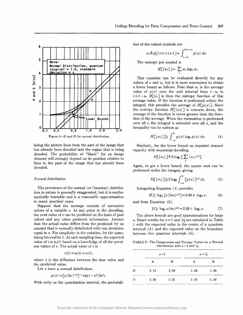
Figure 3-H and D for normal distribution

lating the picture lines from the part of the image that has already been decoded into the region that is being decoded. The probability of "black" for an image element will strongly depend on its position relative to lines in the part of the image that has already been decoded.

Normal distribution

The prevalence of the normal (or Gaussian) distribution in nature is generally exaggerated, but it is mathematically tractable and is a reasonable approximation in many practical cases.

Suppose that the message consists of successive values of a variable v. At any point in the decoding, the next value of v can be predicted on the basis of past values and any other pertinent information. Assume that the actual value· differs from the predicted by an amount that is normally distributed with rms deviation equal to u. For simplicity in the notation, let the quantizing interval be 1. At each sampling time, the expected value of v is vo(t) based on a knowledge of all the previous values of v. The actual value of v is

v(t) = vo(t) +x(t),

where x is the difference between the true value and the predicted value.

Let x have a normal distribution:

p (x)= [u(27r) 1/2J-1 exp ( - x2/2(2).

With unity as the quantization interval, the probabili-

ties of the output symbols are

jl+1-VO

wi!:p[i<v<i+IJ=. p(x) dx. ~-vo

The entropy per symbol is

H[{Wi} J = L: Wi log2 Wi· i

This equation can be evaluated directly for any values of (J and Vo, but it is more convenient to obtain a lower bound as follows. Note that Wi is the average value of p (x) over the unit interval from i - Vo to i+ I-vo. H[WiJ is then the entropy function of this average value. If the function is performed within the integral, this provides the average of H[p(x)], Since the entropy function H[ {wd J is concave down, the average of the function is never greater than the function of the average. When the summation is performed over all i, the integral is extended over all x, and the inequality can be written as

H[{wdJ~ f«> p(x) log2P(x) dx. -00

(4)

Similarly, for the lower bound on required channel capacity with sequential decoding,

D[ {wd J!: 2log2 [L (Wi)1/2]. i

Again, to get a lower bound, the square root can be performed under the integral, giving

D[{wdJ~2Iog2 foo [p(x)J/2dx. -00

(5)

Integrating Equation (4) provides

H~ log2 [u(27re)1/2J=2.05+ log2 u; (6)

and from Equation (5),

D~ log2 u(87r)1/2=2.33+ log2 u. (7)

The above bounds are good approximations for large u. Exact results for u = 1 and Y2 are tabulated in Table 1 with the expected value in the center of a quantum interval (A) and the expected value on the boundary between two quantum intervals (b).

TABLE I-The Compression and Entropy Values for a Normal Distribution with U' = 1 and Yz

U'=1 9'= Yz ----------

A B A B

H 2.11 2.09 1.24 1.36

D 2.38 2.37 1.43 1.50


508 Fall Joint Computer Conferen~e, 1970

Search and

110 - 2.32

60-bit word lengths

Source Encoder Decoder

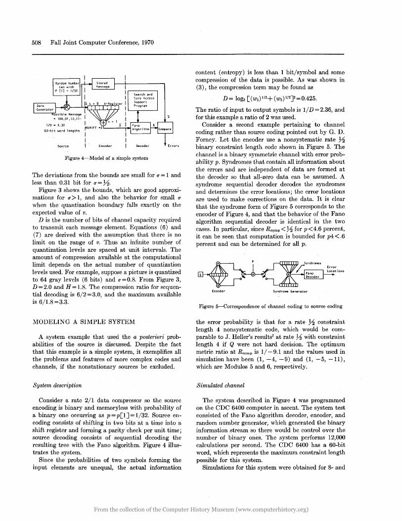
Figure 4-Model of a simple system

The deviations from the bounds are small for u = 1 and less than 0.31 bit for u = Y2.

Figure 3 shows the bounds, which are good approximations for u> 1, and also the behavior for small u when the quantization boundary falls exactly on the expected value of v.

D is the number of bits of channel capacity required to transmit each message element. Equations (6) and (7) are derived with the assumption that there is no limit on the range of v. Thus an infinite number of quantization levels are spaced at unit intervals. The amount of compression available at the computational limit depends on the actual number of quantization levels used. For example, suppose a picture is quantized to 64 gray levels (6 bits) and u=0.8. From Figure 3, D = 2.0 and H = 1.8. The compression ratio for sequential decoding is 6/2 =3.0, and the maximum available is 6/1.8 =3.3.

MODELING A SIMPLE SYSTEM

A system example that used the a posteriori probabilities of the source is discussed. Despite the fact that this example is a simple system, it exemplifies all the problems and features of more complex codes and channels, if the nonstationary sources be excluded.

System description

Consider a rate 2/1 data compressor sO the source encoding is binary and memoryless with probability of a binary one occurring as p=p[IJ=I/32. Source encoding consists of shifting in two bits at a time into a shift register and forming a parity check per unit time; source decoding consists of sequential decoding the resulting tree with the Fano algorithm. Figure 4 illustrates the system.

Since the probabilities of two symbols forming the input elements are unequal, the actual information

content (entropy) is less than 1 bit/symbol and some compression of the data is possible. As was shown in (3), the compression term may be found as

D = log2 [( wl)1/2+ (w2)1/2J2 = 0.425.

The ratio of input to output symbols is 1/ D = 2.36, and for'this example a ratio of 2 was used.

Consider a second examp] e pertaining to channel coding rather than source coding pointed out by G. D. Forney. Let the encoder use a nonsystematic rate Y2 binary constraint length. code shown in Figure 5. The channel is a binary symmetric channel with error probability p. Syndromes that contain all information about the errors and are independent of data are formed at the decoder so that all-zero data can be assumed. A syndrome sequential decoder decodes the syndromes and determines the error locations; the error locations are used to make corrections on the data. It is clear that the syndrome form of Figure 5 corresponds to the encoder of Figure 4, and that the behavior of the Fano algorithm sequential decoder is identical in the two cases. In particular, since Rcomp<Y2 for p<4.6 percent, it can be seen that computation is bounded for p4 < .6 percent and can be determined for all p.

Encoder Syndrome Generator

Figure 5~Correspondence of channel coding to source coding

the error probability is that for a rate Y2 constraint length 4 nonsystematic code, which would be comparable to J. Heller's results7 at rate 73 with constraint length 4 if Q were not hard decision. The optimum metric ratio at Rcomp is 1/ -9.1 and the values used in simulation have been (1, -4, -9) and (1, -5, -11), which are Modulos 5 and 6, respectively.

Simulated channel

The system described in Figure 4 was programmed on the CDC 6400 computer in ascent. The system test consisted of the Fano algorithm decoder, encoder, and random number generator, which generated the binary information stream' so there would be control over the number of binary ones. The system performs 12,000 calculations. per second. The CDC 6400 has a 60-bit word, which represents the maximum constraint length possible for this system.

Simulations for this system were obtained for 8- and



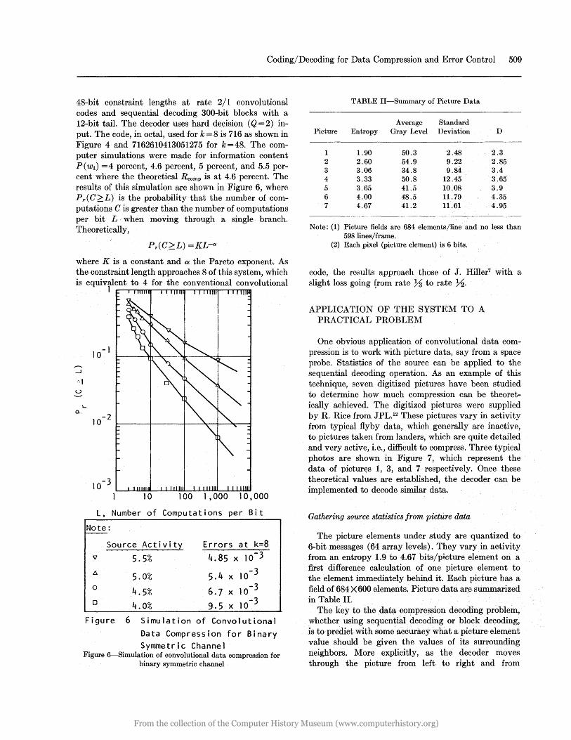
48-bit constraint lengths at rate 2/1 convolutional codes and sequential decoding 300-bit blocks with a 12-bit tail. The.decoder uses hard decision (Q=2) input. The code, in octal, used for k = 8 is 716 as shown in Figure 4 and 7162610413051275 for k=48. The computer simulations were made for information content P (WI) = 4 percent, 4.6 percent, 5 percent, and 5.5 percent where the theoretical Rcomp is at 4.6 percent. The results of this simulation are shown in Figure 6, where Pr(C?L) is the probability that the number of computations C is greater than the number of computations per bit L·· when moving through a single . branch. Theoretically,

Pr(C?L) =KL-a

where K is a constant and a the Pareto exponent. As the constraint length approaches 8 of this system, which is equivalent to 4 for the conventional convolutional

1

10- 1

....J

,',1 u

l-a..

10- 2

10 100 1,000 10,000

L, Number of Computations per Bit

Note:

Source Activity

~ 5.5%

o

o

5.0% 4.5% 4.0%

Errors at k=8

4.85 x 10-3

5.4 x 10-3

6.7 x 10-3

9.5 x 10-3

Figure 6 Simulation of Convolutional Data Compression for Binary Symmetri c Channe 1

Figure 6-Simulation of convolutional data compression for binary symmetric channel

TABLE II-Summary of Picture Data

Average Standard Picture Entropy Gray Level Deviation D

1 1.90 50.3 2.48 2.3 2 2.60 54.9 9.22 2.85 3 3.06 34.8 9.84 3.4 4 3.33 50.8 12.45 3.65 5 3.65 41.5 10.08 3.9 6 4.00 48.5 11.79 4.35 7 4.67 41.2 11.61 4.95

Note: (1) Picture fields are 684 elements/line and no less than 598 lines/frame.

(2) Each pixel (picture element) is 6 bits.

code, the results approach those of J. Hiller7 with a slight loss going ~rom rate ~ to rate Y2.

APPLICATION OF THE SYSTEl\1 TO A PRACTICAL PROBLEM

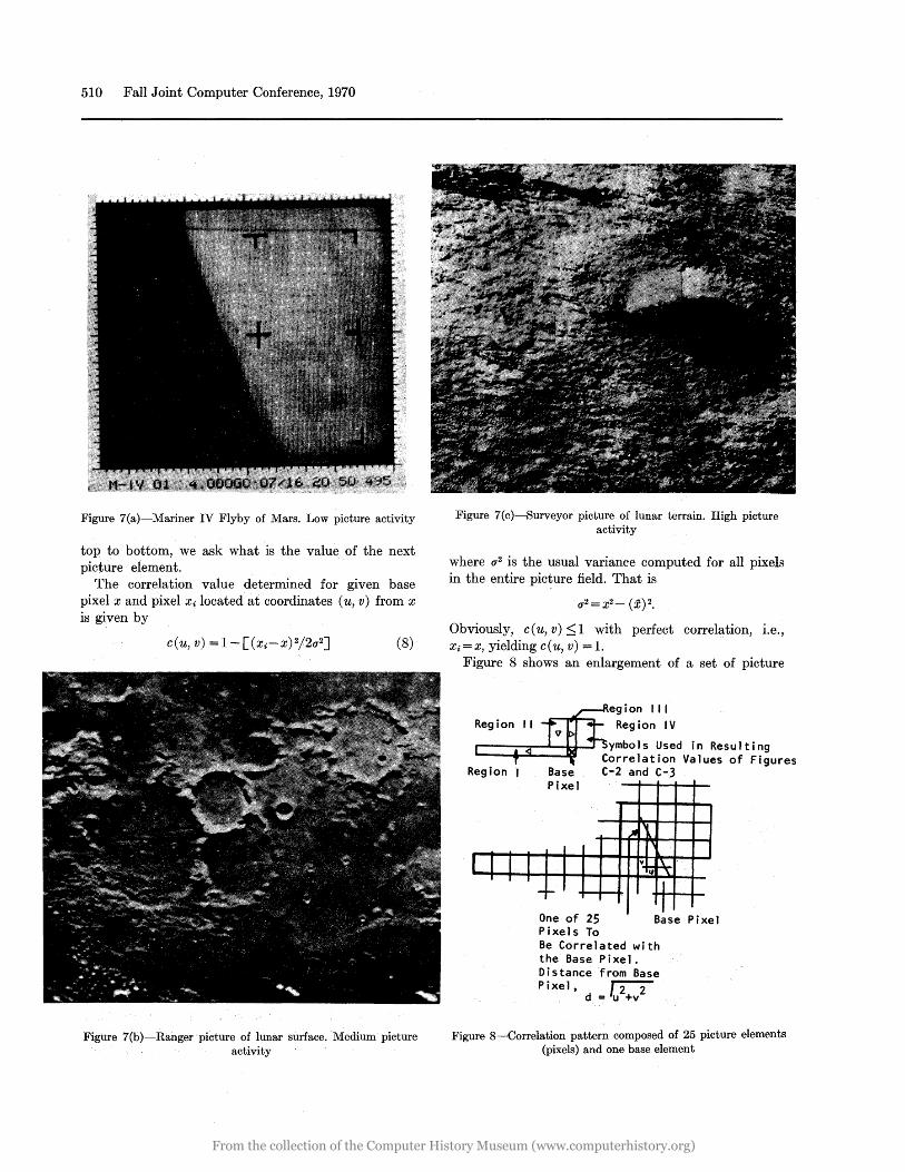
One obvious application of convolutional data compression is to work with picture data, say from a space probe. Statistics of the source can be applied to the sequential decoding operation. As an example of this technique, seven digitized pictures have been studied to determine how much compression can be theoretically achieved. The digitized pictures were supplied by R. Rice from JPL.12 These pictures vary in activity from typical fiyby data, which generally are inactive, to pictures taken from landers, which are quite detailed and very active, i.e., difficult to compress. Three typical photos are shown in. Figure 7, which represent the data of pictures 1, 3, and 7 respectively. Once these theoretical values are established, the decoder can be implemented to decode similar data.

Gathering source statistics from picture data

The picture elements under study are quantized to 6-bit messages (64 array levels). They vary in activity from an entropy 1.9 to 4.67 bits/picture element on a first difference calculation of one picture element to the element immediately behind it. Each picture has a field of 684 X 600 elements. Picture data.are summarized in Table II.

The key to the data compression decoding problem, whether using sequential decoding or block decoding, is to predict with some' accuracy what a picture element value should be given the values of its surrounding neighbors. More explicitly, as the decoder moves through the picture from left to right and from



Figure 7(a)-Mariner IV Flyby of Mars. Low picture activity

top to bottom, we ask what is the value of the next picture element.

The correlation value determined for given base pixel x and pixel Xi located at coordinates (u, v) from x is given by

(8)

Figure 7(b)-Ranger picture of lunar surface. Medium picture activity

Figure 7{c)-Surveyor picture of lunar terrain. High picture activity

where 0-2 is the usual variance computed for all pixels in the entire picture field. That is

0-2=X2- (X)2.

Obviously, c(u, v):::;l with perfect correlation, i.e., Xi=X, yielding c(u, v) = 1.

Figure 8 shows an enlargement of a set of picture

Region II

Region i

r I I I IT I

Base Pixel

--

egion II I Region IV

ymbols Used in Resulting Correlation Values of Figures C-2 and C-3

,A , I~; ~

J I

One of 25 Base Pixel Pixels To Be Correlated with the Base Pixel. Distance from Base Pixel, rr::;-

d = u +v

Figure 8-Correlation pattern composed of 25 picture elements (pixels) and one base element



elements. The x base pixel is correlated with each of the Xi elements within the pattern shown in the figure. When considering a pattern of more than one element, such as Figure 8, correlation becomes a function of distance, u and v, between the two pixels being correlated, where u is the horizontal distance and v the vertical distance. For the correlation pattern shown in Figure 8, 25 correlation values will be bound for one base pixel as a function of u and v.

After completing the 25 calculations, the base pixel is moved one unit to the right along the picture line and 2~ more correlation coefficients are recomputed. These new results are averaged into the past results. Once the correlation calculations have been computed for one line, the base pixel is moved down by one line and the data again computed and averaged with all the

en :I: I-:z UJ I-

:z

>

2-:z 0

I-~ ~ UJ a:: a:: 0 u

en o :z ~ en ~ o :I: I-

:z

10

20

18

16

14

12

10

8

6

4

2

2 3 4 5 6 7 8 9 10

SQUARE ROOT OF (U**2+V**2) CORRELAT10N FUNCTION

PIX 1 LOWER LEFT CORNER

4 81216 202428 3236 404448525660 64

GRAY LEVELS PROBABILITY DENSITY FUNCTION OF DATA SOURCE

PIX , LOWER LEFT CORNER

Figure 9-Autocorrelation of picture data using the pattern of Figure 8 (Probability density functions of the areas examined

are included)

10

- 9 en :I:

8 I-:z UJ I- 7 :z

6 >

2- 5

:z 4 0

I- 3 ~ ~ UJ 2 a:: a:: 0 u

-;;; 20 0

z ~ en 18 ~ 0 :z: 16 I-

:z 14

en UJ

12 ~ ~ 10 ~ > u 8 ~ 6 en 0 ~

UJ 4 > I- 2 ~ ~ ~ ~ ~ u

~<l

X

~i

2

~~ <I

<l <l

<l <l

3 4 5 6 7 8

SQUARE ROOT OF (u**2+V~b't2)

CORRELATION FUNCTION

PIX 4 UPPER RIGHT CORNER

<l

9

4 8 12 16 20 242832 36 40 4448 52 5660 64

GRAY LEVELS PROBABI LI TV DENSHY FUNCTION OF DATA SOURCE

PIX 4 UPPER RIGHT CORNER

<l

10

Figure lO-Autocorrelation of picture data using the pattern of Figure 8 (Probability density functions of the areas examined

are included)

previous work. This procedure was accomplished on a CDC 6400 digital computer.

The correlation pattern was subdivided, into. foul' regions, as indicated in Figure 8, to investigate directional variation. Samples of the results· of our correlation computations are shown in Figures 9 and 10 for two pictures. Each of the four symbols represents one of the four regions. The probability density functions are also shown for regions in which correlation data were established.

If the analyst wants to apply the correlation data to an· efficient prediction program, he must evaluate the results of Figure 8 using a mean square estimatiop. technique to determine how effective the correlation coefficients are in predicting results as a function of various patterns. The correlation patterns must be selected on the basis of which appears to be the most



0.7

q.6

rfh rR, rrr I I I I

~ ~ ~

1\ 5 6 9

............

c: ttJ (l,) 0.5 ~

E 0 '-4- 0.4 \ c: 0

+J ttJ ~ --> 0.3 (l,)

0

V')

~ 0.2 0::: ~ ............... ~

O. 1

o 2 3 4 5 ('v 6 9

Number of Elements Figure ll-RMS deviation from mean given a set of patterns

efficient. The pattern shown in Figure 8 was used to gather data rather than trying to determine an efficient pattern. These results are then applied to the sequential decoder algorithm.

Eleven pixel patterns were tested. These patterns, along with their performance, are shown in Figure II. The base pixel to be predicted is noted with an X.

The vertical axis of this figure is the rms deviation from the mean of the base pixel to the surrounding values. High rms deviations represent large. errors in estimating the base pixel values. The horizontal axis represents the number of elements used to evaluate the gray levels of the base pixels. The correlation coefficients were used for low, average, and highly correlated pictures. Thus, the top curve represents the rms deviation from mean for low correlated pictures using the different pattern structures shown. The middle curve and the bottom curve represent the average and highly correlated rms deviations from mean, respectively.

From this set of curves, it can be seen that after

four or five picture elements there is little need for the additional data supplied by more picture elements to estimate the value of the base picture element.

Extending the model

The example of the preceding section may he extended to handle the picture data discussttd here. Knowledge of the picture statistics aids in the deCoding process just as it did for the binary case. The only difference in the source is the complexity of the data . For this simulation, use was made of the statistics associated with Picture 2 (Table II), which are highly correlated. The standard deviation of the base pixels of this picture with their adjacent elements was computed at the same time the correlation data were collected. These deviations are shown in their respective locations associated. with the base pixel in Figure 12. These values represent an average over all base pixels in Picture 2 and are measured in terms of gray levels. The base pixel was predicted to within u = 2 or so using the results of Reference 8, which were programmed on a digital computer. The term D from Reference 7 was solved for a Gaussian distribution, which is a function of S. This calculation yields D=2.33+ log2 u=3.4 if u=2. The system is designed to run at rate ~~. The simulation used a convolution encoder with a 6-bit input shift, 4 mod-2 adder outputs, and a constraint length of 60 bits.

The branch metric for the Fano algorithm is selected according to the distance the decoded message was from the guess as a function of u and the Gaussian distribution with mean of the distribution at x. A branch metric lookup table may be computed before the decoding operation is started so

BM = log2 p= log2f(y) where

f(x) = [u(27r)1/2J-l exp - {(x-x)2/2u2}.

With a rate ~~ sequential decoder, four choices are available (if noise is not present) to generate the four branches of the code tree.

System simulation

The pictures were read from a 7 -track magnetic tape. The simulation included the encloder, branch metric

1 .80 1 .60 1 .54

1. 70 1 .34 base pixel

Figure 12-Standard deviations of adjacent pixels to a base pixel of picture 2



lookup table, Fano algorithm sequential decoder, comparator, and the appropriate control algorithms. The block diagram is shown in Figure 13. The pattern used for prediction 'is pattern 4 of Figure 11 with the appropriate coefficients. To avoid startup problems, the first line and first column of each picture was read in and assumed to have been correctly decoded. This, in fact, identifies the single largest problem of systems like this one. It can be overcome, however, as discussed later.

Again the system was programmed on the CDC 6400, which provided sufficient core storage to store the data fields required to make proper evaluation of the base pixel. Searching time, however, is slow (100 searches per second) due in part to the evaluation of the branch metrics. The results of the simulation are shown in Figure 14 when the average number of searches per line is shown as a function of first difference picture entropy. Each picture contains 684 elements per line and 683 coded elements are being simulated. The programs have been limited to 40,000 searching operations. An attempt was made to decode Picture 6, first difference entropy = 4.00, with some interesting results. The system started decoding properly, but after 50 or so lines the maximum number of searches was exceeded and an erasure occurred. The decoding of successive lines deteriorated rapidly where erasures occurred sooner on each line than the line before. Complete erasures occurred 7 to 8 lines after the first erasure was detected.

The system was forced to restart halfway down, and the same phenomena occurred after several lines. The decoder simulation of Picture 7 would exceed the 40,000 calculation limit with every line. Only a small portion of Picture 7 was simulated because of the long run times encountered.

k = 60 SHIFT = 6

v = "

Figure 13-Rate 3/2 simulation model for picture data

UJ Z

....J ........ (/)

UJ :J: u 0:: c::{ UJ (/)

IJ.. 0

0:: UJ co ~ :::::> z UJ (!J c::{ 0:: UJ :::-c::{

74

72

4.0

FIRST DIFFERENCE ENTROPY, H Figure 14-Performance of the 6/4 decoder-compressor

The results imply that once an entropy of a value in the neighborhood of 3.65 is exceeded, then Rcomp is exceeded. From Figure 3, it can be seen that for H =

3.65, 0"=3. For 0"=3, D=3.9, which is very near the output value of the convolutional encoder of 4. Theoretically, at least, activity any higher than H =3.6 or so should be difficult to decode. This was verified by Pictures 6 and 7. The simulation uses a pattern of 5 elements but the entropy was computed on two pat~ terns (first differences between the preceding element and the base pixel). Thus, some information should be decoded above the first difference entropy of 3.65.

SPECIAL PROBLEMS

Certain anticipated problems and some. possible solutions are discussed next.

Variable activity

Any data compression scheme (such as this one) that maintains a constant rate in terms of data points per unit time must be designed to operate with the most active data expected; consequently, it will achieve substantially less compression than is possible in the dull regions. If the regions of high activity are considered to be analogous to bursts of noise, the analyst immediately thinks of interleaving as a way to even out the data statistics. In interleaving, the encoder would be equivalent to J separate convolutional encoders, each accepting one out of every J consecutive data points.

If there is an interval of active data m data points long, the decoder will only have to search through m/J branch points to get over the active region. Furthermore, if the decoder fails on· one of the j channels but succeeds on the preceding and followin,g ones, it can interpolate between these adjacent data values to im-



prove the probabilities for the channel on which it failed, and thus may be able to decode it.

It is also possible to treat regions of high activity by leaving off one or two of the least significant bits in each data word. Other types of processing can also be added to increase the compression. The decision to incorporate them will depend on an evaluation of their cost in complexity, power, and weight, and on the gain in performance they offer.

Startup

When a two-dimensional image is transmitted, the decoder will utilize previously decoded lines to improve the probability estimates for the elements of the line being decoded. Because this information is obviously not available for the first line, some special technique must be used on the first line (and possibly a few more) of each frame.

Perhaps the simplest method is to round off the data in the first few lines by forcing one or more of the least significant bits to be zero. In the course of a few lines, the rounding off would be gradually reduced and finally eliminated. For instance, suppose that 64 gray levels are encoded into 6 bits. The first line might be rounded off to 4 bits and the second to 5. In the third line, every other picture element might be rounded to 5 bits with the alternate elements intact, and the fourth line could have complete data. This would result in a picture with less detail on the upper edge than elsewhere. If this degradation cannot be tolerated, the first line can be transmitted at a lower rate with each picture element being repeated. However, this latter method might seriously complicate the data gathering system.

A similar problem arises at the start and finish of each line because there are fewer neighboring picture elements available to help the prediction. It may be possible to solve this problem by making the ends of the coding blocks coincide with the ends of the lines. The decoder has an advantage at the start of a block because it never has to search back beyond the first node. Near the end of the block, it has a similar advantage because of the series of zeros that is injected to clear the encoding register.

CONCLUSIONS

If computation can be done cheaply at the transmitter, then conventional types of data compression are preferable. Large buffers at the transmitter can smooth out variations in data activity, and uninteresting data can be removed by editing before transmission.

The principal advantage of data compression using sequential decoding is that it requires no additional equipment at the transmitter. When transmitter costs are much greater than receiver cost, as in a space-to-

earth or air-to-ground link or where there are many transmitters and a single receiver, this method is likely to be cost-effective and may be the only possible one.

For the space-to-earth link, the savings are in producing software for general-purpose computers on the· ground rather than hardware in space. In addition to . the obvious saving in reliability and in power and weight on the spacecraft, cost and development time can be saved by avoiding hardware design and qualification test. It is even possible to increase the information rate of vehicles already flying by modifying the decoding program to exploit data redundancy.

REFERENCES

fRMFANO A heuristic discussion of probabilistic decoding IEEE Transactions on Information Theory Vol IT-9 pp 64-74 April 1963

2 J M WOZENCRAFT I M JACOBS Principles of communication engineering John Wiley and Sons Inc New York N Y pp 405-476 1965

3 I M JACOBS Sequential decoding for effective communication for deep space IEEE Transactions on Communication Technology Vol COM-15 pp 492-501 August 1967

4 D LUMB Test and preliminary flight results on the sequential decoding of convolutional encoded data from pioneer I X IEEE International Conference on Communications Boulder Colorado p 39-1 June 1969

5 I L LEBOW R G McHUGH A sequential decoding technique and its realizational in the Lincoln experimental terminal IEEE Transactions on Communications Technology Vol COM-15 pp 477-491 August 1967

6 G D FORNEY A high-speed sequential decoder for satellite communication IEEE International Conference on Communications Boulder Colorado p 39-9 June 1969

7 J A HELLER Seq'uential decoding: Short constraint length convolutional codes JPL Space Programs Summary 37-54 Vol III pp 171-177 1969

8 E WEISS Compression and coding IRE Transactions on Information Theory pp 256-257 April 1962

9 R G GALLAGER Information theory and reliable communication Wiley and Sons Inc New York 1968

10 J MWOZENCRAFT I M JACOBS Principles of communication engineering John Wiley and Sons Inc New York 1965

11 R BLIZARD H GATES J McKINNEY Convolutional coding for data compression Martin, Marietta Research Report R-69-17 Denver Colorado November 1969

12 R F RICE The code tree wiggle: TV data compression JPL Report 900-217 STM-324-27 Pasadena California October 1968


coding/decoding for data compression and error control … · coding/decoding for data compression...

Documents