coarse-grained soils fine-grained soils organic soils · coarse-grained soils these contain...
TRANSCRIPT

Appendix 1. Field identification of soils
Describing soils
Soil classification systems are based mainly on particle size, and these usuallyfall into three main groups: coarse-grained soils, fine-grained soils, andorganic soils.
Coarse-grained soils
These contain particle sizes that are large enough to be visible to the nakedeye. They include gravels and sands and are generally referred to as cohe-sionless, or non-cohesive, soils. Strictly defined, coarse-grained soils havemore than 50% of the dry weight larger than particle size 0.060 mm (Table A1.1).
Fine-grained soils
These contain particle sizes that are not visible to the naked eye. They areidentified primarily on the basis of their behaviour in a number of simpleindicator tests. They include silts and clays, the latter of which are generallyreferred to as cohesive soils. The term �cohesive� indicates stickiness insoils. Strictly defined, fine-grained soils are soils having more than 50% ofthe dry weight smaller than particle size 0.060 mm (Table A1.1).
Organic soils
These soils have a high (80%) natural organic content.
These three main groups are further divided into a series of subgroups, eachdetermined by particle size divisions within the major groups.
In addition to particle size identification, soil classification also includes adescription of such properties as �consistency� of a cohesive soil and �densi-ty� of a non-cohesive soil in its natural undisturbed state in the field. Forexample, consistency is a term that is used to describe the degree of firmnessof cohesive soil and is indicated by such descriptive terms as soft, firm, orhard. In practice, the term is used only in reference to the condition of thecohesive fine-grained soils such as clayey silts, silty clays, and clays (i.e.,those that are markedly affected by changes in moisture content). The term isnot usually applied to coarse-grained soils such as sands and gravels or tonon-cohesive silts.
As a cohesive soil changes consistency, its engineering properties changealso. The strength of a soil varies considerably with consistency. A clay at alow moisture content and in a hard condition is obviously stronger than thesame clay at a high moisture content and in a soft condition. Thus, classifying
Forest Road Engineering Guidebook
161
a clay by particle size alone is insufficient for engineering purposes. Theclassification should also take the consistency into account.
Classifying soils in the field is usually difficult to do precisely. One personmay describe a soil as soft, another may say it is very soft. Similarly, whethera particular soil is a fine sand or very fine sand cannot usually be determinedthrough field identification alone. To eliminate the subjectivity from thesedecisions, a series of laboratory classification tests has been developed.Nevertheless, field identification remains important. Experienced soils personnel can estimate most of these properties by making careful fieldobservations and examining small samples of the soil. Even personnel with-out considerable soils experience can, using the field identification guidelinessummarized here, generally describe the properties successfully.
Soil composition
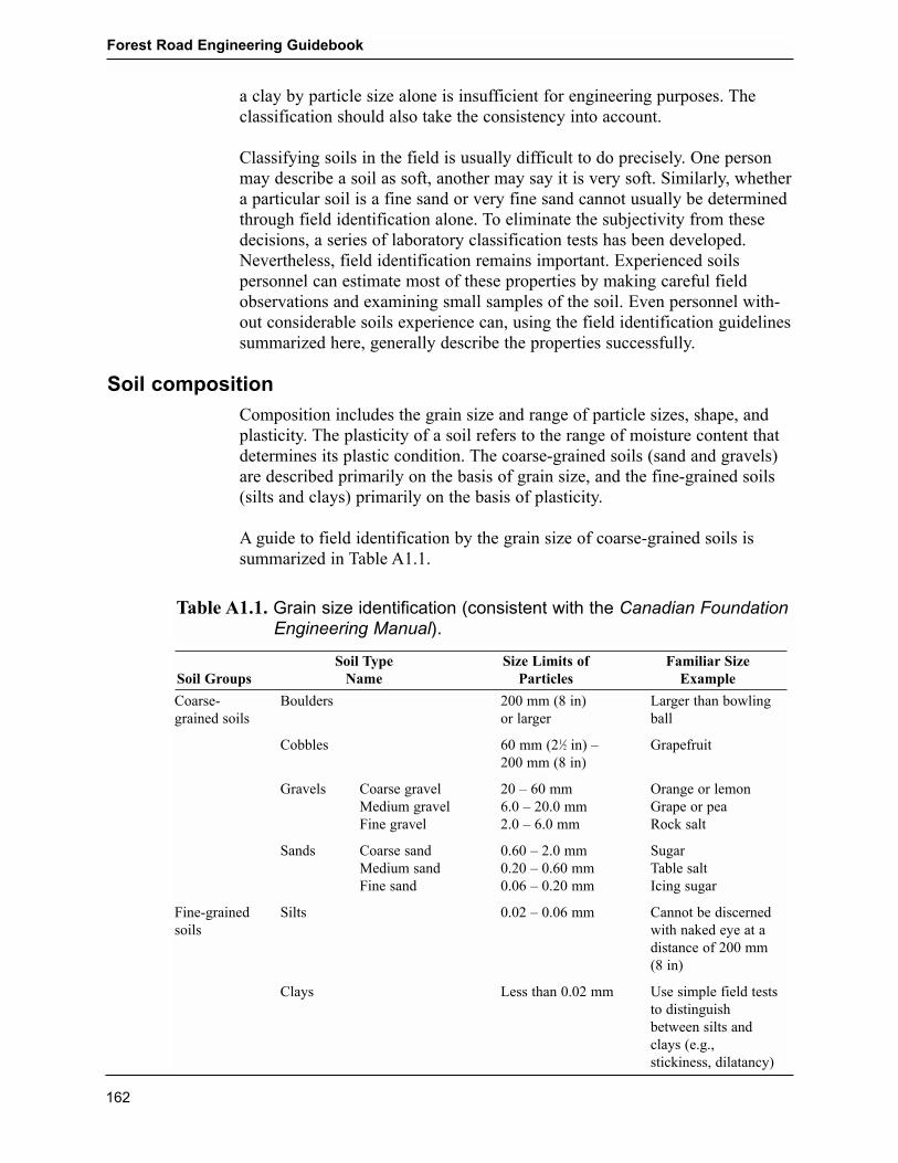
Composition includes the grain size and range of particle sizes, shape, andplasticity. The plasticity of a soil refers to the range of moisture content thatdetermines its plastic condition. The coarse-grained soils (sand and gravels)are described primarily on the basis of grain size, and the fine-grained soils(silts and clays) primarily on the basis of plasticity.
A guide to field identification by the grain size of coarse-grained soils issummarized in Table A1.1.
Forest Road Engineering Guidebook
162
Soil Type Size Limits of Familiar SizeSoil Groups Name Particles Example
Coarse- Boulders 200 mm (8 in) Larger than bowlinggrained soils or larger ball
Cobbles 60 mm (21Ú2 in) � Grapefruit200 mm (8 in)
Gravels Coarse gravel 20 � 60 mm Orange or lemonMedium gravel 6.0 � 20.0 mm Grape or peaFine gravel 2.0 � 6.0 mm Rock salt
Sands Coarse sand 0.60 � 2.0 mm SugarMedium sand 0.20 � 0.60 mm Table saltFine sand 0.06 � 0.20 mm Icing sugar
Fine-grained Silts 0.02 � 0.06 mm Cannot be discernedsoils with naked eye at a
distance of 200 mm(8 in)
Clays Less than 0.02 mm Use simple field tests to distinguishbetween silts and clays (e.g.,stickiness, dilatancy)
Table A1.1. Grain size identification (consistent with the Canadian FoundationEngineering Manual).

Soil consistency
The consistency of a cohesive soil�described as hard or soft�can be esti-mated from the pressure required to squeeze an undisturbed sample betweenthe fingers. An undisturbed sample is one that is in its natural condition as onor in the ground; it has not been remoulded by any mechanical disturbance,such as bulldozer tracks.
If the soil is brittle (fails suddenly with little movement as it is squeezed), fri-able (crumbles easily), or sensitive (loses much of its strength when remould-ed and then resqueezed), these terms should be included in the description ofthe soil�s consistency.
A guide to estimating consistency in this way is summarized in Table A1.2.
Table A1.2. Consistency field test for cohesive soils.
Field Test Term
Easily penetrated several centimetres by fist. Very softEasily penetrated several centimetres by thumb. SoftPenetrated several centimetres by thumb with moderate effort. FirmReadily indented by thumb but penetrated only with great effort. StiffReadily indented by thumbnail. Very stiffIndented with difficulty by thumbnail. Hard
Soil density
The density of a non-cohesive soil may be estimated in the field by the easewith which a reinforcing rod penetrates the soil. It is quoted in relative terms,such as loose or dense. A guide to estimating soil density is summarized inTable A1.3.
Table A1.3. Soil density field test for non-cohesive soils.
Field Test Term
Easily excavated with spade. Very loose
Easily penetrated with 13 mm (0.5 in) reinforcing rod pushed by hand or, Loosealternatively, shows some resistance to spade or penetration with hard bar.
Easily penetrated with 13 mm (0.5 in) reinforcing rod driven with a Compact 2.25 kg (5 lb) hammer or, alternatively, shows considerable resistance to spade or penetration with hard bar.
Penetrated 0.3 m (1 ft) with 13 mm (0.5 in) reinforcing rod driven with Dense2.25 kg (5 lb) hammer or, alternatively, shows no penetration with hard bar or requires pick for excavation.
Penetrated only a few centimetres with 13 mm (0.5 in) reinforcing rod Very densedriven with 2.25 kg (5 lb) hammer or, alternatively, shows high resistance to pick.
Forest Road Engineering Guidebook
163

Soil compressibility
A soil�s potential for compressibility is not easy to determine by visual exam-ination alone. This is usually done by laboratory tests. However, if it is sus-pected that the soil will settle considerably under load, this should be reported.
There is a general relationship between consistency (as defined for cohesivesoils) or soil density (as defined for non-cohesive soils) and compressibility.For example, the soft and loose soils are likely to compress considerablyunder loads.
Reporting soil description
In forming a description, the predominant particle size is what is used todescribe the soil type. The relative content of other particle sizes modifies thedescription (e.g., sand GRAVEL with some silt).
A predominantly coarse-grained soil is termed either a gravel or a sand,depending on which component appears to be the more abundant. The lessabundant component and the fines are used as modifiers; the least importantcomponent is stated first. For example, a soil with 30% fines (silt), 45%gravel, and 25% sand would be best described as sandy, silt GRAVEL.The terms in Table A1.4 are used to indicate various proportions by weightwithin the respective grain-size fractions.
Table A1.4. Soils description terms.
ExampleDescriptive Term by Weight Proportion
NOUN GRAVEL, SAND, SILT, CLAY >50%�and� and gravel, and silt, etc. >35%
ADJECTIVE gravelly, sandy, silty, clayey, etc. 20�35%
�Some� Some sand, some silt, etc. 10�20%
�Trace� Trace sand, trace silt, etc. 1�10%
For example:
� A �silty CLAY, trace of fine sand� would be >50% clay, 20�35% silt, and0�10% sand.
� A �sandy GRAVEL with some cobbles� would be >50% gravel with20�35% sand sizes and 10�20% cobbles.
Forest Road Engineering Guidebook
164

Appendix 2. Vertical (parabolic) curves
The relative flatness, or �K� value of a vertical (parabolic) curve, is the hori-zontal length over which there is a 1% change of grade. The minimum lengthof a vertical curve is solved as the K value times �A,� the algebraic differ-ence between the entry and exit grades (LVC = K*A). When the length of thevertical curve (LVC) is equal to or exceeds the stopping sight distance(SSD), the K value is given by the expression:
Crest
K = SSD2
200(H10.5 + H2
0.5)2
H1 height of driver�s eye: 1.05 mH2 height of object: one-lane road - 1.30 m (vehicle)
two-lane road - 0.15 m (object)
Sag
K = SSD2
200 (H3 + SSD Tan1°)H3 height of headlight: 0.6 m
Forest Road Engineering Guidebook
165
Crest Crest Sag
Design speed Minimum Minimum (km/h) SSDa (m) One-lane SSD (m) Two-lane One-lane
20 40 1.7 20 1.0 2.130 65 4.5 35 3.1 5.140 95 9.6 50 6.3 8.550 135 19.4 70 12.3 13.460 175 32.7 90 20.3 18.770 220 51.6 110 30.3 24.080 270 77.8 135 45.7 30.8
a Values of minimum stopping sight distance apply to one-lane, two-way roads. For two-lane and one-lane,one-way roads, multiply the values of minimum SSD by a factor of 0.5.
Table A2.1. Minimum K values, where LVC > SSD.

When the LVC is less than the minimum SSD, the K values are solved by theexpression:
Crest
K = 2SSD 200(H1
0.5 + H20.5)2
A A2
Sag
K = 2SSD 200(H3 + SSD Tan 1°)
A A2
Forest Road Engineering Guidebook
166
Crest curve: One-lane, two-way roadA
2 3 4 5 6 7 8 9 10 11 12 13 14 15 16 17 18 19
20 0.2 0.6 0.9 1.2 1.3 1.5 1.6 1.6
30 1.6 2.9 3.6 4.1 4.3
40 0.5 5.6 8.0 9.1 9.5
50 8.9 16.5 19.0
60 12.5 28.9 32.5
70 42.5 51.4
80 35.7 75.9
Table A2.2. Minimum K values, where LVC < SSD.
Des
ign
spee
d (k
m/h
)

Forest Road Engineering Guidebook
167
Crest curve: Two-lane roadA
2 3 4 5 6 7 8 9 10 11 12 13 14 15 16
20 0.3 0.6 0.7 0.8 0.9 0.9
30 0.6 1.9 2.5 2.9 3.0
40 0.1 4.1 5.6 6.1
50 2.4 10.1 12.1
60 15.7 20.1
70 10.3 29.0
80 35.3
Des
ign
spee
d (k
m/h
)
Sag curve: One- and two-lane road
A
2 3 4 5 6 7 8
20 0.4 1.4 1.8 2.0
30 2.4 4.3 4.9
40 0.6 6.6 8.2
50 6.2 12.2
60 11.8 17.9
70 17.3 23.5
80 24.3 30.5
Des
ign
spee
d (k
m/h
)

Table A2.3. Vertical curve elements (crest curve, single-lane road).
Aa 20 km/h 30 km/h 40 km/h 50 km/h 60 km/h 70 km/h 80 km/h
Crest curve: single-lane road
2 71
3 38 128 228
4 36 116 206 311
5 3 83 163 258 388
6 34 114 196 310 467
7 68 136 229 361 544
8 13 73 156 261 413 622
9 26 86 175 294 465 700
10 36 96 194 327 516 778
11 45 106 214 359 568 856
12 2 52 116 233 392 620 933
13 8 58 125 263 425 671 1011
14 13 63 136 272 457 723 1089
15 18 68 144 292 490 775 1167
16 21 72 154 311 523 826 1244
17 25 77 164 331 555 878 1322
18 28 81 173 350 588 929 1400
19 31 86 183 369 621 981 1478
20 33 90 193 389 653 1033 1555
21 36 95 202 408 686 1084 1633
22 37 99 212 428 719 1136 1711
23 39 104 221 447 751 1188 1789
24 41 108 231 467 784 1239 1867
Minimum 40 65 95 135 175 220 270SSD (m)
a Algebraic difference between the entry and exit grades (%).
Forest Road Engineering Guidebook
168

Table A2.4. Vertical curve elements (crest curve, double-lane road).
Aa 20 km/h 30 km/h 40 km/h 50 km/h 60 km/h 70 km/h 80 km/h
Crest curve: double-lane road
2 21 71
3 7 47 87 137
4 40 80 121 183
5 20 60 102 152 229
6 4 34 74 122 182 274
7 13 43 86 142 212 320
8 20 50 98 163 243 366
9 26 56 111 183 273 411
10 30 63 123 203 303 457
11 4 34 69 135 223 334 503
12 7 37 75 147 244 364 548
13 9 40 82 160 264 394 594
14 12 43 88 172 284 425 640
15 13 46 94 184 305 455 686
16 15 49 100 197 325 486 731
17 17 52 107 209 345 516 777
18 18 55 113 221 366 546 823
19 19 58 119 233 386 577 868
20 20 61 125 246 406 607 914
21 21 65 132 258 427 637 960
22 22 68 138 270 447 668 1006
23 23 71 144 283 467 698 1051
24 24 74 150 295 488 728 1097
MinimumSSD (m) 20 35 50 70 90 110 135
a Algebraic difference between the entry and exit grades (%).
Forest Road Engineering Guidebook
169

Table A2.5. Vertical curve elements (sag curve).
Aa 20 km/h 30 km/h 40 km/h 50 km/h 60 km/h 70 km/h 80 km/h
Sag curve
2
3 2 19 35 52 73
4 9 26 49 71 94 122
5 2 22 41 67 93 120 154
6 8 30 51 81 112 144 185
7 13 35 59 94 131 168 216
8 16 40 68 108 149 192 247
9 19 46 76 121 168 216 277
10 21 51 85 134 187 240 308
11 23 56 93 148 205 264 339
12 25 61 102 161 224 288 370
13 27 66 110 175 243 312 401
14 30 71 119 188 261 336 432
15 32 76 127 202 280 360 462
16 34 81 136 215 298 384 493
17 36 86 144 229 317 408 524
18 38 91 153 242 336 432 555
19 40 96 161 256 354 456 586
20 42 101 170 269 373 480 616
21 44 106 178 282 392 504 647
22 46 111 187 296 410 528 678
23 48 116 195 309 429 552 709
24 51 121 204 323 448 576 740
Minimum 20 35 50 70 90 110 135SSD (m)
a Algebraic difference between the entry and exit grades (%).
Forest Road Engineering Guidebook
170

Appendix 3. Plotting data: plan and profile information
Plans/profiles and plotted cross-sections should be completed for the fieldsurvey. The plans and profiles should be prepared in 1 km sections on a 1 mplan/profile sheet with a minimum 200 m overlap between drawings. Theplan/profile should be drawn to a scale of 1:2000 horizontally and 1:200 ver-tically.
The example plan/profile drawing in this appendix illustrates the plan andprofile information requirements listed below. The drawing is available at thefollowing Ministry of Forests website:http://www.for.gov.bc.ca/tasb/legsregs/fpc/fpcguide/guidetoc.htm
Plans should include all information pertinent to the project:� north arrow with magnetic declination shown
� preliminary line traverse (include turning points, TPs)
� accumulated chainage and TP number at every fifth TP
� overlap between plans of 200 m
� chainage equations
� reference points and benchmarks plotted and labelled
� existing roads complete with road name
� existing structures (bridges, culverts, buildings, fences, etc.)
� existing services and utilities including but not restricted to telephone,power, gas, oil, sewer and water lines, and fences
� percent side slope and direction
� terrain features and direction (rock outcrops, creeks, rivers, swamps, wetareas, riparian zones, etc.)
� timber types, number, diameter, and species or stumps within the clearingwidths
� designed L-line complete with curves
� curve information including radius (R), angle of intersection (IC), lengthof curve (LC), beginning of curve (BC), and end of curve (EC)
� accumulated L-line chainage at beginning and end of curves
� bearing of the L-line tangents shown on the plan to the nearest 30 sec-onds
� kilometre stations on the L-line
� 100 m of existing road alignment from junction or extension of existingpoints
� clearing and right-of-way boundaries
Forest Road Engineering Guidebook
171

� title block indicating road name, kilometre, date of survey, and scale(horizontal and vertical)
� special notes indicating land district, road width, survey level, and datumof elevation
� all legal boundaries and plan numbers
� all monumentation found and tied within 300 m of the P-line, including atraverse tie table.
A key map should also be included on the first drawing of the set to a scaleof 1:50 000. Note that no curves are required where I is less than or equal to 5°.
Profiles should include the following information:� chainage and elevation equations
� description of soils (at least every 200 m or at soil change)
� terrain features (creeks, rivers, swamps, wet areas, riparian areas, etc.)
� penetration depths at swamps and wet areas to solid ground, if possible
� grade lines completed with percent grades labelled (adverse or negative)
� grade breaks at grade changes of 2% or less
� vertical curves at grade changes greater than 2%
� turnout locations and dimensions
� design notes (extra ditching, lateral ditching, road widenings, etc.)
� culvert locations with recommended diameter, length, and skew
� kilometre stations
� primary excavation and primary embankment volumes summarized inbank cubic metres at 200 m intervals
� secondary embankment (gravel) volumes summarized in bank cubicmetres at 200 m intervals
� waste and borrow locations, quantities in bank cubic metres, and quantitymovements
� scale: H = 1:2000; V = 1:200
� 100 m of existing road grade and horizontal alignment at junction
� balance points and direction of material movement
� position of cut and fill slope changes
Forest Road Engineering Guidebook
172

� PWL and HWL, where applicable
� span lengths for bridges
� all control points
� design templates
� K values if used for vertical curves.
Forest Road Engineering Guidebook
173

Forest Road Engineering Guidebook
174

Forest Road Engineering Guidebook
175

Forest Road Engineering Guidebook
176

Forest Road Engineering Guidebook
177
Appendix 4. Statement of construction conformance
���� �����!�"������#�����"��!�� �#�$"������#������!�%�� ����&'���"��(��������)�*��
����#�����+������������������������ �������������������
����#�����,����!�#�����-���.�- � ���- �/ 0�#����
�������1�����#��2���������� ��� "������ �- �$������#���+ 3��'�#��-���$������#���+
����#�����1��#�������/
� � � � � ������� ������ ����� �����������������������������������������������������������������������������������������������������������������������������
�����������������������������������������������������������������������������������������������������������������������
�����������������������������������������������������������������������������������������������������������������������
�����������������������������������������������������������������������������������������������������������������������
����������������������������������������������������������������������������������������������������������������������
0�����!������(��1��� ��1�4�� �/� � � � � ���������������������������������������������������������������������������������������������������������������������������������
������������������������������������������������������������������������������������
�������������������������������������������������������������������������������������
�������������������������������������������������������������������������������������
�������������������������������������������������������������������������������������
������������������������������������������������������������������������������������
����������������� �����������������������!�������"���������� �����#���$��������������$����%����&�����������������������' �������������$�(������������� (� �����������#������$������� ����� ��������������(���)�� ��������&�$���������"��������' �����%&������$�(��(��������((����(����������������������$��������������$����%����&��$�(�������������!��������(��(��������*!��+��������������� �%�"�����������������������������)����������������� (�������������(������' �����%&�!��"�!������������� ���������,"�)�(�����-,�
����&�$������������$�������� �����.% ������� (� ����������������(�������(�������������������������"��$�(���(�����������
$$��(%���� $$���������( �����"���(� ������������������������"����(��� $$����������((�$��(��������$���(��%&�����$$��$����� ������&/
�� � ���(�����������������������%����(������� ����$$��$������������ ���������(����� (��������#/����� �������(���������������������������"��$�(���(���������� $$���������( ������$��$������������
$���(�"���(� ������������������������"�����%������( ������������#��������������������(����� (���������������#���0�.% ���1������������(����&����(��%������� $$��������( ������
2�� ����������"�0�������������1������������������������������#�������$���(�������3�������������%��(������(����*�+"�������$$��(%��4�(������������(����&�%&"�������������(���������"���������������$�����������������������$��������������������*��$$��$����+����(����������������.% ������� (� ���������������(�������(�����������$$�������������(����� (������������"��$�(���(���������������� $$��������( ������$��$�������������$���(��
)���� ������������������ ��������������������!�������
������������������� ��������������������!�������
��������������� � � � �
�25 ��)�6� �
7777��������������
� � � � ��������������
������|�������| �� ����� ���������!����
��8�7 �9)��2� �2���2��� ))�*�������������
� � � � �
�:�� ����
� � � � �!2;����� � � � �
.�2�8�2��� ))� � � � �
�����%���<==-

Forest Road Engineering Guidebook
178

Appendix 5. Tables to establish clearing width
Clearing width
The clearing width is shown in Figure 2 of Chapter 1, �Road Layout andDesign.� Since clearing width calculations are straightforward, but verytedious, Tables A5.1 to A5.7 and accompanying Tables A and B have beendeveloped for your convenience.
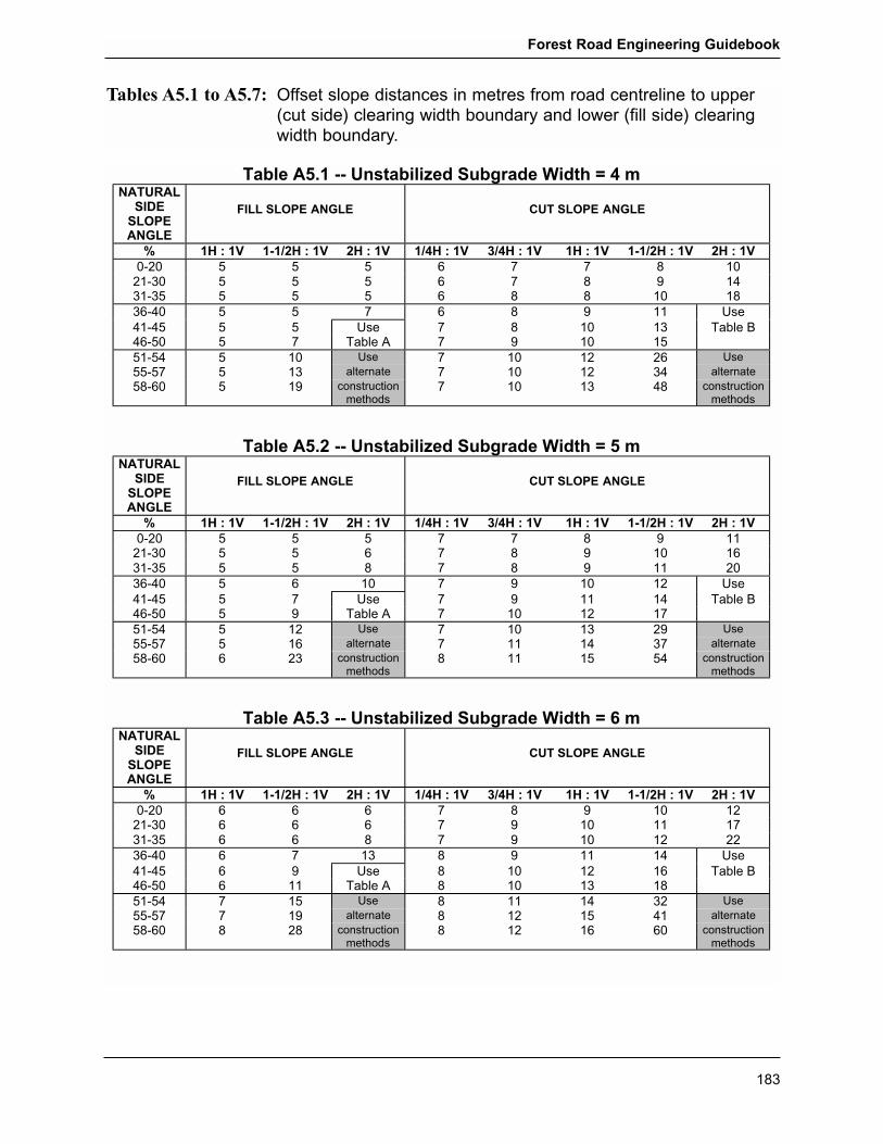
These tables provide slope distances (not the horizontal distances) for estab-lishing suitable offset distances from road centreline to facilitate easy fieldmarking of the upper and lower clearing width boundaries. Note that the off-set slope distances in the tables depend on several factors:
� unstabilized subgrade width
� side slope angle of the natural ground surface
� angles of the fill and cut slopes.
Using the tables in this appendix, the clearing width is the sum of the widthdetermined from the tables and any additional width to account for specialcircumstances (see �Additions to clearing width� in this appendix). Theclearing width established from these tables may be expressed as:
Clearing width = offset distance on cut side of centreline (from tables) +offset distance on fill side of centreline (from tables) +additional width (if necessary)
For a specific subgrade width, these tables assume:
� no horizontal or vertical adjustments at the road centreline
� 0.3 m overburden thickness
� 3 m clearing allowance above the top of the cut slope to standing timber
� selection of the appropriate cut and fill slope angles
� a ditch depth of 0.5 m
� sidecast road construction with little or no longitudinal movement ofmaterial
� a minimum 3 m distance from the road shoulder to the lower side clear-ing width boundary.
� where there is road fill, the toe of the fill slope demarcates the lowerclearing width boundary. Therefore, to establish the clearing width whenusing these tables, include additional width allowances as required (e.g.,additional width will be required for debris and slash disposal on thelower side of the road below the toe of the fill slope).
Forest Road Engineering Guidebook
179
Where the offset slope distance from the road centreline to the upper orlower clearing width boundaries exceeds 50 m, consider using alternative construction methods, such as retaining walls, to reduce the clearing widthrequirements.
Determining clearing width from tables in this appendix
The following procedure is recommended:
1. Select the appropriate unstabilized subgrade width table (the tables havebeen developed for unstabilized subgrade widths of 4, 5, 6, 7, 8, 9, and10 m). This is done:
� after adjusting the road subgrade width to compensate for cuts or fills(see �Adjustments to road subgrade width to compensate for cuts andfills at road centreline�)
� after adjusting the road subgrade width to compensate for road sur-facing materials (see �Additions to clearing width� in this appendix).
2. Choose the appropriate natural side slope angle in the selected subgradewidth table.
3. Based on the expected soil type to be encountered during road construc-tion, choose the appropriate cut and fill slope angles for application in thetables. Details about selecting cut and fill slope angles for road design aregiven in Appendix 1, �Field identification of soils.�
4. To establish the upper clearing width boundary, read the offset slope dis-tance from the appropriate cut slope angle column�the offset distancegiven in the cut slope angle column is a slope distance between the roadcentreline and the upper clearing width boundary.
5. Use a two-step procedure to establish the lower clearing width boundary.Firstly, read the offset slope distance from the appropriate fill slope anglecolumn�the offset distance given in the fill slope angle column is aslope distance between the road centreline and the toe of any fill slope.Secondly, include any additional width allowances such as those for slashdisposal on the lower side of the road below the toe of the fill, sight dis-tance, etc., as explained in �Additions to clearing width� in this appendix.
Adjustments to road subgrade width to compensate for cuts and fillsat road centreline
Use of an adjusted road subgrade width in these tables for short sections ofanticipated cuts or fills at the road centreline should be limited to the obviouslocations in the field, such as where cuts are required through small ridges orfills across linear slope depressions less than 3 m deep. For longer sections ofroad through areas with deep gullies or high ridges, a geometric road designshould be completed and the clearing width determined from these drawings.
Forest Road Engineering Guidebook
180

1. To compensate for a cut at the centreline, adjust the road subgrade widthas follows: Add 1 m to the subgrade width for every 0.3 m cut incrementat centreline to determine the offset slope distance on the cut side of cen-treline. Subtract 1 m from the subgrade width for every 0.3 m cut incre-ment at centreline to determine the offset slope distance on the fill side ofcentreline.
For example, consider a 0.6 m deep cut at centreline on a 6 m wideunstabilized subgrade (assume no surfacing material is applied to the sub-grade). Assume a natural side slope angle of 35% above and below theroad centreline, and fill and cut slope angles of 11Ú2H : 1V and 1H : 1V,respectively. In this case, adjust the unstabilized subgrade width by 2 mas follows:
� Choose the appropriate cut slope angle column from Table A5.5 (8 mwide unstabilized subgrade) to determine the offset slope distance onthe cut side of centreline. The offset slope distance from this table is12 m.
� Choose the appropriate fill slope angle column from Table A5.1 (4 mwide unstabilized subgrade) to determine the offset slope distance onthe fill side of centreline. The offset slope distance from this table is 5 m.
In this cut example, the clearing width (magnitude) is unchanged, but isshifted upslope with respect to the road centreline.
If, because of shallow side slopes, the 0.6 m cut resulted in a through-cutinstead of a fill slope, use the appropriate cut slope angle column fromTable A5.1 (4 m wide unstabilized subgrade) to obtain the required offsetslope distance from centreline to the lower clearing width boundary.
2. To adjust for fills at the centreline, reverse the above procedure. Forexample, to allow for a 0.6 m fill at centreline on a 6 m wide road, adjustthe unstabilized subgrade width by 2 m as follows:
� Choose the appropriate cut slope angle column from Table A5.1 (4 mwide unstabilized subgrade) to determine the offset slope distance onthe cut side of centreline.
� Choose the appropriate fill slope angle column from Table A5.5 (8 mwide unstabilized subgrade) to determine the offset slope distance onthe fill side of centreline.
Additions to clearing width
Compensate for surfacing or ballasting material:Before selecting the appropriate unstabilized subgrade width table, compen-sate for the thickness of surfacing or ballasting material anticipated to beplaced over the unstabilzed subgrade surface. For example, where surfacingmaterial is needed to provide a finished road-running surface, select a wider
Forest Road Engineering Guidebook
181

unstabilized subgrade width when determining the clearing width from thetables in this appendix. For every 0.3 m of surfacing depth, allow for anadditional 1.0 m of unstabilized subgrade width.
For example, to obtain a 4 m wide finished road-running surface on subgradesoils that will require a 0.3 m thickness of gravel, select Table A5.2 (5 mwide unstabilized subgrade).
Compensate for other requirements:Calculate the extra width required for turnouts, sight distance, snow removal,slash disposal, etc. required on the fill side of road centreline. To determinethe lower clearing width boundary, add this extra width to the offset slopedistance (fill side of centreline) given in the tables.
For example, if winter use of the road will require snow ploughing, thestanding timber should be at least 4 m or more away from the road shoulder.Since the tables will only provide for a minimum of 3 m from the roadshoulder to the lower clearing width boundary, simply add the additional 1 or2 m to the offset slope distance. Where natural side slope angles are greaterthan 20% the extra width allowance should be converted to a slope distance,rounded up to the nearest metre, and then added to the offset slope distancedetermined from the tables.
Forest Road Engineering Guidebook
182
Forest Road Engineering Guidebook
183
Tables A5.1 to A5.7: Offset slope distances in metres from road centreline to upper(cut side) clearing width boundary and lower (fill side) clearingwidth boundary.
5���������66�7�������8����� ���9��*�:��� -�57��0�,1��0)3��-�0�
�,00��0)3���-�0� "75��0)3���-�0�
; �<�/��= �6�.�<�/��= �<�/��= �.�<�/��= �.�<�/��= �<�/��= �6�.�<�/��= �<�/��=
=.<= > > > ? @ @ A -=<-.,= > > > ? @ A B -C,-.,> > > > ? A A -= -A
,?.C= > > @ ? A B -- D��
C-.C> > > D�� @ A -= -, 5%����C?.>= > @ 5%���2 @ B -= ->
>-.>C > -= D�� @ -= -< <? D��
>>.>@ > -, ������� @ -= -< ,C �������
>A.?= > -B (����� (�����������
@ -= -, CA (����� (�����������
5���������66�7�������8����� ���9��*�:��� -�57��0�,1��0)3��-�0�
�,00��0)3���-�0� "75��0)3���-�0�
; �<�/��= �6�.�<�/��= �<�/��= �.�<�/��= �.�<�/��= �<�/��= �6�.�<�/��= �<�/��=
=.<= > > > @ @ A B --<-.,= > > ? @ A B -= -?,-.,> > > A @ A B -- <=
,?.C= > ? -= @ B -= -< D��
C-.C> > @ D�� @ B -- -C 5%����C?.>= > B 5%���2 @ -= -< -@
>-.>C > -< D�� @ -= -, <B D��
>>.>@ > -? ������� @ -- -C ,@ �������
>A.?= ? <, (����� (�����������
A -- -> >C (����� (�����������
5���������66�7�������8����� ���9��*�:�>� -�57��0�,1��0)3��-�0�
�,00��0)3���-�0� "75��0)3���-�0�
; �<�/��= �6�.�<�/��= �<�/��= �.�<�/��= �.�<�/��= �<�/��= �6�.�<�/��= �<�/��=
=.<= ? ? ? @ A B -= -<<-.,= ? ? ? @ B -= -- -@,-.,> ? ? A @ B -= -< <<
,?.C= ? @ -, A B -- -C D��
C-.C> ? B D�� A -= -< -? 5%����C?.>= ? -- 5%���2 A -= -, -A
>-.>C @ -> D�� A -- -C ,< D��
>>.>@ @ -B ������� A -< -> C- �������
>A.?= A <A (����� (�����������
A -< -? ?= (����� (�����������

Forest Road Engineering Guidebook
184
5���������66�7�������8����� ���9��*�:�?� -�57��0�,1��0)3��-�0�
�,00��0)3���-�0� "75��0)3���-�0�
; �<�/��= �6�.�<�/��= �<�/��= �.�<�/��= �.�<�/��= �<�/��= �6�.�<�/��= �<�/��=
=.<= @ @ @ A B B -= -,<-.,= @ @ A A B -= -< -B
,-.,> @ @ -= A -= -- -,
,?.C= @ A D�� A -= -< -C D��C-.C> @ -- 5%���2 A -- -< -? 5%����C?.>= @ -C A -- -C <=
>-.>C A -A D�� B -< -> ,> D��
>>.>@ A <, ������� B -, -? CC �������
>A.?= B ,, (����� (�����������
B -, -@ (����� (�����������
5���������66�7�������8����� ���9��*�:�@� -�57��0�,1��0)3��-�0�
�,00��0)3���-�0� "75��0)3���-�0�
; �<�/��= �6�.�<�/��= �<�/��= �.�<�/��= �.�<�/��= �<�/��= �6�.�<�/��= �<�/��=
=.<= @ @ @ A B -= -- -C<-.,= @ @ B A -= -- -< <=
,-.,> @ A -- A -= -< -C
,?.C= @ -= D�� A -- -, -? D��C-.C> A -< 5%���2 B -- -C -A 5%����C?.>= A -? B -< -> <<
>-.>C B <- D�� -= -, -@ ,A D��
>>.>@ -= <@ ������� -= -C -A CB �������
>A.?= -- ,B (����� (�����������
-= -C -B (����� (�����������
5�������>�66�7�������8����� ���9��*�:�A� -�57��0�,1��0)3��-�0�
�,00��0)3���-�0� "75��0)3���-�0�
; �<�/��= �6�.�<�/��= �<�/��= �.�<�/��= �.�<�/��= �<�/��= �6�.�<�/��= �<�/��=
=.<= A A A B -= -- -- -C<-.,= A A -= B -- -< -, <-
,-.,> A -= -, B -- -, ->
,?.C= A -< D�� B -< -C -@ D��C-.C> B -> 5%���2 -= -< -> <= 5%����C?.>= -= -B -= -, -? <,
>-.>C -= <C D�� -= -C -A C- D��
>>.>@ -- ,- ������� -= -> -B >, �������
>A.?= -< C> (����� (�����������
-- -? <= (����� (�����������

Forest Road Engineering Guidebook
185
5�������?�66�7�������8����� ���9��*�:���� -�57��0�,1��0)3��-�0�
�,00��0)3���-�0� "75��0)3���-�0�
; �<�/��= �6�.�<�/��= �<�/��= �.�<�/��= �.�<�/��= �<�/��= �6�.�<�/��= �<�/��=
=.<= A A A B -= -- -< ->
<-.,= A B -- B -- -< -C,-.,> A -- -> -= -< -, -? D��
,?.C= B -, D�� -= -< -C -A 5%����C-.C> -= -? 5%���2 -= -, -? <-C?.>= -- <- -= -C -@ <>
>-.>C -< <@ D�� -- -> -B C> D��
>>.>@ -, ,? ������� -- -? <- >A �������
>A.?= -C >= (����� (�����������
-- -@ << (����� (�����������
������������� ������������������ ����� ������������������ ����������������
5����� ����������$�������(�������</�=�!���������������
-�57��0�,1��0)3��-�0�
D���%���E���) %�����F����
G C�� >�� ?�� @�� A�� B�� -=��
,?.,A -, -> -@ -B
C= D����%����%��� -? -A <- <,
C< B -, -? -B << <> <ACC -< -@ << <? ,= ,C ,@
C? <= <A ,> C- C? >=
CA CC D�����������(����� (������������
5����% ����������$�������(�������</�=�#��������������
-�57��0�,1��0)3��-�0�
D���%���E���) %�����F����
G C�� >�� ?�� @�� A�� B�� -=��
<-.<> -@<?.<A <=,= D����%����%��� <<
,< <= <- <, <C,C << <C <> <@
,? -B <- <, <> <@ <B ,-,A << <C <@ <B ,< ,C ,?
C= <? <B ,< ,> ,A C-C< ,< ,? ,B C, C@ >=
CC C< >< D�����������(����� (������������

Forest Road Engineering Guidebook
186

Forest Road Engineering Guidebook
187
Appendix 6. Sample road inspection and maintenancereport
���������������������������������������
��������������������������� ����� � �� ������� �� ����� ������ �
� �������� � � ����������� �� ����� ������� �� ����� ���� �
��������� �������� � ������������ �
���
�� ��������� ������ � ������������ �� ���� � �� � �� ������� ��� �
!���� " ����������������� #�$��%��� ���&�'������(���� �������
�
�
�
�$��%����# ���'��# �� )��������� ����(����������� #��'��� ������������������ �!�"� ���!�� ���"���#��
• ��������� � ��!������ "#�$� • % ��� ���� �� ��� �������� ��� ���� &"�$�
• '������� ������ "#�$( • '��!�������� �� ����� ��� &"�$(
• )��������� ������ "#�$( • '��!������ ������� &"�$*
• "��������� ���� ����!������ "#�$+ • '��!���� ���,�������� � ��� &"�$+
• "������������ "#�$� • '��!����� � ��� &"�$�
• )�������� "#�$- • ���.� ��������!������!���� &"�$-
• "���� ����� ������������������ �� "#�$� • &�������� ������ ��� ����� ��� &"�$�
• / ����� "#�$0 • ���.� ���������� ������!���� &"�$0
� �$����%���� • 1������2���������� ��������� �����!���� &"�$3
• &���������� ���� ���� �� ��.� �� 4"�$� • &������������� &"��$
• 5����� 4"�$( • &��������������������������6��� ��6�!���� ���� &"���
• / ��� �� 4"�$* • &����������������� &"��(
• 4�����������!������������� 4"�$+ ��%��&!�'������ ��
• /������������� 4"�$� • )�������� �����!����������� ��������� )5�$�
• & � �������� ���� 4"�$- • #� ��.� ������������ )5�$(
• 4 ������ �������� 4"�$� � �$���%��"�
• "���������� ���������� ������ 4"�$0 • "�������� ���� "��$�
• &��� 4"�$3 • 7������� "��$(
��!$ �����%��� • "� ��� ���� ���������� "��$*
• � / ���� ������������������� ��������� 7"�$� • ������� ��� 2 ����������� �6������6������ "��$+
• � 7� ��������� ������������� !��� ������� 7"�$( • �� ���������������� "��$+
• � /������������������������ ������ ���� 7"�$* • 4 ��� ������.������������ "��$-
• � 4�������� � ������������� � ���8�� ������������ 7"�$+
• � & � ����������� ����������� 7"�$�
• � 9� !����������������������� 7"�$-

Forest Road Engineering Guidebook
188
( ���! ��)*#+
��,��
� - �$�������������������
��#�$!���. �*��� ���
� #/����$��"������
��#�$!���. �*�
� #/����$������
� � �
� � � �
� � � �
� � � �
� � � �
� � � �
� � � �
� � � �
� � � �
� � � �
� � � �
� � � �
� � � �
� � � �
� � � �
� � � �
� � � �
� � � �
� � � �
� � � �
� � � �
� � � �
� � � �
� � � �
� � � �
� � � �
� � � �
� � � �
� � � �
� � � �
� � � �
� � � �
� � � �
� � � �
� � � �
� � � �
� � � �
� � � �
� � � �
� � � �
� � � �
� � � �
� � � �
� � � �
� � � �
� � � �
� � � �

Forest Road Engineering Guidebook
189
����� ����� ����������������$��%��� ��
�
�
�
�
�
�
�
�
�
�
�
�
�� ��������������������������� ���
�
�
�
�
�
�
�
�
�
�
�
�
�
�
�
�
�
�
�
�
����" ##� #�$��%��� ��
$��%��� � � � � �������� �����������%������ : ; &
����" ##� #�� �%��� �� #
������������������
* � ��
$��%��� � � � � �������� ����������%������ : ; &

Forest Road Engineering Guidebook
190

Forest Road Engineering Guidebook
191
Appendix 7. Sample road deactivation inspection report
ROAD DEACTIVATION INSPECTION REPORT�������������������������� ����� � �� ������� �� ����� ������ �
� �������� � � ����������� �� ����� ������� �� ����� ���� �
��������� �������� � ������������ ����� �� ��������� ������ � ������������ �� ���� � �� � �� ������� �
� �
!���� " ����������������� #�$��%��� ��
�����+�� ��������%� ��$�# ���� �
�����������������
���������� ������������� ��������
�������������������
���� ���� ����
������������������ !�������"
���������������#�������"�"�������"<
�
�$��%����# ���'��# �� )��������� ����(����������� #��'��� ���=�*�#���7� � ���3��� ���9����&� � ���
• 4 �������� �� ����������������!���������� &=�$� • � 4��!���� ����� ���� ���� &/�$�
�������B • � 4 ������ �������� &/�$(
• � 5���� � �� ������ &"�$� • � "���������� ���������� ������ &/�$*
• � '������� ������ &"�$( • � '������������������� � &/�$+
• � )��������� ������ &"�$* • � &�������� ��������� � &/�$�
• � "�������� ���� ����!������ &"�$+ • � >?�����!������������������� ���� &/�$-
����!��B • � &��������������������������6��� ��6�!���� ���� &/�$�
• � &� ���! ����� ���������������� �� &4�$� • � 7������� ������� �����!������������ � &/�$0
• � "� ��� ���� ����������������� &4�$( • � "��� ��������������������� �������� �������
�� ������������������������� �����@������6
�33��
&/�$3
• � ������� ��� 2 ������������������ �6
�����6������
&4�$*
( ���! ��)*#+
��,��
� - �$
"� ������.���"�� ��#�$!���. �*��� ���
� #/����$��"������
��#�$!���. �*�
� #/����$������
� � � �
� � � �
� � � �
� � � �
� � � �
� � � �

Forest Road Engineering Guidebook
192
( ���! ��)*#+
��,��
� - �$
"� ������.���"�� ��#�$!���. �*��� ���
� #/����$��"������
��#�$!���. �*�
� #/����$������
� � � �
� � � �
� � � �
� � � �
� � � �
� � � �
� � � �
� � � �
� � � �
� � � �
� � � �
�
����� ����$��%��� ��� �������
�
�
�
�
�
�
�
�
�
�� ��������������������������� ���
�
�
�
�
�
�
�
�
�
�
����" ##� #�$��%��� ��
$��%��� � � � � �������� �����������%������ � � �
����" ##� #�� �%��� �� #
��������* � ��
$��%��� � � � � �������� ����������%������ � � �

Forest Road Engineering Guidebook
193
App
endi
x 8.
Exa
mpl
e fie
ld d
ata
form
for
dea
ctiv
atio
n fie
ld a
sses
smen
ts
4 ��� �
��,�4 �������<�����������������������������������������������������������������
5 ��<�AAAAA���AAAAA
& ��<����������������������������������������������������������������������������������������������������
4���������<��������������������������������������������������������������������������������������
/� �������������<���������������������������������������������������������������������������
���
�������
��������
�������
(����� (����
�����( ��&
*�$�����+
����(��$����
�&�%������
��(�������
��(���' �
��������
5�����
�������
�� ���∠
$���$�
*G�+
�� ���∠
�������$�
*G+
���
�������
*G+
���
�����
*�+
!���
���$�
������
*�+
!���
���$�
����
*G+
� �
���$�
������
*�+
� �
���$�
����
*G+
)�%����&�
� ��(�
�������
$��%����H
(�
��$
�
��
����
���
"�&
!��$
���
��!/
�! �
4 ���� ���<��� ��,���
4 ���� ���������6��B(�$�
>����
�������������������������
��,������� �����.�����������
���� ��� � ������������<��#�������� ��6���!����� ��!��� � �������������������� ������������ C���� �����������6� ���������� ���
�.��������������� ��������������������� �����������������
�����
�������������������
������������������6�� ��6� !�� ��6�����������
5��������������������� ���! ���
�������.��
>? �
���<�D�������������6�4;'�����!����� �����!����6�53������3��
���"������ ���������������� ������������ ������)���? �
��6� ��
����������!������ ���������� ���! ���������������
�����E4
��!����� �����!���F� ���E����������F
'������
#��� �������! ����6��������
���������6�����? �
��<� �� ������� ��8������,������������������ � �8�� 2 ��,����.�����,��� ��
� �
�������������������������8���.�����
�������������� ����������!����8� ��
��������.�����
����8��������� ����8������������
!������� ��������������8��� ����������� �������
��������������8��� ���������.��������������� ���� �
�������� ����������� � 8��� ��
� ������������8�������������� �������?����!����8������������������8��!����������������� �8��!������������� ��������,�����8
� ��������8�!���� ��!���!��8��������������� ���� �������� ���� ��8��!������������������������ ������8��!������������� ������
���������������
���� ��� ���������� ������8��� ������� ������ !������8�� ������6�����
���� ��,����
"������ ��� ���� ���������� ��� ������ ��������!���6������ 6�����6������� �����?�������� ��� ��������� ��6�����6�� ��� ����� !��6������
% ��� ��∠�1�����G
��"��� �������� ��� ������ ��� �!��� �����
% ��� ��∠�&�������G
�"��� �������� ��� ������ �������������� ������
4 ���� �������G
��!�� ����� ��������� �
4 �����������
/�������� �
)������������������
H����������������������������������� �
)�������� ������G�
"��� ���������������
'����������������
�I���������������
'������� ������G�
"��� ��������������
"� ������,���� ��������
>? �
���<��'����������� � �6�">������ ���������6�))�������� ������6�H"��� ��������

Forest Road Engineering Guidebook
194

Appendix 9. Example road deactivation prescription content requirements
Examples are presented below showing the linkage between various site andproject conditions and the minimum content of a road deactivation prescrip-tion.
Example 1: A road is prescribed for semi-permanent deactivation with 4-wheel drive vehicle access. The road traverses gentle terrain with no land-slide hazard. There are a few crossings of S6 streams, and some cross-drainculverts on the road. The risk of damage to adjacent resources is low or mini-mal. Deactivation measures are limited to water management techniques(such as cross-ditches, waterbars, and back-up of some stream culverts) andrevegetation of exposed soils using a suitable grass seed and legume mixture.
� Example Prescription Content Requirements: For this project, a scaletopographic map showing the locations of recommended actions corre-sponding to the chainages of field markings may be sufficient for com-munication of the required works to field crews (and review and approvalby the district manager, if required).
Example 2: A road is prescribed for semi-permanent deactivation with 4-wheel drive vehicle access. The road traverses gentle to moderate terrainwith no landslide hazard. There are many culvert and bridge crossings of S5 and S4 streams, and many cross-drain culverts along the road. The soilsare fine-grained and prone to erosion. The area is in a wet belt. The risk ofsediment transport to aquatic resources and aquatic habitat from existing sed-iment sources is high. Deactivation measures include water managementtechniques such as cross-ditches, waterbars, removal or back-up of cross-drainculverts, and removal or back-up of stream culverts, and other measures suchas repair of bridges and revegetation of exposed soils using a suitable grassseed and legume mixture.
� Example Prescription Content Requirements: In this case, the basic mini-mum requirement of a deactivation prescription would be a 1:5000 scalemap (or other suitable scale) showing the locations of the actions corre-sponding to the chainages of field markings, and a tabular summary(spreadsheet) to accompany and complement the map. The tabular sum-mary should provide more detailed information such as general site con-ditions, the size of existing culverts and bridges, sediment transport hazards and consequences, and methods to control sediment transport,including the measured chainages along the road and the correspondingactions. In this case, the prescription should clearly identify the fishstreams and the timing windows for working in and about a stream, asdeveloped and provided by a designated environment official.
Forest Road Engineering Guidebook
195

Example 3: A road is prescribed for semi-permanent deactivation with 4-wheel drive vehicle access. The road is located on a mid-slope, and travers-es steep terrain and areas of moderate to high likelihood of landslides. (Note: A qualified registered professional must prepare a deactivation pre-scription where the road crosses areas with a moderate or high likelihood oflandslides, as determined by a terrain stability field assessment [TSFA].)There are visual indicators of road fill instability, surface soil erosion, andprevious road fill washouts along the road. The road is located in a wet belt,and receives high annual precipitation. The road crosses many deeply incisedS5 streams contained in gullies tributary to an S2 stream downslope of theroad. Deactivation measures include water management techniques such ascross-ditches, and removal or back-up of stream culverts, long segments ofpartial road fill pullback to maintain motor vehicle access, and revegetationof exposed soils using a suitable grass seed and legume mixture. There is anexisting high risk of potential damage to public utilities, a highway, and theS2 stream from potential fill slope failures.
� Example Prescription Content Requirements: This is a more complexproject, involving deactivation prescriptions for unstable terrain.Reporting may include more detailed observations and assessment of ter-rain stability. In this case, the basic minimum requirement of a deactiva-tion prescription would include a 1:5000 scale map showing the locationsof the actions corresponding to the chainages of field markings, a tabularsummary (spreadsheet) to accompany and complement the map, and adetailed letter or report. The prescription should clearly identify the tim-ing windows for working in and about streams that are tributary to the S2stream, developed and provided by a designated environment official.The prescription should also specify the need for any professional fieldreviews during the deactivation work.
Forest Road Engineering Guidebook
196

Appendix 10. Landslide risk analysis
Introduction
This appendix provides:
� an example of a procedure for carrying out a qualitative landslide riskanalysis, including an example qualitative landslide risk matrix (Table A10.1).
� an example of a qualitative landslide hazard table (Table A10.2)
� examples of qualitative landslide consequence tables (Tables A10.3�A10.11)
Landslide risk analysis is a systematic use of information to determine thelandslide hazard (likelihood of landslide occurrence) and the consequence ofa landslide at a particular site, thereby allowing an estimate of the risk toadjacent resources from a landslide occurrence.
Notes:The examples of the qualitative landslide hazard table, landslide consequencetables, and landslide risk matrix provided are for illustration only and shouldnot be considered a procedural standard. The tables and matrix should bemodified, or a different risk-ranking method that varies in detail and com-plexity, should be adapted to suit site-specific requirements.
Qualitative landslide risk analysis satisfies most forestry practice needswhere relative risk rankings are sufficient to provide guidance for decisionmaking. This method of risk analysis, however, has limitations and in somecircumstances it may be advantageous to use a quantitative landslide riskanalysis method.
Landslide risk
Landslide risk = Landslide hazard × Landslide consequence= Likelihood of landslide occurrence × [(Element at risk) ×
(Vulnerability of that element at risk from a landslide)]
Table A10.1 is an example of a qualitative landslide risk matrix for a specificelement at risk. It combines a relative landslide hazard rating and a relativelandslide consequence rating that represents the vulnerability of that elementat risk. The term �vulnerability� refers to the fact that an element at risk maybe exposed to different degrees of damage or loss from a landslide.
Table A10.1 uses a 5 × 3 matrix, consisting of five qualitative ratings of land-slide hazards (VH, H, M, L, and VL) described in Table A10.2, and threequalitative ratings of landslide consequences (H, M, L) described in TablesA10.3�A10.11.
Forest Road Engineering Guidebook
197

Landslide hazard
Landslide hazard is the likelihood of a particular landslide occurring. It isdependent on the type and magnitude of the landslide of significance for aspecified element at risk. The landslide of significance is the smallest land-slide that could adversely affect the element at risk.
For example, if the element at risk is a fish stream, the landslide of signifi-cance is the smallest landslide that could reach, and adversely affect, thestream. The landslide of significance usually has the greatest probability ofoccurrence of any landslide to affect the element at risk. For a specific site,landslides that are smaller or larger than the landslide of significance couldoccur. For example, a smaller landslide event would have a greater likelihoodof occurrence compared to the landslide of significance, but would usuallyhave no adverse effect on a fish stream. Similarly, a larger landslide eventwould have a much smaller chance of occurring compared to the landslide ofsignificance, but would result in greater damage and therefore have anadverse effect on a fish stream.
Different elements at risk often have different landslides of significance. It ispossible that the same element at risk could be potentially subject to two ormore different types of landslides at the same time, and therefore could besubject to two or more different landslide hazards. Assuming the same typeof landslide, the landslides of significance for different elements at risk couldbe quite different, and therefore the hazards could be quite different.
Description of a landslide hazard for forestry purposes should include anestimate of landslide characteristics, such as:
� the likely path of a landslide event
� the dimensions of the transportation and deposition areas
Forest Road Engineering Guidebook
198
Table A10.1. Example of a qualitative risk matrix.
Landslide Risk of Damage to ConsequenceElement at Risk Low Mod High
Very VL VL LLow
Low VL L M
Landslide Mod L M HHazard
High M H VHVery H VH VHHigh

� the type of materials involved (e.g., source area material type)
� the volumes of material removed and deposited.
In Table A10.2, the example of range of annual probability (Column 2)and example of qualitative description for a range of annual probability(Column 3) are only included to give users some physical idea of the mean-ing of the relative qualitative ratings in Column 1.
Additionally, some users may relate better to a 20-year period of time(approximating the life of a logging road) than to an annual probability. Forthis reason, Column 4 in Table A10.2 provides an example of range ofprobability of landslide occurrence for the landslide of significance for aspecific element at risk assuming a 20-year design life. For illustrative pur-poses, the following example shows that a Moderate hazard rating (annualprobability [Pa] of 1/100) corresponds to an 18% chance that at least onelandslide event will occur in 20 years.
Example:
According to probability theory, the long-term probability of occurrence (Px)is related to the annual probability of occurrence (Pa) by the following:
Px = 1-[1-(1/Pa)]x, where Px is the probability of at least one landslideoccurring within the specified time period �x� years.
For a service life of 20 years (i.e., x = 20), and a Pa of 1/100,
P20 = 1-[1-(1/100)]20
= 0.18 or 18%
This means that there is an 18% chance of the 1 in 100-year event occurringwithin the 20-year service life of the road. If the service life of the road isdoubled to 40 years (i.e., x = 40), the chance of the 1 in 100-year eventoccurring within the 40-year service life rises to 33%.
Forest Road Engineering Guidebook
199

Forest Road Engineering Guidebook
200
Table Element at risk
Table A10.3 Human life and bodily harm
Table A10.4 Public and private property (includes building, struc-ture, land, resource, recreational site and resource,cultural heritage feature and value, and other features)
Table A10.5 Transportation system/corridor
Table A10.6 Utility and utility corridor
Table A10.7 Domestic water supply
Table A10.8 Fish habitat
Table A10.9 Wildlife (non-fish) habitat and migration
Table A10.10 Visual resource in scenic area
Table A10.11 Timber value (includes soil productivity)
Landslide consequence
Landslide consequence is the product of the element at risk and the vulnera-bility of that element at risk from a landslide. Tables A10.3�A10.11 areexamples of landslide consequence tables that express consequence in termsof three relative qualitative ratings: H, M, and L. In this scheme, if there isno likely consequence, the consequence is assumed to be less than low, ornil, as appropriate. The elements at risk included in these consequence tablesinclude:

Forest Road Engineering Guidebook
201
Col
umn
(1)
Col
umn
(2)
Col
umn
(4)
Rel
ativ
e qu
alit
ativ
e E
xam
ple
of r
ange
of
Exa
mpl
e of
ran
ge o
fra
ting
of
land
slid
e an
nual
prob
abili
typr
obab
ility
occu
rren
ce(P
a) o
f la
ndsl
ide
of la
ndsl
ide
occu
rren
ce f
orfo
r th
e la
ndsl
ide
of
occu
rren
ce f
or th
eth
e la
ndsl
ide
of s
igni
fica
nce
sign
ific
ance
for
la
ndsl
ide
of s
igni
fica
nce
Col
umn
(3)
for
a sp
ecif
ic e
lem
ent a
ta
spec
ific
ele
men
t fo
r a
spec
ific
ele
men
t E
xam
ple
of q
ualit
ativ
e de
scri
ptio
nri
ska,
c (a
ssum
es a
20-
year
at r
isk
at r
iska,
b,c
for
rang
e of
ann
ualp
roba
bilit
y (P
a)c
desi
gn li
fe)
Ver
y H
igh
(VH
)A
nnua
l pro
babi
lity
Pa o
f 1/
20 in
dica
tes
that
a la
ndsl
ide
is im
min
ent (
or li
kely
to o
ccur
fre
quen
tly)
>64%
cha
nce
that
at l
east
(Pa)
>1/
20fo
r an
exi
stin
g ro
ad, o
r w
ould
occ
ur s
oon
afte
r ro
ad c
onst
ruct
ion
in th
e ca
seon
e ev
ent w
ill o
ccur
of n
ew r
oad
deve
lopm
ent,
and
wel
l with
in th
e lif
etim
e of
the
road
. In
the
case
in 2
0 ye
ars
of p
ast l
ands
lide
activ
ity, l
ands
lides
occ
urri
ng w
ithin
the
past
20
year
s ge
nera
llyha
ve c
lear
and
rel
ativ
ely
fres
h si
gns
of d
istu
rban
ce.
Hig
h (H
)A
nnua
l pro
babi
lity
Pa o
f 1/
100
indi
cate
s th
at a
land
slid
e ca
n ha
ppen
(or
is p
roba
ble)
with
in th
e64
% c
hanc
e th
at a
t lea
st
(Pa)
1/1
00 to
1/2
0ap
prox
imat
e lif
etim
e of
the
exis
ting
or p
ropo
sed
road
. In
the
case
of
past
on
e ev
ent w
ill o
ccur
inla
ndsl
ide
activ
ity, l
ands
lides
occ
urri
ng b
etw
een
20 a
nd 1
00 y
ears
are
usu
ally
20 y
ears
iden
tifia
ble
from
dep
osits
and
veg
etat
ion,
but
may
not
app
ear
fres
h.
Mod
erat
e (M
)A
nnua
l pro
babi
lity
Pa o
f 1/
500
indi
cate
s th
at a
land
slid
e w
ithin
a g
iven
life
time
of th
e ex
istin
g or
18%
cha
nce
that
at l
east
(P
a) 1
/500
to 1
/100
prop
osed
roa
d is
not
like
ly, b
ut p
ossi
ble.
In
the
case
of
past
land
slid
e ac
tivity
,on
e ev
ent w
ill o
ccur
inla
ndsl
ides
occ
urri
ng b
etw
een
100
and
500
year
s m
ay n
ot b
e ea
sily
iden
tifie
d.20
yea
rs
Low
(L
)A
nnua
l pro
babi
lity
Pa o
f 1/
2500
indi
cate
s th
at th
e lik
elih
ood
of a
land
slid
e is
rem
ote
with
in th
e4%
cha
nce
that
at l
east
(Pa)
1/2
500
to 1
/500
lifet
ime
of th
e ro
ad. I
n th
e ca
se o
f pa
st la
ndsl
ide
activ
ity, l
ands
lides
occ
urri
ng
one
even
t will
occ
ur in
betw
een
500
and
2500
yea
rs a
re d
iffi
cult
to id
entif
y.20
yea
rs
Ver
y L
ow (
VL
)A
nnua
l pro
babi
lity
Pa <
1/2
500
indi
cate
s th
at th
e lik
elih
ood
of a
land
slid
e is
ver
y re
mot
e w
ithin
1% c
hanc
e th
at a
t lea
st(P
a) <
1/25
00th
e lif
etim
e of
the
road
.on
e ev
ent w
ill o
ccur
in20
yea
rs
(Mod
ifie
d af
ter
Res
ourc
e In
vent
ory
Com
mitt
ee 1
996)
Not
es:
a. A
ssum
e th
at r
ange
s of
pro
babi
lity
appl
y to
a 1
-km
seg
men
t of
road
.b.
Ann
ual p
roba
bilit
y (P
a) o
f 1/
100,
for
exa
mpl
e, m
eans
an
even
t with
an
estim
ated
ret
urn
peri
od o
f 10
0 ye
ars.
c. T
he e
xam
ple
of r
ange
of
annu
al p
roba
bilit
y(C
olum
n 2)
and
exam
ple
of q
ualit
ativ
e de
scri
ptio
nfo
r a
rang
e of
ann
ual p
roba
bilit
y (C
olum
n 3)
are
onl
yin
clud
ed to
giv
e us
ers
som
e ph
ysic
al id
ea o
f th
e m
eani
ng o
f th
e re
lativ
e qu
alita
tive
ratin
gs in
Col
umn
1.
Tab
le A
10.2
.E
xam
ple
of a
qua
litat
ive
land
slid
e ha
zard
tab
le.
Inte
nded
for
use
in q
ualit
ativ
e la
ndsl
ide
haza
rd a
nd r
isk
anal
yses
for
terr
ain
stab
ility
fie
ld a
sses
smen
ts, a
nd f
or p
repa
ratio
n of
mea
sure
s to
mai
ntai
n sl
ope
stab
ility
and
road
dea
ctiv
atio
n pr
escr
iptio
ns.
Lan
dslid
e ha
zard
is th
e lik
elih
ood
of a
par
ticul
ar la
ndsl
ide
occu
rrin
g. I
t is
depe
nden
t on
the
type
and
mag
nitu
de o
f th
e la
ndsl
ide
of s
igni
fica
nce
for
a sp
ecif
ied
elem
ent a
t ris
k. R
efer
to te
xt f
or f
urth
er d
iscu
ssio
n.

Tables A10.3�A10.11. Examples of qualitative landslide consequence tables.
Intended for use in qualitative landslide hazard and risk analyses for terrainstability field assessments, and for preparation of measures to maintain slopestability and road deactivation prescriptions.
Notes:
� Consequence is the product of the element at risk and the vulnerabilityof that element at risk from a landslide.
� Only a few �examples of factors to consider� are provided. There may beothers depending on the scale of assessment and the project and site con-ditions.
� The tables are examples only and would likely change depending on thescale of assessment (temporary spur road, versus permanent mainline,versus secondary road, versus provincial highway, etc.).
� For most elements at risk, only broad values are applied (e.g., utilizedbuilding or structure versus abandoned building or structure; active trans-portation system/corridor versus non-active transportation system/corri-dor, critical utility, or utility corridor).
� The ratings in the consequence tables for the various elements at riskshould not be compared.
� If there is no likely consequence, consider the consequence <low ornil.
Table A10.3. Example of consequences to human life and bodilyinjury.
Examples of factors to consider:
� Includes forestry workers and the general public.
� Important factors include landslide path, volume, and speed, numbers ofindividuals affected, likelihood of people being within the landslide path,and their time of exposure.
Consequence Examples
High � Loss of life or injury, OR� Constant exposure to moderate or high potential landslide hazard.
Moderate � Intermittent or low exposure to moderate or high potential landslide hazard, OR
� Constant exposure to low potential landslide hazard.
Low � Intermittent or low exposure to low potential landslide hazard.
Forest Road Engineering Guidebook
202

Table A10.4. Example of consequences to public and private prop-erty (building, structure, land, resource, recreationalsite and resource, cultural heritage feature and value,and other features).
Examples of factors to consider:
� Applies where there is no threat to human life or bodily injury. If there is,refer to �Consequences to human life and bodily injury� table.
� Important factors include landslide path, volume, and speed, utilization ofbuilding or structure, land and resource present, direct and indirect costs,continuity or duration of any effects, and extent of damage.
Consequence Examples
High � Destruction of, or excessive (non-reparable) damage to, utilized building,structure, or cultural heritage feature, OR
� Excessive, or continual moderate, adverse effects on land, cultural heritage value, or other resource.
Moderate � Moderate (reparable) damage to utilized building, structure, or cultural heritage feature, OR
� Excessive damage (non-reparable) to non-utilized building or structure, or to less significant cultural heritage value, OR
� Moderate, or continual minor, adverse effects on land, cultural heritagevalue, or other resource.
Low � Minor (inconvenient) damage to utilized building, structure, or cultural heritage feature, OR
� Moderate (reparable) damage to non-utilized building or structure, or to less significant cultural heritage value, OR
� Minor adverse effects on land, cultural heritage value, or other resource.
Forest Road Engineering Guidebook
203

Table A10.5. Example of consequences to transportation system/corridor.
Examples of factors to consider:
� Applies where there is no threat to human life or bodily injury. If there is,refer to �Consequences to human life and bodily injury� table.
� Important factors include landslide path, volume and speed, type of trans-portation corridor/system, utilization of transportation corridor/system,duration of disruption, availability of alternative routes, direct and indi-rect costs, and extent of damage.
Consequence Examples
High � Destruction of, or extensive (not easily reparable) damage to, active transportation system/corridor, OR
� Long-term (> 1 week) disruption to transportation system/corridor.
Moderate � Moderate (easily reparable) damage to active transportation system/corridor, OR
� Excessive damage (non-reparable) to non-active transportation system/corridor, OR
� Short-term (1 day � 1 week) disruption to transportation system/corridor.
Low � Minor (inconvenient) damage to active transportation system/corridor, OR� Moderate (reparable) damage to non-active transportation system/corridor,
OR� Very short (< 1 day) disruption to transportation system/corridor.
Table A10.6. Example of consequences to utility and utility corridor.
Examples of factors to consider:
� Applies where there is no threat to human life or bodily injury. If there is,refer to �Consequences to human life and bodily injury� table.
� Important factors include landslide path, volume and speed, type of utili-ty, utilization of (how critical is) utility or utility corridor, duration of dis-ruption, availability of alternative service, direct and indirect costs, andextent of damage.
Consequence Examples
High � Destruction of, or extensive (not easily reparable) damage to, critical utility or utility corridor, OR
� Long-term (> 1 week) disruption to critical utility or utility corridor.
Moderate � Moderate (easily reparable) damage to critical utility or utility corridor,OR
� Excessive damage (non-reparable) to non-critical utility or utility corridor, OR
� Short-term (1 day � 1 week) disruption to critical utility or utility corridor.
Low � Minor (inconvenient) damage to critical utility or utility corridor, OR � Moderate (easily reparable) damage to non-critical utility or utility
corridor, OR� Very short (< 1 day) disruption to critical utility or utility corridor.
Forest Road Engineering Guidebook
204

Table A10.7. Example of consequences to domestic water supply.
Examples of factors to consider:
� Important factors include landslide path, volume of the landslide, amountof sedimentation, duration of sedimentation, water quality and quantity,extent of damage to works, intake, and storage, effect on chlorinating,cumulative effects (previous slides), and availability of alternativesources of domestic water supply.
Consequence Examples
High � Permanent loss of quality; short-term loss of supply.
Moderate � Short-term disruption of quality; short-term loss of supply.
Low � Water quality degraded but potable; no disruption or damage to water sup-ply infrastructure; effect < 1 day.
Table A10.8. Example of consequences to fish habitat (includesriparian management area).
Examples of factors to consider:
� Important factors include landslide path, volume of the landslide, amountof sedimentation, duration of sedimentation, hydraulic connectivity, loca-tion of deposition zone relative to fish stream or watercourse connectedto fish stream, deposition zone size/volume, and type of deposition material.
� Cumulative effects and previous slides may increase or decrease conse-quence rating.
� For a high consequence rating:
� consider where the permanent loss is located (directly or indirectlydownslope of a failure site),
� consider the stream channel and the riparian zone,
� consider the requirements of the federal Fisheries Act. Federal legis-lation takes precedence over provincial legislation.
Consequence Examples
High � Permanent loss of habitat; likely not feasible to restore habitat, but sedi-ment should be controlled at source.
Moderate � Habitat damaged but can be restored through intervention; source of sedi-ment can be controlled.
Low � Limited habitat damage that can be eliminated or controlled through natu-ral processes within 1 year. Source of sediment can be restored to pre-landslide condition through minor work (e.g., grass seeding, silt fences).
Forest Road Engineering Guidebook
205

Table A10.9. Example of consequences to wildlife (non-fish) habitatand migration.
Examples of factors to consider:
� Important factors include landslide path, area of landslide track, type ofdeposition material, species present, species status (red to yellow), rarityof affected habitat, and size of home range.
� The major effect of a landslide on wildlife is on the habitat of thatspecies, or on the habitat of the species on which that species depends.Effects on migrating wildlife are minimal.
� Is rehabilitation/mitigation possible? Successful mitigation depends onspecies and habitat.
Consequence Examples
High � The affected species is rare, endangered, or a management concern (e.g.,identified wildlife), OR
� Permanent loss of habitat or migration route; likely not feasible to restorehabitat, OR
� Permanent adverse effects on wildlife population need to be assessed, OR� The affected area is large relative to the locally available habitat and/or
the affected habitat is rare (there is no suitable adjacent habitat).
Moderate � Habitat damaged or migration route temporarily interrupted but can berestored through intervention, OR
� Wildlife populations disrupted but no permanent effect on population, OR� The affected species is not rare or endangered, although it may be of man-
agement concern (e.g., identified wildlife), OR� The affected area is being managed for wildlife, has been set aside for
wildlife, or has been identified as wildlife habitat (in a resource plan).
Low � Limited damage to habitat; no disruption to migration route, OR � Damage could be restored through natural processes within one growing
season, OR� The wildlife species is not of management concern (e.g., it has not been
designated as rare, endangered, or as identified wildlife), OR � The affected area is not being managed for wildlife, has not been set aside
for wildlife, and has not been identified as wildlife habitat (in a resourceplan).
Forest Road Engineering Guidebook
206

Table A10.10. Example of consequences to visual resources in ascenic area.
Examples of factors to consider:
� Important factors include expected landslide path, size and numbers oflandslides in perspective view area, and duration of visible adverseeffects on scenic areas.
� Applies only where there is reasonable expectation for visible alterationof the landscape in scenic area (there are no legal obligations to managevisual resources outside a scenic area).
� Criteria used to develop Visual Sensitivity Class (VSC) ratings include:visual absorption capability (the measure of the landscape�s ability toaccept change), biophysical rating (measure of topographical relief andvegetation variety), viewing condition (viewing duration and proximity),and viewer rating (numbers of people and their expectations).
Consequence Examples
High � Visible site disturbance of any amount within scenic area designated asVisual Sensitivity Class (VSC) 1 or 2.
Moderate � Visible site disturbance up to 7% of the landform area as measured in per-spective view (for both in-block and landform situations) within scenicarea designated as Visual Sensitivity Class (VSC) 3 or 4, and where visi-ble adverse effect on a scenic area should have disappeared by the timevisually effective green-up is achieved.
Low � Visible site disturbance up to 15% of the landform area as measured inperspective view (for both in-block and landform situations) within scenicarea designated as Visual Sensitivity Class (VSC) 5, and where visibleadverse effect on a scenic area may not have disappeared by the timevisually effective green-up is achieved.
Forest Road Engineering Guidebook
207

Table A10.11. Example of consequences to timber values.
Examples of factors to consider:
� Applies where there is no threat to human life or bodily injury. If there is,refer to �Consequences to human life and bodily injury� table.
� Applies where there is no threat of damage to building, structure, land,resource, recreational site and resource, cultural heritage feature andvalue, and other feature. If there is, refer to �Consequences to public andprivate property� table.
� Important factors include landslide size, age of merchantable timber, timeremaining to reach a harvestable state, and timber value ($/m3).
� Note shift from �consequences to soil productivity or growing site poten-tial� to simply �consequences to timber values.� It is assumed that areasof high-value timber directly correlate to areas of high soil productivity.
Consequence Examples
High � Destruction of mature harvestable timber stands and the timber value is inthe top third for the region (implies a high site productivity area), and theground area adversely affected by the landslide is large.
Moderate � Destruction of mature harvestable timber stand and the timber value is inthe middle third for the region, and the ground area adversely affected bythe landslide is large, OR
� Destruction of juvenile timber stands that are within about 20�35 years ofpotential harvest and the future timber value at a harvestable stage will bein the top or middle third for the region, and the ground area adverselyaffected by the landslide is large.
Low � Destruction of mature harvestable timber stands and the timber value is inthe top third for the region, and the ground area adversely affected by thelandslide is small, OR
� Destruction of mature harvestable timber stand and the timber value is inthe bottom third for the region (implies a low site productivity area), andthe ground area adversely affected by the landslide is large, OR
� Destruction of juvenile timber stands that are more than 35 years awayfrom potential harvest and the future timber value at a harvestable stagewill be in the top or middle third for the region, and the ground areaadversely affected by the landslide is large.
Forest Road Engineering Guidebook
208