co2 capture by aqueous absorption - university of texas at...

1

CO2 Capture by Aqueous Absorption

Summary of Second Quarterly Progress Reports 2013

by Gary T. Rochelle

Supported by the Texas Carbon Management Program

and the

Industrial Associates Program for CO2 Capture by Aqueous Absorption

McKetta Department of Chemical Engineering

The University of Texas at Austin

July 31, 2013

Introduction

This research program is focused on the technical obstacles to the deployment of CO2 capture

from flue gas by alkanolamine absorption/stripping. The objective is to develop and demonstrate

evolutionary improvements to monoethanolamine (MEA) absorption/stripping for CO2 capture

from gas-fired and coal-fired flue gas. The Texas Carbon Management Program and the

Industrial Associates Program for CO2 Capture by Aqueous Absorption support 15 graduate

students. Most of these students have prepared detailed quarterly progress reports for the period

April 1, 2013 to June 30, 2013.

Conclusions

Thermodynamics and Rates

5 m 2MPZ has viscosity of 3.7–6 cP at the CO2 loading range of 0–0.5 mol/mol alkalinity.

The kg’avg at typical coal conditions of 3.4 m MDEA/9.8 m MEA is 3.9 Х10-7

mol/Pa∙s∙m2, which

is slightly lower than 7 m MEA. The blend has lean/rich loadings that are lower than 7 m MEA.

Despite its high alkalinity concentration, the blend has only a moderate capacity at 0.58 mol/kg

solvent. At PCO2* = 1.5 kPa, the -Habs is about 73 kJ/mol, similar to MEA. At 40 °C the heat of

absorption of 6 m AEP is 60 to 90 kJ/mol CO2 at operation loading range (0.27–0.33) and the

heat of absorption of 5 m PZ/2 m AEP is 60 to 80 kJ/mol CO2 at operation loading range (0.3–

0.38).

Pulsed field gradient (PFG) spin echo (SE) - H1 NMR was used to measure the self-diffusion

coefficient of unloaded aqueous AEP solutions. The diffusivity of AEP solutions is inversely

proportional to its viscosity with a power of 0.6.

Modeling

With NETL financials, an of 1 is a reasonable factor for expressing purchased equipment cost

in annualized $/yr.

Over 80% of the purchased equipment cost is represented by the (1) absorber, (2) cross

exchanger, (3) reboiler, and (4) compressor.

1 1

2

OPEX is a relatively constant function of lean loading in intercooled configurations.

The dependence of absorber CAPEX on lean loading is less significant than would be expected.

This is due to the constant inlet vapor flow rate and constant height of SO2 polisher, direct

contact cooler, and water wash.

The CAPEX of the cross exchanger exhibited the greatest dependence on lean loading,

suggesting that the optimum lean loading will largely depend on heat exchanger pricing and

optimization.

The Hanley and Chen model predicts minimal combined contributions to packing reduction from

the effect of liquid rate and packing selection in the recycle intercooling section on the wetted

area available for mass transfer.

The driving force effects of the liquid recycle intercooling design (which includes an

intercooling benefit and penalty for back-mixing) initially show increasing benefits with recycle

rate. The packing reduction from driving force effects reaches a maximum of 12% at a recycle

of 2 L/G.

The model predicts that the benefits of the recycle intercooling system are dominated by the

contribution of reduced liquid-side mass transfer resistance due to the increased liquid rate in the

recycle. The reduction in packing from the mass transfer coefficient contribution is as high as

40% (of the overall 48% reduction) for the highest recycle rate (8 L/G).

With the flash stripper using a warm rich bypass and rich exchanger bypass, 9 m MEA uses 1.5

to 3 kJ/mol less work with stripping at 135 oC rather than 120

oC. The convective steam heater

should make higher temperature feasible with acceptable thermal degradation.

With the flash stripper using a warm rich bypass and rich exchanger bypass, 5 m PZ gives the

same performance as 8 m PZ at a lean loading of 0.26 (assuming a an exchanger LMTD of 5 oC.

Including vapor hold-up may be important to accurately simulate transient behavior, and the

separator vessel model has been updated to include vapor hold-up in the overall material

inventory.

The main process control objectives for amine scrubbing are disturbance rejection, set point

tracking, satisfying constraints, and stable operation with process intensification.

Because of the significant material and energy recycle, amine scrubbing is expected to exhibit

multiple time scale behavior, suggesting the need for a hierarchical controller design.

kL/kLa correlations in the literature all show that the liquid side mass transfer coefficient is

proportional to the square root of diffusivity, but with little or no experimental basis.

Few kL/kLa correlations in the literature have discussed the indirect influence of viscosity on the

liquid side mass transfer coefficient via the effect of viscosity of the diffusion coefficient.

A few investigations have systematically varied viscosity and found that kL/kLa, depends on

viscosity to the -0.5 power.

Solvent Management

At 150 oC and an initial concentration of 7 m tertiary amine/2 m PZ and CO2 loading of 0.1,

initial rates of thermal degradation and activation energy for the tertiary amines are: TEA (1.2

2 2

3

mmol/h, 124 kJ/mol), MDEA (1.3 mmol/h 144 kJ/mol), DMAE (2.4 mmol/h 134 kJ/mol), DEAE

(1.1 mmol/h 172 kJ/mol), DMAP (1.6 mmol/h 137 kJ/mol).

At 150 oC and an initial concentration of 7 m tertiary amine/2 m PZ and CO2 loading of 0.1,

initial rates of thermal degradation and activation energy for PZ are: TEA (1.2 mmol/h, 147

kJ/mol), MDEA (2.3 mmol/h, 126 kJ/mol), DMAE (3.3 mmol/h, 124 kJ/mol), DEAE (1.3

mmol/h, 177 kJ/), DMAP (1.6 mmol/h, 131 kJ/mol).

Increased CO2 loading results in an increased rate of degradation of the tertiary amine compared

to piperazine in PZ-activated tertiary amine solvents.

PZ-activated tertiary amine solvents whose tertiary amine has at least one hydroxyethyl group

present lose alkalinity more rapidly than PZ-activated tertiary amine solvents whose tertiary

amine has no hydroxyethyl groups present.

The selectivity of DEA over MAE in the degradation of PZ-activated MDEA is greater than

95%.

The modular PDI analyzer with transmitter beam expander was unsuccessful at measuring the

particle size distribution in the outlet duct from the water wash column at the PSTU located at

NCCC in Alabama. A high concentration of aerosols ≤ 1 μm precludes measurement of larger

droplets.

Aerosols comprise a non-negligible portion of the total emitted amine. Emissions models must

include the mass contained in the aerosolized phase to correctly predict particle growth and,

subsequently, total emissions. The rate of aerosol growth depends on the rate at which amine

can transfer from the bulk liquid, through the bulk gas, and condense on the aerosol. High

concentrations of submicron particles indicate that coagulation may still be a significant

mechanism of aerosol growth throughout the absorber and water wash.

In the long-duration PZ campaign conducted at Tarong in Australia, formate accumulation and

corrosion were a strong function of the stripper operating temperature. Total formate

accumulation rate increased from 0.056 to 0.166 mmol/kg/hr and the corrosion rate increased

from 0.14 to 1.0 μmol/kg/hr when the stripper temperature was raised from 120 °C to 155 °C.

MNPZ accumulation at Tarong matched model predictions, decreasing from 7 mmol/kg to 2

mmol/kg as a result of increased thermal decomposition when the stripper temperature was

raised.

Ammonium and 1MPZ accumulated in the wash water and stripper condensate at Tarong at a

significantly larger relative concentration compared to PZ in the solvent, indicating that these

two contaminants are more volatile than PZ. 1MPZ was 34 times more concentrated, while

ammonium was 86 times more concentrated in the final wash water sample. MPNZ and FPZ

were not as concentrated in the wash and condensate compared to PZ, demonstrating that they

are less volatile than PZ.

In PZ cycled from 55 to 150 °C in the HTCS cycling apparatus, 75% of the nitrogen loss could

be accounted for by the accumulation of ammonia, formate, FPZ, 2-piperazinol (2-PZOH),

ethylenediamine (EDA), and other observed degradation products.

A cation IC peak corresponding to the elution time and with similar volatility to 1MPZ was

observed in degraded PZ from pilot plant campaigns and the cycling apparatus experiment.

3 3

4

When 100 mmol/kg formaldehyde was added to PZ and heated to 135 °C, it reacted with 190

mmol/kg PZ to produce 25 mmol/kg 1MPZ. There may be other unidentified PZ-formaldehyde

complexes.

Nitrosamine formation is carbamate-catalyzed.

Nitrosation kinetics decreases in the order: Secondary>Primary>>Tertiary/Hindered. Very high

nitrosamine yields can be expected in amine blends with secondary amines. Nitrosamine yield in

degraded primary amines is proportional to the secondary amine concentration.

HeGly nitrosates 4.6 times faster than MEA under stripper conditions. NHeGly yield has minor

temperature and loading dependencies.

HEEDA nitrosates 2.8 times faster than MEA under stripper conditions. HEEDA nitrosation has

a minor loading dependency, but has an activation energy 6–13 kJ/mol less than MEA.

Degraded MEA from TNO had a 4.6% total nitrosamine yield when spiked with nitrite. 49% of

the yield is from NHeGly, 31% is from NDELA, and <1% is from NHEEDA. NDELA yield was

most likely inflated by DEA formation during the experiment.

Laboratory Safety

All experimental work is performed under the Laboratory Safety Guidelines

(http://www.utexas.edu/safety/ehs/lab/manual/) of the University of Texas. The laboratory

personnel have all completed four safety training courses certified by the University: general lab

safety, hazardous materials, fire extinguisher, and site specific safety. Routine personal safety

protection includes safety glasses, lab coats, gloves, long pants, and closed-toe shoes. Goggles

are used for specific hazardous operations. Food and drink are prohibited in the laboratories.

Safety inspections of all labs are conducted by a different student every month. The University

Safety Office conducts random safety evaluations of each lab, usually about twice a year.

Most of the experimental work with amines is conducted in exhaust hoods. Ventilated gas

cabinets are used with cylinders of nitrogen mixed with ammonia, NO, NO2, and SO2. All work

on undiluted nitrosamine samples is contained in one laboratory that has no desks assigned to

students for continuous occupancy. We have developed a standard operating procedure to be

used in an experiment with closed cylinders of amine solution heated to 175 oC in convection

ovens. These experiments are also contained in the nitrosamines lab.

Dr. Rochelle is the Chairman of the Safety Committee of the Department of Chemical

Engineering. The committee meets once a month to review safety issues and safety experiences,

and to address initiatives for improving safety. The Department has initiated collaboration with

ExxonMobil to enhance our laboratory safety.

1. CO2 Solubility and Absorption Rate Measurements p. 12

by Le Li

The viscosity of 5 m 2MPZ is measured at 25, 40, and 60 °C and CO2 loadings in the range of 0–

0.5 mol/mol alkalinity. At 40 °C, the viscosity of 5 m 2MPZ is in the range of 3.7–6 cP. An

empirical correlation for the viscosity of 5 m 2MPZ was developed and has acceptable

predictability with R2 of 0.956 and average absolute deviation (AAD) of 4%.

4 4

http://www.utexas.edu/safety/ehs/lab/manual/

5

The blend 3.4 m MDEA/9.8 m MEA (20 wt % MDEA/30 wt % MEA) was tested in the WWC.

The absorption rates and CO2 solubility were measured at 20, 40, 60, 80, 100 °C and process

operating CO2 loadings. The average absorption rate (kg’avg) of the blend for typical coal flue

gas is about 3.9 Х10-7

mol/Pa∙s∙m2, which is similar to that of 7 m MEA. The PCO2

* measured

was used to regress a semi-empirical VLE model for the blend, which has a R2 value of 0.997

and fits the experimental data well. The cyclic capacity of the blend is estimated using the model

for a 0.58 mol/kg solvent which is about 15% higher than 7 m MEA. The heat of absorption of

the blend is estimated to be about 73 kJ/mol at PCO2* of 1.5 kPa, which is similar to that of 7 m

MEA.

A preliminary Ph.D. thesis proposal of this work titled “CO2 mass transfer and solubility in

aqueous amine solvents for CO2 capture” is included in the appendix of this report.

2. Aqueous Piperazine/aminoethylpiperazine for CO2 Capture p. 26

by Yang Du

A model accurately predicting thermodynamic and kinetic properties for CO2 absorption in

aqueous amine solutions is essential for simulation and design of such a CO2 capture process.

Last quarter, a rigorous thermodynamic model for PZ-AEP-H2O-CO2 was developed based on

the Independence model for PZ-H2O-CO2 in Aspen Plus® using the electrolyte-Nonrandom Two-

Liquid (e-NRTL) activity coefficient model. This quarter, qualitative H1 and C

13 NMR

measurement was used to correct the speciation prediction by this model. Model parameters

were carefully selected in the regressions of the vapor-liquid equilibrium (VLE) data for AEP-

H2O-CO2 and PZ-AEP-H2O-CO2 to assure the correct speciation prediction by this model. The

speciation and heat of absorption for AEP-H2O-CO2 and PZ-AEP-H2O-CO2 were also predicted

using this updated model. At 40 °C the heat of absorption of 6 m AEP is about 60-90 kJ/mol

CO2 at operation loading range (0.27–0.33) and the heat of absorption of 5 m PZ/2 m AEP is

about 60-80 kJ/mol CO2 at operation loading range (0.3–0.38).

In addition, pulsed field gradient (PFG) spin echo (SE) - H1 NMR was used this quarter to

measure the self-diffusion coefficient of unloaded aqueous AEP solutions. The diffusivity of

AEP solutions was found to be inversely proportional to its viscosity with a power of 0.6.

3. Process Economics for 8 m PZ p. 39

by Peter Frailie

The goal of this study is to evaluate the performance of an absorber/stripper operation that

utilizes MDEA/PZ. Before analyzing unit operations and process configurations,

thermodynamic, hydraulic, and kinetic properties for the blended amine must be satisfactorily

regressed in Aspen Plus®

. The approach used in this study is first to construct separate MDEA

and PZ models that can later be reconciled via cross parameters to model MDEA/PZ accurately.

During the past quarter a base-case absorption/stripping process was designed and evaluated

using concentrated PZ. A techno-economic analysis was also performed to determine the effects

of process modifications on the ultimate cost of CO2 capture. Emphasis was placed on the

relative contributions of major process units to the final cost. All results were generated using

the Independence model. The goal for the next quarter is to finish the techno-economic analysis,

which will complete the work for this project.

5 5

6

4. Pilot Plant Testing of Advanced Process Concepts using Concentrated Piperazine

by Dr. Eric Chen

Supported by the CO2 Capture Pilot Plant Project

In this reporting period, five research proposals were submitted to DOE in response to DE-FOA-

0000785. UT Austin submitted a proposal to support both bench and pilot-scale work. The four

other proposals include collaboration with outside companies and organizations, where the

University will be a subcontractor.

Demonstration of the Artium PDI aerosol analyzer at DOE Southern NCCC was not successful

because the concentration of aerosol particles exceeded the 1x106 particles/cm

3 concentration

limit. After the NCCC demonstration, Artium proposed that a less complex and expensive PDI

aerosol analyzer be demonstrated on the aerosol growth column. If the growth column test is

successful, it will be adapted for use on the SRP pilot plant testing scheduled for the fall.

Fabrication of the liquid vaporizer and injector (LVI) by Air Quality Analytical to generate

aerosols particles in the SRP pilot plant has been completed and is ready for delivery to UT.

The FTIR sampling system will be upgraded to be more robust and support secondary aerosol

analysis. In the next campaign, a third FTIR sample point will be added at the absorber column

gas inlet and heated sampling probes will be used at all three FTIR sample locations to prevent

sample bias from condensation. Three new heat sampling probes (CEM-277S) have been

ordered and will be installed at the absorber gas inlet, absorber gas outlet, and knock-out tank

outlet. The existing FTIR heat valve box is being modified to accommodate the new absorber

inlet sample point. A new FTIR heated line (55 ft) for the absorber inlet sample location will be

specified and purchased. The heated line will be specified to operate at 180 °C.

In addition to the FTIR measurements, EPA Method 202 measurements will be made at the

absorber gas inlet to confirm the concentration of injected H2SO4 condensibles.

The cold rich bypass gas-liquid heat exchanger is being designed using the Independence

Piperazine Aspen Plus®

model and incorporates the SRP pilot plant heat-exchanger models

developed using Aspen®

Exchanger Design Rating. The following design specifications were

imposed: stripper flash column lean outlet liquid temperature = 150 °C, cold rich heat exchanger

LMTD = 15 °C, and flash stripper column pressure varies to achieve the specified lean loading.

Additional testing with the dissolved oxygen probe was conducted by a ChE 264 undergraduate

group. The group performed experiments to determine the degradation rates of

monoethanolamine (MEA) at various carbon dioxide loadings and metal concentrations.

The design of the pilot reclaimer was finalized and the fabrication drawings for the pilot

reclaimer were developed (Figures 16–19). The materials and parts have been procured. The

welder is fabricating the reclaimer, which should be completed by July.

5. Novel Absorber Intercooling Configurations p. 46

by Darshan Sachde

In the first quarterly report of 2013, intercooling comparison study results were presented for

capture from natural gas combined cycle and coal-fired power plant applications. These results

focused on the reduction in total packing requirement and potential energy benefits (as measured

6 6

7

by rich loading leaving the absorber) attributed to the new recycle intercooling configuration

relative to the in-and-out intercooling design implemented extensively in previous absorber

modeling work in this research group. The predicted benefits of the recycle intercooling design

were evaluated in further detail. Specifically, the in-and-out intercooling results and recycle

intercooling results for the natural gas application were compared at a constant amine feed rate

or, equivalently, a constant rich loading (lean loading and CO2 removal were fixed as part of the

evaluation). The constant rich loading case allowed for a direct comparison of the packing

requirement for each design. The predicted reduction in packing (up to 46% reduction in the

natural gas application) with recycle intercooling was then separated into components based on

the effect of liquid rate and type of packing used in the recycle section. These variables (in

conjunction with objective function used to minimize total packing area by distributing the

packing in the three column sections) impact the mass transfer parameters in the absorber model

(wetted area and mass transfer resistance) as well as driving forces in the column (intercooling

effect to remove equilibrium limitations and back-mixing effect due to solvent recycle). The

analysis found that the current mass transfer models used in the evaluation leads to reduced mass

transfer resistance as a function of liquid rate as the dominant contributor to the benefits of the

recycle design. This mass transfer resistance effect leads to an increasing proportion of the total

packing to be allocated in the middle, recycle portion of the column as the recycle rate increased.

This optimization result has the undesired effect of increasing the portion of the column that is

well-mixed, and, therefore, reduces the average driving forces in the column. This serves to

offset some of the benefit that intercooling provides by reducing equilibrium constraints for the

driving force.

6. Modeling and Optimization of Advanced Stripper Configurations

p. 62

by Yu-Jeng Lin

In this work, advanced stripper configurations have been modeled and optimized using Aspen

Plus®. Equivalent work is used as an indicator of energy performance as well as heat duty. A

rich exchanger bypass strategy that recovers stripping steam heat by using a cross exchanger has

been proposed. To get better energy performance, this strategy is applied to advanced stripper

configurations. The next pilot plant configuration, flash stripper with warm rich bypass and rich

exchanger bypass, has offered an 8.4% energy improvement for 8 m PZ and 4.4% for 9 m MEA.

One objective of this work is to demonstrate the flexibility with different operating temperature

of the flash stripper with warm rich bypass and rich exchanger bypass configurations. Since

existing power plants may have different pressure levels of steam extracted from the crossover

pipe between the low and intermediate pressure turbines, the stripper needs to adapt to different

operating temperatures. By equivalent work analysis, the flexibility of this configuration has

been demonstrated in the operating range from 120–150 oC for 8 m PZ and 120–135

oC for 9 m

MEA. When comparing two different regeneration temperatures, the higher operating

temperature has greater improvement at lower lean loading but is less efficient at higher loading.

Another objective is to investigate energy performance using 5 m PZ. The motivation for using

5 m PZ is its lower viscosity, which leads to a higher heat transfer coefficient. Compared to 8 m

PZ, 5 m PZ has lower CO2 capacity which increases the sensible heat, but less heat exchanger

area is required to attain the same temperature. The trade-offs between different concentrations

7 7

8

of PZ are the capital cost of the heat exchanger and sensible heat required. A preliminary

comparison of 5 m and 8 m PZ has been done using the same 5 oC LMTD specifications in the

cross exchanger.

7. 2MPZ Kinetic Model and 2MPZ/PZ Model p. 72

by Brent Sherman

Also supported by CCSI

The kinetic model of 8 m 2-methylpiperazine (2MPZ) now matches the majority of the

experimental fluxes within 20%. There is a systematic bias with temperature, but no bias is

apparent with loading. Comparison of the reaction pre-exponentials for 8 m 2MZP to 8 m PZ

shows that the steric hindrance of the α-methyl group lowers the pre-exponential of the

carbamate and dicarbamate by 30% and 54% respectively (1.45E10 compared to 2.04E10 and

1.28E10 compared to 2.76E10 kmol/s-m3). The increased viscosity of 2MPZ leads to diffusion

of amine and products being approximately 10% slower than in the PZ system. A procedure for

merging two existing thermodynamic models was developed and implemented by blending

2MPZ into the Independence model.

8. Dynamic Modeling and Control of Amine Scrubbing p. 107

by Matt Walters

Co-supervised by Thomas Edgar

A dynamic model of solvent regeneration using piperazine is being developed in gPROMS®. To

improve the quality of the code and reduce the chance of mistakes, all of the thermophysical

properties of the amine solvent have been compiled into one dynamic link library file.

gPROMS® interfaces with this user defined properties package by treating it as a foreign object.

The previously developed model of a separator vessel has been modified to account for vapor

inventory, since this may affect the transient behavior of the system. The goal of creating a

dynamic model is for the development of process control strategies. The major process control

objectives for amine scrubbing have been identified: reject disturbances from the upstream

power plant, track set point changes made in response to grid demand, obey process constraints,

and allow for stable operation with process intensification. A multiple time scale behavior is

demonstrated, which suggests the need for a hierarchical controller design.

9. Effect of viscosity on liquid mass transfer coefficient p. 116

by Di Song

The packed column plays a central role in industry separation processes. Packing is also used for

post combustion CO2 capture. Studies have been done on how the character of liquid, gas,

packing, column, and other auxiliary equipment can affect mass transfer efficiency. It is

important to know how liquid viscosity influences mass transfer efficiency because the amine

solvents used for CO2 scrubbing have significantly greater viscosity than water. However, few

models provide satisfactory prediction for viscous systems. The inaccuracy results from the use

of water only, limited equipment size, and improper theoretical modeling. It is necessary to

investigate the influence of viscosity on mass transfer in packed columns.

In this quarter, the review of literature about liquid side mass transfer models was continued.

Particular attention has been paid to the effect of liquid viscosity alone together with its effect on

diffusivity on mass transfer in the liquid phase. A revised research plan is proposed to see how

8 8

9

liquid viscosity affects mass transfer by stripping toluene from water/glycerol. Pulsed-field

gradient nuclear magnetic resonance (PFG-NMR) has been chosen as a tool for measuring the

diffusion coefficient in the liquid side. Assistance was also provided with a packing

characterization experiment performed by Chao Wang at the Separations Research Program

(SRP). In the experiment, the hydraulic performance, effective mass transfer area, and gas/liquid

side mass transfer coefficient of the packing were measured.

10. Thermal Degradation of Activated Tertiary Amine Blends for Carbon Capture from Coal Combustion and Gas Treating p. 124

by Omkar Namjoshi

The thermal degradation of activated tertiary amine solvents, including triethanolamine (TEA),

dimethylaminoethanol (DMAE), methyldiethanolamine (MDEA), diethylaminoethanol (DEAE),

and dimethylaminopropanol (DMAP) activated by piperazine (PZ) has been studied this quarter.

The solvent composition for each amine system is as follows: 7 m tertiary amine/2 m activator

with initial loadings of approximately 0.1 mol CO2/mol alkalinity and 0.25 mol CO2/mol

alkalinity. Degradation was studied at 150 oC and 135

oC. Loss of solvent alkalinity over time

was also studied for PZ-activated DMAP, MDEA, DMAE, DEAE, and

dimethylaminoethoxyethanol (DMAEE) solvents at 150 oC. Additionally, the ratio of

diethanolamine (DEA) and methylaminoethanol (MAE) present in degraded 5 m PZ/5 m MDEA

at 150 oC and an initial loading of 0.225 mol CO2/mol alkalinity was quantified using a new

cation chromatography method.

At 150 oC, a loading of approximately 0.1 mol CO2/mol alkalinity, and initial concentration of

7 m tertiary amine/2 m activator, initial 0th

order rates of degradation are as follows: DMAP

(1.62 mmol/kg/h), DMAE (2.39 mmol/kg/h), MDEA (1.28 mmol/kg/h), DEAE (1.09

mmol/kg/h), and TEA (1.21 mmol/kg/h). The activation energy for thermal degradation for the

tertiary amines is as follows: DMAP (137 kJ/mol), DMAE (124 kJ/mol), MDEA (144 kJ/mol),

DEAE (172 kJ/mol), and TEA (123 kJ/mol). PZ degradation linear loss rates at these conditions

are similar to the tertiary amine loss rates in PZ-activated DMAP, DEAE, and TEA. The PZ loss

rate is substantially higher than the tertiary amine loss rate for PZ-activated MDEA and DMAE

blends.





mmol/kg/h), and TEA (1.21 mmol/kg/h). The PZ loss rate is substantially higher than the

tertiary amine loss rate in all PZ-activated tertiary blends with the exception of PZ-activated

DMAP.

11. Aerosol and Volatile Emission Control in CO2 Capture p. 135 by Steven Fulk

A modular Phase Doppler Interferometer (PDI) analyzer was tested at the Post-Combustion

Carbon Capture Center (PC4) on the Pilot Solvent Test Unit (PSTU) at the National Carbon

Capture Center (NCCC) in Wilsonville, Alabama on June 5, 2013. Equipment and technical

support of the analyzer was provided by William Bachalo and Chad Sipperley from Artium

Technologies, Inc. Southern Research Institute (SRI) provided optical access windows, set 140°

9 9

10

apart, immediately downstream of the water wash column and a wooden support table for

particle measurement. Carl Landham of SRI coordinated and oversaw the demonstration.

A small, pocket-sized nebulizer was used to demonstrate the efficacy of the transmitter/receiver

system with ad hoc beam expander for a dense particle cloud containing 0.1–20 μm droplets.

The PDI analyzer measured a well-behaved, log-mean particle distribution with a count-mean

diameter of around 5 μm.

The analyzer was then set in place and realigned to measure the droplet size distribution at the

center of the duct exiting the water wash. The PDI analyzer was unable to measure a particle

size distribution due to the high concentration of particles ≤ 1 μm. Though larger particles were

visually present, the dense fog of submicron drops precluded a measureable response above the

background signal.

Artium has suggested that focusing the transmitted lasers to 2–5 μm in diameter (50 μm was

used in this test) would increase signal response at higher particle concentrations; however, the

optical path length will need to be reduced. The Self-Contained PDI system used on the aerosol

growth column would provide ideal conditions for measurement.

The high concentration of submicron particles indicates that coagulation is likely still an

important mechanism for aerosol growth/agglomeration. Furthermore, the contribution of the

aerosol mass to the total mass balance is significant and must be accounted for in simulations.

Particle growth may be inhibited by gas-side mass transfer of amine from the bulk solvent.

Fabrication of the aerosol growth column continued in this quarter. The absorber column, sump,

distributor inlets, and the presaturator vessel have been sent off for fabrication and welding. The

extruded aluminum structural framing and support plates for flanged elements were fabricated

and bolted in place. Power supplies and control/measurement device connections have been

wired. Liquid and gas tubing have been cut and swaged in place where allowable without the

welded pieces for dimensioning.

12. Amine Degradation Pilot Plants p. 144

by Paul Nielsen

Pilot plant samples provided by CCSI/ANLEC and by the OCTAVE project.

Support for review of reclaiming provided by IEAGHG through Trimeric.

A long-duration pilot plant campaign using PZ was conducted by CSIRO at the Tarong coal-

fired power plant in Australia. After 700 hours of parametric testing, steady state operation was

conducted with stripper sump operating temperatures 120 °C and 155 °C for 420 hours each.

During the 120 °C run, formate and its formamide accumulated at a rate of 0.056 mmol/kg/hr.

This increased to 0.17 mmol/kg/hr after the stripper temperature was raised. The rate of stainless

steel metal ion accumulation due to corrosion also increased significantly from 0.14 to 1.0

μmol/kg/hr when the stripper temperature was raised.

MNPZ in the Tarong solvent reached a steady state of approximately 7 mmol/kg after 7 weeks

with the stripper operating at 120 °C. After raising the stripper temperature to 155 °C the MNPZ

concentration dropped rapidly down towards a new steady state of 2 mmol/kg. Both

observations are in line with what was predicted using the model developed for MNPZ

decomposition.

10 10

11

For PZ cycled from 55 to 150 °C between a thermal and oxidative reactor in the HTCS cycling

apparatus, 75% of the nitrogen loss could be accounted for by the accumulation of ammonia,

formate, FPZ, 2-piperazinol (2-PZOH), ethylenediamine (EDA), volatile loss of PZ, and other

observed degradation products. This is a significant improvement over a previous material

balance done for PZ cycling oxidation in the ISDA, which could only quantify 27% of PZ

decomposition, but which did not measure volatile ammonia loss.

1-methylpiperazine was observed to form from the cycled oxidation of PZ in the HTCS and pilot

plants. This was shown in a bench-scale thermal degradation experiment to be the result of the

reaction and subsequent thermal decomposition of PZ and formaldehyde.

13. Nitrosamine yield in MEA, PZ, and PZ blends p. 158

by Nathan Fine

This quarter nitrosation kinetics were determined for primary, secondary, and tertiary amines.

Nitrosation is first order in nitrite, total amine, and hydronium ion concentration and catalyzed

by carbamate species. Therefore nitrosation is much faster in the carbamate-forming primary

and secondary amines than tertiary and hindered amines. Nitrosamine kinetics were also

measured for hydroxyethyl-glycine (HeGly) and hydroxyethyl-ethylenediamine (HEEDA) two

known degradation products of monoethanolamine (MEA). HeGly nitrosates 4.6 times more

readily than MEA under stripper conditions with weak dependencies on loading and temperature.

HEEDA nitrosates 2.8 times more readily than MEA at 120 °C with nitrosation rates dropping to

2.2 times that of MEA at 150 °C.

Total nitrosamine (TONO) concentration for degraded PZ from PP2 and Tarong matched

previous HPLC results for MNPZ, so there are no other significant nitrosamines in PZ.

Degraded MEA samples from NCCC, SRP, and TNO had between 0.1 and 0.3 mmol/kg of total

nitrosamine, which is about 10 times less than the nitrosamine content in PZ. However,

nitrosamine concentration in MEA had not necessarily reached steady state. The degraded MEA

sample from TNO was reacted with 0.37 mol/kg nitrite and analyzed on both the HPLC and the

total nitrosamine (TONO) apparatus. Total nitrosamine yield was 4.6% with NHeGly making up

49% of the total nitrosamine, NDELA making up 31%, and no NHEEDA detected. The yield to

nitrosodiethanolamine (NDELA) was most likely inflated by the formation of diethanolamine

(DEA) from nitrosated MEA during the experiment. The balance of the total nitrosamine could

be from nitrosated iso-4-(2-hydroxyethyl)piperazin-2-one (iso-HEPO) or 2-Hydroxyethyl-

(2-hydroxyethylamino)acetamide (HEHEAA), two secondary amines derived from HeGly.

11 11

1

CO2 solubility and absorption rate measurements

Quarterly Report for April 1 – June 30, 2013

by Le Li




July 31, 2013

Abstract

Four new amine solvents were tested in the WWC for absorption rate and CO2 solubility during

this quarter. The solvents include three new piperazine (PZ) blends: 6 m PZ/2 m N-

hydroxyethylpiperazine (HEP), 5 m PZ/5 m (2-piperidineethanol) 2PE, and 5 m PZ/5 m

Diglycolamine® (DGA

®). HEP is a piperazine derivative with a secondary amine and a tertiary

amine. 2PE is a hindered amine, and DGA®

is a primary amine. The fourth solvent uses a new

primary amine, 3 amino 1 propanol, which is a structural analog to monoethanolamine (MEA).

The concentration of the solvent is 7 m, thus directly comparable to the base case solvent 7 m

MEA.

For each solvent, the absorption rate is measured using the WWC and reported as the liquid side

mass transfer coefficient (kg’). The CO2 solubility in each solvent is measured as PCO2*.

Absorption rates and CO2 solubility were measured at 20, 40, 60, 80, and 100 ˚C, and variable

CO2 loadings across the operation lean and rich loading range. The kg’ results are used to

calculate a kg’avg for each solvent, which represents the average rate performance of the solvent

in a typical isothermal absorber for coal flue gas. The CO2 solubility results are used to estimate

the CO2 capacity and heat of absorption for each solvent, both of which contribute to the energy

performance of the solvent in a process.

The measured performance suggests that 6 m PZ/2 m HEP has a competitive absorption rate and

high heat of absorption, while the capacity is moderate (20% less than 8 m PZ). 5 m PZ/5 m 2PE

has poor absorption rates, only 50% of 8 m PZ. 5 m PZ/5 m DGA® has low capacity, 40% less

than 8 m PZ. The new amine solvent 7 m 3 amino 1 propanol is not a competitive solvent, as it

has an absorption rate and capacity about 50% less than 7 m MEA.

Introduction

Three new amine blends using piperazine were tested this quarter in the WWC. Piperazine was

blended with N-hydroxyethylpiperazine (HEP), 2-piperidineethanol (2PE), and Diglycolamine®

(DGA®). HEP is a piperazine derivative with two amino groups. The concentration of the

PZ/HEP blend is 6 m PZ/2 m HEP, which has a total alkalinity of 16 m, directly comparable to

that of 8 m PZ. 2PE contains a single hindered amine group as part of a piperidine ring. DGA®

is a primary monoamine. The concentrations of the PZ/2PE and PZ/ DGA® blends are 5 m PZ/5

m 2PE, which are directly comparable to 5 m PZ/5 m MDEA in total alkalinity. HEP, 2PE, and

12 12

2

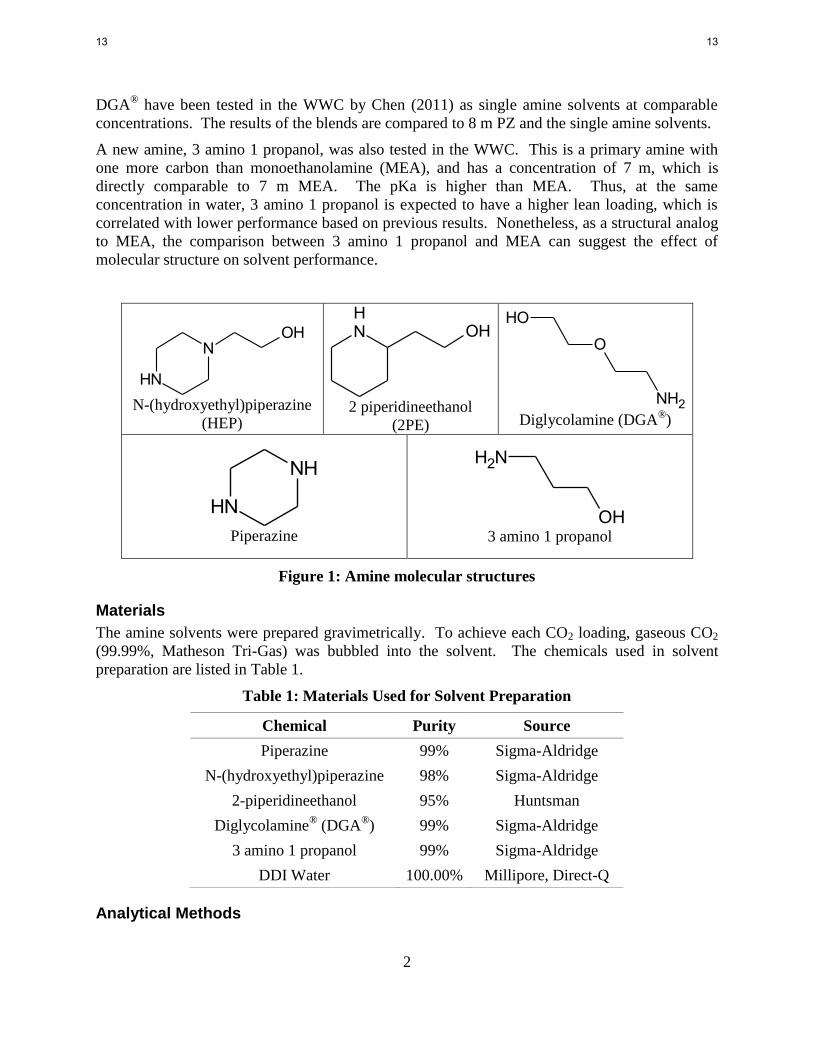
DGA® have been tested in the WWC by Chen (2011) as single amine solvents at comparable

concentrations. The results of the blends are compared to 8 m PZ and the single amine solvents.

A new amine, 3 amino 1 propanol, was also tested in the WWC. This is a primary amine with

one more carbon than monoethanolamine (MEA), and has a concentration of 7 m, which is

directly comparable to 7 m MEA. The pKa is higher than MEA. Thus, at the same

concentration in water, 3 amino 1 propanol is expected to have a higher lean loading, which is

correlated with lower performance based on previous results. Nonetheless, as a structural analog

to MEA, the comparison between 3 amino 1 propanol and MEA can suggest the effect of

molecular structure on solvent performance.

N

NH

OH

N-(hydroxyethyl)piperazine

(HEP)

NH

OH

2 piperidineethanol

(2PE)

OH

O

NH2 Diglycolamine (DGA

®)

NH

NH

Piperazine

NH2

OH 3 amino 1 propanol

Figure 1: Amine molecular structures

Materials

The amine solvents were prepared gravimetrically. To achieve each CO2 loading, gaseous CO2

(99.99%, Matheson Tri-Gas) was bubbled into the solvent. The chemicals used in solvent

preparation are listed in Table 1.

Table 1: Materials Used for Solvent Preparation

Chemical Purity Source

Piperazine 99% Sigma-Aldridge

N-(hydroxyethyl)piperazine 98% Sigma-Aldridge

2-piperidineethanol 95% Huntsman

Diglycolamine® (DGA

®) 99% Sigma-Aldridge

3 amino 1 propanol 99% Sigma-Aldridge

DDI Water 100.00% Millipore, Direct-Q

Analytical Methods

13 13

3

Liquid samples from each WWC experiment were analyzed for CO2 content and total alkalinity.

The total inorganic carbon (TIC) method was used to measure the total moles of CO2 per unit

mass of liquid sample. For each sample, TIC was performed in triplicate and the average value

was reported. The acid titration method was used to determine total alkalinity in each sample,

and the reported values are an average of triplicates. The apparatus and method for both TIC and

acid titration are identical to those used by Freeman (2011).

Safety considerations

The potential safety hazards in the operation of the WWC were discussed in the standard

operating procedure (SOP), which was included in a previous report (Rochelle et al., 2012).

Results and discussions

Absorption/desorption rates

Figure 2: Absorption rate of 6 m PZ/2 m HEP. Dashed lines: 8 m PZ at 40 ˚C (Dugas,

2009). Dotted lines: 7.7 m HEP at 40 ˚C (Chen, 2011).

The absorption rate of 6 m PZ/2 m HEP was measured in the WWC and represented as kg’,

which is the liquid side mass transfer coefficient. Absorption rate was measured at 20, 40, 60,

80, and 100 ˚C and variable CO2 loadings (Table 4). The measured results are plotted in Figure

2, and compared to 8 m PZ (Dugas, 2009) and 7.7 m HEP (Chen, 2011) at 40 ˚C. The absorption

rate of 6 m PZ/2 m HEP is similar to that of 8 m PZ at 40 ˚C, and is higher than 7.7 m HEP,

particularly at high loadings. The measured kg’ of the blend shows little temperature

dependence in the range of 20–60 ˚C. The kg’ at 100 ˚C is much lower than at other

temperatures, which suggests the diffusion of reactant and products becomes limiting relative to

1.E-07

1.E-06

100 1000 10000

k g' (

mo

l/P

a s

m2)

PCO2* @ 40 ˚C (Pa)

40 °C

80 °C

60 °C

100 °C

20 °C

8 m PZ @ 40 °C

7.7 m HEP @ 40 °C

14 14

4

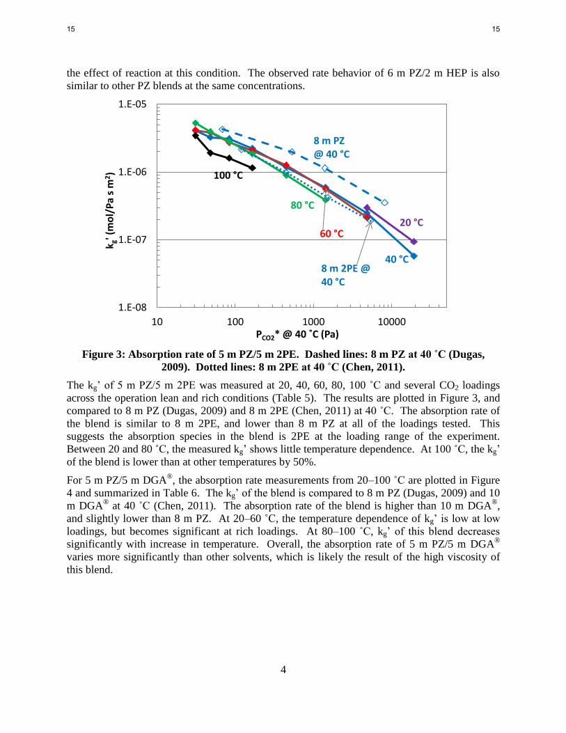
the effect of reaction at this condition. The observed rate behavior of 6 m PZ/2 m HEP is also

similar to other PZ blends at the same concentrations.

Figure 3: Absorption rate of 5 m PZ/5 m 2PE. Dashed lines: 8 m PZ at 40 ˚C (Dugas,

2009). Dotted lines: 8 m 2PE at 40 ˚C (Chen, 2011).

The kg’ of 5 m PZ/5 m 2PE was measured at 20, 40, 60, 80, 100 ˚C and several CO2 loadings

across the operation lean and rich conditions (Table 5). The results are plotted in Figure 3, and

compared to 8 m PZ (Dugas, 2009) and 8 m 2PE (Chen, 2011) at 40 ˚C. The absorption rate of

the blend is similar to 8 m 2PE, and lower than 8 m PZ at all of the loadings tested. This

suggests the absorption species in the blend is 2PE at the loading range of the experiment.

Between 20 and 80 ˚C, the measured kg’ shows little temperature dependence. At 100 ˚C, the kg’

of the blend is lower than at other temperatures by 50%.

For 5 m PZ/5 m DGA®, the absorption rate measurements from 20–100 ˚C are plotted in Figure

4 and summarized in Table 6. The kg’ of the blend is compared to 8 m PZ (Dugas, 2009) and 10

m DGA® at 40 ˚C (Chen, 2011). The absorption rate of the blend is higher than 10 m DGA

®,

and slightly lower than 8 m PZ. At 20–60 ˚C, the temperature dependence of kg’ is low at low

loadings, but becomes significant at rich loadings. At 80–100 ˚C, kg’ of this blend decreases

significantly with increase in temperature. Overall, the absorption rate of 5 m PZ/5 m DGA®

varies more significantly than other solvents, which is likely the result of the high viscosity of

this blend.

1.E-08

1.E-07

1.E-06

1.E-05

10 100 1000 10000

k g' (

mo

l/P

a s

m2)

PCO2* @ 40 ˚C (Pa)

40 °C

80 °C

60 °C

100 °C

20 °C

8 m PZ @ 40 °C

8 m 2PE @ 40 °C

15 15

5

Figure 4: Absorption rate of 5 m PZ/5 m DGA®

. Dashed lines: 8 m PZ at 40 ˚C (Dugas,

2009). Dotted lines: 10 m DGA®

at 40 ˚C (Chen, 2011).

Figure 5: Absorption rate of 7 m 3 amino 1 propanol. Dashed lines: 7 m MEA at 40 ˚C

(Dugas, 2009).

1.E-07

1.E-06

100 1000 10000

k g' (

mo

/Pa

s m

2)

PCO2* @ 40 ˚C (Pa)

40 °C

80 °C

60 °C 100 °C

20 °C

8 m PZ @ 40 °C

10 m DGA® @ 40 °C

1.E-08

1.E-07

1.E-06

1.E-05

10 100 1000 10000 100000

k g' (

mo

l/P

a s

m2)

PCO2* @ 40 ˚C (Pa)

40 °C

80 °C

60 °C

100 °C

20 °C

7 m MEA @ 40 °C

16 16

6

The absorption rate of 7 m 3 amino 1 propanol is measured at 20–100 ˚C (Table 7). The results

are plotted in Figure 5 and compared to 7 m MEA at 40 ˚C (Dugas, 2009). At 40 ˚C, the

absorption rate of 7 m 3 amino 1 propanol is slightly lower than 7 m MEA when compared at the

same PCO2*. The kg’ of 7 m 3 amino 1 propanol show little temperature dependence over the

entire range of temperature and CO2 loading tested. The experimentally measured kg’ is used to

predict the absorption performance of each solvent in an absorber. The parameter kg’avg is used

to represent an average absorption rate of a solvent at 40 ˚C between the top and bottom of an

optimized absorber (Equation 1).

⁄

( ) (

)

⁄

(1)

The kg’avg calculation assumes the absorber operates isothermally at 40 ˚C. Also, the

concentration profile of CO2 between the top and bottom of the absorber is assumed to vary

logarithmically. The calculated kg’avg of the new solvents is reported in Table 3.

CO2 solubility

The CO2 solubility of the new solvents is measured at low temperatures (20, 40, 60, 80, 100 ˚C)

and CO2 loadings across the standard lean and rich operation conditions. The experimentally

measured PCO2* results are used to calculate the parameters of a semi-empirical VLE model for

each solvent. The model is shown in Equation 2.

(

)

(2)

The parameters of the model for each solvent are reported in Table 2, together with the R2 value

of the regression. For all four solvents, the R2 value of the model is higher than 0.99, which

suggest the fit is acceptable. The model is used to interpolate VLE behavior of the solvent

between experimental conditions. Also, the model can be used quantify the temperature

behavior of CO2 VLE in each solvent, which is the heat of absorption of CO2.

17 17

7

Figure 6: CO2 solubility in 6 m PZ/2 m HEP. Diamond: WWC results. Solid lines:

empirical model (Table 2). Dashed line: empirical model of 8 m PZ (Xu, 2011).

The CO2 solubility of 6 m PZ/2 m HEP is measured at 20–100 ˚C, and the results are plotted in

Figure 6 and summarized in Table 4. The experimental values are compared to the results of the

semi-empirical model (Table 2) and the model result of 8 m PZ (Xu, 2011). The semi-empirical

model predicts the experimental data well across the range of conditions tested. At the same

CO2 loading, the blend has lower CO2 solubility than 8 m PZ, which corresponds to higher PCO2*.

The lower CO2 solubility is the result of the reduced alkalinity of the tertiary amine in HEP. The

CO2 solubility at 40 ˚C also suggest a reduced CO2 carrying capacity of the solvent in the

process, evident in the higher slope of the VLE curve.

The CO2 solubility result of 5 m PZ/5 m 2PE is plotted in Figure 7 and summarized in Table 5.

The results are compared against the semi-empirical model result of the blend and 8 m PZ. The

regressed model fits the experimental data well. The measured PCO2* is lower in the blend than 8

m PZ at the same CO2 loadings.

For 5 m PZ/5 m DGA®, the experimental results are plotted in Figure 8 and summarized in Table

6. The results are compared to the semi-empirical model result and 8 m PZ at 40 ˚C. The fit of

the semi-empirical model to the data is acceptable but not ideal. At low loadings, the shape of

the VLE curves suggests unrealistic physical behavior, though the statistical fit of the model is

high. This error in the model result is due to the simplistic form of the semi-empirical equation.

Thus, the model for this solvent ought to be used carefully at low loadings. More experimental

results at higher temperatures will be collected in the future using the total pressure apparatus,

which will improve the validity of the semi-empirical model for this blend.

10

100

1000

10000

100000

0.23 0.28 0.33 0.38

PC

O2*

(Pa)

CO2 loading (mol/mol alk)

40 °C

80 °C

60 °C

100 °C

20 °C

18 18

8

Figure 7: CO2 solubility in 5 m PZ/5 m 2PE. Diamond: WWC results. Solid lines:

empirical model (Table 2). Dashed line: empirical model of 8 m PZ (Xu, 2011).

Figure 8: CO2 solubility in 5 m PZ/5 m DGA®. Diamond: WWC results. Solid lines:

empirical model (Table 2). Dashed line: empirical model of 8 m PZ at 40 ˚C (Xu, 2011).

10

100

1000

10000

100000

0.17 0.22 0.27 0.32 0.37 0.42 0.47 0.52

PC

O2*

(Pa)


40 °C

80 °C

60 °C

100 °C

20 °C

100

1000

10000

100000

0.3 0.35 0.4 0.45

PC

O2*

(Pa)


40 °C

80 °C

60 °C

100 °C

20 °C

19 19

9

The CO2 solubility result of 7 m 3 amino 1 propanol is plotted in Figure 9 and summarized in

Table 7. The results are compared against the semi-empirical model predictions and the model

result of 8 m PZ and 40 ˚C. The semi-empirical model fits the experimental data well, with the

exception of the 40 ˚C point at the low loading condition. The poor fit of the low loading 40 ˚C

point is due to the quality of experimental data, which is close to the low measurement limit of

the WWC apparatus. The PCO2* in the 3 amino 1 propanol is lower than 7 m MEA at the lower

loadings in the experimental range. The observed increase in CO2 solubility can be explained by

the higher pKa of 3 amino 1 propanol, which results in higher chemical attraction to CO2.

Figure 9: CO2 solubility in 7 m 3 amino 1 propanol. Diamond: WWC results. Solid lines:

empirical model (Table 2). Dashed line: empirical model of 7 m MEA at 40 ˚C (Xu, 2011).

Table 2: Parameters of semi-empirical VLE model (Equation 2) of the screened solvents

Solvent a b c d e f R2

6 m PZ/2 m HEP 0 3462.9 219.4 -328.9 -86106.6 145191.2 0.9997

5 m PZ/5 m 2PE 18.7 -4520.5 130.9 -206.2 -44550.1 77422.5 0.992

5 m PZ/5 m DGA®

0 9957.7 195.1 -242.0 -111006 152194 0.9994

7 m 3 amino 1

propanol 53.5 -14756.1 -35.5 0 0 22721.6 0.995

The semi-empirical model for each solvent (Table 2) is used to estimate the standard operation

lean and rich loadings, which are assumed to correspond to PCO2* at 0.5 and 5 kPa at 40 ˚C. The

CO2 solubility in each solvent determines the energy performance of the solvent in a real

absorption process. This energy performance is represented partly in the CO2 carrying capacity

of the solvent, which is calculated using Equation 3.

10

100

1000

10000

100000

0.3 0.35 0.4 0.45 0.5 0.55 0.6

PC

O2*

(Pa)

CO2 loading (mol/mol alkalinity)

40 °C

80 °C

60 °C

100 °C

20 °C 7 m MEA @ 40 °C

20 20

10

(3)

Solvents with higher capacity absorb more CO2 in the absorber per unit mass of the solvent,

which reduces the energy required to cycle and heat the solvent in the process. Since the

calculation of capacity requires the difference between the operation lean and rich loadings of the

solvent, its value is closely associated with the shape of the VLE curve at 40 ˚C.

The semi-empirical model of each solvent is also used to estimate the heat of absorption of CO2,

which is calculated using Equation 4.

(

( ⁄ ))

(4)

The heat of absorption of CO2 in a solvent can be observed as the temperature dependence of the

CO2 VLE.

The calculated capacity and heat of absorption of CO2 for the new solvents are summarized in

Table 3, and compared with the results of 8 m PZ, 7 m MEA, and 5 m PZ/5 m MDEA. The

capacity of 6 m PZ/2 m HEP is about 25% lower than that of 8 m PZ, though the two solvents

have the same concentration of total alkalinity. 5 m PZ/5 m 2PE has capacity about 25% lower

than 8 m PZ, due to the lower concentration of total alkalinity in the solvent. 5 m PZ/5 m DGA®

has much lower capacity than 8 m PZ, by about 45%. Comparing the PZ/2PE and PZ/DGA®

blends to 5 m PZ/5 m MDEA, which has the same concentration in alkalinity, the new blends

have lower capacity than the MDEA blend. This result suggests that PZ blends with tertiary

amines have better capacity than primary and hindered amine blends when compared at the 5 m

PZ/5 m amine condition. The new primary amine solvent, 7 m 3 amino 1 propanol, has low

capacity, which is about 50% less than 7 m MEA and much lower than 8 m PZ.

Table 3: Predicted performance parameters of screened solvents

Con kg'avg @ 40 ˚C Capacity lean/rich

-Habs @

PCO2* =1.5

kPa

(m) Х107 mol/Pa s m

2 mol/kg solv mol/mol alk kJ/mol

PZ / HEP 6 / 2 8.66 0.66 0.287 / 0.360 76

PZ / 2PE 5 / 5 4.20 0.67 0.396 / 0.488 75

PZ / DGA®

5 / 5 6.74 0.48 0.370 / 0.433 83

PZ 8 8.50 0.86 0.31/0.40 67

PZ / MDEA 5 / 5 8.34 0.98 0.21/0.35 69

3 amino 1

propanol 7 2.52 0.27 0.485 / 0.544 73

MEA 7 4.35 0.50 0.434 / 0.535 73

The heat of absorption of 6 m PZ/2 m HEP and 5 m PZ/5 m 2PE about 75 kJ/mol, which is

competitive with 7 m MEA and higher than 8 m PZ. The heat of absorption of 5 m PZ/5 m

DGA®

is calculated to be 83 kJ/mol, which is much higher than 7 m MEA and 8 m PZ. The high

heat of absorption of this blend can be explained by the presence of DGA®, which has high heat

of absorption. Also, the value calculated is potentially an over-prediction as result of the

21 21

11

unrealistic trends observed in the semi-empirical model of this solvent. The heat of absorption of

7 m 3 amino 1 propanol is similar to that of 7 m MEA.

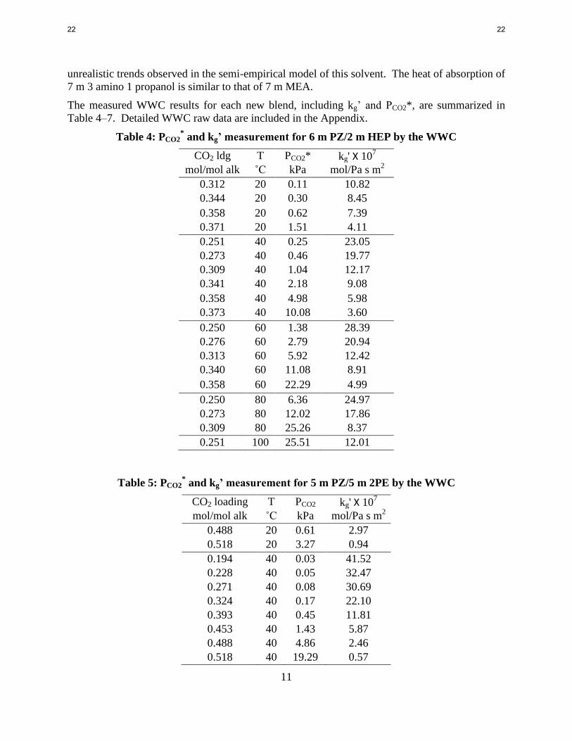
The measured WWC results for each new blend, including kg’ and PCO2*, are summarized in

Table 4–7. Detailed WWC raw data are included in the Appendix.

Table 4: PCO2* and kg’ measurement for 6 m PZ/2 m HEP by the WWC

CO2 ldg T PCO2* kg' Х 107

mol/mol alk ˚C kPa mol/Pa s m2

0.312 20 0.11 10.82

0.344 20 0.30 8.45

0.358 20 0.62 7.39

0.371 20 1.51 4.11

0.251 40 0.25 23.05

0.273 40 0.46 19.77

0.309 40 1.04 12.17

0.341 40 2.18 9.08

0.358 40 4.98 5.98

0.373 40 10.08 3.60

0.250 60 1.38 28.39

0.276 60 2.79 20.94

0.313 60 5.92 12.42

0.340 60 11.08 8.91

0.358 60 22.29 4.99

0.250 80 6.36 24.97

0.273 80 12.02 17.86

0.309 80 25.26 8.37

0.251 100 25.51 12.01

Table 5: PCO2* and kg’ measurement for 5 m PZ/5 m 2PE by the WWC

CO2 loading T PCO2 kg' Х 107


0.488 20 0.61 2.97

0.518 20 3.27 0.94

0.194 40 0.03 41.52

0.228 40 0.05 32.47

0.271 40 0.08 30.69

0.324 40 0.17 22.10

0.393 40 0.45 11.81

0.453 40 1.43 5.87

0.488 40 4.86 2.46

0.518 40 19.29 0.57

22 22

12

0.194 60 0.24 41.01

0.228 60 0.37 38.60

0.271 60 0.61 27.20

0.324 60 1.19 20.90

0.393 60 3.23 12.60

0.453 60 8.75 5.62

0.488 60 25.22 2.12

0.194 80 1.31 52.80

0.228 80 2.46 39.23

0.271 80 3.70 27.95

0.324 80 7.71 18.57

0.393 80 19.14 8.93

0.453 80 39.05 3.86

0.194 100 7.54 34.55

0.228 100 11.98 19.10

0.271 100 16.84 16.00

0.324 100 30.22 11.50

Table 6: PCO2* and kg’ measurement for 5 m PZ/5 m DGA

® by the WWC

CO2 ldg T PCO2* kg' Х 107


0.418 20 0.21 7.99

0.437 20 0.82 3.92

0.457 20 2.81 2.08

0.321 40 0.29 17.59

0.369 40 0.66 13.36

0.418 40 2.04 7.65

0.437 40 7.05 3.29

0.457 40 25.51 1.12

0.321 60 2.21 18.20

0.369 60 5.00 11.25

0.418 60 11.40 6.60

0.437 60 44.80 1.97

0.321 80 10.25 13.56

0.369 80 24.75 6.55

0.418 80 69.17 2.61

0.321 100 51.74 6.71

Table 7: PCO2* and kg’ measurement for 7 m 3 amino 1 propanol by the WWC

CO2 loading T kg' Х 107 PCO2*

mol/mol alk ˚C mol/Pa s m2 kPa

0.553 20 1.18 1.75

23 23

13

0.586 20 0.60 6.34

0.325 40 23.20 0.03

0.385 40 14.15 0.03

0.472 40 7.84 0.25

0.508 40 3.58 1.06

0.553 40 1.37 8.66

0.586 40 0.32 39.95

0.325 60 23.10 0.14

0.385 60 17.10 0.30

0.472 60 8.87 1.77

0.508 60 4.28 7.12

0.553 60 1.22 31.08

0.325 80 27.20 0.92

0.385 80 19.41 2.11

0.472 80 9.43 10.11

0.508 80 3.36 31.28

0.325 100 24.90 6.56

0.385 100 16.40 12.12

0.472 100 5.99 42.06

Conclusions

6 m PZ/2 m HEP has an absorption rate similar to 8 m PZ. The capacity of the blend is 0.66

mol/kg solvent, which is about 25% less than 8 m PZ. The heat of absorption is 76 kJ/mol,

which is competitive with 7 m MEA and higher than 8 m PZ.

The absorption rate of 5 m PZ/5 m 2PE is about 50% lower than 8 m PZ. The capacity of this

blend is 0.67 mol/kg solvent, about 25% less than 8 m PZ. The heat of absorption of this solvent

is 75 kJ/mol, which is competitive with 7 m MEA and higher than 8 m PZ.

The blend of 5 m PZ/5 m DGA® has a moderate absorption rate, about 20% less than 8 m PZ.

The capacity of this blend is also low, at 0.48 mol/kg solvent, which is about 40% less than 8 m

PZ. The heat of absorption is high at 83 kJ/mol. However, there is likely a slight over-

prediction in the calculated value of heat of absorption due to observed error in the analysis.

The new primary amine solvent 7 m 3 amino 1 propanol is not competitive against 7 m MEA.

The absorption rate and capacity of this solvent are both about 50% of 7 m MEA. Only the heat

of absorption is about the same as 7 m MEA.

Future Work

During the next quarter, new amines including two primary amines and three secondary amines

will be tested in the WWC.

24 24

14

References

Chen X. Carbon dioxide thermodynamics, kinetics, and mass transfer in aqueous piperazine

derivatives and other amines. The University of Texas at Austin. Ph.D. Dissertation. 2011.

Dugas RE. Carbon dioxide absorption, desorption, and diffusion in aqueous piperazine and

monoethanolamine. The University of Texas at Austin. Ph.D. Dissertation. 2009.

Freeman SA. Thermal degradation and oxidation of aqueous piperazine for carbon dioxide

capture. The University of Texas at Austin. Ph.D. Dissertation. 2011.

Rochelle GT et al. "CO2 Capture by Aqueous Absorption, Second Quarterly Progress Report

2012." Luminant Carbon Management Program. The University of Texas at Austin. 2012.

Xu Q. Thermodynamics of CO2 loaded aqueous amines. The University of Texas at Austin.

Ph.D. Dissertation. 2011.

25 25

1

Aqueous piperazine/aminoethylpiperazine for CO2 Capture


by Yang Du




July 31, 2013

Abstract

A model accurately predicting thermodynamic and kinetic properties for CO2 absorption in

aqueous amine solutions is essential for simulation and design of such a CO2 capture process.

Last quarter, a rigorous thermodynamic model for PZ-AEP-H2O-CO2 was developed based on

the Independence model for PZ-H2O-CO2 in Aspen Plus® using the electrolyte-Nonrandom Two-

Liquid (e-NRTL) activity coefficient model. This quarter, qualitative H1 and C

13 NMR

measurement was used to correct the speciation prediction by this model. Model parameters

were carefully selected in the regressions of the vapor-liquid equilibrium (VLE) data for AEP-

H2O-CO2 and PZ-AEP-H2O-CO2 to assure the correct speciation prediction by this model. The

speciation and heat of absorption for AEP-H2O-CO2 and PZ-AEP-H2O-CO2 were also predicted

using this updated model. At 40 °C the heat of absorption of 6 m AEP is about 60–90 kJ/mol

CO2 at operation loading range (0.27–0.33) and the heat of absorption of 5 m PZ/2 m AEP is

about 60–80 kJ/mol CO2 at operation loading range (0.3–0.38).

In addition, pulsed field gradient (PFG) spin echo (SE) - H1 NMR was used this quarter to

measure the self-diffusion coefficient of unloaded aqueous AEP solutions. The diffusivity of

AEP solutions was found to be inversely proportional to its viscosity with a power of 0.6.

Introduction

Amine scrubbing has shown the most promise for effective capture of CO2 from coal-fired flue

gas. Piperazine/N-(2-aminoethyl)piperazine (PZ/AEP) was investigated in this study as a novel

solvent for CO2 capture. In previous reports, we have confirmed that PZ/AEP has a larger solid

solubility window than concentrated PZ, slightly lower CO2 absorption capacity, but comparable

resistance to degradation, CO2 absorption rate, and viscosity, which indicates PZ/AEP is a

superior solvent for CO2 capture by absorption/stripping.

To properly simulate and design the CO2 capture process using PZ/AEP, it is necessary to

develop a rigorous thermodynamic model which can accurately predict the thermodynamic

properties, specifically vapor-liquid equilibrium (VLE), calorimetric properties, and chemical

reaction equilibrium.

Last quarter, a rigorous thermodynamic model was developed for PZ-AEP-H2O-CO2 in Aspen

Plus® using the electrolyte-Nonrandom Two-Liquid (e-NRTL) activity coefficient model, based

on the Independence model for concentrated PZ developed by Frailie (Rochelle, 2012). This

26 26

2

model can accurately predict VLE of 6 m AEP and 5 m PZ/2 m AEP at practical loading and

temperature range, but the predicted speciation was not consistent with quantitative NMR

measurement.

This quarter, model parameters were carefully selected in the regressions of the vapor-liquid

equilibrium (VLE) data for AEP-H2O-CO2 and PZ-AEP-H2O-CO2 to assure the correct

speciation prediction by this model. The speciation and heat of absorption for AEP-H2O-CO2

and PZ-AEP-H2O-CO2 were also predicted using this updated model. In addition, pulsed field

gradient (PFG) spin echo (SE) - H1 NMR was used to measure the self-diffusion coefficient of

unloaded aqueous AEP solutions.

Experimental Methods

Quantitative NMR measurement

H-NMR and C13

-NMR measurements were conducted for loaded 6 m AEP and 5 m PZ/2 m AEP.

All solutions were prepared gravimetrically from ultra pure deionized water. Amine solutions

were loaded with CO2 by slowly sparging C13

CO2. Experimental apparatus, procedure, and

analytical methods were described in detail by Hilliard (2008).

Pulsed field gradient (PFG) spin echo (SE) - H1 NMR

PFG-SE nuclear magnetic resonance provides a convenient and noninvasive means for

measuring self-diffusion. In this method, the attenuation of a spin-echo signal resulting from the

dephasing of the nuclear spins due to the combination of the translational motion of the spins and

the imposition of spatially well-defined gradient pulses is used to measure motion. The spin

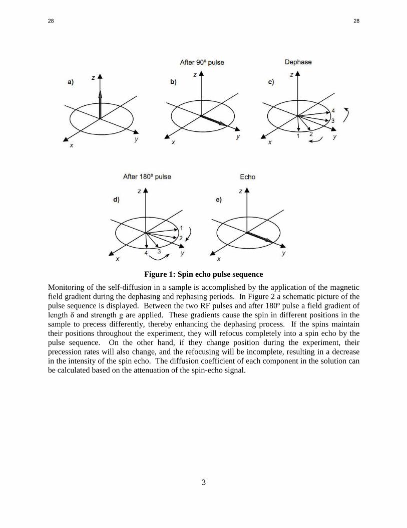
echo sequence is illustrated in Figure 1. Initially the magnetization is parallel to the external

field (Figure 1a). A 90º pulse is then applied along the x direction so that the net magnetization

now lies in the xy plane, in the y axis (Figure 1b). During the period of time following the RF

pulse, spins begin to dephase due to their unique gyromagnetic ratio, as shown in Figure 1c. At a

time τ a 180º pulse is applied along the y direction as shown in Figure 1d. The spins are

therefore rotated by 180º around the y axis thereby remaining in the xy plane. As a result of the

inverted relative positions, and because each spin continues to precess with its former frequency,

all spins will be perfectly reclustered at time 2τ forming an echo (Figure 1e).

27 27

3

Figure 1: Spin echo pulse sequence

Monitoring of the self-diffusion in a sample is accomplished by the application of the magnetic

field gradient during the dephasing and rephasing periods. In Figure 2 a schematic picture of the

pulse sequence is displayed. Between the two RF pulses and after 180º pulse a field gradient of

length δ and strength g are applied. These gradients cause the spin in different positions in the

sample to precess differently, thereby enhancing the dephasing process. If the spins maintain

their positions throughout the experiment, they will refocus completely into a spin echo by the

pulse sequence. On the other hand, if they change position during the experiment, their

precession rates will also change, and the refocusing will be incomplete, resulting in a decrease

in the intensity of the spin echo. The diffusion coefficient of each component in the solution can

be calculated based on the attenuation of the spin-echo signal.

28 28

4

Figure 2: A schematic representation of the PFG-SE process

Safety Considerations

1,4-Dioxane is a very dangerous substance, causing damage to the central nervous system, liver,

and kidneys. Also, 1,4-dioxane is highly flammable and potentially explosive if not stored

properly. For safety purposes, the 1,4-Dioxane is stored in the “flammables” cabinet, and all

work with it is done with safety glasses, chemical resistant gloves, and a lab coat.

Results and discussion

Quantitative NMR measurement

For the identification of NMR peaks for reactive solution we need to figure out what kind of

species may exist in the solution according to reaction mechanism. For the loaded AEP system,

the following 6 species may be the dominant species in the solution:

AEP AEPH+ AEP(H

+)2

N

NH

NH2 N

NH

NH3+

N

NH2+

NH3+

29 29

5

NN

NH

R

R

AEPCOO- HAEPCOO AEP(COO

-)2

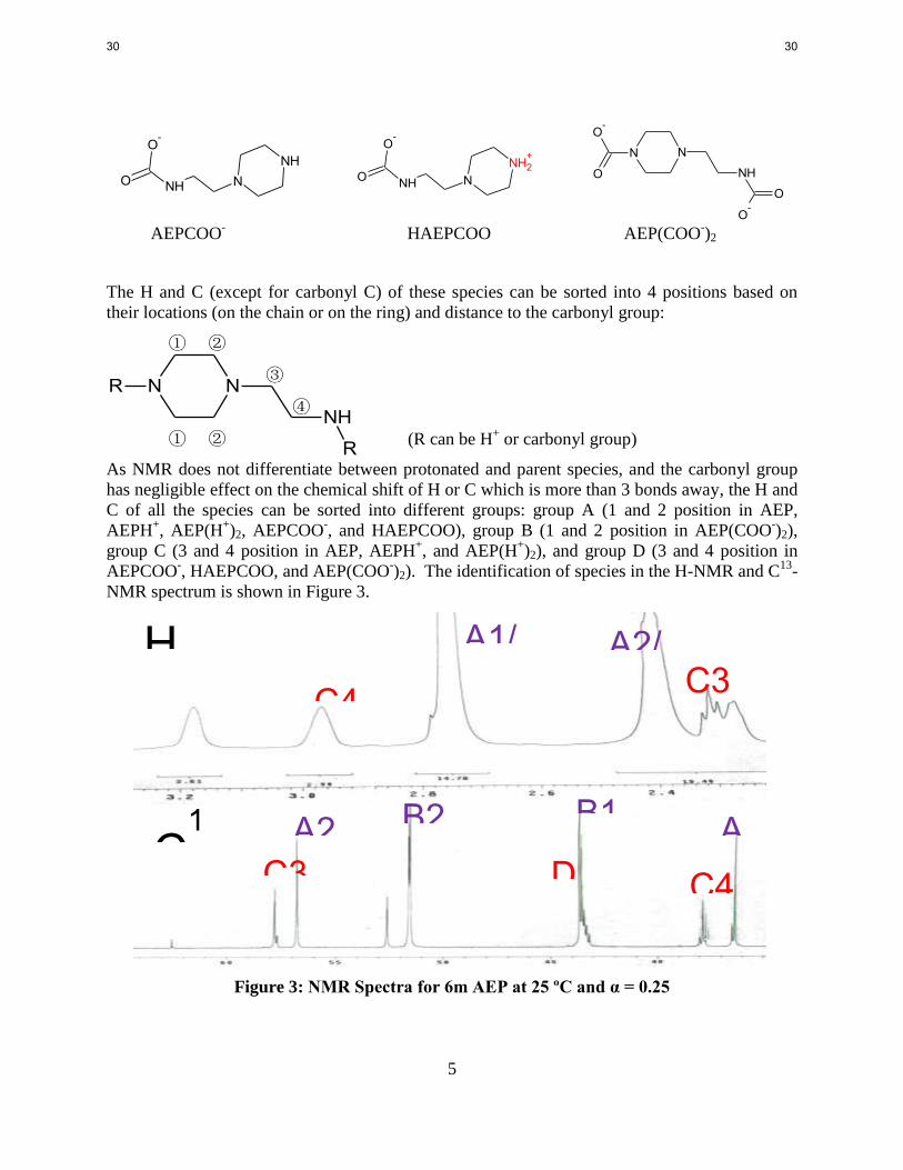
The H and C (except for carbonyl C) of these species can be sorted into 4 positions based on

their locations (on the chain or on the ring) and distance to the carbonyl group:

① ②

③

④

① ② (R can be H+ or carbonyl group)

As NMR does not differentiate between protonated and parent species, and the carbonyl group

has negligible effect on the chemical shift of H or C which is more than 3 bonds away, the H and

C of all the species can be sorted into different groups: group A (1 and 2 position in AEP,

AEPH+, AEP(H

+)2, AEPCOO

-, and HAEPCOO), group B (1 and 2 position in AEP(COO

-)2),

group C (3 and 4 position in AEP, AEPH+, and AEP(H

+)2), and group D (3 and 4 position in

AEPCOO-, HAEPCOO, and AEP(COO

-)2). The identification of species in the H-NMR and C

13-

NMR spectrum is shown in Figure 3.

Figure 3: NMR Spectra for 6m AEP at 25 ºC and α = 0.25

A1/B1

A2/B2

D4

C4 C3 D3

C3

A2

D3

B2 B1

C4

A1 D

4

H1

C1

3

NNH

NHO

O-NN

NH

O

O-

O

O-

NNH2

+

NHO

O-

30 30

6

The NMR spectra for 6 m AEP at α = 0.35, and for 5 m PZ/2 m AEP at α = 0.25 and 0.35 are

also identified but not shown here. Based on the peak area of each group their concentration in

the solutions can be calculated. The results will be shown later.

Diffusivity measurement

The self-diffusion coefficient of unloaded aqueous AEP solutions with variable concentration

was measured by pulsed field gradient (PFG) spin echo (SE) - H1 NMR. The diffusivity of AEP

solutions was found to be inversely proportional to its viscosity with a power of 0.6, as shown in

Figure 4.

Figure 4: Diffusivity for AEP-H2O with different viscosity at 25 ºC

Model correction based on quantitative NMR measurement

The model developed last quarter accurately predicts vapor-liquid equilibrium (VLE) of 6 m

AEP and 5 m PZ/2 m AEP at practical loading and temperature range, but the predicted

speciation was not consistent with quantitative NMR measurement. To correct this issue, model

parameters were carefully selected this quarter in the regressions of the VLE data for AEP-H2O-

CO2 and PZ-AEP-H2O-CO2 to assure the correct speciation prediction by this model. After

regression, the speciation prediction by the model is consistent with the NMR measurement

(Figure 5 and 6).

0.2 m — 3 m AEP

31 31

7

Figure 5: Speciation validation for 6 m AEP-CO2-H2O

NNH

NHO

O-

NNH2

+

NHO

O-

NNNH

O

O-

O

O-

N

NH

NH2 N

NH

NH3+

N

NH2+

NH3+

Points: H-NMR result Lines: model prediction

32 32

8

Figure 6: Speciation validation for 5 m PZ/2 m AEP

Vapor-liquid equilibrium prediction by the updated model

The vapor-liquid equilibrium (VLE) of 6 m AEP is predicted well by the model (Figure 7). The

updated regressed parameters and standard error are summarized in Table 1.

Points: H-NMR result Lines: model prediction

33 33

9

Figure 7: Experimental measurement (points) (Chen, 2011) and Aspen Plus® predictions

(lines) for VLE of loaded 6 m AEP solution between 40 °C and 100 °C

Table 1: the regressed parameters and standard error

Parameter Comp. i Comp. j Regressed value Standard error

Δf Gi∞, aq

AEPCOO-

——

-97.6 0.73

AEPCOO-2 -450 0.96

Δf Hi∞, aq

AEPCOO- -511 2.82

AEPCOO-2 -966 12.7

GMELCC/1

H2O (AEPH+2,

HCO3-) 8.95 0.11

H2O (AEPH+2,

AEPCOO-) 9.11 0.22

Also, after regression, the VLE of 5 m PZ/2 m AEP is predicted well by the model (Figure 8),

especially at the normal operational conditions (rich loading at low T, and lean loading at high T).

The updated regressed parameters and standard error are summarized in Table 2.

34 34

10

Figure 8: Comparison of Aspen Plus® predictions (lines) and experimental data (points) for

loaded 6 m AEP between 40 °C and 160 °C

Table 2: Regressed parameters and standard error

Parameter Comp. i Comp. j Value Standard deviation

GMELCC/1 (PZH+,AEPCOO-) H2O -6.3 19.1 GMELCC/1 (AEPH+2,PZCOO-) H2O -4.4 21.5 GMELCC/1 (AEPH+2,PZCOO-2) H2O -4.1 18.0 GMELCC/1 (AEPH+2,PZCOO-2) HPZCOO -6.4 83.2 GMELCC/1 (AEPH+2,AEPCOO-) HPZCOO -6.4 10.5

GMELCC/1 (PZH+,AEPCOO-) HPZCOO -7 0

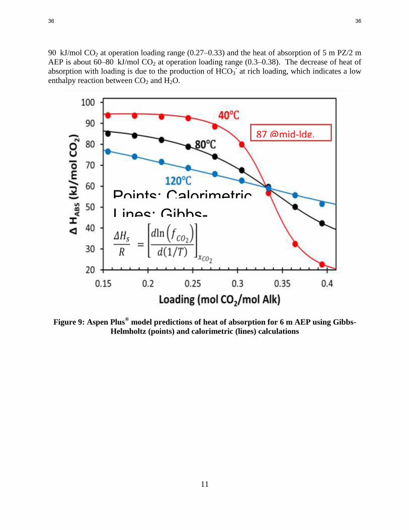
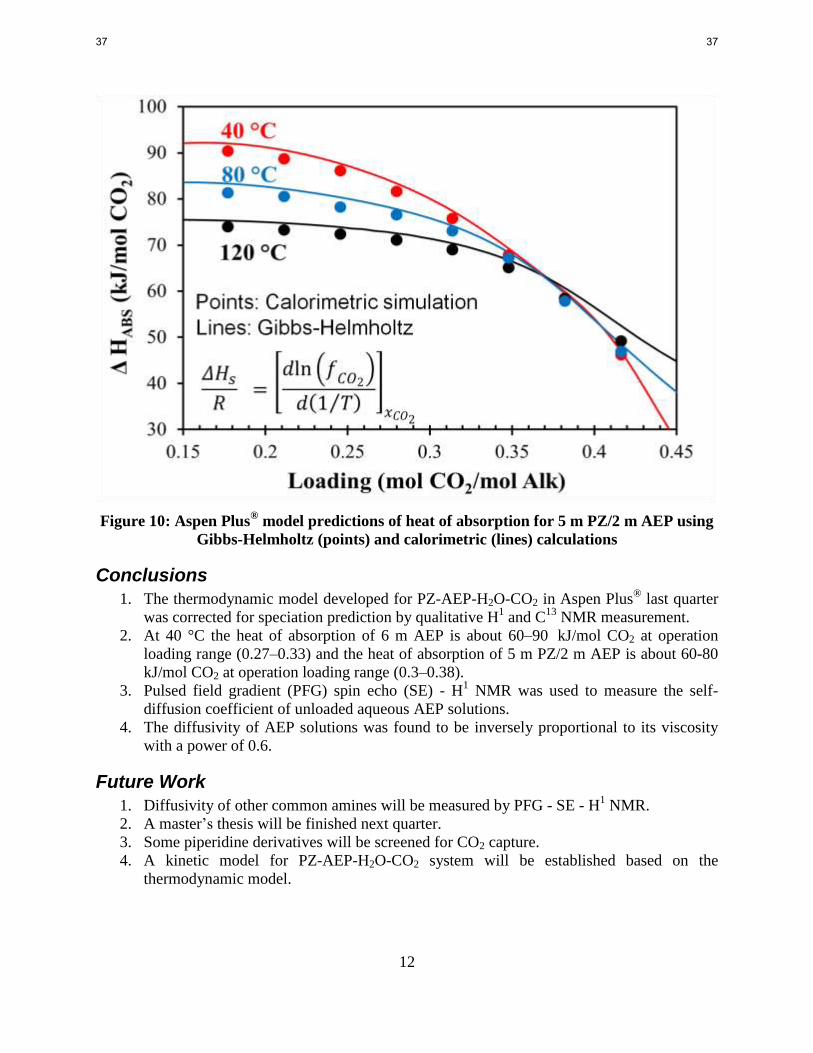
Heat of absorption prediction by the updated model

Heat of absorption predictions in Aspen Plus® can be calculated using the calorimetric method

and the Gibbs-Helmholtz equation. In the updated model, these two methods give more

consistent results of Habs-CO2 than the last version of the model. The large discrepancy of

prediction between these two methods in the last version of the model is thought to be due to the

over-adjustment of binary parameters. The prediction of heat of absorption for AEP and

PZ/AEP is shown in Figures 9 and 10. At 40 °C the heat of absorption of 6 m AEP is about 60–

Solid points: WWC (Li Le); Open points: High TP Autoclave Lines: Aspen model

35 35

11

90 kJ/mol CO2 at operation loading range (0.27–0.33) and the heat of absorption of 5 m PZ/2 m

AEP is about 60–80 kJ/mol CO2 at operation loading range (0.3–0.38). The decrease of heat of

absorption with loading is due to the production of HCO3- at rich loading, which indicates a low

enthalpy reaction between CO2 and H2O.

Figure 9: Aspen Plus® model predictions of heat of absorption for 6 m AEP using Gibbs-

Helmholtz (points) and calorimetric (lines) calculations

Points: Calorimetric simulation Lines: Gibbs-Helmholtz

87 @mid-ldg, 40C

36 36

12

Figure 10: Aspen Plus® model predictions of heat of absorption for 5 m PZ/2 m AEP using

Gibbs-Helmholtz (points) and calorimetric (lines) calculations

Conclusions

1. The thermodynamic model developed for PZ-AEP-H2O-CO2 in Aspen Plus® last quarter

was corrected for speciation prediction by qualitative H1 and C

13 NMR measurement.

2. At 40 °C the heat of absorption of 6 m AEP is about 60–90 kJ/mol CO2 at operation

loading range (0.27–0.33) and the heat of absorption of 5 m PZ/2 m AEP is about 60-80 kJ/mol CO2 at operation loading range (0.3–0.38).

3. Pulsed field gradient (PFG) spin echo (SE) - H1 NMR was used to measure the self-

diffusion coefficient of unloaded aqueous AEP solutions.

4. The diffusivity of AEP solutions was found to be inversely proportional to its viscosity

with a power of 0.6.

Future Work

1. Diffusivity of other common amines will be measured by PFG - SE - H1 NMR.

2. A master’s thesis will be finished next quarter.

3. Some piperidine derivatives will be screened for CO2 capture.

4. A kinetic model for PZ-AEP-H2O-CO2 system will be established based on the

thermodynamic model.

37 37

13

References

Chen X. Carbon dioxide thermodynamics, kinetics, and mass transfer in aqueous piperazine

derivatives and other amines. The University of Texas at Austin. Ph.D. Dissertation. 2011.

Hilliard MD. A Predictive Thermodynamic Model for an Aqueous Blend of Potassium

Carbonate, Piperazine, and Monoethanolamine for Carbon Dioxide Capture from Flue Gas.

The University of Texas at Austin. Ph.D. Dissertation. 2008.

Rochelle GT, et al. "CO2 Capture by Aqueous Absorption, Third Quarterly Progress Report


38 38

1

Process Economics for 8 m PZ


by Peter Frailie


Texas Carbon Management Program


July 31, 2013

Abstract

The goal of this study is to evaluate the performance of an absorber/stripper operation that

utilizes MDEA/PZ. Before analyzing unit operations and process configurations,

thermodynamic, hydraulic, and kinetic properties for the blended amine must be satisfactorily

regressed in Aspen Plus®

. The approach used in this study is first to construct separate MDEA

and PZ models that can later be reconciled via cross parameters to model MDEA/PZ accurately.

During the past quarter a base-case absorption/stripping process was designed and evaluated

using concentrated PZ. A techno-economic analysis was also performed to determine the effects

of process modifications on the ultimate cost of CO2 capture. Emphasis was placed on the

relative contributions of major process units to the final cost. All results were generated using

the Independence model. The goal for the next quarter is to finish the techno-economic analysis,

which will complete the work for this project.

Introduction

The removal of CO2 from process gases using alkanolamine absorption/stripping has been

extensively studied for several solvents and solvent blends. An advantage of using blends is that

the addition of certain solvents can enhance the overall performance of the CO2 removal system.

A disadvantage of using blends is that they are very complex compared to a single solvent, thus

making them much more difficult to model.

This study will focus on a blended amine solvent containing piperazine (PZ) and

methyldiethanolamine (MDEA). Previous studies have shown that this particular blend has the

potential to combine the high capacity of MDEA with the attractive kinetics of PZ (Bishnoi,

2000). These studies have supplied a rudimentary Aspen Plus®-based model for an absorber

with MDEA/PZ. This previous work recommended that more kinetic and thermodynamic data

should be acquired for the MDEA/PZ blend before the model can be significantly improved.

Three researchers in the Rochelle lab have been acquiring these data, which are being

incorporated into the model. One of the major goals of this study will be to improve the supplied

Aspen Plus® absorber model with up-to-date thermodynamic and kinetic data. Another major

goal will be to make improvements to the MDEA and PZ thermodynamic models, which should

simplify the construction of the blended amine model.

39 39

2

Methods

During the past quarter the techno-economic model was completed and used to evaluate the cost

effectiveness of the base-case absorption/stripping process described in the previous report.

Calculating cost of CO2 capture

The purchased equipment cost (PEC) for each process unit was calculated using the pricing

methods described in the 2013 Q1 Report and Aspen Plus® results. Over 80% of the PEC can be

attributed to four process units: (1) absorber, (2) reboiler, (3) main cross exchanger, and (4)

compressor. Other process units such as the stripper, pumps, trim cooler, and blower

cumulatively account for a significant cost, but they do not represent a significant opportunity for

design improvement and cost reduction.

In order to compare the effects of process conditions on CAPEX and OPEX, both expenses must

be expressed in dollars per metric ton of CO2 captured. The PEC was converted to these units

using Equation 1.

(1)

In Equation 1 converts the PEC to a total capital requirement (TCR) and annualizes the cost.

Literature values for range from as low as 3 to as high as 10, depending on the process unit in

question. This study will assume a constant value of 5 for for the entire process. The

annualizing factor, , takes into account return on investment (10%), taxes (35% of return on

investment), depreciation (3–10%, depending on plant lifetime), and maintenance (2–3%). If it

is assumed that the plant lifetime is 20 years and the value of the plant at the end of year 20 is $0,

is about 0.2. When multiplied together and yield a factor of 1, meaning that the CAPEX

contribution to the cost of CO2 capture can be calculated by dividing the PEC by the total metric

tons of CO2 captured per year by the process. The number of metric tons of CO2 captured per

year was calculated using the flue gas of a 550 MWe power plant and assuming a 90% capture

rate and 85% annual capacity.

The OPEX was expressed in dollars per metric ton of CO2 captured by calculating the

opportunity cost associated with operating each process unit. Every kWh used to overcome

pressure drop in columns and exchangers, operate the multi-stage compressor, and heat the

reboiler is a kWh of electricity that could not be sold to the market. The cost of electricity

(COE) was initially assumed to be $0.10 per kWh, and the sensitivity of the final solution to this

assumption was tested. The pump work was directly converted to kWh using Aspen Plus®

predictions. Reboiler duty was first converted from a heat duty to an equivalent work in the units

of kJ per mole of CO2 captured using Equation 2.

reboilersn

i i

kiieq

KT

TKTQCOmolkJW

1

sin2

5

575.0/ (2)

In Equation 2, Qi is the reboiler duty, Ti is the reboiler temperature, Tsink is 313K, 0.75 is the

steam turbine efficiency, and 5K is the temperature approach on the reboiler. This is the same

equation commonly used in this study to calculate the equivalent work of the reboiler.

yearpercapturedMTTotal

PECCOMT

2/$

40 40

3

Compressor work was calculated as a function of inlet CO2 pressure according to Equations 3

and 4.

atmP

atmPCOmolkJW in

in

comps 5.4096.4148

log572.4/ 2

(3)

atmP

atmPCOmolkJW in

in

comps 5.4181.2148

log023.4/ 2

(4)

For all cases the CO2 was compressed to 150 bar.

Results and Discussion

Table 1 reports the total cost of CO2 capture for several lean loadings, liquid rates, and absorber

configurations for 8 m PZ.

Table 1: Total cost of CO2 capture in USD per metric ton captured for several lean

loadings, liquid rates, and absorber configurations for 8 m PZ.

Lean Loading

(mol CO2/ mol alk)

1.1 x L/Gmin 1.2 x L/Gmin 1.3 x L/Gmin

IO IC PA IC IO IC PA IC IO IC PA IC

0.2 N/A 43.56 44.41 44.62 45.59 N/A

0.23 44.22 43.70 44.90 44.78 46.22 46.00

0.26 45.67 44.71 46.85 45.94 47.95 46.90

0.29 47.24 46.85 49.13 48.35 50.44 49.40

0.32 50.64 50.61 52.00 52.14 55.00 53.68

0.35 60.04 N/A 60.82 60.73 64.92 N/A

It should be noted that the prices in Table 1 do not include the cost of transportation, storage, and

monitoring (TS&M). A typical cost of TS&M is around $15 per metric ton of CO2. The

intercooling configurations are abbreviated IO IC (in-and-out intercooling) and PA IC (pump-

around intercooling), and they are described in detail in the 2013 Q1 Report (Rochelle et al.,

2013). For all liquid rates and intercooling configurations the cost of CO2 capture increases as

lean loading increases. For most liquid rates and lean loadings the pump-around intercooling is

slightly less expensive than in-and-out intercooling, though the difference in cost is never greater

than $1.32 per metric ton of CO2. As the liquid rate increases the cost of capture increases for all

lean loadings and configurations.

Figure 1 shows the minimum liquid flowrate in kg per second, CAPEX, and OPEX as a function

of lean loading for the configuration with a liquid flowrate that is 1.2 times the minimum and

pump-around intercooling. As the lean loading increases from 0.2 to 0.35 the minimum liquid

flowrate increases 236%. This is primarily due to the relatively small change in the rich loading

across the lean loading range. The rich loading is set by the temperature of the liquid at the

bottom of the absorber. For all cases this temperature is relatively close to the inlet gas

temperature (313K) because (1) at a low L/G the temperature bulge will be in the top of the

column, and (2) intercooling effectively removes heat from the entire column (Plaza, 2011). If

the rich loading is relatively constant and the lean loading is changing significantly, the

minimum liquid flowrate will also change significantly.

41 41

4

Figure 1: Minimum liquid flowrate (red line), CAPEX (dotted black line), and OPEX (solid

black line) for 8 m PZ assuming a liquid flowrate that is 1.2 times the minimum and pump-

around intercooling.

Figure 2: Equivalent work as a function of lean loading for 8 m PZ with a liquid flowrate

equal to 1.2 times the minimum and pump-around intercooling.

0

1000

2000

3000

4000

5000

$0

$5

$10

$15

$20

$25

$30

$35

$40

$45

0.2 0.23 0.26 0.29 0.32 0.35

Min

imu

m L

iqu

id F

low

rate

(k

g/s

)

$/M

T C

O2

Lean Loading (mol CO2/mol alkalinity)

CAPEX

26

27

28

29

30

31

32

33

0.2 0.23 0.26 0.29 0.32 0.35

Eq

uiv

ale

nt

Wo

rk (

kJ

/mo

l C

O2)


OPEX

Minimum

Liquid

Flowrate

42 42

5

Figure 1 also shows that the OPEX is a relatively weak function of the lean loading. Figure 2

shows the equivalent work in kJ per mole of CO2 as a function of lean loading for this

configuration. Even though there is a very clear minimum equivalent work around a lean

loading of 0.3 moles of CO2 per mole of alkalinity, the difference between the minimum

equivalent work and the maximum equivalent work in this range is only 6.5%. When compared

to the 58% increase in CAPEX over this lean loading range the variance in OPEX appears

insignificant.

Figure 3 shows the contribution to the CAPEX of each of the major process units for 8 m PZ

with a liquid flowrate equal to 1.2 times the minimum and pump-around intercooling.

Figure 3: Contribution to CAPEX of the absorber (blue), cross exchangers (red),

compressor (green), reboiler (orange), and all other process units (black) as a function of

lean loading for 8 m PZ with a liquid flowrate equal to 1.2 times the minimum and pump-

around intercooling.

The biggest contributor to CAPEX is the absorber, which increases 30% over this lean loading

range. While this is a significant increase, it is not as significant as one might expect given that

the total packing area increases 202% over the same range. This relatively small increase in

CAPEX is due to (1) the constant vapor flow rate, and (2) the constant height assigned to the SO2

polisher, direct contact cooler, and water wash sections. The diameter of the column is primarily

determined by the vapor flowrate, which is constant. Even though the liquid flowrate increases

236% over the loading range, the cross sectional area only increases by 17%. The cross sectional

area determines the cost of distributors, chimney trays, and the shell. If the diameter is constant,

these costs are constant. Also, the heights of the SO2 polisher, direct contact cooler, and water

wash sections are constant, and they account for about half of the total packing area. Even

$0

$2

$4

$6

$8

$10

$12

$14

$16

0.2 0.23 0.26 0.29 0.32 0.35

CA

PE

X (

$/M

T C

O2)


Absorber

Cross Exchangers

Reboiler

Compressor

Other

43 43

6

though it changes significantly, the total packing area for CO2 capture contributes relatively little

to the overall price of the absorber.

The reboiler price is relatively constant over the entire range of lean loadings. This may be

attributed to the relatively small change in reboiler duty, which is the parameter used to price the

process unit. The reboiler duty may be expressed as the sum of three heat requirements: (1)

steam losses out of the top of the stripper, (2) sensible heat to account for the hot side

temperature approach on the main cross exchanger, and (3) the latent heat of reaction to strip the

CO2 (Van Wagener, 2011). The bypass streams are meant to reduce steam losses, which are

most significant at low lean loadings. The latent heat of reaction decreases as lean loading

increases. Even though the same amount of CO2 is being removed across all cases, the heat of

desorption increases as loading decreases. The average heat of desorption will be greater for

cases with lower lean loadings, assuming a relatively constant rich loading. The hot-side

temperature approach is relatively constant, but the total liquid flowrate increases as lean loading

increases. This will increase the sensible heat requirement. These opposing effects result in a

relatively constant reboiler price.

The compressor price decreases as lean loading increases because the inlet pressure to the

compressor is increasing. What is most surprising about the compressor CAPEX is how little it

decreases (18%). Because they must accommodate a larger vapor volume, the most expensive

stages on a compressor train are the low pressure stages. Increasing the lean loading will

increase the inlet pressure to the compressor, which would eliminate the need for a few of the

lower pressure stages. The elimination of relatively expensive stages should have a greater

effect on the CAPEX of the compressor.

The major process unit showing the greatest dependence on lean loading is the cross exchanger,

which increases 375% in CAPEX over the given loading range. This is primarily due to the

increase in liquid load. A greater volume of liquid will require a greater number of channels to

avoid an excessively large pressure drop.

There are opportunities to improve the CAPEX estimations of all major process units. All of the

prices are based on a limited set of manufacturer quotes. Updating these quotes would improve

the accuracy of the predictions. The cost of the compressor should be a stronger function of inlet

CO2 pressure to reflect the economic advantage of eliminating the low pressure, high volume

stages. Cross exchanger pricing and optimization will be a major priority in the future. It

represents the most significant opportunity for optimizing the CAPEX, and the location of the

optimum solution will be very sensitive to the accuracy of the cross exchanger economics.

Conclusions

An of 1 is a reasonable factor for expressing PEC in dollars per metric ton of CO2

captured.

Over 80% of the PEC is represented by the (1) absorber, (2) cross exchanger, (3) reboiler, and

(4) compressor.

OPEX is a relatively constant function of lean loading in intercooled configurations.

The dependence of absorber CAPEX on lean loading is less significant than would be

predicted. This is due to the constant inlet vapor flow rate and constant height of SO2

polisher, direct contact cooler, and water wash.

44 44

7

The CAPEX of the cross exchanger exhibited the greatest dependence on lean loading,

suggesting that the optimum lean loading will largely depend on heat exchanger pricing and

optimization.

More equipment price quotes must be obtained for all process units to increase confidence in

CAPEX estimates.

Future Work

The remainder of this study will focus on process design and optimization. The set of amines

tested in the techno-economic analysis will be expanded to include the MDEA/PZ blends. This

will complete the work for this project.

References

Bishnoi S. Carbon Dioxide Absorption and Solution Equilibrium in Piperazine Activated

Methyldiethanolamine. The University of Texas at Austin. Ph.D. Dissertation. 2000.

Plaza JM. Modeling of Carbon Dioxide Absorption using Aqueous Monoethanolamine,

Piperazine and Promoted Potassium Carbonate. The University of Texas at Austin. Ph.D.

Dissertation. 2011.

Rochelle GT et al. “CO2 Capture by Aqueous Absorption, First Quarterly Progress Report 2013.”

Texas Carbon Management Program. The University of Texas at Austin. 2013.

Van Wagener DH. Stripper Modeling for CO2 Removal Using Monoethanolamine and

Piperazine Solvents. The University of Texas at Austin. Ph.D. Dissertation. 2011.

45 45

1

Novel Absorber Intercooling Configurations


by Darshan Sachde




July 31, 2013

Abstract

Intercooling comparison study results for capture from natural gas combined cycle and coal-fired

power plant applications were presented in the first quarterly report of 2013. These results

focused on the reduction in total packing requirement and potential energy benefits (as measured

by rich loading leaving the absorber) attributed to the new recycle intercooling configuration..

The predicted benefits of the recycle intercooling design were evaluated in further detail.

Specifically, the in-and-out intercooling results and recycle intercooling results for the natural

gas application were compared at a constant amine feed rate or, equivalently, a constant rich

loading (lean loading and CO2 removal were fixed as part of the evaluation). The constant rich

loading case allowed for a direct comparison of the packing requirement for each design. The

predicted reduction in packing (up to 46% reduction in the natural gas application) with recycle

intercooling was then separated into components based on the effect of liquid rate and type of

packing used in the recycle section. These variables (in conjunction with objective function used

to minimize total packing area by distributing the packing in the three column sections) impact

the mass transfer parameters in the absorber model (wetted area and mass transfer resistance) as

well as driving forces in the column (intercooling effect to remove equilibrium limitations and

back-mixing effect due to solvent recycle). The analysis found that the current mass transfer

models used in the evaluation leads to reduced mass transfer resistance as a function of liquid

rate as the dominant contributor to the benefits of the recycle design. This mass transfer

resistance effect leads to an increasing proportion of the total packing to be allocated in the

middle, recycle portion of the column as the recycle rate increased. The optimization result has

the undesired effect of increasing the portion of the column that is well-mixed, and, therefore,

reduces the average driving forces in the column. This serves to offset some of the benefit that

intercooling provides by reducing equilibrium constraints for the driving force.

Introduction

During the past quarter, the recycle intercooling evaluation conducted for CO2 capture from coal

and natural gas power plant flue gas with 8 m PZ was evaluated in further detail to determine the

source of model predicted benefits of the recycle intercooling configuration. Tables 1 and 2

provide an overview of the flue gas conditions and intercooling comparison design parameters

used in the previous analyses.

46 46

2

Table 1: Flue Gas Conditions

Gas Conditions

NGCC Coal

Gas Feed Rate (kg-mol/hr)

114,000 74,000

Gas Feed Rate (kg/hr)

3,230,000 2,140,000

Temperature (°C)

106 57

Pressure (MPa)

0.1 0.1

Composition (Mole %)

NGCC Coal

CO2 4.0% 13.5%

H2O 8.7% 15.2%

N2 74.3% 68.1%

O2 12.1% 2.4%

Data from NETL Case 13 (NGCC) and Case (NETL, 2010)

Table 2: Intercooling Comparison Study: Equipment and Process Design Summary

Equipment and Process Design Parameters

Flue Gas Source NGCC Coal Steel

CO2 Removal 90% 90% 90%

Lean Loading (mols

CO2/mols alkalinity) 0.25 0.297 TBD

Flue Gas CO2

Concentration (mol %) 4% 14% >20%

Recycle Rate

(Lrecycle/G) 0.5–8 2–32 TBD

Maximum Approach to

Flooding 70% 70% 70%

Packing

(No Solvent Recycle in

Section)**

MP 250X MP 250X MP

250X

Packing

(Solvent Recycle in

Section)**

0.5 LRecycle/G: MP 250X 2 LRecycle/G: MP 2X

TBD 1 LRecycle/G: MP 250X 4 LRecycle/G: MP 2X

2 LRecycle/G: MP 2X 8 LRecycle/G: MP 125X


47 47

3



**Coarse Packing required to meet flooding criteria in packing section with solvent recycle.

Packing type varied to approximate identical flooding profiles in each case.

Table 2 includes the range of recycle rates evaluated in this study (defined in the table as liquid

rate in the recycle relative to the overall gas rate in the column). The recycle rates used in the

analysis of the coal system were selected to reflect similar ratios of solvent recycle to solvent

feed rates, as used in the natural gas case.

The packing choices, as discussed in Q4 2012, reflect the need to minimize pressure drop in the

solvent recycle section by use of a coarse packing; as the recycle rate increased, progressively

coarser structured packing was used to maintain relatively constant column diameters and

superficial velocities in the sections outside the solvent recycle section. The implications of

packing choices and mass transfer behavior will be discussed further as part of the detailed

evaluation of the predicted benefits of the recycle design.

Figures 1 and 2 are PFDs for the intercooling configurations considered in the study and reflect

the packing configuration described in the preceding paragraph.

Figure 1: Absorber PFD for In-and-Out Intercooling. Two equal sections of packing (MP

250X) are used with liquid draw-off, cooling, and return between the packed sections. The

solvent is cooled to 40 °C before returning to the column.

48 48

4

Figure 2: Absorber PFD for Recycle Intercooling with Bypass. Three packing sections are

used, with the packing height of each section optimized for each design case to minimize

total packing area. MP-250X is used in the top and bottom section and various coarse

structured packing is used in the middle (recycle section) to maintain 70% max approach

to flood. Solvent is drawn off the bottom of the middle section and cooled to 40 °C. A

portion of the solvent is sent directly to the bottom section of the column (equal to the

nominal liquid feed rate of the column) while the remaining liquid is recycled to the top of

the middle section.

The recycle design is expected to cool the gas more effectively (particularly important in the

NGCC cases with high gas rates or relatively low L/G ratios). In addition, the recycle is

expected to provide benefit due to a high liquid rate per wetted perimeter. The drawback of the

recycle design is the mixing of the solvent on the recycle section. The driving forces of the

column are reduced by mixing a richer solvent with lean solvent entering the middle section of

the column. In addition, the temperature leaving the recycle section will be higher than 40 °C,

diminishing the benefits of intercooling realized in the bottom section of the column. The bypass

design was developed to address the latter shortcoming of the simple recycle design. By splitting

a portion of the recycled solvent after cooling and sending it to the bottom section directly, the

solvent entering the bottom of the column is 40 °C, and the full benefit of intercooling in the

bottom section should be achieved. The subsequent analysis attempts to de-couple the various

effects of the recycle intercooling design to attribute predicted benefits to the specific mechanism

included in the rigorous rate-based absorber model.

Recycle Intercooling with Bypass

Max L/G

49 49

5

Benefits of Recycle Intercooling: Natural Gas Combined Cycle

The intercooling configuration comparison for natural gas combined cycle flue gas source

(Rochelle et al., 2012) highlighted the potential benefits of the recycle intercooling design when

compared to the previously developed in-and-out configuration. Figure 3 presents the results of

the analysis conducted at a constant rich loading (to represent equivalent energy performance for

each design).

Figure 3: Intercooling configuration comparison at constant rich loading (solvent rate) in

terms of total metal packing area (to be differentiated from total wetted area which is a

function of fluid properties and fluid dynamics): recycle with bypass and in-and-out

intercooling. For cases without recycle, the maximum L/G corresponds to the nominal feed

L/G. For the recycle cases, this corresponds to the L/G in the recycle section (feed L +

recycle L). Recycle intercooling simulated at a series of recycle solvent flow rates (and

corresponding max L/G).

The results in Figure 3 highlight potential packing (capital cost) savings associated with the

recycle intercooling design. Table 3 provides the packing distribution by section for the cases

presented in Figure 3.

0

100

200

300

400

500

600

700

800

0 2 4 6 8 10

Tota

l Met

al P

acki

ng

Are

a (1

00

0 m

2)

Max L/G (mol/mol)

0.5 LRecycle/G

In and Out IC

8 LRecycle/G

1

2 3 5

Conditions NGCC (4.1% CO2)

LLDG = 0.25 mols CO2/mols alk. CO2 Removal = 90%

RLDG = 0.365

46% Packing Reduction

50 50

6

Table 3: Packing Distribution by height and metal packing area for NGCC application

with simple recycle intercooling. All cases at lean loading = 0.25, constant rich loading =

0.365, 90% removal. MP-250X in top and bottom sections of column in all cases.

Recycle L/G Packing Type in

Recycle Section

% of Total Height % of Total Metal

Packing Area

Top Mid Bottom Top Mid Bottom

0.5 MP-250X 37% 9% 54% 37% 9% 54%

1 MP-250X 36% 16% 48% 36% 16% 48%

2 MP-2X 33% 30% 37% 35% 26% 39%

3 MP-170X 28% 41% 31% 32% 32% 35%

5 MP-125X 28% 56% 16% 40% 37% 23%

8 MP-64X 21% 71% 7% 46% 38% 16%

As expected, the column becomes taller in the recycle section due to the use of progressively

coarser packing; this has consequences for pumping costs, but is not necessarily reflective of

mass transfer effects. However, the total metal packing area (i.e., the physical surface area of the

packing) in the middle section of the column also increases. As evidenced from the optimization

objective function in Equation 1, the most efficient allocation of packing (from a mass transfer

perspective) is progressively weighted to the recycle section with increasing recycle flow rate.

This trend persists even though increased mass transfer area in a well-mixed recycle section

reduces the average driving forces in the column.

[ ] (1)

where:

ap = Specific area of packing (m2/m

3);

hsection = Specific area of packing (m2/m

3);

ACross-Section= Cross-sectional area of column (m2).

The preceding table and figure (and similar results for the analysis for coal applications) clearly

indicate that the recycle configuration improves the mass transfer performance of the column at a

given set of operating conditions when compared to in-and-out intercooling and that these

51 51

7

benefits are correlated with the increasing recycle rate. However, as noted, the benefits of the

recycle design may be attributable to mass transfer enhancement associated with high liquid load

in the recycle section, the use of coarse packing with the high liquid loads, and the enhancement

of intercooling due to cooling of the gas in the recycle section. These benefits would also be

expected to be offset to some degree by the back-mixing effect of recycling the solvent over an

increasingly large portion of the column. These effects are influenced by modeling choices (e.g.,

packing selection, mass transfer model selection, column discretization, etc.). Therefore, it is

critical to understand the source of the predicted benefits to determine if they represent

physically realizable benefits in real systems and to allow sensitivity analyses of modeling

variables and choices that influence the benefits associated with the recycle design.

Quantifying Recycle Intercooling Benefits

The expected effects of recycle intercooling compared to the in-and-out configuration can be

generally described as follows:

Cooling of liquid (and gas to facilitate heat transfer) to address equilibrium constraints;

Reduced average driving forces in the recycle section of the column due to back-

mixing/recycle of the liquid;

Additional mass transfer area generated by high liquid load per wetted perimeter;

Reduced liquid-side mass transfer resistance from enhanced surface to bulk mixing due to

turbulence generated by high liquid rate per wetted perimeter.

The effects can be categorized as driving force effects (intercooling and back-mixing) and mass

transfer enhancement (mass transfer coefficients and interfacial area). As will be discussed, the

contribution of driving force effects to changes in packing requirement (or, alternatively, rich

loading if the analysis was conducted to find energy benefits of the recycle design) are difficult

to quantify and isolate. Therefore, the methodology employed in this work focused on isolating

the mass transfer effects (more readily quantified via the empirical mass transfer models

implemented in Aspen Plus®) and attributing the remaining unexplained changes in packing

requirement to the driving force effects.

The development of the recycle intercooling design (specifically developed for natural gas

applications with low L/G ratios) was for the primary purpose of improved intercooling

performance due to cooling of the gas in addition to the liquid via the recycle design. The mass

transfer benefits were expected to be a secondary benefit as a new degree of freedom (recycle

rate) allowed for the high liquid rate per perimeter in the middle section of the column.

The mechanism for intercooling benefits for PZ systems are well understood and were discussed

in detail in previous work (Plaza, 2011) and thus will not be discussed in depth here. Similarly,

the effect of back-mixing has been studied in detail for countercurrent gas-liquid contacting

systems, most often in the context of hydraulic effects (e.g., entrainment) causing undesirable

axial mixing of the solvent. By recycling rich solvent from a lower portion of the column and

mixing it with lean solvent towards the top of the column, the average driving force in the

recycle section is diminished compared to the standard countercurrent design. As more of the

mass transfer area is contained in the recycle section (as in Table 3), the column approaches a

well-mixed system and the benefits of countercurrent contacting are lost. This is one of the

important limitations in the design and optimization of the recycle configuration.

The mass transfer effects will be discussed in more detail in the following subsections.

52 52

8

Interfacial Area

The effective area of packing is generically defined in Equation 2:

(2)

where:

ae = Effective mass transfer area of packing (m2/m

3);

ap = Specific area of packing (m2/m

3);

A, a,b,c,d = Regression constants;

ρL, ρV = Liquid and vapor density;

uL, uv = Liquid and vapor velocity;

μL, μV = Liquid and vapor viscosity;

L = Characteristic length/dimension of packing.

The dependence of effective area on the variables of the correlation is determined by the

regressed exponents, and thus can vary widely depending on the model selected. In the case of

the recycle intercooling design, the parameters of greatest relevance are the liquid velocity,

specific area of packing, and characteristic dimension of the packing. The liquid velocity is

important due to a large range of liquid rates tested in the recycle analysis while the specific area

and characteristic dimension are representative of the packing, a variable in the middle section of

the column.

For the analysis conducted in this report, the interfacial area model developed by Hanley and

Chen (built into Aspen Plus®) was used (Hanley et al., 2012).

(3)

In this model, the characteristic length is defined as a hydraulic diameter:

(4)

where:

ε = Void Fraction of packing.

53 53

9

Therefore, the Hanley and Chen effective area model can be characterized by the dependence of

the predicted fractional area (the ratio of the specific effective or wetted area to the specific

surface area of the packing) on uL and ap (the void fraction is close to 1 in most cases):

The strong inverse dependence on the specific area of the packing in the Hanley and Chen model

indicates that a coarse packing will generate more mass transfer area per unit of physical surface

area than a fine packing. This effect has been observed in other work and it has been

hypothesized that it arises from the development of ripples, flow instabilities, and droplets in

coarse structured packing (see Tsai, 2010 or Henriques de Brito, 1994 for examples and

discussion). The implication for the recycle intercooling designs is that use of progressively

coarser packing with the increasing recycle rate imparts a secondary benefit of higher effective

area generated per real packing area used. The model developed by Tsai, while also indicating

diminishing returns with finer structured packing, did not have as strong a dependence as the

Hanley and Chen model (fractional area ~ap-0.15

) (Tsai, 2010). Therefore, the selection of an

interfacial area model will influence the optimization when using a design with mixed coarse and

fine packing as in this work. Furthermore, the Hanley model is specific to structured packing –

the potential use of a random or hybrid packing in the recycle section has not been fully

examined and may yet change the effect of the recycle design on the interfacial area for mass

transfer.

The fractional area also displays an inverse dependence on the liquid velocity as in the Hanley

and Chen model. The Tsai area model, in contrast, showed a weak positive dependence on the

liquid rate or velocity (fractional area ~uL0.155

). Part of the explanation for this seemingly

contradictory prediction of the physical behavior in the packing arises from the difficulty of

isolating contributions of a specific physical property or condition that appears in multiple

dimensionless groups (i.e., is related to multiple mechanisms in the fluid dynamics) in the

empirical models developed for packing. In this case, the liquid velocity appears in 3 of the

dimensionless groups (Re, We, and Fr for the liquid) in the generic dimensionless model form

presented in Equation 3. The Hanley and Chen model regression predicts that the We and

Froude number dependencies on velocity cancel, leaving only a liquid Reynolds number

contribution for the velocity. In contrast, Tsai’s regression found no significant effect in the

liquid Reynolds number contribution, but found contributions from both the We and Fr numbers.

Unfortunately, this makes direct physical interpretation of the model dependency difficult; while

properties such as surface tension were varied to develop a We number dependence in the Tsai

model, this also implies some dependence on liquid velocity. Ultimately, in the work by Tsai,

the dimensionless group separation is discarded and the model is recast in terms of physical

properties and a term representing liquid load per perimeter of packing. Tsai concludes this last

term (which contains the liquid velocity and packing geometry contribution) is the most

significant predictor of mass transfer area. Each of the contributions to Tsai’s model can be

explained by experimental data supporting his conclusions even if a simple physical mechanism

is not necessarily evident. The Hanley and Chen model is regressed on a large database

spanning a range of physical systems (hydrocarbon distillation to amine scrubbing systems), and

thus each of the contributions simply reflects a statistical fit and care should be taken in arriving

at any physical conclusions about the variable dependency.

54 54

10

Mass Transfer Coefficients

The liquid side physical mass transfer coefficient will be considered here since the solvent

recycle will most directly impact the liquid side coefficient. As with the interfacial area, the

liquid side mass transfer coefficient can be represented via dimensionless groups:

(5)

where:

kL = Liquid side physical mass transfer coefficient;

A, a, b = Regression constants;

D = Binary diffusion coefficient.

As before, the dependence of the liquid side mass transfer coefficient on the liquid velocity,

packing specific area, and packing characteristic length can be determined from the assigned

exponents in a given correlation. The Hanley and Chen model used in this work follows.

(

) (6)

For the Hanley and Chen model, using the same definition of hydraulic diameter (Equation 4) for

the characteristic length as before, the following results:

The Hanley and Chen model predicts no dependence on the packing specific area, a somewhat

counterintuitive result. Many of the same mechanisms that generate additional mass transfer

area (surface instabilities, turbulence, etc.) in coarse packing compared to fine packing may also

enhance mass transfer by continually replenishing the surface participating in mass transfer. In

contrast, the mass transfer coefficient shows a strong dependence on the liquid velocity. The

high liquid rate per perimeter realized in the recycle design generates turbulence in the liquid

film, reducing the physical mass transfer resistance. The packing selection in the recycle section

will have a strong influence on the liquid velocity since the diameter of the column (set by

flooding constraints) is often fixed by the recycle section. Fine packing results in a larger

diameter, lower superficial velocity, and diminished mass transfer benefits of a high liquid rate.

The effective or wetted mass transfer is directly proportional to mass transfer and, therefore, the

packing required to achieve the specified removal. The effect of the recycle rate and packing

selection is explicitly seen in the preceding section and can lead to direct calculation of changes

in packing requirement. In the case of the physical liquid side mass transfer coefficient,

however, the coefficient represents only part of the overall mass transfer resistance.

(7)

where:

KG = Overall mass transfer coefficient (gas phase basis);

kG = Gas side physical mass transfer coefficient;

kG” = Coefficient representing mass transfer enhancement due to reaction;

55 55

11

As seen in Equation 7, changes in the kL in isolation are not indicative of overall mass transfer

performance; rather, the absolute value of kL relative to the other components in the mass

transfer resistance is important and determines the sensitivity of mass transfer resistance to the

recycle rate and packing selection. In particular, at absorber conditions, the reaction resistance is

expected to be significant (and is often assumed dominant) and equilibrium constraints (with

changing column temperature) can be important in the context of the mass transfer resistance.

Therefore, the prediction of improved mass transfer performance from effects related to the

liquid side physical mass transfer coefficient are dependent not only on the model representation

for the coefficient itself, but also the underlying thermodynamic and kinetic model used in the

simulation over the range of conditions in the absorber. The effect of the mass transfer

coefficient on the packing requirement cannot be calculated directly, but must be developed

indirectly from the model.

Selecting Mass Transfer Models

The preceding discussion highlights the challenge in modeling packing when specific parameters

or physical properties are manipulated to change the performance of the system. In this work,

the use of the liquid rate and packing selection in the recycle section are expected to provide

benefits based on a high-level view of the physics in the system (primarily enhanced turbulence).

However, the use of generalized packing models may not adequately predict the dependence on

the specific variables being manipulated by the modeler or, at the least, do not have the degree of

certainty required to make conclusive statements about the final column design and performance

as a function of the variable(s) of interest. In particular, models that reflect a statistical best-fit of

a range of packing type, operating conditions, and physical properties are only suited for general

prediction of mass transfer behavior by interpolation within the conditions from which the model

was regressed. Therefore, for the type of analysis conducted here, the ideal approach would be

to use a mass transfer model that is specific to the packing selected, includes variation of the

parameters of interest over the range relevant for the modeling, and assigns a dependence to each

parameter individually rather than as part of multiple dimensionless group contributions. While

this diminishes the physical significance and generality of the model, it is a much better suited

approach to modeling the effect of specific variables on mass transfer predictions for a particular

packing. In the absence of such a specific correlation, a general correlation must include a range

of plausible dependency on each variable (e.g., a range on the liquid velocity exponent) to allow

sensitivity analysis to test the robustness of conclusions derived from the parameter

manipulation.

Methodology

The overall approach of isolating the contribution to the change in packing requirement of each

of the effects of the recycle intercooling discussed in the preceding section is summarized as

follows:

OVERALL PACKING REDUCTION

- CONTRIBUTION FROM EFFECTIVE AREA DEPENDENCE ON LIQUID RATE - CONTRIBUTION FROM EFFECTIVE AREA DEPENDENCE ON PACKING SELECTION (SPECIFIC AREA) - CONTRIBUTION FROM MASS TRANSFER COEFFICIENT DEPENDENCE ON LIQUID RATE - CONTRIBUTION FROM MASS TRANSFER COEFFICIENT DEPENDENCE ON PACKING SELECTION

(SPECIFIC AREA)

56 56

12

INTERCOOLING BENEFIT – BACK-MIXIXNG PENALTY (DRIVING FORCE EFFECTS)

Each of the mass transfer contributions is quantified and removed from the overall packing

reduction reported (see Figure 3) leaving a remainder which should reflect the driving force

effects. While this does not lead to a direct quantification of the intercooling benefit, the

intercooling benefit is coupled with the important deterioration of performance expected with the

recycle design and therefore reflects the fundamental driving force trade-off central to the

recycle concept.

The calculation of the individual mass transfer contributions was performed as follows:

1) MODELING STEP: The diameter of the column in the recycle section in each design

case was increased until the superficial liquid velocity matched the values outside of the

recycle section. This modeling approach allows the same amount of liquid to be recycled

through the intercooling section (same maximum L/G as before) providing the same

intercooling benefit as the nominal design, but removes the benefits associated with the

high superficial velocity in the recycle section (see preceding discussion of the effect of

superficial velocity on wetted area and mass transfer coefficients). A new total packing

requirement was calculated from the model; the difference between the packing required

with the larger diameter (lower superficial velocity in the recycle) and the original design

reflects the packing reduction associated with the high superficial velocity in the

recycle section. However, area and mass transfer benefits are still coupled.

2) CALCULATION STEP: Calculate the effect of the liquid superficial velocity on the

wetted area directly from the previously presented correlations. Using the information

from step 1, the change in the packing requirement due to the effect of superficial

liquid velocity on the wetted area and on the mass transfer resistance has now been

isolated independently.

3) CALCULATION STEP: Calculate the change in total packing requirement due to

the use of a coarse packing in the middle section of the recycle design compared to

fine packing throughout the in-and-out intercooling design. This can be calculated

directly from the preceding correlations.

4) The Hanley and Chen model does not predict a dependence of the mass transfer

coefficient on packing type (specific area), so no calculation is needed in this analysis.

The mass transfer enhancements (area and mass transfer resistance related) are now

independently isolated and the remainder of the reported packing reduction is the driving force

effects (intercooling and back-mixing).

This method has potential shortcomings related to the first, modeling step. The mass transfer in

the absorber model is coupled with the energy balance in two ways. First, the location and local

rates of CO2 transfer in the column will determine where heat is generated in the liquid and

creates temperature bulges – the removal or reduction of the bulges is the intercooling benefit

that this method is attempting to deduce. Secondly, the heat transfer in the column is modeled

by Chilton-Colburn analogy to the mass transfer model. Thus, the convective heat transfer

coefficient is proportional to the mass transfer coefficient predicted by the previously discussed

empirical models. Heat transfer coefficients are therefore a function of the liquid (and gas) rate

57 57

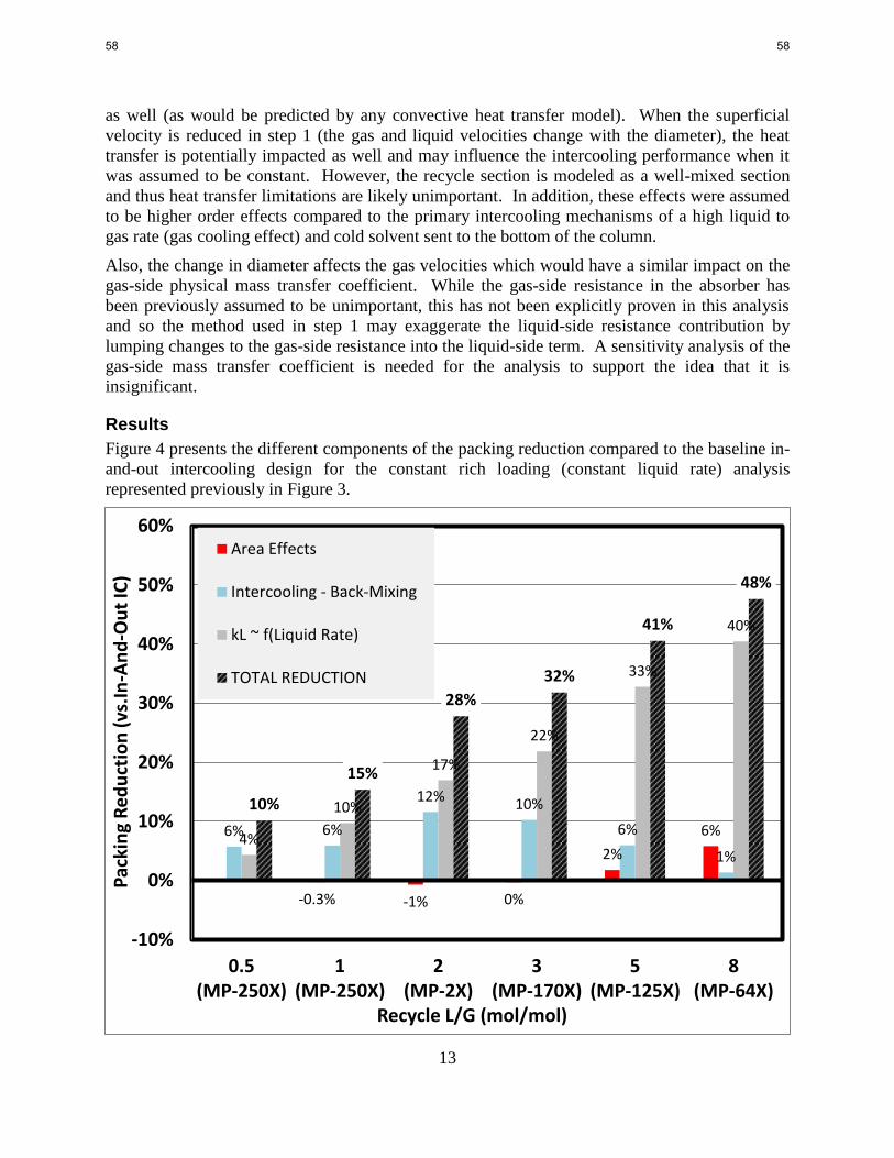
13

as well (as would be predicted by any convective heat transfer model). When the superficial

velocity is reduced in step 1 (the gas and liquid velocities change with the diameter), the heat

transfer is potentially impacted as well and may influence the intercooling performance when it

was assumed to be constant. However, the recycle section is modeled as a well-mixed section

and thus heat transfer limitations are likely unimportant. In addition, these effects were assumed

to be higher order effects compared to the primary intercooling mechanisms of a high liquid to

gas rate (gas cooling effect) and cold solvent sent to the bottom of the column.

Also, the change in diameter affects the gas velocities which would have a similar impact on the

gas-side physical mass transfer coefficient. While the gas-side resistance in the absorber has

been previously assumed to be unimportant, this has not been explicitly proven in this analysis

and so the method used in step 1 may exaggerate the liquid-side resistance contribution by

lumping changes to the gas-side resistance into the liquid-side term. A sensitivity analysis of the

gas-side mass transfer coefficient is needed for the analysis to support the idea that it is

insignificant.

Results

Figure 4 presents the different components of the packing reduction compared to the baseline in-

and-out intercooling design for the constant rich loading (constant liquid rate) analysis

represented previously in Figure 3.

-0.3% -1% 0%

2%

6% 6% 6%

12% 10%

6%

1% 4%

10%

17%

22%

33%

40%

10%

15%

28%

32%

41%

48%

-10%

0%

10%

20%

30%

40%

50%

60%

0.5(MP-250X)

1(MP-250X)

2(MP-2X)

3(MP-170X)

5(MP-125X)

8(MP-64X)

Pac

kin

g R

ed

uct

ion

(vs

.In

-An

d-O

ut

IC)

Recycle L/G (mol/mol)

Area Effects

Intercooling - Back-Mixing

kL ~ f(Liquid Rate)

TOTAL REDUCTION

58 58

14

Figure 4: Isolated contributions to overall packing reduction for recycle intercooling design

compared to in-and-out intercooling design. Recycle rates from 0.5 to 8 L/G are presented

for the natural gas combined cycle application. All cases with following specifications:

LLDG = 0.25 mols CO2/mols alkalinity, RLDG = 0.365 mols CO2/mols alkalinity, CO2

Removal = 90%.

The area effects (first bar in each group reading from left to right) include the combined effect of

liquid rate and packing specific area on the wetted area (or fractional area); the two were

combined since the overall contribution to the change in packing requirement is small in all

cases. The area effects are negative (or increase the packing requirement compared to in-and-out

intercooling) at the lowest recycle rates because the Hanley and Chen model predicts a negative

dependence on liquid velocity (as discussed before); as the packing is changed to progressively

coarser packing, however, the fractional area dependence on the packing geometry (negative

dependence on specific area of the packing) begins to become more important, and the area

effects ultimately contribute to a reduction in the packing requirement. In general, however, it is

clear that the Hanley and Chen model predicts minimal effect on wetted area of the packing

due to the conditions in the recycle.

The combined intercooling and back-mixing effect of the recycle (driving force effects) are

shown in the second bar from the left in each case. This trend shows an initially increasing

benefit from intercooling at the lowest recycle rates to a maximum of 12% packing reduction at

the 2 L/G recycle rate; beyond this recycle rate, the benefit diminishes and appears negligible at

the highest recycle rates. There are two explanations for this trend. First, as the recycle rate is

increased, the marginal benefit of intercooling diminishes – the temperature in the system is not

affected by an incremental increase in liquid rate beyond some point. This would explain a

flattening in intercooling benefits with recycle rate; the decline is explained by the back-mixing

contribution. As illustrated in Table 3, as the recycle rate increased, more of the packing was

allocated to the well-mixed recycle section of the column by the optimization. Therefore, the

average driving forces in the column are progressively diminished with recycle rates and

undercut the benefit from intercooling.

Finally, the last contribution to the overall packing reduction, is the effect of the liquid rate on

the mass transfer resistance (as determined indirectly from the modeling step (step 1) in the

procedure described before). The third bar from the left for each case reflects this contribution.

Clearly, this is the dominant source of the packing reduction predicted by the model. This result

indicates that the physical liquid-side mass transfer coefficient (as predicted by the Hanley and

Chen model) is of a magnitude where it is a significant contributor to the overall mass transfer

resistance; when coupled with the strong dependence on liquid rate predicted by the model, the

mass transfer resistance contribution becomes very important in the recycle configuration.

This highlights the importance of isolating these effects. If the intercooling benefit is the most

likely to be important in real systems or the model is most likely to accurately predict

intercooling benefits, the current design is less than optimal – the strong dependence on mass

transfer resistance contributions led to a large amount of packing in the middle of the column,

reducing average driving forces and wiping out the intercooling benefits. If the mass transfer

benefits are not realized at this magnitude in a real system, the design will lead to poor

performance compared to the cost of the recycle system (in particular, the pumping costs over

the large recycle section). Therefore, future work needs to determine which of the effects

59 59

15

isolated in this initial analysis are in fact significant and what a reasonable range of sensitivity is

for each parameter. This may come from literature review or evaluation of data collected in this

research group for specific conditions and types of packing.

Conclusions

A method was developed to isolate the different contributions to the packing reduction predicted

for the recycle intercooling configuration compared to the in-and-out configuration in an effort

provide a detailed understanding of the recycle design. The results of this evaluation are

summarized as follows:

The Hanley and Chen model predicts minimal contributions to packing reduction from

the effect of liquid rate and packing selection in the recycle section on the wetted area

available for mass transfer. The two effects (liquid rate and packing geometry)

effectively cancel over the range of conditions tested.

The driving force effects of the liquid recycle design (which includes an intercooling

benefit and penalty for back-mixing) initially show increasing benefits with recycle rate

(the marginal benefit of improved intercooling outweighs the back-mixing impact of the

recycle). The packing reduction from driving force effects reaches a maximum of 12% at

a recycle of 2L/G. At higher recycle rates (> 2L/G), the back-mixing effect becomes more important while

the incremental benefit of intercooling diminishes. This indicates that the current design

(increasing amount of packing in the recycle section with recycle rate) does not maximize

benefits from the intercooling effect. In addition, higher recycle rates may not provide

enough benefit from intercooling in general to justify increased pumping costs. The model predicts that the benefits of the recycle system are dominated by the

contribution of reduced liquid-side mass transfer resistance due to the increased liquid

rate in the recycle. The reduction packing from the mass transfer coefficient contribution

is as high as 40% (of the overall 48% reduction) for the highest recycle rate (8 L/G).

This effect drives the optimization to minimize total packing area by selectively putting

more packing in the middle (recycle) section of the column as the liquid rate is increased.

This strong dependence requires further investigation and should be subject to thorough

sensitivity analysis to determine if the benefits are realizable in a real system.

Process Safety Considerations

A critical component of large-scale deployment of amine based capture systems will be

management of solvent losses due to process failures or upsets. In the scope of the absorber, this

includes flooding of the absorber column which would lead to the potential venting of large

amounts of solvent. Several operating circumstances and components of absorber design should

be considered to prevent flooding of the column during operation:

1) Flooding Under Standard Operating Conditions: Flooding during normal operation is

primarily prevented during the equipment design process. Absorber designs typically

include a safety margin to prevent operation in the flooding region (70% to 80% of

flooding velocity). However, the flooding limit (and associated safety margin) is based on

pressure drop correlations specific to the packing type, operating conditions, and fluid

properties used in experimental development of the correlations. Therefore, an important

aspect of absorber design for novel solvents and configurations (e.g., recycle

60 60

16

intercooling) is testing and development of correlations relevant to amine scrubbing for

power plant applications. This includes experimental efforts such as air-water packing

experiments and pilot scale operations such as those conducted within our group at the

Pickle Research Center.

2) Flooding Due to Equipment Failure: This category includes scenarios such as the failure

of equipment downstream of the absorber. For example, shutdown or failure of pumps

downstream of the absorber could lead to accumulation of liquid in the absorber and and

eventually flooding of the column. Prevention measures would include level sensors in

the absorber sump to trigger shutdown of feed flows, pump sparing or pumping to

emergency solvent storage, and shutdown associated with pressure drop measurements in

the absorber.

3) Flooding during start-up/shut-down: This scenario is particularly relevant to capture

applications for power plants where flexible operation of the scrubbing system or power

plant conditions may require frequent cycling of the amine scrubbing system. During

ramping/shutdown of the capture system, gas and liquid flow rates to the absorber must

be carefully controlled in tandem; high gas velocities (relative to the liquid rate) can be

realized in the absorber that would not be observed in normal operations. Pressure drop

sensors, liquid level control sensors, and flow meters for the gas and liquid can be used to

provide data to design a control strategy to avoid flooding conditions during ramping.

Future Work

The intercooling evaluation performed for coal and natural gas applications will be considered in

further detail using the new information from the isolation of benefits. The mass transfer model

dependencies on packing selection and liquid rate will be evaluated from a range of literature

models and experimental data in our group to provide means for a sensitivity analysis. Alternate

methods to isolate benefits of the recycle design will be considered. For example, the prediction

of a minimum liquid rate for different configurations (or different recycle rates) can serve as a

proxy for the intercooling benefits realized by a design (equilibrium pinches removed). The

findings will be extended to selection of packing to optimize performance in the recycle section

and development of new absorber configuration concepts.

References

Hanley B, Chen CC. “New Mass-Transfer Correlations for Packed Towers.” AICHE J.

2012;58:132–152.

Henriques de Brito M, von Stockar U, Menendez Bangerter A, Bomio P, Laso M. “Effective

Mass-Transfer Area in a Pilot Plant Column Equipped with Structured Packings and with

Ceramic Rings.” Ind Eng Chem Res. 1994;33:647–656.


Piperazine, and Promoted Potassium Carbonate. The University of Texas at Austin. Ph.D.

Dissertation. 2011.

Rochelle GT et al. "CO2 Capture by Aqueous Absorption, Fourth Quarterly Progress Report


Tsai RE. Mass Transfer Area of Structured Packing. The University of Texas at Austin. Ph.D.

Dissertation. 2010.

61 61

1

Modeling and Optimization of

Advanced Stripper Configurations


by Yu-Jeng Lin




July 31, 2013

Abstract

In this work, advanced stripper configurations have been modeled and optimized using Aspen

Plus®. Equivalent work is used as an indicator of energy performance as well as heat duty. A

rich exchanger bypass strategy that recovers stripping steam heat by using a cross exchanger has

been proposed. To get better energy performance, this strategy is applied to advanced stripper

configurations. The next pilot plant configuration, flash stripper with warm rich bypass and rich

exchanger bypass, has offered an 8.4% energy improvement for 8 m PZ and 4.4% for 9 m MEA.

One objective of this work is to demonstrate the flexibility with different operating temperature

of the flash stripper with warm rich bypass and rich exchanger bypass. Since existing power

plants may have different pressure levels of steam extracted from the crossover pipe between the

low and intermediate pressure turbines, the stripper needs to adapt to different operating

temperatures. By equivalent work analysis, the flexibility of this configuration has been

demonstrated in the operating range from 120–150 oC for 8 m PZ and 120–135

oC for 9 m MEA.

When comparing two different regeneration temperatures, the higher operating temperature has

greater improvement at lower lean loading but is less efficient at higher loading.

Another objective is to investigate energy performance using 5 m PZ. 5 m PZ has lower

viscosity, which leads to a higher heat transfer coefficient. Even though 5 m PZ has lower CO2

capacity which increases the sensible heat, but less heat exchanger area is required to attain the

same temperature approach. A preliminary comparison of 5 m and 8 m PZ has been done using

the same 5 oC LMTD specifications in the cross exchanger.

Introduction

In post-combustion CO2 capture, steam usage for lean solvent regeneration in the stripper and

CO2 compression work are the main contributions to the energy requirement. Implementing CO2

capture incurs a 20–30% penalty on electricity output for a typical coal-fired power plant

(Rochelle, 2009). Alternative stripper configurations could improve energy efficiency

significantly compared to a simple stripper.

62 62

2

Several previous studies have been done to improve equivalent work by introducing alternative

stripper configurations. Oyenekan (2007) proposed matrix, internal exchange, multi-pressure,

and flashing feed stripper configurations. The best performance case was obtained in a matrix

with MDEA/PZ, improving energy savings by 22% over the simple stripper. Van Wagener

(2011) emphasized the importance of increasing process reversibility by introducing more

complex configurations including multi-stage flash, cold rich bypass, and an interheated column.

Van Wagener showed that the interheated column with 8 m PZ offers the best energy savings.

To improve capture efficiency, stripper modeling and optimization of novel configurations have

been done using Aspen Plus® software.

Loss of steam heat from the stripper is one of the reasons that CO2 capture by amine scrubbing is

inefficient. When the stripper is operated at 120–150 oC, water in the rich solvent is vaporized

and emitted with CO2 from the top of stripper. Flashing can be reduced using cold rich bypass.

Another possible method is the rich exchanger bypass applying a heat exchanger to recover

steam heat by bypassing cold rich solvent. Several advanced stripper configurations modified by

rich exchanger bypass have been proposed. A flash stripper with warm rich bypass and rich

exchanger bypass that offers 9% energy improvement for PZ and 6% for MEA will be used for

the next pilot plant campaign.

This work demonstrates the flexibility to use variable operating temperature with the flash

stripper with warm rich bypass and rich exchanger bypass. Since the existing power plants may

have different steam pressure at the crossover pipe between the low and intermediate pressure

turbine, the stripper needs flexibility to adapt to different operating temperature.

This work also investigates energy performance using 5 m PZ. The motivation for using 5 m PZ

is its lower viscosity leading to a higher heat transfer coefficient. Compared to 8 m PZ, 5 m PZ

has lower CO2 capacity which increases the sensible heat required but less heat exchanger area is

required to attain same temperature approach because of higher heat transfer coefficient. The

trade-offs between different concentrations of PZ are the capital cost of the heat exchanger and

sensible heat required.

Methods

A simple stripper with 2 meter packing was chosen as the base case. The following cases were

studied:

1. Simple stripper using 8 m PZ and 9 m MEA.

2. Flash stripper with warm rich bypass and rich exchanger bypass using 8 m PZ with 150 oC

steam heater temperature.



4. Flash stripper with warm rich bypass and rich exchanger bypass using 9 m MEA with 135 oC


5. Flash stripper with warm rich bypass and rich exchanger bypass using 9 m MEA with 120 oC




63 63

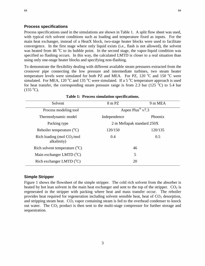
3

Process specifications

Process specifications used in the simulations are shown in Table 1. A split flow sheet was used,

with typical rich solvent conditions such as loading and temperature fixed as inputs. For the

main heat exchanger, instead of a HeatX block, two-stage heater blocks were used to facilitate

convergence. In the first stage where only liquid exists (i.e., flash is not allowed), the solvent

was heated from 46 oC to its bubble point. In the second stage, the vapor-liquid condition was

specified so flashing occurs. In this way, the calculated LMTD is closer to a real situation than

using only one-stage heater blocks and specifying non-flashing.

To demonstrate the flexibility dealing with different available steam pressures extracted from the

crossover pipe connecting the low pressure and intermediate turbines, two steam heater

temperature levels were simulated for both PZ and MEA. For PZ, 120 oC and 150

oC were

simulated. For MEA, 120 oC and 135

oC were simulated. If a 5

oC temperature approach is used

for heat transfer, the corresponding steam pressure range is from 2.3 bar (125 oC) to 5.4 bar

(155 oC).

Table 1: Process simulation specifications.

Solvent 8 m PZ 9 m MEA

Process modeling tool Aspen Plus® v7.3

Thermodynamic model Independence Phoenix

Packing type 2 m Mellapak standard 250X

Reboiler temperature (oC) 120/150 120/135

Rich loading (mol CO2/mol

alkalinity)

0.4 0.5

Rich solvent temperature (oC) 46

Main exchanger LMTD (oC) 5

Rich exchanger LMTD (oC) 20

Simple Stripper

Figure 1 shows the flowsheet of the simple stripper. The cold rich solvent from the absorber is

heated by hot lean solvent in the main heat exchanger and sent to the top of the stripper. CO2 is

regenerated in the stripper with packing where heat and mass transfer occur. The reboiler

provides heat required for regeneration including solvent sensible heat, heat of CO2 desorption,

and stripping steam heat. CO2 vapor containing steam is fed to the overhead condenser to knock

out water. The CO2 product is then sent to the multi-stage compressor for further storage and

sequestration.

64 64

4

CO2 product

Main

Exchanger

Hot Lean Solvent

Reboiler

Stripper

Knocked out

water

Rich solvent

46 oC

0.40 Ldg. (PZ)

0.50 Ldg. (MEA)

Figure 1: Simple stripper.

Flash Stripper with Warm Rich Bypass and Rich Exchanger Bypass

Figure 2 shows the flash stripper with warm rich bypass and rich exchanger bypass. In this

configuration, a cross exchanger is used to preheat cold rich solvent by hot CO2 vapor coming

out of the stripper. A portion of the cold rich solvent obtains latent heat of steam from the

stripped vapor. Warm rich bypass is extracted between two cross exchangers and fed to the top

of the stripper after mixing with cold rich bypass. The temperature was selected as the bubble

point temperature at the stripper operating pressure. The rest of the rich solvent is heated by a

steam heater and fed into the bottom of the flash stripper. The reboiler found in a typical stripper

is replaced by a steam heater and a flash vessel. Only part of the rich solvent countercurrently

contacts with vapor in the flash stripper.

To reduce the inefficiency caused by stripping steam heat, either cold rich bypass or rich

exchanger bypass can be used. For both strategies, stripping steam heat can be recovered either

in the cross exchanger or in the stripper, which serves as a direct contact cooler. In Q1 2013, it

was demonstrated that using a cross exchanger is more efficient. In this configuration (Figure 2),

both concepts are applied. Warm rich bypass condenses part of the stripping steam in the

stripper and the cold rich bypass recovers the rest. Applying warm rich bypass makes the heat

transfer driving force between rich solvent and hot CO2 vapor smaller in both the stripper and the

rich exchanger. It works more reversibly and efficiently than rich exchanger bypass and cold

rich bypass.

Since it has less solvent hold-up and residence time the steam heater will minimize thermal

degradation. The capital cost of a convective steam heater should be less than than a reboiler.

65 65

5

Main

Exchanger

Hot Lean

CO2 Vapor

Rich

ExchangerCO2 to

Compression

Warm Rich Bypass

Rich solvent

46 oC

0.40 Ldg. (PZ)

0.50 Ldg. (MEA)

Cold Rich Bypass

Lean solvent

Steam Heater

Flash

Stripper

Figure 2: Flash stripper with warm rich bypass and rich exchanger bypass.

Equivalent Work Calculation

Equivalent work is more useful metric of energy use than heat duty alone. As Equation 1 shows,

equivalent work consists of pump work, compression work, and heat work. The pump is

required to move the solvent from the absorber to the pressure and height of the stripper. Heat

work is obtained from heat duty by Equation 2. The turbine efficiency, is set to a typical value

of 75%.

(

)

(

)

Compression work is calculated by Equation 3 as a function of suction pressure to a discharge

pressure of 150 bar.

(

)

{

(

)

(

)


Variable regeneration temperature

Figures 3 and 4 show the flash stripper with warm rich bypass and rich exchanger bypass

operated at different temperature using 8 m PZ and 9 m MEA, respectively. Optimum

equivalent work can be obtained by varying lean loading. Higher lean loading leads to higher

66 66

6

CO2 partial pressure. When lean loading increases, the stripping steam heat required and

compression work decreases, but sensible heat increases because of reduced capacity.

Comparing a simple stripper and flash stripper at the same operating temperature, the

improvement comes from the recovery of stripping steam heat. At lower lean loading, the flash

stripper shows greater improvement because more stripping steam is available to be recovered.

To demonstrate flexibility dealing with different operating temperature, the lower temperature

case (120 oC) was simulated for 8 m PZ and the higher temperature case (135

oC) for 9 m MEA.

With lower temperature, the ratio of stripping steam to CO2 removed becomes higher. Stripping

steam heat required is the main factor causing the inefficiency of the lower temperature case at

lower lean loading. However, as lean loading increases, the equivalent work of the two

temperature cases get closer and the crossover is near 0.34 lean loading for PZ and 0.42 for

MEA. The reason that the higher temperature case becomes inefficient at higher lean loading is

that the heat duty at higher temperature is more valuable (from Carnot cycle efficiency

expression). At higher lean loading, the difference in stripping steam heat required between two

temperature cases is not that significant so that the Carnot cycle efficiency term becomes a more

important factor.

In a higher temperature case, the shift of optimum lean loading toward a lower value can be

observed because when temperature increases, the contribution of stripping steam heat to total

equivalent work becomes less compared to the contribution of sensible heat.

Table 2: Optimum process conditions for flash stripper with warm bypass and rich

exchanger bypass operated at different temperatures.

Solvent T (oC)

Lean Ldg.

(mol CO2/mol Alk.)

Cold Bypass(%)/

Warm Bypass Rate

(%)

Pressure

(bar)

Qreb

(kJ/mol

CO2)

Weq

(kJ/mol

CO2)

8 m PZ 150 0.30 5/10 8.2 91.5 29.0

120 0.32 6/12 3.0 102.9 30.6

9 m

MEA

135 0.36 7/10 5.3 122.2 34.2

120 0.38 9/14 2.9 132.0 35.5

67 67

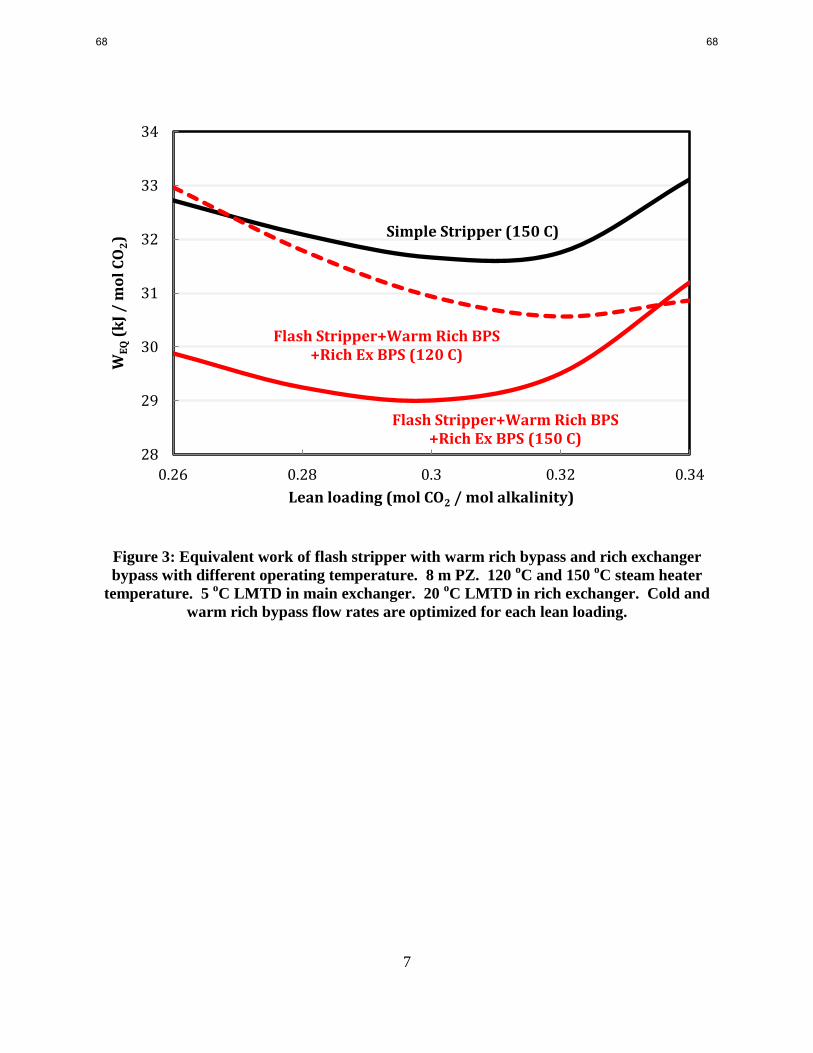
7

Figure 3: Equivalent work of flash stripper with warm rich bypass and rich exchanger

bypass with different operating temperature. 8 m PZ. 120 oC and 150

oC steam heater

temperature. 5 oC LMTD in main exchanger. 20

oC LMTD in rich exchanger. Cold and

warm rich bypass flow rates are optimized for each lean loading.

28

29

30

31

32

33

34

0.26 0.28 0.3 0.32 0.34

WE

Q (

kJ

/ m

ol

CO

2)

Lean loading (mol CO2 / mol alkalinity)

Simple Stripper (150 C)

Flash Stripper+Warm Rich BPS +Rich Ex BPS (150 C)

Flash Stripper+Warm Rich BPS +Rich Ex BPS (120 C)

68 68

8


bypass with different operating temperature. 9 m MEA. 120 oC and 135

oC steam heater

temperature. 5 oC LMTD in main exchanger. 20

oC LMTD in rich exchanger. Cold and

warm rich bypass flowrates are optimized for each lean loading.

Energy performance of 5 m and 8 m PZ

The comparison of 5 m and 8 m PZ requires a tradeoff of cross-exchanger capital cost and heat

duty for sensible heat. Two possible approaches could be used to quantify the potential benefit

of a lower concentration of PZ (5 m). One is fixing the LMTD of the cross exchanger in both

cases. Less exchanger area is required for 5 mPZ due to lower viscosity. Economic analysis

could be done by pricing the exchanger area and energy requirement. The other way is to get

LMTD from the given heat transfer coefficient correlation and viscosity. A lower concentration

of PZ can be expected to have a smaller LMTD. Then different amine concentration cases can

be compared directly by total equivalent work.

Figure 5 shows the equivalent work of the flash stripper with warm rich bypass and rich

exchanger bypass using 5 m PZ and 8 m PZ. The simulations for each case were done by fixing

LMTD of the cross exchanger at 5 oC. Comparing the equivalent work between 5 m and 8 m,

the difference is more significant at higher lean loading. For PZ, CO2 partial pressure is not a

function of amine concentration at a given loading and temperature (Dugas, 2009), so the only

factor resulting in the difference is the sensible heat. Also, the optimum lean loading for 5 m PZ

is shifted toward lower value because the contribution of sensible heat to total equivalent work

becomes greater.

34

35

36

37

38

39

0.3 0.32 0.34 0.36 0.38 0.4 0.42 0.44

WE

Q (

kJ

/ m

ol

CO

2)


Simple Stripper (120 C)

Flash Stripper+Warm Rich BPS + Rich Ex BPS (120 C)

Flash Stripper +Warm Rich BPS + Rich Ex BPS (135 C)

69 69

9


bypass with different operating temperature. 150 oC steam heater temperature. 5

oC

LMTD in main exchanger. 20 oC LMTD in rich exchanger. Cold and warm rich bypass

flowrates are optimized for each lean loading.

Conclusions

1. The flexibility of the flash stripper with warm rich bypass and rich exchanger bypass

configuration has been demonstrated in the operating range from 120–150 oC for 8 m PZ and

120–135 oC for 9 m MEA.

2. When comparing two different temperature level cases, the higher operating temperature case

shows greater improvement at lower lean loading but is less efficient at higher loading due to the

Carnot cycle efficiency term from heat-work conversion.

3. With the flash stripper using a warm rich bypass and rich exchanger bypass, 9 m MEA uses

1.5 to 3 kJ/mol less work with stripping at 135 oC rather than 120

oC. The convective steam

heater should make higher temperature feasible with acceptable thermal degradation.

4. With the flash stripper using a warm rich bypass and rich exchanger bypass, 5 m PZ gives the

same performance as 8 m PZ at a lean loading of 0.26 (assuming a an exchanger LMTD of 5 oC.

5. Preliminary comparison of 5 m and 8 m PZ has been done using the same 5 oC LMTD

specifications in the cross exchanger.

28

29

30

31

32

33

34

35

36

37

0.22 0.24 0.26 0.28 0.3 0.32 0.34

WE

Q (

kJ

/ m

ol

CO

2)


Simple Stripper (8m PZ)

Flash Stripper +Warm Rich BPS+Rich Ex BPS (8m PZ)

Flash Stripper+Warm Rich BPS +Rich Ex BPS (5m PZ)

Simple Stripper (5m PZ)

70 70

10

Future Work

1. Lost work analysis of stripper configurations will be investigated to see where the inefficiency

is and if it has room to improve.

2. To quantify 5 m PZ energy performance, LMTD can be found by given heat transfer

coefficient correlation and viscosity. Total equivalent work will be used as an indicator to

compare 5 m and 8 m PZ.

3. New alternative stripper configurations.

References

Dugas RE. Carbon Dioxide Absorption, Desorption, and Diffusion in Aqueous Piperazine and

Monoethanolamine. The University of Texas at Austin. Ph.D. Dissertation. 2011.

Oyenekan B. Modeling of Strippers for CO2 Capture by Aqueous Amines. The University of

Texas at Austin. Ph.D. Dissertation. 2007.

Rochelle GT. "Amine scrubbing for CO2 capture". Science. 2009;325,1652–24.

Van Wagener DH. Stripper Modeling for CO2 Removal Using Monoethanolamine and

Piperazine Solvents. The University of Texas at Austin. Ph.D. Dissertation. 2011.

71 71

1

2MPZ Kinetic Model and 2MPZ/PZ Model


by Brent Sherman


and the Carbon Capture Simulation Initiative



July 31, 2013

Abstract

The kinetic model of 8 m 2-methylpiperazine (2MPZ) now matches the majority of the

experimental fluxes within 20%. There is a systematic bias with temperature, but no bias is

apparent with loading. Comparison of the reaction pre-exponentials for 8 m 2MZP to 8 m PZ

shows that the steric hindrance of the α-methyl group lowers the pre-exponential of the

carbamate and dicarbamate by 30% and 54% respectively (1.45E10 compared to 2.04E10 and

1.28E10 compared to 2.76E10 kmol/s-m3). The increased viscosity of 2MPZ leads to diffusion

of amine and products being approximately 10% slower than in the PZ system. A procedure for

merging two existing thermodynamic models was developed and implemented by blending

2MPZ into the Independence model.

Introduction

This work has four goals: rigorous thermodynamic and kinetic models, a generic amine modeling

method, economic evaluation, and viscosity process effects. Developing more rigorous models

offers the necessary insight into model development to create a generic amine modeling method.

The aim of the method is to streamline model development, thus allowing more rapid screening

of solvents. Then, using the rigorous and generic models, process performance can be evaluated

from an economic standpoint with special interest paid to viscosity effects. For more detail, see

the research proposal in Appendix A.

Work this quarter focused on the 8 m 2-methylpiperazine (2MPZ) kinetic model as well as

merging the 2MPZ thermodynamic model into the existing MDEA/PZ Independence model.

The procedure for these has been documented in Appendix B. Appendix C contains two posters

that were presented at the April Industry Advisory Board meeting for the Carbon Capture

Simulation Initiative (CCSI). Additional work this quarter involved coordinating with CCSI and

supporting uncertainty quantification of the Phoenix MEA model (Plaza, 2011).

Safety: Pressure Relief

While the absorber operates at atmospheric pressure, the stripper or flash vessel can operate at

higher than 10 bar. This requires the lean pump to take that pressure also. Whenever there is

even the potential for greater than atmospheric pressure, a pressure relief valve must be used.

72 72

2

The pilot plant at the Pickle Research Campus uses two different valve types: conventional

spring and balanced bellows, as shown in Figure 1. The conventional spring type is used on the

stripper and flash vessels, and the balanced bellows is used on the lean amine pump. The

bellows design protects the delicate moving parts from corrosive amine solution, while the

conventional spring is sufficient for the stripper and flash vessels as it will relieve only gases.

Figure 1: Two different pressure relief valves. The bellows design protects the relief spring

from corrosion.

Modeling Methods

8 m 2MPZ Kinetic Modeling

The procedure used last quarter was significantly modified (Rochelle et al., 2013a). The reaction

set, shown in Table 1, and ratio (kcarbamate = 0.88kdicarbamate) between the carbamate and

dicarbamate remained the same. The methods for loading adjustment and calculation of rate

constants ko and activation energies EA were changed. The diffusivity parameters of Equation 1

were also regressed.

0465.0ref

oT

TDD (1)

In order to calculate ko and EA, two points were chosen at different loadings: one where the

bicarbonate reaction is insignificant, and a higher one where the bicarbonate is significant. At

each of these points, the 40 °C and 60 °C fluxes were examined. Using a fixed set of kinetic

parameters—in contrast to last quarter where the reaction parameters were varied—the

simulation was run with the goal of matching the over- or underpredictions of the fluxes. This

ensures that the line fit to the experimental data passes through the origin, meaning that at zero

driving force, there is zero flux. This adjustment was done until the ratio of predicted flux to

actual flux for the absorption and desorption points were within 1% of each other, or until the

loading had been adjusted up to 10% of the operational loading range. Thus, the maximum

loading adjustment was ±0.01 mol CO2/mol alk.

Once this loading adjustment was completed, a design specification was used to match the flux

exactly by varying the ko of one reaction. During this regression, the EA was set to zero. Thus,

73 73

3

ko is equal to k, allowing the calculation of EA. (Recall the power law kinetic form from Rochelle

et al. (2013a)). This was done for both temperatures, and then EA was calculated.

ko and EA were fixed, and the same procedure for loading adjustment used previously was

applied to every data point. The diffusivity parameters were changed, and the loading

adjustment was again applied to every data point. This process was repeated as necessary. A

more detailed procedure is included in Appendix C.

Merging Models

As a first step towards a model of 4 m PZ/4 m 2MPZ, the thermodynamic 2MPZ model was

incorporated into the Independence model. In order to ensure that the 2MPZ in the incorporated

model is the same as the 2MPZ in the source model, thermodynamic verification was repeated.

A procedure for such merges was developed and is included in Appendix C.


8 m 2MPZ Kinetic Modeling

Using a very small reaction set, most of the data were matched within 20%. There were 9

predicted fluxes not within 20% of the experimental fluxes. The kinetic fit is displayed in

Figures 2 and 3. As seen in Figure 2, the predictions worsen at higher temperatures as

experimental error increases. In addition to the random dispersion trend with increasing

temperature, there is a linear systematic bias. Efforts to correct for this bias by changing the

reference temperature for diffusivity were unsuccessful. Figure 3 shows no systematic trend

with loading, and the dispersion with temperature remains approximately constant.

The kinetic fit for 8 m PZ is shown in Figures 4 and 5. Figure 4 shows that there is no

systematic bias with temperature. However, all fluxes are underpredicted at 80 °C. Figure 5

shows no systematic bias with loading. However, all data are overpredicted at 0.34 loading and

underpredicted at 0.289 and 0.412 loading. Nevertheless, all of these predicted fluxes are very

close to the experimental values. Comparing Table 1 and Table 2 demonstrates the steric

hindrance effect of the α-methyl group of 2MPZ. Dividing the ko values of 2MPZ by those of

PZ for carbamate, dicarbamate, and bicarbonate reactions yields 0.71, 0.46, and 120,

respectively. The hindrance leads to slower rates for the carbamate and dicarbamate reactions,

which is intuitive. The bicarbonate reaction is expedited owing to the increased instability of the

carbamate relative to the bicarbonate. This is reflected in the increased concentration of

bicarbonate at equilibrium as shown in Figure 6 of Rochelle et al. (2013b).

Looking at the diffusivities of 2MPZ and PZ in Table 3 shows that 2MPZ is only slightly slower

than PZ. Table 4 shows that the dependence of diffusivity on viscosity is equal for both.

However, 2MPZ has a viscosity that is double that of PZ (~20 cP vs ~10 cP depending on

temperature and loading). Thus, the same exponential will carry greater weight with 2MPZ than

with PZ. This is countered by the normalizing viscosity for PZ being 0.0155 cP. As for the

temperature dependence, the exponent for 2MPZ is far greater than that for PZ. This is probably

indicative not of a physical effect, but of the diffusivity being distorted to fit temperature

dependence effects.

74 74

4

Table 1: Reaction set for 2MPZ. Dicarbamate 2 orders slower than for PZ.

Reaction ko (kmol/s-m3) EA (kJ/mol)

2MPZCOO- + H2O + CO2 H2MPZCOO + HCO3-

2.62E6 98.0

2 2MPZ + CO2 2MPZH+ + 2MPZCOO- 1.45E10 21.9

2 2MPZCOO- + CO2 2MPZ(COO-)2 + H2MPZCOO 1.28E10 21.9

H2MPZCOO + HCO3- 2MPZCOO- + H2O + CO2

3.67E5 174

2MPZH+ + 2MPZCOO 2 2MPZ + CO2 3.96E4 97.8

2MPZ(COO-)2 + H2MPZCOO 2 2MPZCOO- + CO2 2.71E8 129

Table 2: PZ/MDEA Independence kinetic model parameters (Frailie et al., 2013).

Reaction ko (kmol/s-m3) EA (kJ/mol)

MDEA + H2O + CO2 MDEAH+ + HCO3- 5.17E3 44.9

PZCOO- + H2O + CO2 HPZCOO + HCO3- 2.19E4 49.0

2 PZ + CO2 PZH+ + PZCOO- 2.04E10 14.24 PZ + MDEA + CO2 PZCOO- + MDEAH+ 3.56E10 20.47 2 PZCOO- + CO2 PZ(COO-)2 + HPZCOO 2.76E10 14.24 PZCOO- + MDEA + CO2 PZCOO-

2 + MDEAH+ 4.83E10 20.47

MDEAH+ + HCO3- MDEA + CO2 + H2O 39.03 85.9

HPZCOO + HCO3- PZCOO- + H2O + CO2 64.64 92.1

PZH+ + PZCOO- 2 PZ + CO2 4.27E4 85.1 PZCOO- + MDEAH+ PZ + MDEA + CO2 9.25E5 85.6 PZ(COO-)2 + HPZCOO 2 PZCOO- + CO2 2.63E5 89.3 PZ(COO-)2 + MDEAH+ PZCOO- + MDEA + CO2 3.77E6 108.3

Table 3: Diffusivities of 8 m 2MPZ and 8 m PZ at lean loading. 2MPZ values are this

work, Independence values (Frailie et al., 2013).

T (K) D2MPZ (sqm/sec) DPZ (sqm/sec)

313.15 1.32E-09 1.48E-09 333.15 1.97E-09 2.13E-09 373.15 3.69E-09 3.88E-09

Table 4: Diffusivity parameters. 2MPZ values are this work, Independence values (Frailie

et al., 2013).

Diffusivity Parameter 8 m 2MPZ value

8 m PZ value

Do 4.4E-11 m2/s 1.42E-10 m2/s

α -1.50 -1.50

β -11.5 -2.58

Tref 373.15 K 373.15 K

75 75

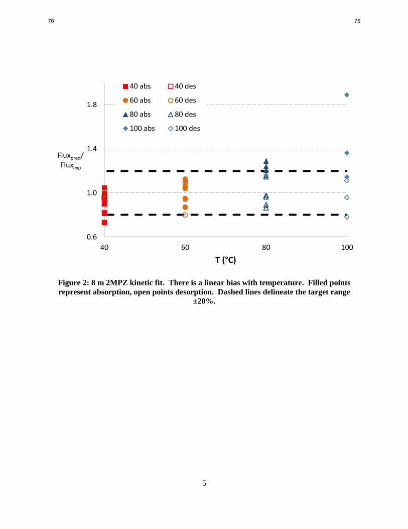
5

Figure 2: 8 m 2MPZ kinetic fit. There is a linear bias with temperature. Filled points

represent absorption, open points desorption. Dashed lines delineate the target range

±20%.

0.6

1.0

1.4

1.8

40 60 80 100

Fluxpred/ Fluxexp

T (°C)

40 abs 40 des

60 abs 60 des

80 abs 80 des

100 abs 100 des

76 76

6

Figure 3: 8 m 2MPZ kinetic fit. Model flux ratioed to experimental flux shows no clear

trend with loading. Filled points represent absorption, open points desorption. The

dashed lines delineate the target range ±20%.

Figure 4: 8 m PZ kinetic fit from Independence. There is no overall trend with loading, but

all data are underpredicted at 80 °C. From Frailie et al., 2013.

0.102 0.102 0.102 0.102 0.154 0.154 0.154 0.154 0.203 0.203 0.203 0.203 0.253 0.253 0.253 0.3 0.3 0.3 0.365 0.365

0.6

1.0

1.4

1.8

Fluxpred/ Fluxexp

Loading (mol/mol alk.)

40 abs 40 des

60 abs 60 des

80 abs 80 des

100 abs 100 des

0.88

0.92

0.96

1.00

1.04

1.08

40 60 80 100

Fluxpred/ Fluxexp

T (°C)

40 abs 40 des

60 abs 60 des

80 abs 80 des

100 abs 100 des

77 77

7

Figure 5: 8 m PZ kinetic fit. There is no overall trend, however all data are overpredicted

at 0.34 loading and underpredicted at 0.289 and 0.412 loading. From Frailie et al., 2013.

4 m PZ/4 m 2MPZ Model

Following the procedure given in methods and detailed in Appendix B, the 2MPZ

thermodynamic model was incorporated into Independence. After the merge, the thermodynamic

model for 2MPZ was re-validated to ensure all parameters had been transferred. The results are

identical to those shown in the first quarterly progress report for this year (Rochelle et al.,

2013b), and so will not be reproduced here. This completes the first and second steps in

sequential regression for a PZ/2MPZ model, namely amine–water and amine–water–carbon

dioxide.

Conclusions

1. The steric hindrance of 2MPZ results in a 30% lower carbamate reaction pre-exponential

and a 54% lower dicarbamate reaction pre-exponential relative to PZ

2. There is a systematic linear bias with temperature in the kinetic 2MPZ model (

); there is no bias with loading.

3. 31 out of 41 8 m 2MPZ experimental fluxes are matched within 20%.

4. The 2MPZ in the 2MPZ/PZ thermodynamic model is identical to the 2MPZ in the pure

2MPZ model, indicating a successful merge.

Future Work

The kinetic fit of 8 m 2MPZ will continue to be improved by adjusting reaction rates and

diffusion parameters. With a 2MPZ model in the blend model, regression of thermodynamic 4 m

2MPZ/4 m PZ data will begin. This will immediately involve regression of NRTL parameters

0.235 0.253 0.289 0.311 0.34 0.412

0.88

0.92

0.96

1.00

1.04

1.08

Fluxpred/ Fluxexp


40 abs 40 des

60 abs 60 des

80 abs 80 des

100 abs 100 des

78 78

8

for the ternary system of PZ–2MPZ–water, and then regression of e-NRTL parameters for the

quaternary system PZ–2MPZ–water–carbon dioxide.

References

Frailie PT, Madan T, Sherman B, Rochelle GT. “Energy Performance of Advanced Stripper

Configurations.” GHGT-11, Kyoto 2012.


Piperazine and Promoted Potassium Carbonate. The University of Texas at Austin, Ph. D.

Dissertation. 2011.

Rochelle GT et al. "CO2 Capture by Aqueous Absorption, First Quarterly Progress Report 2013."

Texas Carbon Management Program. The University of Texas at Austin. 2013a.


2012." Luminant Carbon Management Program. The University of Texas at Austin. 2013b.

Appendix A: Research Proposal

79 79

9



PhD Dissertation Proposal

Generic Amine Solvent Modeling

for CO2 Capture

Brent Sherman

Supervisor: Dr. Gary Rochelle

May 2013

80 80

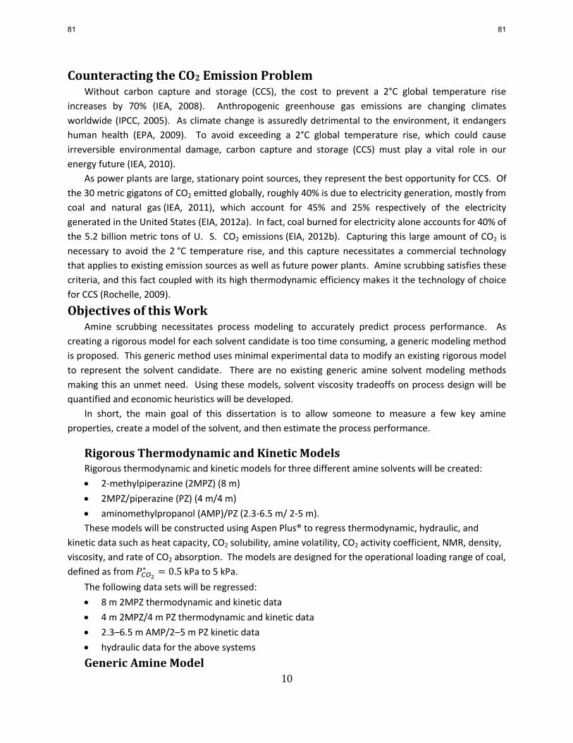
10

Counteracting the CO2 Emission Problem Without carbon capture and storage (CCS), the cost to prevent a 2°C global temperature rise

increases by 70% (IEA, 2008). Anthropogenic greenhouse gas emissions are changing climates

worldwide (IPCC, 2005). As climate change is assuredly detrimental to the environment, it endangers

human health (EPA, 2009). To avoid exceeding a 2°C global temperature rise, which could cause

irreversible environmental damage, carbon capture and storage (CCS) must play a vital role in our

energy future (IEA, 2010).

As power plants are large, stationary point sources, they represent the best opportunity for CCS. Of

the 30 metric gigatons of CO2 emitted globally, roughly 40% is due to electricity generation, mostly from

coal and natural gas (IEA, 2011), which account for 45% and 25% respectively of the electricity

generated in the United States (EIA, 2012a). In fact, coal burned for electricity alone accounts for 40% of

the 5.2 billion metric tons of U. S. CO2 emissions (EIA, 2012b). Capturing this large amount of CO2 is

necessary to avoid the 2 °C temperature rise, and this capture necessitates a commercial technology

that applies to existing emission sources as well as future power plants. Amine scrubbing satisfies these

criteria, and this fact coupled with its high thermodynamic efficiency makes it the technology of choice

for CCS (Rochelle, 2009).

Objectives of this Work Amine scrubbing necessitates process modeling to accurately predict process performance. As

creating a rigorous model for each solvent candidate is too time consuming, a generic modeling method

is proposed. This generic method uses minimal experimental data to modify an existing rigorous model

to represent the solvent candidate. There are no existing generic amine solvent modeling methods

making this an unmet need. Using these models, solvent viscosity tradeoffs on process design will be

quantified and economic heuristics will be developed.

In short, the main goal of this dissertation is to allow someone to measure a few key amine

properties, create a model of the solvent, and then estimate the process performance.

Rigorous Thermodynamic and Kinetic Models Rigorous thermodynamic and kinetic models for three different amine solvents will be created:

2-methylpiperazine (2MPZ) (8 m)

2MPZ/piperazine (PZ) (4 m/4 m)

aminomethylpropanol (AMP)/PZ (2.3-6.5 m/ 2-5 m).

These models will be constructed using Aspen Plus® to regress thermodynamic, hydraulic, and

kinetic data such as heat capacity, CO2 solubility, amine volatility, CO2 activity coefficient, NMR, density,

viscosity, and rate of CO2 absorption. The models are designed for the operational loading range of coal,

defined as from kPa to 5 kPa.

The following data sets will be regressed:

8 m 2MPZ thermodynamic and kinetic data

4 m 2MPZ/4 m PZ thermodynamic and kinetic data

2.3‒6.5 m AMP/2‒5 m PZ kinetic data

hydraulic data for the above systems

Generic Amine Model

81 81

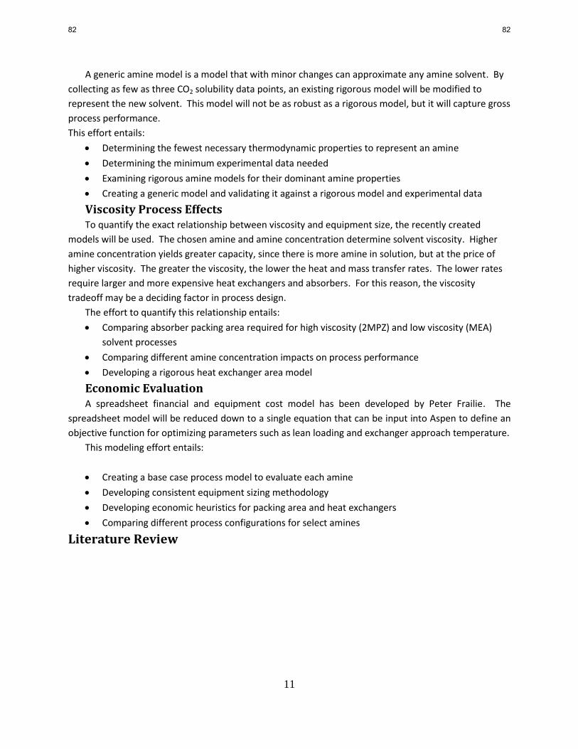
11

A generic amine model is a model that with minor changes can approximate any amine solvent. By

collecting as few as three CO2 solubility data points, an existing rigorous model will be modified to

represent the new solvent. This model will not be as robust as a rigorous model, but it will capture gross

process performance.

This effort entails:

Determining the fewest necessary thermodynamic properties to represent an amine

Determining the minimum experimental data needed

Examining rigorous amine models for their dominant amine properties

Creating a generic model and validating it against a rigorous model and experimental data

Viscosity Process Effects To quantify the exact relationship between viscosity and equipment size, the recently created

models will be used. The chosen amine and amine concentration determine solvent viscosity. Higher

amine concentration yields greater capacity, since there is more amine in solution, but at the price of

higher viscosity. The greater the viscosity, the lower the heat and mass transfer rates. The lower rates

require larger and more expensive heat exchangers and absorbers. For this reason, the viscosity

tradeoff may be a deciding factor in process design.

The effort to quantify this relationship entails:

Comparing absorber packing area required for high viscosity (2MPZ) and low viscosity (MEA)

solvent processes

Comparing different amine concentration impacts on process performance

Developing a rigorous heat exchanger area model

Economic Evaluation A spreadsheet financial and equipment cost model has been developed by Peter Frailie. The

spreadsheet model will be reduced down to a single equation that can be input into Aspen to define an

objective function for optimizing parameters such as lean loading and exchanger approach temperature.

This modeling effort entails:

Creating a base case process model to evaluate each amine

Developing consistent equipment sizing methodology

Developing economic heuristics for packing area and heat exchangers

Comparing different process configurations for select amines

Literature Review

82 82

12

Figure 1 Basic amine scrubbing process flow diagram.

Overview of Amine Scrubbing While amine scrubbing has been used for over seventy years in the acid gas treating industry (Kohl &

Nielsen, 1997), it is still not well understood. Amine scrubbing is a post-combustion carbon capture

process using temperature-swing absorption/desorption (Rochelle, 2009). As it is added to the tail end

of the process, retrofits are possible. The basic process configuration is sketched in Figure 1. CO2 is

separated from the flue gas by chemically reacting with an aqueous amine solvent. The solvent is now

loaded with CO2 and is called rich. The solvent then passes through the cross exchanger to preheat

before entering the stripper, where high temperature steam reverses the reaction, desorbing CO2 for

compression and sequestration and returning the solvent to its lean loading. The solvent then returns

through the heat exchanger and trim cooler back to the absorber, closing the loop.

Rigorous Thermodynamic and Kinetic Models A rigorous model must not only represent the amine data that has been regressed, but it must also

interpolate and extrapolate across the dimensions of loading, temperature, pressure, and amine

concentration. Using the model, one should be able to predict overall process performance as well as

the performance of individual unit operations.

There are two parts to a rigorous amine solvent model: thermodynamic and kinetic. The

thermodynamic model represents the system at equilibrium, while the kinetic model accounts for the

rate of reaction. Prior thermodynamic modeling has been done using Fortran with the electrolyte non-

random two liquid (eNRTL) model, an excess Gibbs free energy model, and UNIFAC (Austgen, 1989).

These models were later modified to include kinetic rate data for more amines and blended

amines (Bishnoi & Rochelle, 2000; Cullinane, 2005). Other thermodynamic and kinetic modeling efforts

have used UNIQUAC and COMSOL (Edali, Idem, & Aboudheir, 2010; Ermatchkov & Pe, 2006).

This work will use eNRTL in Aspen Plus® (C.-C. Chen & Song, 2004)(C.-C. Chen, Britt, Boston, &

Evans, 1982) because it has been validated as accurately representing amines (Jorge M. Plaza, 2011;

Zhang & Chen, 2011; Zhang, Chen, & Chen, 2009; Zhang, Que, & Chen, 2011; Zong & Chen, 2011). eNRTL

83 83

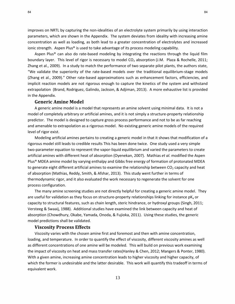
13

improves on NRTL by capturing the non-idealities of an electrolyte system primarily by using interaction

parameters, which are shown in the Appendix. The system deviates from ideality with increasing amine

concentration as well as loading, as both lead to a greater concentration of electrolytes and increased

ionic strength. Aspen Plus® is used to take advantage of its process modeling capability.

Aspen Plus® can also do rate-based modeling by integrating the reactions through the liquid film

boundary layer. This level of rigor is necessary to model CO2 absorption (J.M. Plaza & Rochelle, 2011;

Zhang et al., 2009). In a study to match the performance of two separate pilot plants, the authors state,

“We validate the superiority of the rate-based models over the traditional equilibrium-stage models

(Zhang et al., 2009).” Other rate-based approximations such as enhancement factors, efficiencies, and

implicit reaction models are not rigorous enough to capture the kinetics of the system and withstand

extrapolation (Brand, Rodriguez, Galindo, Jackson, & Adjiman, 2013). A more exhaustive list is provided

in the Appendix.

Generic Amine Model A generic amine model is a model that represents an amine solvent using minimal data. It is not a

model of completely arbitrary or artificial amines, and it is not simply a structure-property relationship

predictor. The model is designed to capture gross process performance and not to be as far reaching

and amenable to extrapolation as a rigorous model. No existing generic amine models of the required

level of rigor exist.

Modeling artificial amines pertains to creating a generic model in that it shows that modification of a

rigorous model still leads to credible results This has been done twice. One study used a very simple

two-parameter equation to represent the vapor-liquid equilibrium and varied the parameters to create

artificial amines with different heat of absorption (Oyenekan, 2007). Mathias et al. modified the Aspen

Plus® MDEA amine model by varying enthalpy and Gibbs free energy of formation of protonated MDEA

to generate eight different artificial amines to examine the relationship between CO2 capacity and heat

of absorption (Mathias, Reddy, Smith, & Afshar, 2013). This study went further in terms of

thermodynamic rigor, and it also evaluated the work necessary to regenerate the solvent for one

process configuration.

The many amine screening studies are not directly helpful for creating a generic amine model. They

are useful for validation as they focus on structure-property relationships linking for instance pKa or

capacity to structural features, such as chain length, steric hindrance, or hydroxyl groups (Singh, 2011;

Versteeg & Swaaij, 1988). Additional studies have examined the link between capacity and heat of

absorption (Chowdhury, Okabe, Yamada, Onoda, & Fujioka, 2011). Using these studies, the generic

model predictions shall be validated.

Viscosity Process Effects Viscosity varies with the chosen amine first and foremost and then with amine concentration,

loading, and temperature. In order to quantify the effect of viscosity, different viscosity amines as well

as different concentrations of one amine will be modeled. This will build on previous work examining

the impact of viscosity on heat and mass transfer rates(Hanley & Chen, 2012; Mangers & Ponter, 1980).

With a given amine, increasing amine concentration leads to higher viscosity and higher capacity, of

which the former is undesirable and the latter desirable. This work will quantify this tradeoff in terms of

equivalent work.

84 84

14

A first step has been taken for the cross exchanger (L. Li, Voice, et al., 2013). The cost to heat the

solvent can be broken into capital (area A$) and operating (sensible heat translated into an equivalent

work W$), and this can be used to find ΔTopt, an optimal temperature difference.

(1)

Using the Colburn equation (Incropera, 2006), the heat transfer coefficient h is related to viscosity µ by

(2)

Combining this relationship with the cost relationship, solvents can be ranked according to

(3)

where ΔC is capacity (mol CO2/kg solvent), ΔCµ is viscosity-normalized capacity (mol CO2/kg solvent), and µαmid

(cP)is the viscosity at the middle of the loading range. This work will improve upon Equation 1 by

including pressure drop. This metric ΔCµ is helpful for preliminarily ranking the solvents by viscosity. The next step will be to

look at viscosity effects in the absorber, where it changes mass transfer by lowering kl, the liquid mass

transfer coefficient, decreasing diffusion coefficients of amine and products, and altering effective area

(Tsai, 2010).

Economic Evaluation Being able to compare many different process configurations and solvents directly on a dollars-to-

dollars basis is necessary to determine the best design. Economic calculations are inherently error

prone due to their dependence on location- and time-sensitive parameters. So while rigorous economic

calculations are beneficial for actually constructing an amine scrubber, from the perspective of

understanding the cost centers, a single economic heuristic will suffice. This dissertation seeks to

develop that heuristic.

As with previous economic evaluations of amine scrubbing, we will also focus on one amine and one

process configuration, most likely an advanced stripper configuration with intercooling in the middle of

the absorber (Abu-Zahra, Schneiders, Niederer, Feron, & Versteeg, 2007; Desideri & Paolucci, 1999; Mac

Dowell & Shah, 2013; Nuchitprasittichai & Cremaschi, 2011; Trimeric Corporation, 2005). Additionally,

many of these evaluations neglect cost-centers by ignoring compression cost or are flawed by being

based on only equilibrium reactions. The economic heuristic to be developed would overcome both of

these flaws.

There have been prior efforts to develop consistent costing methodology. Each effort offers its own

set of guidelines for costing the process (contingency, interest during construction, etc), however they

all conflict on the values assigned (DOE, 2005; IEAGHG, 2013; NETL, 2013). This is due to different base

years and locations for which the models were developed. These studies will be consulted for guidance

in costing equipment and checking predicted costs.

Methods and Preliminary Results

Rigorous Thermodynamic and Kinetic Models

85 85

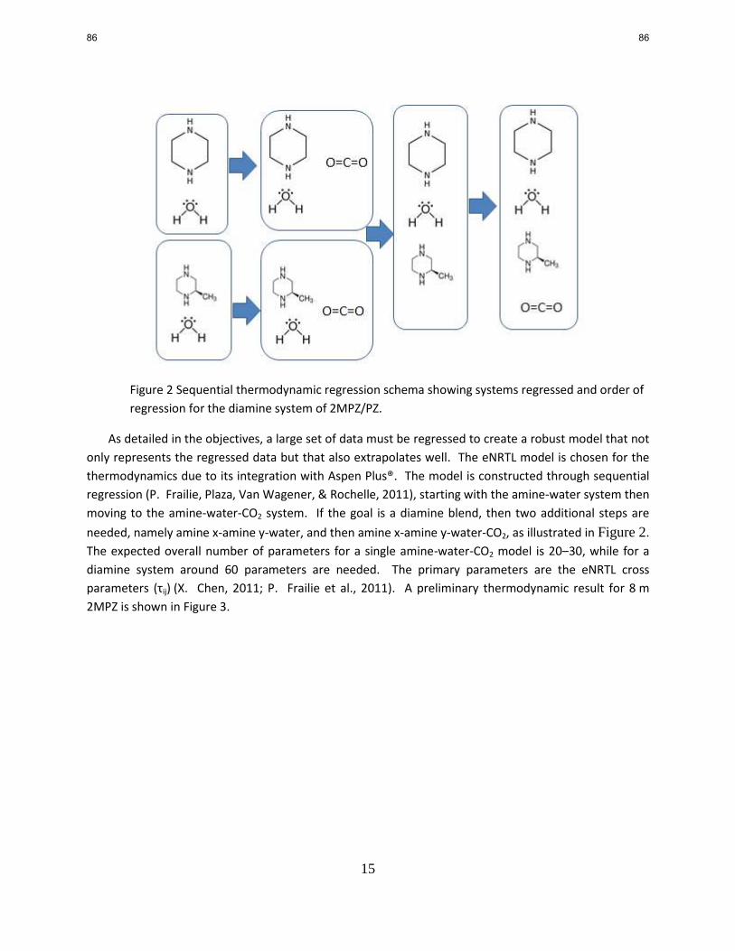
15

Figure 2 Sequential thermodynamic regression schema showing systems regressed and order of

regression for the diamine system of 2MPZ/PZ.

As detailed in the objectives, a large set of data must be regressed to create a robust model that not

only represents the regressed data but that also extrapolates well. The eNRTL model is chosen for the

thermodynamics due to its integration with Aspen Plus®. The model is constructed through sequential

regression (P. Frailie, Plaza, Van Wagener, & Rochelle, 2011), starting with the amine-water system then

moving to the amine-water-CO2 system. If the goal is a diamine blend, then two additional steps are

needed, namely amine x-amine y-water, and then amine x-amine y-water-CO2, as illustrated in Figure 2.

The expected overall number of parameters for a single amine-water-CO2 model is 20‒30, while for a

diamine system around 60 parameters are needed. The primary parameters are the eNRTL cross

parameters (τij) (X. Chen, 2011; P. Frailie et al., 2011). A preliminary thermodynamic result for 8 m

2MPZ is shown in Figure 3.

86 86

16

Figure 3 CO2 solubility of 8 m 2MPZ. Curves are the model, while filled points are WWC and open points

total pressure (X. Chen, 2011; Xu, 2011).

The thermodynamic and kinetic models are intimately linked through speciation which is governed

by reaction equilibrium constants. All of the models mentioned in previous section used a polynomial

expression to calculate these constants. This resulted in using two sets of fG ,

fH , and

PC values

to calculate thermodynamic properties and equilibrium constants. If these two sets differ, there is a

thermodynamic inconsistency, which is usually manifested in unusual heat capacity behavior. For this

reason, the equilibrium constants are calculated using Equation 4 to ensure that the same set of fG ,

fH , and

PC values is used throughout the model.

dTR

CdT

R

C

TRT

H

RT

HG

RT

GK

T

T

P

T

T

Peq

00

1ln 0

0

00

(4)

Assured of consistent thermodynamics, the kinetic model may proceed. The goal of kinetic

modeling is to match wetted wall column (WWC) data by varying the reaction pre-exponential (ko),

activation energy (EA), and the diffusivity of products and reactants (α and β of Equation 6) (X. Chen,

2011). As viscosity is involved in the calculation of diffusivity, it is regressed first. Then, the density is

regressed to allow for converting from volumetric flow rates to mass flow rates. Once the hydraulics are

done, the reaction parameters are regressed.

1.E+00

1.E+01

1.E+02

1.E+03

1.E+04

1.E+05

1.E+06

1.E+07

0 0.1 0.2 0.3 0.4 0.5

P*CO2

(Pa)

Loading (mol CO2/mol alk)

100 °C

20 °C 40 °C

80 °C

60 °C

120 °C

140 °C

160 °C

87 87

17

Figure 4 Kinetic modeling flow sheet.

As with all regressions, fewer parameters give a more stable result, and so to minimize the number

of parameters, the fewest reactions possible are used to match the experimental flux of CO2. To further

reduce the number of parameters, only one or two reactions are chosen to be regressed, while the

others are ratioed using a Brønsted plot (Cullinane, 2005). All reversible reactions are represented using

a power law, shown in Equation 5, with separate forward and reverse reactions.

(5)

(6)

where k0 is the reaction pre-exponential, EA is the activation energy, R is the universal gas constant, and

Tref is the reference temperature. Do, β, and α are adjustable parameters.

At higher temperatures, the diffusivity becomes more limiting, and so the parameters of Equation 6

are regressed. Once everything has been regressed, the model is checked. If needed, another iteration

is performed, as sketched in Figure 4. Once the thermodynamic data is well matched, and predicted

fluxes are within 20% of experimental fluxes, process simulation can take place.

Generic Amine Model

88 88

18

Figure 5 CO2 solubility of 4 m 2MPZ/4 m PZ. Curves are the model; filled points WWC (X. Chen,

2011); open points total pressure (Xu, 2011).

To create a generic amine model, an existing rigorous Aspen Plus® model is adapted using minimal

experimental data, maybe as few as three CO2 solubility data points. (A full list of basis rigorous models

is provided in the Appendix.) The most similar amine model is selected as a basis, and then CO2 solubility

are fit using the eNRTL cross parameters as well as Gibbs free energy of select amine species. These

data determine capacity and heat of absorption, making their accurate representation critical to

matching process performance. If the thermodynamic model fit is well and the other predicted

properties are reasonable, the kinetics are adjusted to match WWC flux data. This will be done by

adjusting existing reaction parameters.

It is important to keep in mind the limitations of this model. It will not extrapolate well, and many

properties of potential interest will not be regressed but rather simply rely on the basis rigorous model.

However, the benefits of quickly crafting a model to capture gross process performance outweigh these

drawbacks, and these drawbacks can be dealt with by collecting more data for fitting.

As a first step towards this generic model, a preliminary thermodynamic model for 2MPZ/PZ was

created by modifying the pure PZ model using the above procedure. This model matches the CO2

solubility data as shown in Figure 5.

Viscosity Process Effects Viscosity effects on process design will be explored in two ways. One is by comparing a high

viscosity and a low viscosity solvent, such as 7 m MEA and 8 m 2MPZ. The second is by comparing one

solvent at different concentrations, such as 5 m and 8 m 2MPZ. In this exploration, the same process

configuration will be used and its equipment will be sized. Particular attention will be paid to the size of

40 °C

60 °C 80 °C

100 °C 120 °C

140 °C

160 °C

1.E+00

1.E+01

1.E+02

1.E+03

1.E+04

1.E+05

1.E+06

1.E+07

1.E+08

0 0.1 0.2 0.3 0.4 0.5

P*CO2

(Pa)

Loading (mol CO2/mol alk)

CO2 Solubility

89 89

19

the heat exchanger—as increased viscosity decreases heat transfer rates—and the amount of packing in

the absorber—as increased viscosity decreases mass transfer rates. The results of this exploration will

guide future work in this area, but at a minimum one other process configuration will be examined to

determine if viscosity is a deciding factor in process design.

Economic Evaluation The first step will be to determine a representative base case process model that applies to all

solvents of interest. Most likely this will be a simple stripper and an intercooled absorber, which will be

the same configuration used for the viscosity studies. With a base case established, the equipment can

be sized. Most sizing rules are well established, but the heat exchanger has historically given trouble.

For this reason, new methods of sizing the heat exchanger will be trialed.

With this foundation laid, an exploration of different amines and amine concentrations can be done.

This will test the sizing rules and allow for refinement, while at the same time leading to a greater

understanding of capital and operating expense tradeoffs, especially as shown in packing area and

equivalent work. Using this exploration and the spreadsheet model developed by Peter Frailie, an

economic heuristic will be developed to allow for quick estimation of total capital expenditure.

Essentially, the rigorous financial and equipment costing models will be reduced down to one equation

for the total annualized cost (TAC) using purchased equipment cost (PEQ) and energy of the form:

CenergyBPEQATAC (7)

TimelineFall 2013

2MPZ model completion

2MPZ/PZ model completion (paper)

model comparison for generic model

Spring 2014

AMP/PZ model completion (paper)

viscosity sensitivity analysis for 5 m and

8 m 2MPZ

generic model development

Fall 2014

generic model completion (oral

presentation and paper for GHGT-12)

viscosity study comparing a high and a

low viscosity solvent

Spring 2015

economic heuristic development

generic model validation

Fall 2015

economic heuristic completion (paper)

process simulation using generic

models

Spring 2016

dissertation write up

graduation

90 90

20

References

Abu-Zahra, M. R. M., Schneiders, L. H. J., Niederer, J. P. M., Feron, P. H. M., & Versteeg, G. F. (2007). CO2 capture from power plants. International Journal of Greenhouse Gas Control, 1(1), 37–46. doi:10.1016/S1750-5836(06)00007-7

Austgen, D. (1989). A Model of Vapor-Liquid Equilibriua for Acid Gas-Alkanolamine-Water Systems. The University of Texas at Austin.

Bishnoi, S., & Rochelle, G. T. (2000). Absorption of carbon dioxide into aqueous piperazine: reaction kinetics, mass transfer and solubility. Chemical Engineering Science, 55(22), 5531–5543. doi:10.1016/S0009-2509(00)00182-2

Brand, C. V, Rodriguez, J., Galindo, A., Jackson, G., & Adjiman, C. S. (2013). Validation of a process model of CO2 capture in an aqueous solvent , using an implicit molecular based treatment of the reactions, 00, 1–6.

Chen, C.-C., Britt, H. I., Boston, J. F., & Evans, L. B. (1982). Local Composition Model for Excess Gibbs Energy of Electrolyte Systems. AIChE Journal, 28(4), 588–596.

Chen, C.-C., & Song, Y. (2004). Generalized electrolyte-NRTL model for mixed-solvent electrolyte systems. AIChE Journal, 50(8), 1928–1941. doi:10.1002/aic.10151

Chen, X. (2011). Carbon Dioxide Thermodynamics, Kinetics, and Mass Transfer in Aqueous Piperazine Derivatives and Other Amines. The University of Texas at Austin.

Chowdhury, F. A., Okabe, H., Yamada, H., Onoda, M., & Fujioka, Y. (2011). Synthesis and selection of hindered new amine absorbents for CO2 capture. Energy Procedia, 4, 201–208. doi:10.1016/j.egypro.2011.01.042

Cullinane, J. T. (2005). Thermodynamics and Kinetics of Aqueous Piperazine with Potassium Carbonate for Carbon Dioxide Absorption. The University of Texas at Austin.

Desideri, U., & Paolucci, A. (1999). Performance modelling of a carbon dioxide removal system for power plants. Energy Conversion and Management, 40(18), 1899–1915. doi:10.1016/S0196-8904(99)00074-6

DOE. (2005). Carbon Capture and Sequestration Systems Analysis Guidelines (p. 67).

Dugas, R. E. (2009). Carbon Dioxide Absorption , Desorption , and Diffusion in Aqueous Piperazine and Monoethanolamine. The University of Texas at Austin.

Edali, M., Idem, R., & Aboudheir, A. (2010). 1D and 2D absorption-rate/kinetic modeling and simulation of carbon dioxide absorption into mixed aqueous solutions of MDEA and PZ in a laminar jet apparatus. International Journal of Greenhouse Gas Control, 4(2), 143–151. doi:10.1016/j.ijggc.2009.11.005

91 91

21

EPA. (2009). Endangerment and Cause or Contribute Findings for Greenhouse Gases Under Section 202 (a) of the Clean Air Act. earth1.epa.gov. Retrieved from http://earth1.epa.gov/climatechange/Downloads/endangerment/rtc_volume_3.pdf

Ermatchkov, V., & Pe, Ä. (2006). Solubility of Carbon Dioxide in Aqueous Solutions of N-Methyldiethanolamine in the Low Gas Loading Region, 6081–6091.

Frailie, P., Plaza, J., Van Wagener, D., & Rochelle, G. T. (2011). Modeling piperazine thermodynamics. Energy Procedia, 4, 35–42. doi:10.1016/j.egypro.2011.01.020

Hanley, B., & Chen, C. (2012). New mass transfer correlations for packed towers. AIChE journal, 58(1). doi:10.1002/aic

IEAGHG. (2013). Criteria for Technical and Economic Assessment of Plants with Low CO2 Emissions.

Incropera, F. P. (2006). Fundamentals of Heat and Mass Transfer (6th ed.). Wiley.

Intergovernmental Panel on Climate Change (IPCC) (2005). Summary for Policymakers of the Intergovernmental Panel on Climate Change.

International Energy Agency (IEA) (2008). Energy Technology Perspectives.

International Energy Agency (IEA) (2010). Carbon capture and storage. Energy Policy. Retrieved from http://www.sciencedirect.com/science/article/pii/S0301421508004436

International Energy Agency (IEA) (2011). CO2 Emissions from Fuel Combustion 2011 (p. 133). OECD Publishing. doi:10.1787/co2_fuel-2011-en

Kohl, A., & Nielsen, R. (1997). Gas Purification (5th ed., p. 1395). Houston: Gulf Professional Publishing.

Li, H., Li, L., Nguyen, T., Rochelle, G. T., & Chen, J. (2013). Characterization of Piperazine / 2-Aminomethylpropanol for Carbon Dioxide Capture, 00, 1–13.

Li, L., Li, H., Namjoshi, O., Du, Y., & Rochelle, G. T. (2013). Absorption rates and CO2 solubility in new piperazine blends, 00, 1–16.

Li, L., Voice, A. K., Li, H., Namjoshi, O., Nguyen, T., Du, Y., & Rochelle, G. T. (2013). Amine blends using concentrated piperazine. Energy Procedia.

Mac Dowell, N., & Shah, N. (2013). Identification of the cost-optimal degree of CO2 capture: An optimisation study using dynamic process models. International Journal of Greenhouse Gas Control, 13, 44–58. doi:10.1016/j.ijggc.2012.11.029

Mangers, R., & Ponter, A. (1980). Effect of viscosity on liquid film resistance to mass transfer in a packed column. Industrial & Engineering Chemistry …, 530–537. Retrieved from http://pubs.acs.org/doi/abs/10.1021/i260076a005

92 92

22

Mathias, P. M., Reddy, S., Smith, A., & Afshar, K. (2013). A Guide to Evaluate Solvents and Processes for Post-Combustion CO2 Capture, 00, 1–8.

NETL. (2013). Capital Cost Scaling Methodoloy.

Nuchitprasittichai, A., & Cremaschi, S. (2011). Optimization of CO2 capture process with aqueous amines using response surface methodology. Computers & Chemical Engineering, 35(8), 1521–1531. doi:10.1016/j.compchemeng.2011.03.016

Oyenekan, B. (2007). Modeling of Strippers for CO2 Capture by Aqueous Amines. The University of Texas at Austin.

Plaza, J.M., & Rochelle, G. T. (2011). Modeling pilot plant results for CO2 capture by aqueous piperazine. Energy Procedia, 4, 1593–1600. Retrieved from http://www.sciencedirect.com/science/article/pii/S1876610211002268

Plaza, Jorge M. (2011). Modeling of Carbon Dioxide Absorption using Aqueous Monoethanolamine, Piperazine and Promoted Potassium Carbonate. The University of Texas at Austin.

Rochelle, G. T. (2009). Amine scrubbing for CO2 capture. Science (New York, N.Y.), 325(5948), 1652–4. doi:10.1126/science.1176731

Singh, P. (2011). Amine Based Solvent for CO2 Absorption “From Molecular Structure to Process”. University of Twente.

Song, Y., & Chen, C.-C. (2009). Symmetric Electrolyte Nonrandom Two-Liquid Activity Coefficient Model. Industrial & Engineering Chemistry Research, 48(16), 7788–7797. doi:10.1021/ie9004578

Trimeric Corporation. (2005). Integrating MEA Regeneration with CO2 Compression and Peaking to Reduce CO2 Capture Costs. Power.

Tsai, R. (2010). Mass Transfer Area of Structured Packing. The University of Texas at Austin.

U. S. Energy Information Administration (2012a). Short-term energy outlook (p. 44). Retrieved from http://www.osti.gov/energycitations/product.biblio.jsp?osti_id=6030138

U. S. Energy Information Administration (2012b). AEO2012 Early Release Overview, 2012, 1–13.

Versteeg, G., & Swaaij, W. van. (1988). On the kinetics between CO2 and alkanolamines both in aqueous and non-aqueous solutions—II. Tertiary amines. Chemical engineering science, 43(3), 587–591. Retrieved from http://www.sciencedirect.com/science/article/pii/0009250988870180

Xu, Q. (2011). Thermodynamics of CO2 Loaded Aqueous Amines. University of Texas at Austin.

Zhang, Y., & Chen, C.-C. (2011). Thermodynamic Modeling for CO2 Absorption in Aqueous MDEA Solution with Electrolyte NRTL Model. measurements, 163–175. Retrieved from http://www.aspentech.com/downloads/thermodynamic_modeling_co2.pdf

93 93

23

Zhang, Y., Chen, H., & Chen, C. (2009). Rate-based process modeling study of CO2 capture with aqueous monoethanolamine solution. Industrial & …, 9233–9246. Retrieved from http://pubs.acs.org/doi/abs/10.1021/ie900068k

Zhang, Y., Que, H., & Chen, C.-C. (2011). Thermodynamic modeling for CO2 absorption in aqueous MEA solution with electrolyte NRTL model. Fluid Phase Equilibria, 311, 67–75. doi:10.1016/j.fluid.2011.08.025

Zong, L., & Chen, C.-C. (2011). Thermodynamic modeling of CO2 and H2S solubilities in aqueous DIPA solution, aqueous sulfolane–DIPA solution, and aqueous sulfolane–MDEA solution with electrolyte NRTL model. Fluid Phase Equilibria, 306(2), 190–203. doi:10.1016/j.fluid.2011.04.007

Disclaimer: This presentation was prepared as an account of work sponsored by an agency of

the United States Government. Neither the United States Government nor any agency

thereof, nor any of their employees, makes any warranty, express or implied, or assumes

any legal liability or responsibility for the accuracy, completeness, or usefulness of any

information, apparatus, product, or process disclosed, or represents that its use would not

infringe privately owned rights. Reference herein to any specific commercial product,

process, or service by trade name, trademark, manufacturer, or otherwise does not

necessarily constitute or imply its endorsement, recommendation, or favoring by the United

States Government or any agency thereof. The views and opinions of authors expressed

herein do not necessarily state or reflect those of the United States Government or any

agency thereof.

Appendix

94 94

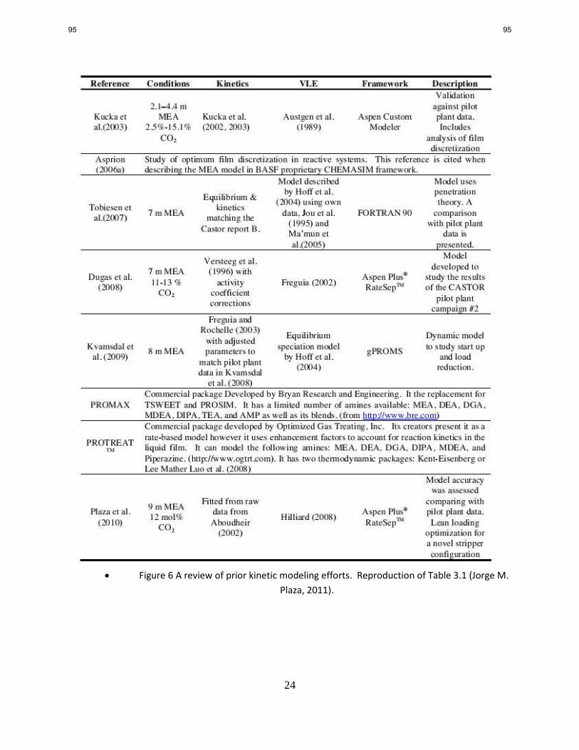
24

Figure 6 A review of prior kinetic modeling efforts. Reproduction of Table 3.1 (Jorge M.

Plaza, 2011).

95 95

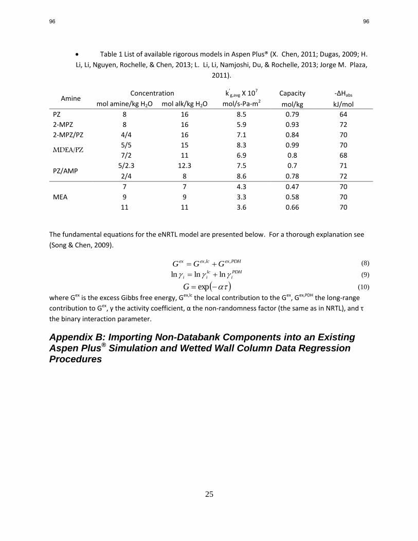
25

Table 1 List of available rigorous models in Aspen Plus® (X. Chen, 2011; Dugas, 2009; H.

Li, Li, Nguyen, Rochelle, & Chen, 2013; L. Li, Li, Namjoshi, Du, & Rochelle, 2013; Jorge M. Plaza,

2011).

Amine Concentration k’

g,avg X 107 Capacity -ΔHabs

mol amine/kg H2O mol alk/kg H2O mol/s-Pa-m2 mol/kg kJ/mol

PZ 8 16 8.5 0.79 64

2-MPZ 8 16 5.9 0.93 72

2-MPZ/PZ 4/4 16 7.1 0.84 70

MDEA/PZ 5/5 15 8.3 0.99 70

7/2 11 6.9 0.8 68

PZ/AMP 5/2.3 12.3 7.5 0.7 71

2/4 8 8.6 0.78 72

MEA

7 7 4.3 0.47 70

9 9 3.3 0.58 70

11 11 3.6 0.66 70

The fundamental equations for the eNRTL model are presented below. For a thorough explanation see

(Song & Chen, 2009).

PDHexlcexex GGG ,, (8)

PDH

i

lc

ii lnlnln (9)

expG (10)

where Gex is the excess Gibbs free energy, Gex,lc the local contribution to the Gex, Gex,PDH the long-range

contribution to Gex, γ the activity coefficient, α the non-randomness factor (the same as in NRTL), and τ

the binary interaction parameter.

Appendix B: Importing Non-Databank Components into an Existing Aspen Plus® Simulation and Wetted Wall Column Data Regression Procedures

96 96

26

Importing Non-Databank Components into an Existing Aspen Plus® Simulation Purpose: This procedure is useful for merging two existing Aspen thermodynamic models . It was

developed for the creation of 2MPZ/PZ blend model by merging 2MPZ into the Independence

model.

Created: 2013-06-12 by Brent Sherman

Modified: 2013-6-24 by Brent Sherman

It is best to merge the models in as few as sittings as possible. The reason is there are many different

things that need to be changed, and these are scattered throughout the Aspen interface. Failure to

update all of them will lead to cryptic error messages that will lead you in the wrong direction.

Throughout this procedure, I will refer to pulling from a source model. This is the model that has the

components you want to merge into the other model. The other model I’ll call the destination model.

Add the New Components Under ComponentsSpecification in the source model, right click and copy and paste

each component one-by-one into the destination model.

o with each paste, click User Defined in both simulations. I make sure the Aliases

match, and the properties on the Conventional Component Basic Data sheet

(the next page) match, and lastly that the Conventional Component

Additional Data also match.

add the amine and zwitterion to the list of Henry’s components: ComponentsHenry

CompsHC-1

Change the Parameters Now, begin to change all the parameters. In all cases, you will look at the source model and change the

destination model parameters to match. First, change the scalar parameters.

Use PropertiesPure ComponentUSRDEF to change non-temperature dependent

parameters. Watch out as the default unit may conflict with the retrieve parameter unit.

Then start changing the temperature dependent parameters

o If a T-dependent parameter is not showing, select

PropertiesParametersPure Component and click New… .

o Add the amine to THRSWT-1: ParameterPure ComponentTHRSWT-1

The flags here are critical. They determine what property methods are used to

calculate all of the basic thermo properties (critical T and P, compressibility, Cp,

etc)

Similarly, the flags in TRNSWT-1 select the transport submodels used.

97 97

27

Once all the pure component ones are changed, change the Binary Interaction

parameters.

o Henry, NRTL, and VLCLK.

Then do the Electrolyte Pair parameters.

o Cut and paste the GMELCC, GMELCD, and GMELCE values.

Verify Parameters In both simulations, use ToolsRetrieve Parameter Results to see all parameters

for the components of interest.

o Put these into Excel, mark the ones that are different, and start making them match up

o Keep track of what has been changed as Aspen doesn’t always take the first change

(unpredictable and non-reproducible, so be scrupulous and double check)

When you think you are done, retrieve parameter results and check again.

o Error-prone as cutting and pasting can truncate accidentally.

o Easy to lose track of parameters in the sea of numbers.

o Easy to forget to change units.

Check which parameters are actually used by looking at the switches in THRSTW-1 and

TRNSWT-1.

Update Chemistry You must copy over the equilibrium reactions in order for the system to speciate. Don’t forget

to do both GLOBAL and REDUCED.

If you fail to do so and attempt to calculate the properties for components that are not present

(ie you add the amine and try to calculate the related species’ properties), you will see the

following error, “EOS LIQUID VOLUME CALCULATION FAILED TO CONVERGE

AFTER 99 ITERATIONS”.

If your source model has kinetic reactions, copy those as well.

Update Subroutines You must merge each subroutine. This will involve adding in new variables, if switches, and

other code.

o vl2u2.f

o mul2u2.f

o dl0u.f

Verify Thermodynamic Integrity The best way to verify proper behavior is through Property Analysis blocks.

Before copying and pasting the property analysis blocks over, you need to copy and paste the

Prop-Sets.

Now copy and paste over the Analysis blocks.

o gamma

o heat of absorption

o pKa

o density

o speciation

o vapor pressure

98 98

28

When it’s all done, verify that you have achieved the same performance that you previously

had.

Remember that for pKa, you need to use the chemistry that includes protons.

Wetted Wall Column Data Regression Purpose: To match the experimental flux within ±20% by changing rate constants and the effective

diffusion coefficient of reactants and products.

Created: 2012-06-25 by Brent Sherman

Last Updated: 2013-06-27 by Brent Sherman

Prerequisites Subroutines

o area (area.obj)

o diffusivity (dl0u.obj)

o pressure drop (pressuredrop.obj)

o density (vl2u2.obj)

o viscosity (mul2u2.obj)

o bubble point (drusr0.obj)

o mass transfer (masstransfer.obj)

Raw data from the WWC (one .xlsx file for each loading and temp. combo)

An Excel workbook for pre- and post-processing.

Complete thermo model

Complete hydraulic model (vl2u2 and mul2u2 must be current)

Method

Raw Data Pre-processing While processing the data, check the experimental fit. Do any of the points seem to be outliers? Is the

line straight and through the origin? What would cause these things?

Extract the raw experimental data from the Excel files supplied by the experimenter.

o There are three sheets in each file: Sheet1, Gas Film Resistance, and Gas Mixtures.

Regression data is in the first two sheets.

Be careful of the units and diameter scaling, as this will change the flux values.

From the first, take the fluxes, Ptotal, P*CO2, and Qtotal.

From the second, take Qgas (both values), kg, kg’, and Kg

o This data should go in the provided Excel template, which looks like below. There is far

more to the spreadsheet than that shown below.

99 99

29

o All of the data extracted is put into one large table whence many more things are

calculated. Check molecular weights.

o This data is preprocessed and sent to another table for input into Aspen with the proper

units.

o Check the diameter of the WWC and rescale as necessary. The WWC is either 10x or

100x the physical diameter.

Aspen Simulation

Figure 7 Aspen WWC PFD.

Description

In the above figure are the WWC and two flash blocks. The rich and lean flash blocks simply flash the

rich and lean solvents in a bubble point calculation to determine the equilibrium partial pressure of CO2.

The lean solvent is fed in three separate streams to a mixer. The heat of mixing and speciation is then

dealt with using the heater block. The vapor stream contains N2 and CO2. This feed gas and a liquid

100 100

30

water stream go to the saturator, which is a T-P flash block. This process ensures the liquid and vapor

feeds are isothermal with the WWC itself.

The WWC is a three stage RADFRAC column. Its diameter is 10 or 100x the actual WWC diameter, but

the height is the same (9.1 cm). The WWC uses the counter-current flow model with a discretized liquid

film and 5% liquid hold up. It uses a customized mass transfer and interfacial area subroutine, rendering

the choice of packing irrelevant.

There are three calculator blocks used. C-LDGS simply checks the loadings to make sure they are as they

should be. C-FLUX computes the flux and KG, the overall gas side mass transfer coefficient. C-KEQ

calculates the equilibrium constants for each reaction, ratios the rates of reaction, and back-calculates

the reverse rates of reaction. For the sake of this block, all activation energies are set to 0, which

reduces kr to kf/Keq.

Method: Generating a set of ko’s and EA’s

Pick two points at 40 and 60 °C.

o one dominated by the bicarbonate reaction

o one dominated by the carbamate

Note that practically speaking, the carbamate is the most significant reaction

across the whole range as it is the fastest reaction.

Cut and paste all flowrates from Excel into Aspen.

Update the temperature and pressure of the 2MPZ stream. The transfer blocks will propagate

these throughout the model.

In the reaction set, make sure all activation energies are set to 0.

Adjust loading to give the same error in the absorption and desorption points.

o Always re-initialize before each run.

o Run with a fixed set of ko’s and EA’s.

o Start with the experimental loading if you have no better guess.

o Run the simulation and calculate the ratio of the predicted flux to the experimental flux.

o Run until the difference beteen the ratios is less than 1% or you have adjusted the

loading as much as possible.

o Don’t be afraid if the ratio is poor, and the loading is maximally adjusted. This process is

iterative, and the results will improve over time.

Adjusting loading notes

o Make sure the design spec and the KEQ calculator block are disabled, as both change ko

values.

o only adjust 10% of the operational loading range (this works out to 0.01 mol/mol alk. for

2MPZ)

o The idea behind this is that at 0 driving force, there should be zero flux. Thus having the

same over- or under-prediction for both points will ensure the line goes through the

origin.

101 101

31

o Setting the activation energies to zero makes the reaction pre-exponential equal to the

rate of reaction.

o You will always use adjusted loading values for Aspen.

Now, run the regression using the adjusted loading to get k values.

o Activate the design spec and the KEQ calculator block.

o Run it for the desorption points at high loading. Record KEQ‘s and kf.

arbitrary decision to use high loading desorption points

o Input the experimental flux into the design spec as you run each point.

o Set the design spec to vary one of the forward ko’s. Record the result.

o Then rerun varying the other ko’s.

You should be able to perfectly match the flux.

o Then repeat for the second temperature.

o Back calculate kr from KEQ and kf.

o You should now have for each reaction a KEQ, a kf, and a kr.

Calculate the activation energies.

o Use goal seek to solve the following equation by varying EA.

o C

ref

AC k

TTR

Ek 6040

110

o Ratioed reactions will have the same activation energy as the reaction they are ratioed

to.

o It’s a good idea to double check that using the ko and EA calculated, you duplicate the k

at 60C.

o Repeat this procedure for the reverse reactions.

You now have a set of ko’s and EA’s that are thermodynamically consistent. Fix these. Turn off

the design spec and the KEQ calculator block.

From here on out, you will simply be repeating the loading adjustment calculation.

Tref 3.13E+02 K

R 8.31E+00 J/mol-K

run for the high loading points

Regressed

using desorption

forward

Rxn # KEQ kf kr Rxn EA

goal seek f

kf 60 check

313.15

1 7.13E+00 2.14E+09 3.00E+08 1 7.27E+04 1.51E-04 1.14E+10

2 3.67E+05 3.60E+11 9.80E+05 2 -

1.25E+05 0.00E+00 2.03E+10

3 4.71E+01 3.16E+11 6.71E+09 3 -

1.25E+05 0.00E+00 1.79E+10

333.15

1 1.23E+00 1.14E+10 9.30E+09 2 6.38E+04 2.03E+10 3.19E+05 3 3.98E+00 1.79E+10 4.49E+09 Figure 8 Sample of regression excel sheet.

102 102

32

Method: Checking the Fit

Now, repeat the loading adjustment for all of the data points using the fixed set of ko’s and EA’s.

Adjust the loadings until the under- or over-prediction is less than 1%. However, do not adjust

more than 10% of the operational loading range.

Plot the data vs T and loading. Look for trends indicating systematic bias. Sample plots are

shown below.

Figure 9 8 m 2MPZ kinetic fit.

0.6

1.0

1.4

1.8

Fluxpred/ Fluxexp


40 abs 40 des

60 abs 60 des

80 abs 80 des

100 abs 100 des

103 103

33

Figure 10 8 m 2MPZ kinetic fit.

Method: Starting a New Iteration You checked your data, and there is a trend. Or there is no trend, but you simply want a tighter fit. You

can regress reaction rate constants or diffusion parameters.

Changing the reaction rate

o change the ko as you please

o repeat the loading adjustment for the same two data points previously used

o repeat the regression step

o then, fix the ko’s and EA’s and run through all the data points repeating the loading

adjustment

Changing the diffusion parameters

o no need to the re-regress ko’s and EA’s

o simply run back through the data, repeating the loading adjustment

Appendix C: CCSI IAB Meeting April 2013 Posters

0.6

1.0

1.4

1.8

40 60 80 100

Fluxpred/ Fluxexp

T (°C)

40 abs 40 des

60 abs 60 des

80 abs 80 des

100 abs 100 des

104 104

34

105 105

35

106 106

1

Dynamic Modeling and Control of Amine Scrubbing


by Matthew Walters




July 31, 2013

Abstract

A dynamic model of solvent regeneration using piperazine is being developed in gPROMS®

. To

improve the quality of the code and reduce the chance of mistakes, all of the thermophysical

properties of the amine solvent have been compiled into one dynamic link library file.

gPROMS® interfaces with this user defined properties package by treating it as a foreign object.

The previously developed model of a separator vessel has been modified to account for vapor

inventory, since this may affect the transient behavior of the system. The goal of creating a

dynamic model is for the development of process control strategies. The major process control

objectives for amine scrubbing have been identified: reject disturbances from the upstream

power plant, track set point changes made in response to grid demand, obey process constraints,

and allow for stable operation with process intensification. A multiple time scale behavior is

demonstrated, which suggests the need for a hierarchical controller design.

Introduction

Dynamic models are useful tools for designing process control strategies, optimizing off-design

steady state conditions, and understanding the system response to input changes or disturbances.

Several models have been developed and validated to predict the steady state operation of amine

scrubbing (see review by Wang et al., 2011). However, there are only a few examples of works

concerned with the dynamics of this process (Kvamsdal et al., 2009; Lawal et al., 2009;

Tobieson et al., 2012; Ziaii, 2012). A major objective of this research is to develop and validate

a detailed equation-based dynamic model of an amine scrubbing plant using piperazine (PZ)

solvent and advanced process configurations. Another objective is to use the model to develop a

process control strategy that satisfies process constraints as well as economic objectives. The

strategy should be effective in the presence of model and parameter uncertainty. This research

strives to address some of the challenges associated with process design and control so that

recommendations may ultimately be made for the operation of carbon capture from commercial

scale power plants.

Thermophysical Properties Package for Piperazine

Process flowsheeting software, such as Aspen Plus® or gPROMS

®, generally provides a

thermophysical properties library which allows the user to perform equilibrium calculations for

chemical compounds available in its database. In the case of amine-H2O-CO2 systems,

107 107

2

properties calculated from the built-in libraries do not provide adequate agreement with

experimental data to accurately simulate an amine scrubbing process. It therefore becomes

necessary to either modify the existing thermophysical properties package (for example see

Frailie et al., 2011) or to create a custom package which is consistent with the experimental

results. In gPROMS®, the best way to include equation-based thermophysical properties for an

amine scrubbing system is through developing an independent properties library for the desired

amine solvent. gPROMS® can then call this library without having to repeatedly include the

same set of equations in the model of each individual unit operation. Additionally, the unit

models can be designed for a generic amine solvent, so future users have the option to create

their own library for a new amine without needing to modify the existing gPROMS® code.

Table 1 lists the properties that should be included in the library, the variables needed to

calculate the property, and the source of this information for piperazine (PZ).

Table 1: Thermophysical properties included in the library.

Thermophysical Property Function of Source for PZ

Xu, 2011

DIPPR

Constant ( = 0 ) Assumed Nonvolatile

Freeman, 2011

Freeman, 2011

---

∫

Frailie et al., 2011

∫

DIPPR

∫

DIPPR

Xu, 2011

DIPPR

To implement an independent library in gPROMS®, the equations used to calculate the properties

in Table 1 were coded in C++ using a template provided by Process Systems Enterprise (PSE).

Equations describing the analytical derivative of each physical property with respect to all input

variables were also required to be included in the code. This is because gPROMS®

interfaces

with a custom built package by treating it as a foreign object and no longer has access to the

equations describing the thermophysical properties. Mathematica® was used to obtain analytical

expressions for the derivatives. Microsoft Visual Studio 2012® was used to build the C++ code

into a dynamic link library (DLL) file. Instructions on how to build the DLL using the templates

provided by PSE is given in the Appendix. Once the DLL is saved in the appropriate directory,

any model in gPROMS® is able to call this user-created library by declaring the DLL filename as

a foreign object. There is no apparent change in simulation speed as a result of including the

thermophysical properties in a foreign object instead of coding the equations within each unit

operation. Figure 1 describes how information is passed between gPROMS® and the foreign

object.

108 108

3

Figure 1: gPROMS® calls the desired thermophysical property (“physprop”) and passes

the current values of the liquid mole fractions and temperature to the foreign object. The

foreign object returns the numerical value of the thermophysical property, along with the

numerical value of its derivative with respect to each calculation input.

Two-Phase Separator Vessel Model

A previously presented model of a separator vessel performing an equilibrium flash calculation

for CO2 desorption assumed that vapor hold-up was negligible (Walters, Dunia, et al., 2012).

However, Kumar & Daoutidis (1999) have shown that models which include the vapor hold-up

can lead to different transient behavior than a model that assumes the vapor hold-up is negligible.

Therefore, the separator vessel model was updated so that vapor hold-up is included in the total

vessel material hold-up. As discussed in the previous section, the model should be formulated so

that it is not amine specific. The new two-phase model is represented in gPROMS® by

Equations 1–19, along with calls for the appropriate thermophysical properties listed in Table 1.

, for i = CO2, H2O, amine (1–3)

(4)

∑ (5)

∑ (6)

∑ (7)

(8)

(9)

, for i = CO2, H2O, amine (10–12)

(13)

(14)

109 109

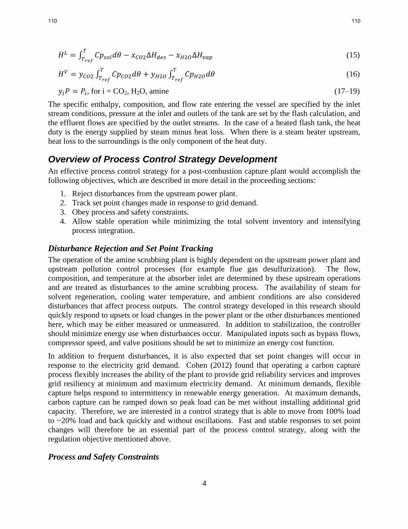
4

∫

(15)

∫

∫

(16)

, for i = CO2, H2O, amine (17–19)

The specific enthalpy, composition, and flow rate entering the vessel are specified by the inlet

stream conditions, pressure at the inlet and outlets of the tank are set by the flash calculation, and

the effluent flows are specified by the outlet streams. In the case of a heated flash tank, the heat

duty is the energy supplied by steam minus heat loss. When there is a steam heater upstream,

heat loss to the surroundings is the only component of the heat duty.

Overview of Process Control Strategy Development

An effective process control strategy for a post-combustion capture plant would accomplish the

following objectives, which are described in more detail in the proceeding sections:

1. Reject disturbances from the upstream power plant.

2. Track set point changes made in response to grid demand.

3. Obey process and safety constraints.

4. Allow stable operation while minimizing the total solvent inventory and intensifying

process integration.

Disturbance Rejection and Set Point Tracking

The operation of the amine scrubbing plant is highly dependent on the upstream power plant and

upstream pollution control processes (for example flue gas desulfurization). The flow,

composition, and temperature at the absorber inlet are determined by these upstream operations

and are treated as disturbances to the amine scrubbing process. The availability of steam for

solvent regeneration, cooling water temperature, and ambient conditions are also considered

disturbances that affect process outputs. The control strategy developed in this research should

quickly respond to upsets or load changes in the power plant or the other disturbances mentioned

here, which may be either measured or unmeasured. In addition to stabilization, the controller

should minimize energy use when disturbances occur. Manipulated inputs such as bypass flows,

compressor speed, and valve positions should be set to minimize an energy cost function.

In addition to frequent disturbances, it is also expected that set point changes will occur in

response to the electricity grid demand. Cohen (2012) found that operating a carbon capture

process flexibly increases the ability of the plant to provide grid reliability services and improves

grid resiliency at minimum and maximum electricity demand. At minimum demands, flexible

capture helps respond to intermittency in renewable energy generation. At maximum demands,

carbon capture can be ramped down so peak load can be met without installing additional grid

capacity. Therefore, we are interested in a control strategy that is able to move from 100% load

to ~20% load and back quickly and without oscillations. Fast and stable responses to set point

changes will therefore be an essential part of the process control strategy, along with the

regulation objective mentioned above.

Process and Safety Constraints

110 110

5

Varying degrees of constraints exist in the amine scrubbing process. Some constraints

correspond to hard input constraints that cannot physically be violated, for example the

maximum speed of the compressor or the maximum pressure of steam available from the IP/LP

crossover. Soft operational constraints, like the solvent degradation temperature, can be

temporarily violated but an appropriate control design would penalize these violations so the

process conditions quickly return to acceptable values. Finally, hard safety constraints like the

maximum pressure and temperature rating of a heat exchanger, the compressor surge limit, and

pressure limit for pump cavitation must be obeyed at all times because violating them could lead

to a plant shutdown and potentially create serious safety issues. These process constraints must

be taken into consideration for an effective control strategy design.

Multiple Time Scale Behavior

The general trend in the chemical process industry is the development of increasingly integrated

process designs that use extensive material and energy recycling and minimize overall inventory.

With enormous capital and operating costs, amine scrubbing will certainly adhere to this trend.

Figure 2 shows the material flows in a typical amine scrubbing process. Fis denotes the molar

flow of stream i at steady state. Based on the work of Baldea & Daoutidis (2012), the following

observations are made regarding the relative magnitudes of these flows:

i. The nominal flows of the amine solvent streams in the recycle loop, the CO2-rich solvent

flow (FRichs) and the CO2-lean solvent flow (FLean

s), are of comparable magnitude:

ii. The amount of CO2 entering the absorber in the flue gas (FCO2,ins) is of comparable

magnitude to the amount of CO2 exiting the stripper (FCO2,outs):

iii. The flow of the recycled solvent is much greater than the combined CO2 throughput and

the makeup amine and water (FAmines and FH2O

s), which is reflected in a large recycle

number (Rc):

iv. The flow of the purge stream is much smaller than the rate of material entering the

system, reflected in a small purge number (Pu):

These observations may suggest that the overall plant is a singularly perturbed system with the

possible existence of three distinct time scales: a fast time scale at the unit level associated with

the large recycle loop flows, an intermediate time scale at the process level associated with the

small feed and product flows, and a slow time scale of impurity levels associated with the purge

stream. A time scale decomposition will be performed to confirm whether the system is

singularly perturbed. Singularly perturbed systems complicate model-based process control

because the equations are inherently stiff and reduced order modeling is required.

In order to satisfy control objectives while simultaneously minimizing solvent inventory and

maximizing material and energy recycling, the controller design must take into account the

111 111

6

presence of multiple time scales. When systems are clearly separable into multiple time scales

such as amine scrubbing, a hierarchical control strategy is warranted (Scattolini, 2009). At the

fast unit-level time scale, standard PI controllers are usually sufficient to achieve regulatory

objectives such as level control. At the intermediate and slow time scales, a supervisory

controller is needed to achieve overall process objectives, such as the percentage of CO2

removed from the flue gas.

Figure 2: Process material and energy flows.

Literature Review of Amine Scrubbing Process Control

Limited examples exist of process control strategy development for amine scrubbing. Ziaii

(2012) developed a multi-loop cascade controller that showed adequate disturbance rejection and

set point tracking. Panahi & Skogestad (2011) used an economic optimization procedure to

select the best self-optimizing controlled variables. This work was extended (Panahi &

Skogestad, 2012) to include a plantwide control strategy consisting of a regulatory layer with

PID control and a supervisory layer with model predictive control. The dynamic model of the

plant used to test this control scheme contains significant simplifications and assumptions.

Åkesson et al. (2012) developed a nonlinear model predictive controller for the stripper and

demonstrated the controller on a simplified plant model.

Conclusions

A thermophysical properties library has been developed for piperazine which can be

called by any unit operation model developed in gPROMS®.

Including vapor hold-up may be important to accurately simulate transient behavior, and

the separator vessel model has been updated to include vapor hold-up in the overall

material inventory.

The main process control objectives for amine scrubbing are disturbance rejection, set

point tracking, satisfying constraints, and stable operation with process intensification.

Because of the significant material and energy recycle, amine scrubbing is expected to

exhibit multiple time scale behavior, suggesting the need for a hierarchical controller

design.

Future Work

Implement a model for a segment of stripper packing in gPROMS®.

112 112

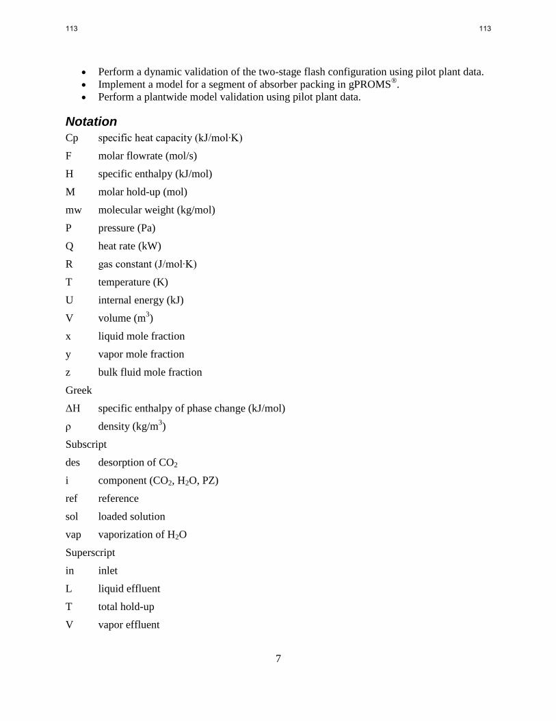
7

Perform a dynamic validation of the two-stage flash configuration using pilot plant data. Implement a model for a segment of absorber packing in gPROMS

®.

Perform a plantwide model validation using pilot plant data.

Notation

Cp specific heat capacity (kJ/mol∙K)

F molar flowrate (mol/s)

H specific enthalpy (kJ/mol)

M molar hold-up (mol)

mw molecular weight (kg/mol)

P pressure (Pa)

Q heat rate (kW)

R gas constant (J/mol∙K)

T temperature (K)

U internal energy (kJ)

V volume (m3)

x liquid mole fraction

y vapor mole fraction

z bulk fluid mole fraction

Greek

ΔH specific enthalpy of phase change (kJ/mol)

ρ density (kg/m3)

Subscript

des desorption of CO2

i component (CO2, H2O, PZ)

ref reference

sol loaded solution

vap vaporization of H2O

Superscript

in inlet

L liquid effluent

T total hold-up

V vapor effluent

113 113

8

References

Åkesson J, Laird CD, Lavedan G, Prölß K, Tummescheit H, Velut S, Zhu Y. " Nonlinear Model

Predictive Control of a CO2 Post-Combustion Absorption Unit." Chem Eng Tech.

2012:35(3);445–454.

Baldea M, Daoutidis P. Dynamics and Nonlinear Control of Integrated Process Systems. New

York, Cambridge University Press. 2012.

Cohen SM. A Techno-economic Plant- and Grid-Level Assessment of Flexible CO2 Capture. The

University of Texas at Austin. Ph.D. Dissertation. 2012.

Frailie PT, Plaza JP, Van Wagener DH, Rochelle GT. "Modeling piperazine thermodynamics."

Energy Proc. 2011;4:35–42.

Freeman SA. Thermal Degradation and Oxidation of Aqueous Piperazine for Carbon Dioxide Capture. The University of Texas at Austin. Ph.D. Dissertation. 2011.

Kvamsdal HM, Jakobsen JP, Hoff KA. "Dynamic Modeling and Simulation of a CO2 Absorber

for Post-Combustion CO2 Capture." Chemical Engineering and Processing: Process

Intensification. 2009:48(1);135–144.

Kumar A, Daoutidis P. "Modeling, analysis and control of ethylene glycol reactive distillation

column." AIChE J. 1999;45(1):51–68.

Lawal A, Wang M, Stephenson P, Yeung H. "Dynamic Modeling and Simulation of CO2

Chemical Absorption Process for Coal-Fired Power Plants." Computer Aided Chemical

Engineering. 2009:27;1725–1730.

Panahi M, Skogestad S. "Economically Efficient Operation of CO2 Capturing Process PartI:

Self-Optimizing Procedure for Selecting the best Controlled Variables." Chemical

Engineering and Processing: Process Intensification. 2011:50(3);247–253.

Panahi M, Skogestad S. "Economically Efficient Operation of CO2 Capturing Process. Part II.

Design of Control Layer." Chemical Engineering and Processing: Process Intensification.

2012:52;112–124.

Scattolini R. "Architectures for Distributed and Hierarchical Model Predictive Control- A

Review." J Proc Cont. 2009:19;723–731.

Tobieson FA, Hillestad M, Kvamsdal H, Chikukwa A. "A General Column Model in CO2SIM

for Transient Modelling of CO2 Absorption Processes." Energy Proc. 2012:23;129–139.

Walters MS, Dunia RH, Edgar TF, Rochelle GT. "Two-stage flash for CO2 regeneration:

dynamic modeling and pilot plant validation." In: 11th International Conference on

Greenhouse Gas Control Technologies. Kyoto, Japan. 2012.

Xu Q. Thermodynamics of CO2 Loaded Aqueous Amines. The University of Texas at Austin.

Ph.D. Dissertation. 2011.

Ziaii SF. Dynamic Modeling, Optimization, and Control of Monoethanolamine Scrubbing for

CO2 Capture. The University of Texas at Austin. Ph.D. Dissertation. 2012.

114 114

9

Appendix

In Visual Studio 2012®, the following steps should be taken to create a DLL containing the

thermophysical properties of an amine solvent:

1. File → New → Project.

2. Select Win32 Console Application, and change name/location as desired.

3. In the wizard, Next → Select DLL as application type and check empty project → Finish.

4. Right click Source Files → Add → Existing: Add your main .cxx file. This should be a

modified version of foi_demo_cpp.cxx which is provided by PSE. You only need to

change the equations and function names, the shell of the code should not be changed.

5. Right click Header Files → Add → Existing: Add foi_demo_cpp.h, gFOInterface.cxx,

and gFPClass.h (Program files → PSE → ModelBuilder_3.x → src → include & …→

src → foi → C++).

6. Project → Properties → C/C++ → General → Additional include directories → Edit:

Add any directory where #include files are located (same directories as step 5).

7. Still in Properties, go to Linker → General → Additional Library Directories → Edit:

Add the location of the gCommon Libarary (Program files → PSE → gPROMS-core_3.x

→ bin).

8. Still in Linker, go to Input → Additional Dependencies → Edit: Type gCommon.lib.

9. Go to Build → Build Solution. Copy the DLL file created into the appropriate directory

to run in gPROMS (Program files → PSE → ModelBuilder_3.x → fo will work).

You may need to change the platform in Visual Studio® from the Win32 (which is the default) to

x64 since gCommon.lib was compiled using a 64-bit machine:

1. Right click the solution at the top of the tree → Properties.

2. Select Configuration properties → Configuration Manager.

3. Active Solution Platform → New → Select x64 → OK.

4. Platform should now say x64.

By following these steps and using consistent notation, the properties of any nonvolatile amine

can be incorporated into the general amine scrubbing model being built in gPROMS®.

115 115

1

Effect of viscosity on liquid mass transfer coefficient


by Di Song




July 31, 2013

Abstract

The packed column plays a central role in industry separation processes. Packing is also

used for post combustion CO2 capture. Studies have been done on how the character of

liquid, gas, packing, column, and other auxiliary equipment can affect mass transfer

efficiency. It is important to know how liquid viscosity influences mass transfer efficiency

because the amine solvents used for CO2 scrubbing have significantly greater viscosity than

water. However, few models provide satisfactory prediction for viscous systems. The

inaccuracy results from the use of water only, limited equipment size, and improper

theoretical modeling. It is necessary to investigate the influence of viscosity on mass

transfer in packed columns.

In this quarter, the review of literature about liquid side mass transfer models was continued.

Particular attention has been paid to the effect of liquid viscosity alone together with its effect

on diffusivity on mass transfer in the liquid phase. A revised research plan is proposed to

see how liquid viscosity affects mass transfer by stripping toluene from water/glycerol.

Pulsed-field gradient nuclear magnetic resonance (PFG-NMR) has been chosen as a tool for

measuring the diffusion coefficient in the liquid side. Assistance was also provided with a

packing characterization experiment performed by Chao Wang at the Separations Research

Program (SRP). In the experiment, the hydraulic performance, effective mass transfer area,

and gas/liquid side mass transfer coefficient of the packing were measured.

Literature review

Models of liquid side mass transfer efficiency in packed columns

In the last quarterly report, a literature review of liquid side mass transfer coefficient models

has been done. Predictions of the dependence of kL on liquid viscosity disagree drastically

with each other, with the exponent varying from 0.53 to -0.103 (see Figure 1). This results

from the fact that most experiments use only an aqueous system which has insignificant

variance in viscosity. For the few correlations in which liquid viscosity was varied over a

wide range, either the column size is small, or only random packing was investigated.

116 116

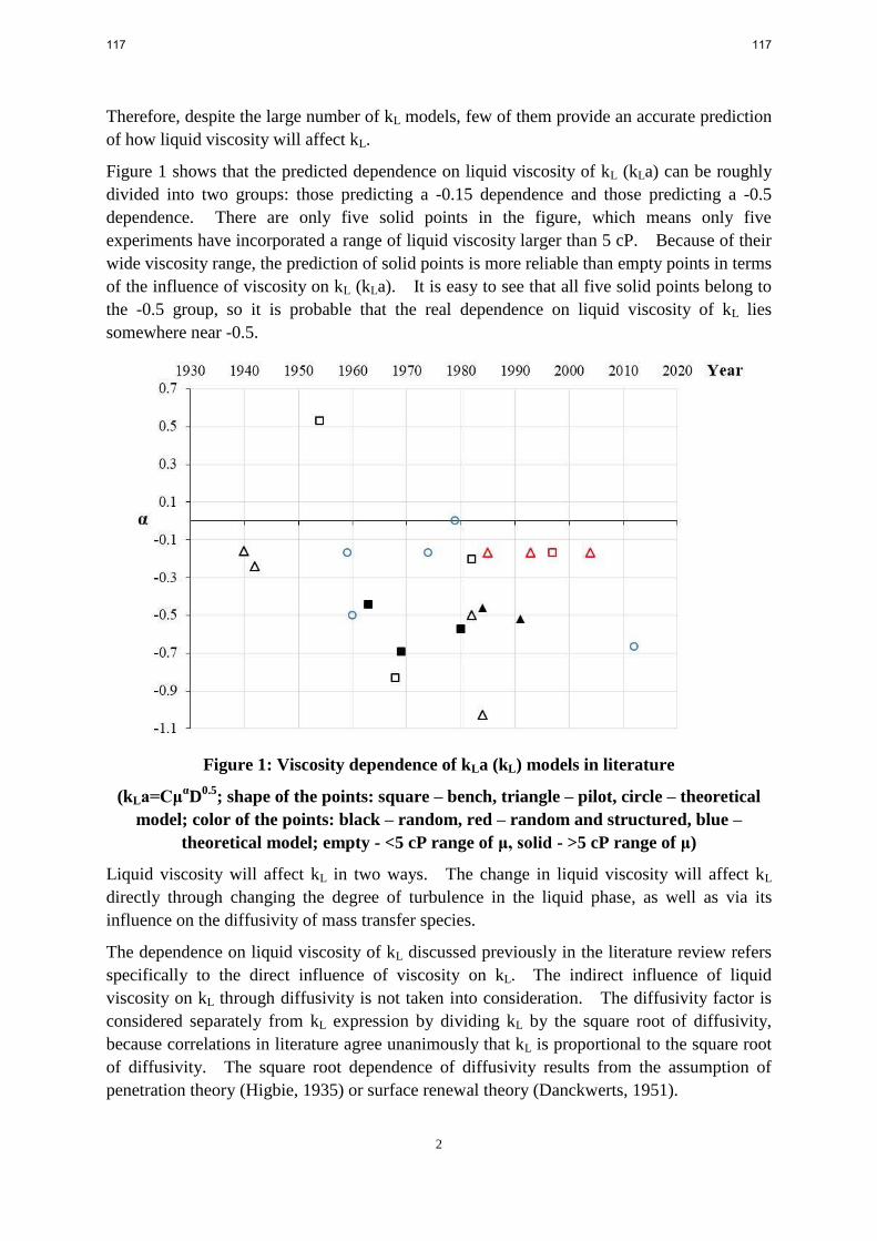
2

Therefore, despite the large number of kL models, few of them provide an accurate prediction

of how liquid viscosity will affect kL.

Figure 1 shows that the predicted dependence on liquid viscosity of kL (kLa) can be roughly

divided into two groups: those predicting a -0.15 dependence and those predicting a -0.5

dependence. There are only five solid points in the figure, which means only five

experiments have incorporated a range of liquid viscosity larger than 5 cP. Because of their

wide viscosity range, the prediction of solid points is more reliable than empty points in terms

of the influence of viscosity on kL (kLa). It is easy to see that all five solid points belong to

the -0.5 group, so it is probable that the real dependence on liquid viscosity of kL lies

somewhere near -0.5.

Figure 1: Viscosity dependence of kLa (kL) models in literature

(kLa=CμαD

0.5; shape of the points: square – bench, triangle – pilot, circle – theoretical

model; color of the points: black – random, red – random and structured, blue –

theoretical model; empty - <5 cP range of μ, solid - >5 cP range of μ)

Liquid viscosity will affect kL in two ways. The change in liquid viscosity will affect kL

directly through changing the degree of turbulence in the liquid phase, as well as via its

influence on the diffusivity of mass transfer species.

The dependence on liquid viscosity of kL discussed previously in the literature review refers

specifically to the direct influence of viscosity on kL. The indirect influence of liquid

viscosity on kL through diffusivity is not taken into consideration. The diffusivity factor is

considered separately from kL expression by dividing kL by the square root of diffusivity,

because correlations in literature agree unanimously that kL is proportional to the square root

of diffusivity. The square root dependence of diffusivity results from the assumption of

penetration theory (Higbie, 1935) or surface renewal theory (Danckwerts, 1951).

117 117

3

As the influence of liquid viscosity on kL will be investigated, the indirect influence of

viscosity through diffusion coefficient cannot be simply omitted or considered in isolation.

Therefore, the literature was reviewed to see how the diffusivity was measured and expressed

as a function of liquid viscosity in previous kL/kLa correlations.

The results of the review were disappointing. Much of the previous work did not vary the

viscosity or the diffusion coefficient (Molstad et al., 1942; Knoedler and Bonilla, 1954;

Shulman et al., 1955; Mohunta et al., 1969; Brunnazi and Paglianti. 1997; Murrieta et al.,

2004). As with viscosity, the effect of diffusivity is usually incorporated into the correlation

as a part of the dimensionless group to satisfy the form of penetration theory or surface

renewal theory (Davidson, 1959; Bridgwater and Scott, 1974; Ponter and Au-Yeung, 1982).

For correlations with variable liquid phase diffusion coefficients, the value of diffusivity is

either measured using the laminar jet method, calculated from other correlations, or extracted

from a data bank. Very few correlations have attempted to further investigate how liquid

viscosity affects the diffusion coefficient or to express diffusivity as a function of liquid

viscosity.

For correlations of Cornell et al. (1960), Bolles and Fair (1982), Bravo et al. (1985), and

Billet & Schultes (1999), the soundness of their semi-theoretical correlation was tested

through data from both their own experiments and previously published data of others.

Though diffusivity is varied in their data bank, the value is not measured in a systematic way

and how these values are acquired in each data source is not specified. Mangers and Ponter

(1980), and Xu et al. (2000) varied liquid phase diffusivity in their own experiments, but the

method for measurement is not specified. The diffusivity data of Sherwood and Holloway

(1940) were obtained from I.C.T. and were corrected to a standard temperature according to

the Stokes-Einstein equation. Norman and Sammak (1963) and Echarte et al. (1984)

measured the diffusion coefficient using laminar liquid jets. Delaloye et al. (1991)

calculated the diffusion coefficient based on a diffusivity correlation (Lohse et al., 1981).

Despite the difference in how their diffusivity data are acquired, none of the above kL/kLa

correlations has investigated the influence of liquid viscosity on liquid phase diffusivity. In

these correlations, diffusivity is regarded as an independent variable affecting kL, which is not

the case. The correlation of Onda et al. (1968) is the only one in the reviewed literature that

has taken into consideration the influence of liquid viscosity on diffusivity. The diffusivity

is considered to be proportional to viscosity to the -0.9 according to a modified

Stokes-Einstein equation.

Based on the results of the literature review, there is a need for an experiment that accurately

measures liquid phase diffusivity so that a correlation for diffusivity can be built to account

for the influence of liquid viscosity on diffusivity. Only in this way can we obtain the

complete influence of liquid viscosity on kL in both ways of directly affecting liquid

turbulence and indirectly affecting the diffusivity. Moreover, despite the fact that almost all

kL/kLa correlations predict the liquid side mass transfer coefficient to be proportional to the

square root of diffusivity, it is more reliable if the dependence on diffusivity of kL can be

correlated directly based on the empirical data instead of idealized theories like penetration

theory or surface renewal theory.

118 118

4

Correlations of diffusion coefficient

The objective of the proposed experiment is to investigate the complete influence of liquid

viscosity on kL. As is discussed before, the diffusivity is not an independent variable but a

function of physical properties including liquid viscosity. Therefore, it is necessary to find

out the proper correlation describing the diffusion coefficient as a function of liquid viscosity.

Based on the assumption that molecules are spherical in shape, the diffusion coefficient can

be described by the Stokes-Einstein equation (Einstein, 1905; Sutherland, 1905):

(1)

The Stokes-Einstein equation is a theoretical correlation. According to Equation 1,

diffusion coefficient is inversely proportional to liquid viscosity. The other parameters are

constant for a specific system if temperature is assumed to be constant. Equation 1

describes the diffusion coefficient in the ideal situation where all molecules are perfectly

spherical. Though in the real situation this is not necessarily the case, Equation 1 gives us

the idea that an increasing liquid viscosity will lead to a decrease in diffusion coefficient and

thus a further decrease in kL. The Stokes-Einstein has been widely used in its modified

forms derived from more rigorous assumptions.

The diffusivity correlation of Wilke and Chang (1955) is shown in Equation 2. The

correlation is based on a large database with numerous combinations of solutes and solvents.

The correlation is designed for dilute solutions. A more detailed investigation into the

solute-solvent interaction is needed if a higher accuracy of diffusivity is required.

( ) ⁄

(2)

Lohse et al. (1981) has developed a correlation, shown in Equation 3, to predict the diffusion

coefficient of CO2 in different diluted polymer solutions. This correlation investigates

specifically the influence of liquid viscosity on diffusivity and agrees with the assumption

that, for very long polymer chains (very large M value), the diffusion coefficient is not

significantly influenced by the viscosity of the solvent.

(

) √ ⁄

(3)

Though various correlations of diffusivity are available in literature, the most reliable and

accurate method to obtain diffusivity data is still the direct measurement of the system

incorporated in the mass transfer experiment. Therefore, the diffusivity will be measured

directly in this research and a new correlation of diffusivity will be developed based on the

empirical data. Prediction of the new diffusivity correlation will be compared with the

correlations in literature to check the soundness of the new correlation.

Measurements of diffusion coefficient

Extra caution should be exercised in choosing the measuring method of physical properties of

the tested system. Three methods are discussed here: laminar liquid jets, wetted wall

column, and pulsed-field gradient nuclear magnetic resonance (PFG-NMR).

Laminar liquid jets (Hogendoorn et al., 2002) have been used to measure the diffusivity of

slightly soluble gases in the gas-liquid mass transfer. The jet reactor consists of a

119 119

5

cylindrical tube through which the liquid flows into the gas. Gas is absorbed into the liquid

during the contact time. The liquid is then collected and the concentration measured. The

jets can be regarded as a liquid cylinder moving at constant velocity, so the effective mass

transfer area and contact time of the gas and liquid can be easily determined. The advantage

of the laminar liquid jet method is that a relatively wide range of contact time can be chosen.

Equation 4 is used to determine the diffusivity of certain chemical species in a liquid.

( )√ (4)

The wetted wall column (Hogendoorn et al., 2002) has the advantage of a known effective

mass transfer area because of the reactor geometry. It is widely used for mass transfer

experiments between gas and liquid. Based on the assumptions made about the mass

transfer pattern at the gas-liquid interface and correlations of mass transfer coefficient, and

the data of total mass transfer rate, the diffusion coefficient can be calculated.

The PFG-NMR method was first demonstrated by Stejskal and Tanner (1965). In this

method, a certain pulse sequence in a specific time period is added in a constant magnetic

field gradient. Due to the translational diffusion, the spin of particle will undergo a process

of “dephase” and thus lead to the attenuation of echo signals. The diffusion coefficient is

calculated based on how much the echo signal has decayed. The diffusivity can be

calculated from Equation 5 (Price, 1997). The advantage of PFG-NMR method is its

noninvasive nature and high resolution in data display.

[ ( ⁄ ) ] (5)

PFG-NMR is chosen because of its superior accuracy compared to the laminar liquid jet

method. The wetted wall column method is not chosen because it is based on some

important assumptions including the mass transfer correlation which are yet to be determined

in this research.

Experimental Work

In this quarter, a packing characterization experiment has been conducted under the

instruction of Chao Wang. The hydraulic and mass transfer performance of two structured

metal packings, GTC 500Y and Mellapack 2X, were tested. Liquid hold-up, column

pressure drop, effective mass transfer area, liquid side mass transfer coefficient, and gas side

mass transfer coefficient have been measured. The experimental approach is the same as

the previous experiments conducted by SRP (Wang et al., 2012).

Safety Issues

1. Safety helmets are required for experiments outside the control room.

2. Alkaline solvents (NaOH) should be neutralized to pH 6–10 before draining.

3. Gas mask with respirator is required when handling volatile and toxic chemicals.

4. Steel reinforced gloves are required when handling sheet metal structured packings.

120 120

6

Future Work & Experimental Plan

The objective of the upcoming experiment is to determine the dependence on liquid viscosity

of liquid side mass transfer coefficient. The experiment consists of two main parts. The

first part is the mass transfer experiment to be carried out in the pilot-scale absorber at the

Pickle Research Campus. A change has been made to the experimental plan described in

the last quarterly report: ae measurements will not be made, instead the area correlation of

Tsai (2010) will be used to calculate the effective mass transfer area. The change is made

mainly for economic reasons. The second part is the PFG-NMR experiment to determine

the value of diffusion coefficient of toluene in water/glycerol and water/PEG. The empirical

data will be used to predict diffusivity as a function of liquid viscosity.

Experimental concerns

The intensity of the NMR signal of toluene might be too low to be observed. If this is the

case, the diffusion coefficient of benzene will be measured as a substitute for toluene because

the signal intensity of benzene will be much higher than that of toluene due to the sameness

and symmetry of carbon atoms in the molecule of benzene. Benzene is chosen as

prospective substitute because its molecular structure is similar to toluene.

Conclusions

1. kL/kLa correlations in the literature agree unanimously that the liquid side mass transfer

coefficient is proportional to the square root of diffusivity.

2. Few kL/kLa correlations in the literature have discussed the indirect influence of viscosity

on the liquid side mass transfer coefficient via diffusivity.

3. For the direct influence of viscosity on kL/kLa, correlations in literature can be divided

into two groups: those predicting a -0.15 dependence and those predicting a -0.5

dependence. The predictions of the latter group are more reliable.

Nomenclature

ae = effective area of packing, m2/m

3

ap = specific area of packing, m2/m

3

D = diffusivity, m2/s

D0 = diffusivity of CO2 in water, m2/s

g = gradient of magnetic field, T/m

I = intensity of NMR signal

LJ = length of liquid jets, m

L = liquid flow rate, m3/s

M = molecular weight of solvent

M0 = molecular weight of water

R = ideal gas constant, (m3-Pa)/(kmol-K)

r = rate of gas absorption, mol/s

Re = Reynolds number, uρd/μ

121 121

7

Sc = Schmidt number, μ/ρD

T = absolute temperature, K

uG = gas velocity, m/s

uL = liquid velocity, m/s

V = molar volume of solute at normal boiling point, cc/(g-mol)

= association parameter, multiple of nominal molecular weight of solvents

= time between two gradient pulses, s

= duration of gradient pulse, s

μ = viscosity, cP

σ = surface tension, dyn/cm

θ = contact angle, deg

References

Billet R, Schultes M. "Prediction of mass transfer columns with dumped and arranged

packings – updated summary of the calculation method of Billet and Schultes." Chem

Eng Res Des. 1999;77(6):498–04.

Bolles WL, Fair JR. "Improved mass-transfer model enhances packed-column design." Chem

Eng. 1982;89(14):109–116.

Bravo LJ, Rocha JA, Fair JR. "Mass transfer in gauze packings." Hydroc Proc.

1985;64(1):91–95.

Bridgwater J, Scott AM. "Statistical models of packing. Application to gas absorption and

solids mixing." Trans Inst Chem Eng. 1974;52(4):717–324.

Brunazzi E, Paglianti A. "Liquid-film mass-transfer coefficient in a column equipped with

structured packings." Ind Eng Chem Res. 1997;36(9):3792–3799.

Cornell ID, Knapp WG, Fair JR. "Mass-transfer efficiency. Packed columns." ChemEng Prog.

1960;56(7):68–74.

Danckwerts PV. "Significance of liquid-film coefficients in gas absorption." Ind Eng Chem.

1951;43(6):1460–1467.

Davidson JF, IMech.E AM. "The hold-up and liquid film coefficient of packed towers Part 2:

statistical models of the random packing." Trans Inst Chem Eng. 1959;37(1):131–136.

Delaloye MM, von Stockar U,Lu XP. "The influence of viscosity on the liquid phase mass

transfer resistance in packed columns." Chem Eng J. 1991;47(1):51–61.

Echarte R, Campana H, Brignole EA. "Effective area and liquid film mass transfer coefficient

in packed columns." Industrial and engineering chemistry process design and

development. 1984;23(2):349–354.

Einstein A. “On the movement of small particles suspended in stationary liquids required by

the molecular-kinetic theory of heat.” Annalen der Physik. 1905;17(8):549–560.

Higbie R. "The rate of absorption of a pure gas into a still liquid during short periods of

exposure." Trans Am Inst Chem Eng. 1935;31:365–389.

Hogendoorn JA, Vas Bhat RD, Versteeg GF. “On the Determination of the Diffusivity of CO2

122 122

8

in Aqueous and NonAqueous Solvents: Investigations with Laminar Jets and Wetted

Wall Columns.” ChemEng Comm. 2002;189(8):1009–1037.

Knoedler EL, Bonilla CF. "Vacuum degasification in a packed column. Deoxygenation of

water in Stedman packing" Chem Eng Prog. 1954;50(1):125–133.

Lohse M, Alper E, Quicker G, Deckwer WD. “Diffusivity and solubility of carbondioxide in

diluted polymer solutions.” AIChE J. 1981;27(4):626–631.

Mangers RJ, Ponter AB. "Effect of Viscosity on Liquid Film Resistance to Mass Transfer in a

packed column."Ind Eng Chem Process Des Dev . 1980;19(4):530–537. DOI:

10.1021/i260076a005.

Mohunta DM, Vaidyanathan AS, Laddha GS. "Prediction of liquid-phase mass transfer

coefficients in columns packed with Raschig rings" Indian Chem Eng. 1969;11(3):73–79.

Murrieta CR, Seibert AF, Fair JR, Rocha JA. "Liquid-side mass-transfer resistance of

structured packings." IECR. 2004;43(22):7113–7120.

Norman WS, Sammak FYY. "Gas absorption in a packed column Part 1: the effect of liquid

viscosity on the mass transfer coefficient." Trans Inst Chem Eng. 1963;41(3):109–116.

Onda K, Takeuchi H, Okumoto Y. "Mass transfer coefficients between gas and liquid phases

in packed columns." J Chem Eng Jpn. 1968;1(1):56–62.

Ponter AB, Au-Yeung PH. "Estimation of liquid film mass transfer coefficients in columns

packed randomly with partially wetted rings." Can J ChemEng. 1982;60(1):94–99.

Price WS. “Pulsed-field gradient nuclear magnetic resonance as a tool for studying

translational diffusion: part 1 Basic theory.” Magn Res: Educ J. 1997;9(5):299–336.

Shulman HL, Ullrich CF, Proulx AZ, Zimmerman JO. "Performance of packed columns. II.

Wetted and effective-interfacial areas, gas - and liquid-phase mass transfer rates." AIChE

J. 1955;1(2):253–258.

Stejskal EO, Tanner JE. “Spin Diffusion Measurements: Spin Echoes in the Presence of a

Time-dependent field gradient.” J Chem Phys. 1965;42(1):288–292.

Sutherland W. “A dynamical theory of diffusion for non-electrolytes and the molecular mass

of albumin.” Philos Mag. 1905;9(54):781-785.

Tsai RE. Mass Transfer Area of Structured Packing. The University of Texas at Austin. Ph.D.

Dissertation. 2010.

Wang C, Perry M, Rochelle GT, Seibert AF. "Packing Characterization: Mass Transfer

Properties." Energy Proc. 2012a;23:23–32.

Wang C, Perry M, Seibert AF, Rochelle GT. "Characterization of novel structured packings

for CO2 Capture." GHGT-11, Kyoto, 2012.

Wilke CR, Chang P. “Correlation of diffusion coefficient in dilute solutions.” AICHE J.

1955;1(2):264–270.

Xu ZP, Afacan A, Chuang KT. "Predicting mass transfer in packed columns containing

structured packings." Chem Engin Res Des. 2000;78(A1):91–98.

123 123

1

Thermal Degradation of Activated Tertiary Amine Blends for Carbon Capture from Coal Combustion and Gas Treating


by Omkar Namjoshi




July 31, 2013

Abstract

The thermal degradation of activated tertiary amine solvents, including triethanolamine (TEA),

dimethylaminoethanol (DMAE), methyldiethanolamine (MDEA), diethylaminoethanol (DEAE),

and dimethylaminopropanol (DMAP) activated by piperazine (PZ) has been studied this quarter.

The solvent composition for each amine system is as follows: 7 m tertiary amine/2 m activator

with initial loadings of approximately 0.1 mol CO2/mol alkalinity and 0.25 mol CO2/mol

alkalinity. Degradation was studied at 150 oC and 135

oC. Loss of solvent alkalinity over time

was also studied for PZ-activated DMAP, MDEA, DMAE, DEAE, and

dimethylaminoethoxyethanol (DMAEE) solvents at 150 oC. Additionally, the ratio of

diethanolamine (DEA) and methylaminoethanol (MAE) present in degraded 5 m PZ/5 m MDEA

at 150 oC and an initial loading of 0.225 mol CO2/mol alkalinity was quantified using a new

cation chromatography method.





mmol/kg/h), and TEA (1.21 mmol/kg/h). The activation energy for thermal degradation for the

tertiary amines is as follows: DMAP (137 kJ/mol), DMAE (124 kJ/mol), MDEA (144 kJ/mol),

DEAE (172 kJ/mol), and TEA (123 kJ/mol). PZ degradation linear loss rates at these conditions

are similar to the tertiary amine loss rates in PZ-activated DMAP, DEAE, and TEA. The PZ loss

rate is substantially higher than the tertiary amine loss rate for PZ-activated MDEA and DMAE

blends.





mmol/kg/h), and TEA (1.21 mmol/kg/h). The PZ loss rate is substantially higher than the

tertiary amine loss rate in all PZ-activated tertiary blends with the exception of PZ-activated

DMAP.

124 124

2


Samples were prepared gravimetrically. CO2 was sparged into the solution and measured

gravimetrically. Approximately 4 ml of loaded amine solution was placed in 3/8” Swagelok®

stainless steel cylinders with a 4.5 ml capacity. These cylinders were sealed and placed in forced

convection ovens at set temperatures and removed periodically for analysis. Cation

chromatography (Dionex ICS-2100) was used to analyze for parent amine concentrations and

degradation by-product concentrations; samples were diluted by a factor of 10000, and the

separation was carried out using a Dionex CS17 column. Alkalinity was measured using a

Metrohm Titrando 835 autotitrator using 0.2 N sulfuric acid as the titrant; samples were diluted

by a factor of 300–600, and the amount of acid added to reach a pH of roughly 4 was used to

determine sample alkalinity. These methods are described in previous quarterly reports and

dissertations (Freeman, 2011) and will not be described in detail here.

New method development for separation of diethanolamine and methylaminoethanol

A new method was developed to separate diethanolamine (DEA) and methylaminoethanol

(MAE), two secondary amines present in the thermal degradation of PZ-activated MDEA

solvents. The existing cation chromatography method cannot separate these two compounds.

The new method uses a 4x50 mm CG19 Dionex guard column and a 4x250 mm CS19 Dionex

analytical column. Deionized water with a conductivity of 18.2 umho is used as the mobile

phase. A Dionex EGC II MSA eluent generation cartridge is used to provide either a gradient or

isocratic methylsulfonic acid concentration in the mobile phase. Samples are diluted by a factor

of 10000 to give a total amine concentration from 50 to 100 ppmw. Eluent flow is set to 0.4

ml/min to maintain a pressure just above 2000 psig at the pump head; this pressure is required to

properly degas the eluent cartridge. A CSRS 300 suppressor is used. Two sequential program

steps are used in this method.

In the first step, 25 µl of the diluted sample is injected into the column. A suppressor current of

5 mA is applied and the eluent concentration is held constant at 1 mM. This step lasts for 90

minutes and can resolve DEA and MAE. Bulkier monoamines, such as diethylaminoethanol

(DEAE) and polyvalent amines, such as PZ, are still bound to the column after the first step

ends; they cannot be removed due to the low eluent concentration used in the first step. Figure 1

is a representative chromatogram showing the separation of DEA and MAE.

125 125

3

Figure 1: Representative chromatogram of the new cation method that can separate

diethanolamine (DEA) and methylaminoethanol (MAE). The elution time for DEA is 57.2

minutes whereas the elution time of MAE is 59.5 minutes. MDEA is the large peak whose

elution time is approximately 75 minutes.

In the second program step, 25 µl of deionized water is injected into the column. A suppressor

current of 35 mA is applied and the eluent concentration is raised to 40 mM and held for 45

minutes. The increased eluent concentration allows for separation of the bulkier monoamines

and polyvalent amines that are still bound to the column. After 45 minutes, the eluent

concentration is reduced to 1 mM and held for 12.5 minutes to allow the column to equilibrate

prior to injection of the second sample. This step is also used for column equilibration prior to

running a sequence of samples. Figure 2 is a representative chromatogram showing the

separation of the polyvalent amines.

126 126

4

Figure 2: Representative chromatogram of the new cation method that can separate

diethanolamine (DEA) and methylaminoethanol (MAE) for the second injection.

Polyvalent amines, such as PZ and 1-methylpiperzine (1MPZ), have elution times of

approximately 9 and 11 minutes, respectively. Larger polyvalent amines, such as

triamines, tetramines, and pentamines, have elution times ranging from 15–20 minutes.

All amine solvents were prepared with identical starting concentrations: 7 m tertiary amine/2 m

activator with either an initial CO2 loading of 0.1 mol CO2/mol alkalinity or 0.25 mol CO2/mol

alkalinity.

Amines tested in this quarter include triethanolamine (TEA), dimethylaminoethanol (DMAE),

diethylaminoethanol (DEAE), dimethylaminopropanol (DMAP), methyldiethanolamine

(MDEA), and dimethylaminoethoxyethanol (DMAEE). Structures of these amines are presented

in Table 1.

127 127

5

Table 1: List of amines (names, abbreviated names, structures) tested this quarter

Amine Name Abbreviation Structure Role

Piperazine PZ

Activator

Triethanolamine TEA

Tertiary Amine

Methyldiethanolamine MDEA

Tertiary Amine

Dimethylaminoethanol DMAE

Tertiary Amine

Diethylaminoethanol DEAE

Tertiary Amine

Dimethylaminopropanol DMAP

Tertiary Amine

Dimethylaminoethoxyethanol DMAEE

Tertiary Amine

Safety

Representatives from ExxonMobil Chemical held a meeting with the department’s safety

committee and lab safety representatives to discuss how the chemical engineering department

can improve its safety culture on June 21, 2013. A recurring theme from the session indicated

that lab PIs, rather than the lab safety representative, should take leadership of all aspects of lab

safety. The results from the meeting will be shared with the department faculty at the next

advisory board meeting or at a faculty meeting.

Results

Amine losses were estimated using a pseudo-0th

order rate law, giving a linear rate loss

measurement in units of mmol/kg. The pseudo-0th

order rate law was used to understand the

relationship between the tertiary amine loss rate and the PZ loss rate as well as to understand the

degree of autocatalytic effects seen in the degradation of PZ-activated tertiary amines with at

least one hydroxyethyl group present. Table 2 summarizes the rate data and activation energies

NH NH

NOH

OH

OH

CH3N

OHOH

CH3N

CH3 OH

NOH

CH3

CH3

CH3N

CH3OH

CH3N

CH3 OOH

128 128

6

for experiments at an initial loading of 0.1 mol CO2/mol alkalinity and at an initial concentration

of 7 m PZ/2 m tertiary amine.

Table 2: List of initial thermal degradation rates of the tertiary amines activated by PZ

Conditions: 7 m tertiary amine/2 m PZ, initial loading 0.1 mol CO2/mol alk

Tertiary

Amine

Initial

Tertiary

Amine Loss,

mmol/h

Initial PZ

Loss, mmol/h

Activation Energy,

Tertiary Amine

(kJ/mol)

Activation Energy,

Piperazine

(kJ/mol)

TEA 135 oC: 0.21

150 oC: 1.2

175 oC: 5.8

135 oC: 0.17

150 oC: 1.2

175 oC: 8.7

124

147

MDEA 135 oC: 0.32

150 oC: 1.3

175 oC: 14.1

135 oC: 0.63

150 oC: 2.3

175 oC: 17.2

144

126

DMAE 135 oC: 0.71

150 oC: 2.39

175 oC: 23.9

135 oC: 0.88

150 oC: 3.3

175 oC: 23.2

124

134

DEAE 135 oC: 0.17

150 oC: 1.1

175 oC: 15.9

135 oC: 0.16

150 oC: 1.3

175 oC: 17.4

172

177

DMAP 135 oC: 0.36

150 oC: 1.6

175 oC: 13.3

135 oC: 0.34

150 oC: 1.6

175 oC: 11.0

137

131

Thermal degradation rates were also measured for PZ-activated TEA, MDEA, DMAE, DEAE,

and DMAP at an initial concentration of 7 m tertiary amine/2 m PZ, 150 oC, and an initial

loading of 0.25 mol CO2/mol alkalinity. The data from these experiments are summarized in

Table 3.

129 129

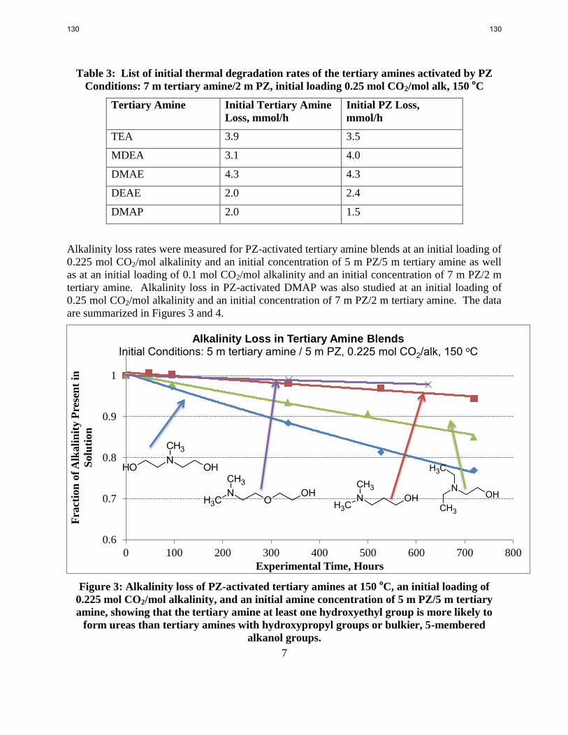
7

Table 3: List of initial thermal degradation rates of the tertiary amines activated by PZ

Conditions: 7 m tertiary amine/2 m PZ, initial loading 0.25 mol CO2/mol alk, 150 oC

Tertiary Amine Initial Tertiary Amine

Loss, mmol/h

Initial PZ Loss,

mmol/h

TEA 3.9 3.5

MDEA 3.1 4.0

DMAE 4.3 4.3

DEAE 2.0 2.4

DMAP 2.0 1.5

Alkalinity loss rates were measured for PZ-activated tertiary amine blends at an initial loading of

0.225 mol CO2/mol alkalinity and an initial concentration of 5 m PZ/5 m tertiary amine as well

as at an initial loading of 0.1 mol CO2/mol alkalinity and an initial concentration of 7 m PZ/2 m

tertiary amine. Alkalinity loss in PZ-activated DMAP was also studied at an initial loading of

0.25 mol CO2/mol alkalinity and an initial concentration of 7 m PZ/2 m tertiary amine. The data

are summarized in Figures 3 and 4.

Figure 3: Alkalinity loss of PZ-activated tertiary amines at 150 oC, an initial loading of

0.225 mol CO2/mol alkalinity, and an initial amine concentration of 5 m PZ/5 m tertiary

amine, showing that the tertiary amine at least one hydroxyethyl group is more likely to

form ureas than tertiary amines with hydroxypropyl groups or bulkier, 5-membered

alkanol groups.

0.6

0.7

0.8

0.9

1

0 100 200 300 400 500 600 700 800

Fra

ctio

n o

f A

lkali

nit

y P

rese

nt

in

Solu

tion

Experimental Time, Hours

Alkalinity Loss in Tertiary Amine Blends Initial Conditions: 5 m tertiary amine / 5 m PZ, 0.225 mol CO2/alk, 150 oC

CH3N

CH3 OOH

CH3N

OHOH

CH3N

CH3OH

NOH

CH3

CH3

130 130

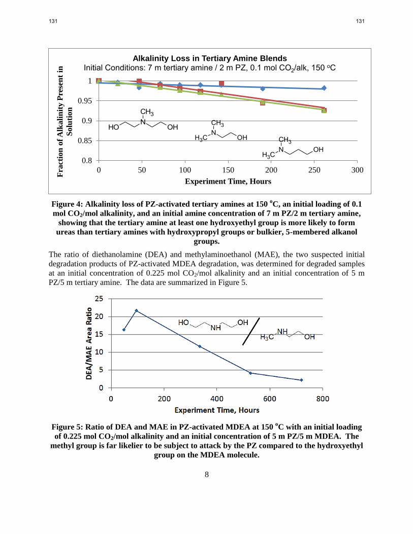
8

Figure 4: Alkalinity loss of PZ-activated tertiary amines at 150 oC, an initial loading of 0.1

mol CO2/mol alkalinity, and an initial amine concentration of 7 m PZ/2 m tertiary amine,

showing that the tertiary amine at least one hydroxyethyl group is more likely to form

ureas than tertiary amines with hydroxypropyl groups or bulkier, 5-membered alkanol

groups.

The ratio of diethanolamine (DEA) and methylaminoethanol (MAE), the two suspected initial

degradation products of PZ-activated MDEA degradation, was determined for degraded samples

at an initial concentration of 0.225 mol CO2/mol alkalinity and an initial concentration of 5 m

PZ/5 m tertiary amine. The data are summarized in Figure 5.

Figure 5: Ratio of DEA and MAE in PZ-activated MDEA at 150 oC with an initial loading

of 0.225 mol CO2/mol alkalinity and an initial concentration of 5 m PZ/5 m MDEA. The

methyl group is far likelier to be subject to attack by the PZ compared to the hydroxyethyl

group on the MDEA molecule.

0.8

0.85

0.9

0.95

1

0 50 100 150 200 250 300

Fra

ctio

n o

f A

lka

lin

ity P

rese

nt

in

Solu

tion

Experiment Time, Hours

Alkalinity Loss in Tertiary Amine Blends Initial Conditions: 7 m tertiary amine / 2 m PZ, 0.1 mol CO2/alk, 150 oC

CH3N

OHOH

CH3N

CH3OH

CH3N

CH3 OH

131 131

9

Analysis

Role of methyl, ethyl, and hydroxyethyl groups on initial degradation rate

Data strongly suggest that methyl groups are preferentially attacked over other substituent

groups. This is evident in the 95% selectivity of DEA, which is produced by PZ attacking the

methyl group on protonated MDEA, as opposed to MAE, which is produced by PZ attacking the

hydroxyethyl group on MAE, in PZ-activated MDEA solvents. At lower temperatures, where

the effects of autocatalysis and other degradation mechanisms might not be as strong, tertiary

amines with methyl substituent groups have the highest degradation rate. Tertiary amines

containing methyl groups also have the lowest activation energy compared to

diethylaminoethanol, which has no methyl groups present. The low activation energy seen for

PZ-activated TEA is not consistent with the data taken with an initial loading of 0.225 mol

CO2/mol alkalinity and initial concentration of 5 m PZ/5 m TEA. Regressing the activation

energy without the 175 oC data for the 7 m TEA/2 m PZ blend gives values of 187 kJ/mol for PZ

and 167 kJ/mol for TEA, which is in line with activation energies with data taken at an initial

concentration of 5 m PZ/5 m TEA and about a 30% upward deviation from the activation energy

values obtained by regressing the data for the entire temperature range. The activation energies

of the other activated tertiary blends showed deviations from -10% to +15% after removing the

data point at 175 oC.

Role of substituent groups on activator loss

This has been discussed in detail in a previous quarterly report (Rochelle, 2013) and will not be

repeated here. Trends seen in this set of experiments mirror those of experiments conducted with

an initial loading of 0.225 mol CO2/mol alkalinity and initial amine concentration of 5 m PZ/5 m

tertiary amine.

Role of hydroxyethyl and hydroxypropyl groups on alkalinity loss

The presence of hydroxyethyl groups can lead to higher alkalinity loss in the solvent. A

suspected pathway from an oxazolidinone to a cyclic urea is presented in Figure 6:

N

O

OR

1 + NH

OH

R2N

R2

OH

NH

R1

+O

O

N

R2

OH

NH

R1

SN2 Attack of R2 or OH

NHR3

NHR

1

132 132

10

Figure 6: Proposed pathway of cyclic urea formation starting from an oxazolidinone

intermediate from a tertiary amine with at least one hydroxyethyl group present.

In this reaction scheme, an oxazolidinone, which is formed from the secondary amine initial

degradation product from a tertiary amine with at least one hydroxyethyl group, can react with

the secondary amine degradation product to form a diamine. The diamine can then form a cyclic

urea. As shown in Figures 3 and 4, the tertiary amines with at least one hydroxyethyl group had

a greater rate of alkalinity loss compared to the amines without a hydroxyethyl group.

DMAP, which contains one hydroxypropyl group, forms a six-membered oxazolidinone instead

of a five-membered oxazolidinone. The six-membered heterocycle is presumed to be

significantly harder to form than the five-membered heterocycle as evidenced by the

accumulation of methylaminopropanol in degraded PZ-activated samples (Rochelle, 2013) and

an alkalinity loss of roughly 2%/wk. DMAEE, which cannot form an oxazolidinone, has a much

reduced alkalinity loss rate compared to DMAP. Solutions containing PZ-activated DMAP or

PZ-activated DMAEE are presumed to go through another alkalinity loss pathway that does not

involve the hydroxyl functional group.

Role of pKa and increased CO2 loading on initial degradation rate

Increasing the CO2 loading had a stronger effect on the loss of tertiary amine compared to the

activator, although the increase in degradation rate varied from as little as 20% for DMAP to

more than 200% for TEA. The differences in the magnitude of the degradation rate could be

dependent on pKa: TEA, with a low pKa, will have a relatively higher concentration of

protonated tertiary amine from a lower loading to a higher loading compared to tertiary amines

with high pKa values. An increased concentration of protonated tertiary amine, which is

susceptible to attack during the initial degradation step, would increase tertiary amine loss given

that the protonated tertiary amine is one of the species in the initial degradation step. On the

other hand, an increased concentration in protonated and/or carbamated PZ would reduce the PZ

loss rate because the initial degradation mechanism relies on a free amino group to attack a

protonated tertiary amine. On average, the tertiary amine loss at a loading of 0.25 mol CO2/mol

alkalinity increased by a factor of 2 whereas the PZ amine loss increased by a factor of 1.7

compared to the amine losses observed at a loading of 0.1 mol CO2/mol alkalinity.

DMAP losses were not significantly different at a higher loading than at a lower loading. The

intermediate product in DMAP, methylaminopropanol (MAP), is stable and has been observed to

NHR

3

NHR

1

Rxn with CO2 (Aq)

NHR

3

NR

1

O O-

NHR3

NR1

O O-N

R3

N R1

O

+ OH -

133 133

11

accumulate in degraded samples over time. It is possible that MAP could be in equilibrium with

the DMAP given that the DMAP can degrade to MAP and MAP can acquire a methyl group

(from protonated DMAP) to form free DMAP. Likewise, 1-methylpiperazine (1MPZ), the initial

degradation product between PZ and DMAP, could exchange a methyl group with MAP to form

DMAP and PZ and thus start to approach an equilibrium.

Conclusions

1. At 150 oC and an initial concentration of 7 m tertiary amine/2 m PZ and CO2 loading of

0.1, initial rates of thermal degradation and activation energy for the tertiary amines are:

TEA (1.2 mmol/h, 124 kJ/mol), MDEA (1.3 mmol/h 144 kJ/mol), DMAE (2.4 mmol/h

134 kJ/mol), DEAE (1.1 mmol/h 172 kJ/mol), DMAP (1.6 mmol/h 137 kJ/mol).

2. At 150 oC and an initial concentration of 7 m tertiary amine/2 m PZ and CO2 loading of

0.1, initial rates of thermal degradation and activation energy for PZ are: TEA (1.2

mmol/h, 147 kJ/mol), MDEA (2.3 mmol/h, 126 kJ/mol), DMAE (3.3 mmol/h, 124

kJ/mol), DEAE (1.3 mmol/h, 177 kJ/), DMAP (1.6 mmol/h, 131 kJ/mol).

3. Increased CO2 loading results in an increased rate of degradation of the tertiary amine

compared to piperazine in PZ-activated tertiary amine solvents.

4. PZ-activated tertiary amine solvents whose tertiary amine has at least one hydroxyethyl

group present lose alkalinity more rapidly than PZ-activated tertiary amine solvents

whose tertiary amine has no hydroxyethyl groups present.

5. The selectivity of DEA over MAE in the degradation of PZ-activated MDEA is greater

than 95%.

References

Freeman SA. Thermal Degradation and Oxidation of Aqueous Piperazine for Carbon Dioxide

Capture. The University of Texas at Austin. Ph.D. Dissertation. 2011.



134 134

1

Aerosol and Volatile Control in CO2 Capture


by Steven Fulk




July 31, 2013

Abstract

A modular Phase Doppler Interferometer (PDI) analyzer was tested at the Post-Combustion

Carbon Capture Center (PC4) on the Pilot Solvent Test Unit (PSTU) at the National Carbon

Capture Center (NCCC) in Wilsonville, Alabama on June 5, 2013. Equipment and technical

support of the analyzer was provided by William Bachalo and Chad Sipperley from Artium

Technologies, Inc. Southern Research Institute (SRI) provided optical access windows, set 140° apart, immediately downstream of the water wash column and a wooden support table for

particle measurement. Carl Landham of SRI coordinated and oversaw the demonstration.

A small, pocket-sized nebulizer was used to demonstrate the efficacy of the transmitter/receiver

system with ad hoc beam expander for a dense particle cloud containing 0.1–20 μm droplets.

The PDI analyzer measured a well-behaved, log-mean particle distribution with a count-mean

diameter of around 5 μm.

The analyzer was then set in place and realigned to measure the droplet size distribution at the

center of the duct exiting the water wash. The PDI analyzer was unable to measure a particle

size distribution due to the high concentration of particles ≤ 1 μm. Though larger particles were

visually present, the dense fog of submicron drops precluded a measureable response above the

background signal.

Artium has suggested that focusing the transmitted lasers to 2–5 μm in diameter (50 μm was

used in this test) would increase signal response at higher particle concentrations; however, the

optical path length will need to be reduced. The Self-Contained PDI system used on the aerosol

growth column would provide ideal conditions for measurement.

The high concentration of submicron particles indicates that coagulation is likely still an

important mechanism for aerosol growth/agglomeration. Furthermore, the contribution of the

aerosol mass to the total mass balance is significant and must be accounted for in simulations.

Particle growth may be inhibited by gas-side mass transfer of amine from the bulk solvent.

Fabrication of the aerosol growth column continued in this quarter. The absorber column, sump,

distributor inlets, and the presaturator vessel have been sent off for fabrication and welding. The

extruded aluminum structural framing and support plates for flanged elements were fabricated

and bolted in place. Power supplies and control/measurement device connections have been

135 135

2

wired. Liquid and gas tubing have been cut and swaged in place where allowable without the

welded pieces for dimensioning.

Introduction

Volatile emissions are a primary concern for CO2 capture plants using amine scrubbers.

Emissions constitute increased economic expense through solvent loss as well as being a source

of potentially hazardous environmental pollutants. Compounds found in treated flue gas include

contaminants from thermal degradation and oxidation as well as combustion byproducts.

Degradation and reaction products have a wide range of toxicity and biodegradation

characteristics which potentially represent unacceptable emissions; as a result, recent work has

focused on estimating volatile losses and assessing their toxicological impact.

Volatile emissions can be reduced through the use of an absorber column using recycled water as

a solvent, called a water wash. Design considerations for water wash systems include liquid

distribution methods to adequately wet packing with small liquid rates, and balancing water in

the absorber/stripper system by adjusting the total volatile concentration in the wash water.

Water wash columns have relatively flat efficiency profiles, meaning the removal efficiency is

not a strong function of either the gas or liquid flow rates or the operating temperature.

Emissions with Aerosols

Recent pilot-plant measurements have shown that normal water wash columns are ineffective at

controlling volatile loss of amine and other pollutants due to the presence of aerosols. In 2011,

MHI presented pilot test results for both KS-1TM

and MEA which showed that emissions were

proportional to inlet SO3 concentration (MHI, 2012). Amine levels out of the wash section were

0.4–23.2 ppmv and 0.8–67.5 ppmv for KS-1TM

and MEA, respectively, for 0–3 ppmv inlet SO3.

Aerosols were visually present at the direct-contact cooler (DCC) and wash outlets. At the

Maasvlakte pilot plant, TNO and SINTEF jointly tested a 30 wt % MEA CO2 capture unit with a

downstream water wash complete with online gas and aerosol phase sampling (TNO, 2012;

SINTEF, 2012). Excessive emissions were observed; aerosols, not physical entrainment, were

responsible for the increase. Lithium and rubidium carbonate (Li2CO3, Rb2CO3) tracers in the

solvent and wash loops verified negligible entrainment. A Brownian demister unit (BDU) was

installed downstream of the wash section which reduced emissions to previously simulated

levels, indicating the bulk of emissions were contained in the droplet phase. Mean droplet

diameters (dDrop) were measured using light extinction coefficients and ranged between 0.76–

7.88 μm at the BDU inlet and 0.2–1.74 μm at the outlet. The quality of the inlet flue gas and the

absolute temperature of the absorber influenced the emission rate. More recently, a baseline

study using MEA at NCCC in Wilsonville, Alabama saw higher amine emissions than expected

(NCCC, 2012). The number of absorber beds (2–3), intercoolers (0–2), and inlet SO3

concentration (1.8 and 3.2 ppmv) were varied as part of a parametric test on emission rate. Their

work concluded that carry-over was proportional to inlet SO3 and also to the concentration of

MEA in the wash water. Emissions were inversely related to absorber temperature. In all

studies, aerosols increased emissions roughly 1–2 orders of magnitude.

It is clear from pilot plant observations and emission studies that removing aerosols is a key part

of reducing possible releases from amine-based CO2 capture plants. The failure of conventional

wash columns and the potential financial impact of particle collectors necessitate fundamental

research to identify more practical means of controlling emissions for large-scale processes.

136 136

3

Understanding interconnectivities of the bulk CO2 removal process operating conditions and

aerosol dynamics can provide the necessary insight required to either design or operate a system

with the intention of suppressing droplet growth; or conversely, to condition aerosols for easier

removal.

Safety

Amine carryover from aerosols represents hazards to plant operation by not only increasing

potential exposure to plant facilitators, but also a risk of upsetting process equipment. Insoluble

amines may precipitate unexpectedly or at a much faster rate than predicted. Clogging of pipes

and process vessels can lead to excess pressure and potential bursts and leakage. Heat tracing

and H2O flushing can resorb precipitated amine in lines.

PDI Test at NCCC

A major goal of this work is to identify the best method for sampling aerosols in a CO2 capture

system. Prior work has shown this task to be difficult, especially when relying on methods more

suitable for either ambient or solid particle sampling. It is expected that with soluble (aqueous)

aerosols that extractive sampling will lead to measurement error due to transmission losses,

evaporation/condensation, and agglomeration. In situ sampling methods can potentially

circumvent these problems; however, most in situ methods, which rely on optical measurement,

have limitations at higher particle concentrations. The PDI system is expected to be the ideal in

situ type measurement for particle sampling since the measurement focuses on the signal of two

coherent crossing beams, rather than an in-and-out type measurement which is more subject to

particle shadowing and intensity losses due to refraction and reflection.

Because of the high cost of a modular PDI system, a cooperative purchasing agreement was

made between UT and Southern Company to procure a PDI system that would work at both the

pilot scale (8” duct) and bench scale (1.5” duct). Pending a successful test at both facilities, the

PDI system would be cost-shared and utilized at both locations. The first test was scheduled at

NCCC to be held in late May or early July of 2013.

NCCC is located at the Gaston Steam Plant in Wilsonville, Alabama next to the Coosa River.

The Gaston Steam Plant consists of 5 units. Primary power production is done in Unit #5 (880

MW). The older Units #1–4 are used during peaking times and scheduled/unscheduled outages

of Unit #5. Flue gas from the boilers is treated with SCR, ESP, and a Chiyoda FGD unit prior to

being sent up the stack. The PC4 test facility takes a slip stream of flue gas off the duct

connecting the Chiyoda scrubber to the Unit #5 stack. A pipe rack runs across the coal delivery

conveyor to a header for the PC4 facility. A fraction of this test gas (0.5 MWe) is used to run the

PSTU pilot plant. Figure 1 shows the stack of Unit #5, the Chiyoda FGD unit, and the draw-off

pipe sent across the facility to the PSTU.

The PDI test was conducted on June 5, 2013. Aerosol size distributions were measured

immediately downstream of the water wash located on the 8th

floor platform. Figure 2 shows the

optical access windows and table setup provided by NCCC. The windows are equipped with N2

flush lines entering the top of the flanged connection to prevent condensation on the windows.

In the event of condensation, liquid can be drained through a small line at the bottom of the

flanged piece. Stainless steel cones were welded onto each flanged piece to protect the windows

from excess condensation and to prevent laser intensity degradation prior to sampling the gas.

137 137

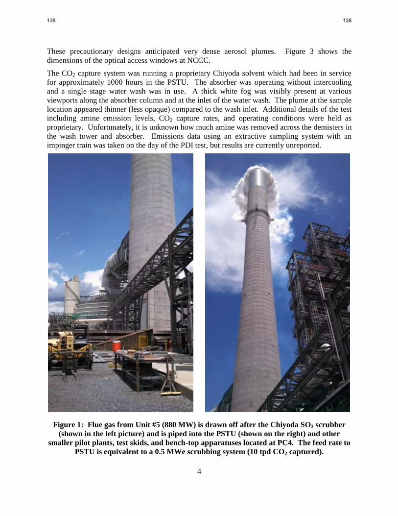
4

These precautionary designs anticipated very dense aerosol plumes. Figure 3 shows the

dimensions of the optical access windows at NCCC.

The CO2 capture system was running a proprietary Chiyoda solvent which had been in service

for approximately 1000 hours in the PSTU. The absorber was operating without intercooling

and a single stage water wash was in use. A thick white fog was visibly present at various

viewports along the absorber column and at the inlet of the water wash. The plume at the sample

location appeared thinner (less opaque) compared to the wash inlet. Additional details of the test

including amine emission levels, CO2 capture rates, and operating conditions were held as

proprietary. Unfortunately, it is unknown how much amine was removed across the demisters in

the wash tower and absorber. Emissions data using an extractive sampling system with an

impinger train was taken on the day of the PDI test, but results are currently unreported.

Figure 1: Flue gas from Unit #5 (880 MW) is drawn off after the Chiyoda SO2 scrubber

(shown in the left picture) and is piped into the PSTU (shown on the right) and other

smaller pilot plants, test skids, and bench-top apparatuses located at PC4. The feed rate to

PSTU is equivalent to a 0.5 MWe scrubbing system (10 tpd CO2 captured).

138 138

5

Figure 2: Optical access windows downstream of the water wash column. The gas flow is

oriented downward. The viewing cones inside of the flanges are flushed with N2 entering

from the top to prevent excessive window condensation. A liquid drain line is available at

the bottom of each flanged window.

The modular PDI system provided by Artium for the June 5 test had an additional beam

expander for the transmitter to increase the beam crossing angle to 28.1° in the vertical plane.

The custom-built beam expander was constructed of adjustable lenses attached to the mounting

rail. Prior to testing on the PSTU, the beams from the transmitter and the receiver had to be

aligned to the designed focal lengths of 350 and 500 mm for the transmitter and receiver,

respectively. A small, pocket-sized nebulizer was used to demonstrate the efficacy of the

transmitter/receiver system with an ad hoc beam expander for a dense particle cloud containing

0.1–20 μm droplets. The PDI analyzer measured a well-behaved, log-mean particle distribution

with a count-mean diameter of around 5 μm. The nebulizer fog was shown to be well within the

measuring capabilities of the PDI.

The analyzer and peripherals were then repacked and lifted by crane to the 6th

floor landing of

the PSTU and hand-carried the rest of the way to the 8th

floor where the water wash and duct

work are located. The equipment was secured on the support with C-clamps and quickly

realigned. Figure 4 shows the PDI setup prior to data collection. The transmitter and beam

expander are located in the foreground and the receiver is in the background. Figure 5 shows a

view of the beam crossing at the center of the duct and the detector output displayed on an

139 139

6

oscilloscope. A closer view of the beam crossing can be seen in Figure 6. The significant haze

surrounding the beams indicates a high concentration of particles scattering light.

Figure 3: Dimensions of the optical access windows on the PSTU. The viewing cones are

designed to accommodate the crossing angles of the transmitter and receiver.

Figure 4: The PDI transmitter (foreground) and receiver (background) mounted to

support rails prior to data collection.

140 140

7

Figure 5: Receiver output to an oscilloscope. The oscilloscope display shows a noisy

baseline for both detectors with no discreet Doppler bursts, indicating a high concentration

of particles ≤ 1 μm.

Figure 6: Close-up view of the transmitted beam crossing. The intersection of the laser

beams is where the gas is sampled for moving particles. 50 μm diameter beams were used

in this test.

141 141

8

Results

The PDI analyzer was unable to measure a particle size distribution inside the water wash outlet

duct due to a high concentration of particles ≤ 1 μm. Droplets and larger aerosols were visibly

present but were not measured by the instrument. The operability of the analyzer was

reconfirmed by measuring the particle size distribution of the nebulizer on the wooden support

structure built around the water wash duct. The test confirmed the same result as previously

measured.

Without emission data from the Chiyoda campaign it is difficult to assess to what extent aerosols

increased amine loss in the absorber and out of the water wash. Though there was a high

concentration of submicron particles, the significant portion of carryover may still reside in

particles ≥ 1 μm in diameter. Fog appeared to increase in opacity moving upwards in the

absorber and into the water wash; however, the fog looked visually thinner at the water wash

outlet. It is possible that significant particle loss occurs in the water wash, but this observation

needs to be confirmed through measurement.

Artium suggested that focusing the transmitted lasers to 2–5 μm in diameter (50 μm was used in

this test) would increase signal response at higher particle concentrations; however, the optical

path length would need to be reduced. The PDI analyzer may be able to measure particle size

distributions on smaller bench-scale systems but would require duct work modification to be

used at the pilot scale. A pilot plant’s exhaust would need to be split with a bypass line

somewhere around 1.5” in diameter to support a smaller and more focused PDI setup.

Conclusions

The modular PDI analyzer with transmitter beam expander was unsuccessful at measuring the

particle size distribution in the outlet duct from the water wash column at the PSTU located at

NCCC in Alabama. A high concentration of aerosols ≤ 1 μm precludes measurement of larger

droplets. However, due to the proprietary nature of the Chiyoda campaign, it is unclear what the

total amine emissions were and to what extent aerosols contributed. Particle collection across

the water wash is also unknown from these measurements.

Aerosols comprise a non-negligible portion of the total emitted amine. Emissions models must

include the mass contained in the aerosolized phase to correctly predict particle growth and,

subsequently, total emissions. The rate of aerosol growth depends on the rate at which amine

can transfer from the bulk liquid, through the bulk gas, and condense on the aerosol. High

concentrations of submicron particles indicate that coagulation may still be a significant

mechanism of aerosol growth throughout the absorber and water wash.

Future Work

Artium has proposed testing the Self-Contained PDI system on a bench-scale absorber with

thinner lasers, roughly 2–5 μm in diameter, to determine if the instrument is capable of

measuring larger particles in the presence of a submicron particle background at high

concentrations. The aerosol growth column represents an ideal test unit. If successful at the

bench scale, the outlet duct of the pilot plant at Pickle Research Campus will be modified for

aerosol measurements during future campaigns.

142 142

9

The aerosol growth column support structure is built and most instrumentation is connected.

Once parts are returned from welding and fabrication, gas and liquid lines can be connected and

controllers will be tested.

Acknowledgements

The authors wish to acknowledge the collaborative effort between NCCC, SRI, and Artium

Technologies undertaken to test the PDI analyzer. NCCC and SRI provided access to their pilot

plant and invested in modifications to their pilot plant to test the PDI analyzer. Artium

Technologies provided test equipment and technical support.

References

Mitsubishi Heavy Industries (MHI). “Amine Emission Control Technology of KM CDR

ProcessTM

.” Presented at the Amine Workshop in Palo Alto, California. August 16, 2011.

National Carbon Capture Center (NCCC). “National Carbon Capture Center: Post Combustion.”

Presented at the 2012 NETL CO2 Capture Technology Meeting. July 10, 2012.

Netherlands Organization for Applied Scientific Research (TNO). “Emission Reducing

Technologies Aerosols.” Presented at UTCCS-1 in Austin, Texas. January 25, 2012.

Rochelle et al. "CO2 Capture by Aqueous Absorption: Fourth Quarterly Progress Report 2012."

Luminant Carbon Management Program, 2013.

SINTEF. “Emission Studies at the Maasvlakte CO2 Capture Pilot Plant.” Presented at UTCCS-1

in Austin, Texas. January 25, 2012.

143 143

1

Amine Degradation in Pilot Plants


by Paul Nielsen




July 31, 2013

Abstract

A long-duration pilot plant campaign using PZ was conducted by CSIRO at the Tarong coal-

fired power plant in Australia. After 700 hours of parametric testing, steady state operation was

conducted with stripper sump operating temperatures 120 °C and 155 °C for 420 hours each.

During the 120 °C run, formate and its formamide accumulated at a rate of 0.056 mmol/kg/hr.

This increased to 0.17 mmol/kg/hr after the stripper temperature was raised. The rate of stainless

steel metal ion accumulation due to corrosion also increased significantly from 0.14 to 1.0

μmol/kg/hr when the stripper temperature was raised.

MNPZ in the Tarong solvent reached a steady state of approximately 7 mmol/kg after 7 weeks

with the stripper operating at 120 °C. After raising the stripper temperature to 155 °C the MNPZ

concentration dropped rapidly down towards a new steady state of 2 mmol/kg. Both

observations are in line with what was predicted using the model developed for MNPZ

decomposition.

For PZ cycled from 55 to 150 °C between a thermal and oxidative reactor in the HTCS cycling

apparatus, 75% of the nitrogen loss could be accounted for by the accumulation of ammonia,

formate, FPZ, 2-piperazinol (2-PZOH), ethylenediamine (EDA), volatile loss of PZ, and other

observed degradation products. This is a significant improvement over a previous material

balance done for PZ cycling oxidation in the ISDA, which could only quantify 27% of PZ

decomposition, but which did not measure volatile ammonia loss.

1-methylpiperazine was observed to form from the cycled oxidation of PZ in the HTCS and pilot

plants. This was shown in a bench-scale thermal degradation experiment to be the result of the

reaction and subsequent thermal decomposition of PZ and formaldehyde.

Introduction

Piperazine (PZ) has shown promise as a solvent for carbon dioxide capture, with greater

capacity, absorption rate, and thermal and oxidative stability than the baseline

monoethanolamine (MEA) solvent. However, PZ degradation is not as thoroughly characterized

as MEA, with a significant portion of the mass balance still unidentified (Freeman, 2011).

144 144

2

Tarong long-duration PZ campaign

CSIRO conducted a long-duration pilot plant campaign at the Tarong coal-fired power plant

using 8 m PZ. Liquid samples of lean and rich solvent, wash water, and stripper condensate

were collected weekly and analyzed for degradation product accumulation. A list of samples

received and analyzed is shown below in Table 1. During the first 856 hours of operation,

operating variables such as L/G and stripper operating temperature were varied. After this, the

stripper operating temperature was set to 120 °C and other process variables were held constant

for a long-duration run of 425 hours. The stripper operating temperature was then raised to

155 °C kept constant for another 421 hours.

Table 1: Samples received and analyzed from Tarong pilot plant PZ campaign

Date Hours of operation

11/15/2012 749.1

11/22/2012 781.3

11/29/2012 839.9

12/4/2012 855.6

12/13/2012 927.5 120 °C

12/20/2012 986

1/10/2013 1078.4

1/17/2013 1178.6

1/24/2013 1229.9

2/22/2013 1280.6

2/28/2013 1327.0 155 °C

3/5/2013 1376.6

3/7/2013 1424.6

3/13/2013 1475

3/15/2013 1514.1

3/21/2013 1601.7

3/28/2013 1676

4/3/2013 1701.7

Table 2: Typical flue gas composition at Tarong (average of Line 6 FTIR analysis, 11/15–

1/14)

Water vapor H2O 5.00 vol %

Carbon dioxide CO2 11.90 vol %

Oxygen O2 6.94 vol %

Nitrogen N2 76.16 vol %

Carbon monoxide CO 47.71 ppm

NOx 210.20 ppm

Nitrogen oxide NO 208.92 ppm

Nitrogen dioxide NO2 1.28 ppm

Sulfur dioxide SO2 0.55 ppm

Sulfur trioxide SO3 0.002 ppm

145 145

3

Ammonia NH3 0.49 ppm

Hydrogen chloride HCl 0.32 ppm

Hydrogen fluoride HF 1.79 ppm

Degradation and reclaiming modeling

The Texas Carbon Management Program in coordination with Trimeric and URS has conducted

a review of solvent reclaiming technologies. The project is sponsored by IEAGHG. TCMP’s

contribution to the review is a complete survey and analysis of solvent degradation in order to

determine the composition of both the feed to the reclaimer and the sludge waste products that

must be treated.


A full description of the High Temperature Oxidation Reactor (HTOR or HTCS) can be found in

Alex Voice’s recent Ph.D. dissertation (Voice, 2013)

Analytical Methods

All analytical methods used have been discussed in previous quarterly reports (Rochelle et al.,

2013).

Safety: International Shipping of Pilot Plant Samples

Samples from Tarong in Australia were shipped in 30+ mL vials. The vials were sealed with

tape, and were then placed in sealed bags and packed with packing material in cardboard boxes

before being shipped. Upon arrival in Austin, TX, the samples were opened inside a fume hood

to vent any vapor buildup that may have occurred. No samples leaked in transit.


Tarong High Temperature PZ Campaign Results

Figure 1 shows the accumulation of formate, stainless steel metal ions (SSM), 2-piperazinol (2-

PZOH), and ethylenediamine (EDA) during the long-duration runs conducted at Tarong. The

rate of formate accumulation increased from 0.056 to 0.166 mmol/kg/hr when the stripper

temperature was raised from 120 °C to 155 °C. The rate of SSM accumulation from corrosion

follows a similar trend. The SSM ions may be catalyzing degradation, the formate accumulation

may be catalyzing corrosion, or there may be a synergistic effect between the two trends. 2-

PZOH and EDA are intermediate degradation products and do not show any long term trends.

146 146

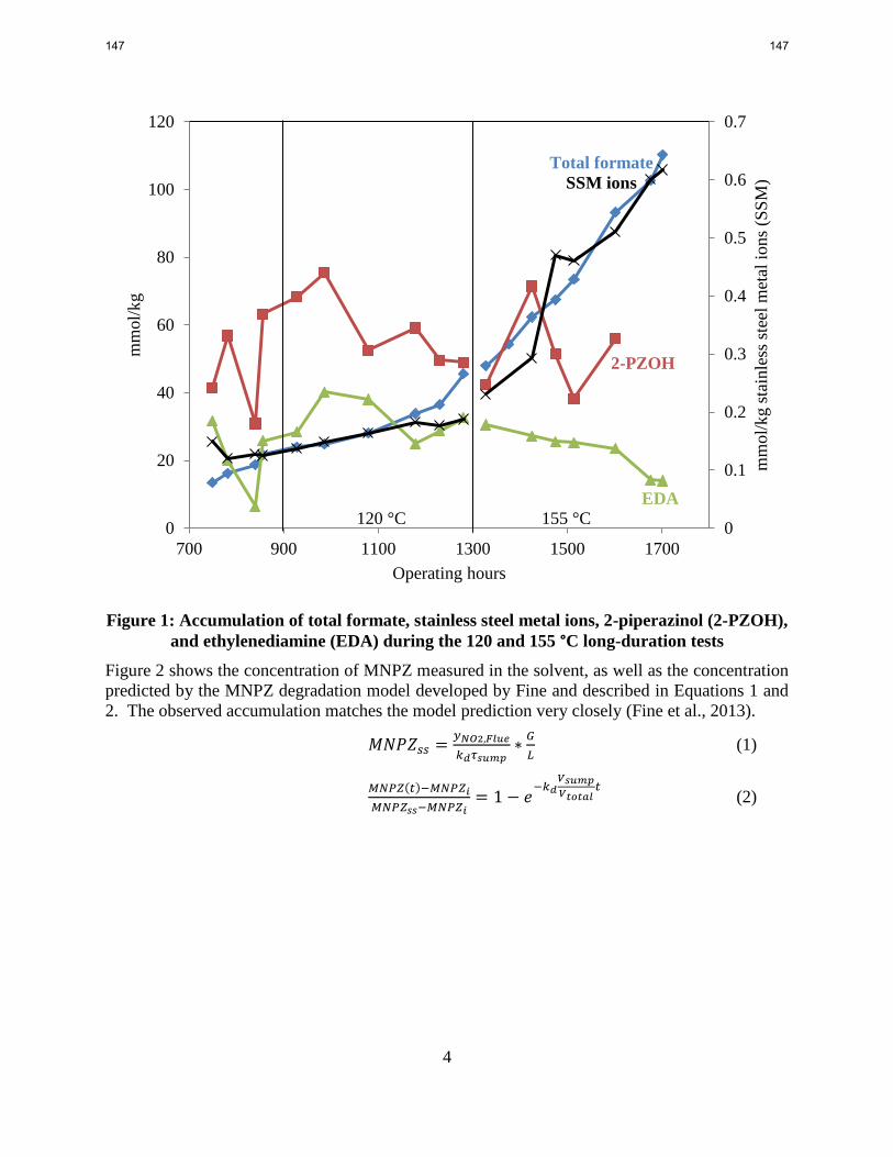
4

Figure 1: Accumulation of total formate, stainless steel metal ions, 2-piperazinol (2-PZOH),

and ethylenediamine (EDA) during the 120 and 155 °C long-duration tests

Figure 2 shows the concentration of MNPZ measured in the solvent, as well as the concentration

predicted by the MNPZ degradation model developed by Fine and described in Equations 1 and

2. The observed accumulation matches the model prediction very closely (Fine et al., 2013).

(1)

( )

(2)

0

0.1

0.2

0.3

0.4

0.5

0.6

0.7

0

20

40

60

80

100

120

700 900 1100 1300 1500 1700

mm

ol/

kg s

tain

less

ste

el m

etal

ions

(SS

M)

mm

ol/

kg

Operating hours

EDA

2-PZOH

Total formate

SSM ions

120 °C 155 °C

147 147

5

Figure 2: Measured and predicted concentration of MNPZ in lean and rich solvent

samples. Model parameters: NO2 in the flue gas yNO2 = 1.2 ppmv, residence time in the

stripper τsump = 8 minutes, MNPZ degradation rate constant kd calculated from stripper

operating temperature of 120–150 °C, L/G = 2.2 wt/wt, stripper hold-up Vsump/Vtotal = 0.25

Figure 3 shows the accumulation of nitrate and sulfate in the solvent from the absorption of NOx

and SOx from the flue gas. The absorption rate of these contaminants is not a function of the

stripper operating temperature. Nitrate absorbs continuously at a rate of 0.016 mmol/kg/hr.

Sulfate accumulation seems to be slower, but punctuated by sudden increases, possibly due to

minor process upsets in the pilot plant prescrubber unit.

0

1

2

3

4

5

6

7

8

700 900 1100 1300 1500 1700

MN

PZ

in S

olv

ent

(mm

ol/

kg)

Hours

Lean

Rich

Model Prediction

148 148

6

Figure 3: Accumulation of nitrate and sulfate. Inlet flue gas composition: 200 ppm NOx,

0.5 ppm SOx

Table 3: Rates of degradation product and contaminant accumulation for 120 and 155 °C

runs at Tarong and calculated activation energy of formation

120 °C 155 °C Ea

mmol/kg/hr kJ/mol

Total formate 0.056 0.166 44

Total acetate 0.009 0.024 38

Total oxalate 0.013 -0.011

AEP 0.0006 0.0025 55

U 34.8 min (1MPZ?) 0.0024 0.0127 66

Sulfate 0.018 0.012

Nitrate 0.017 0.015

Fe2+ 1.15*10-4

9.37*10-4

84

Cr3+ 1.96*10-6

3.75*10-5

118

Ni2+ 1.14*10-5

4.93*10-5

59

Total SSM ions 1.40*10-4

1.03*10-3

80

Table 4 shows the composition of the lean solvent at Tarong at the end of the 120 °C and 155 °C

runs compared to previously analyzed PZ solvents from campaigns at SRP in Austin, TX, and at

Pilot Plant 2 (PP2). The SRP campaign used a synthetic flue gas of 12 kPa CO2 in air, while PP2

used a slipstream from a coal-fired power plant, as did Tarong (Rochelle et al, 2013).

0

5

10

15

20

25

30

35

700 900 1100 1300 1500 1700

mm

ol/

kg

Hours

Sulfate

Nitrate

149 149

7

The campaign conducted at Tarong was the longest of the three campaigns and saw the largest

accumulation of degradation products. The profile of degradation products observed at Tarong

was very similar to what was observed at PP2. Heat stable salts did not accumulate in the

solvent at SRP, likely due to the lack of corrosion to catalyze degradation.

The component labeled “U 34.8 min” is a peaked observed to elute after PZ in the cation IC.

Based on its elution time it may be 1-methylpiperazine (1MPZ). In previous quarterly reports

with results from SRP and PP2 this peak was misidentified as 1-hydroxyethyl-piperazine (HEP).

It will be discussed in further detail later in the report.

Table: Final solvent composition at end of campaigns at SRP and PP2, and solvent

composition at Tarong at end of 120 °C long-duration run and 155 °C long-duration run

Pilot plant: SRP PP2 Tarong

Stripper temperature:

(mmol/kg)

135–150 °C

(1400 hrs)

150 °C 120 °C

(1281 hrs)

155 °C

(1702 hrs)

Total alkalinity 4112 4132 4125 4062

Piperazine (Cation IC) 3855 3546 4119 3927

Total formate 2.4 76.6 45.6 110.2

N-formyl-PZ (FPZ) 1.3 38.0 12.8 58.9

Total acetate 0.3 11.2 5.2 14.6

Total oxalate 0.3 8.6 6.2 2.7

Ammonium (NH4+

) N/A 0.7 1.0 0.3

Ethylenediamine (EDA) 12.8 9.3 32.6 14.0

N-aminoethyl-PZ (AEP) 3.6 2.9 0.9 1.6

U 34.8 min (1MPZ?) 2.2 2.6 3.9 9.3

MNPZ 0.09 1.2 7.19 2.44

2-PZOH 25.8 71.6 48.9 56.0

Sulfate 0 7.1 23.0 26.9

Nitrate 0.1 4.8 16.9 21.8

Fe2+

0.02 1.13 0.15 0.54

Cr3+

0.02 2.21 0.016 0.032

Ni2+

0.02 1.86 0.014 0.034

Mn2+

0.004 0.15 0.008 0.011

Total SSM ions 0.06 5.35 0.188 0.617

Table 5 compares the accumulation of contaminants in the final samples of wash water and

stripper condensate at Tarong to what was previously observed at PP2. The stripper condensate

at Tarong was recycled to the top of the stripper, creating its own wash and limiting

accumulation of contaminants to the μmol/kg level (less than 10 ppmw).

Of interest is the “volatility ratio,” which is the ratio of contaminant concentration relative to PZ

in the wash relative to the solvent. Contaminants with a ratio greater than 1 are theoretically

more volatile than PZ, and are relatively more concentrated in the wash or condensate. For

example, ammonium is around 90 times more concentrated compared to PZ in the wash relative

to the solvent. MNPZ is about equally as concentrated. The component believed to be 1MPZ is

30 to 40 times more concentrated. 1MPZ is known to be significantly more volatile than PZ.

150 150

8

(

)

(

)

(3)

Table 5: Concentration of contaminants in final wash water sample of PP2 and Tarong PZ

campaigns and stripper condensate at Tarong. Volatility ratio: ratio of contaminant to PZ

in wash water or condensate to solvent

PP2 Tarong

Wash

mmol/kg

Volatility

ratio

Wash

mmol/kg

Volatility

ratio

Stripper

Condens.

μmol/kg

Volatility

ratio

Piperazine (cation IC) 33.0 1 62.0 1 110 1

N-formyl-PZ 0.08 0.09 0.8 0.5

Ammonium 0.61 94.8 0.41 85.8 0.09 10

Ethylenediamine 0.12 0.56 0.2 0.5

U 34.8 min (1MPZ?) 0.76 30.9 5.02 34.3 10 39

MNPZ 0.02 1.76 0.03 0.73

HTOR8: 8 m PZ Oxidation Cycled from 55 to 150 °C

A two-week experiment was conducted in the High Temperature Oxidative Reactor apparatus

(HTOR) cycling PZ from 55 °C in an oxidation reactor to 150 °C in a thermal reactor with

stainless steel metal ions added to the solvent to catalyze oxidation. Figure 4 shows the decrease

in PZ and total alkalinity observed over the campaign. The decrease can be attributed to

degradation, volatility loss, and changes in the water balance. The water balance was controlled

by sparging with saturated air and using a condenser to keep a constant solvent inventory.

Over the course of the experiment, the concentration of PZ in the solvent decreased by

approximately 350 mmol/kg, after adjusting for changes in the water balance and makeup

solvent added during the experiment.

151 151

9

Figure 4: Piperazine concentration in HTOR8: 8 m PZ, oxidative reactor at 55 °C sparged

with 7 L/min 2 kPa CO2 in air, cycled to 150 °C, 0.2 L/min circulation rate, 2 weeks

Figures 5 and 6 show the accumulation of all observed degradation products in the solvent

during the experiment. The solvent had already been degraded slightly before the start of the

experiment. Formate, 2-PZOH, EDA, and 1MPZ were the most significant liquid-phase

products observed. The accumulation of acetate, oxalate, and MNPZ followed similar trends to

formate at lower concentrations. Intermediate products 2-PZOH and EDA decreased in

concentration over the course of the campaign.

3450

3500

3550

3600

3650

3700

3750

3800

3850

3900

3950

0 50 100 150 200 250 300 350

mm

ol/

kg

Hours

Total Alkalinity

PZ (Cation IC)

152 152

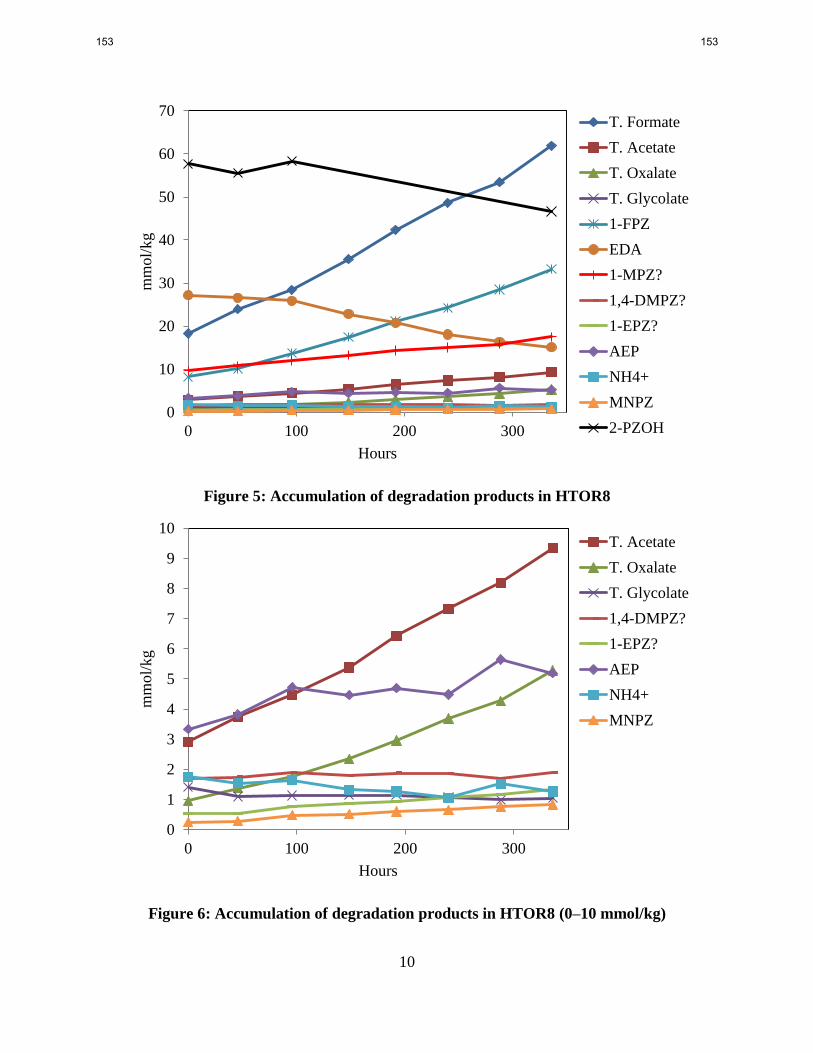
10

Figure 5: Accumulation of degradation products in HTOR8

Figure 6: Accumulation of degradation products in HTOR8 (0–10 mmol/kg)

0

10

20

30

40

50

60

70

0 100 200 300

mm

ol/

kg

Hours

T. Formate

T. Acetate

T. Oxalate

T. Glycolate

1-FPZ

EDA

1-MPZ?

1,4-DMPZ?

1-EPZ?

AEP

NH4+

MNPZ

2-PZOH

0

1

2

3

4

5

6

7

8

9

10

0 100 200 300

mm

ol/

kg

Hours

T. Acetate

T. Oxalate

T. Glycolate

1,4-DMPZ?

1-EPZ?

AEP

NH4+

MNPZ

153 153

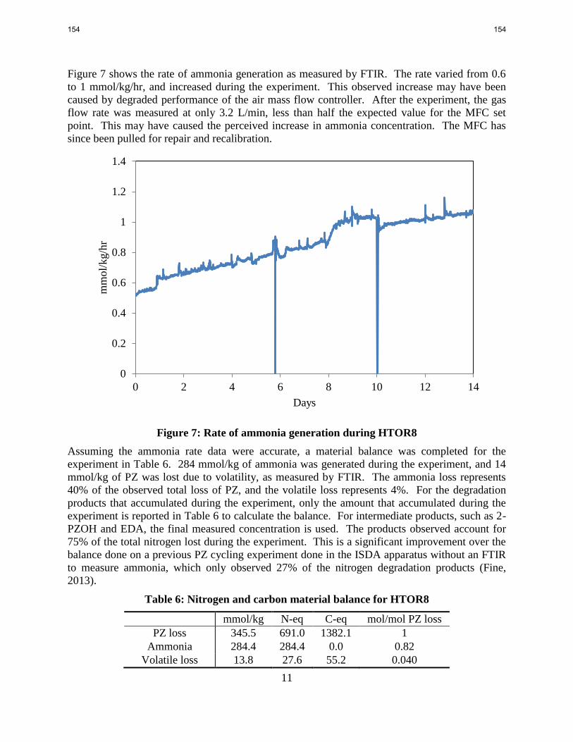
11

Figure 7 shows the rate of ammonia generation as measured by FTIR. The rate varied from 0.6

to 1 mmol/kg/hr, and increased during the experiment. This observed increase may have been

caused by degraded performance of the air mass flow controller. After the experiment, the gas

flow rate was measured at only 3.2 L/min, less than half the expected value for the MFC set

point. This may have caused the perceived increase in ammonia concentration. The MFC has

since been pulled for repair and recalibration.

Figure 7: Rate of ammonia generation during HTOR8

Assuming the ammonia rate data were accurate, a material balance was completed for the

experiment in Table 6. 284 mmol/kg of ammonia was generated during the experiment, and 14

mmol/kg of PZ was lost due to volatility, as measured by FTIR. The ammonia loss represents

40% of the observed total loss of PZ, and the volatile loss represents 4%. For the degradation

products that accumulated during the experiment, only the amount that accumulated during the

experiment is reported in Table 6 to calculate the balance. For intermediate products, such as 2-

PZOH and EDA, the final measured concentration is used. The products observed account for

75% of the total nitrogen lost during the experiment. This is a significant improvement over the

balance done on a previous PZ cycling experiment done in the ISDA apparatus without an FTIR

to measure ammonia, which only observed 27% of the nitrogen degradation products (Fine,

2013).

Table 6: Nitrogen and carbon material balance for HTOR8

mmol/kg N-eq C-eq mol/mol PZ loss

PZ loss 345.5 691.0 1382.1 1

Ammonia 284.4 284.4 0.0 0.82

Volatile loss 13.8 27.6 55.2 0.040

0

0.2

0.4

0.6

0.8

1

1.2

1.4

0 2 4 6 8 10 12 14

mm

ol/

kg/h

r

Days

154 154

12

Total formate 43.3 0.13

FPZ 25.1 50.2 125.5 0.073

Free formate 18.2 18.2 0.053

Acetate 6.4 12.8 0.018

PZ-oxalyl amide 4.2 8.5 25.5 0.012

Glycolate 3.1 6.1 0.009

EDA 15.1 30.2 30.2 0.044

1MPZ 7.5 15.0 37.6 0.022

AEP 1.8 5.4 10.8 0.005

1,4-DMPZ 0.8 1.7 5.0 0.002

1EPZ 0.1 0.2 0.6 0.0003

Ammonia 1.3 1.3 0.004

MNPZ 0.6 1.8 2.4 0.002

2-PZOH 46.2 92.4 184.8 0.13

Balance 75% 37%

Identification of 34.8 Minute Cation Peak

In all the pilot plant and cycling apparatus PZ samples, a peak was observed to elute in the cation

IC immediately after PZ, at 34.8 minutes. This peak is labeled “U 34.8 min” in this report. This

is the same elution time as 1MPZ. 1MPZ had not been previously expected to form as a result of

PZ degradation, and has not been previously observed in bench-scale thermal degradation or low

temperature oxidation experiments (Freeman, 2011). A possible pathway for its formation is

proposed in Figure 8. PZ reacts with formaldehyde to form a methyl-piperazine polymer foam,

which has been observed in previous low temperature oxidation experiments when formaldehyde

is added (Freeman, 2013). If this is heated, the compound may then decompose to 1MPZ and 2-

PZOH. This could only occur if the solvent is cycled from a low temperature oxidizing

environment to a high temperature reducing environment, as occurs in pilot plants and the

HTCS.

To test this theory, 100 mmol/kg of formaldehyde was added to fresh 8 m PZ in a thermal

cylinder and heated to 135 °C for 24 hours, along with a pure 8 m PZ control sample. The

resulting product did not contain any observable foam polymer, and had turned dark yellow. A

large peak was observed in the cation IC at 34.8 minutes, corresponding to 25 mmol/kg of

1MPZ. The concentration of PZ decreased 190 mmol/kg, indicating that 1 mole of formaldehyde

reacted with 2 moles of PZ, as predicted. Free formaldehyde was not observed in the degraded

sample. Based on this, formaldehyde reacted fully with the PZ, and then partially decomposed to

1MPZ. Other unquantified PZ-formaldehyde complexes and polymers probably exist. The clean

8 m PZ control sample was clear, did not have a significant decrease in PZ concentration, and no

peak was observed at 34.8 minutes.

Direct injection mass spectroscopy of the thermally degraded PZ-formaldehyde sample did not

detect 1MPZ. However, a more complete analysis using IC-MS or GC-MS will be conducted.

If 1MPZ can form from the cycling degradation of PZ and formaldehyde, then 1,4-dimethyl-PZ

(1,4-DMPZ) and 1-ethyl-PZ (1EPZ) should also be expected to form. 1EPZ could form from the

155 155

13

reaction and decomposition of PZ and acetaldehyde. Cation IC peaks corresponding to the

elution times for 1,4-DMPZ and 1EPZ were observed in the HTOR8 PZ cycling experiment.

Figure 8: Proposed reaction pathway for the formation of 1MPZ and 2-PZOH from high

temperature cycling of PZ and formaldehyde

Conclusions

In the long-duration PZ campaign conducted at Tarong in Australia, formate accumulation and

corrosion were a strong function of the stripper operating temperature. Total formate

accumulation rate increased from 0.056 to 0.166 mmol/kg/hr and the corrosion rate increased

from 0.14 to 1.0 μmol/kg/hr when the stripper temperature was raised from 120 °C to 155 °C.

MNPZ accumulation at Tarong matched model predictions, decreasing from 7 mmol/kg to 2

mmol/kg as a result of increased thermal decomposition when the stripper temperature was

raised.

Ammonium and 1MPZ accumulated in the wash water and stripper condensate at Tarong at a

significantly larger relative concentration compared to PZ in the solvent, indicating that these

two contaminants are more volatile than PZ. 1MPZ was 34 times more concentrated, while

156 156

14

ammonium was 86 times more concentrated in the final wash water sample. MPNZ and FPZ

were not as concentrated in the wash and condensate compared to PZ, demonstrating that they

are less volatile than PZ.

In PZ cycled from 55 to 150 °C in the HTCS cycling apparatus, 75% of the nitrogen loss could

be accounted for by the accumulation of ammonia, formate, FPZ, 2-piperazinol (2-PZOH),

ethylenediamine (EDA), and other observed degradation products.

A cation IC peak corresponding to the elution time and with similar volatility to 1MPZ was

observed in degraded PZ from pilot plant campaigns and the cycling apparatus experiment.

When 100 mmol/kg formaldehyde was added to PZ and heated to 135 °C, it reacted with 190

mmol/kg PZ to produce 25 mmol/kg 1MPZ. There may be other unidentified PZ-formaldehyde

complexes.

Future Work

GC-MS and IC-MS will be conducted on the thermally decomposed PZ-formaldehyde sample to

confirm the presence of 1MPZ. A similar experiment using acetaldehyde will be conducted to

see if 1EPZ can be produced.

Solvent screening on the high temperature cycling system will be conducted. This will include a

repeat of the 8 m PZ experiment cycled from 55 to 150 °C; an experiment to see the effects of

nitrogen sparging to remove dissolved oxygen before the high temperature reactor in order to

reduce oxidation; the addition of sodium nitrite to observe MNPZ formation and decomposition;

and a test of 7/2 m MDEA/PZ and other solvents.

The effect on viscosity of the addition of up to 1 M formate and sulfate to 7 m MEA and 8 m PZ

will be determined.

Additional refinement and validation will be made on the degradation models developed for

MEA and PZ.

Acknowledgements

CSIRO wishes to acknowledge financial assistance provided through Australian National Low

Emissions Coal Research and Development (ANLEC R&D). ANLEC R&D is supported by

Australian Coal Association Low Emissions Technology Limited and the Australian Government

through the Clean Energy Initiative.

References

Freeman SA. Thermal Degradation and Oxidation of Aqueous Piperazine for Carbon Dioxide

Capture. The University of Texas at Austin. Ph.D. Dissertation. 2011.

Fine NA, Goldman MJ, Nielsen PT, Rochelle GT. "Managing n-nitrosopiperazine and

dinitrosopiperazine." GHGT-11. Kyoto, Japan. 2012.

Rochelle GT et al. “CO2 Capture by Aqueous Absorption, First Quarterly Progress Report 2013.”

Texas Carbon Management Program. The University of Texas at Austin. 2013.

Voice AK. Amine Oxidation in Carbon Dioxide Capture by Aqueous Scrubbing. The University

of Texas at Austin. Ph.D. Dissertation. 2013.

157 157

1

Nitrosamine yield in MEA, PZ, and PZ blends


by Nathan Fine




July 31, 2013

Abstract

This quarter nitrosation kinetics were determined for primary, secondary, and tertiary amines.

Nitrosation is first order in nitrite, total amine, and hydronium ion concentration and catalyzed

by carbamate species. Therefore nitrosation is much faster in the carbamate-forming primary

and secondary amines than tertiary and hindered amines. Nitrosamine kinetics were also

measured for hydroxyethyl-glycine (HeGly) and hydroxyethyl-ethylenediamine (HEEDA) two

known degradation products of monoethanolamine (MEA). HeGly nitrosates 4.6 times more

readily than MEA under stripper conditions with weak dependencies on loading and temperature.

HEEDA nitrosates 2.8 times more readily than MEA at 120 °C with nitrosation rates dropping to

2.2 times that of MEA at 150 °C.

Total nitrosamine (TONO) concentration for degraded PZ from PP2 and Tarong matched

previous HPLC results for MNPZ, so there are no other significant nitrosamines in PZ.

Degraded MEA samples from NCCC, SRP, and TNO had between 0.1 and 0.3 mmol/kg of total

nitrosamine, which is about 10 times less than the nitrosamine content in PZ. However,

nitrosamine concentration in MEA had not necessarily reached steady state. The degraded MEA

sample from TNO was reacted with 0.37 mol/kg nitrite and analyzed on both the HPLC and the

total nitrosamine (TONO) apparatus. Total nitrosamine yield was 4.6% with NHeGly making up

49% of the total nitrosamine, NDELA making up 31%, and no NHEEDA detected. The yield to

nitrosodiethanolamine (NDELA) was most likely inflated by the formation of diethanolamine

(DEA) from nitrosated MEA during the experiment. The balance of the total nitrosamine could

be from nitrosated iso-4-(2-hydroxyethyl)piperazin-2-one (iso-HEPO) or 2-Hydroxyethyl-

(2-hydroxyethylamino)acetamide (HEHEAA), two secondary amines derived from HeGly.

The Nitrosamine Cycle

Figure 1 gives a proposed sequence of processes that determine nitrosamine accumulation in

amine scrubbing. Flue gas containing NO2 enters a polishing scrubber where a fraction (α) of the

NO2 can be removed via reaction with sulfite. The remaining NO2 then enters the absorber

where a portion (β) of it can absorb into the amine solution as nitrite. Another portion (γ) can

undergo a 2-phase reaction with a secondary amine to directly form a nitrosamine; the rest of the

NO2 will vent from the absorber along with the scrubbed flue gas. Amine oxidation is another

source of nitrite in amine solvents that are not oxidatively stable such as MEA. Nitrite from NO2

158 158

2

absorption and amine oxidation will then travel to the stripper where it can nitrosate a secondary

amine with a yield of δ. The yield is determined by the concentration of secondary amines in the

solvent and their relative nitrosation rates as compared to the principal amine. After nitrosation,

the nitrosamine will thermally decompose in the stripper sump according to a first order rate

constant (kstr). In many amine scrubbing systems, a slipstream (x) of the solvent is passed

through a distillation reclaimer to remove any nonvolatile impurities. Nitrosamines will also

accumulate in the reclaimer based on their volatilities (HNNO) and the thermal decomposition rate

constant in the reclaimer (kRecl). Assuming a well-mixed system, nitrosamine sources from NO2

absorption and amine oxidation will balance out with nitrosamine sinks from thermal

decomposition in the stripper and reclaimer to yield steady state nitrosamine concentration in the

stripper and the reclaimer (Equations 1 & 2). This report will focus on nitrosamine yield via

nitrosation from nitrite.

159 159

3

Figure 1: Nitrosamine Accumulation in Amine Scrubbing

( )

( )

(

)

(1)

(2)

SO2

Polishing

Scrubber

Stripper Absorber

𝑁𝑁𝑂𝑘𝑆𝑡𝑟 𝑃𝑟𝑜𝑑𝑢𝑐𝑡

𝛿𝑁𝑂2− 𝐴𝑚 → 𝑁𝑁𝑂 𝐻𝐶𝑂3

−

𝛾2𝑁𝑂2 𝐴𝑚 → 𝑁𝑁𝑂 𝑁𝑂3−

𝛽𝑁𝑂2 𝐴𝑚 → 𝑁𝑂2− 𝐴𝑚 ∙

𝑁𝑂2 𝑆𝑂32− → 𝑁𝑂2

− 𝑆𝑂2− ∙

Reclaimer

𝐴𝑚 𝑂∙ → 𝑁𝑂2−

𝑁𝑁𝑂𝑘𝑅𝑒𝑐𝑙 𝑃𝑟𝑜𝑑𝑢𝑐𝑡

𝑦𝑁𝑂 𝐹𝐿 ( 𝛼)𝑦𝑁𝑂 𝐹𝐿

𝛼𝑦𝑁𝑂 𝐹𝐿

( )( )

160 160

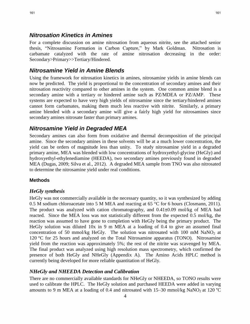
4

Nitrosation Kinetics in Amines

For a complete discussion on amine nitrosation from aqueous nitrite, see the attached senior

thesis, “Nitrosamine Formation in Carbon Capture,” by Mark Goldman. Nitrosation is

carbamate catalyzed with the rate of amine nitrosation decreasing in the order:

Secondary>Primary>>Tertiary/Hindered.

Nitrosamine Yield in Amine Blends

Using the framework for nitrosation kinetics in amines, nitrosamine yields in amine blends can

now be predicted. The yield is proportional to the concentration of secondary amines and their

nitrosation reactivity compared to other amines in the system. One common amine blend is a

secondary amine with a tertiary or hindered amine such as PZ/MDEA or PZ/AMP. These

systems are expected to have very high yields of nitrosamine since the tertiary/hindered amines

cannot form carbamates, making them much less reactive with nitrite. Similarly, a primary

amine blended with a secondary amine will give a fairly high yield for nitrosamines since

secondary amines nitrosate faster than primary amines.

Nitrosamine Yield in Degraded MEA

Secondary amines can also form from oxidative and thermal decomposition of the principal

amine. Since the secondary amines in these solvents will be at a much lower concentration, the

yield can be orders of magnitude less than unity. To study nitrosamine yield in a degraded

primary amine, MEA was blended with low concentrations of hydroxyethyl-glycine (HeGly) and

hydroxyethyl-ethylenediamine (HEEDA), two secondary amines previously found in degraded

MEA (Dugas, 2009; Silva et al., 2012). A degraded MEA sample from TNO was also nitrosated

to determine the nitrosamine yield under real conditions.

Methods

HeGly synthesis

HeGly was not commercially available in the necessary quantity, so it was synthesized by adding

0.5 M sodium chloroacetate into 5 M MEA and reacting at 65 °C for 6 hours (Closmann, 2011).

The product was analyzed with cation chromatography, and 0.41±0.09 mol/kg of MEA had

reacted. Since the MEA loss was not statistically different from the expected 0.5 mol/kg, the

reaction was assumed to have gone to completion with HeGly being the primary product. The

HeGly solution was diluted 10x in 9 m MEA at a loading of 0.4 to give an assumed final

concentration of 50 mmol/kg HeGly. The solution was nitrosated with 100 mM NaNO2 at

120 °C for 25 hours and analyzed on the Total Nitrosamine apparatus (TONO). Nitrosamine

yield from the reaction was approximately 5%; the rest of the nitrite was scavenged by MEA.

The final product was analyzed using high resolution mass spectrometry, which confirmed the

presence of both HeGly and NHeGly (Appendix A). The Amino Acids HPLC method is

currently being developed for more reliable quantitation of HeGly.

NHeGly and NHEEDA Detection and Calibration

There are no commercially available standards for NHeGly or NHEEDA, so TONO results were

used to calibrate the HPLC. The HeGly solution and purchased HEEDA were added in varying

amounts to 9 m MEA at a loading of 0.4 and nitrosated with 15–30 mmol/kg NaNO2 at 120 °C

161 161

5

for 18 hours. The final products were analyzed via TONO and then the HPLC. Trace nitrite and

other nitrosamines in the system were subtracted from the total nitrosamine amount by analyzing

the same reaction in the neat MEA solution. NHEEDA eluted in the HPLC method at t = 5.3

minutes with no large interferences in the matrix. NHeGly eluted in the void space (t = 2.1

minutes) of the column because it is charged under basic conditions. The main interference for

NHeGly is nitrite, which is subtracted from the peak area whenever necessary. Nitrite was very

low for the NHeGly calibration and made up less than 5% of the total peak area. Both NHEEDA

and NHeGly had linear responses on the HPLC with coefficients of determination greater than

0.999 (Appendix B). All subsequent experimental analysis for NHEEDA and NHeGly will be

done using the HPLC which allows for more rapid analysis than the TONO.

NHeGly and NHEEDA yield in MEA

Varying amounts of HeGly and HEEDA were added to solutions of loaded MEA and heated to

120 °C or 150 °C. All of the cylinders for an experimental set were removed at the same time

and quenched immediately to give nitrosamine yield as a function of secondary amine

concentration. The reaction time for each experimental set was a delicate balance between

maximizing nitrite consumption and minimizing nitrosamine decomposition. Nitrosation at

150 °C lasted 2–4 hours whereas nitrosation at 120 °C lasted 18–25 hours. In 9 m MEA at a

loading of 0.4, nitrosation was greater than 99% complete due to fast kinetics at high loadings.

However, in 7 m MEA at a loading of 0.17, nitrosation was only 40–60% complete. Since

HeGly and nitrite both elute in the void space of the HPLC method, the excess nitrite introduces

some error into those results. Nitrosamine yield was determined by Equation 3.

(3)

Safety

Nitrite reacts with MEA to form an unstable nitrosamine that immediately decomposes into N2

and a carbocation. Pressure builds up in the cylinders as the N2 evolves from the solution, and

the cylinder makes a hissing noise as it is opened due to the pressure releasing. To limit cylinder

pressurization, cylinders are only filled to 80% of their total volume for experiments with

primary amines. Cylinders are also opened slowly so the top does not pop off uncontrollably.

Results

HeGly

Nitrosamine yield was plotted against the relative concentrations of HeGly to MEA. Yield was

proportional to HeGly concentration with the slope of the line representing the relative

nitrosation rates of HeGly to MEA (Figure 2). The relative reactivity for HeGly decreases by

30% going from α = 0.17 to α = 0.4, which suggests that HeGly carbamate increases more

slowly than MEA carbamate across this loading (Figure 3). As the temperature increases from

120 °C to 150 °C, the relative reactivity of HeGly decreases by approximately 10–15%, yielding

a HeGly nitrosation activation energy 3–4 kJ/mol less than MEA. Since there is no carbamate

speciation data for this blend, the third order rate constant for HeGly nitrosation cannot be

determined.

162 162

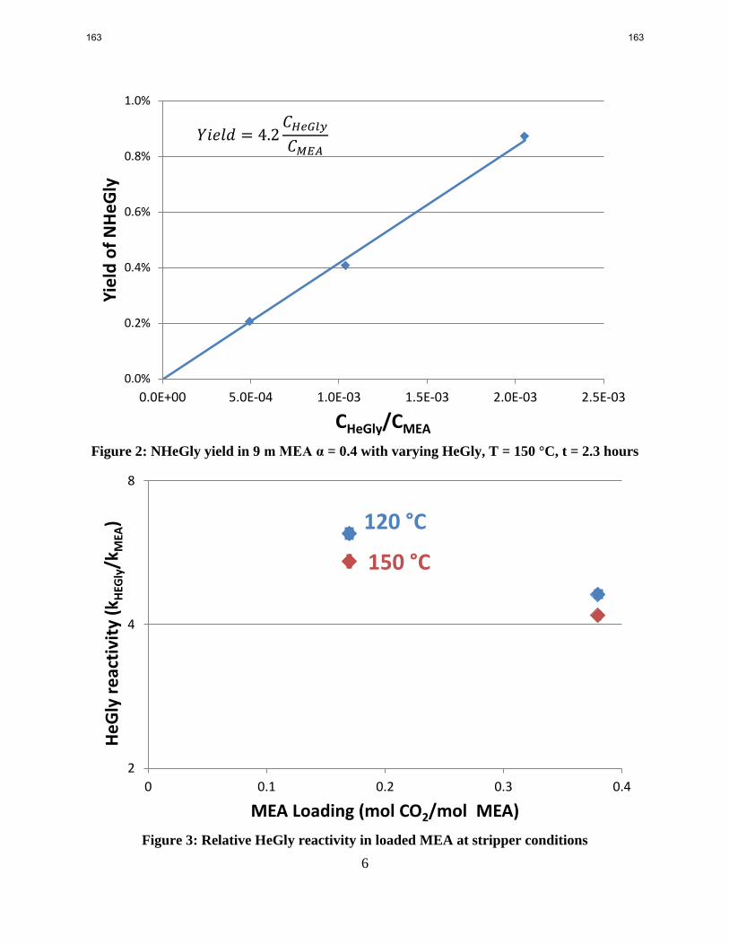
6

Figure 2: NHeGly yield in 9 m MEA α = 0.4 with varying HeGly, T = 150 °C, t = 2.3 hours

Figure 3: Relative HeGly reactivity in loaded MEA at stripper conditions

0.0%

0.2%

0.4%

0.6%

0.8%

1.0%

0.0E+00 5.0E-04 1.0E-03 1.5E-03 2.0E-03 2.5E-03

Yie

ld o

f N

He

Gly

CHeGly/CMEA

4.2 𝐻 𝐺 𝑦 𝑀𝐸𝐴

120 °C

150 °C

2

4

8

0 0.1 0.2 0.3 0.4

He

Gly

re

acti

vity

(k H

EGly

/kM

EA)

MEA Loading (mol CO2/mol MEA)

163 163

7

HEEDA

The same experimental set was carried out with HEEDA in MEA. Yield was again proportional

to HEEDA concentration (Figure 4). The relative reactivity for HEEDA was independent of

loading going from α = 0.17 to α = 0.4, so HEEDA carbamate forms at the same pace as MEA

carbamate in this range (Figure 5). As the temperature increases from 120 °C to 150 °C the

relative reactivity of HEEDA decreases by 25%%, yielding a HEEDA nitrosation activation

energy 8 kJ/mol less than MEA. Since there are no carbamate speciation data for this blend, the

third order nitrosation constant for HEEDA cannot be determined.

Figure 4: NHEEDA yield in 9 m MEA α = 0.38 with HEEDA, T = 150 °C, t = 3.3 hours

0%

2%

4%

6%

8%

0.0E+00 5.0E-03 1.0E-02 1.5E-02 2.0E-02 2.5E-02 3.0E-02 3.5E-02

Yie

ld o

f N

HEE

DA

CHEEDA/CMEA

2.2 𝐻𝐸𝐸𝐷𝐴 𝑀𝐸𝐴

164 164

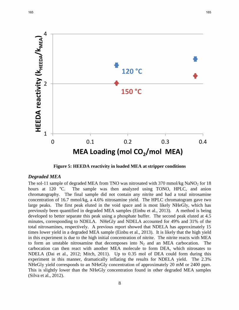
8

Figure 5: HEEDA reactivity in loaded MEA at stripper conditions

Degraded MEA

The sol-11 sample of degraded MEA from TNO was nitrosated with 370 mmol/kg NaNO2 for 18

hours at 120 °C. The sample was then analyzed using TONO, HPLC, and anion

chromatography. The final sample did not contain any nitrite and had a total nitrosamine

concentration of 16.7 mmol/kg, a 4.6% nitrosamine yield. The HPLC chromatogram gave two

large peaks. The first peak eluted in the void space and is most likely NHeGly, which has

previously been quantified in degraded MEA samples (Einbu et al., 2013). A method is being

developed to better separate this peak using a phosphate buffer. The second peak eluted at 4.5

minutes, corresponding to NDELA. NHeGly and NDELA accounted for 49% and 31% of the

total nitrosamines, respectively. A previous report showed that NDELA has approximately 15

times lower yield in a degraded MEA sample (Einbu et al., 2013). It is likely that the high yield

in this experiment is due to the high initial concentration of nitrite. The nitrite reacts with MEA

to form an unstable nitrosamine that decomposes into N2 and an MEA carbocation. The

carbocation can then react with another MEA molecule to form DEA, which nitrosates to

NDELA (Dai et al., 2012; Mitch, 2011). Up to 0.35 mol of DEA could form during this

experiment in this manner, dramatically inflating the results for NDELA yield. The 2.3%

NHeGly yield corresponds to an NHeGly concentration of approximately 20 mM or 2400 ppm.

This is slightly lower than the NHeGly concentration found in other degraded MEA samples

(Silva et al., 2012).

120 °C

150 °C

1

2

4

0 0.1 0.2 0.3 0.4

HEE

DA

re

acti

vity

(k H

EED

A/k

MEA

)

MEA Loading (mol CO2/mol MEA)

165 165

9

Pilot Plant Nitrosamines

Total nitrosamines were measured for samples from the PP2 PZ campaign and the Tarong PZ

campaign. TONO results matched previous HPLC results for MNPZ, so there are no other

significant nitrosamines in PZ. Degraded MEA samples from NCCC, SRP, and TNO were also

analyzed using TONO and contained 0.1–0.3 mmol/kg of total nitrosamine. The MEA samples

were also analyzed using anion chromatography and had appreciable amounts of nitrite. Since

nitrite is a known signal interference for TONO analysis, special care must be taken to either pre-

treat pilot plant samples with sulfamic acid or adjust TONO results to account for nitrite (Dai et

al., 2012; Kulshrestha et al., 2010). Pilot plant samples from TNO were analyzed on the HPLC,

but nitrosamine concentration was too low to detect in the degraded solution.

Conclusions

Nitrosamine formation is carbamate catalyzed.

Nitrosation kinetics decreases in the order: Secondary>Primary>>Tertiary/Hindered.

Very high nitrosamine yields can be expected in amine blends with secondary amines.

Nitrosamine yield in degraded primary amines is proportional to the secondary amine

concentration.

HeGly nitrosates 4.6 times faster than MEA under stripper conditions.

NHeGly yield has minor temperature and loading dependencies.

HEEDA nitrosates 2.8 times faster than MEA under stripper conditions.

HEEDA nitrosation has a minor loading dependency, but has an activation energy 6–13

kJ/mol less than MEA.

Degraded MEA from TNO had a 4.6% total nitrosamine yield when spiked with nitrite.

49% of the yield is from NHeGly, 31% is from NDELA, and <1% is from NHEEDA.

NDELA yield was most likely inflated by DEA formation during the experiment.

Future Work

Develop amino acid HPLC analysis for HeGly.

Develop better HPLC analysis of NHeGly.

Measure thermal decomposition rates of NHeGly.

Determine NO2 absorption rates and products.

Determine nitrosamine volatility under thermal reclaimer conditions.

Find final products from MNPZ decomposition.

References

Closmann FB. Oxidation and thermal degradation of methyldiethanolamine/piperazine in CO2

capture. The University of Texas at Austin. Ph.D. Dissertation. 2011.

Dai N, Shah AD, Hu L, Plewa MJ, Mckague B, Mitch WA. "Measurement of Nitrosamine and

Nitramine Formation from NOx Reactions with Amines during Amine-Based Carbon

Dioxide Capture for Postcombustion Carbon Sequestration." Environ Sci Technol.

2007;46:9793–9801.

166 166

10

Dugas, RE. Carbon dioxide absorption, desorption, and diffusion in aqueous piperazine and

monoethanolamine. The University of Texas at Austin. Ph.D. Dissertation. 2009.

Einbu A, DaSilva E, Haugen G, Grimstvedt A, Lauritsen KG, Zahlsen K, Vassbotn T. "A new

test rig for studies of degradation of CO2 absorption solvents at process conditions;

comparison of test rig results and pilot plant data for degradation of MEA" Presented at

GHGT-11, Kyoto, Japan, November 18-22, 2012. Energy Proc. 2013.

Kulshrestha P, McKinstry KC, Fernandez BO, Feelisch M, Mitch WA. "Application of an

optimized total N-nitrosamine (TONO) assay to pools: placing N-nitrosodimethylamine

(NDMA) determinations into perspective." Environ Sci Technol. 2010;45(9):3369–75.

doi:10.1021/es100361f.

Mitch W. Critical Literature Review of Nitrosation/Nitration Pathways. Gassnova. Retrieved

from http://www.gassnova.no/frontend/files/CONTENT/Rapporter/Nitrosamine

andNitramineformationchemistry_YALE.pdf. accessed on November 2011.

DaSilva E, Grimstvedt A, Vevelstad SJ, Einbu A, Vernstad K, Svendsen HF, Zahlsen K.

"Understanding 2 - Ethanolamine Degradation in Postcombustion CO2 Capture." Ind Eng

Chem Res. 2012;51:13329−13338.

167 167

11

Appendix A

Figure 6: High Resolution Mass Spectroscopy of HeGly/NHeGly in MEA

Figure 7: HeGly peak in High Resolution Mass Spectroscopy of HeGly/NHeGly in MEA

NHeGly HeGly

HeGly

Acceptable Error

in Mass

168 168

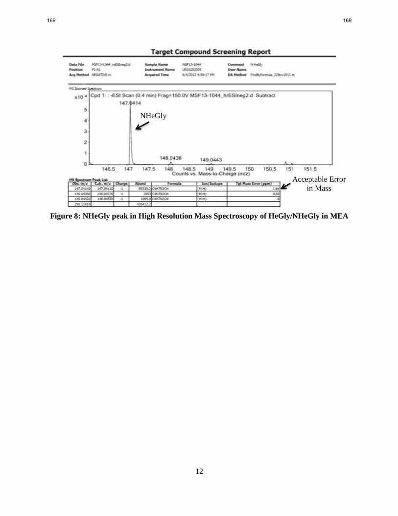
12

Figure 8: NHeGly peak in High Resolution Mass Spectroscopy of HeGly/NHeGly in MEA

NHeGly

Acceptable Error

in Mass

169 169

13

Appendix B

Figure 9: NHeGly Calibration from TONO results

Figure 10: NHeGly elution, no nitrite present

y = 0.0199x + 0.0016 R² = 1.0000

0.001

0.010

0.100

1.000

0.1 1.0 10.0

NH

eG

ly f

rom

TO

NO

(m

mo

l/kg

)

NHeGly Peak Area from HPLC

0.0

0.5

1.0

1.5

2.0

2.5

3.0

0 2 4 6 8 10

Ab

sorb

ance

(m

Au

)

Elution Time (Minutes)

HeGly

170 170

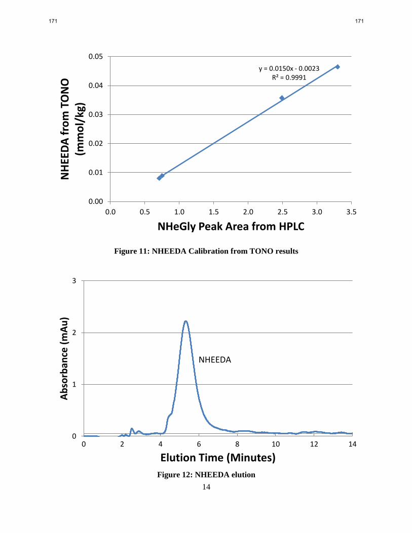
14

Figure 11: NHEEDA Calibration from TONO results

Figure 12: NHEEDA elution

y = 0.0150x - 0.0023 R² = 0.9991

0.00

0.01

0.02

0.03

0.04

0.05

0.0 0.5 1.0 1.5 2.0 2.5 3.0 3.5

NH

EED

A f

rom

TO

NO

(m

mo

l/kg

)

NHeGly Peak Area from HPLC

0

1

2

3

0 2 4 6 8 10 12 14

Ab

sorb

ance

(m

Au

)

Elution Time (Minutes)

NHEEDA

171 171

co2 capture by aqueous absorption - university of texas at...

Documents