CMSC 671CMSC 671Fall 2005Fall 2005

Class #5 – Thursday, September 15

Today’s class

• Heuristic search• Best-first search

– Greedy search– Beam search– A, A*– Examples

• Memory-conserving variations of A*• Heuristic functions• Iterative improvement methods

– Hill climbing– Simulated annealing– Local beam search– Genetic algorithms

• Online search

InformedInformedSearchSearchChapter 4Chapter 4

Some material adopted from notes by Charles R. Dyer, University of

Wisconsin-Madison

Note: We will skip Section 4.4

Heuristic

Webster's Revised Unabridged Dictionary (1913) (web1913)

Heuristic \Heu*ris"tic\, a. [Gr. ? to discover.] Serving to discover or find out.

The Free On-line Dictionary of Computing (15Feb98)

heuristic 1. <programming> A rule of thumb, simplification or educated guess that reduces or limits the search for solutions in domains that are difficult and poorly understood. Unlike algorithms, heuristics do not guarantee feasible solutions and are often used with no theoretical guarantee. 2. <algorithm> approximation algorithm.

From WordNet (r) 1.6 heuristic adj 1: (computer science) relating to or using a heuristic rule 2:

of or relating to a general formulation that serves to guide investigation [ant: algorithmic] n : a commonsense rule (or set of rules) intended to increase the probability of solving some problem [syn: heuristic rule, heuristic program]

Informed methods add domain-specific information

• Add domain-specific information to select the best path along which to continue searching

• Define a heuristic function, h(n), that estimates the “goodness” of a node n.

• Specifically, h(n) = estimated cost (or distance) of minimal cost path from n to a goal state.

• The heuristic function is an estimate, based on domain-specific information that is computable from the current state description, of how close we are to a goal

Heuristics• All domain knowledge used in the search is encoded in the

heuristic function h.

• Heuristic search is an example of a “weak method” because of the limited way that domain-specific information is used to solve the problem.

• Examples:– Missionaries and Cannibals: Number of people on starting river bank

– 8-puzzle: Number of tiles out of place

– 8-puzzle: Sum of distances each tile is from its goal position

• In general:– h(n) >= 0 for all nodes n

– h(n) = 0 implies that n is a goal node

– h(n) = infinity implies that n is a dead-end from which a goal cannot be reached

Weak vs. strong methods• We use the term weak methods to refer to methods that are

extremely general and not tailored to a specific situation.

• Examples of weak methods include – Means-ends analysis is a strategy in which we try to represent the

current situation and where we want to end up and then look for ways to shrink the differences between the two.

– Space splitting is a strategy in which we try to list the possible solutions to a problem and then try to rule out classes of these possibilities.

– Subgoaling means to split a large problem into several smaller ones that can be solved one at a time.

• Called “weak” methods because they do not take advantage of more powerful domain-specific heuristics

Best-first search

• Order nodes on the nodes list by increasing value of an evaluation function, f(n), that incorporates domain-specific information in some way.

• This is a generic way of referring to the class of informed methods.

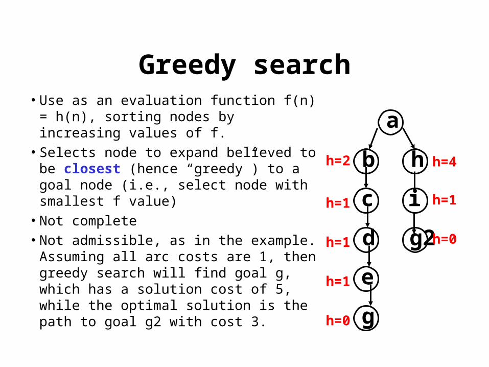
Greedy search• Use as an evaluation function f(n) = h(n),

sorting nodes by increasing values of f.

• Selects node to expand believed to be closest (hence “greedy”) to a goal node (i.e., select node with smallest f value)

• Not complete

• Not admissible, as in the example. Assuming all arc costs are 1, then greedy search will find goal g, which has a solution cost of 5, while the optimal solution is the path to goal g2 with cost 3.

a

hb

c

d

e

g

i

g2

h=2

h=1

h=1

h=1

h=0

h=4

h=1

h=0

Beam search

• Use an evaluation function f(n) = h(n), but the maximum size of the nodes list is k, a fixed constant

• Only keeps k best nodes as candidates for expansion, and throws the rest away

• More space efficient than greedy search, but may throw away a node that is on a solution path

• Not complete

• Not admissible

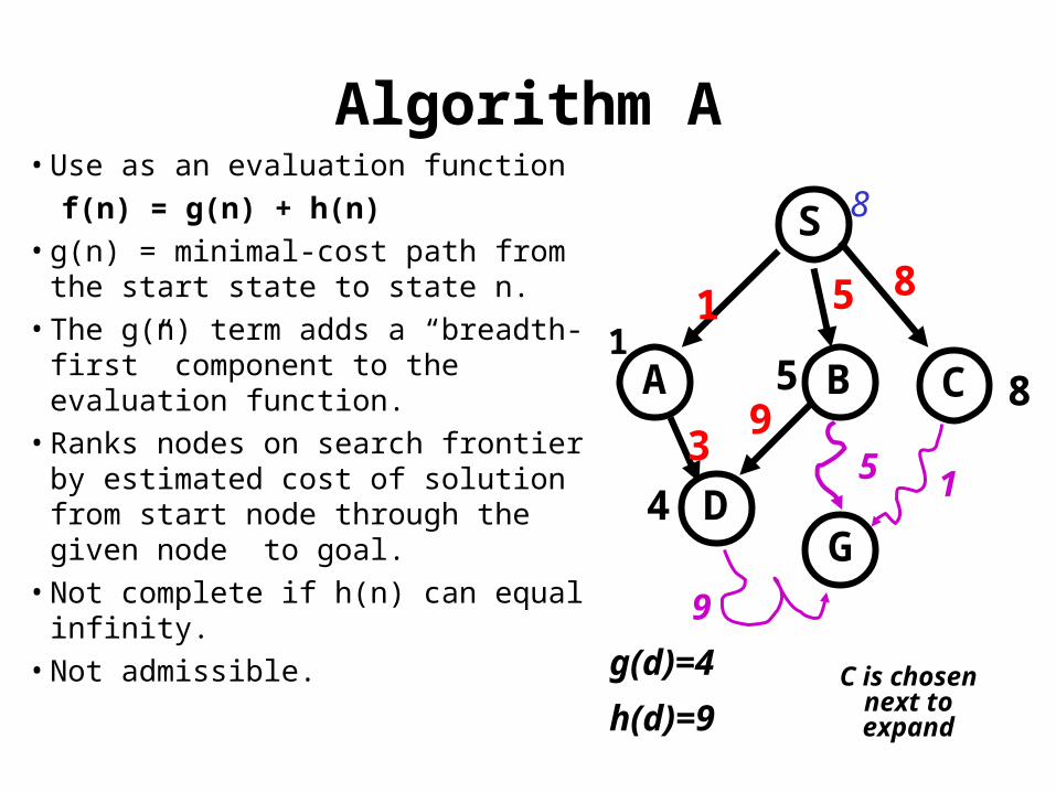
Algorithm A• Use as an evaluation function

f(n) = g(n) + h(n)

• g(n) = minimal-cost path from the start state to state n.

• The g(n) term adds a “breadth-first” component to the evaluation function.

• Ranks nodes on search frontier by estimated cost of solution from start node through the given node to goal.

• Not complete if h(n) can equal infinity.

• Not admissible.

S

BA

DG

1 5 8

3

8

1

5

C

1

9

4

5 89

g(d)=4

h(d)=9C is chosen

next to expand

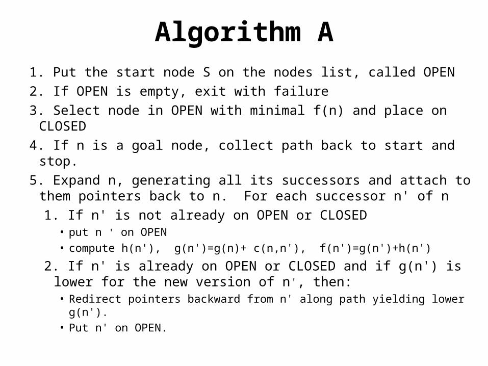
Algorithm A

1. Put the start node S on the nodes list, called OPEN

2. If OPEN is empty, exit with failure

3. Select node in OPEN with minimal f(n) and place on CLOSED

4. If n is a goal node, collect path back to start and stop.

5. Expand n, generating all its successors and attach to them pointers back to n. For each successor n' of n

1. If n' is not already on OPEN or CLOSED• put n ' on OPEN

• compute h(n'), g(n')=g(n)+ c(n,n'), f(n')=g(n')+h(n')

2. If n' is already on OPEN or CLOSED and if g(n') is lower for the new version of n', then:• Redirect pointers backward from n' along path yielding lower g(n').• Put n' on OPEN.

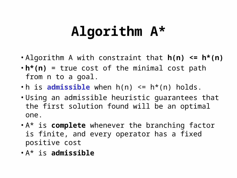
Algorithm A*

• Algorithm A with constraint that h(n) <= h*(n)

• h*(n) = true cost of the minimal cost path from n to a goal.

• h is admissible when h(n) <= h*(n) holds.

• Using an admissible heuristic guarantees that the first solution found will be an optimal one.

• A* is complete whenever the branching factor is finite, and every operator has a fixed positive cost

• A* is admissible

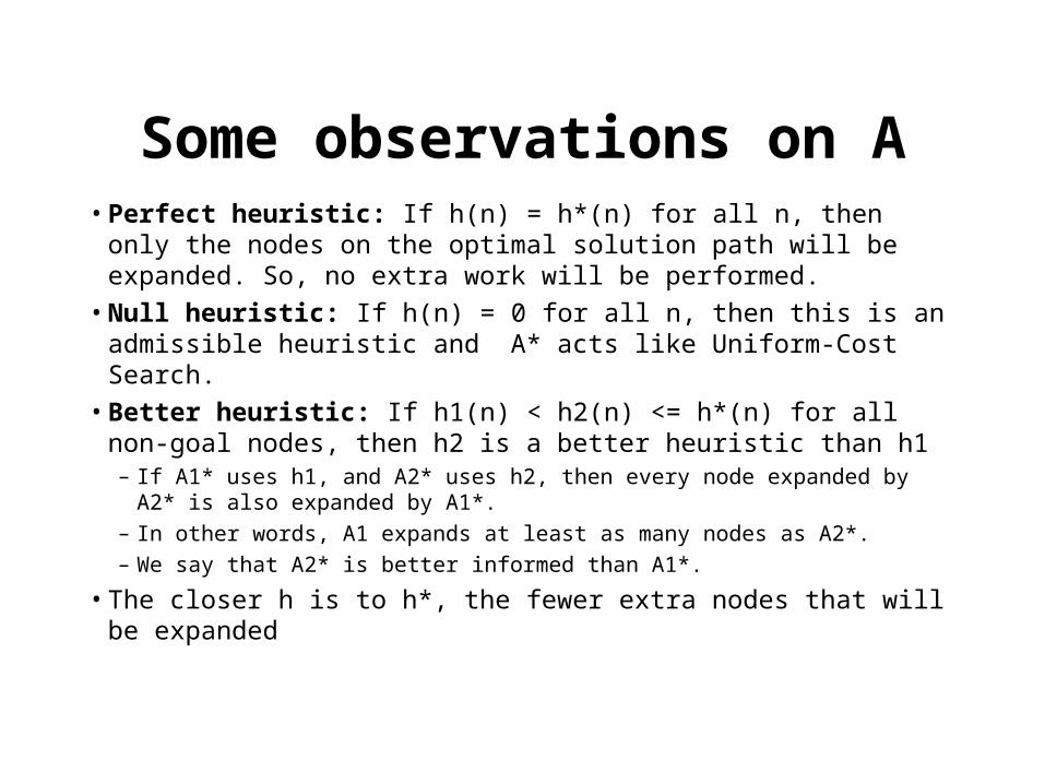
Some observations on A• Perfect heuristic: If h(n) = h*(n) for all n, then only the nodes on

the optimal solution path will be expanded. So, no extra work will be performed.

• Null heuristic: If h(n) = 0 for all n, then this is an admissible heuristic and A* acts like Uniform-Cost Search.

• Better heuristic: If h1(n) < h2(n) <= h*(n) for all non-goal nodes, then h2 is a better heuristic than h1 – If A1* uses h1, and A2* uses h2, then every node expanded by A2* is also

expanded by A1*. – In other words, A1 expands at least as many nodes as A2*. – We say that A2* is better informed than A1*.

• The closer h is to h*, the fewer extra nodes that will be expanded

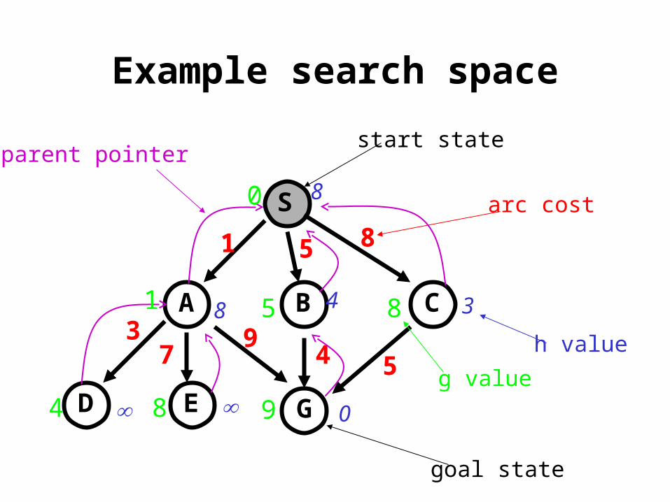
Example search space

S

CBA

D GE

1 5 8

94 5

37

8

8 4 3

0

start state

goal state

arc cost

h value

parent pointer

0

1

4 8 9

85

g value

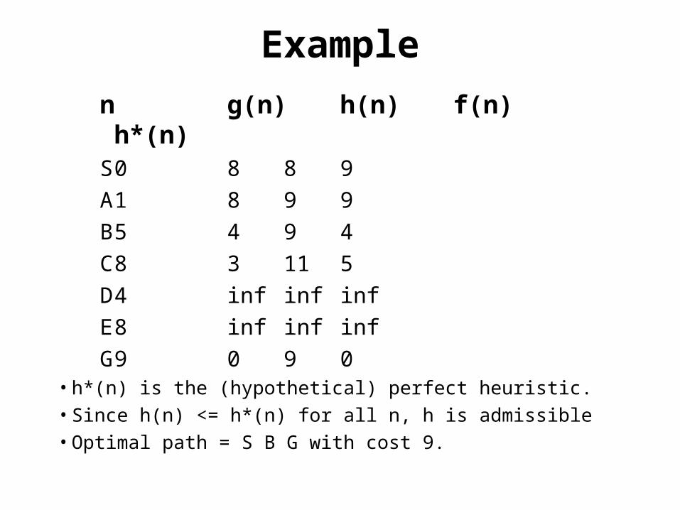
Example

n g(n) h(n) f(n) h*(n)S 0 8 8 9

A 1 8 9 9

B 5 4 9 4

C 8 3 11 5

D 4 inf inf inf

E 8 inf inf inf

G 9 0 9 0• h*(n) is the (hypothetical) perfect heuristic.• Since h(n) <= h*(n) for all n, h is admissible• Optimal path = S B G with cost 9.

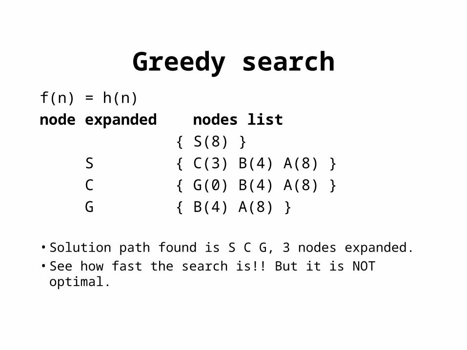
Greedy searchf(n) = h(n)

node expanded nodes list { S(8) } S { C(3) B(4) A(8) } C { G(0) B(4) A(8) } G { B(4) A(8) }

• Solution path found is S C G, 3 nodes expanded. • See how fast the search is!! But it is NOT optimal.

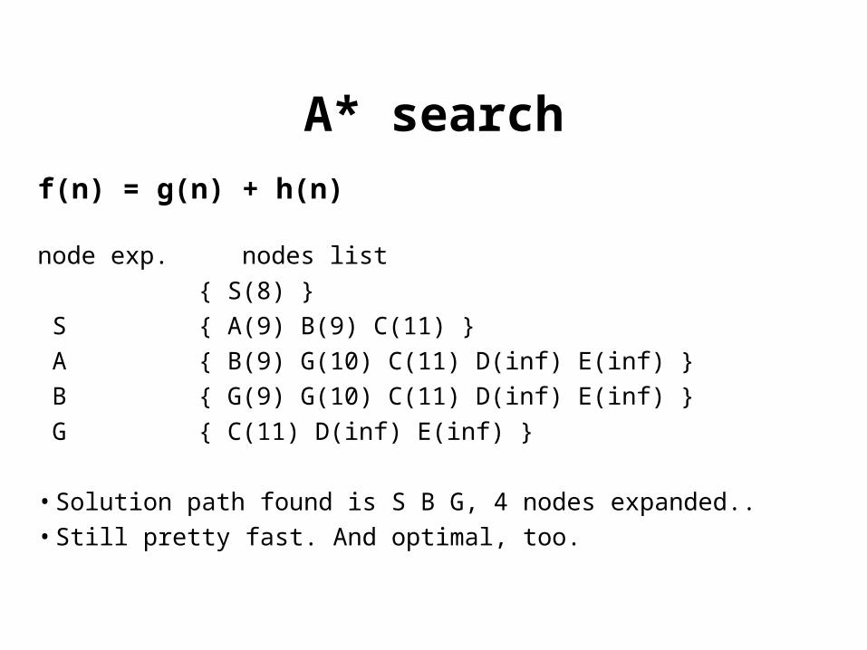
A* search

f(n) = g(n) + h(n)

node exp. nodes list { S(8) } S { A(9) B(9) C(11) } A { B(9) G(10) C(11) D(inf) E(inf) } B { G(9) G(10) C(11) D(inf) E(inf) } G { C(11) D(inf) E(inf) }

• Solution path found is S B G, 4 nodes expanded..

• Still pretty fast. And optimal, too.

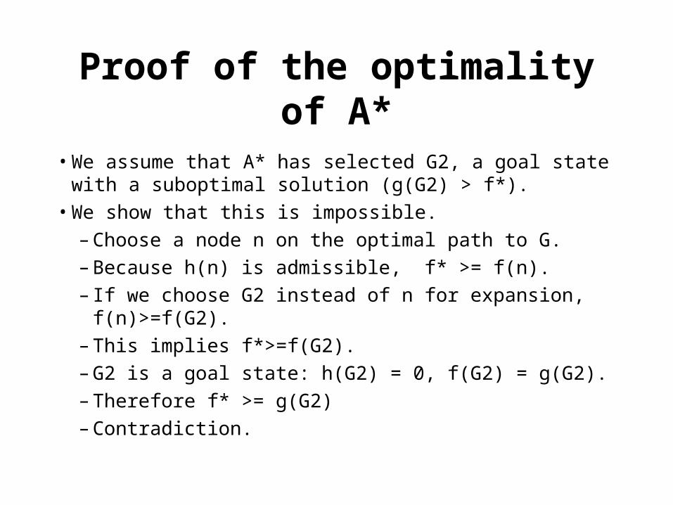
Proof of the optimality of A*

• We assume that A* has selected G2, a goal state with a suboptimal solution (g(G2) > f*).

• We show that this is impossible.

– Choose a node n on the optimal path to G.

– Because h(n) is admissible, f* >= f(n).

– If we choose G2 instead of n for expansion, f(n)>=f(G2).

– This implies f*>=f(G2).

– G2 is a goal state: h(G2) = 0, f(G2) = g(G2).

– Therefore f* >= g(G2)

– Contradiction.

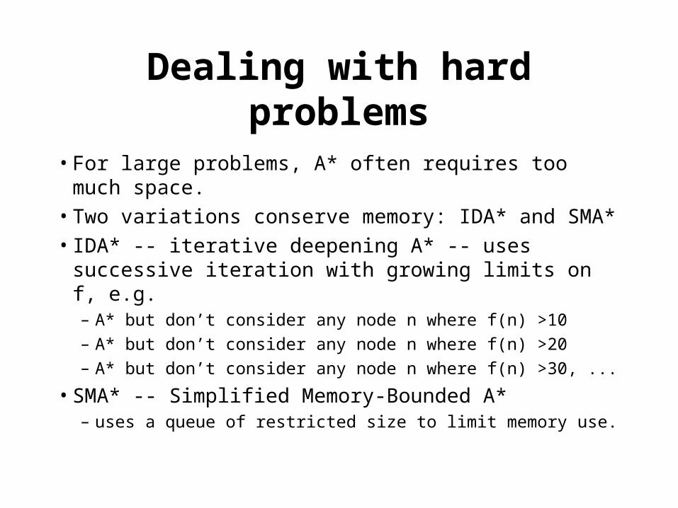
Dealing with hard problems

• For large problems, A* often requires too much space.

• Two variations conserve memory: IDA* and SMA*

• IDA* -- iterative deepening A* -- uses successive iteration with growing limits on f, e.g.– A* but don’t consider any node n where f(n) >10

– A* but don’t consider any node n where f(n) >20

– A* but don’t consider any node n where f(n) >30, ...

• SMA* -- Simplified Memory-Bounded A*– uses a queue of restricted size to limit memory use.

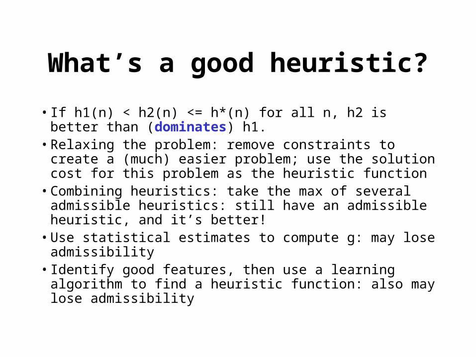
What’s a good heuristic?

• If h1(n) < h2(n) <= h*(n) for all n, h2 is better than (dominates) h1.

• Relaxing the problem: remove constraints to create a (much) easier problem; use the solution cost for this problem as the heuristic function

• Combining heuristics: take the max of several admissible heuristics: still have an admissible heuristic, and it’s better!

• Use statistical estimates to compute g: may lose admissibility

• Identify good features, then use a learning algorithm to find a heuristic function: also may lose admissibility

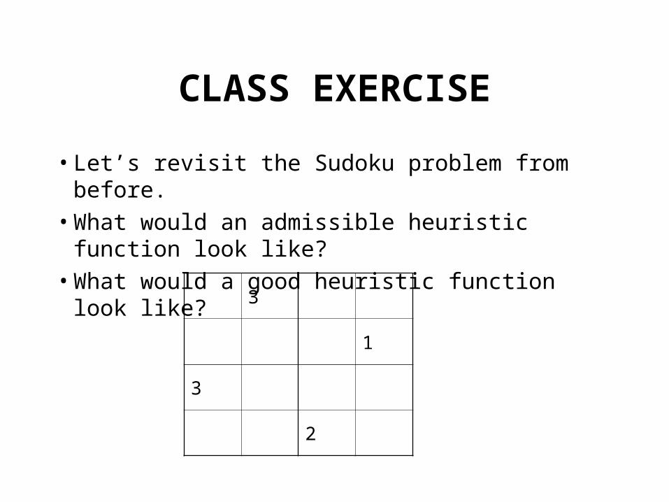
CLASS EXERCISE

• Let’s revisit the Sudoku problem from before.

• What would an admissible heuristic function look like?

• What would a good heuristic function look like?

3

1

3

2

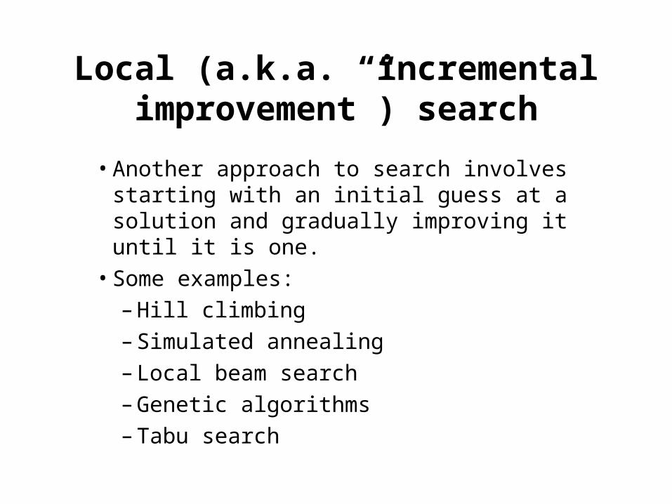
Local (a.k.a. “incremental improvement”) search

• Another approach to search involves starting with an initial guess at a solution and gradually improving it until it is one.

• Some examples:

– Hill climbing

– Simulated annealing

– Local beam search

– Genetic algorithms

– Tabu search

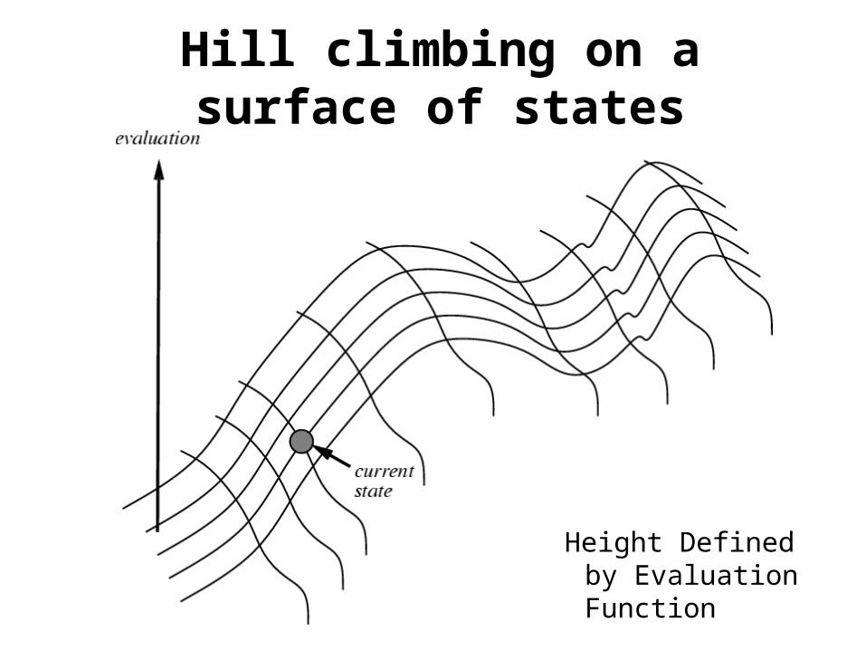
Hill climbing on a surface of states

Height Defined by Evaluation Function

Hill-climbing search• If there exists a successor s for the current state n such that

– h(s) < h(n)

– h(s) <= h(t) for all the successors t of n,

• then move from n to s. Otherwise, halt at n.

• Looks one step ahead to determine if any successor is better than the current state; if there is, move to the best successor.

• Similar to Greedy search in that it uses h, but does not allow backtracking or jumping to an alternative path since it doesn’t “remember” where it has been.

• Corresponds to Beam search with a beam width of 1 (i.e., the maximum size of the nodes list is 1).

• Not complete since the search will terminate at "local minima," "plateaus," and "ridges."

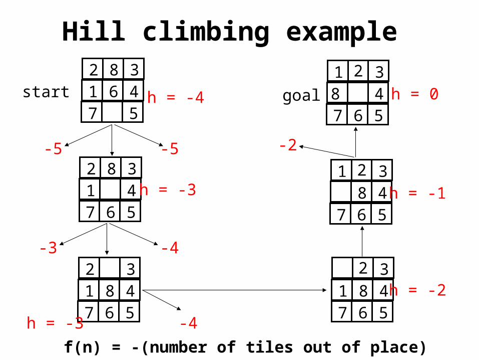
Hill climbing example 2 8 31 6 47 5

2 8 31 47 6 5

2 31 8 47 6 5

1 3 8 47 6 5

2

31 8 47 6 5

2

1 38 47 6 5

2start goal

-5

h = -3

h = -3

h = -2

h = -1

h = 0h = -4

-5

-4

-4-3

-2

f(n) = -(number of tiles out of place)

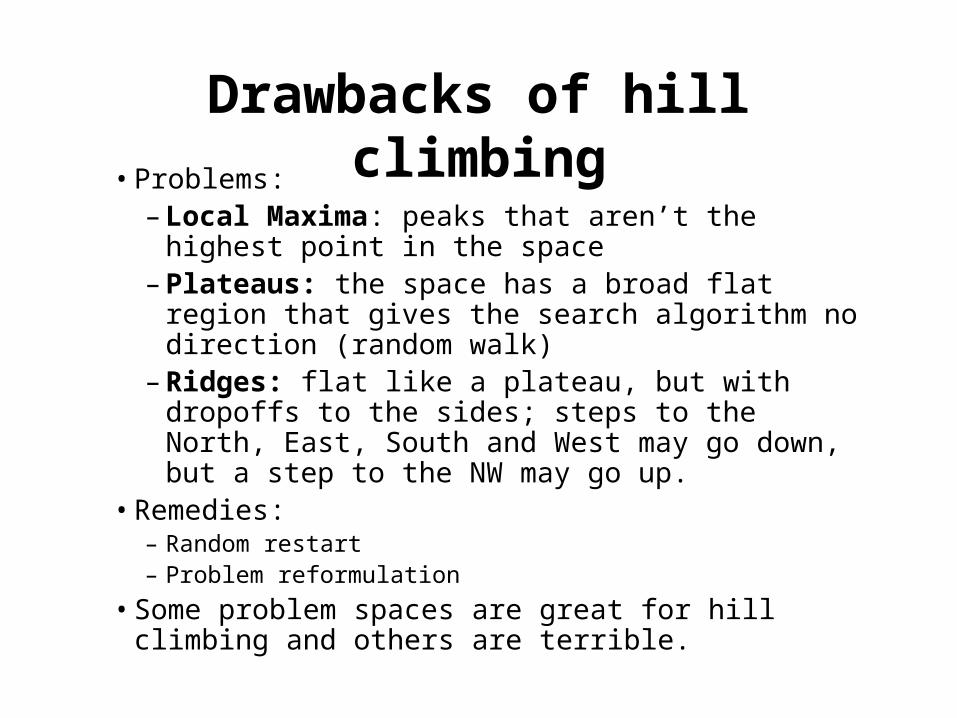
Drawbacks of hill climbing• Problems:

– Local Maxima: peaks that aren’t the highest point in the space

– Plateaus: the space has a broad flat region that gives the search algorithm no direction (random walk)

– Ridges: flat like a plateau, but with dropoffs to the sides; steps to the North, East, South and West may go down, but a step to the NW may go up.

• Remedies: – Random restart– Problem reformulation

• Some problem spaces are great for hill climbing and others are terrible.

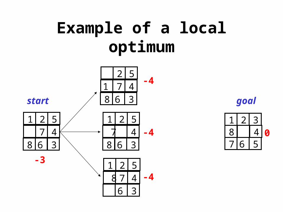
Example of a local optimum

1 2 5 7 48 6 3

41 2 387 6 5

1 2 5 7 48 6 3

2 51 7 48 6 3

1 2 5 8 7 4

6 3

-3

-4

-4

-4

0

start goal

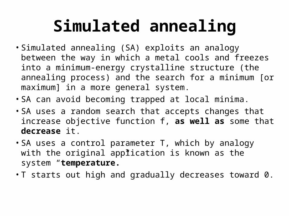
Simulated annealing• Simulated annealing (SA) exploits an analogy between the way

in which a metal cools and freezes into a minimum-energy crystalline structure (the annealing process) and the search for a minimum [or maximum] in a more general system.

• SA can avoid becoming trapped at local minima.

• SA uses a random search that accepts changes that increase objective function f, as well as some that decrease it.

• SA uses a control parameter T, which by analogy with the original application is known as the system “temperature.”

• T starts out high and gradually decreases toward 0.

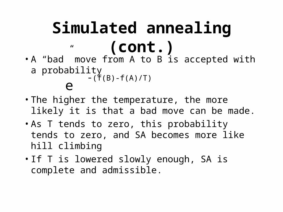
Simulated annealing (cont.)• A “bad” move from A to B is accepted with a probability

-(f(B)-f(A)/T)e

• The higher the temperature, the more likely it is that a bad move can be made.

• As T tends to zero, this probability tends to zero, and SA becomes more like hill climbing

• If T is lowered slowly enough, SA is complete and admissible.

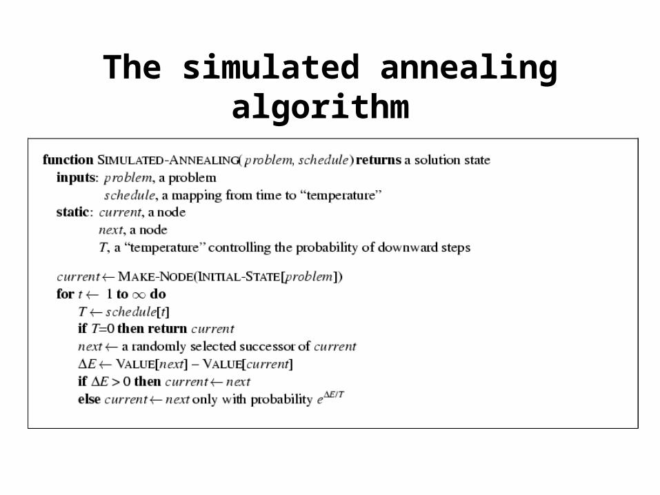
The simulated annealing algorithm

Local beam search

• Begin with k random states

• Generate all successors of these states

• Keep the k best states

• Stochastic beam search: Probability of keeping a state is a function of its heuristic value

Genetic algorithms

• Similar to stochastic beam search

• Start with k random states (the initial population)

• New states are generated by “mutating” a single state or “reproducing” (combining) two parent states (selected according to their fitness)

• Encoding used for the “genome” of an individual strongly affects the behavior of the search

• Genetic algorithms / genetic programming are a large and active area of research

Tabu search

• Problem: Hill climbing can get stuck on local maxima

• Solution: Maintain a list of k previously visited states, and prevent the search from revisiting them

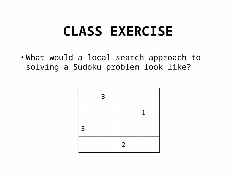
CLASS EXERCISE

• What would a local search approach to solving a Sudoku problem look like?

3

1

3

2

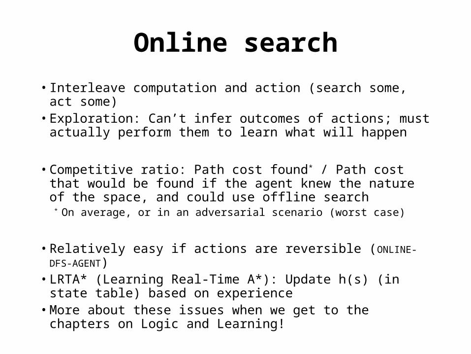
Online search

• Interleave computation and action (search some, act some)• Exploration: Can’t infer outcomes of actions; must actually

perform them to learn what will happen

• Competitive ratio: Path cost found* / Path cost that would be found if the agent knew the nature of the space, and could use offline search

* On average, or in an adversarial scenario (worst case)

• Relatively easy if actions are reversible (ONLINE-DFS-AGENT)• LRTA* (Learning Real-Time A*): Update h(s) (in state

table) based on experience• More about these issues when we get to the chapters on

Logic and Learning!

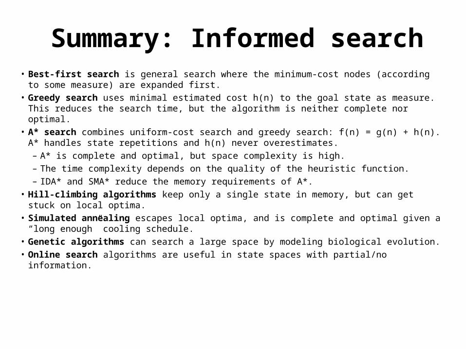
Summary: Informed search• Best-first search is general search where the minimum-cost nodes (according to some

measure) are expanded first. • Greedy search uses minimal estimated cost h(n) to the goal state as measure. This reduces the

search time, but the algorithm is neither complete nor optimal. • A* search combines uniform-cost search and greedy search: f(n) = g(n) + h(n). A* handles

state repetitions and h(n) never overestimates. – A* is complete and optimal, but space complexity is high.– The time complexity depends on the quality of the heuristic function. – IDA* and SMA* reduce the memory requirements of A*.

• Hill-climbing algorithms keep only a single state in memory, but can get stuck on local optima.

• Simulated annealing escapes local optima, and is complete and optimal given a “long enough” cooling schedule.

• Genetic algorithms can search a large space by modeling biological evolution.• Online search algorithms are useful in state spaces with partial/no information.