cmmm 1895764 1

Research ArticleStability and Hopf Bifurcation Analysis of an Epidemic Model withTime Delay

Yue Zhang ,1 Xue Li ,2 Xianghua Zhang ,3 and Guisheng Yin 1

1College of Computer Science and Technology, Harbin Engineering University, Harbin 150001, China2School of Computer Science and Technology, Harbin Institute of Technology, Harbin 150001, China3College of Science, Heilongjiang University of Science and Technology, China

Correspondence should be addressed to Yue Zhang; [email protected]

Received 3 May 2021; Accepted 10 June 2021; Published 2 July 2021

Academic Editor: Lei Chen

Copyright © 2021 Yue Zhang et al. This is an open access article distributed under the Creative Commons Attribution License,which permits unrestricted use, distribution, and reproduction in any medium, provided the original work is properly cited.

Epidemic models are normally used to describe the spread of infectious diseases. In this paper, we will discuss an epidemic modelwith time delay. Firstly, the existence of the positive fixed point is proven; and then, the stability and Hopf bifurcation areinvestigated by analyzing the distribution of the roots of the associated characteristic equations. Thirdly, the theory of normalform and manifold is used to drive an explicit algorithm for determining the direction of Hopf bifurcation and the stability ofthe bifurcation periodic solutions. Finally, some simulation results are carried out to validate our theoretic analysis.

1. Introduction

Today, the serious epidemics, such as SARS and H1N1, arestill threatening the life of people continually. Plenty of math-ematical models have been proposed to analyze the spreadand the control of these diseases [1–7].

However, many infectious diseases, for instance, gonor-rhea and syphilis, occur and spread amongst the mature,while some epidemics, for example, chickenpox and FMD,only result in infection and death in immature. For this rea-son, stage structure should be taken into consideration inmodels. Aliello and Freedman [8] proposed a stage-structured model described by

_x tð Þ = αy tð Þ − γx tð Þ − αe−γτy t − τð Þ_y tð Þ = αe−γτy t − τð Þ − βy2 tð Þ

(, ð1Þ

where xðtÞ is the immature population density and yðtÞrepresents the density of the mature population. α, γ, τ, andβ are all positive constants. α is the birth rate, and γ is thenatural death rate; τ is the time from birth to maturity; β isthe death rate of the mature because of the competition witheach other.

And then, many infectious diseases with sage structurehave been built and investigated [9–14]. Xiao and Chen[15] improved (1) by separating the population into matureand immature and supposing that only the immature weresusceptible to the infection.

Based on the model in [15], supposing that only themature were susceptible, Jia and Li [16] built a new oneas follows:

_x tð Þ = αe−γτx t − τð Þ − γx tð Þ − βx2 tð Þ −mx tð Þy tð Þ_y tð Þ =mx tð Þy tð Þ − γy tð Þ − cy tð Þ − gy tð Þ_z tð Þ = αx tð Þ − γz tð Þ − αe−γτx t − τð Þ_R tð Þ = gy tð Þ − γR tð Þ

8>>>>><>>>>>:

,

ð2Þ

where xðtÞ, yðtÞ, and RðtÞ are the susceptible, infec-tious, and recovered mature population densities, respec-tively; zðtÞ denotes the immature population density. Allthe parameters are positive constants. α, β, γ, and τ arethe same as those in (1); m is the transmission coefficientdescribing the infection between the susceptible and theinfectious; c is the death rate because of the epidemic; g

HindawiComputational and Mathematical Methods in MedicineVolume 2021, Article ID 1895764, 15 pageshttps://doi.org/10.1155/2021/1895764

https://orcid.org/0000-0002-4515-8931

https://orcid.org/0000-0001-5885-0794

https://orcid.org/0000-0002-8824-3538

https://orcid.org/0000-0003-0924-4741

https://creativecommons.org/licenses/by/4.0/

https://doi.org/10.1155/2021/1895764

is the recovery rate; αe−γτxðt − τÞ denotes the populationwho were born at t − τ and survive at t.

In systems (1) and (2), the time delay was also taken intoconsideration. Indeed, time delay plays an important role inthe epidemic system, making the models more accurate. Inrecent years, delays have been introduced in more and moreepidemic and predator-prey systems [17–19].

In this paper, on the basis of (2), we further assume that

(1) Both the susceptible and the infectious have fertility,while in (2), only the susceptible is fertile

(2) For the infectious, there is competition with all thesusceptible and the infectious, while for the suscepti-ble, there is only competition between generations

Meanwhile, all the death of the susceptible, the same asthat in (1), is only due to the competition. To simplify model(2), we denote γ + c + g = d, and let bðxðtÞ + yðtÞÞ present thetransmission from immature to mature.

As a consequence, the new epidemic model could bedescribed as follows:

_x tð Þ = b x tð Þ + y tð Þð Þ −w x t − τð Þ + y t − τð Þð Þx tð Þ −mx tð Þy tð Þ_y tð Þ =mx tð Þy tð Þ −w x tð Þ + y tð Þð Þy tð Þ − dy tð Þ_z tð Þ = α x tð Þ + y tð Þð Þ − γz tð Þ − b x tð Þ + y tð Þð Þ_R tð Þ = gy tð Þ − γR tð Þ

8>>>>><>>>>>:

,

ð3Þ

where w is the death rate of the mature because of thecompetition.

We can notice that zðtÞ depends on xðtÞ and yðtÞ and RðtÞ depends on yðtÞ; however, xðtÞ and yðtÞ have nothing todo with zðtÞ and RðtÞ. According to Qu andWei [20], we willmainly focus on xðtÞ and yðtÞ, that is,

_x tð Þ = b x tð Þ + y tð Þð Þ −w x t − τð Þ + y t − τð Þð Þx tð Þ −mx tð Þy tð Þ_y tð Þ =mx tð Þy tð Þ −w x tð Þ + y tð Þð Þy tð Þ − dy tð Þ

:

(

ð4Þ

The rest of the paper is organized as follows. In Section 2,we calculate the steady states of system (4) and prove theexistence and uniqueness of the positive equilibrium in par-ticular. And then, the stability of the two nonzero equilibriaand the existence of the Hopf bifurcation are investigated inSections 3 and 4, respectively. In Section 5, the directionand stability of the Hopf bifurcation at the positive equilib-rium are studied by using the center manifold theorem andthe normal form theory [21]. And in the last section, somenumerical simulations are carried out to validate the theoret-ical analysis.

2. The Existence and Uniqueness of the PositiveEquilibrium of the Model

In this section, we discuss the existence of the equilibria of (4)and the positive one in particular.

The equilibria are the solutions of the equations (5),

b x + yð Þ −w x + yð Þx −mxy = 0mx −w x + yð Þ − d½ �y = 0

(: ð5Þ

Clearly, E1ð0, 0Þ and E2ðb/w, 0Þ are two equilibria of (4).In the following, we will focus on the existence of the pos-

itive equilibrium.

Theorem 1. If bðm −wÞ > dw, (4) has one positive equilib-rium E3ðx∗, y∗Þ, where

x∗ = B +ffiffiffiffiΔ

p� �2m2� �

, y∗ = m −wð Þ B +ffiffiffiffiΔ

p� �/ 2m2w� �

− d/w:

ð6Þ

Proof. Positive equilibrium is the positive solution of theequations (7),

b x + yð Þ −w x + yð Þx −mxy = 0mx −w x + yð Þ − d = 0

(: ð7Þ

From the second equation of (7), we have

wy = m −wð Þx − d: ð8Þ

Taking (8) into the first equation of (7), we can obtain

m2x2 − bm + dm + dwð Þx + bd = 0, ð9Þ

which leads to

Δ = B2 − 4m2bd = bm + dw − dmð Þ2 + 4d2mw > 0, ð10Þ

where

B = bm + dm + dw: ð11Þ

Together with

x1 + x2 = bm + dm + dwð Þ/m2 > 0, and x1x2 = bd/m2 > 0,ð12Þ

we can know that both of the two solutions of (9) arepositive,

where

x1 =B −

ffiffiffiffiΔ

p

2m2 > 0andx2 =B +

ffiffiffiffiΔ

p

2m2 > 0: ð13Þ

If x = B −ffiffiffiffiΔ

p/2m2,

2 Computational and Mathematical Methods in Medicine

then,

wy = m −wð Þx − d

= m −wð ÞB −

ffiffiffiffiΔ

p� �2m2 − d

< m −wð Þ B − bm + dw − dmj j2m2 − d

≤ m −wð Þ B − bm + dw − dmð Þ2m2 − d

= −dwm

< 0:

ð14Þ

So, x = B −ffiffiffiffiΔ

p/2m2 is dropped.

If x = B +ffiffiffiffiΔ

p/2m2,

then,

wy = m −wð Þ B +ffiffiffiffiΔ

p

2m2 − d

= m −wð Þ 4m2bd

2m2 B −ffiffiffiffiΔ

p� � − d

= d2b m −wð ÞB −

ffiffiffiffiΔ

p − 1� �

= d B −ffiffiffiffiΔ

p� �2b m −wð Þ − B −

ffiffiffiffiΔ

p� �h i:

ð15Þ

w > 0, d > 0, and B −ffiffiffiffiΔ

p=

ffiffiffiffiffiffiffiffiffiffiffiffiffiffiffiffiffiffiffiΔ+4m2bd

p−

ffiffiffiffiΔ

p> 0, so

y > 0⟺ 2bðm −wÞ − ðB −ffiffiffiffiΔ

p Þ > 0,

⟺Δ > B2 − 4b m −wð ÞB + 4b2 m −wð Þ2 ⟺m2d

− m −wð Þ bm − bw − bm − dm − dwð Þ< 0⟺ b m −wð Þ > dw∴b m −wð Þ > dw⟺ y > 0:

ð16Þ

Then, taking x = B +ffiffiffiffiΔ

p/2m2 ≜ x∗ into (8), we have

y =m −wð Þ B +

ffiffiffiffiΔ

p� �2m2wð Þ −

dw

≜ y∗: ð17Þ

Therefore, if bðm −wÞ > dw, (4) has the unique pos-itive equilibrium E3ðx∗, y∗Þ. ☐

3. Stability Analysis of theEquilibrium E2ðb/w, 0Þ

In this section, we analyze the stability of the equilibriumE2ðb/w, 0Þ.

For convenience, the new variables uðtÞ = xðtÞ − b/w andvðtÞ = yðtÞ are introduced, and then, around E2ðb/w, 0Þ, thesystem (4) could be linearized as (18):

_u tð Þ = −bu t − τð Þ − bv t − τð Þ + bv tð Þ − bmw

v tð Þ

_v tð Þ = bmw

v tð Þ − dv tð Þ − bv tð Þ

8>><>>: , ð18Þ

whose characteristic equation is given by

λ + be−λτ� �

λ + b + d −bmw

= 0, ð19Þ

from which, we can get that

λ = − b + d −bmw

, ð20Þ

or

λ + be−λτ = 0: ð21Þ

Obviously, if bðm −wÞ > dw,then

λ = − b + d −bmw

> 0, ð22Þ

which implies that the equilibrium E2 is unstable.If bðm −wÞ < dw,then

λ = − b + d − bm/wð Þ < 0: ð23Þ

As a consequence, we will discuss the other roots of (19),that is, the roots of (21), under the condition bðm −wÞ < dw.

For τ = 0, equation (21) becomes

λ + b = 0, ð24Þ

whose root is

λ = −b < 0: ð25Þ

For τ > 0, if iωðω > 0Þ is a root of (21), then

iω + b cos ωτ − ib sin ωτ = 0: ð26Þ

(27) can be obtained by separating the real and the imag-inary parts,

b cos ωτ = 0b sin ωτ = ω

(, ð27Þ

which leads to

ω2 = b2, ð28Þ

3Computational and Mathematical Methods in Medicine

from which, we can get the unique positive root

ω0 = b: ð29Þ

Let

τj =π 4j + 1ð Þ

2ω0j = 0, 1, 2,⋯: ð30Þ

Then, when τ = τj, (21) has a pair of purely imaginaryroots ±iω0.

Suppose

λ τð Þ = α τð Þ + iω τð Þ, ð31Þ

which is the root of (21) such that

α τj� �

= 0, andω τj� �

= ω0: ð32Þ

To investigate the distribution of λðτÞ, we will discuss thetrend of λðτÞ at τ = τj.

Substituting λðτÞ into (21) and taking the derivative withrespect to τ, we can get

dλdτ

− be−λτ λ + τdλdτ

= 0, ð33Þ

which yields,

dλdτ

� �−1= eλτ

bλ−τ

λ: ð34Þ

Together with (27), we have

sign Re dλdτ

� �−1τ=τ j

( )= sign Re eλτ

bλ

� �τ=τ j

( )

= sign Re cos ω0τ + i sin ω0τ

ibω0

� ��

= sign sin ω0τ

bω0

� �= sign b sin ω0τ

b2ω0

� �

= sign ω0b2ω0

� �

= sign 1b2

� �> 0,

ð35Þ

which means that when undergoes τ = τj, λðτÞ will add apair of roots with positive real parts. That is, with the increaseof τ, the number of roots with positive real part is increasing,leading to the change of the stability of the system (4).

Therefore, the distribution of the roots of (21) could beobtained.

Lemma 2. Let ω0 and τj ( j = 0, 1, 2, ⋯ ) be defined by (29)and (30), respectively.

(1) If bðm −wÞ > dw, then (19) has at least one positiveroot

(2) If bðm −wÞ < dw, and τ = 0, then both roots of (19)are negative

(3) If bðm −wÞ < dw, and τ > 0, then (19) has a pair ofsimple imaginary roots ±iω0 at τ = τj; furthermore, ifτ < τ0, then all the roots of (19) have negative realparts; if τ ∈ ðτj, τj+1Þ, (19) has 2ðj + 1Þ roots with pos-itive real parts

Together with condition (35), the Hopf bifurcation theo-rem [21], and Lemma 2, the following theorem could bestated.

Theorem 3. Let τj (j = 0, 1, 2, ⋯ ) be defined by (30), thenwe have

(1) If bðm −wÞ > dw, then the equilibrium E2ðb/w, 0Þ of(4) is unstable

(2) If bðm −wÞ < dw, then the equilibrium E2ðb/w, 0Þ isasymptotically stable when τ ∈ ½0, τ0Þ, and it is unsta-ble when τ > τ0

(3) If bðm −wÞ < dw, then system (4) undergoes a Hopfbifurcation at the equilibrium E2ðb/w, 0Þ for τ = τj

4. Stability Analysis of PositiveEquilibrium E3ðx∗, y∗Þ

In this section, we analyze the stability of the positive equilib-rium E3ðx∗, y∗Þ.

For convenience, the new variables uðtÞ = xðtÞ − x∗ andvðtÞ = yðtÞ − y∗ are introduced, and then, around E3ðx∗, y∗Þ,the system (4) could be linearized as (36):

_u tð Þ = b + d −mx∗ −my∗ð Þu tð Þ −wx∗u t − τð Þ + b −mx∗ð Þv tð Þ −wx∗v t − τð Þ_v tð Þ = m −wð Þy∗u tð Þ −wy∗v tð Þ

(,

ð36Þ

whose characteristic equation is given by

λ2 + wy∗ − kð Þλ + λ +my∗ð Þse−λτ − kwy∗ − m −wð Þy∗n = 0,ð37Þ

where

k = b + d −mx∗ −my∗, n = b −mx∗, s =wx∗: ð38Þ

For τ = 0, equation (37) becomes

λ2 + wy∗ − k + sð Þλ +msy∗ − kwy∗ − m −wð Þy∗n = 0: ð39Þ


Firstly, computing λ1λ2, we have

λ1λ2 =msy∗ − kwy∗ − m −wð Þy∗n= y∗ mwx∗ − b + dð Þw +m x∗ + y∗ð Þw − m −wð Þb + m −wð Þmx∗½ �= y∗ m2x∗ +mwx∗ +m mx∗ −wx∗ − dð Þ − dw + bmð Þ �= y∗

ffiffiffiffiΔ

p,

ð40Þ

where Δ is the same as that in (10).So,

λ1λ2 =msy∗ − kwy∗ − m −wð Þy∗n > 0, ð41Þ

which implies that the real parts of λ1 and λ2 have thesame signs.

Then, (λ1 + λ2) is calculated:

λ1 + λ2 = − wy∗ − k + sð Þ= b + dð Þ −m x∗ + y∗ð Þy∗= b +mx∗ −w x∗ + y∗ð Þ −mx∗ −w x∗ + y∗ð Þ −my∗

= −my∗2

x∗ + y∗−w x∗ + y∗ð Þ < 0:

ð42Þ

Together with (41), we can get that both the real parts ofthe two roots of (39) are negative.

For τ > 0, equation (37) can be rewritten as

λ2 + rλ + sλ + cð Þe−λτ + p = 0, ð43Þ

where

r = wy∗ − kð Þ, s =wx∗, c =msy∗, p = −kwy∗ − m −wð Þy∗n:ð44Þ

If iωðω > 0Þ is a root of (37), then

−ω2 + irω + isω cos ωτ + sw sin ωτ + c cos ωτ − ic sin ωτ + p = 0:ð45Þ

Separating the real and the imaginary parts, we have

c cos ωτ + sω sin ωτ = ω2 − p

c sin ωτ − sω cos ωτ = rω,

(ð46Þ

which leads to

ω4 − 2p − r2 + s2� �

ω2 + p2 − c2 = 0: ð47Þ

Let z = ω2 > 0, and then, (47) can be rewritten as

z2 − 2p − r2 + s2� �

z + p2 − c2 = 0: ð48Þ

Firstly, computing z1z2, we get

z1z2 = p2 − c2 = p + cð Þ p − cð Þ, ð49Þ

where

p − c =msy∗ − kwy∗ − m −wð Þy∗n > 0, ð50Þ

has been proved in (41).Then, we will calculate

p + c = −msy∗ − kwy∗ − m −wð Þy∗n= y∗ −mwx∗ − b + dð Þw +m x∗ + y∗ð Þw − m −wð Þb + m −wð Þmx∗½ �= y∗ m2x∗ −mwx∗ +mwy∗ − dw + bmð Þ �= y∗

m −wm

B +ffiffiffiffiΔ

p� �− B

h i= y∗

mm −wð Þ

ffiffiffiffiΔ

p−wB

h i:

ð51Þ

If H(4-1): ðm −wÞ ffiffiffiffiΔ

p−wB < 0,

then

p + c < 0, ð52Þ

and then,

z1z2 < 0, ð53Þ

which implies that (48) has one unique positive solutionz0 = ω2

0,where

ω0 =2p − r2 + s2 +

ffiffiffiffiffiffiffiffiffiffiffiffiffiffiffiffiffiffiffiffiffiffiffiffiffiffiffiffiffiffiffiffiffiffiffiffiffiffiffiffiffiffiffiffiffiffiffiffiffiffiffi2p − r2 + s2ð Þ2 − 4 p2 − c2ð Þ

q2

8<:

9=;

1/2

:

ð54Þ

If H(4-2): ðm −wÞ ffiffiffiffiΔ

p−wB > 0,

then

p + c > 0, ð55Þ

and then,

z1z2 > 0, ð56Þ

Let

Δ1 = 2p − r2 + s2� �2 − 4 p2 − c2

� �: ð57Þ

If Δ1 < 0, then (48) has no real roots.If Δ1 > 0 and z1 + z2 = 2p − r2 + s2 < 0, then (48) has two

negative roots, and there no positive ω for (47);If Δ1 > 0 and z1 + z2 = 2p − r2 + s2 > 0,


then (48) has two positive roots, and there are two posi-tive ω for (47), which are

ω± =2p − r2 + s2 ±


q2

8<:

9=;

1/2

:

ð58Þ

Lemma 4.

(1) If ðm −wÞ ffiffiffiffiΔ

p−wB < 0, then (47) has one positive

root ω0

(2) When ðm −wÞ ffiffiffiffiΔ

p−wB > 0, if Δ1 < 0, or z1 + z2 = 2p

− r2 + s2 < 0, then (47) has no positive roots


p−wB > 0, if Δ1 > 0 and z1 + z2 = 2

p − r2 + s2 > 0, then (47) has two positive roots

In the following, we will discuss the expression of τ j.

Lemma 5. If

cos atð Þ = f að Þsin atð Þ = g að Þ

(, ð59Þ

where a > 0, t > 0, then

(1) If f ðaÞ > 0, gðaÞ > 0, then

at = arccos f að Þð Þ + 2jπ, or at = arcsin g að Þð Þ + 2jπ ð60Þ

(2) If f ðaÞ < 0, gðaÞ > 0, then

at = arccos f að Þð Þ + 2jπ, or at = π − arcsin g að Þð Þ + 2jπ

ð61Þ

(3) If f ðaÞ > 0, gðaÞ < 0, then

at = 2π − arccos f að Þð Þ + 2jπ, or at = 2π + arcsin g að Þð Þ + 2jπ

ð62Þ

(4) If f ðaÞ < 0, gðaÞ < 0, then

at = 2π − arccos f að Þð Þ + 2jπ, or at = π − arcsin g að Þð Þ + 2jπ

ð63Þ

In conclusion,

(1) If gðaÞ > 0, then at = arccos ð f ðaÞÞ + 2jπ

(2) If gðaÞ < 0, then at = 2π − arccos ð f ðaÞÞ + 2jπ,

where j = 0, 1, 2,⋯

According to (46), we have

cos ωτ = c ω2 − p� �

− srω2

c2 + s2ω2 = f ωð Þ

sin ωτ = sω ω2 − p� �

+ crω

c2 + s2ω2 = g ωð Þ:

8>><>>: ð64Þ

If ðm −wÞ ffiffiffiffiΔ

p−wB < 0, substituting ω0 defined in (54)

into (64), we can get f ðω0Þ and gðω0Þ. Together withLemma 5, the expression of τj could be obtained.

If

g ω0ð Þ > 0, ð65Þ

then

τj =1ω0

arccos c ω20 − p

� �− srω2

0c2 + s2ω2

0

� �+ 2πj

� �, j = 0, 1, 2,⋯:

ð66Þ

If

g ω0ð Þ < 0, ð67Þ

then

τj =1ω0

2π − arccos c ω20 − p

� �− srω2

0c2 + s2ω2

0

� �+ 2πj

� �, j = 0, 1, 2,⋯:

ð68Þ

That is, when τ = τj, the characteristic equation (37) has apair of purely imaginary roots ±iω0.

Suppose λðτÞ = αðτÞ + iωðτÞ is the root of (37), and then,we have

α τj� �

= 0, andω τj� �

= ω0: ð69Þ

To investigate the distribution of the λðτÞ, we will discussthe trend of λðτÞ at τ = τj.

Substituting λðτÞ into (37) and taking the derivative withrespect to τ, we can get

2λ + r + se−λτ − e−λτ sλ + cð Þτh i dλ

dτ= λe−λτ sλ + cð Þ, ð70Þ


which leads to

dλdτ

� �−1= eλτ sλ + cð Þ + s

λ sλ + cð Þ −τ

λ: ð71Þ

Together with (46) and (54), we have

sign Re dλdτ

� �−1τ=τ j

( )= sign Re eλτ sλ + cð Þ + s

λ sλ + cð Þ� �

τ=τ j

( )

= sign Re cos ω0τ + i sin ω0τð Þ 2iω0 + rð Þ + siω0 isω0 + cð Þ

� �� = sign c 2ω0 cos ω0τ + r sin ω0τð Þf

− sω0 r cos ω0τ − 2ω0 sin ω0τ + sð Þg= sign 2ω0 ω0

2 − p� �

+ r rω0ð Þ� �= sign 2p − r2 + s2 +


q�

− 2p − r2 + s2� ��

= signffiffiffiffiffiffiffiffiffiffiffiffiffiffiffiffiffiffiffiffiffiffiffiffiffiffiffiffiffiffiffiffiffiffiffiffiffiffiffiffiffiffiffiffiffiffiffiffiffiffiffi2p − r2 + s2ð Þ2 − 4 p2 − c2ð Þ

q� �> 0,

ð72Þ

which means that when undergoes τ = τj, λðτÞ will add apair of roots with positive real parts. That is, with the increaseof τ, the number of roots with positive real part is increasing,leading to the change of the stability of the system (4).

If ðm −wÞ ffiffiffiffiΔ

p−wB > 0, Δ1 > 0 and z1 + z2 = 2p − r2 + s2

> 0, then f ðω0Þ and gðω0Þ could be calculated by substitutingω± defined in (58) into (64). According to Lemma 5, we canget the expression of τ±j :

If

g ω±ð Þ > 0, ð73Þ

then

τ±j =1ω±

arccos c ω2± − p

� �− srω2

±c2 + s2ω2

±

� �+ 2πj

� �, j = 0, 1, 2,⋯:

ð74Þ

If

g ω±ð Þ < 0, ð75Þ

then

τ±j =1ω±

2π j + 1ð Þ − arccos c ω2± − p

� �− srω2

±c2 + s2ω2

±

� �� , j = 0, 1, 2,⋯:

ð76Þ

That is, when τ = τ±j , the characteristic equation (37) hasa pair of purely imaginary roots ±iω±.

Let λðτÞ = αðτÞ + iωðτÞ be the root of (37), satisfying

α τ±j

� �= 0, andω τ±j

� �= ω±: ð77Þ

To investigate the distribution of the λðτÞ, we will discussthe trend of λðτÞ at τ = τ±j .

Using the same method, we have

sign Re dλdτ

� �−1τ=τ±j

( )= sign 2ω±

2 − 2p − r2 + s2� ��

= sign 2p − r2 + s2 ±ffiffiffiffiffiffiffiffiffiffiffiffiffiffiffiffiffiffiffiffiffiffiffiffiffiffiffiffiffiffiffiffiffiffiffiffiffiffiffiffiffiffiffiffiffiffiffiffiffiffiffi2p − r2 + s2ð Þ2 − 4 p2 − c2ð Þ

q�− 2p − r2 + s2� ��

= sign ±ffiffiffiffiffiffiffiffiffiffiffiffiffiffiffiffiffiffiffiffiffiffiffiffiffiffiffiffiffiffiffiffiffiffiffiffiffiffiffiffiffiffiffiffiffiffiffiffiffiffiffi2p − r2 + s2ð Þ2 − 4 p2 − c2ð Þ

q� �

= sign ±ffiffiffiffiffiΔ1

pn o:

ð78Þ

This implies that

dλdτ

� �τ=τ+j

> 0, ð79Þ

and

dλdτ

� �τ=τ−j

< 0, ð80Þ

which means that when undergoes τ = τ+j , λðτÞ will add apair of roots with positive real parts, while undergoes τ = τ−j ,λðτÞ will lose a pair of roots with positive real parts; if τ−j >τ+j+1, then the characteristic equation (37) must have rootswith positive real parts for τ > τ+j+1.

In conclusion, the distribution of the roots of (37) couldbe obtained.

Lemma 6. Let ω0 be defined by (54), and τj ( j = 0, 1, 2, ⋯ )be defined by (66) or (68), and ω± be defined by (58), andτ±j ( j = 0, 1, 2, ⋯ ) be defined by (74) or (76), respectively.


p−wB > 0, if Δ1 < 0, or z1 + z2 = 2p

− r2 + s2 < 0, then all the roots of (37) are with nega-tive real parts


p−wB < 0, (37) has a pair of

simple imaginary roots ±iω0 at τ = τj; furthermore,if τ ∈ ½0, τ0Þ, then all the roots of (37) are with negativereal parts; if τ ∈ ðτj, τj+1Þ, then (37) has 2ðj + 1Þ rootswith positive real parts


p−wB > 0, if Δ1 > 0, and z1 + z2 =

2p − r2 + s2 > 0, then (37) has a pair of simple imagi-nary roots ±iω± at τ = τ±j ; if τ ∈ ½0, τ+0 Þ or τ ∈ ðτ−j ,τ+j+1Þ, then all the roots of (37) are with negative realparts; if τ ∈ ðτ+j+1, τ−j+1Þ, then (37) has a pair of rootswith positive real parts; if τ−h > τ+h+1, for τ > τ+h+1, (37)must have roots with positive real parts


Together with conditions (72) and (78), the Hopf bifur-cation theorem [21], and Lemma 6, the following theoremcould be stated.

Theorem 7. Let τj ( j = 0, 1, 2, ⋯ ) be defined by (66) or (68),and τ±j ( j = 0, 1, 2, ⋯ ) be defined by (74) or (76), respectively,and then we have


p−wB > 0, if Δ1 < 0, or z1 + z2 = 2p

− r2 + s2 < 0, the equilibrium E3ðx∗, y∗Þ of (4) isasymptotically stable


p−wB < 0, then the equilibrium E3

ðx∗, y∗Þ is asymptotically stable when τ ∈ ½0, τ0Þ, andit is unstable when τ > τ0. System (4) undergoes aHopf bifurcation at the equilibrium E3ðx∗, y∗Þ forτ = τj


p−wB > 0, if Δ1 > 0, and z1 + z2 =

2p − r2 + s2 > 0, then there is a positive h, such thatwhen τ ∈ ½0, τ+0 Þ ∪ ðτ−0 , τ+1 Þ ∪ ðτ−1 , τ+2 Þ ∪⋯∪ðτ−h−1, τ+hÞ,the equilibrium E3ðx∗, y∗Þ is asymptotically stable,and it is unstable when τ ∈ ðτ+0 , τ−0 Þ ∪ ðτ+1 , τ−1 Þ ∪ ðτ+2 ,

τ−2 Þ ∪⋯∪ðτ+h−1, τ−h−1Þ ∪ ðτ+h ,+∞Þ. We call that system(4) undergoes ðh + 1Þ switches

System (4) undergoes a Hopf bifurcation at the equilib-rium E3ðx∗, y∗Þ for τ = τ±j .

5. The Direction and Stability of HopfBifurcation at E3ðx∗, y∗Þ

In the previous section, we have already gotten some condi-tions making that the system (4) undergoes a Hopf bifurca-tion at the positive equilibrium E3ðx∗, y∗Þ when τ = τ±j ,j = 0, 1, 2, ⋯ . In this section, under the conditions in Theo-rem 7, the direction of Hopf bifurcation and stability of theperiodic solutions from E3 will be investigated by using thecenter manifold and normal form theories [21].

Without loss of the generality, let �τ be the critical value ofτ = τ+j ðτ−j Þ, j = 0, 1, 2, ⋯ .

For convenience, let τ = �τ + ρ, ρ ∈ R, uðtÞ = xðτtÞ − x∗,vðtÞ = yðτtÞ − y∗, and then system (4) undergoes Hopfbifurcation at ρ = 0; with τ normalized by the time scalingt⟶ t/τ, (4) could be rewritten as

Choose the space as C = Cð½−1, 0�, R2Þ; for any Φ = ðΦ1,Φ2Þ ∈ C, let

LρΦ = �τ + ρð Þ mΦ1 0ð Þ − sΦ1 −1ð Þ + nΦ2 0ð Þ − sΦ2 −1ð Þm −wð Þy∗Φ1 0ð Þ −wy∗Φ2 0ð Þ

,

ð82Þ

and

f �τ, ρð Þ = �τ + ρð Þ−wΦ1 0ð Þ Φ1 −1ð Þ +Φ2 −1ð Þ½ � −mΦ1 0ð ÞΦ2 0ð Þ

m −wð ÞΦ1 0ð ÞΦ2 0ð Þ −wΦ22 0ð Þ

!,

ð83Þ

where s and n are the same as those in (37).According to Riesz’s representation theorem, there is a

2 × 2 matrix ηðθ, ρÞ (θ ∈ ½−1, 0�), whose components arebounded variation functions such that

LρΦ =ð0−1dη θ, ρð ÞΦ θð Þ for θ ∈ C: ð84Þ

In fact, ηðθ, ρÞ could be chosen as

η θ, ρð Þ = �τ + ρð Þm n

m −w wy∗

!δ θð Þ

+ �τ + ρð Þ−s −s

0 0

!δ θ + 1ð Þ,

ð85Þ

where

δ θð Þ =0, θ = 01, θ ≠ 0

(: ð86Þ

For any Φ ∈ C1ð½−1, 0�, R2Þ, we define

A ρð ÞΦ θð Þ =dΦ θð Þdθ

, θ ∈ −1, 0½ Þð0−1dη σ, ρð ÞΦ σð Þ, θ = 0

8>>><>>>:

, ð87Þ

and

R ρð ÞΦ =0, θ ∈ −1, 0½ Þf ρ,Φð Þm, θ = 0

:

(ð88Þ

_u tð Þ = τ b u tð Þ + v tð Þ + x∗ + y∗ð Þ −w u t − 1ð Þ + v t − 1ð Þ + x∗ + y∗ð Þ u tð Þ + x∗ð Þ −m u tð Þ + x∗ð Þ v tð Þ + y∗ð Þ½ �_v tð Þ = τ m u tð Þ + x∗ð Þ v tð Þ + y∗ð Þ − d v tð Þ + y∗ð Þ −w u tð Þ + x∗ð Þ v tð Þ + y∗ð Þ½ �

(: ð81Þ


And then, system (4) could be translated into

_xt = A ρð Þxt + R ρð Þxt , ð89Þ

where

xt = x t + ρð Þ = u t + ρð Þv t + ρð Þ

: ð90Þ

For Ψ ∈ C1ð½−1, 0�, ðR2Þ∗Þ, define

A∗Ψ sð Þ =−dΨ sð Þds

, s ∈ −1, 0½ Þð0−1dη t, 0ð ÞΨ −tð Þ, s = 0

,

8>>><>>>:

ð91Þ

and a bilinear form

Ψ sð Þ,Φ θð Þh i = �Ψ 0ð ÞΦ 0ð Þ −ð0−1

ðθξ=0

�Ψ ξ − θð Þdη θð ÞΨ ξð Þdξ,

ð92Þ

where

η θð Þ = η θ, 0ð Þ: ð93Þ

According to (87) and (91), we can get that Að0Þ and A∗

are adjoint operators.From the analysis in Section 4, we know that ±iω�τ are a

pair of eigenvalues of Að0Þ and also eigenvalues of A∗, whereω is ω+ or ω− defined in (58).

It is easy to verify that vectors qðθÞ and q∗ðsÞ are theeigenvalues of Að0Þ and A∗ corresponding to the eigenvaluesiω�τ and −iω�τ, where

q θð Þ = iω +wy∗

m −wð Þy∗ , 1 T

eiω�τθ,

q∗ sð Þ = �B 1, −iω −m + seiω�τ

m −wð Þy∗

eiω�τs:

ð94Þ

For convenience, let

�M = −iω −m + seiω�τ

m −wð Þy∗ ,

N = iω +wy∗

m −wð Þy∗ ,ð95Þ

then

q∗ sð Þ, q θð Þh i = B 1,Mð Þ N1

−ð0−1

ðθε=0

1,Mð Þe−iω�τ ε−θð Þd η θð Þ N1

eiω�τεdε

� �

= B M +Nð Þ − Bð0−1

1,Mð Þθeiω�τθd η θð Þ N1

= B M +Nð Þ − B 1,Mð Þð0−1dη θð Þ θNeiω�τθ

θeiω�τθ

= B M +Nð Þ − B 1,Mð Þ�τ s N + 1ð Þe−iω�τ0

= B M +Nð Þ − B�τs N + 1ð Þe−iω�τ:

ð96Þ

We choose

B = M +N − �τs N + 1ð Þe−iω�τ �−1, ð97Þ

and then,

q∗ sð Þ, q θð Þh i = 1, q θð Þ, q∗ sð Þh i = 0: ð98Þ

Using the same method as that in [21], the center mani-fold C0 at ρ = 0 is first computed. Suppose that xt is the solu-tion of (81) when ρ = 0, and define

z tð Þ = q∗, xt θð Þh i,W t, θð Þ = xt θð Þ − 2 Re z tð Þq θð Þf g: ð99Þ

Then, on the center manifold C0, we can get that

W t, θð Þ =W z tð Þ, �z tð Þ, θð Þ, ð100Þ

where

W z tð Þ, �z tð Þ, θð Þ =W20 θð Þ z2

2 +W11 θð Þz�z

+W02 θð Þ�z2

2 +W30 θð Þ z3

2 +⋯:

ð101Þ

In the direction q∗ and �q∗, z and �z are local coordinatesfor center manifold C0. It is not difficult to note that whenxt is real, W is real. And the real solutions are consideredonly.

For any solution xt ∈ C0, since ρ = 0, we can get that

_z tð Þ = q∗, _xth i = iω�τz tð Þ + �q∗ 0ð Þf 0,W z tð Þ, �z tð Þ, θð Þð+ 2 Re z tð Þq 0ð Þf gÞ≝iω�τz tð Þ + �q∗ 0ð Þf0 z, �zð Þ,

ð102Þ

where

f0 z, �zð Þ = f z2z2

2 + f �z2�z2

2 + f z�zz�z + f z2�zz2�z2 +⋯: ð103Þ

We rewrite

_z tð Þ = iω�τz tð Þ + g z, �zð Þ, ð104Þ


with

g z, �zð Þ = �q∗ 0ð Þf0 z, �zð Þ = g20z2

2 + g11z�z + g02�z2

2 + g21z2�z2 +⋯:

ð105Þ

Together with (83), we have

Comparing with (105), we get

g20 = −2B�τ w N2e−iω�τ +Ne−iω�τ� �

+mN �

+ 2B�τM m −wð ÞN −w½ �,

g11 = −B�τ wN �N + 1� �

eiω�τ +w�N N + 1ð Þe−iω�τ +m N + �N� � �

+ B�τM N + �N� �

m −wð Þ − 2w �

g02 = −2B�τ w�N N + 1ð Þeiω�τ +m�N �

+ 2B�τM m −wð Þ�N −w �

g21 = −B�τ w W120 0ð Þ �N + 1

� �eiω�τ + 2W1

11 0ð Þ N + 1ð Þe−iω�τ �+ 2N W2

11 −1ð Þ +W111 −1ð Þ� �� +m W1

20 0ð Þ + 2W111 0ð Þ

+ 2NW211 0ð Þ + �NW2

20 0ð Þ�g + B�τM m −wð Þ W120 0ð Þ �

+ 2W111 0ð Þ + 2NW2

11 0ð Þ� − 2w 2W211 0ð Þ +W2

20 0ð Þ� �g:ð107Þ

All the numbers in the expressions of g20, g11, and g02are known; however, W20 and W11 in g21 are unknown,which will be computed in the following.

From (89) and (99),

_W = _xt − _zq − _�z�q

=AW − 2 Re �q∗ 0ð Þf0q θð Þf g, θ ∈ −1, 0½ ÞAW − 2 Re �q∗ 0ð Þf0q 0ð Þf g + f0, θ = 0

(≝AW +H z tð Þ, �z tð Þ, θð Þ,

ð108Þ

where

H z tð Þ, �z tð Þ, θð Þ =H20 θð Þ z2

2 +H11 θð Þz�z +H02 θð Þ�z2

2 +⋯:

ð109Þ

When θ ∈ ½−1, 0�,

H z tð Þ, �z tð Þ, θð Þ = −�q∗ 0ð Þf0q θð Þ − q∗ 0ð Þf0�q θð Þ= −g z, �zð Þq θð Þ − �g z, �zð Þ�q θð Þ:

ð110Þ

Comparing the coefficients in the expansions of (109)and (110), we have

H20 θð Þ = −g20q θð Þ − �g02�q θð ÞH11 θð Þ = −g11q θð Þ − �g11�q θð Þ

(: ð111Þ

Taking (5-18) into (5-17), we obtain

A − 2iω�τð ÞW20 θð Þ = −H20 θð ÞAW11 θð Þ = −H11 θð Þ⋯ :

ð112Þ

By (111) and (112), the following can be gotten

_W20 θð Þ = 2iω�τW20 θð Þ + g20q θð Þ + �g20�q θð Þ,_W11 θð Þ = g11q θð Þ + �g11�q θð Þ:

ð113Þ

g z, �zð Þ = �q∗ 0ð Þf 0,W z tð Þ, �z tð Þ, θð Þð Þ= �q∗ 0ð Þf 0, xtð Þ

= 1,Mð ÞB�τ−w W1 0ð Þ + zN + �z �N� �

W1 −1ð Þ + zNe−iω�τ + �z �Neiω�τ + W2 −1ð Þ + ze−iω�τ + �zeiω�τ� � �

−m W1 0ð Þ + zN + �z �N� �

W2 0ð Þ + z + �z� �

⋯⋯⋯ ⋯ ⋯ ⋯ ⋯ ⋯ ⋯ ⋯ ⋯ ⋯ ⋯ ⋯ ⋯ ⋯ ⋯ ⋯ ⋯ ⋯ ⋯ ⋯ ⋯ ⋯ ⋯ ⋯ ⋯ ⋯

m −wð Þ W1 0ð Þ + zN + �z �N� �

W2 0ð Þ + z + �z� �

−w W2 0ð Þ + z + �z� �2

0BBB@

1CCCA

= −2B�τ w N2e−iω�τ +Ne−iω�τ� �

+mN � z2

2 − B�τ wN �N + 1� �

eiω�τ +w�N N + 1ð Þe−iω�τ +m N + �N� � �

z�z − 2B�τ w�N N + 1ð Þeiω�τ +m�N ��z2

2

− B�τ w W120 0ð Þ �N + 1

� �eiω�τ + 2W1

11 0ð Þ N + 1ð Þe−iω�τ + 2N W211 −1ð Þ +W1

11 −1ð Þ� � �+m W1

20 0ð Þ + 2W111 0ð Þ + 2NW2

11 0ð Þ + �NW220 0ð Þ �� z2�z

2

+ 2B�τM m −wð ÞN −w½ � z2

2 + B�τM N + �N� �

m −wð Þ − 2w �

z�z + 2B�τM m −wð Þ�N −w ��z2

2

+ B�τM m −wð Þ W120 0ð Þ + 2W1

11 0ð Þ + 2NW211 0ð Þ �

− 2w 2W211 0ð Þ +W2

20 0ð Þ� �� z2�z2 :

ð106Þ


Because

q θð Þ = q 0ð Þeiω�τθ, ð114Þ

by integration, we have

W20 θð Þ = ig20ω�τ

q 0ð Þeiω�τθ + i�g203ω�τ �q 0ð Þe−iω�τθ + E1e

2iω�τθ, ð115Þ

and

W11 θð Þ = −ig11ω�τ

q 0ð Þeiω�τθ + i�g11ω�τ

�q 0ð Þe−iω�τθ + E2, ð116Þ

where E1 and E2 are unknown.From (112) and the definition of A, we obtain

ð0−1dη θð ÞW20 θð Þ = 2iω�τW20 θð Þ −H20 θð Þ, ð117Þ

0.3

0.25

0.2

0.15

Solu

tion

of x

and

y

0.1

0.05

00 100 200 300 400 500 600

Time700 800 900 1000

xy

(a)

0.1

0.09

0.08

0.07

0.06y

0.05

0.04

0.03

0.020.1 0.15 0.2

x0.25

(b)

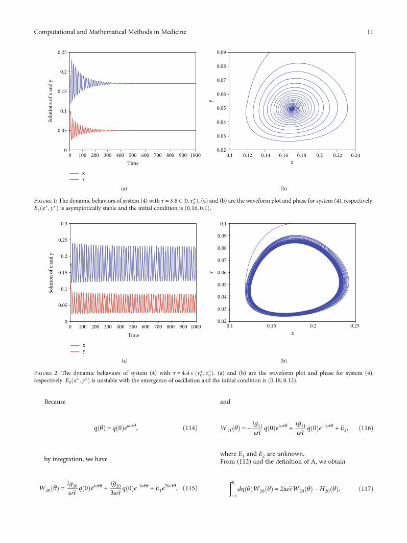
Figure 2: The dynamic behaviors of system (4) with τ = 4:4 ∈ ðτ+0 , τ−0 Þ. (a) and (b) are the waveform plot and phase for system (4),respectively. E3ðx∗, y∗Þ is unstable with the emergence of oscillation and the initial condition is ð0:18, 0:12Þ.

0.25

xy

0.2

0.15

0.1

0.05

Solu

tions

of x

and

y

00 100 200 300 400 500 600

Time700 800 900 1000

(a)

0.09

0.08

0.07

0.06

y

0.05

0.04

0.03

0.020.1 0.12 0.14 0.16 0.18

x0.2 0.22 0.24

(b)

Figure 1: The dynamic behaviors of system (4) with τ = 3:8 ∈ ½0, τ+0 Þ. (a) and (b) are the waveform plot and phase for system (4), respectively.E3ðx∗, y∗Þ is asymptotically stable and the initial condition is ð0:16, 0:1Þ.


and

ð0−1dη θð ÞW11 θð Þ = −H11 θð Þ: ð118Þ

Then, together with (108), we get

H20 0ð Þ = −g20q 0ð Þ − �g02�q 0ð Þ + 2−wN Ne−iω�τ + 1

�−mNÞ

m −wð ÞN −wÞ

!

H11 0ð Þ = −g11q 0ð Þ − �g11�q 0ð Þ + 2−w Re N Ne−iω�τ + 1

�� −m Re Nf gÞ

m −wð ÞRe Nf g −wÞ

!8>>>>><>>>>>:

:

ð119Þ

Substituting (115) and (119) into (117), we have

2iω�τI −ð0−1eiω�τθdη θð Þ

� �E1 = 2

−wN Ne−iω�τ + 1 �

−mNÞm −wð ÞN −wÞ

!: ð120Þ

That is

2iω −m + se−2iω�τ −n + se−2iω�τ

− m −wð Þy∗ 2iω +wy∗

!E1 = 2

−wN Ne−iω�τ + 1 �

−mNÞm −wð ÞN −wÞ

!,

ð121Þ

from which, E1 can be determined.

500

0.6

0.5

0.4

0.3

Solu

tions

of x

and

y

0.2

0.1

0600

Time

700 800 900 1000 1100 1200 1300 1400 1500

xy

(a)

0.25

0.2

0.15

y

0.1

0.05

00.05 0.1 0.15 0.2 0.25 0.3

x0.35 0.4 0.45 0.5

(b)

Figure 4: The dynamic behaviors of system (4) with τ = 23 ∈ ðτ+1 , τ−1 Þ. (a) and (b) are the waveform plot and phase for system (4), respectively.E3ðx∗, y∗Þ is unstable with the emergence of oscillation and the initial condition is ð0:2, 0:2Þ.

0.3

0.25

0.2

0.15

Solu

tion

of x

and

y

0.1

0.05

00 100 200 300 400 500 600

Time700 800 900 1000

xy

(a)

0.09

0.08

0.07

0.06

y

0.05

0.04

0.03

0.020.13 0.14 0.15 0.16 0.17 0.18

x0.19 0.2 0.21 0.22 0.23

(b)

Figure 3: The dynamic behaviors of system (4) with τ = 11 ∈ ðτ−0 , τ+1 Þ. (a) and (b) are the waveform plot and phase for system (4), respectively.E3ðx∗, y∗Þ is asymptotically stable and the initial condition is ð0:1,0:06Þ.


By (115), (117), and (119), we have

ð0−1dη θð Þ

E2 = 2

−w Re N Ne−iω�τ + 1 ��

−mRe Nf gÞm −wð Þ Re Nf g −wÞ

!:

ð122Þ

That is

−m + s −n + s

− m −wð Þy∗ wy∗

!E2 = 2

−w Re N Ne−iω�τ + 1 ��

−m Re Nf gÞm −wð Þ Re Nf g −wÞ

!,

ð123Þ

from which, E2 can be determined.

0.5

0.45

0.4

0.35

0.3

0.25

0.2

0.15

0.1

0.05

0800 900 1000 1100 1200 1300

Time1400 1500 1600 1700 1800

Solu

tions

of x

and

y

xy

(a)

y

0.18

0.16

0.14

0.12

0.1

0.08

0.06

0.04

0.02

00.05 0.1 0.15 0.2 0.25

x0.3 0.35 0.4

(b)

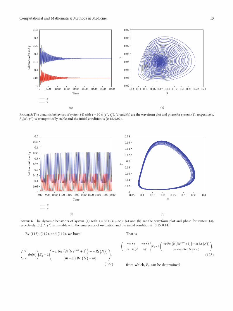
Figure 6: The dynamic behaviors of system (4) with τ = 36 ∈ ðτ+2 ,+∞Þ. (a) and (b) are the waveform plot and phase for system (4),respectively. E3ðx∗, y∗Þ is unstable with the emergence of oscillation and the initial condition is ð0:15, 0:14Þ.

0.35

0.3

0.25

0.2

0.15

0.1

0.05

00 500 1000 1500 2000 2500

Time3000 3500 4000

Solu

tions

of x

and

y

xy

(a)

y

0.09

0.08

0.07

0.06

0.05

0.04

0.03

0.020.13 0.14 0.15 0.16 0.17 0.18 0.19 0.2

x0.21 0.22 0.23

(b)

Figure 5: The dynamic behaviors of system (4) with τ = 30 ∈ ðτ−1 , τ+2 Þ. (a) and (b) are the waveform plot and phase for system (4), respectively.E3ðx∗, y∗Þ is asymptotically stable and the initial condition is ð0:15, 0:02Þ.


Substituting E1 and E2 into (115) and (116), W20 andW11 could be obtained; furthermore, g21 can be calculated.

Then, the important parameters can be obtained:

C1 0ð Þ = i2ω�τ g20g11 − 2 g11j j2 − 1

3 g02j j2 + g212

,

μ2 = −Re C1 0ð Þ½ �Re λ′ �τð Þ

,

β2 = 2 Re C1 0ð Þ½ �,

T2 = −Im C1 0ð Þ + μ2 Im λ′ �τð Þ

h iω�τ

,

ð124Þ

which determine the quantities of the bifurcation of sys-tem (4) at τ = �τ, where μ2 determines the direction of thebifurcation: Hopf bifurcation is subcritical (supercritical) ifμ2 < 0 (μ2 > 0) and the bifurcating periodic solutions existfor τ < �τ (τ > �τ); β2 determines the stability of the bifurcatingperiodic solutions, which are stable (unstable) if β2 < 0(β2 > 0); T2 determines the period of the periodic solutions,which decreases (increases) if T2 < 0 (T2 > 0).

From (78) in Section 4, we know that Re λ′ð�τÞ > 0 whenτ = τ+j , and Re λ′ð�τÞ < 0 when τ = τ−j .

Theorem 8. If ðm −wÞ ffiffiffiffiΔ

p−wB < 0, then the Hopf bifurca-

tion of system (4) at positive equilibrium E3ðx∗, y∗Þ when τ= τ j is supercritical (subcritical) and the bifurcating periodicsolutions on the manifold are stable (unstable) if Re ½C1ð0Þ�< 0 (Re ½C1ð0Þ� > 0).

Theorem 9. If ðm −wÞ ffiffiffiffiΔ

p−wB > 0, Δ1 > 0, and z1 + z2 = 2

p − r2 + s2 > 0, then when τ = τ+j , the Hopf bifurcation of sys-tem (4) at the positive equilibrium E3ðx∗, y∗Þ is supercritical(subcritical) and the bifurcating periodic solutions on the man-ifold are stable (unstable) if Re ½C1ð0Þ� < 0 (Re ½C1ð0Þ� > 0);

when τ = τ−j , the Hopf bifurcation of system (4) at the pos-itive equilibrium E3ðx∗, y∗Þ is subcritical (supercritical) andthe bifurcating periodic solutions on the manifold are stable(unstable) if Re ½C1ð0Þ� < 0 (Re ½C1ð0Þ� > 0).

6. Numerical Simulations

In this section, some numerical simulations are carried out tosupport our theoretical analysis.

There are so many different cases that only the most par-ticular one in (3) of Theorem 7 is considered in this section.The coefficients are chosen as follows: b = 0:4, d = 0:8, w = 1,andm = 6. Then, the conditions of (3) in Theorem 7 are sat-isfied, where

ðm −wÞ ffiffiffiffiΔ

p−wB ≈ 13:166 > 0, Δ1 ≈ 0:0110067

> 0, and2p − r2 + s2 ≈ 0:319612 > 0

.

By direct calculation, we have

x∗ ≈ 0:169906, y∗ ≈ 0:049528 ; ð125Þ

and

τ+0 ≈ 4:25918, τ−0 ≈ 9:66231, τ+1 ≈ 17:8969, τ−1 ≈ 28:8393, τ+2≈ 31:5347, τ−2 ≈ 48:0163, τ+3 ≈ 45:1725⋯,

ð126Þ

where τ−2 > τ+3 .From Theorem 7, we know that the positive equilibrium

E3ð0:169906, 0:049528Þ should be asymptotically stablewhen τ ∈ ½0, τ+0 Þ ∪ ðτ−0 , τ+1 Þ ∪ ðτ−1 , τ+2 Þ, and it is unstable whenτ ∈ ðτ+0 , τ−0 Þ ∪ ðτ+1 , τ−1 Þ ∪ ðτ+2 ,+∞Þ. The system (4) undergoes3 switches.

All the simulation results for τ in the six different inter-vals are in consistent with the theoretical analysis, whichare shown in Figures 1–6.

Data Availability

The data used to support the findings of the study areincluded within the article.

Conflicts of Interest

The authors declare that they have no competing interests.

Authors’ Contributions

All authors conceived the study, carried out the proofs, andapproved the final manuscript.

Acknowledgments

This work is supported by the Fundamental Research Fundsfor the Central Universities under grant no. 3072021CF0609.

References

[1] S. S. Nadim, I. Ghosh, and J. Chattopadhyay, “Short-term pre-dictions and prevention strategies for COVID-19: a model-based study,” Applied Mathematics and Computation, vol. 404,no. 2, p. 126251, 2021.

[2] K. M. Furati, I. O. Sarumi, and A. Q. M. Khaliq, “Fractionalmodel for the spread of COVID-19 subject to governmentintervention and public perception,” Applied MathematicalModelling, vol. 95, pp. 89–105, 2021.

[3] X. Z. Meng, S. Zhao, T. Feng, and T. Zhang, “Dynamics of anovel nonlinear stochastic SIS epidemic model with doubleepidemic hypothesis,” Journal of Mathematical Analysis andApplications, vol. 433, no. 1, pp. 227–242, 2016.

[4] M. Sekiguchi, E. Ishiwata, and Y. Nakata, “Dynamics of an ultra-discrete SIR epidemicmodel with time delay,”Mathematical Bio-sciences and Engineering, vol. 15, no. 3, pp. 653–666, 2018.

[5] Y. L. Cai, Y. Kang, and W. Wang, “A stochastic SIRS epidemicmodel with nonlinear incidence rate,” Applied Mathematics


and Computation, vol. 305, pp. 221–240, 2017.

[6] W. O. Kermack and A. G. McKendrick, “A contribution to themathematical theory of epidemics,” Proceedings of the RoyalSociety of London. Series A, Containing Papers of a Mathemat-ical and Physical Character, vol. 115, no. 772, pp. 700–721,1927.

[7] Y. Enatsu, E. Messina, Y. Muroya, Y. Nakata, E. Russo, andA. Vecchio, “Stability analysis of delayed SIR epidemic modelswith a class of nonlinear incidence rates,” AppliedMathematicsand ComputationApplied Mathematics and Computation,vol. 218, no. 9, pp. 5327–5336, 2012.

[8] W. G. Aiello and H. I. Freedman, “A time-delay model ofsingle-species growth with stage structure,”Mathematical Bio-sciences, vol. 101, no. 2, pp. 139–153, 1990.

[9] H. Zhang, L. Chen, and J. J. Nieto, “A delayed epidemic modelwith stage-structure and pulses for pest management strategy,”Nonlinear Analysis: Real World Applications, vol. 9, no. 4,pp. 1714–1726, 2008.

[10] T. L. Zhang, J. Liu, and Z. Teng, “Stability of Hopf bifurcationof a delayed SIRS epidemic model with stage structure,” Non-linear Analysis: Real World Applications, vol. 11, no. 1,pp. 293–306, 2010.

[11] X. Y. Shi, J. Cui, and X. Zhou, “Stability and Hopf bifurcationanalysis of an eco-epidemic model with a stage structure,”Nonlinear Analysis: Theory, Methods & Applications, vol. 74,no. 4, pp. 1088–1106, 2011.

[12] J. Liu and K. Wang, “Dynamics of an epidemic model withdelays and stage structure,” Computational and Applied Math-ematics, vol. 37, no. 2, pp. 2294–2308, 2018.

[13] B. Cao, H. F. Huo, and H. Xiang, “Global stability of an age-structure epidemic model with imperfect vaccination andrelapse,” Physica A: Statistical Mechanics and its Applications,vol. 486, pp. 638–655, 2017.

[14] A. R. Zhou, P. Sattayatham, and J. Jiao, “Dynamics of an SIRepidemic model with stage structure and pulse vaccination,”Advances in Difference Equations, vol. 2016, no. 1, Article ID140, 2016.

[15] Y. N. Xiao and L. S. Chen, “An SIS epidemic model with stagestructure and a delay,” Acta Mathematicae Applicatae Sinica,English Series, vol. 18, no. 4, pp. 607–618, 2002.

[16] J. W. Jia and Q. Li, “Qualitative analysis of an SIR epidemicmodel with stage structure,”AppliedMathematics and Compu-tation, vol. 193, no. 1, pp. 106–115, 2007.

[17] Z. C. Jiang, W. Ma, and J. Wei, “Global Hopf bifurcation andpermanence of a delayed SEIRS epidemic model,” Mathemat-ics and Computers in Simulation, vol. 122, pp. 35–54, 2016.

[18] Z. Wang, X. Wang, Y. Li, and X. Huang, “Stability and Hopfbifurcation of fractional-order complex-valued single neuronmodel with time delay,” International Journal of Bifurcationand Chaos, vol. 27, no. 13, p. 1750209, 2017.

[19] Z. L. Shen and J. Wei, “Hopf bifurcation analysis in a diffusivepredator-prey system with delay and surplus killing effect,”Mathematical Biosciences and Engineering, vol. 15, no. 3,pp. 693–715, 2018.

[20] Y. Qu and J. Wei, “Bifurcation analysis in a time-delay modelfor prey-predator growth with stage-structure,” NonlinearDynamics, vol. 49, no. 1-2, pp. 285–294, 2007.

[21] B. D. Hassard, N. D. Kazarinoff, and Y. H. Wan, Theory andApplications of Hopf Bifurcation, Cambridge University Press,Cambridge, 1981.


cmmm 1895764 1

Documents