1

Clustering on Multi-Layer Graphs via SubspaceAnalysis on Grassmann ManifoldsXiaowen Dong, Pascal Frossard, Pierre Vandergheynst and Nikolai Nefedov

Abstract—Relationships between entities in datasets are oftenof multiple nature, like geographical distance, social relationships,or common interests among people in a social network, forexample. This information can naturally be modeled by a setof weighted and undirected graphs that form a global multi-layer graph, where the common vertex set represents the entitiesand the edges on different layers capture the similarities of theentities in term of the different modalities. In this paper, weaddress the problem of analyzing multi-layer graphs and proposemethods for clustering the vertices by efficiently merging theinformation provided by the multiple modalities. To this end, wepropose to combine the characteristics of individual graph layersusing tools from subspace analysis on a Grassmann manifold. Theresulting combination can then be viewed as a low dimensionalrepresentation of the original data which preserves the most im-portant information from diverse relationships between entities.We use this information in new clustering methods and test ouralgorithm on several synthetic and real world datasets where wedemonstrate superior or competitive performances compared tobaseline and state-of-the-art techniques. Our generic frameworkfurther extends to numerous analysis and learning problems thatinvolve different types of information on graphs.

Index Terms—Multi-layer graphs, subspace representation,Grassmann manifold, clustering.

I. INTRODUCTION

GRAPHS are powerful mathematical tools for modelingpairwise relationships among sets of entities; they can

be used for various analysis tasks such as classification orclustering. Traditionally, a graph captures a single form ofrelationships between entities and data are analyzed in lightof this one-layer graph. However, numerous emerging appli-cations rely on different forms of information to characterizerelationships between entities. Diverse examples include hu-man interactions in a social network or similarities betweenimages or videos in multimedia applications. The multimodalnature of the relationships can naturally be represented by aset of weighted and undirected graphs that share a commonset of vertices but with different edge weights depending onthe type of information in each graph. This can then be repre-sented by a multi-layer or multi-view graph which gathers allsources of information in a unique representation. Assumingthat all the graph layers are informative, they are likely toprovide complementary information and thus to offer richer

X. Dong, P. Frossard and P. Vandergheynst are with Signal Pro-cessing Laboratories (LTS4/LTS2), Ecole Polytechnique Federale de Lau-sanne (EPFL), Lausanne, Switzerland (e-mail: xiaowen.dong@epfl.ch; pas-cal.frossard@epfl.ch; pierre.vandergheynst@epfl.ch).

N. Nefedov is with Signal and Information Processing Laboratory, Eid-genossische Technische Hochschule Zurich (ETH Zurich), Zurich, Switzerland(e-mail: nefedov@isi.ee.ethz.ch).

(a) (b)

Fig. 1. (a) An illustration for a three-layer graph G, whose three layers{Gi}3i=1 share the same set of vertices but with different edges. (b) Apotential unified clustering {Ck}3k=1 of the vertices based on the informationprovided by the three layers.

information than any single layer taken in isolation. We thusexpect that a proper combination of the information containedin the different layers leads to an improved understanding ofthe structure of the data and the relationships between entitiesin the dataset.

In this paper, we consider a M -layer graph G with individ-ual graph layers Gi = {V,Ei, ωi}, i = 1, . . . ,M , where Vrepresents the common vertex set and Ei represents the edgeset in the i-th individual graph Gi with associated edge weightsωi. An example of a three-layer graph is shown in Fig. 1 (a),where the three graph layers share the same set of 12 verticesbut with different edges (we assume unit edge weights forthe sake of simplicity). Clearly, different graph layers capturedifferent types of relationships between the vertices, and ourobjective is to find a method that properly combines theinformation in these different layers. We first adopt a subspacerepresentation for the information provided by the individualgraph layers, which is inspired by the spectral clusteringalgorithms [1], [2], [3]. We then propose a novel methodfor combining the multiple subspace representations into onerepresentative subspace. Specifically, we model each graphlayer as a subspace on a Grassmann manifold. The problemof combining multiple graph layers is then transformed intothe problem of efficiently merging different subspaces on aGrassmann manifold. To this end, we study the distancesbetween the subspaces and develop a new framework to mergethe subspaces where the overall distance between the repre-sentative subspace and the individual subspaces is minimized.We further show that our framework is well justified by resultsfrom statistical learning theory [4], [5]. The proposed methodis a dimensionality reduction algorithm for the original data;

arX

iv:1

303.

2221

v1 [

cs.L

G]

9 M

ar 2

013

2

it leads to a summarization of the information contained in themultiple graph layers, which reveals the intrinsic relationshipsbetween the vertices in the multi-layer graph.

Various learning problems can then be solved using theserelationships, such as classification or clustering. Specifically,we focus in this paper on the clustering problem: we wantto find a unified clustering of the vertices (as illustrated inFig. 1 (b)) by utilizing the representative subspace, such thatit is better than clustering achieved on any of the graphlayers Gi independently. To address this problem, we firstapply our generic framework of subspace analysis on theGrassmann manifold to compute a meaningful summarization(as a representative subspace) of information contained inthe individual graph layers. We then implement a spectralclustering algorithm based on the representative subspace. Ex-periments on synthetic and real world datasets demonstrate theadvantages of our approach compared to baseline algorithms,like the summation of individual graphs [6], as well as state-of-the-art techniques, such as co-regularization [7]. Finally, webelieve that our framework is beneficial not only to clustering,but also to many other data processing tasks based on multi-layer graphs or multi-view data in general.

This paper is organized as follows. We first review therelated work and summarize the contribution of the paper inSection II. In Section III, we describe the subspace repre-sentation inspired by spectral clustering, which captures thecharacteristics of a single graph. In Section IV, we reviewthe main ingredients of Grassmann manifold theory, andpropose a new framework for combining information frommultiple graph layers. We then propose our novel algorithm forclustering on multi-layer graphs in Section V, and compare itsperformance with other clustering methods on multiple graphsin Section VI. Finally, we conclude in Section VII.

II. RELATED WORK

In this section we review the related work in the literature.First, we describe briefly graph-based clustering algorithms,with a particular focus on the methods that have subspaceinterpretations. Second, we summarize the previous worksbuilt upon subspace analysis and the Grassmann manifoldtheory. Finally, we report the recent progresses in the fieldof analysis of multi-layer graphs or multi-view data.

Clustering on graphs has been studied extensively due to itsnumerous applications in different domains. The works in [8],[9] have given comprehensive overviews of the advancementsin this field over the last few decades. The algorithms thatare based on spectral techniques on graphs are of particularinterest, typical examples being spectral clustering [1], [2], [3]and modularity maximization via spectral method [10], [11].Specifically, these approaches propose to embed the vertices ofthe original graph into a low dimensional space, usually calledthe spectral embedding, which consists of the top eigenvectorsof a special matrix (graph Laplacian matrix for spectral cluster-ing and modularity matrix for modularity maximization). Dueto the special properties of these matrices, clustering in suchlow dimensional spaces usually becomes trivial. Therefore,the corresponding clustering approaches can be interpreted

as transforming the information on the original graph intoa meaningful subspace representation. Another example isthe Principal Component Analysis (PCA) interpretation ongraphs described in [12], which links the graph structure toa subspace spanned by the top eigenvectors of the graphLaplacian matrix. These works have inspired us to considerthe subspace representation in Section III.

In the past few decades, subspace-based methods havebeen widely used in classification and clustering problems,most notably in image processing and computer vision. In[13], [14], the authors have discovered that human faces canbe characterized by low-dimensional subspaces. In [15], theauthors have proposed to use the so-called “eigenfaces” forrecognition. Inspired by these works, researchers have beenparticularly interested in data where data points of the samepattern can be represented by a subspace. Due to the growinginterests in this field, there is an increasingly large numberof works that use tools from the Grassmann manifold theory,which provides a natural tool for subspace analysis. In [16],the authors have given a detailed overview of the basics of theGrassmann manifold theory, and developed new optimizationtechniques on the Grassmann manifold. In [17], the author haspresented statistical analysis on the Grassmann manifold. Bothworks study the distances on the Grassmann manifold. In [18],[4], the authors have proposed learning frameworks based ondistance analysis and positive semidefinite kernels defined onthe Grassmann manifold. Other recent representative worksinclude the studies in [19], [20] where the authors have pro-posed to find optimal subspace representation via optimizationon the Grassmann manifold, and the analysis in [21] wherethe authors have presented statistical methods on the Stiefeland Grassmann manifolds for applications in vision. Similarly,the work in [22] has proposed a novel discriminant analysisframework based on graph embedding for set matching, andthe authors in [23] have presented a subspace indexing modelon the Grassmann manifold for classification. However, noneof the above works considers datasets represented by multi-layer graphs.

At the same time, multi-view data have attracted a largeamount of interest in the learning research communities.These data form multi-layer graph representations (or multi-view representations), which generally refer to data that canbe analyzed from different viewpoints. In this setting, thekey challenge is to combine efficiently the information frommultiple graphs (or multiple views) for learning purposes. Theexisting techniques can be roughly grouped into the followingcategories. First, the most straightforward way is to form aconvex combination of the information from the individualgraphs. For example, in [24], the authors have developed amethod to learn an optimal convex combination of Laplaciankernels from different graphs. In [25], the authors have pro-posed a Markov mixture model, which corresponds to a convexcombination of the normalized adjacency matrices of theindividual graphs, for supervised and unsupervised learning. In[26], the authors have presented several averaging techniquesfor combining information from the individual graphs forclustering. Second, following the intuitive approaches in thefirst category, many existing works aim at finding a unified

3

representation of the multiple graphs (or multiple views), butusing more sophisticated methods. For instances, the authorsin [6], [27], [28], [29], [30], [31] have developed severaljoint matrix factorization approaches to combine differentviews of data through a unified optimization framework, wherethe authors in [32] have proposed to find a unified spectralembedding of the original data by integrating informationfrom different views. Similarly, clustering algorithms basedon Canonical Correlation Analysis (CCA) first project the datafrom different views into a unified low dimensional subspace,and then apply simple algorithms like single linkage or k-means to achieve the final clustering [33], [34]. Third, unlikethe previous methods that try to find a unified representa-tion before applying learning techniques, another strategy inthe literature is to integrate the information from individualgraphs (views) directly into the optimization problems forthe learning purposes. Examples include the co-EM clusteringalgorithm proposed in [35], and the clustering approachesproposed in [36], [7] based on the frameworks of co-training[37] and co-regularization [38]. Fourth, particularly in theanalysis of multiple graphs, regularization frameworks ongraphs have also been applied. In [39], the authors havepresented a regularization framework over edge weights ofmultiple graphs to compute an improved similarity graphof the vertices (entities). In [29], [40], the authors haveproposed graph regularization frameworks in both vertex andgraph spectral domain to combine individual graph layers.Finally, other representative approaches include the works in[41], [39] where the authors have defined additional graphrepresentations to incorporate information from the originalindividual graphs, and the works in [42], [43], [44], [45] wherethe authors have proposed ensemble clustering approachesby integrating clustering results from individual views. Fromthis perspective, the proposed approach belongs to the secondcategory mentioned above, where we first find a representativesubspace for the information provided by the multi-layer graphand then implement the clustering step, or other learning tasks.We believe that this type of approaches is intuitive and easilyunderstandable, yet still flexible and generic enough to beapplied to different types of data.

To summarize, the main differences between the relatedwork and the contributions proposed in this paper are the fol-lowing. First, the research work on Grassmann manifold theoryhas been mainly focused on subspace analysis. The subspaceusually comes directly from the data but are not linked tograph-based learning problems. Our paper makes the explicitlink between subspaces and graphs, and presents a fundamen-tal and intuitive way of approaching the learning problemson multi-layer graphs, with help of subspace analysis on theGrassmann manifold. Second, we show the link between theprojection distance on the Grassmann manifold [16], [18] andthe empirical estimate of the Hilbert-Schmidt IndependenceCriterion (HSIC) [5]. Therefore, together with the results in[4], we are able to offer a unified view of concepts from threedifferent perspectives, namely, the projection distance on theGrassmann manifold, the Kullback-Leibler (K-L) divergence[46] and the HSIC [5]. This helps to understand better thekey concept of distance measure in subspace analysis. Finally,

using our novel layer merging framework, we provide a simpleyet competitive solution to the problem of clustering on multi-layer graphs. We also discuss the influence of the relationshipsbetween the individual graph layers on the performance ofthe proposed clustering algorithm. We believe that this ishelpful towards the design of efficient and adaptive learningalgorithms.

III. SUBSPACE REPRESENTATION FOR GRAPHS

In this section, we describe a subspace representation forthe information provided by a single graph. The subspacerepresentation is inspired by spectral clustering, which studiesthe spectral properties of the graph information for partitioningthe vertex set of the graph into several distinct subsets.

Let us consider an weighted and undirected graph G =(V,E, ω)1, where V = {vi}ni=1 represents the vertex set andE represents the edge set with associated edge weights ω,respectively. Without loss of generality, we assume that thegraph is connected. The adjacency matrix W of the graphis a symmetric matrix whose entry Wij represents the edgeweight if there is an edge between vertex vi and vj , or 0otherwise. The degree of a vertex is defined as the sum of theweights of all the edges incident to it in the graph, and thedegree matrix D is defined as the diagonal matrix containingthe degrees of each vertex along its diagonal. The normalizedgraph Laplacian matrix L is then defined as:

L = D−12 (D −W )D−

12 . (1)

The graph Laplacian is of broad interests in the studies ofspectral graph theory [47]. Among several variants, we usethe normalized graph Laplacian defined in Eq. (1), since itsspectrum (i.e., its eigenvalues) always lie between 0 and 2, aproperty favorable in comparing different graph layers in thefollowing sections. We consider now the problem of clusteringthe vertices V = {vi}ni=1 of G into k distinct subsets suchthat the vertices in the same subset are similar, i.e., theyare connected by edges of large weights. This problem canbe efficiently solved by the spectral clustering algorithms.Specifically, we focus on the algorithm proposed in [2], whichsolves the following trace minimization problem:

minU∈Rn×k

tr(U ′LU), s.t. U ′U = I, (2)

where n is the number of vertices in the graph, k is thetarget number of clusters, and (·)′ denotes the matrix transposeoperator. It can be shown by a version of the Rayleigh-Ritztheorem [3] that the solution U to the problem of Eq. (2)contains the first k eigenvectors (which correspond to thek smallest eigenvalues) of L as columns. The clustering ofthe vertices in G is then achieved by applying the k-meansalgorithm [48] to the normalized row vectors of the matrixU 2. As shown in [3], the behavior of spectral clusteringcan be explained theoretically with analogies to several well-known mathematical problems, such as the normalized graph-cut problem [1], the random walk process on graphs [49], and

1We use the notation G for a single graph exclusively in this section.

4

problems in perturbation theory [50], [51]. This algorithm issummarized in Algorithm 1.

Algorithm 1 Normalized Spectral Clustering [2]1: Input:W : the n× n weighted adjacency matrix of graph Gk: target number of clusters

2: Compute the degree matrix D and the normalized graphLaplacian matrix L = D−

12 (D −W )D−

12 .

3: Let U ∈ Rn×k be the matrix containing the first keigenvectors u1, . . . , uk of L (solution of (2)). Normalizeeach row of U to get Unorm.

4: Let yj ∈ Rk (j = 1, . . . , n) be the j-th row of Unorm.5: Cluster yj in Rk into k clusters C1, . . . , Ck using the k-

means algorithm.6: Output:C1, . . . , Ck: the cluster assignment

We provide an illustrative example of the spectral clusteringalgorithm. Consider a single graph in Fig. 2 (a) with tenvertices that belong to three distinct clusters (i.e., n=10 andk=3). For the sake of simplicity, all the edge weights are setto 1. The low dimensional matrix U that solves the problemof Eq. (2), which contains k orthonormal eigenvectors of thegraph Laplacian L as columns, is shown in Fig. 2 (b). Thematrix U is usually called the spectral embedding of thevertices, as each row of U can be viewed as the set of coordi-nates of the corresponding vertex in the k-dimensional space.More importantly, due to the properties of the graph Laplacianmatrix, such an embedding preserves the connectivity of thevertices in the original graph. In other words, two vertices thatare strongly connected in the graph are mapped to two vectors(i.e., rows of U ) that are close too in the k-dimensional space.As a result, a simple k-means algorithm can be applied to thenormalized row vectors of U to achieve the final clustering ofthe vertices.

Inspired by the spectral clustering theory, one can definea meaningful subspace representation of the original verticesin a graph by its k-dimensional spectral embedding, which isdriven by the matrix U built on the first k eigenvectors ofthe graph Laplacian L. Each row being the coordinates of thecorresponding vertex in the low dimensional subspace, thisrepresentation contains the information on the connectivityof the vertices in the original graph. Such information canbe used for finding clusters of the vertices, as shown above,but it is also useful for other analysis tasks on graphs. Byadopting this subspace representation that “summarizes” thegraph information, multiple graph layers can naturally berepresented by multiple such subspaces (whose geometricalrelationships can be quite flexible). The task of multi-layergraph analysis can then be transformed into the problem ofeffective combination of the multiple subspaces. This is thefocus of the next section.

2The necessity for row normalization is discussed in [3] and we omit thisdiscussion here. However, the normalization does not change the nature ofspectral embedding, hence, it does not affect our derivation later.

(a) (b)

Fig. 2. An illustration of spectral clustering. (a) A graph with three clusters(color-coded) of vertices; (b) Spectral embedding of the vertices computedfrom the graph Laplacian matrix. The vertices in the same cluster are mappedto coordinates that are close to each other in R3.

IV. MERGING SUBSPACES VIA ANALYSIS ON THEGRASSMANN MANIFOLD

We have described above the subspace representation foreach graph layer in the multi-layer graph. We discuss nowthe problem of effectively combining multiple graph layersby merging multiple subspaces. The theory of Grassmannmanifold provides a natural framework for such a problem.In this section, we first review the main ingredients of theGrassmann manifold theory, and then move onto our genericframework for merging subspaces.

A. Ingredients of Grassmann manifold theory

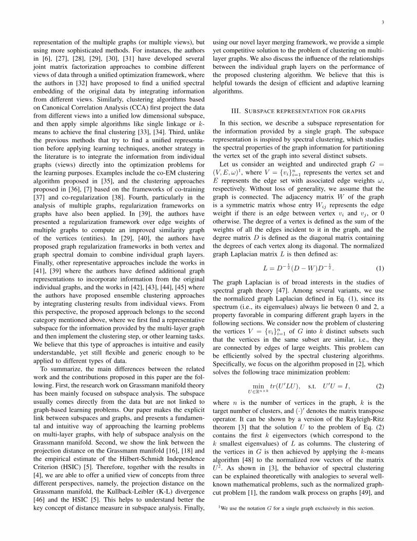
By definition, a Grassmann manifold G(k, n) is the set ofk-dimensional linear subspaces in Rn, where each uniquesubspace is mapped to a unique point on the manifold. Asan example, Fig. 3 shows two 2-dimensional subspaces inR3 being mapped to two points on G(2, 3). The advantageof using tools from Grassmann manifold theory is thus two-fold: (i) it provides a natural representation for our problem:the subspaces representing the individual graph layers can beconsidered as different points3 on the Grassmann manifold;(ii) the analysis on the Grassmann manifold permits to useefficient tools to study the distances between points on themanifold, namely, distances between different subspaces. Suchdistances play an important role in the problem of mergingthe information from multiple graph layers. In what follows,we focus on the definition of one particular distance measurebetween subspaces, which will be used in our framework lateron.

Mathematically speaking, each point on G(k, n) can berepresented by an orthonormal matrix Y ∈ Rn×k whosecolumns span the corresponding k-dimensional subspace inRn; it is thus denoted as span(Y ). For example, the twosubspaces shown in Fig. 3 can be denoted as span(Y1)and span(Y2) for two orthonormal matrices Y1 and Y2. Thedistance between two points on the manifold, or between twosubspaces span(Y1) and span(Y2), is then defined based on aset of principal angles {θi}ki=1 between these subspaces [52].These principal angles, which measure how the subspaces aregeometrically close, are the fundamental measures used todefine various distances on the Grassmann manifold, such as

3We assume that the Laplacian matrices of any pair of the two layers inthe multi-layer graph have different sets of top eigenvectors. In this case,subspace representations for all the layers will be different from each other.

5

Fig. 3. An example of two 2-dimensional subspaces span(Y1) andspan(Y2) in R3, which are mapped to two points on the Grassmann manifoldG(2, 3).

the Riemannian (geodesic) distance or the projection distance[16], [18]. In this paper, we use the projection distance, whichis defined as:

dproj(Y1, Y2) = (

k∑i=1

sin2θi)12 , (3)

where Y1 and Y2 are the orthonormal matrices represent-ing the two subspaces under comparison4. The reason forchoosing the projection distance is two-fold: (i) the projectiondistance is defined as the `2-norm of the vector of sines ofthe principal angles. Since it uses all the principal angles,it is therefore an unbiased definition. This is favorable aswe do not assume any prior knowledge on the distributionof the data, and all the principal angles are considered tocarry meaningful information; (ii) the projection distance canbe interpreted using a one-to-one mapping that preservesdistinctness: span(Y )→ Y Y ′ ∈ Rn×n. Note that the squaredprojection distance can be rewritten as:

d2proj(Y1, Y2) =

k∑i=1

sin2θi

= k −k∑

i=1

cos2θi

= k − tr(Y1Y1′Y2Y2′)

=1

2[2k − 2tr(Y1Y1

′Y2Y2′)]

=1

2[tr(Y1

′Y1) + tr(Y2′Y2)− 2tr(Y1Y1

′Y2Y2′)]

=1

2||Y1Y1′ − Y2Y2′||2F , (4)

where the third equality comes from the definition of theprincipal angles and the fifth equality uses the fact thatY1 and Y2 are orthonormal matrices. It can be seen fromEq. (4) that the projection distance can be related to theFrobenius norm of the difference between the mappings ofthe two subspaces span(Y1) and span(Y2) in Rn×n. Becausethe mapping preserves distinctness, it is natural to take theprojection distance as a proper distance measure betweensubspaces. Moreover, the third equality of Eq. (4) provides anexplicit way of computing the projection distance between twosubspaces from their matrix representations Y1 and Y2. We are

4In the special case where Y1 and Y2 represent the same subspace, we havedproj(Y1, Y2) = 0.

going to use it in developing the generic merging frameworkin the following section.

To summarize, the Grassmann manifold provides a naturaland intuitive representation for subspace-based analysis (asshown in Fig. 3). The associated tools, namely the principalangles, permit to define a meaningful distance measure thatcaptures the geometric relationships between the subspaces.Originally defined as a distance measure between two sub-spaces, the projection distance can be naturally generalized tothe analysis of multiple subspaces, as we show in the nextsection.

B. Generic merging framework

Equipped with the subspace representation for individualgraphs and with a distance measure to compare differentsubspaces, we are now ready to present our generic frameworkfor merging the information from multiple graph layers. Givena multi-layer graph G with M individual layers {Gi}Mi=1,we first compute the graph Laplacian matrix Li for eachGi and then represent each Gi by the spectral embeddingmatrix Ui ∈ Rn×k from the first k eigenvectors of Li, wheren is the number of vertices and k is the target number ofclusters. Recall that each of the matrices {Ui}Mi=1 definesa k-dimensional subspace in Rn, which can be denoted asspan(Ui). The goal is to merge these multiple subspaces ina meaningful and efficient way. To this end, our philosophyis to find a representative subspace span(U) that is close toall the individual subspaces span(Ui), and at the same timethe representation U preserves the vertex connectivity in eachgraph layer. For notational convenience, in the rest of thepaper we simply refer to the representations U and Ui as thecorresponding subspaces, unless indicated specifically.

The squared projection distance between subspaces definedin Eq. (4) can be naturally generalized for analysis of mul-tiple subspaces. More specifically, we can define the squaredprojection distance between the target representative subspaceU and the M individual subspaces {Ui}Mi=1 as the sum ofsquared projection distances between U and each individualsubspace given by Ui:

d2proj(U, {Ui}Mi=1) =

M∑i=1

d2p(U,Ui)

=

M∑i=1

[k − tr(UU ′UiUi′)]

= kM −M∑i=1

tr(UU ′UiUi′). (5)

The minimization of the distance measure in Eq. (5) enforcesthe representative subspace U to be close to all the individualsubspaces {Ui}Mi=1 in terms of the projection distance onthe Grassmann manifold. At the same time, we want U topreserve the vertex connectivity in each graph layer. Thiscan be achieved by minimizing the Laplacian quadratic formevaluated on the columns of U , as also indicated by theobjective function in Eq. (2) for spectral clustering. Therefore,we finally propose to merge multiple subspaces by solving the

6

following optimization problem that integrates Eq. (2) and Eq.(5):

minU∈Rn×k

M∑i=1

tr(U ′LiU) + α[kM −M∑i=1

tr(UU ′UiUi′)],

s.t. U ′U = I,

(6)

where Li and Ui are the graph Laplacian and the subspacerepresentation for Gi, respectively. The regularization param-eter α balances the trade-off between the two terms in theobjective function.

The problem of Eq. (6) can be solved in a similar man-ner as Eq. (2). Specifically, by ignoring constant terms andrearranging the trace form in the second term of the objectivefunction, Eq. (6) can be rewritten as

minU∈Rn×k

tr[U ′(

M∑i=1

Li − αM∑i=1

UiUi′)U ], s.t. U ′U = I.

(7)It is interesting to note that this is the same trace minimizationproblem as in Eq. (2), but with a “modified” Laplacian:

Lmod =

M∑i=1

Li − αM∑i=1

UiUi′. (8)

Therefore, by the Rayleigh-Ritz theorem, the solution to theproblem of Eq. (7) is given by the first k eigenvectors ofthe modified Laplacian Lmod, which can be computed usingefficient algorithms for eigenvalue problems [53], [54].

In the problem of Eq. (6) we try to find a representativesubspace U from the multiple subspaces {Ui}Mi=1. Such arepresentation not only preserves the structural informationcontained in the individual graph layers, which is encouragedby the first term of the objective function in Eq. (6), but alsokeeps a minimum distance between itself and the multiplesubspaces, which is enforced by the second term. Notice thatthe minimization of only the first term itself corresponds tosimple averaging of the information from different graph lay-ers, which usually leads to suboptimal clustering performanceas we shall see in the experimental section. Similarly, imposingonly a small projection distance to the individual subspaces{Ui}Mi=1 does not necessarily guarantee that U is a goodsolution for merging the subspaces. In fact, for a given k-dimensional subspace, there are infinitely many choices for thematrix representation, and not all of them are considered asmeaningful summarizations of the information provided by themultiple graph layers. However, under the additional constraintof minimizing the trace of the quadratic term U ′LiU over allthe graphs (which is the first term of the objective function inEq. (6)), the vertex connectivity in the individual graphs tendsto be preserved in U . In this case, the smaller the projectiondistance between U and the individual subspaces, the morerepresentative it is for all graph layers.

C. Discussion of the distance function

Interestingly, the choice of projection distance as a similaritymeasure between subspaces in the optimization problem ofEq. (6) can be well justified from information-theoretic and

statistical learning points of view. The first justification isfrom the work of Hamm et al. [4], in which the authors haveshown that the Kullback-Leibler (K-L) divergence [46], whichis a well-known similarity measure between two probabilitydistributions in information theory, is closely related to thesquared projection distance. More specifically, the work in[4] suggests that, under certain conditions, we can consider alinear subspace Ui as the “flattened” limit of a Factor Analyzerdistribution pi [55]:

pi : N (ui, Ci), Ci = UiUi′ + σ2ID, (9)

where N stands for the normal distribution, ui ∈ Rn is themean, Ui ∈ Rn×k is a full-rank matrix with n > k > 0 (whichrepresents the subspace), σ is the ambient noise level, and Inis the identity matrix of dimension n. For two subspaces Ui

and Uj , the symmetrized K-L divergence between the twocorresponding distributions pi and pj can then be rewrittenas:

dKL(p1, p2) =1

2σ2(σ2 + 1)(2k − 2tr(UiUi

′UjUj′)), (10)

which is of the same form as the squared projection distancewhen we ignore the constant factor (see Eq. (4)). This showsthat, if we take a probabilistic view of the subspace representa-tions {Ui}Mi=1, then the projection distance between subspacescan be considered consistent with the K-L divergence.

The second justification is from the recently proposedHilbert-Schmidt Independence Criterion (HSIC) [5], whichmeasures the statistical dependence between two random vari-ables. Given KX1

,KX2∈ Rn×n that are the centered Gram

matrices of some kernel functions defined over two randomvariables X1 and X2, the empirical estimate of HSIC is givenby

dHSIC(X1,X2) = tr(KX1KX2). (11)

That is, the larger the dHSIC(X1,X2), the stronger the statisticaldependence between X1 and X2. In our case, using theidea of spectral embedding, we can consider the rows ofthe individual subspace representations Ui and Uj as twoparticular sets of sample points in Rk, which are drawn fromtwo probability distributions governed by the information onvertex connectivity in Gi and Gj , respectively. In other words,the sets of rows of Ui and Uj can be seen as realizations oftwo random variables Xi and Xj . Therefore, we can define theGram matrices of linear kernels on Xi and Xj as:

KXi= (Ui

′)′(Ui′) = UiUi

′,

KXj= (Uj

′)′(Uj′) = UjUj

′. (12)

By applying Eq. (11), we can see that:

dHSIC(Xi,Xj) = tr(KXiKXj

)

= tr(UiUi′UjUj

′)

= k − d2proj(Ui, Uj). (13)

This shows that the projection distance between subspaces Ui

and Uj can be interpreted as the negative dependence betweenXi and Xj , which reflect the information provided by the twoindividual graph layers Gi and Gj .

7

Therefore, from both information-theoretic and statisticallearning points of view, the smaller the projection distancebetween two subspace representations Ui and Uj , the moresimilar the information in the respective graphs that theyrepresent. As a result, the representative subspace (the solutionU to the problem of Eq. (6)) can be considered as a subspacerepresentation that “summarizes” the information from theindividual graph layers, and at the same time captures theintrinsic relationships between the vertices in the graph. Asone can imagine, such relationships are of crucial importancein our multi-layer graph analysis.

In summary, the concept of treating individual graphs assubspaces, or points on the Grassmann manifold, permitsto study the desired merging framework in a unique andprincipled way. We are able to find a representative subspacefor the multi-layer graph of interest, which can be viewed asa dimensionality reduction approach for the original data. Wefinally remark that the proposed merging framework can beeasily extended to take into account the relative importanceof each individual graph layer with respect to the specificlearning purpose. For instance, when prior knowledge aboutthe importance of the information in the individual graphsis available, we can adapt the value of the regularizationparameter α in Eq. (6) to the different layers such thatthe representative subspace is closer to the most informativesubspace representations.

V. CLUSTERING ON MULTI-LAYER GRAPHS

In Section IV, we introduced a novel framework for mergingsubspace representations from the individual layers of a multi-layer graph, which leads to a representative subspace thatcaptures the intrinsic relationships between the vertices of thegraph. This representative subspace provides a low dimen-sional form that can be used in several applications involvingmulti-layer graph analysis. In particular, we study now onesuch application, namely the problem of clustering vertices ina multi-layer graph. We further analyze the behavior of theproposed clustering algorithm with respect to the propertiesof the individual graph layers (subspaces).

A. Clustering algorithm

As we have already seen in Section III, the success of thespectral clustering algorithm relies on the transformation ofthe information contained in the graph structure into a spectralembedding computed from the graph Laplacian matrix, whereeach row of the embedding matrix (after normalization) istreated as the coordinates of the corresponding vertex in alow dimensional subspace. In our problem of clustering ona multi-layer graph, the setting is slightly different, since weaim at finding a unified clustering of the vertices that takesinto account information contained in all the individual layersof the multi-layer graph. However, the merging frameworkproposed in the previous section can naturally be appliedin this context. In fact, it leads to a natural solution to theclustering problem on multi-layer graphs. In more details,similarly to the spectral embedding matrix in the spectralcluttering algorithm, which is a subspace representation for

one individual graph, our merging framework provides arepresentative subspace that contains the information from themultiple graph layers. Using this representation, we can thenfollow the same steps of spectral clustering to achieve thefinal clustering of the vertices with a k-means algorithm. Theproposed clustering algorithm is summarized in Algorithm 2.

Algorithm 2 Spectral Clustering on Multi-Layer graphs (SC-ML)

1: Input:{Wi}Mi=1: n×n weighted adjacency matrices of individualgraph layers {Gi}Mi=1

k: target number of clustersα: regularization parameter

2: Compute the normalized Laplacian matrix Li and thesubspace representation Ui for each Gi.

3: Compute the modified Laplacian matrix Lmod =∑Mi=1 Li − α

∑Mi=1 UiUi

′.4: Compute U ∈ Rn×k that is the matrix containing the firstk eigenvectors u1, . . . , uk of Lmod. Normalize each rowof U to get Unorm.

5: Let yj ∈ Rk (j = 1, . . . , n) be the j-th row of Unorm.6: Cluster yj in Rk into C1, . . . , Ck using the k-means

algorithm.7: Output:C1, . . . , Ck: The cluster assignment

It is clear that Algorithm 2 is a direct generalization ofAlgorithm 1 in the case of multi-layer graphs. The main in-gredient of our clustering algorithm is the merging frameworkproposed in Section IV, in which information from individualgraph layers is summarized, prior to the actual clusteringprocess (i.e., the k-means step) is implemented. This providesan example that illustrates how our generic merging frameworkcan be applied to specific learning tasks on multi-layer graphs.

B. Analysis of the proposed algorithm

We now analyze the behavior of the proposed clusteringalgorithm under different conditions. Specifically, we firstoutline the link between subspace distance and clusteringquality, and then compare the clustering performances intwo scenarios where the relationships between the individualsubspaces {Ui}Mi=1 are different.

As we have seen in Section IV, the rows of the subspacerepresentations {Ui}Mi=1 can be viewed as realizations ofrandom variables {Xi}Mi=1 governed by the graph information.At the same time, spectral clustering directly utilizes Ui for thepurpose of clustering. Therefore, {Xi}Mi=1 can be consideredas random variables that control the cluster assignment of thevertices. In fact, it has been shown in [3] that the matrix Ui isclosely related to the matrix that contains the cluster indicatorvectors as columns. Since the projection distance can beunderstood as the negative statistical dependence between suchrandom variables, the minimization of the projection distancein Eq. (6) is equivalent to the maximization of the dependencebetween the random variable from the representative subspaceU and the ones from the individual subspaces {Ui}Mi=1. The

8

Fig. 4. A 3-layer graph with unit edge weights for toy example 1. The colorsindicate the groundtruth clusters.

TABLE IANALYSIS OF TOY EXAMPLE 1.

(a) clustering performances for toy example 1

(b) subspace distances for toy example 1

optimization in Eq. (6) can then be seen as a solution that tendsto produce a clustering with the representative subspace that isconsistent with those computed from the individual subspacerepresentations.

We now discuss how the relationships between the individ-ual subspaces possibly affect the performance of our clusteringalgorithm SC-ML. Intuitively, since the second term of theobjective function in Eq. (6) represents the distance betweenthe representative subspace U and all the individual subspaces{Ui}Mi=1, it tends to drive the solution towards those subspacesthat themselves are close to each other on the Grassmannmanifold. To show it more clearly, let us consider two toyexamples. The first example is illustrated in Fig. 4, where wehave a 3-layer graph with the individual layers G1, G2 and G3

sharing the same set of vertices. For the sake of simplicity, allthe edge weights are set to one. In addition, three groundtruthclusters are indicated by the colors of the vertices. Table I (a)shows the performances of Algorithm 1 with individual layersas well as Algorithm 25 for the multi-layer graph, in termsof Normalized Mutual Information (NMI) [56] with respectto the groundtruth clusters. Table I (b) shows the projectiondistances between various pairs of subspaces. It is clear thatthe layers G1 and G2 produce better clustering quality, and thatthe distance between the corresponding subspaces is smaller.However, the vertex connectivity in layer G3 is not veryconsistent with the groundtruth clusters and the correspondingsubspace is further away from the ones from G1 and G2. Inthis case, the solution found by SC-ML is enforced to beclose to the consistent subspaces from G1 and G2, henceprovides satisfactory clustering results (NMI = 1 representsperfect recovery of groundtruth clusters). Let us now considera second toy example, as illustrated in Fig. 5. In this examplewe have two layers G2 and G3 with relatively low qualityinformation with respect to the groundtruth clustering ofthe vertices. As we see in Table II (b), their corresponding

Fig. 5. A 3-layer graph with unit edge weights for toy example 2. The colorsindicate the groundtruth clusters.

TABLE IIANALYSIS OF TOY EXAMPLE 2.

(a) clustering performances for toy example 2

(b) subspace distances for toy example 2

subspaces are close to each other on the Grassmann manifold.The most informative layer G1, however, represents a subspacethat is quite far away from the ones from G2 and G3. At thesame time, we see in Table II (a) that the clustering results arebetter for the first layer than for the other two less informativelayers. If the quality of the information in the different layersis not considered in computing the representative subspace,SC-ML enforces the solution to be closer to two layersof relatively lower quality, which results in unsatisfactoryclustering performance in this case.

The analysis above implies that the proposed clusteringalgorithm works well under the following assumptions: (i) themajority of the individual subspaces are relatively informa-tive, namely, they are helpful for recovering the groundtruthclustering, and (ii) they are reasonably close to each other onthe Grassmann manifold, namely, they provide complementarybut not contradictory information. These are the assumptionsmade in the present work. As we shall see in the next section,these assumptions seem to be appropriate and realistic in realworld datasets. If it is not the case, one may assume thata preprocessing step cleans the datasets, or at least providesinformation about the reliability of the information in thedifferent graph layers.

VI. EXPERIMENTAL RESULTS

In this section, we evaluate the performance of the SC-ML algorithm presented in Section V on several syntheticand real world datasets. We first describe the datasets that weuse for the evaluation, and then explain the various clusteringalgorithms that we adopt in the performance comparisons. Wefinally present the results in terms of three evaluation criteriaas well as some discussions.

5We choose the value of the regularization parameter that leads to the bestpossible clustering performance. More discussions about the choices of thisparameter are presented in Section VI.

9

A. Datasets

We adopt one synthetic and two real world datasets withmulti-layer graph representation for the evaluation of theclustering algorithms. We give a brief overview of the datasetsas follows.

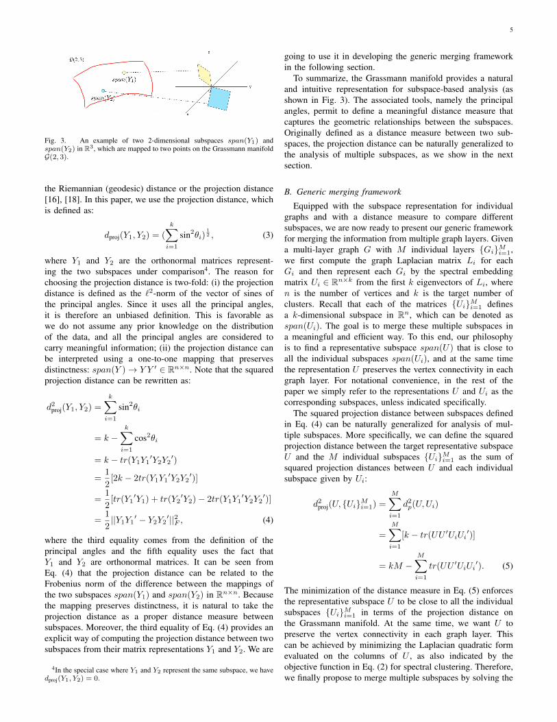
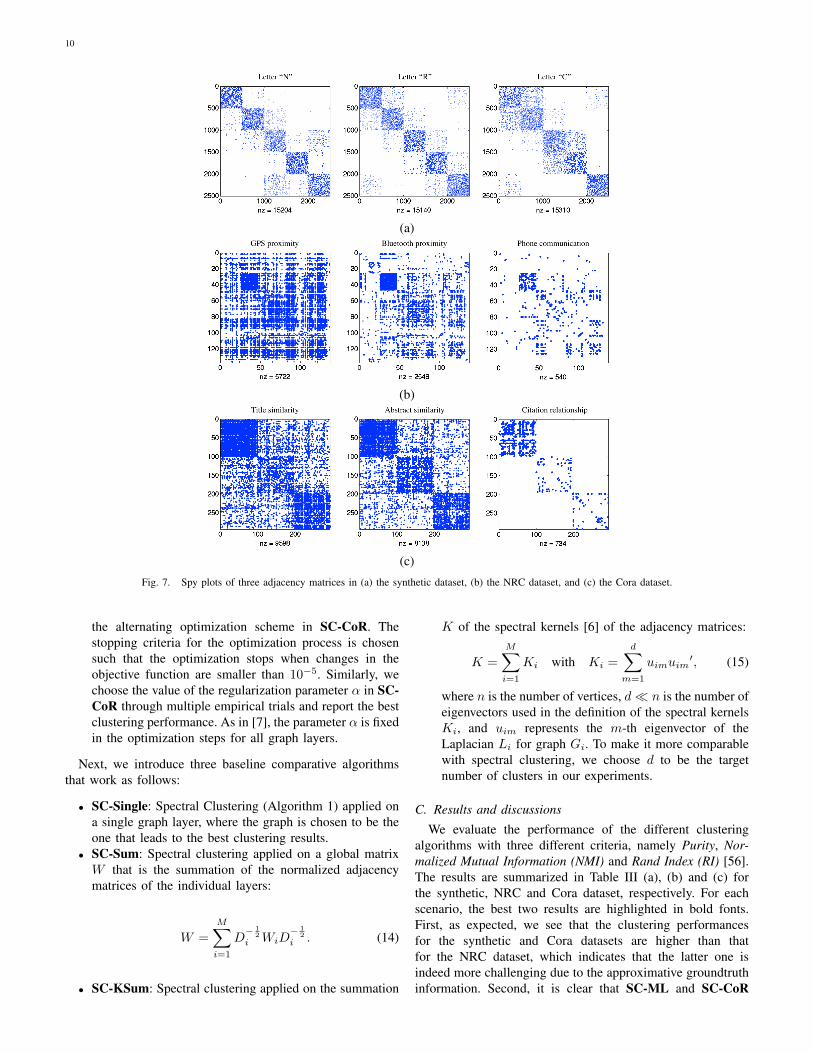
The first dataset that we use is a synthetic dataset, wherewe have three point clouds in R2 forming the English letters“N”, “R” and “C” (shown in Fig. 6). Each point cloud isgenerated from a five-component Gaussian mixture model withdifferent values for the mean and variance of the Gaussiandistributions, where each component represents a class of 500points with specific color. A 5-nearest neighbor graph is thenconstructed for each point cloud by assigning the weight ofthe edges connecting two vertices (points) as the reciprocal ofthe Euclidean distance between them. This gives us a 3-layergraph of 2500 vertices, where each graph layer is from a pointcloud forming a particular letter. The goal with this dataset isto recover the five clusters (indicated by five colors) of the2500 vertices using the three graph layers constructed fromthe three point clouds.

The second dataset contains data collected during the Lau-sanne Data Collection Campaign [57] by the Nokia ResearchCenter (NRC) in Lausanne. This dataset contains the mobilephone data of 136 users living and working in the LakeLeman region in Switzerland, recorded over a one-year period.Considering the users as vertices in the graph, we constructthree graphs by measuring the proximities between these usersin terms of GPS locations, Bluetooth scanning activities andphone communication. More specifically, for GPS locationsand bluetooth scans, we measure how many times two usersare sufficiently close geographically (within a distance ofroughly 1 km), and how many times two users’ devices havedetected the same bluetooth devices, respectively, within 30-minute time windows. Aggregating these results for a one-year period leads to two weighted adjacency matrices thatrepresent the physical proximities of the users measured withdifferent modalities. In addition, an adjacency matrix forphone communication is generated by assigning edge weightsdepending on the number of calls between any pair of twousers. These three adjacency matrices form a 3-layer graph of136 vertices, where the goal is to recover the eight groundtruthclusters that have been constructed from the users’ emailaffiliations.

The third dataset is a subset of the Cora bibliographicdataset6. This dataset contains 292 research papers fromthree different fields, namely, natural language processing,data mining and robotics. Considering papers as vertices inthe graph, we construct the first two graphs by measuringthe similarities among the title and the abstract of thesepapers. More clearly, for both title and abstract, we representeach paper by a vector of non-trivial words using the TermFrequency-Inverse Document Frequency (TF-IDF) weightingscheme, and compute the cosine similarities between everypair of vectors as the edge weights in the graphs. Moreover,we add a third graph which reflects the citation relationshipsamong the papers, namely, we assign an edge with unit weightbetween papers A and B if A has cited or been cited by B.

Fig. 6. Three five-class point clouds in R2 forming English letters “N”, “R”and “C”.

This results in a 3-layer graph of 292 vertices, and the goalin this dataset is to recover the three clusters corresponding tothe different fields the papers belong to.

To visualize the graphs in the three datasets, the spy plotof the adjacency matrices of the graphs are shown in Fig. 7(a), (b) and (c) for the synthetic, NRC and Cora dataset,respectively, where the orderings of the vertices are madeconsistent with the groundtruth clusters7. A spy plot is a globalview of a matrix where every non-zero entry in the matrixis represented by a blue dot (without taking into accountthe value of the entry). As shown in these figures, we seeclearly the clusters in the synthetic and Cora datasets, whilethe clusters in the NRC dataset are not very clear. The reasonfor this is that, in the NRC dataset, the email affiliations usedto create the groundtruth clusters only provides approximativeinformation.

B. Clustering algorithms

We now explain briefly the clustering algorithms in ourcomparative performance analysis along with some imple-mentation details. We adopt three baseline algorithms as wellas a state-of-the-art technique, namely the co-regularizationapproach introduced in [7]. As we shall see, there is an inter-esting connection between this approach and the proposed al-gorithm. First of all, we describe some implementation detailsof the proposed SC-ML algorithm and the co-regularizationapproach in [7]:• SC-ML: Spectral Clustering on Multi-Layer graphs, as

presented in Section V. The implementation of SC-ML is pretty straightforward, and the only parameterto choose is the regularization parameter α in Eq. (6).In our experiments, we choose the value of α throughmultiple empirical trials and report the best clusteringperformance. Specifically, we choose α to be 0.64 forthe synthetic dataset and 0.44 for both real world datasets.We will discuss the choice of this parameter later in thissection.

• SC-CoR: Spectral Clustering with Co-Regularizationproposed in [7]. We follow the same practice as in [7]to choose the most informative graph layer to initialize

6Available online at “http://people.cs.umass.edu/∼mccallum/data.html” un-der category “Cora Research Paper Classification”.

7The adjacency matrix for GPS proximity in the NRC dataset is thresholdedfor better illustration.

10

(a)

(b)

(c)

Fig. 7. Spy plots of three adjacency matrices in (a) the synthetic dataset, (b) the NRC dataset, and (c) the Cora dataset.

the alternating optimization scheme in SC-CoR. Thestopping criteria for the optimization process is chosensuch that the optimization stops when changes in theobjective function are smaller than 10−5. Similarly, wechoose the value of the regularization parameter α in SC-CoR through multiple empirical trials and report the bestclustering performance. As in [7], the parameter α is fixedin the optimization steps for all graph layers.

Next, we introduce three baseline comparative algorithmsthat work as follows:

• SC-Single: Spectral Clustering (Algorithm 1) applied ona single graph layer, where the graph is chosen to be theone that leads to the best clustering results.

• SC-Sum: Spectral clustering applied on a global matrixW that is the summation of the normalized adjacencymatrices of the individual layers:

W =

M∑i=1

D− 1

2i WiD

− 12

i . (14)

• SC-KSum: Spectral clustering applied on the summation

K of the spectral kernels [6] of the adjacency matrices:

K =

M∑i=1

Ki with Ki =

d∑m=1

uimuim′, (15)

where n is the number of vertices, d� n is the number ofeigenvectors used in the definition of the spectral kernelsKi, and uim represents the m-th eigenvector of theLaplacian Li for graph Gi. To make it more comparablewith spectral clustering, we choose d to be the targetnumber of clusters in our experiments.

C. Results and discussions

We evaluate the performance of the different clusteringalgorithms with three different criteria, namely Purity, Nor-malized Mutual Information (NMI) and Rand Index (RI) [56].The results are summarized in Table III (a), (b) and (c) forthe synthetic, NRC and Cora dataset, respectively. For eachscenario, the best two results are highlighted in bold fonts.First, as expected, we see that the clustering performancesfor the synthetic and Cora datasets are higher than thatfor the NRC dataset, which indicates that the latter one isindeed more challenging due to the approximative groundtruthinformation. Second, it is clear that SC-ML and SC-CoR

11

TABLE IIIPERFORMANCE COMPARISON OF DIFFERENT CLUSTERING ALGORITHMS ON (A) THE SYNTHETIC DATESET, (B) THE NRC DATASET, AND (C) THE CORA

DATASET.

(a)

(b)

(c)

generally outperform the baseline approaches for the threedatasets. More specifically, although both SC-Sum and SC-KSum indeed improve the clustering quality compared toclustering with individual graph layers, they only providelimited improvement, and the potential drawback for both ofthe summation methods is that they can be considered assimilar to building a simple average graph for representingthe different layers of information. Therefore, depending ondata characteristics in specific datasets, this might smooth outthe particular information provided by individual layers, andthus penalize the clustering performance. In comparison, SC-ML and SC-CoR always achieve significant improvements inthe clustering quality compared to clustering using individualgraph layers.

We now take a closer look at the comparisons betweenSC-ML and SC-CoR. Although the latter is not developedfrom the viewpoint of subspace analysis on the Grassmannmanifold, it can actually be interpreted as a process in whichindividual subspace representations are updated based on thesame distance analysis as in our framework. In this sense,SC-CoR uses the same distance as ours to measure sim-ilarities between subspaces. The merging solution howeverleads to a different optimization problem than that of Eq.(6), which is based on a slightly different merging philos-ophy. Specifically, it enforces the information contained inthe individual subspace representations to be consistent witheach other. An alternating optimization scheme optimizes,at each step, one subspace representation, while fixing theothers. This can be interpreted as a process in which onesubspace at each step becomes closer to other subspaces interm of the projection distance on the Grassmann manifold.Upon convergence, all initial subspaces are “brought” closer

to each other and the final subspace representation from themost informative graph layer is considered as the one thatcombines information from all the graph layers efficiently. Twoillustrations of SC-CoR and SC-ML are shown in Fig. 8 (a)and (b), respectively. Therefore, on the one hand, results forboth approaches demonstrate the benefit of using our distanceanalysis on the Grassmann manifold for merging informationin multi-layer graphs. Indeed, for both approaches, since thedistances between the solutions and the individual subspacesare minimized without sacrificing too much of the informationfrom individual graph layers, the resulting combinations canbe considered as good summarizations of the multiple graphlayers. On the other hand, however, SC-ML differs from SC-CoR mainly in the following aspects. First, the alternatingoptimization scheme in SC-CoR focuses only on optimizingone subspace representation at each step, and it requires asensible initialization to guarantee that the algorithm ends upat a good local minimum for the optimization problem; italso does not guarantee that all the subspace representationsconverge to one point on the Grassmann manifold (it usesthe final update of the most informative layer for clustering)8.In contrast, SC-ML directly finds a single representationthrough a unique optimization of the representative subspacewith respect to all graph layers jointly, which does not needalternating optimization steps and careful initializations. Theseare the possible reasons that explain why SC-ML performsbetter than SC-CoR in our experiments, as we can see inTable III. Second, it is worth noting that, from a computationalpoint of view, the optimization process involved in SC-ML ismuch simpler than that in SC-CoR. Specifically, the iterativenature of SC-CoR requires solving an eigenvalue problem for

12

(a) (b)

Fig. 8. Illustrations of graph layer merging. (a) Co-regularization [7]: iterative update of the individual subspace representations. The upper index [N ]represents the number of iterative steps on each individual subspace representation. The final update of the subspace representation for the most informativegraph (U [N ]

1 , shown as a star) is considered as a good combination; (b) Proposed merging framework: the representative subspace (U , shown as a star) isfound in one step.

Fig. 9. Performances of SC-ML and SC-CoR under different values of parameter α in the corresponding implementations.

MN times, where M and N are the number of individualgraphs and the number of iterations needed for the algorithmto converge, respectively. In contrast, since SC-ML aims atfinding a globally representative subspace without modifyingthe individual ones, it needs to solve an eigenvalue problemonly once.

Finally, we discuss the influence of the choice of theregularization parameter α on the performance of SC-ML.In Fig. 9, we compare the performances of SC-ML and SC-CoR in terms of NMI under different values of parameter αin the corresponding implementations. As we can see, in ourexperiments, SC-ML achieves the best performances when αis chosen between 0.4 and 0.6, and it outperforms SC-CoR fora large range of α for the synthetic and NRC datasets. For theCora dataset, the two algorithms achieve the same performanceat different values of α, but SC-ML permits a larger range ofparameter selection. Furthermore, it is worth noting that theoptimal values for α in SC-ML lie in similar ranges acrossdifferent datasets, thanks to the adoption of the normalizedgraph Laplacian matrix whose spectral norm is upper boundedby 2. In summary, this shows that the performance of SC-MLis reasonably stable with respect to the parameter selection.

VII. CONCLUSIONS

In this paper, we provide a framework for analyzing in-formation provided by multi-layer graphs and for clusteringvertices of graphs in rich datasets. Our generic approachis based on the transformation of information contained inthe individual graph layers into subspaces on the Grassmannmanifold. The estimation of a representative subspace can thenbe essentially considered as the problem of finding a good

8In [7], the authors have also proposed a “centroid-based co-regularizationapproach” that introduces a consensus representation. However, such a rep-resentation is still computed via an alternating optimization scheme, whichneeds a sensible initialization and keeps the same iterative nature.

summarization of multiple subspaces using distance analysison the Grassmann manifold. The proposed approach can beapplied to various learning tasks where multiple subspacerepresentations are involved. Under appropriate and realisticassumptions, we show that our framework can be appliedto the clustering problem on multi-layer graphs and that itprovides an efficient solution that is competitive to the state-of-the-art techniques. Finally, we mention the following researchdirections as interesting and open problems. First, the subspacerepresentation inspired by spectral clustering is not the onlyvalid representation for the graph information. As suggestedby the works in [10], [11], the eigenvectors of the modularitymatrix of the graph can also be used as low dimensionalsubspace representation for the information contained in thegraph. Therefore, an interesting problem is to find the mostappropriate subspace representation for the data available,either they are graphs or of some more general forms. Second,we believe that better clustering performance can be achievedif prior information on the data is available, in particular aboutthe consistency of the information in the different graph layers.These problems are however left for future studies.

VIII. ACKNOWLEDGEMENT

This work has been partly supported by Nokia ResearchCenter (NRC) Lausanne, and the EDGAR project funded byHasler Foundation, Switzerland.

REFERENCES

[1] J. Shi and J. Malik, “Normalized Cuts and Image Segmentation,” IEEETransactions on Pattern Analysis and Machine Intelligence, vol. 22,no. 8, pp. 888–905, Aug 2000.

[2] A. Ng, M. Jordan, and Y. Weiss, “On Spectral Clustering: Analysis andan algorithm,” in Advances in Neural Information Processing Systems(NIPS), 2002.

[3] U. von Luxburg, “A Tutorial on Spectral Clustering,” Statistics andComputing, vol. 17, no. 4, pp. 395–416, Dec 2007.

13

[4] J. Hamm and D. Lee, “Extended Grassmann Kernels for Subspace-BasedLearning,” Advances in Neural Information Processing Systems (NIPS),2009.

[5] A. Gretton, O. Bousquet, A. Smola, and B. Scholkopf, “MeasuringStatistical Dependence with Hilbert-Schmidt Norms,” in Internationalconference on Algorithmic Learning Theory, 2005.

[6] W. Tang, Z. Lu, and I. Dhillon, “Clustering with Multiple Graphs,” inInternational Conference on Data Mining, 2009.

[7] A. Kumar, P. Rai, and H. Daume III, “Co-regularized Multi-view Spec-tral Clustering,” Advances in Neural Information Processing Systems(NIPS), 2011.

[8] E. Schaeffer, “Survey: Graph clustering,” Computer Science Review,vol. 1, no. 1, pp. 27–64, Aug 2007.

[9] S. Fortunato, “Community detection in graphs,” Physics Reports, vol.486, no. 3-5, pp. 75–174, Feb 2010.

[10] M. E. J. Newman, “Finding community structure in networks using theeigenvectors of matrices,” Phys. Rev. E, vol. 74, no. 3, Sep 2006.

[11] ——, “Modularity and community structure in networks,” Proc. Natl.Acad. Sci. USA, vol. 103, no. 23, pp. 8577–8582, Jun 2006.

[12] M. Saerens, F. Fouss, L. Yen, and P. Dupont, “The Principal ComponentsAnalysis of a Graph, and its Relationships to Spectral Clustering,”European Conference on Machine Learning (ECML), 2004.

[13] L. Sirovich and M. Kirby, “Low-dimensional procedure for the charac-terization of human faces,” Journal of the Optical Society of AmericaA, vol. 4, no. 3, pp. 519–524, Mar 1987.

[14] M. Kirby and L. Sirovich, “Application of the Karhunen-Loeve Proce-dure for the Characterization of Human Faces,” IEEE Transactions onPattern Analysis and Machine Intelligence, vol. 12, no. 1, pp. 103–108,Jan 1990.

[15] M. Turk and A. P. Pentland, “Eigenfaces for Recognition,” Journal ofCognitive Neuroscience, vol. 3, no. 1, pp. 71–86, Winter 1991.

[16] A. Edelman, T. A. Arias, and S. T. Smith, “The Geometry of Algorithmswith Orthogonality Constraints,” SIAM Journal on Matrix Analysis andApplications, vol. 20, no. 2, pp. 303–353, 1998.

[17] Y. Chikuse, “Statistics on Special Manifolds,” Lecture Notes in Statistics,Springer, New York, vol. 174, 2003.

[18] J. Hamm and D. Lee, “Grassmann Discriminant Analysis: a UnifyingView on Subspace-Based Learning,” International Conference on Ma-chine Learning (ICML), 2008.

[19] X. Liu, A. Srivastava, and K. Gallivan, “Optimal Linear Representationsof Images for Object Recognition,” IEEE Transactions on PatternAnalysis and Machine Intelligence, vol. 26, no. 5, pp. 662–666, May2004.

[20] D. Lin, S. Yan, and X. Tang, “Pursuing Informative Projection on Grass-mann Manifold,” IEEE Conference on Computer Vision and PatternRecognition (CVPR), 2006.

[21] P. Turaga, A. Veeraraghavan, and R. Chellappa, “Statistical analysis onStiefel and Grassmann Manifolds with applications in Computer Vision,”IEEE Conference on Computer Vision and Pattern Recognition (CVPR),2008.

[22] M. T. Harandi, C. Sanderson, S. Shirazi, and B. C. Lovell, “GraphEmbedding Discriminant Analysis on Grassmannian manifolds for Im-proved Image Set Matching,” IEEE Conference on Computer Vision andPattern Recognition (CVPR), 2011.

[23] X. Wang, D. Tao, and Z. Li, “Subspaces Indexing Model on GrassmannManifold for Image Search,” IEEE Transactions on Image Processing,vol. 20, no. 9, pp. 2627–2635, Sep 2011.

[24] A. Argyriou, M. Herbster, and M. Pontil, “Combining Graph Laplaciansfor Semi-Supervised Learning,” in Advances in Neural InformationProcessing Systems (NIPS), 2005.

[25] D. Zhou and C. Burges, “Spectral Clustering and Transductive Learningwith Multiple Views,” in International Conference on Machine Learning(ICML), 2007.

[26] L. Tang, X. Wang, and H. Liu, “Community detection via heterogeneousinteraction analysis,” Data Mining and Knowledge Discovery, vol. 25,no. 1, pp. 1–33, Jul 2012.

[27] Z. Akata, C. Thurau, and C. Bauckhage, “Non-negative Matrix Factor-ization in Multimodality Data for Segmentation and Label Prediction,”in Computer Vision Winter Workshop, 2011.

[28] X. Cai, F. Nie, H. Huang, and F. Kamangar, “Heterogeneous ImageFeature Integration via Multi-Modal Spectral Clustering,” in IEEEConference on Computer Vision and Pattern Recognition (CVPR), 2011.

[29] X. Dong, P. Frossard, P. Vandergheynst, and N. Nefedov, “A Regu-larization Framework for Mobile Social Network Analysis,” in IEEEInternational Conference on Acoustics, Speech and Signal Processing(ICASSP), 2011.

[30] D. Eynard, K. Glashoff, M. M. Bronstein, and A. M. Bronstein,“Multimodal diffusion geometry by joint diagonalization of Laplacians,”arXiv:1209.2295, 2012.

[31] J. Liu, C. Wang, J. Gao, and J. Han, “Multi-View Clustering via JointNonnegative Matrix Factorization,” in SIAM International Conferenceon Data Mining, 2013.

[32] T. Xia, D. Tao, T. Mei, and Y. Zhang, “Multiview Spectral Embedding,”IEEE Transactions on Systems, Man, and Cybernetics, Part B: Cyber-netics, vol. 40, no. 6, pp. 1438–1446, Dec 2010.

[33] M. B. Blaschko and C. H. Lampert, “Correlational Spectral Clustering,”in IEEE Conference on Computer Vision and Pattern Recognition(CVPR), 2008.

[34] K. Chaudhuri, S. M. Kakade, K. Livescu, and K. Sridharan, “Multi-View Clustering via Canonical Correlation Analysis,” in InternationalConference on Machine Learning (ICML), 2009.

[35] S. Bickel and T. Scheffer, “Multi-View Clustering,” in IEEE Interna-tional Conference on Data Mining (ICDM).

[36] A. Kumar and H. Daume III, “A Co-training Approach for Multi-viewSpectral Clustering,” International Conference on Machine Learning(ICML), 2011.

[37] A. Blum and T. Mitchell, “Combining Labeled and Unlabeled Datawith Co-Training,” in The 18th Annual Conference on ComputationalLearning Theory, 1998.

[38] V. Sindhwani and P. Niyogi, “A Co-Regularization Approach to Semi-supervised Learning with Multiple Views,” in ICML Workshop onLearning with Multiple Views, 2005.

[39] P. Muthukrishnan, D. Radev, and Q. Mei, “Edge Weight RegularizationOver Multiple Graphs For Similarity Learning,” in IEEE InternationalConference on Data Mining (ICDM), 2010.

[40] X. Dong, P. Frossard, P. Vandergheynst, and N. Nefedov, “Clusteringwith Multi-Layer Graphs: A Spectral Perspective,” IEEE Transactionson Signal Processing, vol. 60, no. 11, pp. 5820–5831, Nov 2012.

[41] V. R. de Sa, “Spectral Clustering with Two Views,” in ICML Workshopon Learning with Multiple Views, 2005.

[42] A. Strehl and J. Ghosh, “Cluster Ensembles - A Knowledge ReuseFramework for Combining Multiple Partitions,” Journal of MachineLearning Research, vol. 3, pp. 583–617, Dec 2002.

[43] E. Bruno and S. Marchand-Maillet, “Multiview Clustering: A LateFusion Approach Using Latent Models,” in ACM SIGIR Conference onResearch and Development on Information Retrieval, 2009.

[44] D. Greene and P. Cunningham, “A Matrix Factorization Approach forIntegrating Multiple Data Views,” in European Conference on MachineLearning and Knowledge Discovery in Databases, 2009.

[45] Y. Cheng and R. Zhao, “Multiview Spectral Clustering via Ensemble,”in IEEE International Conference on Granular Computing, 2009.

[46] S. Kullback and R. A. Leibler, “On Information and Sufficiency,” Annalsof Mathematical Statistics, vol. 22, no. 1, pp. 79–86, Mar 1951.

[47] F. R. K. Chung, “Spectral Graph Theory,” CBMS Regional ConferenceSeries in Mathematics, American Mathematical Society, 1997.

[48] J. B. MacQueen, “Some Methods for Classification and Analysis of Mul-tivariate Observations,” Berkeley Symposium on Mathematical Statisticsand Probability, 1967.

[49] L. Lovasz, “Random Walks on Graphs: A Survey,” Combinatorics, PaulErdos is Eighty, vol. 2, pp. 353–398, Janos Bolyai Mathematical Society,Budapest, 1996.

[50] G. W. Stewart and J. Sun, “Matrix Perturbation Theory,” AcademicPress, New York, 1990.

[51] R. Bhatia, “Matrix Analysis,” Springer, New York, 1997.[52] G. H. Golub and C. F. V. Loan, “Matrix Computations (3rd Edition),”

Johns Hopkins University Press, 1996.[53] D. C. Sorensen, “Implicit Application of Polynomial Filters in a k-Step

Arnoldi Method,” SIAM Journal on Matrix Analysis and Applications,vol. 13, no. 1, pp. 357–385, Jan 1992.

[54] R. B. Lehoucq and D. C. Sorensen, “Deflation Techniques for anImplicitly Restarted Arnoldi Iteration,” SIAM Journal on Matrix Analysisand Applications, vol. 17, no. 4, pp. 789–821, Oct 1996.

[55] Z. Ghahramani and G. E. Hinton, “The EM Algorithm for Mixturesof Factor Analyzers,” Technical Report CRG-TR-96-1, University ofToronto, May 1996.

[56] C. D. Manning, P. Raghavan, and H. Schutze, “Introduction to Informa-tion Retrieval,” Cambridge University Press, 2008.

[57] N. Kiukkonen, J. Blom, O. Dousse, D. Gatica-Perez, and J. Laurila, “To-wards rich mobile phone datasets: Lausanne data collection campaign,”in International Conference on Pervasive Services, 2010.