MNRAS 000, 1–?? (2017) Preprint 6 December 2017 Compiled using MNRAS LATEX style file v3.0

Clustering of gamma-ray burst types in the Fermi-GBMcatalogue: indications of photosphere and synchrotronemissions during the prompt phase

Zeynep Acuner1,2? & Felix Ryde1,2

1Department of Physics, KTH Royal Institute of Technology, AlbaNova, SE-106 91 Stockholm, Sweden2The Oskar Klein Centre for Cosmoparticle Physics, AlbaNova, SE-106 91 Stockholm, Sweden

Accepted... Received...; in original form ...

ABSTRACTMany different physical processes have been suggested to explain the prompt gamma-ray emission in gamma-ray bursts (GRBs). Although there are examples of bothbursts with photospheric and synchrotron emission origins, these distinct spectralappearances have not been generalized to large samples of GRBs. Here, we search forsignatures of the different emission mechanisms in the full Fermi Gamma-ray SpaceTelescope/GBM catalogue. We use Gaussian Mixture Models to cluster bursts ac-cording to their parameters from the Band function (α, β, and Epk) as well as theirfluence and T90. We find five distinct clusters. We further argue that these clusterscan be divided into bursts of photospheric origin (2/3 of all bursts, divided into 3clusters) and bursts of synchrotron origin (1/3 of all bursts, divided into 2 clusters).For instance, the cluster that contains predominantly short bursts is consistent of pho-tospheric emission origin. We discuss several reasons that can determine which clustera burst belongs to: jet dissipation pattern and/or the jet content, or viewing angle.

Key words: gamma-ray bursts – photosphere – clustering

1 INTRODUCTION

Gamma-ray bursts are holding one of the mysteries in high-energy astrophysics, currently evading a complete pictureexplaining the physics of their spectra. Still, significantprogress has been made since their discovery including manyattempts to describe the spectra in different physical frame-works. These include emission due to internal or externalshocks, which are assumed to be non-thermal in nature(Katz 1994; Tavani 1996; Rees & Meszaros 1994; Sari et al.1998) and emission from the photosphere as predicted tooccur in the fireball model (Meszaros & Rees 2000; Rees& Meszaros 2005; Pe’er et al. 2007; Thompson et al. 2007).To assess the applicability of a physical model, typically thephoton index, α, of the sub-peak power-law in the spectrumis studied (e.g. Preece et al. 1998; Axelsson & Borgonovo2015; Yu et al. 2015). The distribution of α has a character-istic peak at a value around α ∼ −0.85 (Burgess et al. 2014),which coincides with the value expected for slow-cooled syn-chrotron emission. Asymptotically this slope is α = −2/3(Tavani 1996), however, as Burgess et al. (2014) pointed

? email: acuner@kth.se

out the asymptotic synchrotron slope is rarely reached, dueto the limited energy range of the fitted data. By simulat-ing the observed spectra with a synchrotron model, theyshowed that one should not expect a very sharp peak aroundα = −2/3, but the peak value is instead expected to be atα ∼ −0.8. Similarly, a dispersion of measured values is ex-pected to give rise to a width of around ∆α ∼ 0.5. Thecoincidence of the observed and expected peak of the α-distribution has thus naturally been used as an argumentfor synchrotron emission. However, the synchrotron modelis confronted by several issues. First, with typical physicalassumptions the cooling is required to be fast rather thanslow leading to an expected distribution peak at α ∼ −1.5.Various non-trivial physical settings have been discussed toreconcile observations (e.g. Daigne & Mochkovitch 2002;Uhm & Zhang 2014; Beniamini & Piran 2013a), but in allcases a substantial fraction of burst spectra are left unac-counted for. On the other hand, the photospheric model canaccount for a large diversity of spectra if subphotosphericdissipation (e.g. Rees & Meszaros 2005; Pe’er et al. 2006;Giannios 2006; Beloborodov 2010; Vurm et al. 2011) and/orhigh latitude effects (Lundman et al. 2013; Ito et al. 2013)are taken into account. However, the location of the peak in

© 2017 The Authors

2 Z. Acuner et al.

the α-distribution needs to have an natural explanation. Onesuch possibility was given by Lundman et al. (2013), who ar-gued that high-latitude emission from the photosphere cangive α ∼ −1, in the case of narrow jets with an opening angleof the order of the inverse of the Lorentz factor of the flow.However, most bursts are estimated to have broader jets(e.g. (Goldstein et al. 2016; Le & Mehta 2017)). Moreover,Vurm & Beloborodov (2016) argued that α ∼ −1 is a natu-ral consequence of unsaturated Comptonisation of soft syn-chrotron photons produced below the photosphere. However,it is unclear how burst with unpronounced peaks (α ∼ β)are formed in such a scenario.

It has therefore been suggested that there is an inter-play between different emission mechanisms, either alone orcombined with each other (e.g. Meszaros & Rees 2000; Ryde2005; Battelino et al. 2007; Guiriec et al. 2011, 2013). It isthen a natural consequence that subgroups of GRBs couldexist, that are produced by different emission mechanisms(e.g. Begue & Burgess 2016). Indeed, the observations ofbursts with multiple components producing a mixture ofthermal and non-thermal spectra (Ryde 2005; Ryde & Pe’er2009; Guiriec et al. 2010; Axelsson et al. 2012; Guiriec et al.2016; Nappo et al. 2017, etc.) further strengthens the casethat large samples of GRBs are more likely to be explainedby making use of several different physical emission mecha-nisms.

The hypothesis of separate physical sources of differ-ent groups of GRBs, implies that these groups should havedifferent characteristics, when it comes to spectral shape,spectral components, variability and morphology of the lightcurves, and correlations between such characteristics. Thisfact motivates a search for possible statistical groupings ofGRBs in large data samples. Previously, several clusteringstudies of CGRO BATSE bursts have been performed (e.g.Hakkila et al. 2003; Horvath et al. 2006; Chattopadhyay &Maitra 2017). These studies agree on the existence of threemajor groups of GRBs in which the main classification isbased on fluence and T90 measures and indicates that GRBsare divided in two, as short and long bursts, latter of whichfurther divides into high (long T90) and low fluence (inter-mediate T90) classes. In the present study, we search forclusters in the catalogue of bursts observed by the Gamma-ray burst monitor (GBM) onboard the Fermi Gamma-raySpace Telescope and further examine their spectral and tem-poral properties. We find that bursts can be classified as pre-dominantly thermal or non-thermal bursts, with clusteringalso strongly separating between long and short bursts. Theoutline of the paper is as follows: the method and data usedfor the clustering performed is explained in Section 2, theclustering analysis and results are reported in Section 3, thefindings are discussed in Section 5 and a general conclusionis derived in Section 6.

2 CLUSTERING ANALYSIS: DATA SAMPLEAND METHOD

2.1 Data Sample

This study makes use of the Fermi GBM burst cataloguepublished at HEASARC1 which provides an extensive burstsample with their spectral properties and different model fitparameters. We use all available bursts observed until 14February 2017, for which there are automatic spectral fitsprovided. We make use of the fits that are performed on thetime-resolved data around the flux peak, within the time in-terval given in the GBM catalogue. We select all the burstsfor which a Band et al. (1993) function has successfully beenfit. This includes removing 141 bursts for which the Bandfit is not provided or for which the parameter errors arenot determined. We note that these 141 unsuccessful fits alloccurred before July 2012, and most likely are due to mal-functioning of the automated fitting algorithm. Moreover,the properties of these 141 bursts are similar to that of theentire catalogue. We, therefore, conclude that the omissionof these bursts do not pose any selection bias to our study.The resulting sample consists of 1692 bursts.

The Band function is an empirical function that is tra-ditionally used to describe GRB prompt spectra. It is asmoothly broken power law with four variables: the low en-ergy power law index α (the photon flux NE ∝ Eα), the highenergy power law index β, the energy of the spectral break2

in the νFν spectrum Epk, and the normalisation (Band et al.1993). Even though the Band function is hugely successfulin fitting and characterizing GRB spectra, we note that it isnot the best fit for all spectra. The GBM catalogue in manycases report another model as the best fit model. In mostcases this is a cut-off power-law model, which is similar tothe Band function but does not have a high energy power-law. However, the selection of best fit model, that is madefor the GBM catalogue, is based purely on the c-stat val-ues. Such a decision is fast but not robust, since simulationsare required to assess the statistical preference, which is dif-ferent for each bursts (Gruber et al. 2014). Moreover, thedifference in c-stat values between models are in most casessmall. In addition to this, bursts have been reported to haveextra spectral components, which are not tested for in thecatalogue. These include power-law components (Gonzalezet al. 2003; Ryde 2005; Abdo et al. 2009; Ackermann et al.2010, etc), several spectral breaks (Barat et al. 1998; Ryde& Pe’er 2009; Iyyani et al. 2013, etc.), high energy cut-offs(Nava et al. 2011; Ahlgren et al. 2015; Vianello et al. 2017).Nevertheless, we consistently use the Band function fit forall bursts, since our purpose is mainly to capture charac-teristic differences in spectral shapes. For this purpose theBand function fits are sufficient.

The online catalogue provides spectral fits to the emis-sion from around the peak of the light curve (time resolvedspectrum) as well as fits to the emission from the entire du-ration (over their full fluence; time integrated spectrum). Weexclusively study the time-resolved spectra, since they carrythe cleanest signature of the underlying emission physics.

1 www.heasarc.gsfc.gov/2 Note that originally the break was defined as the e-folding en-

ergy E0, related as Epk = (2 + α)E0

MNRAS 000, 1–?? (2017)

Clustering of GBM GRBs 3

−2.0

−1.5

−1.0

−0.5

0.0

0.5

−2.0 −1.5 −1.0 −0.5 0.0 0.5αintegrated

αre

so

lve

d

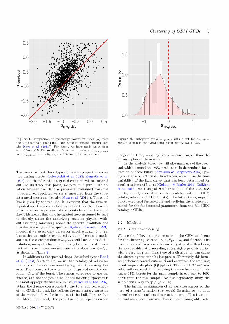
Figure 1. Comparison of low-energy power-law index (α) from

the time-resolved (peak-flux) and time-integrated spectra (see

also Nava et al. (2011)). For clarity we have made an α-errorcut of ∆α < 0.5. The medians of the uncertainties on αintegratedand αresolved, in the figure, are 0.09 and 0.19 respectively

.

The reason is that there typically is strong spectral evolu-tion during bursts (Golenetskii et al. 1983; Kargatis et al.1995) and therefore the integrated emission will be smearedout. To illustrate this point, we plot in Figure 1 the re-lation between the Band α parameter measured from thetime-resolved spectrum versus α measured from the time-integrated spectrum (see also Nava et al. (2011)). The equalline is given by the red line. It is evident that the time in-tegrated spectra are significantly softer than then time re-solved spectra, since most of the points lie above the equalline. This means that time-integrated spectra cannot be usedto directly assess the underlying emission physics, with-out assuming something about the spectral evolution andthereby smearing of the spectra (Ryde & Svensson 1999).Indeed, if we select only bursts for which αresolved > 0, i.e.bursts that can only be explained by thermal emission mech-anisms, the corresponding αintegrated will have a broad dis-tribution, many of which would falsely be considered consis-tent with synchrotron emission since the slope is α <−2/3,as shown in Figure 2.

In addition to the spectral shape, described by the Bandet al. (1993) function fits, we use the catalogued values forthe bursts duration, measured by T90, and the energy flu-ence. The fluence is the energy flux integrated over the du-ration, T90, of the burst. The reason we choose to use thefluence, and not the peak flux, is that for our purposes it isthe most appropriate measure to use (Petrosian & Lee 1996).While the fluence corresponds to the total emitted energyof the GRB, the peak flux reflects the momentary variationof the variable flow, for instance, of the bulk Lorentz fac-tor. More importantly, the peak flux value depends on the

0.0

0.5

1.0

1.5

−1 0 1αintegrated

De

nsity

Figure 2. Histogram for αintegrated with a cut for αresolvedgreater than 0 in the GBM sample (for clarity ∆α < 0.5).

integration time, which typically is much larger than theintrinsic physical time scale.

In the analysis below, we will also make use of the spec-tral width around the νFν peak, that is determined for afraction of these bursts (Axelsson & Borgonovo 2015), giv-ing a sample of 689 bursts. In addition, we will use the timevariability of the light curve, that has been determined foranother sub-set of bursts (Golkhou & Butler 2014; Golkhouet al. 2015) consisting of 804 bursts (out of the total 938bursts, we only used the ones that matched with our GBMcatalog selection of 1151 bursts). The latter two groups ofbursts were used for assessing and verifying the clusters ob-tained for the fundamental parameters from the full GBMcatalogue GRBs.

2.2 Method

2.2.1 Data pre-processing

We use the following parameters from the GBM cataloguefor the clustering searches: α, β,Epk, T90, and fluence. Thedistributions of these variables are very skewed with β beingthe most problematic, revealing a Rayleigh type distributionwith a very long tail. This type of a distribution can causethe clustering results to be less precise. To remedy this issue,we performed several cuts on β and examined the resultingquantile-quantile plots (QQ-plots). The cut at β >−4 wassufficiently successful in removing the very heavy tail. Thisleaves 1151 bursts for the main sample in contrast to 1692burst from the raw sample. We also separately study thesample with very steep β (β <−4).

The further examination of all variables suggested theneed of a transformation that would Gaussianize the databy gathering the outliers closer to the mean. This is an im-portant step since Gaussian data is more manageable, with

MNRAS 000, 1–?? (2017)

4 Z. Acuner et al.

intuitive mean and median results, furthermore, normalityis a requirement for the clustering method Gaussian Mix-ture Models (GMM) used in this paper. To achieve this, wehave made use of the Box-Cox transformation (Box & Cox(1964)) implemented in the R package forecast (Hyndman& Khandakar 2008). This method both quantifies the devi-ations from Gaussianity in the data as well as later takesthis numerical quantity as an input for producing the trans-formed versions of the variables and hence is more tailoredto the specific data set at hand compared to a plain logarith-mic transformation. Since neither logarithmic nor Box-Coxtransformation can deal with negative data sets, appropri-ate constants were added to the variables with negative val-ues before carrying out this step. The resulting transformedvariables were examined with QQ-plots once more, to iden-tify any significant outliers that may distort the clustering.Following this, the sample was scaled and centered by mak-ing use of the R function scale (R Core Team 2013) whichincludes subtracting the mean of the parameter from everyelement and diving them by the standard deviation. This iscarried out so that the features which have broader range ofvalues do not dominate the overall variability in the data.

Before feeding the data into different clustering meth-ods, we have performed a principal component analysis(PCA) via the R package factoMineR (Le et al. 2008) to beable to reduce our highly dimensional multivariate data setto a lower-dimensional set. This allows being able to selectthe most dominant components in the data, while removingstrong inherent correlations that might affect the clusteringresults.

2.2.2 Clustering

After the pre-processing, the data was fed into the GaussianMixture Model implementation mClust (Fraley & Raftery2002) in R. GMM provided a feasible background of infor-mation for interpretation of the results since it is modelbased and hence can give probabilities for each burst be-longing to each group. The clustering was performed withselected non-parametric and density based clustering algo-rithms as well and the results were found compatible withthose given by GMM. The number of clusters were deter-mined by the Bayesian Information Criterion (BIC) imple-mented in the Expectation Maximization (EM) algorithmin mClust which assessed the optimal number of clusters.Output of this method was 5 GMM clusters with differentcluster sizes.

The resulting clusters were evaluated by calculating theSilhouette scores with the method silhouette (Rousseeuw1987) in the package cluster (Maechler et al. 2017). Withthis method, we were able to single out the bursts that wereassigned to the wrong clusters during the initial GMM clus-tering. By re-assigning these bursts to their correct clusters,we were further able to improve the Silhoutte scores and theprecision of the clusters at hand.

2.2.3 Spectral analysis of representative bursts

Understanding the spectral morphological specifications ofthe different classes of bursts that are revealed by the clus-tering procedure is the primary goal of this study. The clus-tering analysis is based on the standard spectral fits by using

the Band function. However, the actual spectrum might notbe best described by a Band function.

For understanding the details of each cluster, we havecreated shortlists which are presented in Appendix B witha selection criterion that maximizes the probability of be-longing to a group while minimizing the error on variable αto ensure good convergence of the Band fit in the catalogvalues. The top bursts from these shortlists were analysedspectrally.

To carry out this task, we work with the data from theGamma-ray Burst Monitor (GBM; Meegan et al. (2009) ) onboard the Fermi Gamma-ray Space Telescope. GBM harbors12 sodium iodide (NaI) detectors that observe between 8 keVand 1 MeV as well as two Bismuth Germanate (BGO) detec-tors which are sensitive to a higher energy range of 200 keVto 40 MeV. We use the time-tagged event data (tte) and thestandard response files as provided by the GBM team. Weuse the source and background intervals given in the GBMcatalogue for consistency with the Band fit parameters. Forthe analysis, we use Xspec spectral fitting package (Arnaud1996) and we produce the PHA files to be used in Xspec viagtBurst (Vianello 2016). To be able to assess a large range ofdifferent spectral shapes, we use 8 different empirical spec-tral models: (i) the Band function, (ii) the Band functionand a powerlaw, (iii) the Band function and a blackbody,(iv) the compTT model, which is an analytic model that de-scribes the Comptonization of soft photons in a hot plasma(Titarchuk 1994), (v) a doubly broken powerlaw model witha parameter to adjust for the smoothness of the breaks (de-fined in 6), (vi) a single blackbody, (vii) a blackbody and apowerlaw, (viii) two blackbodies and finally, (ix) two black-bodies and a powerlaw. With these models, we were able toprobe the number of breaks in each spectra, as well as the ex-istence of an additional powerlaw component. We point outthat these models are used to empirically assess the shapeof the spectra and a thorough physical modelling is laterneeded for the interpretation of the radiation mechanisms,such is done in Iyyani et al. (2015); Ahlgren et al. (2015);Vurm et al. (2011); Vianello et al. (2017).

3 CLUSTERING RESULTS OF MAIN SAMPLEβ > −4

The PCA analysis shows that the main variability in thedata set is from Epk, fluence and T90 which drive the clus-tering (Figure 3). The selection of two primary PCA compo-nents for clustering, which explain 63 per cent of the variancein the data, neatly reduces the number of clusters to threewhich is in accordance with the main groups of fluence andT90 that were described in Section 1. However, since thisstudy strives for an explanation of spectral morphology, weuse all 5 components for the clustering to make use of themore minor variability in parameters α and β which resultsin 5 GMM clusters. The final result of the clustering anal-ysis is given in Table 1 with values of variables used in theclustering for each cluster. These properties are clearly dis-tinguished between the groups and the most notable are thelarge Epk values in clusters 2 and 5 and the short durationsin cluster 5.

MNRAS 000, 1–?? (2017)

Clustering of GBM GRBs 5

Table 1. The list of samples sizes, means, standard deviations (SD), medians and inter-quantile ranges (IQR) for the five variables used

in the clustering for five GMM clusters.

Cluster ID Sample size Band parameters (mean(SD), median, IQR)

Epk [keV] α β Fluence [erg/cm2] T90[s]

Cluster 1 369 139(85), 206, 86 -0.36(0.67), -0.48, 0.6 -2.9(0.4), -2.8, 0.7 7(9), 4, 6×10−6 31(39), 19, 27

Cluster 2 381 503(616), 645, 345 -0.74(0.31), -0.77, 0.4 -2.4(0.4), -2.3, 0.5 3(6), 1.5, 3×10−5 76(94), 47, 71

Cluster 3 233 94(72), 118, 79 0.44(1.42), -0.05, 1.5 -1.9(0.2), -1.9, 0.3 3(3), 2, 2×10−6 35(49), 24, 35

Cluster 4 40 242(377), 323, 141 -1.47(0.14), -1.43, 0.2 -2.4(0.6), -2.2, 0.9 5(7), 2, 6×10−6 36(79), 37, 51

Cluster 5 128 604(664), 144, 588 0.7(2.82), -0.09, 1.2 -2.3(0.6), -2.2, 0.8 8(0.1), 4, 5×10−7 1.1(1.4), 0.54, 0.06

α β

Epk

T90

Fluence

−1.0

−0.5

0.0

0.5

1.0

−1.0 −0.5 0.5 1.0

Dim

2 (2

4.6%

)

Variables factor map − PCA

30

40

50

60

70

80

Contrib.

0.0Dim1 (38.3%)

Figure 3. Contributions of the five variables to first (x-axis) andsecond (y-axis) PCA dimensions represented inside the circle of

correlations.The percentage of total contribution is given by the

color coding and the angles to the two axes are indicative of thepercentage of contributions to either dimension.

3.1 Appearances in 2D plots

Before examining each cluster in more detail, it is interestingto asses them in different parameter spaces (Figures 4 to 10)selected for their representative powers compared to otherpairings. Note that the primary focus of this study is not tostudy correlations between observed quantities, but ratherto identify classes of burst with different properties. Never-theless, the two-dimensional plots are useful in illustratingwhere the different clusters dominate.

Figure 4 presents the GMM clusters in log(T90) versuslog(Fluence). Apart from the distinct cluster 5 (low fluence,small T90; orange in Fig. 4) there is only a very weak cor-relation (coefficient of determination R ∼ 0.4; correlationcoefficient ∼ 0.64). However, the remaining clusters do oc-cupy different regions distinguished by fluence. In particu-lar, we note that cluster 2 (blue) distinguishes itself from the

low fluence clusters (green, red, purple). The Kolmogorov-Smirnov test rejects the hypothesis of these two groups beingthe from the same distribution with a p−value smaller than2.2× 10−16.

Figure 5 presents the GMM clusters in log(Epk) versusα. For plotting purposes alone, we cut the α-axis at α = +2.The reason is that, first, this is the hardest slope expectedtheoretically since it is the sub-peak slope of a Wien spec-trum. Second, all bursts with a measured value of α > 2(46 bursts), have large measurement errors and all are infact consistent with the Rayleigh-Jeans’ slope of α = 1, towithin one sigma. Note also that the GBM detector hasa limited energy range, which imposes a restriction in therange of Epk. In the figure, one can see a division inside thegroup of long bursts from Epk ≈ 400 keV, where the clus-ters 2 (blue) remains at the high Epk side while clusters 1(red) and 3 (green) have lower Epk values. The short bursts,cluster 5 (orange), have high overall Epk values around thesame range with cluster 2 while cluster 4 (purple) has aintermediate range of Epks.

Figure 6 presents the GMM clusters in log(Epk) ver-sus log(Fluence). Cluster 2 is gathered in the region of highfluences and high peak energies, while the other extreme,cluster 3, is gathered at low Epk values and low fluences.The rest of the sample is gathered at intermediate fluencevalues and intermediate Epk values. The exception is theshort burst cluster 5, which has very low fluences but com-parably high Epks. This plot can be compared to figure 1 inNava et al. (2008), which however only includes long burst,that is, cluster 5 does not appear in their figure.

In Figure 7, we plot log(T90) and α values. Cluster 5 isstrikingly apart from the rest of the clusters thanks to itsvery short T90 average. It is seen that clusters 1 and 3 haveshorter T90s and harder αs compared to the longer bursts(clusters 2 and 4).

Figures 8 and 10 depict the relationship of β to Epk andfluence, respectively. It is seen that the short burst clusterhas the lowest fluences and highest (together with cluster2) Epks as well as cluster 3 is very localized in the β rangewith always lower Epk and fluence values than the rest ofthe long burst clusters.

Figure ?? displays the same parameters for Figures 5and 7 but for the 50 bursts that belong to their clusters withhighest probabilities assigned by the GMM. This provides amore concise view of how the clusters are separated.

MNRAS 000, 1–?? (2017)

6 Z. Acuner et al.

−1

0

1

2

3

−7 −6 −5 −4log10(Fluence)

log 1

0(T90

)

Cluster ID12345

Figure 4. Plot of log(T90) versus log(fluence) with color coding

representing the five GMM clusters. The medians of the uncer-tainties on T90 and fluence are 1.9 seconds and 5×10−8 erg/cm2

respectively.

1

2

3

−1 0 1 2α

log 1

0(Epk

)

Cluster ID12345

Figure 5. Plot of log(Epk) versus α with color coding represent-

ing the five GMM clusters. The medians of the uncertainties onEpk and α are 46.6 keV and 0.3 respectively.

3.2 Properties of bursts in the five clusters

Based on the results in Table 1, and alternatively in thefigures above, the property character of the clusters can beidentified.

As mentioned in the previous section, there exists twomain categories defined by T90 and separates the long(T90>2) and short bursts (T90<2) that have long been ac-knowledged as two distinct classes of bursts (Kouveliotouet al. 1993). Furthermore, we detect the existence of twodifferent type of long bursts that are separated as high andlow fluence bursts (§3.1). These results are in accordancewith previous studies that were focused on BATSE data (seeand §1). With the addition of the spectral parameters intothe parameter space, we obtained a novel classification that

1

2

3

−7 −6 −5 −4log10(Fluence)

log 1

0(Epk

)

Cluster ID12345

Figure 6. Plot of log(Epk) versus log(fluence) with color coding

representing the five GMM clusters. The medians of the uncer-tainties on Epk and fluence are 46.6 keV and 5×10−8 erg/cm2

respectively.

−1

0

1

2

3

−1 0 1 2α

log 1

0(T90

)

Cluster ID12345

Figure 7. Plot of log(T90) versus α with color coding representingthe five GMM clusters. The medians of the uncertainties on T90and α are 1.9 seconds and 0.3 respectively.

combines the intrinsic and extrinsic properties of GRBs withclusters that both describe the spectral morphologies as wellas the fluence and overall length of the bursts.

Now we are in a position to outline a general descriptionof the burst sample at hand. There exists five clusters:

(i) long bursts with low fluence values and narrow spec-tra consisting of short minimum variability time scales (clus-ter 1),

(ii) very long bursts with high fluence values that con-sists of very short minimum variability time scales (cluster2),

(iii) intermediate length long bursts with very broadspectra and very long minimum variability time scales (clus-ter 3),

MNRAS 000, 1–?? (2017)

Clustering of GBM GRBs 7

−7

−6

−5

−4

−4 −3 −2β

log 1

0(Flu

ence

)

Cluster ID12345

Figure 8. Plot of log(fluence) versus β with color coding repre-

senting the five GMM clusters. The medians of the uncertaintieson T90 and fluence are 5×10−8 erg/cm2 and 0.4 respectively.

1

2

3

−4 −3 −2β

log 1

0(Epk

)

Cluster ID12345

Figure 9. Plot of log(Epk) versus β with color coding represent-

ing the five GMM clusters.The medians of the uncertainties onEpk and β are 46.6 keV and 0.4 respectively.

(iv) intermediate length long bursts with broad spectraand long minimum variability time scales (cluster 4),

(v) short bursts with very low fluence that have veryshort minimum time scale variabilities which can fundamen-tally be described by a single narrow component (cluster 5).

To further illustrate the differences between the clus-ters we plot in Figure 11 the α-distributions as violin plots.Even though the α-parameter only contains minor variabil-ity in the data set (§3.4), and therefore is not dominant informing the clusters, a clear distinction in α-distributions isapparent. In particular, while clusters 2 and 4 are heavily oc-cupying the α < 0 region, clusters 1, 3 and 5 span the regionbetween α = 0 to α = 1 as well, where only photosphericemission can reside (see further discussion in §5.1).

In Section 3.3, we discuss the properties of each groupin more detail in the light of the parameters summarized

1

2

3

−2 −1 0 1 2α

log 1

0(E p

k) Group ID12345

−1

0

1

2

3

−2 −1 0 1 2α

log 1

0(T9

0) Group ID12345

Figure 10. Plots of log(Epk) versus α (cf. Fig. 5) and log(T90)

versus α (cf. Fig. 7) for only the top 10 most probable bursts

within each cluster, with color coding representing the five GMMclusters. The clusters now appear more distinctly.

in Tables 1 and 2. In Section 4.1, we discuss the spectralmorphologies of each group independent of the Band fit pa-rameters from the GBM catalog that were used to clusterthe sample. Finally, in Section 4.2, we propose a parameterto probe the temporal characteristics of GRBs which is laterused to narrate the temporal morphology of each group.

3.3 Characteristics of the clusters in terms ofBand parameters

3.3.1 Cluster 1

Cluster 1 has an average α value of -0.36, which suggestsa mediocre low energy powerlaw indice compared to otherclusters. The sample size is quite large with 369 bursts andthis cluster has the second highest fluence average among theclusters while having an Epk average of ≈ 140 keV whichis the second lowest observed. T90 averages approximatelyaround 30 seconds with the minimum time scale variabilitybeing around 1 second.

MNRAS 000, 1–?? (2017)

8 Z. Acuner et al.

3.3.2 Cluster 2

Cluster 2 has the largest sample size of all groups with 381bursts. This cluster has the second highest average Epk with≈ 500 keV and a soft average low energy index, α with ≈-0.7. It has the highest fluence average among our clusters.T90 averages approximately at 70 seconds that indicates thelongest bursts are gathered in this cluster which show a quitehigh variability in time with an average ∆tmin of ≈ 0.3seconds.

3.3.3 Cluster 3

Cluster 3 has the lowest average Epk value at ≈ 90 keV aswell as the second lowest average fluences with an α averageof 0.5. This cluster has an intermediate T90 average whichapproximates to 35 seconds. The average ∆tmin for Cluster3 is ≈ 2 seconds, which makes the bursts in this group oneof the least variable ones among the GBM cluster sample.This group is moderately populated with 233 members.

3.3.4 Cluster 4

The 4th cluster is the least populated cluster in our samplewith 40 bursts. This cluster has an average Epk of ≈ 240keV with a very soft α average (≈ -1.5). The fluence andT90 (≈ ave. 40 seconds) are quite moderate with a ∆tmin of≈ 2 seconds.

3.3.5 Cluster 5

Cluster 5 has the highest Epk average at ≈ 600 keV as wellas the hardest average α value of ≈ 0.7 which suggests thatthis cluster is mainly dominated by bursts with very ther-mal spectra. However, the median α of the cluster is ≈ 0 soabout half of the bursts exhibit negative low-energy indices.The cluster has the lowest fluence average which is mainly aconsequence of its very low T90 average of ≈1 seconds. Dueto the strikingly short T90 values of the bursts occupyingthis cluster, we identify Cluster 5 as consisting of the mainmajority of short bursts in our GBM sample. Indeed, whileClusters 1 to 4 have a total of 10 bursts that have T90 <2, Cluster 5 has 121 bursts (out of a total of 128) that fallinto the short burst category. Another property that dis-tinguishes this cluster from the others is its highly variablelightcurve, with a minimum variability time scale average of≈ 0.2 seconds which is the lowest among all clusters.

3.4 Clustering results of main sample β < −4

The methods used in the clustering analysis above, requirethe parameter distributions to be Gaussian. Since the β dis-tribution is highly skewed we had to make a cut at a largevalue of β = −4. We note that values less than −4 repro-duces spectra that remain relatively similar, and all thesebursts are close to having a exponential cutoffs. Neverthe-less since the sample with β < −4 contains 541 bursts of theinitial 1692 in our studied sample, we analyze it separatelyand compare the results with that of the main sample.

From this sample, six clusters were extracted followingthe method of Section 2.2. Clusters in this sample emergeas the branches of the classes labeled as single break in the

−2

−1

0

1

2

1 2 3 4 5Group ID

α

Figure 11. Distribution of α-values for the five clusters shown

as violin plots.

main sample (clusters 2 and 4 mostly). All 6 clusters havevery soft α means with the softest being ≈ -1.7, belonging toa cluster that contains characteristically very broad spectrawith high-energy, exponential cut-offs. The short bursts areagain picked up by the clustering method in a single cluster,however, these have Epk values a few times higher than thatof cluster 5 of the main sample. T90, Epk, and to a lesserextent α, seem to be the major drivers of the variance inthis sample.

4 FURTHER ANALYSIS OF CLUSTERPROPERTIES

In this section, we further examine the properties of thebursts in the different clusters.

Characteristics of the clusters which were not used inthe clustering but nevertheless are helpful in interpretingthe cluster are presented in two tables. Table 2 includes theminimum variability time scale, ∆tmin, the smoothness pa-rameter, S, defined in eq. (1), and spectral width, while Ta-ble 3 includes the redshift, isotropic energy (Eiso), and thepeak flux at 64 ms.

4.1 Spectral morphology of each cluster

In this section, we perform detailed spectral analysis on thebursts that belong to their respective clusters with the high-est probabilities, as described in §2.2.3.

4.1.1 Cluster 1

From the examination of its bulk Band parameter valuesgiven in the previous section, Cluster 1 can be identified witha non-thermal spectral appearance (Figure 12). Indeed, inthe spectral analysis of the template bursts for this cluster,

MNRAS 000, 1–?? (2017)

Clustering of GBM GRBs 9

Table 2. The list of means, standard deviations (SD), medians and inter-quantile ranges (IQR) for three external parameters that are

used in the interpretation of the five GMM clusters. Here ∆tmin is the minimum time scale variability, the smoothness parameter S isdefined in eq. 1, and spectral width.

Cluster ID External parameters (mean(SD), median, IQR)

∆tmin [s] S Width

Cluster 1 0.98(1.27), 0.48, 1.08 0.2(0.1), 0.2, 0.1 1.04(0.35), 1.12, 0.4

Cluster 2 0.86(1.65), 0.34, 0.78 0.02(0.07), 0.02, 0.06 1.7(0.9), 1.3, 0.9Cluster 3 2.02(3.68), 0.83, 1.98 0.1(0.2), 0.1, 0.2 2.8(1.4), 2.5, 2

Cluster 4 1.71(1.66), 1.15, 1.61 0.08(0.09), 0.05, 0.2 2.3(1.4), 1.6, 1.1

Cluster 5 0.16(0.42), 0.03, 0.06 0.2(0.2), 0.08, 0.2 1.29(0.78), 1.02, 0.6

Table 3. The list of means, standard deviations (SD), medians and inter-quantile ranges (IQR) for three burst parameters that are used

in the interpretation of the five GMM clusters. ”NA” symbol stands for cluster parameters for which no Eiso calculation was possible

due to a lack of adequate number of bursts with measured redshift.

Cluster ID External parameters (mean(SD), median, IQR)

Redshift Eiso [erg] Peak flux [pht/cm2.s]

Cluster 1 1.68(0.92), 1.69, 1.46 3(5), 0.9, 2×1053 15(22), 5, 11

Cluster 2 1.57(0.82), 1.64, 0.8 3(4), 1, 5×1053 27(67), 27, 17

Cluster 3 2.48(1.21), 2.1, 1.92 2(3), 0.5, 0.4×1053 3(4), 5, 3Cluster 4 0.71(NA), 0.71, NA 3(NA), 3, NA×1052 7(5), 6, 2

Cluster 5 NA(NA), NA, NA NA, NA, NA 13(18), 8, 8

11

01

00

10

00

10

4

ke

V2 (

Ph

oto

ns c

m−

2 s

−1 k

eV

−1)

NaI 8NaI B

BGO 1

10 100 1000 104

−1

00

10

20

no

rma

lize

d c

ou

nts

s−

1 k

eV

−1

Energy (keV)

Figure 12. Cluster 1 template burst, GRB100816024, fitted withthe Band function.

it is seen that the PGStat value has the largest reduction forthe Band function. This cluster is characterized by a singlesmoothly broken powerlaw which is narrower compared toClusters 2 and 4 which are also best described with thismodel. The Epk has a modest value generally around a fewhundred keVs and the fluences are also modest, comparedto Cluster 2. Cluster 1 averages the second highest peak fluxand a high isotropic energy (Eiso) output (refer to Table 2).

4.1.2 Cluster 2

Cluster 2 has softer low energy index values than Group1 for the catalogue Band fits, which reflects itself in ourspectral analysis as well (Figure 13). A significant amount

11

01

00

10

00

10

4

ke

V2 (

Ph

oto

ns c

m−

2 s

−1 k

eV

−1)

NaI 2NaI 5

BGO 0

10 100 1000 104

−1

00

10

20

no

rma

lize

d c

ou

nts

s−

1 k

eV

−1

Energy (keV)

Figure 13. Cluster 2 template burst, GRB12071115, fitted withthe Band function.

of improvement in the fit is obtained when these spectra aredescribed with a Band function, as compared to the othermodels tried. This cluster is also described by a single breakand a wide spectrum and it contains the brightest bursts inour sample which is evident from its high Eiso and peak fluxaverage values.

4.1.3 Cluster 3

The bursts in Cluster 3 are very rich in spectral features,which clearly distinguishes them from the rest of the sam-ple (Figure 14). The best fit model is perceived to be twoblackbodies from the comparison of PGStat values with anoccasional need for an additional powerlaw component. The

MNRAS 000, 1–?? (2017)

10 Z. Acuner et al.1

10

10

01

00

01

04

ke

V2 (

Ph

oto

ns c

m−

2 s

−1 k

eV

−1)

NaI 1

NaI 3

BGO 0

10 100 1000 104

−4

−2

02

no

rma

lize

d c

ou

nts

s−

1 k

eV

−1

Energy (keV)

Figure 14. Cluster 3 template burst, GRB091215234, fitted withtwo blackbodies.

110

100

1000

10

4

keV

2 (

Photo

ns c

m−

2 s

−1 k

eV

−1)

NaI 2NaI 1

BGO 0

100 1000 104

−5

05

norm

aliz

ed c

ounts

s−

1 k

eV

−1

Energy (keV)

Figure 15. Cluster 4 template burst, GRB100517072, fitted with

the Band function.

main spectral shape that is being captured with two black-bodies is a double break spectrum with a non-flat featurein between the two breaks. This kind of a spectral featurein between the lower and higher energy breaks is what givesthese spectra a quite ”wiggly” appearance. Cluster 5 alsocontains the second hardest α values which are captured bythe blackbody fits. Members of this cluster tend to be quitefaint with low peak flux averages.

4.1.4 Cluster 4

Cluster 4 is found to be best described with a Band modelas Groups 1 and 2 but it exhibits quite a different spec-tral shape with a characteristic weak break at high energiesand very flat low energy power-law indices, producing muchbroader spectra (Figure 15). There are occasional fluctua-tions at energies lower than 20 keV, which could be inter-preted as a break, however features at these energies areaffected by the lower effective area of the instrument andhence, analysis only including higher energies are preferredfor this cluster. The group distinguishes itself from Clusters1 and 2 by its very low peak flux averages as well and theEiso is also low for this cluster.

11

01

00

10

00

10

4

ke

V2 (

Ph

oto

ns c

m−

2 s

−1 k

eV

−1)

NaI BNaI A

BGO 1

10 100 1000 104

−1

00

10

20

no

rma

lize

d c

ou

nts

s−

1 k

eV

−1

Energy (keV)

Figure 16. Cluster 5 template burst, GRB100805300, fitted with

a single blackbody.

4.1.5 Cluster 5

Among our clusters, Cluster 5 has the most extreme proper-ties concerning the low energy power law index, T90 as wellas the minimum variability time scale. This is strongly re-flected in the spectral analysis of the 10 most probable burstsin this cluster, which can be well described by a single nar-row spectral component with a very steep low energy index,namely a blackbody or a broadened blackbody that can becaptured by a smoothly broken power-law such as the Bandfunction or a multicolor blackbody (Figure 16). We note,however, that these 10 top probability bursts, with a me-dian of 0.25, are harder than the full sample, which has amedian around 0. Many bursts in this cluster therefore haveα < 0 which should be taken into account when consideringthe general properties of cluster 5 (see Section 5 for moredetails). There is no information on Eiso due to the lack ofmeasured redshifts for this cluster, although its peak fluxaverages are comparable to that of clusters with brighterbursts.

4.2 Temporal morphology of each group

GRB light-curves are very various in their appearances.This seemingly chaotic behavior is possibly stemming fromvery many distinct processes contributing to the shaping ofthe light-curves that are observed. Dentangling each one ofthem is deemed to be a daunting process, however a usefulone in understanding the spectral properties better. Here,we attempt to at least classify some of the very abundantlightcurve behaviors depending on their temporal character-istics. We start this task by defining a smoothness parameter(S) for the temporal morphology of a GRB,

S =∆tmin/T90

σx, tmin(1)

where ∆tmin is the minimum time scale variability andσx, tmin is the fractional flux variation level at ∆tmin asinvestigated in Golkhou et al. (2015).

Defined this way, the smoothness parameter is able tocapture the appearance of time variability over the range ofT90, taking into account how significant the fluctuations dur-ing ∆tmin is by taking into account σx, tmin. A low value of

MNRAS 000, 1–?? (2017)

Clustering of GBM GRBs 11

the smoothness parameter indicates a light-curve with manypeaks or one heavily variable peak that may look damped.Larger smoothness parameters indicate a burst with a sin-gle, smooth pulse that can be interpreted with a simplertemplate. For a decent assessment of the light-curves withthis measure, a model independent peak flux cut is required,which we determined as the peak flux on 64 ms timescalebeing larger than 5 photons cm−2s−1 as a minimum. Burststhat fall below this flux cut are occasionally too low in countsand hence, give little understanding of how these three pa-rameters work to produce each distinct light curve. This iswhy both fluence values used in the clustering and peak fluxvalues are given in Tables 1 and 3. Fluences are used in theclustering to be able to capture the full energetics of thebursts and for the convenience of being able to compare theresults with the previous studies which used fluences. It isworth mentioning however that we have verified the robust-ness of the clustering results by doing the clustering for peakfluxes as well.

The variability measures are given in Table 2 and con-clusions are drawn in §5.3.

4.3 Redshift distribution and fluence biases

Most of the bursts used in the clustering analysis do nothave measured redshift. For the 27 bursts (9, 12, 5, 1, and0 in each cluster, respectively) that have values we can as-sess the median redshift for the different clusters (see Table2). However, since the number is small any firm conclusioncannot be drawn.

The lack of knowledge of the redshift will propagate intoan added dispersion of measured quantities of Epk, T90, andfluence. Perley et al. (2016) find the redshift distribution ofGRBs to mainly be in the range of 0.6 < z < 4.0, peakingin the range 1.5 < z < 2.5 (see also, e.g., Le & Mehta(2017)). The observed values of Eobs

pk = E′(1 + z)−1, whereE′ is the peak energy in the progenitor rest frame, whichthus translates into a dispersion of a factor of 3 (factor of1.4 for the peak in the z-distribution). This is much smallerthan the observed dispersion of Eobs

pk (seen in, e.g., Fig. 6).For the duration, one would expect T90 = T ′90(1 + z)1−a,where a ∼ 0.5 is the intrinsic dependence of the duration onthe photon energy (Fenimore et al. 1995; Lee & Petrosian1997), leading to a dispersion of 1.4 (1.8 for the bursts inthe distribution peak). Indeed, Kocevski & Petrosian (2013)concluded that any time dilation effect is masked by intrinsicand instrumental effects. Finally, for the fluence F = ε(1 +z)/4π d2L, where ε is the total energy and dL is the luminositydistance (Petrosian & Lee 1996; Meszaros et al. 2011) . Thisleads to a dispersion of a factor of 33 (2.5 for the peak range),which again is smaller than the observed dispersion (Fig. 4).However, this dispersion is of the size of the dispersions ofthe individual clusters. Indeed, all the effects of the unknownredshifts will lead to a fuzziness in any clustering of burstsproperties, most noticable in the value of the fluence.

We also point out that bursts that are intrinsicallyweak, for instance due to large redshift or due large view-ing angles, might only be partly detected by the GBM. If asignificant fraction of the burst emission is lower than theinstrument background level, then only part of the durationand the fluence will be measured. This could introduce a biastowards short and low fluence bursts. This should, however,

only affect the weakest bursts, that are close to the detectionthreshold of the instrument (Kocevski & Petrosian 2013). Inaddition, the dispersions in fluence and T90 of strong burstsare large, as can be seen in Figure 4. Assuming that thesedispersions reflect the intrinsic dispersions, also valid for theweakest bursts, then the effects of such a biases are not ex-pected to be dominant.

5 DISCUSSION

The main question that we want to answer is if there isevidence for clustering of burst properties and if this cangive hints to whether there is a single or multiple emissionprocesses involved.

There are a number of effects that is expected to smearour any distinct clusters. First, we rely on Band functionfits. In some cases, the underlying physical spectrum mightbe different. In such cases the Band parameters are only aproxy of the actual shape. Second, as mentioned in §4.3, theunknown redshift will add additional dispersion. Third, itshould also be noted that since we are only considering thespectrum of the light curve peak, any evolution of the typeof spectrum is not captured. For instance, the ratio of thethermal and non-thermal component can vary through outa burst (discussed below in §5.4). It can also be imaginedthat a purely thermal burst transitions into a synchrotronburst and vice versa (e.g. Guiriec et al. (2013), Zhang etal. arXiv:1612.03089). Due to all these effects, we thereforeonly expect marginal evidence of clustering from the pa-rameters distributions alone. We note, however, that in asimilar study on BATSE bursts, five cluster were also iden-tified based on fluence, duration and spectral information,supporting the statistical result for the clustering (Chat-topadhyay & Maitra 2017).

If the clustering, that we determine, is due to differentemission processes involved, the properties of the differentclusters should reflect the particularities of the individualemission processes. By studying the cluster properties fromthe point-of-view of the emission process can thus lend fur-ther support of both the existence, as well as the cause ofthe clustering.

To address this question further, we therefore discussbelow the α-distributions and the time-variability of the fiveclusters identified.

5.1 The α-distribution and emission mechanism

As mentioned in Section 3, the main parameters for the clus-tering are Epk, T90 and fluence (see figure 3). It is there-fore noteworthy that the five clusters do have different α-distributions despite of the fact that α had little impact inidentifying the clusters.

Figure 11 shows the α-distribution for the five groupsand we note that clusters 2 and 4 are conspicuous. First, theyhave exclusive contributions of α < 0, and therefore are con-sistent of being purely non-thermal. At the same time thewidth of the α-distributions are narrower and more symmet-ric than the other groups. Second, we note that these twoclusters comprise the longest bursts, that can be seen by,for instance, from their median T90-values. Third, neglect-

MNRAS 000, 1–?? (2017)

12 Z. Acuner et al.

ing cluster 5, which contain the short bursts, cluster 2 and4 have large Epk-values.

It is therefore suggestive that the peaks and the widthof the α-distributions of cluster 2 and 4 closely match thepredictions made for GBM observations of synchrotron emis-sion (Burgess et al. 2014). They showed that the observeddistribution should have narrow peaks at −0.8 and −1.5.The narrowness for clusters 2 and 4 is remarkable, takinginto account the measurement errors on α as well as thepossibility of bursts being wrongly assigned to each clus-ter, which would all increase the width of the distribution.Therefore, it can easily be argued that these two clusters aredominated by bursts that are due to synchrotron emission.Moreover, since synchrotron emission is expected to give abroader dispersion in Epk compared to photospheric emis-sion, the observed broadness of the Epk distribution sup-ports this interpretation for above mentioned clusters. Thereason to expect a broader Epk distribution is that, for syn-chrotron, Esynchpk ∝ γ2

elΓB⊥, where γel is the typical electronLorentz factor, Γ is the bulk Lorentz factor, and B is thetypical magnetic field strength. Variations in any of theseparameters will naturally cause a dispersion. On the otherhand, photospheric emission is expected to have quite nar-row peak energy distributions (Beloborodov 2013; Vurm &Beloborodov 2016).

It is important to bear in mind that in the clusteringanalysis above we only use one time-resolved measurementof α per burst: The peak-flux value. In order to properlyassess the emission mechanism during a burst obtaining thefull spectral evolution is desirable. To further examine thebehaviour of bursts in cluster 2 (the most populated), wetherefore examined the time-resolved evolution of α withinthe most probable bursts within the cluster. We find thatα stays within the expected range for synchrotron emission.We illustrate this on GRB130606 which is assigned to clus-ter 2 with high significance and has a α = −0.68 at the lightcurve peak (this is the value used for the clustering study).Figure 17 shows the α and light curve of this burst. Themain point to note here is that the spectra varies over theburst, there is spectral evolution. We note that the burst isconsistent with synchrotron emission throughout the evolu-tion, but the α value changes from ∼ −0.7 to ∼ −1.5, thatis, from the slow to fast cooling regimes. Another way of as-sessing the range of α-values that occur during a burst is tostudy the time-integrated spectrum. The averaged value ofthe time-integrated α-value for the 5 most probable bursts incluster 2 is < α >= −1.002, which is well within the allowedrange for synchrotron emission.

We will therefore denote this group the synchrotrongroup, since it is dominated by bursts with properties thatare consistent with synchrotron emission. The group con-sists of bright, long bursts, with a single spectral peak, andcontains 37 % of the bursts in the analysed sample.

The three remaining clusters (1, 3, and 5), on the otherhand, do still have a significant fraction of bursts that haveα > 0. It can therefore be argued that many of the burstsmust have been produced through a photospheric mecha-nism, such as subphotospheric dissipation. One could, how-ever, also imagine that these groups contain bursts froma mixture of emission mechanisms, some synchrotron andsome photospheric. However, among the bursts that havebeen assigned to clusters 1, 3, and 5 with a probability

Time [s]

Time [s]

Figure 17. The light curve and α-evolution for the synchrotron

bursts GRB130606. The α varies within the expected values forsynchrotron emission.

larger than 0.8, only 8.5% are consistent with α < −0.8.The vast majority of the bursts are thus inconsistent withsynchrotron emission. We further note that the parameterdistributions of the fluence, Epk, β, and T90 do not vary forbursts with α below and above α = −0.8. This propertyfurther supports the single emission interpretation for themajority of these bursts. We also performed analysis of thetime-resolved spectral evolution within these bursts. This isillustrated by the example in Figure 18, which shows time-resolved data for GRB130220. The peak flux value (used inthe clustering analysis) for this case is α = −0.32. Duringthe bursts α evolves strongly, but is limited in the rangefrom -1 to 1. Similarly, the average < α >-value for thetime-integrated spectra of bursts in cluster 1 can be inves-tigated. For the 5 most probable bursts in cluster 1 the av-eraged value is < α >= −0.586. This value is significantlymuch harder than the corresponding value found for cluster2, given above (−1.002).

From a theoretical point-of-view many spectral shapescan be produced by the photosphere (e.g. Pe’er et al. 2006;Vurm & Beloborodov 2016). The diversity of spectral typesthat can be fitted by photospheric models is illustratedby GRB090618, which was successfully fitted by Ahlgrenet al. (2015), while the Band function fits yield α-values inthe range -0.8 to -1 (Izzo et al. 2012). Another example is

MNRAS 000, 1–?? (2017)

Clustering of GBM GRBs 13

Time [s]

Time [s]

Figure 18. The light curve and α-evolution for the synchrotronbursts GRB130220. The α varies within the expected values for

photospheric emission.

GRB100724B which was fitted by two different photosphericmodels (Ahlgren et al. 2015; Vianello et al. 2017), while theα-values lie in the range of -0.75 to -0.45 (Guiriec et al. 2011;Vianello et al. 2017). This shows that a large dispersion inα-values can be reproduced by photospheric models.

Based on these arguments, we therefore suggest thatthese clusters should form a photospheric group since theyare dominated by bursts that are inconsistent with syn-chrotron emission, but consistent with emission from thephotosphere. The group comprises clusters 1 (dimmer,single-peaked bursts), 3 (multi-break bursts) and 5 (mainlyshort bursts). These group contains a majority of all bursts,namely 63%.

5.2 Photospheric versus synchrotron bursts

Based on the arguments in the previous section, we sug-gest that approximately 1/3 of all bursts are caused by syn-chrotron emission while approximately 2/3 of bursts are dueto emission from the photosphere.

The α-distributions between the synchrotron and thephotospheric groups are significantly different. The two-sample Kolmogorov-Smirnov test gives D = 0.47, while the

2

3

−1 0 1 2α

log 1

0(Epk

)

Cluster ID12

Figure 19. Peak energy (Epk) versus α for cluster 1 (SPD bursts)

and 2 (synchrotron bursts). The α distribution is cut at 2.

Wilcoxon rank sum test with continuity correction gives W= 22, which both significantly reject the hypothesis thatthe two distributions are drawn from the same distribution.Figure 19 shows the two distributions in the α-Epk plane,in which a clearly separation can be seen. To further illus-trate this, in figure 20 the density distribution of α-valuesfor bursts in these two groups are shown. For this plot wehave selected bursts in our sample which have α < 3 and∆α < 1.0, and that have a probability of at least 0.8 tobelong to a cluster. This was done in order to only selectthe bursts with well determined α, and group assignments,since we want to focus on bursts which clearly reveal theiremission spectra. The synchrotron bursts are plotted withthe red curve and the photospheric bursts are plotted withthe green, dashed curve.

It is clear from figure 20 that the synchrotron burstshave two narrow peaks at the expected values. Approxi-mately 20% of the synchrotron bursts are in the fast coolingpeak. In contrast, the photospheric bursts do not have apreferred α-value, but rather have a very broad peak. Wenote that there is a small a peak at α ∼ 0.3, which is closeto the expected value of coasting phase photosphere, whichshould have an asymptotic value of α ∼ 0.4 (Beloborodov2010). Moreover, the photospheric α-distribution appears tobe limited by α = -1 and = 1. The latter distribution is in-deed what is expected for subphotospheric dissipation emis-sion for low magnetised outflows (Pe’er et al. 2006; Vurm& Beloborodov 2016). The hard spectral limit of 1 is theRayleigh-Jeans’ value while the soft spectral limit can be as-signed to the value that is expected from Comptonisation ofa soft synchrotron emission contribution between the Wienzone (at τ ∼ 100) and the photosphere (at τ ∼ 1). Indeed,Vurm & Beloborodov (2016) finds that α = −1 is a naturalvalue to expect in a case of continuous dissipation throughout the jet. A much softer α is only expected in cases withlarge magnetisation.

In figure 21 we plot the α-distribution for all shortbursts (see also Nava et al. (2011)). We select all burstsin our sample that have T90 < 2 s. In comparison we alsoplot the α-distribution of the photospheric bursts identified

MNRAS 000, 1–?? (2017)

14 Z. Acuner et al.

−2.0 −1.5 −1.0 −0.5 0.0 0.5 1.0 1.5

0.0

0.5

1.0

1.5

α

Den

sity

Figure 20. Density distributions of α for two samples: the com-

bination of cluster groups 2 and 4 (red curve), and the combina-tion of cluster groups 1,3 and 5 (green curve). The green curve

represents bursts that have spectra that are interpreted to havea photospheric origin while the red curve represents bursts that

have spectra that are consistent with synchrotron emission.

−2.0 −1.5 −1.0 −0.5 0.0 0.5 1.0 1.5

0.0

0.2

0.4

0.6

0.8

1.0

Den

sity

α

Figure 21. Density distributions of α for two samples: (i) The

photospheric group, clusters 1, 3, and 5 (green, dashed curve)

and (ii) all short bursts in the sample, independent of clusterassignment (red, solid curve).

above (clusters 1,3, and 5). The two distributions cover thesame range, which suggests that the prompt phase in mostshort bursts are due to photospheric emission.

5.3 Time variability and emission mechanism

Further differences between the clusters are summarised inTable 2. It is clear that the synchrotron bursts have morevariable light curves. This is shown by the short ∆tmin aswell as the small value of the smoothness parameter S. Thisresult is consistent with the finding in Dichiara et al. (2016)who found that high Epk bursts tend to be more variableon shorter time scales. In more detail, they found a strongcorrelation between the slope of the power density spectrum(PDS) of the light curve and the Epk values. Since the syn-

chrotron group are characterised by large Epk values, thiscorrelation is consistent with short time variability scale.

Short variability time-scale poses a problem for the syn-chrotron interpretation for these bursts. The reason is thatsynchrotron spectra with α = −2/3 are in the slow-coolingregime, that is, most of the electrons have not had timeto cool below the injection frequency. This sets strong con-straints on the typical energy of the emitting electrons,γel ∼ 105 − 106 (Beniamini & Piran 2013b). This valueis much higher than expected for internal shocks (Bosnjaket al. 2009), which is assumed to explain highly variablelightcurves. However, large γel can be obtained for exter-nal shocks (Panaitescu & Meszaros (1998); Burgess et al.(2016), Duffell & MacFadyen (2015)). In that case the lightcurve variability should be low, due to the large emissionradii. This is in contrast to what is suggested by the dtmin

and PDS measurements.Another way of relaxing the condition of slow cooling

and still maintaining the observed electron distribution is amarginally fast-cooling scenario (Daigne et al. 2011). In sucha case the cooling frequency is close to the minimum injec-tion frequency of the electrons. Indeed, as shown in Figure17, which shows the spectral evolution in GRB130606, thecooling regime indeed seems to vary between fast and slowcooling, which is an indication of a marginally fast-coolingscenario.

Figure 17, also shows that the variability of the lightcurve changes during the burst. It is suggestive that whenα ∼ −0.7 the light curve is less variable. The highly variableperiods 9–10.4 s and 12.5–15.5 s occur during periods α <−2/3. Therefore, the minimum variability time scale neednot occur when the spectrum is in the slow-cooling regime.This alleviates the constraints for synchrotron emission setby the time variability (see further analysis in Acuner et al.2017, in prep.).

5.4 Band + blackbody spectra

One of the models tested for above consisted of a blackbodyin addition to a Band spectrum. Such spectra have previ-ously been successfully fitted to many bursts (e.g. Guiriecet al. 2011, 2013; Iyyani et al. 2013; Axelsson et al. 2012;Burgess et al. 2014; Preece et al. 2014; Nappo et al. 2017).However, Burgess et al. (2015) showed that a model thatcombines synchrotron emission and a blackbody can at mostaccount for little more than half of the α-distribution ofBand function fits.

None of the clusters have been identified as hav-ing Band + blackbody as the best fit spectra accord-ing to our method, which was limited to making detailedspectral analysis to the bursts assigned with the high-est probability to a cluster. However, many bursts havebeen observed to have a blackbody component on top ofa Band spectrum within the GBM energy band, such asGRB100724A (Guiriec et al. 2011), GRB110721A (Axelssonet al. 2012), GRB081224887, GRB090719A, GRB100707A(Burgess et al. 2014), GRB090926A and GRB080916C(Guiriec et al. 2015a), and GRB131014A (Guiriec et al.2015b). Moreover, for instance GRB151027A has a black-body component at ∼ 10 keV, which thus is not detectablewithin the GBM energy band (Nappo et al. 2017). A strik-ing fact is that all of these nine bursts are assigned to cluster

MNRAS 000, 1–?? (2017)

Clustering of GBM GRBs 15

2, that is, the synchrotron cluster3. Concluding from this, afraction of the bursts in cluster 2 can still have a subdomi-nant signature of the photosphere, in form of a blackbody.Further exploration should be made to identify how largethis fraction is. A consequence of the existence of such burstsin cluster 2 is that it makes photospheric emission identifiedin an even larger fraction of bursts (in addition to clusters1, 3 and 5). Furthermore, assuming that the non-thermalcomponent is synchrotron emission, a subdominant black-body component would increase the expected deviation ofthe measured α from a synchrotron value, if the spectrumis fitted with a Band function only (see, e.g., Guiriec et al.2015a; Burgess et al. 2015). This would further increase thewidth of the α-distribution.

5.5 What determines the emission mechanism inGRBs?

What determines if a burst is dominated by synchrotron orphotospheric emission? Three possibilities are given (i) bythe jet dissipation pattern, (ii) by the jet content, and (iii)by the viewing angle.

(i) Strong dissipation below the photosphere would en-ergise the photospheric emission, producing a variety ofspectral shapes (Rees & Meszaros 2005; Pe’er et al. 2006;Beloborodov 2010). On the other hand, if the flow is initiallysmooth the photosphere could be weakened due to adiabaticcooling and dissipation in the optically-thin region, either asinternal shocks or external shocks, would produce a strongsynchrotron signal.

(ii) Alternatively, the difference could be assigned tothe jet content. If thermal energy dominates, a strong pho-tospheric component could be expected, in particular, if dis-sipation occurs below the photosphere and/or if the photo-sphere occurs close to the saturation radius. On the otherhand, if the flow is dominated by Poynting flux the pho-tospheric component is expected to be weak and a strongsynchrotron component can arise (Zhang & Pe’er 2009; Gao& Zhang 2014; Begue & Pe’er 2015).

(iii) Finally, variations in appearance of bursts couldbe caused by different viewing angle, i.e., different anglesbetween the jet axis and the line of sight (e.g Ioka & Naka-mura 2001; Salafia et al. 2016). In particular, since the jetis expected to be surrounded by a cocoon of shocked jetmaterial, whose properties could be similar to that of thejet (Nakar & Piran 2017), the observer could detect eitherthe jet or the shocked jet cocoon, depending on the viewingangle. This might lead to different clusters identified above.For instance, the long, variable, synchrotron bursts (clus-ters 2 and 4) might be cases which are observed head-on, asthe jet itself. Dissipation, such as shocks, occurring in thejet cocoon might enhance the subphotospheric dissipationleading to photospheric bursts as in clusters 1 and 3. If the

3 We consistently study and interpret time-resolved data since

only then the physical nature of the emission can directly be as-sessed. We note that there are a few burst for which a Band+BBmodel has been fitted to the time-integrated spectrum. However,

interpretation of such cases must be done with caution since de-viations from a Band spectrum could be an artifact of spectralevolution during the integrated period that is studied (Burgess &

Ryde 2015).

dissipation is strong, the peak energy is expected to be largerand the α value to be soft (Vurm & Beloborodov 2016). Thestrength of dissipation therefore might explain the differencebetween cluster 1 (higher Epk, soft α) and cluster 3 (lowerEpk, harder α). Moreover, it can be speculated that a situ-ation could arise in which parts of the jet and parts of thejet cocoon are observed simultaneously, if the two parts canbe distinguished within Γ−1. This could then be the causeof bursts observed with blackbody on top of the Band func-tion (see §5.4). Finally, in the varying-viewing-angle scenariothe emitting surface of jet is only 40% of the jet/jet-cocoonsystem, based on the number of observed bursts.4

Nonetheless, it could still be argued that all bursts arephotospheric, since this model can produce a large variety ofspectral shapes, depending on the dissipation pattern in thejet. However, such an interpretation must be able to explainthe astonishing coincidence of the peaks of clusters 2 and4 and their narrowness. Moreover, bursts with shallow sub-peak spectra (α ∼ −1.5) and bursts with very broad peakshave not yet been fully explored in such models.

6 CONCLUSIONS

What emission mechanism is responsible for GRBs is still anunsettled question. The distributions of measured quantitiesof the prompt phase emission do not naturally match neitherthe assumption that all bursts are due to synchrotron emis-sion nor the assumption that all bursts are from emissionfrom the photosphere. A possible reason for this could bethat both emission from the photosphere and optically-thinsynchrotron emission are operating, and dominate differ-ently in individual bursts. In order to investigate this we per-formed a clustering analysis of the observed properties (α,β, Epk, T90, and fluence) of all the bursts Fermi/GBM cat-alogue. We identify five clusters in a sample of 1151 bursts.

Further analysis of the parameter distributions of theseindividual clusters, including additional information such astime variability, spectral properties and energetics, revealan astonishingly concordance with what is expected frompure synchrotron and photospheric emissions. Based on thisanalysis we therefore argue that the main division should bemade in two groups. Around 1/3 of the bursts are consistentwith synchrotron emission, which forms the first group. Thisgroup contains bursts that are bright, long, single peakedspectra with large Epk-values. The second group with 2/3of all burst are consistent with photospheric emission andcontains a cluster of long single peaked bursts, a clusterof multi-peaked burst, and finally, a cluster of short bursts(T90 < 2 s).

We further argue that this division could be due to thedissipation pattern in the jet, alternatively due to whetherthe jet is dominated by thermal or magnetic energy, or fi-nally due to the viewing angle.

Finally, we point out that our analysis cannot excludeother possible explanation, such as that all bursts are dueto subphotospheric dissipation, or models with a mixtureof emission components. However, such models still need to

4 The photospheric clusters 1 and 2 contain 602 bursts and thesynchrotron clusters 2 and 4 contain 421 bursts (Table 1)

MNRAS 000, 1–?? (2017)

16 Z. Acuner et al.

give a natural explanation for the distribution of observedparameters characterising the emission.

AcknowledgementsWe thank Drs. Magnus Axelsson, Andrei Beloborodov,

Christoffer Lundman, and Asaf Pe’er for enlightening discus-sions. This research has made use of data obtained throughthe High Energy Astrophysics Science Archive ResearchCenter Online Service, provided by the NASA/GoddardSpace Flight Center. We acknowledge support from theSwedish National Space Board and the Swedish ResearchCouncil (Vetenskapsradet). FR is supported by the GoranGustafsson Foundation for Research in Natural Sciences andMedicine.

REFERENCES

Abdo A. A., Ackermann M., et al. 2009, Nature, 462, 331

Ackermann M., et al., 2010, ApJ, 716, 1178

Ahlgren B., Larsson J., Nymark T., Ryde F., Pe’er A., 2015,MNRAS, 454, L31

Arnaud K. A., 1996, in Jacoby G. H., Barnes J., eds, Astronomical

Society of the Pacific Conference Series Vol. 101, Astronomi-cal Data Analysis Software and Systems V. p. 17

Axelsson M., Borgonovo L., 2015, MNRAS, 447, 3150

Axelsson M., Baldini L., et al. 2012, ApJ, 757, L31

Band D., Matteson J., et al. 1993, ApJ, 413, 281

Barat C., Lestrade J. P., Dezalay J.-P., Hurley K., Sunyaev R.,

Terekhov O., Kuznetsov A., 1998, in Meegan C. A., Preece

R. D., Koshut T. M., eds, American Institute of Physics Con-ference Series Vol. 428, Gamma-Ray Bursts, 4th Hunstville

Symposium. pp 278–283, doi:10.1063/1.55335

Battelino M., Ryde F., Omodei N., Band D. L., 2007, in RitzS., Michelson P., Meegan C. A., eds, American Institute of

Physics Conference Series Vol. 921, The First GLAST Sym-posium. pp 478–479, doi:10.1063/1.2757410

Begue D., Burgess J. M., 2016, ApJ, 820, 68

Begue D., Pe’er A., 2015, ApJ, 802, 134

Beloborodov A. M., 2010, MNRAS, 407, 1033

Beloborodov A. M., 2013, ApJ, 764, 157

Beniamini P., Piran T., 2013a, ApJ, 769, 69

Beniamini P., Piran T., 2013b, ApJ, 769, 69

Bosnjak Z., Daigne F., Dubus G., 2009, in Meegan C., Kouve-liotou C., Gehrels N., eds, American Institute of Physics Con-

ference Series Vol. 1133, American Institute of Physics Con-

ference Series. pp 391–393, doi:10.1063/1.3155927

Box G. E. P., Cox D. R., 1964, Journal of the Royal StatisticalSociety. Series B (Methodological, pp 211–252

Burgess J. M., Ryde F., 2015, MNRAS, 447, 3087

Burgess J. M., Preece R. D., Connaughton V., et al. 2014, ApJ,

784, 17

Burgess J. M., Ryde F., Yu H.-F., 2015, MNRAS, 451, 1511

Burgess J. M., Begue D., Ryde F., Omodei N., Pe’er A., RacusinJ. L., Cucchiara A., 2016, ApJ, 822, 63

Chattopadhyay S., Maitra R., 2017, MNRAS, 469, 3374

Daigne F., Mochkovitch R., 2002, MNRAS, 336, 1271

Daigne F., Bosnjak Z., Dubus G., 2011, A$&$A, 526, A110

Dichiara S., Guidorzi C., Amati L., Frontera F., Margutti R.,

2016, A&A, 589, A97

Duffell P. C., MacFadyen A. I., 2015, ApJ, 806, 205

Fenimore E. E., in ’t Zand J. J. M., Norris J. P., Bonnell J. T.,

Nemiroff R. J., 1995, ApJ, 448, L101

Fraley C., Raftery A. E., 2002, Journal of the American StatisticalAssociation, 97, 611

Gao H., Zhang B., 2014, ArXiv e-prints, 1409.3584,

Giannios D., 2006, A$&$A, 457, 763

Goldstein A., Connaughton V., Briggs M. S., Burns E., 2016, ApJ,

818, 18

Golenetskii S. V., Mazets E. P., Aptekar R. L., Ilinskii V. N.,1983, Nature, 306, 451

Golkhou V. Z., Butler N. R., 2014, ApJ, 787, 90

Golkhou V. Z., Butler N. R., Littlejohns O. M., 2015, ApJ, 811,

93

Gonzalez M. M., Dingus B. L., Kaneko Y., Preece R. D., Dermer

C. D., Briggs M. S., 2003, Nature, 424, 749

Gruber D., et al., 2014, ApJS, 211, 12

Guiriec S., Briggs M. S., et al. 2010, ApJ, 725, 225

Guiriec S., Connaughton V., et al. 2011, ApJL, 727, L33

Guiriec S., et al., 2013, ApJ, 770, 32

Guiriec S., et al., 2015a, ApJ, 807, 148

Guiriec S., Mochkovitch R., Piran T., Daigne F., Kouveliotou C.,

Racusin J., Gehrels N., McEnery J., 2015b, ApJ, 814, 10

Guiriec S., et al., 2016, ApJ, 831, L8

Hakkila J., Roiger R. J., Haglin D. J., Giblin T. W., Paciesas

W. S., 2003, in Ricker G. R., Vanderspek R. K., eds, Ameri-

can Institute of Physics Conference Series Vol. 662, Gamma-Ray Burst and Afterglow Astronomy 2001: A Workshop Cel-

ebrating the First Year of the HETE Mission. pp 179–184,

doi:10.1063/1.1579334

Horvath I., Ryde F., Balazs L. G., Bagoly Z., Meszaros

A., 2006, in Holt S. S., Gehrels N., Nousek J. A.,

eds, American Institute of Physics Conference Series Vol.836, Gamma-Ray Bursts in the Swift Era. pp 125–128

(arXiv:astro-ph/0701456), doi:10.1063/1.2207871

Hyndman R. J., Khandakar Y., 2008, Journal of Statistical Soft-

ware, 26, 1

Ioka K., Nakamura T., 2001, ApJ, 554, L163

Ito H., et al., 2013, ApJ, 777, 62

Iyyani S., Ryde F., Axelsson M., Burgess J. M., et al. 2013, MN-

RAS, 433, 2739

Iyyani S., et al., 2015, MNRAS, 450, 1651

Izzo L., et al., 2012, A&A, 543, A10

Kargatis V. E., Liang E. P., BATSE Team 1995, Ap&SS, 231, 177

Katz J. I., 1994, ApJL, 432, L107

Kocevski D., Petrosian V., 2013, ApJ, 765, 116

Kouveliotou C., Meegan C. A., Fishman G. J., Bhat N. P., BriggsM. S., Koshut T. M., Paciesas W. S., Pendleton G. N., 1993,

ApJ, 413, L101

Le T., Mehta V., 2017, ApJ, 837, 17

Le S., Josse J., Husson F., 2008, Journal of Statistical Software,25, 1

Lee T. T., Petrosian V., 1997, ApJ, 474, 37

Lundman C., Pe’er A., Ryde F., 2013, MNRAS, 428, 2430

Maechler M., Rousseeuw P., Struyf A., Hubert M., Hornik K.,

2017, cluster: Cluster Analysis Basics and Extensions

Meegan C., Lichti G., Bhat P. N., et al. 2009, ApJ, 702, 791

Meszaros P., Rees M. J., 2000, ApJ, 530, 292

Meszaros A., Rıpa J., Ryde F., 2011, A&A, 529, A55

Nakar E., Piran T., 2017, Astrophysical Journal, 834, 28

Nappo F., et al., 2017, A&A, 598, A23

Nava L., Ghirlanda G., Ghisellini G., Celotti A., 2011, MNRAS,415, 3153

Panaitescu A., Meszaros P., 1998, ApJ, 492, 683

Pe’er A., Meszaros P., Rees M. J., 2006, ApJ, 642, 995

Pe’er A., Ryde F., et al. 2007, ApJL, 664, L1

Perley D. A., et al., 2016, ApJ, 817, 7

Petrosian V., Lee T. T., 1996, ApJ, 467, L29

Preece R. D., Briggs M. S., Mallozzi R. S., Pendleton G. N.,

Paciesas W. S., Band D. L., 1998, ApJL, 506, L23

Preece R., Burgess J. M., von Kienlin A., et al. 2014, Science,343, 51

R Core Team 2013, R: A Language and Environment for Sta-

MNRAS 000, 1–?? (2017)

Clustering of GBM GRBs 17

tistical Computing. R Foundation for Statistical Computing,

Vienna, Austria, http://www.R-project.org/

Rees M. J., Meszaros P., 1994, ApJL, 430, L93Rees M. J., Meszaros P., 2005, ApJ, 628, 847

Rousseeuw P. J., 1987, Journal of Computational and Applied

Mathematics, 20, 53Ryde F., 2005, ApJ, 625, L95

Ryde F., Pe’er A., 2009, ApJ, 702, 1211Ryde F., Svensson R., 1999, ApJ, 512, 693

Salafia O. S., Ghisellini G., Pescalli A., Ghirlanda G., Nappo F.,

2016, MNRAS, 461, 3607Sari R., Piran T., Narayan R., 1998, ApJL, 497, L17

Tavani M., 1996, ApJ, 466, 768

Thompson C., Meszaros P., Rees M. J., 2007, ApJ, 666, 1012Titarchuk L., 1994, ApJ, 434, 570

Uhm Z. L., Zhang B., 2014, Nature Physics, 10, 351

Vianello G., 2016, gtburst: Release for Zenodo,doi:10.5281/zenodo.59783, https://doi.org/10.5281/

zenodo.59783

Vianello G., Gill R., Granot J., Omodei N., Cohen-Tanugi J.,Longo F., 2017, preprint, (arXiv:1706.01481)

Vurm I., Beloborodov A. M., 2016, ApJ, 831, 175Vurm I., Beloborodov A. M., Poutanen J., 2011, ApJ, 738, 77

Yu H.-F., Greiner J., van Eerten H., et al. 2015, A$&$A, 573,

A81Zhang B., Pe’er A., 2009, ApJL, 700, L65

MNRAS 000, 1–?? (2017)

18 Z. Acuner et al.

APPENDIX A: DOUBLY BROKEN POWERLAW MODEL

Doubly broken powerlaw model is defined as,

pl = [(E1/E)(p∗α)+(E1/E)(p∗β)+[(E2/E)(p∗δ).[(E1/E2)(p∗α)+(E1/E2)(p∗β)]]]−1/p.(A1)

APPENDIX B: LISTS FOR BURST SAMPLESIN 5 CLUSTERS

MNRAS 000, 1–?? (2017)

Clustering of GBM GRBs 19

Table B1. Cluster 1 sample bursts.

GRB ID T90 Epk Flux Fluence α β ∆tmin σx, tmin S Cluster Probability

[s] [keV] [pht/cm2.s] [erg/cm2] [s]

1 090709630 22.27 113.54 5.11 2.2×10−5 -0.34 -2.96 1.21 0.41 0.13 1 0.96

2 090804940 5.57 113.24 40.69 1.4×10−5 -0.32 -3.48 0.41 0.33 0.22 1 0.973 091127976 8.7 55.45 102.97 2.07×10−5 -0.51 -2.27 0.1 0.42 0.028 1 0.97

4 100612726 8.58 104.53 28.42 1.4×10−5 -0.46 -3.17 0.39 0.2 0.23 1 0.97

5 100816026 2.05 131.92 19.88 3.7×10−6 -0.13 -3.2 0.33 0.42 0.39 1 0.986 100907751 5.38 79.33 4.92 7.3×10−7 -0.15 -3.28 3.08 1.84 0.312 1 0.98

7 101016243 3.84 152.34 14.41 2.4×10−6 -0.73 -3.34 0.34 0.62 0.144 1 0.968 101216721 1.92 169.61 25.08 3.04×10−6 -0.64 -3.47 0.11 0.2 0.274 1 0.95

9 120122300 16.70 105.42 5.01 2.6×10−6 -0.28 -3.71 0.58 0.48 0.072 1 0.97

10 120427054 5.63 122.56 18.49 7.4×10−6 0.24 -2.88 0.89 0.54 0.294 1 0.97

Table B2. Cluster 2 sample bursts.

GRB ID T90 Epk Flux Fluence α β ∆tmin σx, tmin S Cluster Probability

[s] [keV] [pht/cm2.s] [erg/cm2] [s]

1 080817161 60.3 371.9 17.4 5.3×10−5 -0.75 -2.02 0.24 0.15 0.027 2 0.993

2 081215784 5.6 752.52 148.47 5.5×10−5 -0.53 -2.4 0.04 0.3 0.025 2 0.997

3 100414097 26.5 477.98 28.16 8.9×10−5 -0.72 -2.5 0.03 0.18 0.006 2 0.9934 100724029 114.7 472.31 27.073 2.2×10−4 -0.67 -2.002 0.06 0.08 0.007 2 0.998

5 100826957 84.9 546.18 37.34 1.6×10−4 -0.7 -2.2 0.106 0.14 0.009 2 0.997

6 100918863 86.02 896.28 10.94 8.9×10−5 -0.85 -2.84 2.06 0.34 0.07 2 0.9897 101014175 449.42 630.15 71.22 2×10−4 -0.95 -2.22 0.05 0.23 0.0005 2 0.994

8 110921912 17.7 457.4 41.36 3.6×10−5 -0.63 -2.3 0.024 0.21 0.007 2 0.991

9 120624933 271.4 683.86 21.25 1.9×10−4 -0.79 -2.34 0.13 0.2 0.003 2 0.99610 120711115 44.03 1357.24 44.67 1.9×10−4 -0.83 -2.21 0.08 0.5 0.0034 2 0.999

Table B3. Cluster 3 sample bursts.

GRB ID T90 Epk Flux Fluence α β ∆tmin σx, tmin S Cluster Probability

[s] [keV] [pht/cm2.s] [erg/cm2] [s]

1 091017861 2.6 37.7 4.3 4.5×10−7 1.24 -1.8 1.783 1.5 0.45 3 0.99

2 091026485 3.3 48.4 4.96 6×10−7 0.57 -1.76 1.152 0.78 0.44 3 0.993 091215234 4.4 51.3 5.09 9.9×10−7 0.6 -1.73 0.825 0.53 0.36 3 0.989

4 110204179 28.7 58.7 5.3 3×10−6 0.6 -1.6 0.279 0.28 0.035 3 0.974

5 110411629 23.6 78.2 7.8 3.6×10−6 0.19 -1.84 4.331 1.11 0.17 3 0.9576 110528624 69.6 49.9 4.6 4.6×10−6 0.9 -1.95 0.739 0.4 0.027 3 0.952

7 110818860 67.1 54.9 4.9 5.2×10−6 1.25 -1.64 2.791 0.64 0.065 3 0.9798 110819665 16.4 64.3 18.6 3×10−6 0.7 -2 0.249 0.57 0.027 3 0.959

9 120102416 20.2 54.2 5.6 2.6×10−6 0.005 -1.65 0.597 0.4 0.074 3 0.967

10 120506128 2.3 72.03 4.03 2.9×10−7 -0.46 -2.04 0.675 0.76 0.39 3 0.992

Table B4. Cluster 4 sample bursts.

GRB ID T90 Epk Flux Fluence α β ∆tmin σx, tmin S Cluster Probability

[s] [keV] [pht/cm2.s] [erg/cm2] [s]

1 081206604 7.94 1211.6 3.02 5×10−7 -1.7 -3.4 1.86 0.88 0.27 4 0.999

2 090428552 31.49 76.8 9.87 6×10−6 -1.5 -2.07 1.17 0.42 0.09 4 0.9863 100201588 122.11 179.72 4.5 1×10−7 -1.38 -3.95 2.15 0.29 0.061 4 0.9955 100517072 55.81 96.76 18.7 7×10−6 -1.44 -3.02 0.07 0.22 0.006 4 0.999

6 110426629 356.36 48.27 8.6 3×10−5 -1.42 -3.64 3.9 0.38 0.029 4 0.999

7 110803783 186.88 271.14 4.8 3×10−6 -1.37 -2.74 2.3 0.68 0.018 4 0.9688 111228657 99.84 94.72 27.6 1.8×10−5 -1.37 -2.73 0.085 0.18 0.005 4 0.994

9 120210650 1.34 516.2 11.07 6.5×10−7 -1.68 -3.15 0.084 0.48 0.13 4 0.99710 120710100 131.84 158.04 6.6 5.3×10−6 -1.6 -1.89 0.67 0.22 0.023 4 0.990

MNRAS 000, 1–?? (2017)

20 Z. Acuner et al.

Table B5. Cluster 5 sample bursts.

GRB ID T90 Epk Flux Fluence α β ∆tmin σx, tmin S Cluster Probability

[s] [keV] [pht/cm2.s] [erg/cm2] [s]

1 090617208 0.2 492.6 18.9 9.4×10−7 0.8 -2.18 0.015 0.54 0.145 5 0.999

2 100206563 0.18 566.09 25.37 7.6×10−7 -0.2 -2.38 0.017 0.37 0.26 5 0.9993 100216422 0.2 509.75 8.99 3.9×10−7 0.04 -1.72 0.045 0.78 0.3 5 0.999

4 100612545 0.6 505.34 12.32 2.2×10−6 0.69 -2.09 0.024 0.64 0.07 5 0.999

5 100625773 0.24 328.46 17.08 5.6×10−7 0.65 -2.23 0.03 0.92 0.14 5 0.9996 100805300 0.06 205.76 21.5 2.04×10−7 1.84 -3.27 0.042 0.9 0.75 5 0.999

7 101026034 0.26 123.33 13.98 9.3×10−7 0.66 -1.7 0.017 0.56 0.12 5 0.9998 101204343 0.13 365.32 6.57 2.8×10−7 -0.34 -1.95 0.015 0.71 0.17 5 0.999

9 110409179 0.13 265.48 9.65 3.3×10−7 0.59 -2.23 0.009 0.61 0.12 5 0.999

10 110717180 0.112 260.98 18.5 2.5×10−7 0.03 -1.95 0.01 0.64 0.15 5 0.999

MNRAS 000, 1–?? (2017)