clouds and hazes in planetary atmospheres - … · i want to especially thank peter plavchan,...

Clouds and Hazes in Planetary Atmospheres

Thesis byPeter Gao

In Partial Fulfillment of the Requirements for thedegree of

Doctor of Philosophy

CALIFORNIA INSTITUTE OF TECHNOLOGYPasadena, California

2017Defended September 8th, 2016

ii

© 2017

Peter GaoORCID: 0000-0002-8518-9601

All rights reserved

iii

Live Long and Prosper

iv

TABLE OF CONTENTS

Table of Contents . . . . . . . . . . . . . . . . . . . . . . . . . . . . . . . . ivAcknowledgements . . . . . . . . . . . . . . . . . . . . . . . . . . . . . . . viAbstract . . . . . . . . . . . . . . . . . . . . . . . . . . . . . . . . . . . . . xiList of Illustrations . . . . . . . . . . . . . . . . . . . . . . . . . . . . . . . xiiList of Tables . . . . . . . . . . . . . . . . . . . . . . . . . . . . . . . . . . xxPublished Content and Contributions . . . . . . . . . . . . . . . . . . . . . . xxiiChapter I: Space: The Final Frontier . . . . . . . . . . . . . . . . . . . . . . 1Chapter II: Bimodal Distribution of Sulfuric Acid Aerosols in the Upper Haze

of Venus . . . . . . . . . . . . . . . . . . . . . . . . . . . . . . . . . . . 82.1 Abstract . . . . . . . . . . . . . . . . . . . . . . . . . . . . . . . . 82.2 Introduction . . . . . . . . . . . . . . . . . . . . . . . . . . . . . . 92.3 Model . . . . . . . . . . . . . . . . . . . . . . . . . . . . . . . . . 12

2.3.1 Model Setup . . . . . . . . . . . . . . . . . . . . . . . . . . 122.3.2 Thermodynamics of H2SO4 . . . . . . . . . . . . . . . . . 192.3.3 Water Vapor Profile . . . . . . . . . . . . . . . . . . . . . . 202.3.4 Eddy Diffusion . . . . . . . . . . . . . . . . . . . . . . . . 212.3.5 Meteoric Dust . . . . . . . . . . . . . . . . . . . . . . . . . 222.3.6 Winds . . . . . . . . . . . . . . . . . . . . . . . . . . . . . 24

2.4 Results & Discussion . . . . . . . . . . . . . . . . . . . . . . . . . 262.4.1 Nominal Results . . . . . . . . . . . . . . . . . . . . . . . 262.4.2 Periodic Behavior and Precipitation on Venus . . . . . . . . 362.4.3 Variations in the Sulfur Production Rate . . . . . . . . . . . 392.4.4 Transient Wind Results . . . . . . . . . . . . . . . . . . . . 42

2.5 Summary & Conclusions . . . . . . . . . . . . . . . . . . . . . . . 45Chapter III: Constraints on the Microphysics of Pluto’s Photochemical Haze

from New Horizons Observations . . . . . . . . . . . . . . . . . . . . . . 543.1 Abstract . . . . . . . . . . . . . . . . . . . . . . . . . . . . . . . . 543.2 Introduction . . . . . . . . . . . . . . . . . . . . . . . . . . . . . . 553.3 Model . . . . . . . . . . . . . . . . . . . . . . . . . . . . . . . . . 553.4 Results & Discussion . . . . . . . . . . . . . . . . . . . . . . . . . 62

3.4.1 Comparison to Data . . . . . . . . . . . . . . . . . . . . . . 623.4.2 Effects of Condensation . . . . . . . . . . . . . . . . . . . . 67

Chapter IV: Aggregate Particles in the Plumes of Enceladus . . . . . . . . . . 754.1 Abstract . . . . . . . . . . . . . . . . . . . . . . . . . . . . . . . . 754.2 Introduction . . . . . . . . . . . . . . . . . . . . . . . . . . . . . . 754.3 Aggregate Model . . . . . . . . . . . . . . . . . . . . . . . . . . . . 774.4 Observations and Model Setup . . . . . . . . . . . . . . . . . . . . 784.5 Fitting to Data . . . . . . . . . . . . . . . . . . . . . . . . . . . . . 814.6 Results . . . . . . . . . . . . . . . . . . . . . . . . . . . . . . . . . 83

v

4.7 Discussion . . . . . . . . . . . . . . . . . . . . . . . . . . . . . . . 91Chapter V: Microphysics of KCl and ZnS Clouds on GJ 1214 b . . . . . . . . 102

5.1 Abstract . . . . . . . . . . . . . . . . . . . . . . . . . . . . . . . . 1025.2 Introduction . . . . . . . . . . . . . . . . . . . . . . . . . . . . . . 1025.3 Model . . . . . . . . . . . . . . . . . . . . . . . . . . . . . . . . . 106

5.3.1 Model Description & Setup . . . . . . . . . . . . . . . . . . 1065.3.2 Microphysical Properties of KCl & ZnS . . . . . . . . . . . 108

5.4 Results . . . . . . . . . . . . . . . . . . . . . . . . . . . . . . . . . 1105.4.1 The Lack of Pure ZnS Clouds . . . . . . . . . . . . . . . . 1105.4.2 Variations with Kzz . . . . . . . . . . . . . . . . . . . . . . 1105.4.3 Variations with Metallicity . . . . . . . . . . . . . . . . . . 1165.4.4 Mixed Clouds . . . . . . . . . . . . . . . . . . . . . . . . . 121

5.5 Discussion . . . . . . . . . . . . . . . . . . . . . . . . . . . . . . . 1235.6 Conclusions . . . . . . . . . . . . . . . . . . . . . . . . . . . . . . 127

Chapter VI: Sulfur Hazes in Giant Exoplanet Atmospheres: Impacts on Re-flected Light Spectra . . . . . . . . . . . . . . . . . . . . . . . . . . . . 1346.1 Abstract . . . . . . . . . . . . . . . . . . . . . . . . . . . . . . . . 1346.2 Introduction . . . . . . . . . . . . . . . . . . . . . . . . . . . . . . 1356.3 Sulfur in Giant Exoplanets . . . . . . . . . . . . . . . . . . . . . . . 1366.4 Methods . . . . . . . . . . . . . . . . . . . . . . . . . . . . . . . . 140

6.4.1 Model Atmosphere . . . . . . . . . . . . . . . . . . . . . . 1406.4.2 Cloud Model and Haze Treatment . . . . . . . . . . . . . . 1426.4.3 Geometric Albedo Model . . . . . . . . . . . . . . . . . . . 1436.4.4 WFIRST Noise Model . . . . . . . . . . . . . . . . . . . . 144

6.5 Results . . . . . . . . . . . . . . . . . . . . . . . . . . . . . . . . . 1456.6 Discussion . . . . . . . . . . . . . . . . . . . . . . . . . . . . . . . 150

Appendix A: CARMA Overview . . . . . . . . . . . . . . . . . . . . . . . . 158A.1 A Brief History of CARMA . . . . . . . . . . . . . . . . . . . . . . 158A.2 CARMA Machinery . . . . . . . . . . . . . . . . . . . . . . . . . . 158A.3 Nucleation . . . . . . . . . . . . . . . . . . . . . . . . . . . . . . . 159A.4 Condensation/Evaporation . . . . . . . . . . . . . . . . . . . . . . . 162A.5 Coagulation/Coalescence . . . . . . . . . . . . . . . . . . . . . . . 164A.6 Vertical Transport . . . . . . . . . . . . . . . . . . . . . . . . . . . 165

vi

ACKNOWLEDGEMENTS

Here we are at last.

It’s hard to believe that it has almost been six years since I crossed the borderbetween Canada and the United States to start my journey at Caltech. These pastsix years have been an extraordinary time in my life, filled with both the highest ofhighs, and the lowest of lows. There were lots of struggles and tough times, but alsoincredible experiences that I will cherish forever. None of this would’ve matteredthough, if it were not for the people here, those who shared in my experiences,those who helped me with my problems, who listened to both my complaints andmy good news, and above all, those who cared. It’s tough to be away from family,and that’s why many here have become a second one for me.

I would like to begin by thanking the unsung heroes of the office, the admin andtech staff. I thank Irma Black, Margaret Carlos, and Ulrika Terrones for helping medeal with the simplest of bureaucratic nightmares that would drive me up the wall.I have always said that they keep us alive, and I maintain that. I also thank MikeBlack, Scott Dungan, and Ken Ou for keeping our science machines running, ourdata safe, and our brains from exploding whenever we need to do anything remotelytech-related.

I would also like to thank my distant (and not so distant) collaborators. David Crispadvised me on my second paper (Chapter 2 of this thesis), and I thank him for hisunending knowledge of Venus and radiative transfer, which he is able to rattle off atno less than 10% the speed of light. I thank Ty Robinson, who helped me with mythird paper about exoplanet photochemistry, for his calm demeanor, patience withmy ignorance, and unlimited skill set. I thank Vikki Meadows and the VPL teamfor their support, both financially and academically, and for their encouragementsthroughout the years. I thank Danie “from Taiwan” Liang for his insights into myideas, and his dedication to his old research group. Finally, I thank my currentcollaborator, Bj’orn Benneke, for being the most patient man alive.

I want to especially thank Peter Plavchan, Jonathan Gagné, and Elise Furlan fortheir guidance and help on the NIR RV project, which has lasted longer than anyproject in this thesis. I started working with Peter in early 2011, and our relationshipsince then has been extremely helpful for my professional career. I thank Peter forhis patience, perseverance, mentorship, and calm in the face of a limitless number

vii

of coding issues and data problems. I thank Jonathan and Elise for breaking Peterand I out of our endless struggle for answers with fresh views and skillful solutions;if it weren’t for them I would not have been able to publish.

The funny thing about being in a small department is that you can end up “working”with everyone. This can range from actual advising, to being in the same readingclass. Thus, I would like to thank the Professors, postdocs, and research staff of thePlanetary Science option. I thank Mike Brown for putting up with my loudness, foralways being open to questions as long as his door is open, and for putting togethera very interesting class for me to TA. I thank Bethany Ehlmann for answering someof my dumb Mars questions, for leading a very informative Mars reading class, andfor being one of the architects of the amazing Iceland trip. I thank Andy Ingersollfor always asking the best questions during any seminar, for indulging my attemptsat doing Enceladus research (see Chapter 4 of this thesis), and for his pure Awe-someness. Although he is not Planetary, I thank Paul Asimow for being just anincredible Professor, orchestra conductor, evil mustache wearer, and all around fundude.

I thank my thesis committee, Geoff Blake, Heather Knutson, Dave Stevenson, andYuk Yung. I thank Geoff for always wearing a smile in the hallway and for alwaysgiving out sound advice. I thank Heather for being extraordinarily patient withme when I attempted to analyze that one phase curve that I just didn’t have timefor, and for being totally ok with me switching to another project when it seemedright. I also thank Heather for teaching me the importance of when to say “enough”when the project doesn’t seem to be working out. I thank Dave for his unrelentingdedication to Planetary Science. He intimidated me at first, and though that stillmay be true sometimes, I know that Dave is just a big teddy bear with a heart ofmetallic hydrogen (in a good way). Though we did not continue publishing paperstogether after our first, I thank Dave for always having the patience to entertain myquestions, for always answering questions precisely, and for critiquing questionsthat aren’t asked correctly.

Yuk. What I can I say. Yuk Yung has his own style, #yukyungstyle, if you will.There are not enough words for me to truly spell out the ways that I have appreciatedhis support and help as my advisor. I’ll try anyway though. Yuk’s style is unique,and it may not be everyone’s tea. It was mine, though. It was good tea. It is stillgood tea. I thank Yuk for his absolute dedication to his students. I thank him for theway he is willing to set aside his nights to make sure that we are on the right track.

viii

I thank him for his high standards for us; it’s no secret that working with Yuk is likedoing 2 (or more) PhD’s. I thank Yuk for his rambling thoughts on poetry, politics,and life. I thank him for his tireless efforts in writing proposals so that we can allhave food to eat. I thank him for trying his hardest to send all of us to conferencesso that we may all get a chance to become famous. I thank him for treating me likea colleague as I near the end of my PhD. I thank him for being Yuk.

Beyond Yuk, there is the Yuk Army. I thank Dr. Run-Lie Shia for being the bestproblem solver, for always entertaining my questions, and for his tireless dedicationto keeping our models intact and running. I thank Dr. Sally Newman for her workin trying to save the planet, and for helping my fiancée when she needed work.I will never forget what she and Yuk did for us in our time of need. Finally, Ithank Dr. Renyu Hu for his advising on my third paper, for his great insights onphotochemistry, and his and his wife’s friendship.

I also thank the postdocs that have shared with me their experiences and their ad-vice, Hao Cao, Kat Deck, Courtney Dressing, and Erik Petigura. I hope a facultyjob with their name on it is right around the corner!

Even though I have grown up in the west, I still value the Chinese culture instilledin me by my family. I would therefore like to thank the CaltechC for building asense of community among Chinese people at Caltech, and welcoming me withinthis community despite my upbringing and my inability to speak Chinese (at first).I would also like to thank the many Chinese friends I’ve made, with whom I’ve hadlots of fun hiking, having delicious food, and just hanging out, including ZhihongTan, Jinqing Chen, Xuan Zhang, Qiuyu Peng, Wentao Huang, Lucy Yin, Hank Yu,Wen Yan, Boyu Li, Alex Teng, and ZB.

I thank Ernies for keeping me alive these last 2 years. I would either be dead,starving, poor, or frustrated if it were not for his Awesome burritos. Long may hereign.

Being a grad student is a funny thing. Every single one will know how it feels tobe the youngest in the pack and eventually, the oldest. Each one of us is the focalpoint for more than a decade of grad students and their friendships. I am luckythat the grad students in my department have been some of the kindest, smartest,and funniest people I’ve ever known. I would like to start off by thanking the “oldguard” – grad students who were already senior by the time I started, includingAlex Hayes, Kuai Le, Alejandro Soto, Aaron Walf, King-Fai Li, Da Yang, and Meg

ix

Rosenberg. Though our interactions were brief (and some not so brief), they werealways a valuable source of advice and guidance. I would also like to thank XiZhang, my office mate, and spiritual leader of the Yuk Army during my first yearsin the service. I think Xi (Arthur) for helping me on my first projects, for offeringwords of comfort in times of stress, and for introducing me to Tai Chi.

Those first years of grad school were fun and wild. It was my first time away fromfamily, but it turns out that a new family was right in front of me. The older gradstudents welcomed us with open arms and made sure that we felt right at home.I thank Alex Lockwood, Mike Line, Konstantin Batygin, Ajay Limaye, and Jeff

Thompson for always being up for hanging out and having fun, for always organiz-ing little get togethers, for giving us the Rules, and for just being Awesome people.I also thank the other party peoples, Tobias Bischoff, Xavier Levine, CHRRRRIII-IIIISSSSS Rollins, Bryan Riel, Howard Hui, Stephen Perry, Becky Schwantes, andRob Wills for all the good times.

In particular, I would like to thank those of my year, Miki Nakajima, Josh Kammer,Adam Waszczak (and Kelley!), Masha Kleshcheva, Zhan Su, and Hilary Martensfor all their support throughout the years and their friendship. It felt like we allgrew up together, and though we have already spread out across the country, wewill continue to share that bond that was formed when we all started this journeysix years ago.

Those first years passed, and soon more grad students arrived. I went from be-ing one of youngest of the pack to one of the old ones. Luckily, those new gradstudents followed in the footsteps of the kind, warmhearted individuals who camebefore. I thank Cheng Li for all the interesting conversations we’ve had about nu-merical modeling and atmospheric dynamics; I thank Henry Ngo (and Laura!) forsticking by me for 10 years and still willing to help me with my ignorance aboutlife in general; I thank Mike Wong for aaaalllllllll the Star Trek things and forbeing an Awesome person and roommate; I thank Pan Lu for all the Chinese gos-sip; I thank Joe O’Rourke for his smart ass remarks about lots of things; I thankDanielle Piskorz for putting up with the nonstop Trek talk in her office; I thankQiong Zhang for more Chinese gossip; I thank Pushkar Kopparla for his exaspera-tion at our shenanigans; I thank Dana Anderson for wanting to claim my dilapidateddesks; I thank Chris Spalding for the acknowledgement in his paper and the bril-liant dynamics conversations; I thank Ian Wong for all the dank memes; I thankPeter Buhler for the hilarious banter; I thank Nancy Thomas for always lighting up

x

a room; I thank Elizabeth Bailey for the WAR; I thank Sam Trumbo for coming outto see The Martian with us; I thank Nathan Stein for schooling us on the Curiosityknowledge; I thank Ana Lobo for all the Yuks; and I thank Siteng Fan for allowingme to advise him even though I clearly don’t know what I’m doing.

I thank Caltech for giving me the opportunity to study what I have always wantedand for allowing me to travel to so many places, like Hawaii, Iceland, Spain,Switzerland, and Japan. It has opened up my future and supplied me with the skillsand connections needed have a successful career in Planetary Science.

Of course, I would not be here if it were not for my family. My Mom had set outfirst, moving from China to Canada to make a life for herself and for my Dad andI. It would be three long years before I saw her again. We also gained a new familymember in my Uncle, who helped my Mom with our immigration. I owe so muchto all of them; they had uprooted their entire lives to give me a chance at successin the west. I remember my Mom and Dad saying that they did not come here fornothing when I told them that I had gotten into Caltech. It was all worth it.

Then, in my second year, I found out that my Mom had cancer, and that it wasterminal. The few months that followed were agonizing, punctuated by brief dis-tractions thanks to my Caltech family. She passed away on December 31st, 2012. Ithank her for dedicating her life to me, for creating my future, and for teaching mea valuable life lesson in dealing with loss. I thank my Dad for watching out for mysafety and health all my life, for keeping tabs on me and my affairs to make sureI’m not screwing things up, and for his total focus on my wellbeing even when he isin pain. I thank my Uncle for driving me to school everyday during my undergrad,for saying yes any time I needed help, for looking after my Dad during the darktimes, and for having the best life stories. I thank them for everything.

Last, but definitely not least, I thank my honey, my love, Hao Zhang. She was thefirst to know about my Mom’s illness and she stuck by me. She was by my sideas I faced the worst life has to offer, and she picked me up. I thank her for all hersupport; I would not be who I am today without her. Her dedication, her kindness,her laughter, her love, I thank her for being her and for being here. I thank herfor traveling with me, for putting up with my crap, for introducing me to Chinesehistoric dramas (Lang Ya Bang!!), for being the cutest, for buying me clothes, forteaching me what it means to be a partner in life, and for agreeing to marry me.

These last six years have been a blast. Thank you all for the memories.

xi

ABSTRACT

Clouds and hazes are found in every significant planetary atmosphere in the SolarSystem, from the sulfuric acid clouds of Venus and the water clouds of Earth andMars, to the photochemical hazes that pervade the giant planets, ice giants, Titan,and even Pluto. Beyond the Solar System, transmission spectroscopy of exoplan-ets have found that many are also bound in clouds and hazes, though their highertemperatures give rise to clouds of salts, rocks, and metals, and hazes of soots andsulfurs. Understanding the behavior and role of clouds and hazes in planetary at-mospheres is instrumental in understanding atmospheres as a whole, as they arestrongly coupled to other atmospheric processes. For example, highly reflectiveclouds can reduce the effective temperature of a planet, while UV absorbing hazescan increase local atmospheric temperatures. Clouds and hazes also act as reser-voirs for important trace species and can be crucial to atmospheric chemical cycles.

In this Ph.D thesis, I use modeling and comparisons to observations to understandcloud and haze processes on multiple worlds within and beyond the Solar System.I use the Community Aerosol and Radiation Model for Atmospheres (CARMA) tosimulate the sulfuric acid clouds of Venus in an attempt to find the cause of the spa-tial and temporal variability in the Venus upper haze, as observed by Venus Express.I show that the variability is likely caused by sustained updrafts lofting large cloudparticles into the haze. I then modify CARMA to include fractal aggregate parti-cles to investigate the properties of the photochemical haze on Pluto as observed byNew Horizons, and find that the haze particles must be porous, and that they mayact as nucleation cites for simple hydrocarbons. Finally, I add exotic condensates toCARMA to model clouds on exoplanets, where their existence has led to difficultiesin finding the atmospheric compositions of these worlds. I show that not all speciesthat can condense will, due to their material properties, and that the cloud opti-cal depth is largely controlled by the rate of particle production via homogeneousnucleation. In addition, I investigate the effect a sulfur haze would have on thereflected light spectrum of giant exoplanets to prepare for upcoming direct imag-ing missions, and find that sulfur hazes significantly brighten these planets at longwavelengths, while darkening them at short wavelengths due to UV absorption. Fi-nally, I retrieve the properties of water ice particles from Cassini observations ofthe plumes of Enceladus assuming that they are aggregates rather than spheres, andthereby unifying forward scattering observations with in situ measurements.

xii

LIST OF ILLUSTRATIONS

Number Page

2.1 Model temperature (rectangles) and pressure (short lines) profilestaken from the Venus International Reference Atmosphere (Seiff,Schofield, et al., 1985). . . . . . . . . . . . . . . . . . . . . . . . . . 14

2.2 Model production rate profiles for sulfuric acid vapor (short lines)and photochemical condensation nuclei (rectangles), based on thatof Imamura and Hashimoto (2001) with the peak rates adjusted to fitLCPS data. . . . . . . . . . . . . . . . . . . . . . . . . . . . . . . . 17

2.3 Model water vapor profile (rectangles) plotted with the Model A(filled circles) and Venera 11, 13, and 14 data (triangles) from Ig-natiev et al. (1997). The water vapor concentration in the upper hazeis taken to be ∼1 ppm from observations by Bertaux et al. (2007). . . 20

2.4 Model eddy diffusion coefficient profile, with the 40–70 km sectionbased on Imamura and Hashimoto (2001), and the 70–100 km sec-tion based on Krasnopolsky (1983). . . . . . . . . . . . . . . . . . . 21

2.5 Model meteoric dust production rate profile, based on Kalashnikovaet al. (2000), normalized to 1.3 nm particles, and shifted down fromthe original distribution by 4 km in order for the maximum of thisprofile to match that of the number density profile of the small modeparticles in the UH, as retrieved from solar occultation data by Wil-quet, Fedorova, et al. (2009). . . . . . . . . . . . . . . . . . . . . . . 23

2.6 Model wind speed profile with the portion below 70 km taken fromImamura and Hashimoto (2001), and the cut-off above 70 km repre-senting the turning over of the upwelling. . . . . . . . . . . . . . . . 24

2.7 Number density of cloud and haze particles with radius r > 0.115 µm(solid line) from the nominal model compared to total number den-sity data from LCPS (filled circles) (Knollenberg and Hunten 1980)and Venus Express (pluses) (Wilquet, Fedorova, et al. 2009). . . . . . 27

2.8 Particle size distributions at various altitudes from the nominal model.LCPS size data at 54.2 km (dots) (Knollenberg and Hunten 1980) isplotted for comparison. . . . . . . . . . . . . . . . . . . . . . . . . 28

xiii

2.9 Time evolution of the UH particle size distribution at 84 km at thebeginning of the nominal model run, from t = 0 to t = 107 s. Thegreen “bar” at 10 nm is a result of the artificial injection of 10 nmparticles into the model domain as photochemical condensation nu-clei and should be ignored. The black regions represent parts of thephase space where dN/dLnr < 10−7 cm−3. . . . . . . . . . . . . . . 30

2.10 Sulfuric acid vapor mixing ratio from the nominal model (short lines)compared with the sulfuric acid saturation vapor pressure over a flatsurface (solid) (§2.3.2) and Magellan radio occultation data analyzedby Kolodner and Steffes (1998) (filled circles). . . . . . . . . . . . . 32

2.11 The nominal particle number density as a function of particle sizeand altitude. The black regions represent parts of the phase spacewhere dN/dlogr < 10−7 cm−3. . . . . . . . . . . . . . . . . . . . . 33

2.12 The nominal sulfuric acid vapor (dashes) and particle (short lines)mass fluxes at steady state at the same time step as in figures 7, 8,10, and 11 expressed in units of mass equivalent to 1012 sulfuric acidmolecules per unit area per second, where each molecule has massMSA ∼ 1.6 × 10−22 g. Note the different axes scales between the topand bottom panels: the top panel shows the high flux values of themiddle cloud, while the bottom panel shows the lower flux values atthe other altitudes. . . . . . . . . . . . . . . . . . . . . . . . . . . . 34

2.13 Time evolution of the nominal particle size distribution at 84, 74, 64,and 54 km from t = 108 s to t = 2 × 108 s. Note the different numberdensity contour and y axis scale for the 84 km plot. The black regionsrepresent parts of the phase space where dN/dlogr < 10−7 cm−3 at74, 64, and 54 km, and < 0.1 cm−3 at 84 km. . . . . . . . . . . . . . 36

2.14 The time evolution of the nominal sulfuric acid vapor (dashes) andparticle (short lines) mass fluxes at the bottom of the model domainfrom t = 108 s to t = 2 × 108 s plotted with the average of the totalflux during this time period (solid), all expressed in units of massequivalent to 1012 sulfuric acid molecules per unit area per second,where each molecule has mass MSA ∼ 1.6 × 10−22 g. The negativevalues indicate downward fluxes. . . . . . . . . . . . . . . . . . . . 38

xiv

2.15 The number density (top) and size distribution at 54 km (bottom)of the nominal (black), one order of magnitude reduction in sulfurproduction (orange), and two orders of magnitude reduction in sulfurproduction (green) cases. The curves in the top figure are comparedto total number density data from LCPS (filled circles) (Knollenbergand Hunten 1980) and Venus Express (pluses) (Wilquet, Fedorova,et al. 2009). The histograms in the bottom figure are compared toLCPS size data at 54.2 km (filled circles) (Knollenberg and Hunten1980). . . . . . . . . . . . . . . . . . . . . . . . . . . . . . . . . . 40

2.16 The average mass ratio of sulfur to sulfuric acid in cloud and hazedroplets as a function of altitude for the nominal (black), one orderof magnitude reduction in sulfur production (orange), and two ordersof magnitude reduction in sulfur production (green) cases. The twored dashed lines show the range of mass ratios as constrained by fitsto UV data (Barker et al. 1975) produced by Carlson (2010). . . . . . 41

2.17 Number density profiles of the upper cloud and haze before (black),immediately after (blue), and 5×105 s after (red) a 5×104 s transientwind event. The total number density data from LCPS (filled circles)(Knollenberg and Hunten et al. 1980) and Venus Express (pluses)(Wilquet, Fedorova, et al. 2009) are plotted for comparison. Thewind speed profile is shown in Figure 6. . . . . . . . . . . . . . . . . 42

2.18 Particle size distribution before (black), immediately after (blue),and 5 × 105 s after (red) a 5 × 104 s transient wind event, plottedfor various altitudes close to the turnover altitude of the transientwind. The wind speed profile is shown in Figure 6. . . . . . . . . . . 43

3.1 (Left) The temperature (black) and net condensation rate profiles forHCN (red), C2H2 (yellow), C2H4 (green), and C2H6 (blue) takenfrom the photochemical model results of Wong, Fan, et al. (2016).(Right) The same as the left plot but zoomed into the lower 20 km ofthe atmosphere, where C2H6 condensation dominates over the otherspecies. Note the different bottom x-axis scale between the two plots. 57

3.2 The time needed to traverse 1 km in the Pluto atmosphere as a func-tion of altitude for an aggregate particle with R f = 0.1 µm, rm = 10nm, and D f = 2 undergoing (blue) Brownian diffusion, (red) eddydiffusion, or (green) sedimentation. . . . . . . . . . . . . . . . . . . 59

xv

3.3 Particle number density as functions of altitude and particle radiusfor the (clockwise from the top left) 5 nm monomer aggregate, 10nm monomer aggregate, 5 nm monomer-equivalent spherical, and10 nm monomer-equivalent spherical haze solutions computed byCARMA. Particle radius refers to the true radius rp for spheres andeffective radius R f for aggregates. Number density is expressed indN/dLn(rp) for spheres and dN/dLn(R f ) for aggregates. . . . . . . 62

3.4 The extinction coefficients α as a function of altitude calculated fromour model aggregate (green) and spherical (orange) particle haze re-sults, for both the 10 nm monomer (dash dot line) and 5 nm monomer(dashed line) cases (and the equivalent cases for spherical particles),compared to that derived from the ingress (red) and egress (blue)solar occultation observations from New Horizons. . . . . . . . . . 63

3.5 (Top) Particle size distributions for charge to particle radius ratiosof 0 (red), 7.5 (orange), 15 (yellow), 30 (green), 45 (blue), and 60e−/µm (magenta). (Bottom) Extinction coefficients α correspond-ing to the different charge to particle radius ratios compared to theingress and egress New Horizons solar occultation observations (graypoints; ingress and egress data are not distinguished from each other).

653.6 The change in mean monomer radius rm for the 10 nm monomer ag-

gregate case, weighted by the particle number density, as a functionof altitude due to condensation of HCN (red), C2H2 (yellow), C2H4

(green), and C2H6 (blue). The total change in weighted mean rm isshown in black. . . . . . . . . . . . . . . . . . . . . . . . . . . . . 69

4.1 A schematic of the plume particle mass distribution dM/dr as a func-tion of the particle radius r , with the median particle radius r0 andminimum aggregate radius rmin labelled. . . . . . . . . . . . . . . . 79

xvi

4.2 Scatter plots of the accepted sets of parameters from the MCMCcalculations for each parameter pair. The regions with higher con-centrations of points correspond to areas of higher likelihood. Redpoints correspond to the small aggregate family of solutions definedby rm < 0.8 µm, with low M0; blue points correspond to the largeaggregate family of solutions defined by 0.8 µm < rm < 1.25 µm,with high M0, r0, and f ; and green points correspond to the sphere-aggregate family of solutions defined by rm > 1.25 µm, with highM0 and low r0 and f . . . . . . . . . . . . . . . . . . . . . . . . . . . 84

4.3 Percent difference in the scattering efficiency Qsca (top) and the phasefunction P(θ) (bottom) between the models of Rannou, McKay, et al.(1999) and Tomasko, Doose, Engel et al. (2008) for relevant valuesof the size parameter xm and scattering angle θ. The comparison isdone in the CLR wavelength channel with 300 monomers assumedfor each case. The refractive indices used are those of water ice (Sec-tion 4.4) and the fractal dimension is set to 2. The xm values of eachof the colored phase curves in the bottom panel are indicated by thesame colored points in the top panel. The gray shaded region in thetop panel indicates the range in xmfor which the model of Tomaskoet al. (2008) has been validated. . . . . . . . . . . . . . . . . . . . . 86

4.4 The probability density functions (PDFs) of the total mass of theplume M0 (top), the monomer radius rm (middle-top), the medianparticle radius r0 (middle-bottom), and the width of the size distribu-tion f (bottom) for the small aggregate (left) and sphere-aggregate(right) particle plume solutions. Note the different abscissa valuesbetween the r0 and rm plots. Each histogram contains 50 bins. Themost probable value is marked by the green line. For the M0, smallaggregate rm and r0, and sphere-aggregate f PDF’s, the 68% con-fidence intervals are enclosed by the blue lines, while for the smallaggregate f and sphere-aggregate r0 PDFs only the lower 68% con-fidence interval is marked. The sphere-aggregate rm PDF is multi-modal and thus does not have a well-defined most-probable value orconfidence interval. . . . . . . . . . . . . . . . . . . . . . . . . . . . 88

xvii

4.5 Representative best fits to the VIO (top), CLR (middle), and IR3(bottom) wavelength channel data from Cassini ISS for the small ag-gregate (red) and sphere-aggregate (green) plume particle solutions.Parameters used for the small aggregate solution fit are: M0 = 22.58× 103 kg, rm = 0.331 µm, r0 = 3.9 µm, and f = 7.79. Parametersused for the sphere-aggregate solution fit are: M0 = 172.42 × 103 kg,rm = 4.87 µm, r0 = 4.81 µm, and f = 1.71. . . . . . . . . . . . . . . 90

4.6 Variations of K0(θ) = R(θ)/M0 as a function of scattering angle forthe VIO (blue), CLR (green), and IR3 (red) wavelength channels andthe small aggregate (solid lines) and sphere-aggregate (dashed lines)solutions. . . . . . . . . . . . . . . . . . . . . . . . . . . . . . . . . 93

5.1 Pressure–temperature profile for GJ 1214 b calculated by SCARLET(black) and Kzz profiles for different Ko

zz values (blue). . . . . . . . 1065.2 Particle number density (solid) and mass density of condensed mate-

rial (dashed) as a function of atmospheric pressure level for Kozz val-

ues of 107 (red), 108 (yellow), 109 (green), and 1010 cm2 s−1 (blue).Solar metallicity is assumed. . . . . . . . . . . . . . . . . . . . . . 111

5.3 Particle size distributions at 0.1 bars in the atmosphere. The colorsindicate the same Ko

zz values as in Figure 5.2. . . . . . . . . . . . . . 1115.4 Particle number density as a function of particle radius and atmo-

spheric particle level for the four Kozz cases. . . . . . . . . . . . . . 112

5.5 Time evolution of the condensed mass density (top two), particlenumber density (middle two), and KCl saturation ratio (bottom two)for the Ko

zz = 107 (top of each pair) and 108 (bottom of each pair)cases. . . . . . . . . . . . . . . . . . . . . . . . . . . . . . . . . . . 114

5.6 Same as Figure 5.5 for the Kozz = 109 (top of each pair) and 1010

(bottom of each pair) cases. . . . . . . . . . . . . . . . . . . . . . . 1165.7 Particle number density (solid) and mass density of condensed ma-

terial (dashed) as a function of atmospheric pressure level for solar(red), 10x solar (green), and 100x solar (blue) metallicity. A Ko

zz

value of 107 cm2 s−1 is assumed. . . . . . . . . . . . . . . . . . . . 1175.8 Particle size distributions at 0.1 bars in the atmosphere. The colors

indicate the same metallicities as in Figure 5.7. . . . . . . . . . . . . 1185.9 Particle number density as a function of particle radius and atmo-

spheric particle level for the three metallicity cases. . . . . . . . . . 119

xviii

5.10 KCl mixing ratio for the solar (red), 10x solar (green), and 100xsolar (blue) metallicity cases, compared to the KCl saturation vapormixing ratio (black, dashed). . . . . . . . . . . . . . . . . . . . . . . 120

5.11 Equilibrium ZnS mixing ratio for the solar metallicity case with Kozz

= 107 cm2 s−1 (green) compared to the ZnS saturation vapor mixingratio (black, dashed), where only homogeneous nucleation of KCland ZnS are allowed. . . . . . . . . . . . . . . . . . . . . . . . . . . 121

5.12 Particle number density (solid) and mass density of condensed ma-terial (dashed) as a function of atmospheric pressure level for pureKCl (red) and mixed (ZnS shell covering a KCl core; gray) particles.Solar metallicity and a Ko

zz value of 107 cm2 s−1 is assumed. . . . . . 1225.13 Particle number density as a function of particle radius and atmo-

spheric particle level for the pure KCl and mixed cloud cases. . . . . 1235.14 Same as Figure 5.11 but allowing for heterogeneous nucleation of

ZnS onto KCl particles. . . . . . . . . . . . . . . . . . . . . . . . . 1245.15 ZnS mass fraction of mixed cloud particles as a function of mixed

particle radius and atmospheric pressure level. The white regions areparts of parameter space with fewer than 10−8 cloud particles per cm3. 125

5.16 ZnS mass fraction of mixed cloud particles integrated over all parti-cle mass bins, as a function of atmospheric pressure level. . . . . . . 126

6.1 The temperature profile (blue), S8 saturation vapor mixing ratio (yel-low), and equilibrium mixing ratios of several important and/or sulfur–derived chemical species in a model giant exoplanet atmosphere sub-ject to photochemistry and eddy diffusion. The shaded yellow regionindicates where S8 is supersaturated. . . . . . . . . . . . . . . . . . 138

6.2 S8 saturation vapor mixing ratio as a function of temperature andbackground atmospheric pressure. The solid line indicates wherethe S8 saturation vapor mixing ratio equals 1 ppmv, while the dottedlines to the left and right indicate 0.1 and 10 ppmv, respectively. . . . 139

6.3 Real (blue) and imaginary (red) components of S8’s complex refrac-tive index (Fuller, Downing, and Querry, 1998) . . . . . . . . . . . . 140

6.4 Geometric albedo spectra for a clear (black), cloudy (blue), and hazy(red) giant exoplanet atmosphere. The cloudy case includes KCl andZnS clouds. The hazy case includes all aforementioned clouds, andthe nominal sulfur haze layer located at 10 mbar with a column num-ber density of 1011 cm−2 and a mean particle size of 0.1 µm. . . . . . 145

xix

6.5 Geometric albedo of a giant exoplanet with a sulfur haze located at0.1 (red), 1 (yellow), 10 (green), and 100 mbar (blue). The geometricalbedo of a clear atmosphere (black) is shown for comparison. . . . . 146

6.6 Geometric albedo of a giant exoplanet with a sulfur haze with col-umn number densities of 1012 (red), 1011 (yellow), 1010 (green), 109

(blue), and 108 cm−2 (magenta). The geometric albedo of a clearatmosphere (black) is shown for comparison. . . . . . . . . . . . . . 147

6.7 Geometric albedo of a giant exoplanet with a sulfur haze with amean particle radius of 0.01 (red), 0.1 (yellow), 1 (green), and 10µm (blue). The total haze mass is kept constant for cases. The geo-metric albedo of a clear atmosphere (black) is shown for comparison. 148

6.8 Planet–star flux ratio × 109 for a clear (blue) and hazy (red) giantexoplanet with a radius of 1.6 Jupiter radii, located 8 pc away, andorbiting a sun–like star at 2 AU. Synthetic data from the shaped pupilcoronagraph (SPC) in imaging (black) and spectroscopy (gray) modeand the hybrid Lyot coronagraph (HLC; magenta), possible instru-ments onboard WFIRST, are overplotted. Integration time for eachexposure is set to 20 hours, with the SPC in spectroscopy mode need-ing 3 exposure to cover the full wavelength range presented in thefigure. . . . . . . . . . . . . . . . . . . . . . . . . . . . . . . . . . 149

xx

LIST OF TABLES

Number Page

2.1 Model Parameters . . . . . . . . . . . . . . . . . . . . . . . . . . . 134.1 Most probable values and (in brackets) 68% confidence intervals of

the retrieved parameters, where M0 = total mass of the plume, rm =

monomer radius, r0 = median particle radius, and f = width of thesize distribution for the small aggregate (left) and sphere-aggregate(right) particle plume solutions. The sphere-aggregate r0 and thesmall aggregate f PDFs have unconstrained upper bounds and soonly the lower bounds are given, defined as the lower limit of the68% of the accepted values immediately below the most probablevalue. The monomer radius for the sphere-aggregate solution isomitted, as it is multimodal and thus does not have a well-definedmost-probable value or confidence interval. . . . . . . . . . . . . . . 87

xxi

PUBLISHED CONTENT AND CONTRIBUTIONS

Gao, P., S. Fan, et al. (Accepted). “Constraints on the Microphysics of Pluto’s Pho-tochemical Haze from New Horizons Observations”. In: Icarus. doi: 10.1016/j.icarus.2016.09.030.P. Gao participated in the conception of the project, conducted the numericalsimulations, analyzed the results, and wrote the manuscript.

Gao, P., P. Kopparla, et al. (2016). “Aggregate particles in the plumes of Enceladus”.In: Icarus 264, pp. 227–238. doi: 10.1016/j.icarus.2015.09.030.P. Gao conceived of and led the project, conducted the data retrievals, analyzedthe results, and wrote the majority of the manuscript.

Gao, P., X. Zhang, et al. (2014). “Bimodal distribution of sulfuric acid aerosols inthe upper haze of Venus”. In: Icarus 231, pp. 83–98. doi: 10.1016/j.icarus.2013.10.013.P. Gao participated in the conception of the project, conducted the numericalsimulations, analyzed the results, and wrote the manuscript.

1

C h a p t e r 1

SPACE: THE FINAL FRONTIER

Every world in the Solar System that has an atmosphere has within it some formof aerosol, be it clouds, hazes, or dust. Venus, for example, is enveloped in a thickcloud and haze system that is mostly made up of sulfuric acid (Hansen and Hove-nier, 1974). Earth’s atmosphere is rife with water/water ice clouds, as well as highaltitude sulfuric acid hazes (Junge, 1963) and organic hazes from surface sources.Mars sees frequent appearances of water and CO2 ice clouds, which may use theabundant dust in its atmosphere as nucleation sites (Colaprete, Toon, and Magal-hães, 1999; Listowski et al., 2014). Jupiter is almost entirely covered in clouds ofwater, ammonia and possibly ammonium hydrosulfide, with overlying hydrocarbonphotochemical hazes (Atreya et al., 1999; Zhang et al., 2013). Saturn is also cov-ered in a photochemical haze (West, Baines, et al., 2009), with evidence of waterand ammonia clouds beneath (Li and Ingersoll, 2015). Like planet like moon, Sat-urn’s largest natural satellite, Titan, is also enveloped in a photochemical haze, withhydrocarbon clouds at lower altitudes (Lavvas, Yelle, and Griffith, 2010; Barth andToon, 2006). The Ice Giants, Uranus and Neptune, possess hydrocarbon clouds andhazes derived from photochemistry and condensation (Moses, Allen, and Yung,1992; Lunine, 1993). Even the relatively thin atmosphere of Pluto (surface pres-sure ∼10 µbar) contains intricately layered photochemical hazes (Gladstone et al.,2016).

Aerosols are plentiful even beyond the Solar System. Recent observations by theWide Field Camera 3 onboard the Hubble Space Telescope of exoplanets in transmission–when the planets passes in front of their host stars such that stellar light can pene-trate the planets’ upper atmospheres and pick up signatures of molecular absorption–show that many of these planets’ transmission spectra are featureless in the near–infrared (e.g. Knutson, Benneke, et al., 2014; Knutson, Dragomir, et al., 2014;Kreidberg et al., 2014), suggesting either a high metallicity atmosphere or opticallythick clouds and/or hazes. Equilibrium chemistry calculations show these clouds tobe composed of exotic materials, such as salts, sulfides, rocks, and metals (Morleyet al., 2012).

Clouds and hazes are important components of planetary atmospheres. First and

2

foremost, they are radiatively active, and can heat or cool their surroundings de-pending on their optical properties. For example, unknown contaminants in theclouds of Venus strongly absorbs UV, such that the heating rates associated withthem can be up to a few K day−1; at the same time, the clouds themselves are ex-tremely reflective, so that Venus’ equilibrium temperature is actually lower than thatof Earth (Crisp, 1986; Haus, Kappel, and Arnold, 2015; Haus, Kappel, Tellmann,et al., 2016). Similarly, dust in Mars’ atmosphere absorbs thermal IR such that tem-peratures in a dusty atmosphere can be tens of K higher than in a clear one (Pollacket al., 1979). Meanwhile, the photochemical haze particles in Titan’s atmosphere isan important contributor to radiative cooling of its stratosphere (McKay, Pollack,and Courtin, 1989; Tomasko et al., 2008). Clouds and hazes can also act as reser-voir for key chemical species in a planet’s atmosphere. On Venus, sulfuric acid actsas the ultimate sink for sulfur freed from SO2 and OCS photolysis above the clouddeck, though elemental sulfur can also exist in small amounts; transport of sulfuricacid particles to the deep atmosphere by sedimentation then causes their evapora-tion and thermal decomposition back into H2O and SO3, ultimately completing thesulfur cycle (Mills, Esposito, and Yung, 2007).

In this thesis, I explore some important examples of cloud and haze systems withinthe Solar System and beyond, and attempt to answer several questions that havearisen recently due to observations from spacecrafts and ground–based and space–based observatories. A key tool of my work is the Community Aerosol and Ra-diation Model for Atmospheres, a cloud microphysics code developed in the late1970s to study Earth’s stratospheric aerosols (Turco et al., 1979; Toon et al., 1979).It calculates the equilibrium cloud particle distribution based on rates of nucleation,condensation, evaporation, coagulation/coalescence, and transport. I elaborate onCARMA’s internal workings in Appendix A.

This thesis is composed of three parts split into five major chapters. Each parthas a specific focus on an aspect of clouds and hazes that is explored through thepertinent questions of the chapter(s). The first part, DROPPING ACID, containsChapter 2 and focuses on the planet–wide sulfuric acid clouds and hazes of Venus.It explores the full suite of cloud/haze processes mentioned previously and investi-gates the question, what controls the cloud and haze distribution seen on Venus, and

what causes the temporal variations in abundance and size distribution of particles

in the Venus upper haze? I use CARMA to simulate the full sulfuric acid cloudand haze system, assuming that photochemically produced sulfuric acid heteroge-

3

neously nucleate onto prescribed sulfur condensation nuclei; the sulfuric acid cloudparticles are then allowed to be transported throughout the atmosphere and grow bycondensation and coagulation, and shrink by evaporation. I then investigate how togenerate two size modes in the upper haze, as observed by Venus Express. I evalu-ate two processes: (1) the interaction of upwelled cloud particles and sulfuric acidparticles nucleated in situ on meteoric dust, and (2) advection of cloud particles intothe upper haze due to sustained subsolar cloud top convection. Process (2) is able toreproduce the time scales associated with the temporal variability and the two sizemodes.

In Part 2, FROZEN FRACTALS ALL AROUND, which contains Chapters 3 and4, I tackle the importance of fractal aggregates, which is the shape that most photo-chemical haze particles take in the Solar System (West and Smith, 1991). Specif-ically, I investigate the photochemical haze of Pluto, and invoke aggregates in theplumes of Enceladus–the closest thing this tiny Saturnian moon has to an atmo-sphere. Chapter 3 asks the straightforward question, is Pluto’s haze composed

of fractal aggregates and how do they interact with the condensing hydrocarbon

species in Pluto’s atmosphere? For this chapter I modify CARMA to include co-agulation and sedimentation of aggregate particles, and compare the extinction co-efficients calculated from equilibrium haze distributions with solar occultation ob-servations from the New Horizons spacecraft. In order to match the observations,the rate of haze particle formation must be close to the methane photolysis rate, andthat the haze particles must be aggregates, or at least porous. The haze particlescan also act as nucleation sites for HCN and C2 hydrocarbons. Chapter 4 considersthe very specific question, can aggregate ice particles explain the difference in the

derived mass of solids in the Enceladus plumes between forward scattering and in

situ detection? Estimates of the total particulate mass of the plumes of Enceladusare important to constrain theories of particle formation and transport at the sur-face and interior of the satellite. In previous models of the plumes, the water iceparticles have always been assumed to be spherical, which led to high values ofthe solid–to–vapor mass ratio of the plumes (IE11) derived from forward scatteringobservations. However, in situ measurements of the plume solids led to a value anorder of magnitude lower. A possible solution is if the solid particles are aggregates,which, like spheres of similar sizes, forward scatters strongly, but are lower in massdue to their porosity. Using the same forward scattering observations as in Ingersolland Ewald (IE11) and the Monte Carlo Markov Chain method, I find two possiblesolutions for mass of the solids in the plume, one where the particles are spheri-

4

cal, in which case the mass matched previous works, and one where the particlesare aggregates, which resulted in masses matching that of the in situ observations.Using the MCMC method, I am also able to constrain the aggregate radius and theaggregate monomer radius, which can be tested by analysis of polarimetry data.

Part 3 contains Chapters 5 and 6 and is called, STRANGE NEW WORLDS. Asthe name suggests, I move beyond the Solar System into the wild world of exo-planets. Here, the focus is on applying what we have learned in the Solar Systemto these newly discovered planets, and see whether I can make sense of the exoticclouds and hazes that seem to pervade their atmospheres. In Chapter 5, I ask thesimple question, can the salt and sulfide clouds in exoplanet atmospheres be treated

like water clouds on Earth, and if so, how do they vary with changes in the eddy

mixing and metallicity in the atmosphere? I use CARMA to simulate the potas-sium chloride (KCl) and zinc sulfide (ZnS) clouds of the Super Earth GJ 1214 band subject them to changes in atmospheric conditions. Contrary to popular be-lief, pure ZnS clouds cannot form from homogeneous nucleation due to its highsurface energy, limiting it to heterogeneous nucleation only, which requires someexternal surface. High eddy diffusivities promote high rates of nucleation due to in-creased upwelling of KCl vapor from depth and generate more massive, verticallyextended clouds, while high metallicities drastically increase the cloud mass due tohigher supersaturations leading to high nucleation rates, and thus even moderatelysupersolar metallicities (0 < [Fe/H] < 1) may produce optically thick clouds at highaltitudes. In Chapter 6, I pose the question, how does the appearance of a sulfur

haze on giant exoplanets change its geometric albedo spectrum, and can this be

detected? With the prioritization of direct imaging in upcoming exoplanet observa-tion missions, such as WFIRST, it is importance to predict what these missions willsee. Just as sulfuric acid is the sink for photolysis of sulfur compounds in oxidiz-ing atmospheres, elemental sulfur can play the same rule in reducing atmospheres,such as those of giant exoplanets (Zahnle et al., 2016). I use an established modelto simulate the geometric albedo spectrum of a giant exoplanet with a sulfur hazein its atmosphere, and investigate how the albedo changes as a function parame-ters. The albedo spectrum is most sensitive to changes in the haze optical depth,but the strong absorption band of sulfur at wavelengths <0.45 µm is robust even atvery low optical depths. Detection of such a haze by WFIRST is possible, thoughdiscriminating between a sulfur haze and any other reflective material will requireobservations of the short wavelength absorption band, which is currently beyondWFIRST’s grasp.

5

References

Atreya, S. K. et al. (1999). “A comparison of the atmospheres of Jupiter and Saturn:deep atmospheric composition, cloud structure, vertical mixing, and origin”. In:Planetary and Space Science 47, p. 1243.

Barth, E. L. and O. B. Toon (2006). “Methane, ethane, and mixed clouds in Titan’satmosphere: Properties derived from microphysical modeling”. In: Icarus 182,pp. 230–250.

Colaprete, A., O. B. Toon, and J. A. Magalhães (1999). “Cloud formation underMars Pathfinder conditions”. In: Journal of Geophysical Research 104, pp. 9043–9054.

Crisp, D. (1986). “Radiative forcing of the Venus mesosphere”. In: Icarus 514,pp. 484–514.

Gladstone, G. R. et al. (2016). “The atmosphere of Pluto as observed by New Hori-zons.” In: Science 351, p. 1280.

Hansen, J. E. and J. W. Hovenier (1974). “Interpretation of the polarization ofVenus.” In: Journal of the Atmospheric Sciences 21, pp. 1137–1160.

Haus, R., D. Kappel, and G. Arnold (2015). “Radiative heating and cooling in themiddle and lower atmosphere of Venus and responses to atmospheric and spec-troscopic parameter variations”. In: Planetary and Space Science 117, pp. 262–294.

Haus, R., D. Kappel, S. Tellmann, et al. (2016). “Radiative energy balance of Venusbased on improved models of the middle and lower atmosphere”. In: Icarus 272,pp. 178–205.

Ingersoll, A. P. and S. P. Ewald (2011). “Total particulate mass in Enceladus plumesand mass of Saturn’s E ring inferred from Cassini ISS images”. In: Icarus 216,pp. 492–506.

Junge, C. E. (1963). “Sulfur in the atmosphere”. In: Journal of Geophysical Re-search 65, p. 227.

Knutson, H. A., B. Benneke, et al. (2014). “A featureless transmission spectrum forthe Neptune-mass exoplanet GJ436b”. In: Nature 505, p. 66. arXiv: 1401.3350.

Knutson, H. A., D. Dragomir, et al. (2014). “Hubble Space Telescope Near-Ir Trans-mission Spectroscopy of the Super-Earth Hd 97658B”. In: The AstrophysicalJournal 794, p. 155. arXiv: 1403.4602.

Kreidberg, L. et al. (2014). “Clouds In The Atmosphere Of The Super-Earth Exo-planet GJ1214b”. In: Nature 505, pp. 69–72. arXiv: arXiv:1401.0022v1.

Lavvas, P., R. V. Yelle, and C. A. Griffith (2010). “Titan’s vertical aerosol structureat the Huygens landing site: Constraints on particle size, density, charge, andrefractive index”. In: Icarus 210, pp. 832–842.

6

Li, C. and A. P. Ingersoll (2015). “Moist convection in hydrogen atmospheres andthe frequency of Saturn’s giant storms”. In: Nature Geoscience 8, pp. 398–403.

Listowski, C. et al. (2014). “Modeling the microphysics of CO2 ice clouds withinwave-induced cold pockets in the martian mesosphere”. In: Icarus 237, pp. 239–261.

Lunine, J. I. (1993). “The atmospheres of Uranus and Neptune”. In: Annual reviewof astronomy and astrophysics 31, pp. 217–263.

McKay, C. P., J. B. Pollack, and R. Courtin (1989). “The thermal structure of Titan’satmosphere”. In: Icarus 80, pp. 23–53.

Mills, F. P., L. W. Esposito, and Y. L. Yung (2007). “Atmospheric composition,chemistry, and clouds.” In: Exploring Venus as a Terrestrial Planet. Ed. by L. W.Esposito, E. R. Stofan, and T. E. Cravens. Washington D.C., USA: AmericanGeophysical Union, pp. 73–100.

Morley, C. V. et al. (2012). “Neglected Clouds in T and Y Dwarf Atmospheres”. In:The Astrophysical Journal 756, p. 172.

Moses, J. I., M. Allen, and Y. L. Yung (1992). “Hydrocarbon nucleation and aerosolformation in Neptune’s atmosphere”. In: Icarus 99, pp. 318–346.

Pollack, J. B. et al. (1979). “Properties and Effects of Dust Particles Suspended inthe Martian Atmosphere ”. In: Journal of Geophysical Research 84, pp. 2929–2945.

Tomasko, M. G. et al. (2008). “Heat balance in Titan’s atmosphere”. In: Planetaryand Space Science 56, pp. 648–659.

Toon, O. B. et al. (1979). “A one-dimensional model describing aerosol formationand evolution in the stratosphere: II. Sensitivity studies and comparison with ob-servations”. In: Journal of the Atmospheric Sciences 36, pp. 718–736.

Turco, R. P. et al. (1979). “A one-dimensional model describing aerosol forma-tion and evolution in the stratosphere: I. Physical processes and mathematicalanalogs.” In: Journal of the Atmospheric Sciences 36, pp. 699–717.

West, R. A., K. H. Baines, et al. (2009). “Clouds and Aerosols and Saturn’s Atmo-sphere”. In: Saturn from Cassini–Huygens. Ed. by M. Dougherty, L. Esposito,and S. Krimigis. Springer Netherlands, pp. 161–179.

West, R. A. and P. H. Smith (1991). “Evidence for aggregate particles in the atmo-spheres of Titan and Jupiter”. In: Icarus 90, pp. 330–333.

Zahnle, K. et al. (2016). “Photolytic Hazes in the Atmosphere of 51 Eri B”. In: TheAstrophysical Journal 824, p. 137.

Zhang, X. et al. (2013). “Stratospheric aerosols on Jupiter from Cassini observa-tions”. In: Icarus 226, pp. 159–171.

7

PART I: DROPPING ACID

8

C h a p t e r 2

BIMODAL DISTRIBUTION OF SULFURIC ACID AEROSOLSIN THE UPPER HAZE OF VENUS

Gao, P. et al. (2014). “Bimodal distribution of sulfuric acid aerosols in the upperhaze of Venus”. In: Icarus 231, pp. 83–98. doi: 10.1016/j.icarus.2013.10.013.

2.1 AbstractObservations by the SPICAV/SOIR instruments aboard Venus Express have re-vealed that the upper haze (UH) of Venus, between 70 and 90 km, is variable onthe order of days and that it is populated by two particle modes. We use a 1–dimensional microphysics and vertical transport model based on the CommunityAerosol and Radiation Model for Atmospheres to evaluate whether interaction ofupwelled cloud particles and sulfuric acid particles nucleated in situ on meteoricdust are able to generate the two observed modes, and whether their observed vari-ability are due in part to the action of vertical transient winds at the cloud tops.Nucleation of photochemically produced sulfuric acid onto polysulfur condensa-tion nuclei generates mode 1 cloud droplets, which then diffuse upwards into theUH. Droplets generated in the UH from nucleation of sulfuric acid onto meteoricdust coagulate with the upwelled cloud particles and therefore cannot reproduce theobserved bimodal size distribution. By comparison, the mass transport enabled bytransient winds at the cloud tops, possibly caused by sustained subsolar cloud topconvection, are able to generate a bimodal size distribution in a time scale consis-tent with Venus Express observations. Below the altitude where the cloud particlesare generated, sedimentation and vigorous convection causes the formation of largemode 2 and mode 3 particles in the middle and lower clouds. Evaporation of theparticles below the clouds causes a local sulfuric acid vapor maximum that resultsin upwelling of sulfuric acid back into the clouds. In the case where the polysulfurcondensation nuclei are small and their production rate is high, coagulation of smalldroplets onto larger droplets in the middle cloud may set up an oscillation in the sizemodes of the particles such that precipitation of sulfuric acid “rain” may be possi-ble immediately below the clouds once every few Earth months. Reduction of thepolysulfur condensation nuclei production rate destroys this oscillation and reduces

9

the mode 1 particle abundance in the middle cloud by two orders of magnitude.However, it better reproduces the sulfur-to-sulfuric-acid mass ratio in the cloud andhaze droplets as constrained by fits to UV reflectivity data. In general we find satis-factory agreement between our nominal and transient wind results and observationsfrom Pioneer Venus, Venus Express, and Magellan, though improvements could bemade by incorporating sulfur microphysics.

2.2 IntroductionSulfuric acid aerosols make up most of the global cloud deck and accompanyinghazes that shroud the surface of Venus (Esposito et al., 1983). As a result, the radia-tion environment and energy budget at the surface and throughout the atmosphere isstrongly affected by the vertical extent, size distribution, and mean optical proper-ties of these particles. These aerosols also serve as a reservoir for sulfur and oxygen,and thus play a major part of the global sulfur oxidation cycle (F. P. Mills, Espos-ito, and Yung, 2007). Furthermore, recent studies by Zhang, Liang, Montmessin,et al. (2010) and Zhang, Liang, F. P. Mills, et al. (2012) have hypothesized that theupper haze layer could provide the source of sulfur oxides above 90 km. Therefore,studying aerosols is a crucial step in understanding the climate and chemistry onVenus.

Observations from the Pioneer Venus atmospheric probes (Knollenberg and Hunten,1980) helped constrain the number density and size distribution of the aerosols inthe cloud deck, and revealed the possibility of two size modes with mean radii ∼0.2µm (mode 1) and ∼1 µm (mode 2), along with a third, controversial mode withradius ∼3.5 µm whose existence has been challenged (Toon, Ragent, et al., 1984).The clouds were also vertically resolved into three distinct regions: the upper cloud,from 58 to 70 km; the middle cloud, from 50 to 58 km; and the lower cloud, from48 to 50 km. Mode 1 particles have the largest number densities at all altitudes,while modes 2 and 3 particles are relatively more abundant in the middle and lowerclouds than in the upper cloud (Knollenberg and Hunten, 1980). Both entry probe(Knollenberg and Hunten, 1980; Esposito et al., 1983) and remote sensing (Crisp,Sinton, et al., 1989; Crisp, McMuldroch, et al., 1991; Carlson et al., 1993; Grin-spoon et al., 1993; Hueso et al., 2008) indicate that the middle and lower clouds aremuch more variable than the upper cloud. This variability may be associated withstrong convective activity within the middle cloud, where downdrafts with ampli-tudes as large as 3 m s−1 and updrafts as large as 1 m s−1 were measured in situby the VEGA Balloons (Ingersoll, Crisp, and VEGA Balloon Science Team., 1987;

10

Crisp, Ingersoll, et al., 1990).

These observations of the Venus clouds have been interpreted using numerical mod-els that account for transport and/or aerosol microphysics. Toon, Turco, and Pollack(1982) showed that sulfur could be present in the upper cloud under low oxygenconditions in sufficient amounts to form mode 1 particles, with mode 2 particlesarising from the coagulation of these particles and sulfuric acid droplets. However,they did not model any other interactions between sulfuric acid and the sulfur par-ticles beside coagulation. Krasnopolsky and Pollack (1994), meanwhile, showedthat the lower cloud is formed by upwelling and subsequent condensation of sul-furic acid vapor due to the strong gradient in sulfuric acid mixing ratio below theclouds. James, Toon, and Schubert (1997) showed that this process is very sensitiveto the local eddy diffusion coefficient, and suggested that the variability of the lowerand middle clouds was tied to the dynamical motions of the atmosphere in this re-gion. This conclusion was also reached by McGouldrick and Toon (2007); theyshowed that organized downdrafts from convection and other dynamic processescould produce holes in the clouds. Indeed, observations from Pioneer Venus indi-cated that this region of the atmosphere has a lapse rate close to adiabatic, with partsof the middle cloud region being superadiabatic Seiff, Kirk, et al. (1980) and Schu-bert et al. (1980). Imamura and Hashimoto (2001) modeled the entire cloud deck,and reached many of the same conclusions as James, Toon, and Schubert (1997)and Krasnopolsky and Pollack (1994) regarding the lower and middle clouds, andToon, Turco, and Pollack (1982) regarding the upper cloud. They also concludedthat an upward wind may be necessary in order to reproduce the observations.

The clouds lie below an upper haze (UH), which extends from 70 to 90 km (F. P.Mills, Esposito, and Yung, 2007). In Imamura and Hashimoto (2001), small cloudparticles are lofted by upward winds out of the top of the model domain, whichwould place them in this UH. This demonstrates that regional and/or global dynam-ical processes will lead to some mixing of the haze with the clouds, resulting invariability of the particle populations in the UH, especially if these processes varywith space and time. Though the variability of winds at the clouds-haze boundaryhas never been measured directly, we do observe the particle population variability.For instance, data from the Pioneer Venus Orbiter Cloud Photopolarimeter (OCPP)revealed latitudinal variations of an order of magnitude in haze optical thicknessfrom the polar region (where it is more abundant) to the tropics, as well as temporalvariations on the order of hundreds of days (Kawabata et al., 1980). More recently,

11

Wilquet, Fedorova, et al. (2009) and Wilquet, Drummond, et al. (2012) used VenusExpress SPICAV/SOIR solar occultation observations to show the existence of bi-modality in the size distribution of the UH, with a small mode of radius 0.1–0.3 µm,and a large mode of radius 0.4–1.0 µm. These modes are not to be confused withthe aforementioned modes 1, 2, and 3 in the cloud deck, even though they might bephysically connected. Interestingly, the mean size of the haze particles as reportedby Kawabata et al. (1980) from OCPP measurements 30 years earlier (0.23 ± 0.04µm) lies well within the small mode size range. In addition, Wilquet, Fedorova, etal. (2009) find that the extinction of the haze was observed to vary by as much as anorder of magnitude in a matter of days. The degree of variability also changed, asobservations a few months later (Wilquet, Drummond, et al., 2012) showed variabil-ity in the magnitude of the haze extinction of only a factor of two. Time variabilityof the haze was also observed in infrared images of the Venus southern hemisphere,where the appearance of the haze changed dramatically across tens of degrees oflatitude in the span of a few days (Markiewicz et al., 2007). The three studiesabove also showed that the haze optical depth can exceed unity, making it an activeparticipant in the regulation of solar radiation reaching lower altitudes, and its vari-ability a property that requires better understanding. However, numerical modelswith adequate microphysics that include the UH are rare. Yamamoto and Tanaka(1998) and Yamamoto and Takahashi (2006) included the UH in their simulationsof aerosol transport via global atmospheric dynamics and reproduced much of theobservations satisfactorily. However, the aerosol microphysics in both studies isinadequate due to the lack of a detailed treatment of nucleation.

In this study, we investigate the formation and evolution of the UH and the clouddecks by constructing a 1–dimensional (1D) microphysical and vertical transportmodel that couples the clouds to the haze with a more detailed treatment of themicrophysics. We propose two possible causes for the bimodal size distributionand time variability of the haze: (1) the two modes are produced from two separateprocesses—one mode is derived from the in situ nucleation of sulfuric acid ontometeoric dust, a possibility discussed by Turco, Toon, et al. (1983) for terrestrialatmospheres, and the other mode is made up of cloud particles that have been loftedinto the UH via winds and eddy diffusion, and (2) the two modes and the timevariability are entirely due to strong transient winds at the cloud tops lofting bothmode 1 and mode 2 cloud particles into the UH.

We describe our basic model in §2.3, with emphasis on the model attributes unique

12

to our investigation of aerosols in the Venus atmosphere. In §2.4 we present ourmodel results, along with comparisons with data from Pioneer Venus and VenusExpress. We also discuss our results in the context of physical processes involvedin our model. We summarize our work and state our conclusions in §2.5.

2.3 ModelWe use version 3.0 of the Community Aerosol and Radiation Model for Atmo-spheres (CARMA) as our base microphysical and vertical transport code. Themodel is an upgrade from the original CARMA (Turco, Hamill, et al., 1979; Toon,Turco, Westphal, et al., 1988) by Bardeen, Toon, et al. (2008) and Bardeen, Conley,et al. (2011). We describe our model setup and departures from the base modelbelow, and we refer the reader to Turco, Hamill, et al. (1979), Toon, Turco, West-phal, et al. (1988), and Toon, Turco, Jordan, et al. (1989) and Jacobson and Turco(1994) for detailed descriptions of the basic microphysics and vertical transport andEnglish et al. (2011) for the sulfate microphysics in CARMA.

2.3.1 Model SetupThe microphysical and dynamical processes included in the model are the nucle-ation of liquid sulfuric acid droplets on sulfur and meteoric dust condensation nu-clei; the condensational growth, evaporation, and coagulation of these particles; andtheir transport by sedimentation, advection, and diffusion.

Table 2.1 summarizes the simulation parameters. The model atmosphere extendsfrom 40 to 100 km, covering the altitudes of the cloud deck and UH. This verticalrange is split into 300 levels of 200 m thickness each in our model. Our modeltime step is 10 seconds, and we found that a total simulation time on the order of2 × 108 seconds, or about 2000 Earth days, was necessary for the model to reachsteady state. This is similar to the characteristic vertical diffusion time of the lowerclouds as calculated from the eddy diffusion coefficient in §2.3.4 and far greaterthan that of the Venus mesosphere (i.e. the altitudes of the upper cloud and upperhaze) calculated by Imamura (1997).

In order to cover the size range from meteoric dust to large droplets and representboth volatile and involatile particles, we use two groups of particle bins, each cover-ing the radius range from 1.3 nm to ∼30 µm. The lower radius limit corresponds tothe size of meteoric dust as described in Kalashnikova et al. (2000), while the upperradius limit mirrors the upper limit used in Imamura and Hashimoto (2001). Theinclusion of multiple bins for involatile particles differs from the approach by Ima-

13

Table 2.1: Model Parameters

Nominal Model Other Values UsedSurface Gravity 887.0 cm s−1

Atmospheric Molecular Weight 43.45 g mol−1 (CO2)Condensable Molecular Weight 98.08 g mol−1 (H2SO4)Atmospheric Viscositya 1.496 × 10−4 g cm−1 s−1

Sulfuric Acid Surface Tensionb 72.4 erg cm−2

T-P Profile Figure 2.1Water Vapor Profile Figure 2.3Production Rates

Meteoric Dust 4800 cm−2 s−1 (Figure 2.5)Photochemical CNs 1.75 × 106 cm−2 s−1 (Figure 2.2) Nominal/10c, Nominal/100c

Sulfuric Acid Vapor 6 × 1011 cm−2 s−1 (Figure 2.2)Time Domain

Time Step 10 sTotal Simulation Time 2 × 108 s 5 × 104 sd, 5 × 105 sd

Altitude DomainThickness of Altitude Level 200 mTotal Altitude Levels 300

Size DomainMass Ratio Between Bins 2Number of Bins 45Smallest Bin Size 1.3 nmPhotochemical CN Size 10.4 nme

Initial ConditionsMeteoric Dust 0 cm−3

Photochemical CNs 0 cm−3

Sulfuric Acid Vapor 0 ppmBoundary Conditions

Meteoric Dust (Top) Zero FluxPhotochemical CNs (Top) Zero FluxSulfuric Acid Vapor (Top) Zero FluxMeteoric Dust (Bottom) 0 cm−3

Photochemical CNs (Bottom)f 40 cm−3

Sulfuric Acid Vapor (Bottom) 3 ppmWind Speed 0 cm s−1 Figure 2.6d

a Value at 300 K. Viscosity dependence on temperature is calculated using Sutherland’s equationand parameters from White (1974).

b Value for a flat surface at ∼60 km, where temperature ∼260 K and sulfuric acid weight percentageof sulfuric acid droplets ∼80%.

c See §2.4.3.d For transient wind tests (§2.3.6 and §2.4.4).e We use 10.4 nm instead of 10 nm as 10.4 nm corresponds to the radius represented by one of the

discrete size bins in our model (bin 10).f These photochemical CNs have radius ∼0.17 µm, consistent with the mean size of the particles

at ∼40 km observed by Pioneer Venus LCPS (Knollenberg and Hunten, 1980).

14

mura and Hashimoto (2001), which only had the smallest particle size bin allocatedto involatile particles.

Figure 2.1: Model temperature (rectangles) and pressure (short lines) profiles takenfrom the Venus International Reference Atmosphere (Seiff, Schofield, et al., 1985).

Figure 2.1 shows the temperature and pressure profiles used (Seiff, Schofield, etal., 1985), which were fixed in the model. This is a simplification, as episodic in-creases in the temperatures of the Venus upper mesosphere and lower thermospherehave been known to exist since they were first observed by Clancy and Muhleman(1991). Such temperature increases have also been seen more recently by the VenusExpress SPICAV and SOIR instruments (Bertaux et al., 2007) and the VeRa exper-iment (Tellmann et al., 2009). An increase in temperatures will suppress H2SO4

aerosol formation and enhance particle evaporation near the top of the domain stud-ied here. These temperature fluctuations will have little direct impact on the particlepopulations at lower altitudes, but may indicate the presence of substantial changesin the dynamics of the mesosphere, which could affect particle transport.

The production rates of sulfur and sulfuric acid depend on the chemical pathwaysthat lead to their production. Imamura and Hashimoto (2001) used

15

3SO2 + 2H2O −→ S + 2H2SO4 [R2.1]

(Yung and DeMore, 1982; Krasnopolsky and Parshev, 1983) as their primary re-action. However, Yung and DeMore (1982) suggests that the main scheme forproduction of sulfuric acid is actually

SO2 + 1/2O2 + 2H2O −→ H2SO4, [R2.2]

where the sulfur produced during the reaction is converted to SO via reaction withO2, though their model still shows a net production of S. Furthermore, [R2.1] isderived from Model A of Yung and DeMore (1982), which is more appropriatefor a Venus early in its evolution than the current Venus. Meanwhile, Krasnopol-sky and Parshev (1983) note that the reaction that would normally generate S, SO+ SO, could also go on to produce S2O instead. All of these considerations sug-gest that the production rate of S is likely to be lower than half the production rateof sulfuric acid, as suggested by [R2.1]. On the other hand, Yung and DeMore(1982) also showed that polysulfur can be produced and that sulfuric acid produc-tion ([R2.2]) can be suppressed via (SO)2 dimer chemistry, while Toon, Turco, andPollack (1982) suggested that the primary reaction can switch between [R2.1] and[R2.2] depending on the local O2 content, which may be variable. Therefore, it isuncertain what the sulfur production rate actually is. For simplicity, we will use[R2.1] as a basis for the production of sulfuric acid and sulfur, but we will also testthe effect of decreasing the sulfur production rate (see §2.4.3).

We begin each model run with no model-relevant species in the model box, e.g.no sulfuric acid vapor or condensation nuclei of any kind. As each model runprogresses, mass is injected into the model atmosphere in the form of sulfuric acidvapor and involatile condensation nuclei. The latter is split into two populations,one corresponding to photochemical products (sulfur), and one corresponding tometeoric dust. Here, we assume a density of 1.9 g cm−3 for the condensation nuclei,as an average between the density of sulfur (1.8 g cm−3, Imamura and Hashimoto,2001) and meteoric dust (2.0 g cm−3, Hunten, Turco, and Toon, 1980). We use thesame production profiles of sulfuric acid vapor and photochemical condensation

16

nuclei as Imamura and Hashimoto (2001) for the production rates PH2SO4 and PCN ,respectively:

PH2SO4 = Φpg(z) cm−3 s−1, (2.1)

PCN =12Φpg(z)

(ρCN

Ms

43πr3

CN

)−1

cm−3 s−1, (2.2)

where Φp is the column-integrated production rate of sulfuric acid vapor; the func-tion g(z) is a Gaussian with a peak at 61 km altitude and full-width-half-max of 2km such that

∫ ∞

0g(z)dz = 1, (2.3)

ρCN is the density of the condensation nuclei, 1.9 g cm−3; rCN is the radius of thecondensation nuclei; and Ms is the mass of a sulfur atom, 5.34×10−23 g. Our resultsshowed that agreement between model and data was best if Φp was decreased fromthe nominal value of Imamura and Hashimoto (2001) of 1012 cm−2 s−1 to 6 × 1011

cm−2 s−1, consistent with the suppression of the sulfuric acid production rate dis-cussed in Yung and DeMore (1982). Our nominal production profiles are plotted inFigure 2.2.

The exact mechanics of how sulfuric acid nucleates onto condensation nuclei isnot well understood and this is made worse by the complexities of the chemistryin the Venus atmosphere. As previously stated, we assume that the photochemi-cal condensation nuclei are made of sulfur, similar to the strategy of Imamura andHashimoto (2001). However, this is a simplification, as sulfur would likely exist inthe form of polysulfur in the Venus clouds. Polysulfur would also undergo the pro-cesses of nucleation, condensation, and evaporation similar to sulfuric acid aerosols(Toon, Turco, and Pollack, 1982), with the only difference being that the polysulfuraerosols would likely be solid at the temperatures of the upper cloud (Lyons, 2008;Zhang, Liang, F. P. Mills, et al., 2012) and therefore would not coagulate as effi-ciently as liquid aerosol droplets. Furthermore, as sulfuric acid cannot actually wetsulfur (Young, 1983), polysulfur cannot act as condensation nuclei in the sense thatthey form cores that are completely encased within a layer of sulfuric acid. Instead,it is more likely that sulfuric acid will only condense on a fraction of the total sur-face of a polysulfur particle, and it is this small “drop” of condensed acid that thenacts as the nucleation site for more sulfuric acid. Thus, the actual particles would be

17

Figure 2.2: Model production rate profiles for sulfuric acid vapor (short lines)and photochemical condensation nuclei (rectangles), based on that of Imamura andHashimoto (2001) with the peak rates adjusted to fit LCPS data.

made up of a polysulfur particle stuck to the side of a droplet of sulfuric acid, withpart of the polysulfur particle exposed to the atmosphere. As Young (1983) eluci-dates, this has the effect of decreasing the efficiency of coagulation in the growth ofthese sulfuric acid aerosols, as now part of the surface is covered by polysulfur andwill not be able to participate in coagulation. In addition, as coagulation occurs,more of the sulfuric acid particle’s surface area will be covered by polysulfur (fromparticles it coagulated with), further decreasing its coagulation rate. This has the ef-fect of eventually stopping coagulation altogether when the particle reaches a radiusof ∼10 µm. While our model does not distinguish whether the polysulfur “core” iswithin the sulfuric acid or attached to its side, it does assume, for coagulation, thatthe entire surface is “available”. We will discuss the effect of this in §2.4.1.

Further complicating the picture is the process opposite to the one we are model-ing: the nucleation of polysulfur onto sulfuric acid particles (Young, 1983; Lyons,

18

2008). Whether one process dominates the other is determined by which particleshomogeneously nucleates, i.e. which one appears “first” to act as the condensationnuclei for the other. In this case, as the saturation vapor pressure of most speciesof Sx is an order of magnitude or more lower than that of sulfuric acid in the cloudtop region (Young, 1983; Lyons, 2008), we can safely assume that polysulfur willhomogeneously nucleate before sulfuric acid does so as to act as its condensationnuclei and that we may ignore the opposite process. However, future studies shouldtake into account the aerosol physics of the polysulfur nuclei to investigate its ef-fects on the cloud distribution.

In our model, nucleation of sulfuric acid vapor onto the polysulfur condensationnuclei occurs when the ambient sulfuric acid vapor concentration reaches a criticalsupersaturation. This is determined by the sulfuric acid weight percent of the liquidthat would form upon condensation (see §2.3.2) and the curvature of the surface onwhich the vapor will condense. That is, we assume that the accommodation coeffi-cient is unity. The curvature effect is determined by the Kelvin equation (Seinfeldand Pandis, 2006):

lnppo

=2γMρr RT

. (2.4)

For our case, po is the saturation vapor pressure over a flat surface; p is the satu-ration vapor pressure over a surface with curvature r; γ, M , and ρ are the surfacetension, molar mass, and density of sulfuric acid, respectively; R is the universal gasconstant; and T is the temperature. For reasonable values of these parameters cor-responding to ∼61 km in the Venus atmosphere, where we use the parameterizationof M. J. Mills (1996) for the surface tension, we find that the actual saturation vaporpressure over condensation nuclei becomes an order of magnitude greater than thesaturation vapor pressure over a flat surface when the radius of the particle is ∼2nm. However, given Eq. 2.1, it will take on the order of hours for the sulfuric acidto build to such concentrations, during which time the polysulfur condensation nu-clei will also be growing, thus increasing its radius of curvature and decreasing thesaturation vapor pressure over its surface. Therefore, there may exist an equilibriumpoint where the sulfuric acid concentration is just high enough to begin nucleationonto the growing polysulfur particles. The calculation of this equilibrium point isbeyond the scope of this work, however, as our knowledge of the kinetics of sulfurreactions is poor and thus we have ignored all microphysics (nucleation, conden-sation, coagulation) associated with the condensation nuclei. Therefore, we will

19

make a simplification and assign a radius of ∼10 nm to the polysulfur condensationnuclei that are injected into the model. Toon, Turco, and Pollack (1982) simulatedthe microphysics of sulfur particles, but did not take into account the effects ofbackground sulfuric acid vapor or nucleation of said vapor on the sulfur particles.It would be ideal to combine these processes to create a more complete picture ofthe Venus clouds and hazes.

We adopt similar lower boundary conditions as those of Imamura and Hashimoto(2001), where involatile (sulfur) particles of size ∼0.17 µm (mode 1) are fixed tohave a number density of 40 cm−3 in accordance with LCPS data (Knollenberg andHunten, 1980). We set the mixing ratio of H2SO4 to be 3 ppm at the lower boundary,within the 0–4 ppm estimates from analysis of Magellan radio occultation observa-tions by Kolodner and Steffes (1998). We adopt a zero flux boundary conditionfor the top boundary, as we assume that no particles or H2SO4 vapor escape themesosphere above 100 km.

2.3.2 Thermodynamics of H2SO4

Of particular importance in this model is the treatment of certain thermodynamicproperties of H2SO4, such as its saturation vapor pressure and surface tension. Bothof these quantities control whether a sulfuric acid droplet is growing by condensa-tion or evaporating.

The saturation vapor pressure pH2SO4 , in units of atm, is calculated via the equationof Ayers, Gillett, and Gras (1980), modified by Kulmala and Laaksonen (1990):

ln pH2SO4 = ln p0H2SO4

+10156[−

1T

+1T0

+0.38

Tc − T0

(1 + ln

T0

T−

T0

T

)]−

HRT

, (2.5)

where T0 = 340 K is a reference temperature, Tc = 905 K is the critical temperature,p0

H2SO4is a reference pressure given by:

ln p0H2SO4

= −10156

T0+ 16.259, (2.6)

and H is the enthalpy associated with the mixing of water and sulfuric acid, givenby the parameterization of Giauque et al. (1959):

H = 4.184×107[23624.8 −

1.14208 × 108

4798.69 + (WH2SO4 − 105.315)2

]erg mol−1, (2.7)

20

where WH2SO4 is the weight percentage of H2SO4 in the aerosol droplet calculatedfrom Tabazadeh et al. (1997) as a parameterization to temperature and backgroundwater vapor concentration.

The surface tension is derived from data collected by Sabinina and Turpugow (1935)parameterized linearly with respect to temperature by M. J. Mills (1996). The valueof the surface tension at ∼61 km is given in Table 2.1.

2.3.3 Water Vapor Profile

Figure 2.3: Model water vapor profile (rectangles) plotted with the Model A (filledcircles) and Venera 11, 13, and 14 data (triangles) from Ignatiev et al. (1997). Thewater vapor concentration in the upper haze is taken to be ∼1 ppm from observationsby Bertaux et al. (2007).

The base CARMA model does not treat the exchange of water between the back-ground water vapor concentration and the water taken up in the sulfuric acid cloudparticles as they grow. Instead, the weight percentage of water and sulfuric acid isalways such that there is equilibrium between the particle and the background wa-ter vapor concentration. In other words, the model assumes the equilibrium aerosolgrowth regime (Zhang, Pandis, and Seinfeld, 2012). However, this may not nec-essary be true given the low water vapor concentration in the Venus atmosphere(Ignatiev et al., 1997). Therefore, we will assume an equilibrium background water

21

vapor profile that is fixed in time. Figure 2.3 shows this profile. Above 60 km, weassume a water vapor concentration of ∼1 ppm in accordance with observations byBertaux et al. (2007). Below 60 km, we model our profile after Model A of Ig-natiev et al. (1997) and data from Venera 11, 13, and 14 (also taken from Ignatievet al., 1997). The profile is empirically determined using an arctangent function toconnect the region above 60 km to the region below, and a Gaussian function totake into account the water vapor concentration maximum at ∼53 km in Model Aof Ignatiev et al. (1997). The formula for the water vapor mixing ratio, fH2O, is then

fH2SO4 = 6 exp−

(z − 52

8

)2− 14.5

(2π

)tan−1(0.5z − 32.5) + 15.5 ppm, (2.8)

where z is in kilometers.

2.3.4 Eddy Diffusion

Figure 2.4: Model eddy diffusion coefficient profile, with the 40–70 km sectionbased on Imamura and Hashimoto (2001), and the 70–100 km section based onKrasnopolsky (1983).

The eddy diffusion coefficient profile is shown in Figure 2.4. The values between40 and 70 km altitude are approximated from Imamura and Hashimoto (2001) by

22

fitting a function consisting of the sum of an exponential and a Gaussian function.The large increase in eddy diffusion coefficient at ∼53 km simulates the convec-tive overturning present in the middle cloud as inferred from Schubert et al. (1980)and measured in situ by the VEGA Balloons (Ingersoll, Crisp, and VEGA BalloonScience Team., 1987; Crisp, Ingersoll, et al., 1990). The eddy diffusion coefficientabove 70 km is approximated as a Gaussian from Figure 11 of Krasnopolsky (1983),which itself is generated from continuity arguments with respect to the aerosol dis-tribution observed in this region at the time. The empirical formula of the eddydiffusion coefficient, Kzz , as a function of altitude z in kilometers above 40 km isthen:

Kzz = 104z−16038.55 +2500000

exp−

(z − 52.51.201

)2+ exp

−

(z − 10012.01

)2

cm2 s−1.

(2.9)

2.3.5 Meteoric DustTurco, Toon, et al. (1983) discussed the properties of meteoric dust in the Venusatmosphere and concluded that it is similar to meteoric dust in the atmosphere ofEarth and could act as condensation nuclei to water vapor, forming thin ice hazes.We propose that meteoric dust could also serve as condensation nuclei to sulfuricacid vapor, as its saturation vapor pressure is extremely low at the altitude of theUH, on the order of 10−19 mbars for pure sulfuric acid, and 10−31 mbars for a water-sulfuric acid mixture with 75 wt% sulfuric acid (Kulmala and Laaksonen, 1990) thatis typical of the UH (Kawabata et al., 1980). Thus, any sulfuric acid vapor that islofted into the UH by diffusion or winds could potentially condense on the meteoricdust present in this region.

The Kelvin effect may play a large role in limiting the efficiency of meteoric dustas condensation nuclei due to their small size. However, if we use the appropriatevalues for sulfuric acid in the UH and a typical condensation nuclei size of 1.3nm (Kalashnikova et al., 2000), then Eq. 2.4 yields an approximate increase of2.4 orders of magnitude in the saturation vapor pressure. This gives a resultingsaturation vapor pressure of∼10−29–10−28 mbars, which is far less than recent upperlimits on the abundance of H2SO4 in the UH, e.g. 3 ppb, or about 3 × 10−9 mbar at80 km, from Sandor, Clancy, and Moriarty-Schieven (2012). Therefore, meteoricdust should act as very efficient condensation nuclei as long as the actual H2SO4

23

mixing ratio is not significantly lower than this upper limit, even if the Kelvin effectis considered.

Figure 2.5: Model meteoric dust production rate profile, based on Kalashnikovaet al. (2000), normalized to 1.3 nm particles, and shifted down from the originaldistribution by 4 km in order for the maximum of this profile to match that of thenumber density profile of the small mode particles in the UH, as retrieved fromsolar occultation data by Wilquet, Fedorova, et al. (2009).

Meteoric dust is treated in the same way in our model as the sulfur condensationnuclei. However, it is clear that meteoric dust, which is typically made of silicates(Hunten, Turco, and Toon, 1980), may react differently to sulfuric acid than sulfur.For example, Saunders et al. (2012) showed that silicates dissolve in sulfuric acidon a timescale of an Earth week at the temperatures of the cloud tops. However,once the sulfuric acid droplet becomes much larger than the nucleus it condensedon, the dissolution of said nucleus should have very little effect on the rest of theparticle. The production profile of meteoric dust we use in our model is shown inFigure 2.5 as an empirical approximation of the profile calculated by Kalashnikovaet al. (2000). All meteoric dust particles are assumed to have a radius of 1.3 nm.We have shifted the profile maximum from 87 km to 83 km in order to match themaximum in the small mode curve in Figure 9 of Wilquet, Fedorova, et al. (2009).The parameterization of the profile is given by

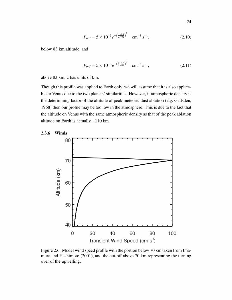
24

Pmd = 5 × 10−3e−(z−832.402

)2

cm−3 s−1, (2.10)

below 83 km altitude, and

Pmd = 5 × 10−3e−(z−838.407

)2

cm−3 s−1, (2.11)

above 83 km. z has units of km.

Though this profile was applied to Earth only, we will assume that it is also applica-ble to Venus due to the two planets’ similarities. However, if atmospheric density isthe determining factor of the altitude of peak meteoric dust ablation (e.g. Gadsden,1968) then our profile may be too low in the atmosphere. This is due to the fact thatthe altitude on Venus with the same atmospheric density as that of the peak ablationaltitude on Earth is actually ∼110 km.

2.3.6 Winds

Figure 2.6: Model wind speed profile with the portion below 70 km taken from Ima-mura and Hashimoto (2001), and the cut-off above 70 km representing the turningover of the upwelling.

25

In addition to testing the effects of the nucleation of sulfuric acid droplets on mete-oric dust on the UH particle size distribution, we will also test the effects of transientgusts at the cloud tops. These are a separate set of simulations from the nominalruns described in §2.3.1, though they do use the results of the nominal runs as initialconditions. Figure 2.6 shows the wind profile we use to test the effects of transientupward winds on the number density and size distribution of the cloud and hazeaerosols. The wind beneath 70 km is a constant flux wind similar to that of Ima-mura and Hashimoto (2001) but increased in strength by two orders of magnitudeto simulate a gust as opposed to a branch of the global circulation:

w =8 × 10−3

ρcm s−1, (2.12)

where w is upward wind speed and ρ is atmospheric density, both in cgs units.In order to adhere to our top boundary condition and simulate turning over of thewind currents, we allow the upward wind to fall off linearly above 70 km so thatit vanishes at 75 km. This is consistent with the strong static stability above thataltitude.

Recent Venus Express observations of the Venus southern polar vortex at the al-titude of the upper cloud (63–69 km) show divergent and convergent circulationsthat imply vertical velocities of ∼0.2 m s−1 (Garate-Lopez et al., 2013), roughlyconsistent with the lower limits of our upper cloud wind velocities, though most ofthe vertical motions were downward rather than upward. In addition, convectivecells at the cloud tops have been observed at and downwind of the Venus subsolarpoint (Belton et al., 1976; Titov et al., 2012). These have been interpreted using2D convection simulations as the incursion of the convective region in the mid-dle cloud into the stably stratified upper cloud (Baker, Schubert, and Jones, 1998;Baker, Schubert, and Jones, 1999), though some recent observations suggest thatthe convective layer is thin enough that it may only occupy the upper cloud itself(Markiewicz et al., 2007). The results of Baker, Schubert, and Jones (1998) suggestthat gravity waves originating from the enlarged convective region could producevertical velocities of 1–2 m s−1 at and above 60 km, matching our wind velocitiesat those altitudes.

Nevertheless, there are clear differences between our vertical advection scheme andthe actual advection processes in the Venus clouds. For instance, a realistic treat-ment of the gust “turning over” above 70 km requires horizontal transport, which

26

is beyond the scope of this study. Thus, for the purpose of this work we will onlyexamine qualitatively the effects of such a gust on the cloud profile, such as theformation of a detached haze due to upwelled cloud particles, its destruction due tosedimentation and diffusion, the time scales involved, and the changes in particlesize distributions. In order to better evaluate these effects, we will magnify themby considering gusts that last for 5 × 104 seconds, or ∼14 Earth hours. Gusts in thepolar vortex may last as long, though as Venus Express orbits Venus on the sametime scale (∼1 Earth day), the actual duration is uncertain. Winds caused by subso-lar point convection may also be able to last 14 hours, as convective features wereseen up to 50 latitude away from the equator (Titov et al., 2012). This should alsoapply to longitude, and a distance of 50 longitude away from the subsolar pointcan be covered by the ∼100 m s−1 planet-encircling zonal winds at the cloud tops(Schubert et al., 1980) in about 14 hours. In other words, each parcel of air couldhave 14 hours during which gusts arising from subsolar convection can disrupt theaerosol particle distributions therein before the convective cells give way to stablystratified regions. Nevertheless, not only is the wind unlikely to be constant giventhe turbulent nature of its origin, but Wilquet, Fedorova, et al. (2009) observed thehaze at ∼ 50, a full 20 latitude away from the convective region. In short, weare not looking for exact agreement between our particle number density and sizedistributions and one that is retrieved from observations, but rather whether we canqualitatively reproduce the chaotic behavior of the UH.

2.4 Results & DiscussionOur steady state results do not show a stable equilibrium distribution, but rather aquasi-periodically varying distribution. Thus, we will proceed to compare to ob-servations our results from a single time step near the end of our nominal modelrun that best match them (§2.4.1), and then describe the mechanisms that couldallow for such dynamics to occur despite a constant background atmospheric state(§2.4.2). In §2.4.3 we discuss the effect of decreasing the sulfur production rate,and in §2.4.4 we will describe our transient wind results.

2.4.1 Nominal ResultsFigure 2.7 shows the number density predictions from our model for particles withradii greater than ∼0.1 µm, which we choose as the lower size boundary of mode1/small mode particles (Wilquet, Fedorova, et al., 2009). We see that it is largelyconsistent with LCPS cloud data (Knollenberg and Hunten, 1980), though the mid-

27

Figure 2.7: Number density of cloud and haze particles with radius r > 0.115 µm(solid line) from the nominal model compared to total number density data fromLCPS (filled circles) (Knollenberg and Hunten 1980) and Venus Express (pluses)(Wilquet, Fedorova, et al. 2009).

dle cloud is overestimated by a factor of 3 and the lower cloud is underestimatedby a factor of <2. These differences are well within the range of variability seenat these levels by the Pioneer Venus entry probes (Esposito et al., 1983), or in nearinfrared observations of the Venus night side (Crisp, Ingersoll, et al., 1990; Grin-spoon et al., 1993). Figure 2.8 shows the size distributions of the cloud and hazeparticles at various altitudes. It reproduces both the high number density of mode1 particles in the upper cloud and the distinct multi-modal nature of the middle andlower clouds’ particle size distributions as seen by Pioneer Venus (Knollenberg andHunten, 1980), including mode 1 at ∼0.2 µm, mode 2 at ∼1.4 µm, and mode 3 (nearthe cloud base) at ∼3.5 µm. Comparison of this size distribution with Pioneer Venusobservations at 54.2 km (Knollenberg and Hunten, 1980) shows clear agreement be-tween the model mode radii and that of the data, though a discrepancy exists in themode abundances, as there is an order of magnitude less mode 3 particles and ∼3times more mode 2 particles in our model than in the observations. These discrep-ancies could be caused by the lack of transient gusts in the middle and lower clouds

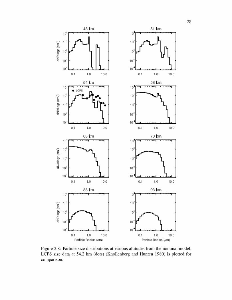
28

Figure 2.8: Particle size distributions at various altitudes from the nominal model.LCPS size data at 54.2 km (dots) (Knollenberg and Hunten 1980) is plotted forcomparison.

29

of our steady state model, which Imamura and Hashimoto (2001) showed could beused to produce a multi-modal structure in their model. Physically, vertical gustssuch as those detected in the middle cloud by the VEGA balloons (Crisp, Ingersoll,et al., 1990) would both aid in the growth of mode 2 particles into mode 3 particlesby introducing “fresh” sulfuric acid from below (updrafts) and in the depletion ofthe middle cloud by downwelling the cloud particles (downdrafts); the depletion ofthe middle cloud is also a natural consequence of the growth of particles, as theselarger particles would have a faster sedimentation time. Therefore, a series of ver-tical updrafts and downdrafts could lead to fewer mode 2 particles, more mode 3particles, and fewer particles in the middle cloud, resulting in better agreement withdata.

We assume that mode 3 particles are just larger versions of mode 2 particles, i.e.they are liquid sulfuric acid droplets with a solid polysulfur component, but thisneed not be the case. In fact, (Knollenberg and Hunten, 1980) discussed the pos-sibility that mode 3 is made up of solid, crystalline particles. On the other hand,Toon, Ragent, et al. (1984) suggested that mode 3 is in fact a large particle tail ofmode 2; our results support this latter interpretation, as the mode 3 particle peakblends into the mode 2 peak somewhere between 54 and 58 km (Figure 2.8). Inlight of the results of Young (1983), however, we must consider the effect of solidpolysulfur “patches” on the surface of our sulfuric acid particles, which may makethem seem like solid, crystalline particles if the polysulfur coverage is high enough.As previously stated, the effect of these patches is the decrease in the efficiency ofcoagulation in the removal of smaller particles, creating a smaller number of largerparticles. This could explain our underestimation of the lower cloud particle numberdensity, though it would also further overestimate our middle cloud particle numberdensity. Thus, a combination of decreased coagulation efficiency in larger particlesand the addition of middle cloud vertical gusts may be necessary to improve ourmodel’s agreement with the Pioneer Venus Sounder Probe observations.

In the UH, our model predicts a steady state size distribution that is roughly mono-modal, with a small “bump” at radii > 1 µm corresponding to upwelled mode 2particles that is largely insignificant compared to the rest of the distribution. Thelack of distinct bimodality despite the two different sources of particles is likelydue to the effects of coagulation. In Figure 2.9, we follow the time evolution ofthe upper haze at an altitude of 84 km during the first ∼4 months of the modelrun, long before steady state is reached. The green “bar” at 0.01 µm is caused by

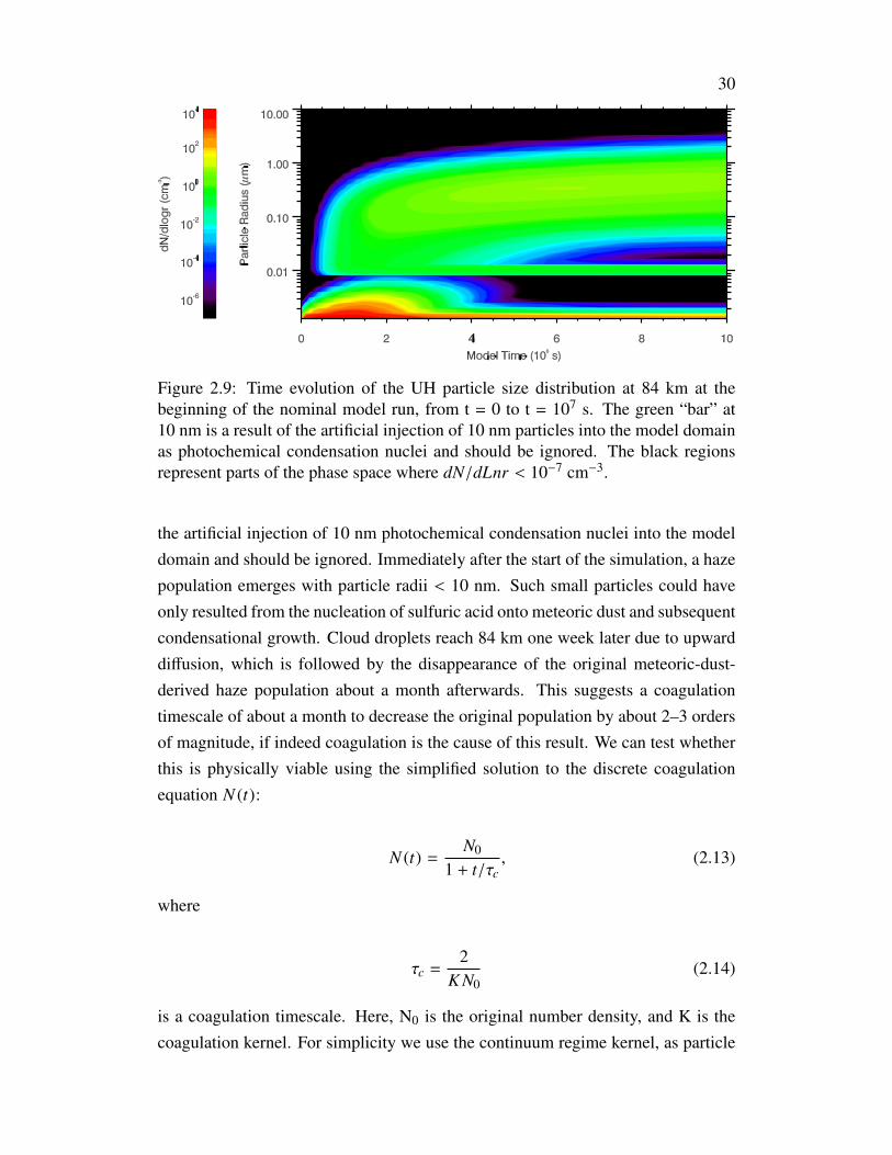
30

Figure 2.9: Time evolution of the UH particle size distribution at 84 km at thebeginning of the nominal model run, from t = 0 to t = 107 s. The green “bar” at10 nm is a result of the artificial injection of 10 nm particles into the model domainas photochemical condensation nuclei and should be ignored. The black regionsrepresent parts of the phase space where dN/dLnr < 10−7 cm−3.

the artificial injection of 10 nm photochemical condensation nuclei into the modeldomain and should be ignored. Immediately after the start of the simulation, a hazepopulation emerges with particle radii < 10 nm. Such small particles could haveonly resulted from the nucleation of sulfuric acid onto meteoric dust and subsequentcondensational growth. Cloud droplets reach 84 km one week later due to upwarddiffusion, which is followed by the disappearance of the original meteoric-dust-derived haze population about a month afterwards. This suggests a coagulationtimescale of about a month to decrease the original population by about 2–3 ordersof magnitude, if indeed coagulation is the cause of this result. We can test whetherthis is physically viable using the simplified solution to the discrete coagulationequation N (t):

N (t) =N0

1 + t/τc, (2.13)

where

τc =2

K N0(2.14)

is a coagulation timescale. Here, N0 is the original number density, and K is thecoagulation kernel. For simplicity we use the continuum regime kernel, as particle

31

number density is small, and assume that the particle radii R2 R1:

K ∼2kT3µ

R2

R1(2.15)

(Seinfeld and Pandis, 2006). For a Boltzmann’s constant k = 1.38 × 10−16 erg K−1,temperature T ∼ 160 K, atmospheric viscosity µ ∼ 8× 10−5 g cm−1 s−1 and particleradii R1 = 1 nm and R2 = 100 nm, we get a coagulation time needed to reduce thenumber density by ∼2–3 orders of magnitude of a few months, similar to our modelresults. Therefore we can conclude that the UH is likely a combination of upwelledcloud particles and particles nucleated in situ on meteoric dust, but that the latterpopulation has “fused” with the former, resulting in a mono-modal size distributionin steady state. Thus, two separate sources of particles—one upwelled from below,and one nucleated in situ cannot explain the bimodality detected by Kawabata et al.(1980) and Wilquet, Fedorova, et al. (2009). However, our peak model cloud tophaze particle radius, ∼0.3 µm at 70 km, is fairly close to the average haze particleradius originally detected by Kawabata et al. (1980) (0.23 ± 0.04 µm). Furthermore,our UH size distribution covers the size range of both the small and the large modedetected by Wilquet, Fedorova, et al. (2009). Therefore, we propose that our resultsrepresent both modes, and that something else is responsible for the splitting ofthe particle population into two distinct modes. Figure 2.7 shows a comparisonbetween the model number density and the sum of the number densities of the twomodes detected by Wilquet, Fedorova, et al. (2009). The agreement between modeland data is satisfactory up to 80 km, above which the model underestimates thenumber density by about half an order of magnitude.

Alternatively, the meteoric dust production profile could be at a much higher alti-tude (see §2.3.5) such that they are above the upwelled cloud particles; the sulfuricacid droplets that nucleate onto these meteoric dust particles would then have timeto grow before they sediment into the altitudes dominated by cloud droplets, withwhich they will coagulate as before. In this scenario, the small mode would consistof both the upwelled cloud particles and the sedimenting particles that nucleated insitu onto meteoric dust, while the larger mode would be made up of the productsof small mode coagulation. However, the resulting smaller R2/R1 ratio (Eq. 2.15)would increase the coagulation time scale and decrease the amount of large modeparticles that can be produced. Ultimately, the particles that nucleate from meteoricdust may be inconsequential due to the lower flux of meteoric dust as compared tothe flux of sulfuric acid vapor and sulfur.

32

Figure 2.10: Sulfuric acid vapor mixing ratio from the nominal model (short lines)compared with the sulfuric acid saturation vapor pressure over a flat surface (solid)(§2.3.2) and Magellan radio occultation data analyzed by Kolodner and Steffes(1998) (filled circles).

Figure 2.10 shows a comparison between the predicted mixing ratio of sulfuricacid vapor and the observed mixing ratio from Magellan radio occultation dataas analyzed by Kolodner and Steffes (1998). Though the large dispersion in thedata from 0–6 ppm allows for a wide variety of results to “fit” it, the physicallyrelevant results are likely those that exhibit a local sulfuric acid maximum below theclouds, and which also fit the nonzero data points. Indeed, our model results showa satisfactory fit to the data points. While the bottom boundary condition fixes thevapor concentration to 3 ppm at 40 km, the vapor concentration peak of ∼4.5 ppmat the cloud base is entirely due to sedimenting particles evaporating and depositingtheir sulfuric acid vapor at that altitude. The peak value reflects a balance betweenthe rate of vapor deposition and the upward and downward vapor diffusion, and alsoimposes a constraint on the altitude of the cloud base, below which any sulfuricacid droplets will be evaporating. Our results show that the cloud base is at ∼47km, consistent with the model results of Krasnopolsky and Pollack (1994). Abovethe cloud base, the vapor profile largely follows the saturation vapor pressure curve

33

except at (1) 61 km, where sulfuric acid vapor is photochemically produced, and (2)above 80 km. This latter deviation may be caused by numerical instabilities causedby the low saturation vapor pressure (∼10−31 mbars) or the phase properties ofsulfuric acid and water solutions in this region (McGouldrick, Toon, and Grinspoon,2011).

Figure 2.11: The nominal particle number density as a function of particle size andaltitude. The black regions represent parts of the phase space where dN/dlogr <10−7 cm−3.

Figure 2.11 shows number density as a function of both altitude and particle radius,while Figure 2.12 shows the sulfuric acid and particle mass fluxes for the middlecloud (top) and the other altitudes (bottom); together they give a summary of theprocesses occurring in the clouds and UH of Venus. The production of involatile

34

Figure 2.12: The nominal sulfuric acid vapor (dashes) and particle (short lines)mass fluxes at steady state at the same time step as in figures 7, 8, 10, and 11expressed in units of mass equivalent to 1012 sulfuric acid molecules per unit areaper second, where each molecule has mass MSA ∼ 1.6 × 10−22 g. Note the differentaxes scales between the top and bottom panels: the top panel shows the high fluxvalues of the middle cloud, while the bottom panel shows the lower flux values atthe other altitudes.

sulfur condensation nuclei causes the nucleation and condensational growth of liq-uid sulfuric acid droplets at 61 km, resulting in a high number density of mode 1particles. These particles then diffuse upwards and sediment downwards. The posi-tive divergence in the particle flux (in units of mass equivalent to 1012 sulfuric acidmolecules per unit area per second, where each molecule has mass ∼ 1.6× 10−22 g)

35

in this region is clearly shown by the positive slope at ∼61 km in the lower panel ofFigure 2.12—particles higher up has a smaller downward flux (i.e. a less negativeflux) than the particles lower down. There is no corresponding slope in the vaporflux curve as all the vapor is condensing onto the particles. In the UH, the upwarddiffusion of particles appears to balance the sedimentation, leading to a near zeroparticle flux; the sulfuric acid vapor flux is also very close to zero, but it is likelydue to the small amount of vapor at these altitudes.

Below 61 km, the vigorous convection in the middle cloud drives the large upwardflux of sulfuric acid vapor (top panel of Figure 2.12), resulting in enhanced pro-duction of mode 2 particles as well as a tail of even larger particles resulting fromcoagulation. These particles, like the upper cloud particles, are transported down-wards by sedimentation and upwards by diffusion. The latter process leads to asmall large particle bump in the UH. These particles evaporate upon reaching thecloud base, leading to the regeneration of mode 1 particles and the deposition of sul-furic acid vapor beneath the clouds. The regenerated mode 1 is larger than the mode1 of the upper cloud due to the coagulation of the droplets higher up in the clouds—the cores of these droplets are in effect added together, leading to the generation oflarger involatile particles as the larger cores are exposed upon droplet evaporation.This may not be what actually happens if the “cores” are instead patches of poly-sulfur decorating the outside of the sulfuric acid droplets, as per the “gumdrop”model of Young (1983). In this case, the “cores” would not be added together andwould remain the same size as their upper cloud counterparts upon the evaporationof the sulfuric acid. Meanwhile, the tail of large particles forms a distinct thirdmode upon evaporation due to its slower evaporation rate as compared to that of thesmaller mode 2 particles, which is a product of the Kelvin effect (Eq. 2.4).

Below the clouds, the sulfuric acid vapor exhibits a negative flux as discussed pre-viously, while the particle flux is similarly negative, as the particles are sedimentingout of the bottom of the model domain. The absolute value of the sum of the twofluxes at the bottom of the model domain is ∼ 9 × 1011 cm−2 s−1, slightly higherthan the sum of the input flux of meteoric dust (∼ 5×105 cm−2 s−1), photochemicalcondensation nuclei (∼ 1011 cm−2 s−1), and sulfuric acid vapor (6 ∼ 1011 cm−2

s−1). This is due to the quasi-periodically varying nature of our results, i.e. we haveexamined our simulated Venus cloud-haze system at a time when the flux out of thelower model boundary is higher than what it should be for a steady state (∼ 6.83511

cm−2 s−1).

36

2.4.2 Periodic Behavior and Precipitation on Venus

Figure 2.13: Time evolution of the nominal particle size distribution at 84, 74, 64,and 54 km from t = 108 s to t = 2×108 s. Note the different number density contourand y axis scale for the 84 km plot. The black regions represent parts of the phasespace where dN/dlogr < 10−7 cm−3 at 74, 64, and 54 km, and < 0.1 cm−3 at 84km.

Figure 2.13 shows the time evolution of the particle size distribution at variousaltitudes. Above the clouds, the quasi-periodic variations are very small, with am-plitudes of no more than 10%. In the upper cloud, the variations are larger withsmall hints of quasi-periodicity in the mode 2 particle abundances apparent, but thesize distribution is dominated by mode 1 particles, which are fairly stable. In con-

37

trast, the middle cloud shows variations in particle abundances of several orders ofmagnitude. All three modes appear to grow in radii with time and are subsequentlyreplaced with smaller particles on a time scale of ∼6 Earth months. In particular,mode 1 slowly grows to larger radii via coagulation and condensation until reaching∼0.25 µm, where there is a rapid growth of particles to mode 2. This actually occursat several points during the slow migration of mode 1 particles to larger radii, as theintense eddy diffusion at 54 km will allow any particles large enough to overcomethe Kelvin barrier to grow rapidly. The upward diffusion of mode 1 particles frombelow then “resets” the mean mode 1 particle radius back to ∼0.2 µm. Mode 2 thenalso grow slowly with time before growing somewhat rapidly into mode 3 parti-cles, which then proceed to sediment into lower altitudes. The increase in mode 2particle growth rate occurs at nearly the same time as the rapid growth of mode 1particles into mode 2 particles, possibly due to the coagulation of the “new” mode2 particles among themselves and with the “old” mode 2 particles, leading to thecreation of the larger mode 3 particles.

Figure 2.13 also shows that, in comparison with the nominal/best-fit results in§2.4.1, the “usual state” of the Venus clouds is actually not those observed by theLCPS—for the majority of the time, mode 2 has a mean radius of ∼1.2 µm insteadof the observed 1.4 µm (Knollenberg and Hunten, 1980), and it only grows to sucha size right before the emergence of a “new” mode 2.

This oscillation is apparently perpetuated by the growth of mode 1 particles intosizes capable of overcoming the Kelvin Barrier, as that leads to the perturbation ofthe established mode 2 particles which in turn leads to their growth into mode 3particles. The growth of mode 1 particles can occur via coagulation among them-selves, though it is more likely that the majority of coagulation events are with thelarge number of smaller particles we use in our model as photochemical conden-sation nuclei and which grew from those nuclei but have not yet reached the sizesof the mode 1 particles, as coagulation between particles of vastly difference sizesis faster than coagulation between similarly sized particles (Seinfeld and Pandis,2006). As such, since each coagulation event would only add a very small amountof mass to each mode 1 particle, the growth would be gradual but steady, matchingwhat we see in our model results. It is interesting to note that this does not happenwhen we use a larger particle as our photochemical condensation nuclei (e.g. Ima-mura and Hashimoto, 2001), as coagulation would be much slower and “random”in time. These variations also do not happen to such an extent in the UH, as both

38

the coagulation kernel (Eq. 2.15) and condensational growth rate are much lowerthere.

Figure 2.14: The time evolution of the nominal sulfuric acid vapor (dashes) andparticle (short lines) mass fluxes at the bottom of the model domain from t = 108

s to t = 2 × 108 s plotted with the average of the total flux during this time period(solid), all expressed in units of mass equivalent to 1012 sulfuric acid molecules perunit area per second, where each molecule has mass MSA ∼ 1.6 × 10−22 g. Thenegative values indicate downward fluxes.

The quasi-periodic variability of the middle cloud leads to a quasi-periodic sed-imentation flux for the largest particles, which leads to the larger-than-expectedbottom boundary flux in Figure 2.12. Figure 2.14 shows the time evolution of thesulfuric acid vapor and particle flux out of the bottom boundary of the model do-main, expressed in the same units as Figure 2.12. The average of these oscillations,6.765 × 1011 cm−2 s−1 matches the injection rate of mass into the model domain,6.835 × 1011 cm−2 s−1 fairly well, indicating that we are indeed at an equilibriumstate. Finally, we note that the particle and vapor flux oscillations are in phase witheach other, and that the latter has greater amplitude than the former. This is ex-plained by the evaporation of the particles below the cloud deck at ∼47 km, suchthat the sulfuric acid variations from the middle cloud are mostly expressed in theresulting vapor.

39

The possibility of such long term, quasi-periodic particle size variations providetantalizing hints towards possible sulfuric acid “rain” below the cloud decks ofVenus, though we use the term loosely as the downward mass fluxes associatedwith the “rain” in our model results are far smaller than that of typical rain eventson Earth. Nonetheless, it would be interesting to search for evidence of their exis-tence in VIRTIS observations of the Venus night side, which are sensitive to suchvariations in particle population.

2.4.3 Variations in the Sulfur Production RateAs discussed in §2.3.1, the production rate of sulfur in the Venus atmosphere maybe much lower than half the production rate of sulfuric acid as implied by [R2.1]due to reactions of S with O2 and the formation of S2O instead of SO2 and S fromthe reaction SO + SO. To address the effect decreasing the sulfur production wouldhave on our results we rerun our model with both one order of magnitude less sulfurproduced and two orders of magnitude less sulfur produced. Figure 2.15 shows ourresults in terms of the number density (top) and size distribution at 54 km in themiddle cloud (bottom). Decreasing the sulfur condensation nuclei production ratedecreases the number of cloud droplets produced at all altitudes, but also increasesthe average size of the droplets, since there are fewer nuclei for the same amount ofgas to condense on. Mode 1 particle abundances also decrease significantly in themiddle cloud when sulfur production is reduced, as the relative fraction of mode 1particles that grow to mode 2 particles is now much larger. The disagreement be-tween the observed size distribution and the results of the reduced sulfur cases sug-gest that either (1) the primary reaction in the production of sulfur is indeed [R2.1](§2.3.1), and that O2 is relatively scarce in the upper cloud, or (2) Pioneer Venustook data during a period of time when SO2 abundance exceeded O2 abundance,perhaps due to an updraft (Toon, Turco, and Pollack, 1982), and that the “steadystate” size distribution in the middle cloud is more akin to the reduced sulfur cases,with a low mode 1 abundance, or (3) our model is missing several pieces of essen-tial physics, such as the microphysics of the sulfur particles, which would otherwiseresult in greater mode 1 abundance even when sulfur production is reduced. Op-tion (3) is unfortunate but likely, given recent modeling results by Carlson (2010),which showed that the ratio between total sulfur mass and total sulfuric acid massin the cloud droplets is on the order of 0.1–1%. We can calculate the same ratio forour model by adding up the masses of the bare condensation nuclei and the sulfurcores of the sulfuric acid droplets and dividing it by the mass of the sulfuric acid in

40

Figure 2.15: The number density (top) and size distribution at 54 km (bottom) ofthe nominal (black), one order of magnitude reduction in sulfur production (or-ange), and two orders of magnitude reduction in sulfur production (green) cases.The curves in the top figure are compared to total number density data from LCPS(filled circles) (Knollenberg and Hunten 1980) and Venus Express (pluses) (Wil-quet, Fedorova, et al. 2009). The histograms in the bottom figure are compared toLCPS size data at 54.2 km (filled circles) (Knollenberg and Hunten 1980).

the droplets. Figure 2.16 shows this ratio for our three sulfur production rate cases.The sulfur-to-sulfuric-acid mass ratio steadily decreases with altitude until the mid-dle cloud, where it quickly decreases due to the turbulence in the region causingincreased condensation of sulfuric acid onto the droplets; the ratio increases belowthe middle cloud as sulfuric acid begins evaporating from the droplets. The best

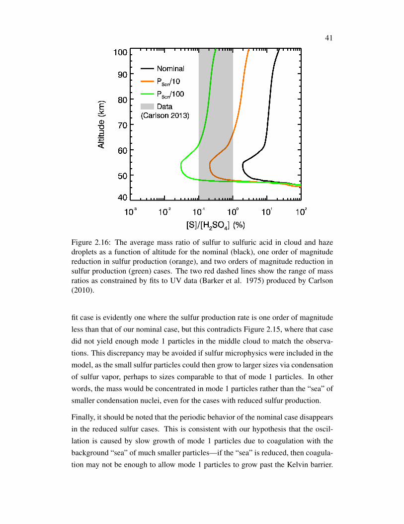
41

Figure 2.16: The average mass ratio of sulfur to sulfuric acid in cloud and hazedroplets as a function of altitude for the nominal (black), one order of magnitudereduction in sulfur production (orange), and two orders of magnitude reduction insulfur production (green) cases. The two red dashed lines show the range of massratios as constrained by fits to UV data (Barker et al. 1975) produced by Carlson(2010).

fit case is evidently one where the sulfur production rate is one order of magnitudeless than that of our nominal case, but this contradicts Figure 2.15, where that casedid not yield enough mode 1 particles in the middle cloud to match the observa-tions. This discrepancy may be avoided if sulfur microphysics were included in themodel, as the small sulfur particles could then grow to larger sizes via condensationof sulfur vapor, perhaps to sizes comparable to that of mode 1 particles. In otherwords, the mass would be concentrated in mode 1 particles rather than the “sea” ofsmaller condensation nuclei, even for the cases with reduced sulfur production.

Finally, it should be noted that the periodic behavior of the nominal case disappearsin the reduced sulfur cases. This is consistent with our hypothesis that the oscil-lation is caused by slow growth of mode 1 particles due to coagulation with thebackground “sea” of much smaller particles—if the “sea” is reduced, then coagula-tion may not be enough to allow mode 1 particles to grow past the Kelvin barrier.

42

This further suggests that the reduced sulfur cases match the true state of the Venusclouds more closely than the nominal case, as no periodic behavior similar to thosein the nominal case has yet been observed.

2.4.4 Transient Wind Results

Figure 2.17: Number density profiles of the upper cloud and haze before (black),immediately after (blue), and 5 × 105 s after (red) a 5 × 104 s transient wind event.The total number density data from LCPS (filled circles) (Knollenberg and Huntenet al. 1980) and Venus Express (pluses) (Wilquet, Fedorova, et al. 2009) are plottedfor comparison. The wind speed profile is shown in Figure 6.

Figure 2.17 gives the number density results before (black), immediately after (blue),and about an Earth week after a transient updraft event lasting ∼14 Earth hours(5 × 104 s) (red), using the wind speed profile given in Figure 2.6. We see that adetached haze layer forms at 75 km with a peak number density 2 orders of mag-nitude greater than the number density at that altitude before the wind event. Thealtitude of the detached haze is likely artificial given our wind profile and the actualmaximum detached haze number density is likely overestimated due to the lack ofhorizontal diffusion aiding (the already present) vertical diffusion in smoothing outthe number density profile. However, the occurrence of an increase in number den-sity at the altitude of the turn-over should be profile-independent. In the week that

43

follows, the detached haze layer diffuses away so that the peak number density ismore than an order of magnitude lower than its maximum immediately followingthe wind event. This shows that such a wind event produces the right time scales forthe observed haze variability from Wilquet, Drummond, et al. (2012), on the orderof days. Furthermore, the diffusion of the detached haze particles upwards resultsin an increase in the number density of the UH such that there is now a much betteragreement between the Wilquet, Fedorova, et al. (2009) UH number density obser-vations and that of our model above 80 km. It is clear, however, that the agreementbetween data and model would be even better if the relaxed distribution was shiftedup by 10 km. This suggests that the turnover was actually 10 km higher in theactual observations, though it is unlikely that such large gusts existed at such highaltitudes.

Figure 2.18: Particle size distribution before (black), immediately after (blue), and5 × 105 s after (red) a 5 × 104 s transient wind event, plotted for various altitudesclose to the turnover altitude of the transient wind. The wind speed profile is shownin Figure 6.

44

Figure 2.18 shows the size distributions at altitudes close to the detached haze layerat the same times as Figure 2.17. Multiple size modes form below the turnover ofthe wind immediately following the wind event (blue). The small mode at ∼0.2µm is largely unchanged from the equilibrium distribution for altitudes below thedetached haze, but is much more abundant within the detached haze itself at 75km; this is caused by the advection of these small particles up to the altitude ofthe detached haze. The “bump” associated with the high altitude tail of the mode2 cloud particles in the equilibrium distribution (black) becomes much more dis-tinct due to upward advection of more mode 2 particles; this feature is much moreprominent below the detached haze, which matches the observations of Wilquet,Fedorova, et al. (2009) where the large UH particle mode (mode 2 cloud particles)number density drops off with altitude much faster than the small UH particle mode(mode 1 cloud particles). The small mode radii covers sizes < 0.6 µm, which is alarger range than the Wilquet, Fedorova, et al. (2009) result of 0.1–0.3 µm; the largemode radii covers the sizes between 0.6 and 1 µm, similar to their results. Beyond1 µm, the particle abundance drops by over an order of magnitude, though a thirdmode does appear resulting from advected mode 3 cloud particles; however, it isinsignificant compared to the small and large modes. Above the turnover, the sizedistribution remains largely mono-modal.

Below the detached haze, the large mode becomes less distinct following the relax-ation period (red), though both modes increase in number density. This is due tothe sedimentation of large mode particles from the detached haze, as we see a largedecrease in number density at the altitude of the detached haze itself. There is alsoan increase in number density above the turnover, as the detached haze particles dif-fuse upwards from the number density maximum. Thus, if the bimodality observedby Wilquet, Fedorova, et al. (2009) was caused by winds, then it was likely transientin nature. This is supported by the order of magnitude variability between extinc-tion profiles of the UH taken only days apart presented in Wilquet, Drummond,et al. (2012). It is unlikely that condensational and coagulational growth play anyimportant role here, as their timescales are far greater than the observed variabilitytimescale (James, Toon, and Schubert, 1997; Seinfeld and Pandis, 2006).

In §2.3.6 we noted the unrealistic long gust duration we have used (∼14 Earthhours). However, we see that the UH size distribution is still visibly disturbedalmost a full Earth week after the wind event in question. If we suppose that ourwind event is caused by subsolar convection near 50 N that lasted for a full 14

45

hours and that the wind was constantly upwards with velocity ∼1 m s−1 at the cloudtop, then given poleward meridional velocities of ∼5 m s−1 (Rossow, Del Benio,and Eichler, 1990) (a high estimate), it would take ∼1 Earth week for this parcel ofair to reach 70 N, the latitude where the measurements of Wilquet, Fedorova, et al.(2009) were taken. It may not be surprising then that our “relaxed” UH numberdensity profile matches the Wilquet, Fedorova, et al. (2009) number density dataso well. However, most of these assumptions are highly optimistic and it is muchmore likely that our results show an exaggeration of what transient winds at thecloud tops can really do to the steady state aerosol distribution.

2.5 Summary & ConclusionsIn this study we simulated the clouds and upper haze of Venus using version 3.0of the microphysical and vertical transport model CARMA. We showed that ap-propriate choices of initial, boundary, and model atmospheric conditions can notonly satisfactorily reproduce the number density and size distributions of the Venusclouds as seen in Pioneer Venus data (Knollenberg and Hunten, 1980), including thebimodal and possible trimodal particle size spectrum and the three separate cloudlayers, but also generate a quasi-periodically varying system rather than a systemwith a stable equilibrium distribution. The disagreements between our results andthe observations—the overestimation of the particle number density and abundanceof mode 2 particles in the middle cloud and the underestimation of the lower cloudand the abundance of mode 3 particles—are all within the range of variability seenin other observations, though the addition of transient gusts in the middle cloud,which would both deplete the middle cloud of particles and create a greater numberof larger particles, may improve our agreement with the Pioneer Venus SounderProbe data.

We also simulated the upper haze as a mixture of droplets formed from in situnucleation of sulfuric acid vapor on meteoric dust and droplets upwelled from thecloud decks below. We showed that the former population rapidly coagulates withthe latter population, resulting in a mono-modal size distribution. Meanwhile, foraltitudes below 80 km there is good agreement between our model particle numberdensities and the sum of the small mode (mode 1) and large mode (mode 2) numberdensities from Wilquet, Fedorova, et al. (2009); above 80 km, we underestimatethe number density by about half an order of magnitude. These particles are likelythose originally observed by the Pioneer Venus OCPP (Kawabata et al., 1980), andcould represent the haze under stable atmospheric conditions. These discrepancies

46

were reduced upon the application of a transient updraft, which created a detachedhaze layer at the altitude of turnover. The diffusion of the detached haze upwardsincreased the particle number density of the UH such that the results agreed with theUH number densities derived by Wilquet, Fedorova, et al. (2009) above 80 km. Theresulting size distribution showed a clear bimodal structure below the detached hazeimmediately after the wind event, with the small mode (mode 1) particles havingradii < 0.6 µm, and the large mode having radii between 0.6 and 1 µm, similar tothe results of Wilquet, Fedorova, et al. (2009). The relaxation of the multi-modalstructures in the size distribution back to a mono-modal distribution had a timescaleof roughly an Earth week, similar to the time scales of haze variability observedby Venus Express (Luz et al., 2011; Markiewicz et al., 2007). The duration andstrength of the updraft were likely exaggerations of what actually takes place in theVenus atmosphere, though subsolar convection could be a viable candidate for thegeneration of these events under optimistic assumptions.

We noted a quasi-periodic variability in our results with a rough period of ∼6 Earthmonths despite a stable background atmospheric state and constant input of sulfuricacid vapor and condensation nuclei. This variability is most apparent in the middlecloud, where steady coagulation of small particles (∼10 nm) with mode 1 particleslead to a slow increase in the mean mode 1 particle radii. Upon reaching the Kelvinbarrier, the mode 1 particles rapidly grow to mode 2 particles via condensationalgrowth, while upward diffusion of mode 1 particles from below replenish the mode1 population. The cycle then repeats and a new wave of mode 2 particles appear;these new mode 2 particles coagulate with the old mode 2 particles, resulting inmode 3 particles that then sediment out of the model domain. This process doesnot occur if the sulfur condensation nuclei production rate is decreased by an or-der of magnitude or more, nor does it occur if the condensation nuclei are larger.Comparison between model results and Pioneer Venus observations (Knollenbergand Hunten, 1980) suggests that the LCPS data may have been taken during one ofthe unstable “growth phases” rather than the much more long-lived stable phases.These episodic variations also leads to periodicity in the magnitude of the sulfuricacid flux out of the bottom boundary of the model domain and suggests possi-ble sulfuric acid “rain events” that could occur immediately below the cloud deck.Such long term variability in particle population should be detectable by VIRTISobservations of the Venus night side.

The sulfur production rate in the upper cloud is uncertain and could be much lower

47

than half of the sulfuric acid production rate as assumed in Imamura and Hashimoto(2001) and in our nominal model. Comparisons with sulfur-to-sulfuric-acid massratios of the cloud droplets derived from UV data (Carlson, 2010) shows that thebest fit case is one where the sulfur production rate is reduced by an order of mag-nitude from that of the nominal case. However, comparison of this case with LCPSparticle size distributions shows that the model predicts mode 1 particle abundancesin the middle cloud two orders of magnitude less what is observed. This discrep-ancy could be caused by the lack of sulfur microphysics in our model, which couldallow the sulfur condensation nuclei to grow to mode 1 particles (∼0.2 µm) insteadof being fixed at a size of ∼10 nm.

It is necessary for future models to include both sulfur and sulfuric acid micro-physics in order to provide a more complete picture of the processes occurringwithin the Venus clouds and hazes. Interactions between aerosols formed fromthese species and their gas phases are diverse and only a subset has been tested.Furthermore, the production rates of these two species, particularly sulfur and itsallotropes, require better constraints from both chemical models that take into ac-count sinks due to aerosol formation and observations that are able to probe downto the altitudes where photochemistry dominates. Finally, continuous observationof the Venus hazes and clouds is essential in constraining their time evolution, es-pecially after transient events.

We thank S. Garimella and R. L. Shia for assistance with the setting up and runningof the CARMA code. We thank R. W. Carlson and C. Parkinson for their valuableinputs. We thank C. Li for his help in speeding up our model runs by more than afactor of 10. This research was supported in part by the Venus Express program viaNASA NNX10AP80G grant to the California Institute of Technology, and in partby an NAI Virtual Planetary Laboratory grant from the University of Washingtonto the Jet Propulsion Laboratory and California Institute of Technology. Part of theresearch described here was carried out at the Jet Propulsion Laboratory, CaliforniaInstitute of Technology, under a contract with the National Aeronautics and SpaceAdministration.

References

Ayers, G. P., R. W. Gillett, and J. L. Gras (1980). “On the vapor pressure of sulfuricacid.” In: Geophysics Research Letters 7, pp. 433–436.

48

Baker, R. D., G. Schubert, and P. W. Jones (1998). “Cloud-level penetrative com-pressible convection in the Venus atmosphere.” In: Journal of the AtmosphericSciences 55, pp. 3–18.

– (1999). “High Rayleigh number compression convection in Venus’ atmosphere:Penetration, entrainment, and turbulence.” In: Journal of Geophysical Research104, pp. 3815–3832.

Bardeen, C. G., A. Conley, et al. (2011). “The CARMA 3.0 microphysics packagein CESM.” Presented at the Whole Atmosphere Working Group Meeting, Boulder,USA.

Bardeen, C. G., O. B. Toon, et al. (2008). “Numerical simulations of the threedimensional distribution of meteoric dust in the mesosphere and upper strato-sphere.” In: Journal of Geophysical Research 113, p. D17202.

Belton, M. J. S. et al. (1976). “Cloud patterns, waves and convection in the Venusatmosphere.” In: Journal of the Atmospheric Sciences 33, pp. 1394–1417.

Bertaux, J-L. et al. (2007). “A warm layer in Venus’ cryosphere and high-altitudemeasurements of HF, HCl, H2O, and HDO.” In: Nature 450, pp. 646–649.

Carlson, R. W. (2010). “Venus’s ultraviolet absorber and sulfuric acid droplets”.Presented at the International Venus Conference, Aussois, France.

Carlson, R. W. et al. (1993). “Variations in Venus cloud properties: A new viewof Venus’s cloud morphology as observed by the Galileo Near-Infrared MappingSpectrometer.” In: Planetary and Space Science 41, pp. 477–485.

Clancy, R. T. and D. O. Muhleman (1991). “Long-term (1979-1990) changes inthe thermal, dynamical, and compositional structure of the Venus mesosphere asinferred from microwave spectral line observations of 12CO, 13CO, and C18O.”In: Icarus 89, pp. 129–146.

Crisp, D., A. P. Ingersoll, et al. (1990). “VEGA Balloon meteorological measure-ments.” In: Advances in Space Research 10, pp. 109–124.

Crisp, D., S. McMuldroch, et al. (1991). “Ground-based near-infrared imaging ob-servations of Venus during the Galileo encounter.” In: Science 253, pp. 1538–1541.

Crisp, D., W. M. Sinton, et al. (1989). “The nature of the near-infrared features onthe Venus night side.” In: Science 246, pp. 506–509.

English, J. M. et al. (2011). “Microphysical simulations of new particle formationin the upper troposphere and lower stratosphere.” In: Atmospheric Chemistry andPhysics 11, pp. 9303–9322.

Esposito, L. W. et al. (1983). “The clouds and hazes of Venus.” In: Venus. Ed. byD. M. Hunten et al. Tucson, USA: University of Arizona Press, pp. 484–564.

Gadsden, M. (1968). “Sodium in the upper atmosphere: Meteoric origin.” In: Jour-nal of Atmospheric and Solar-Terrestrial Physics 30, pp. 151–161.

49

Garate-Lopez, I. et al. (2013). “A chaotic long-lived vortex at the southern pole ofVenus.” In: Nature Geoscience 6, pp. 254–257.

Giauque, W. F. et al. (1959). “The thermodynamic properties of aqueous sulfu-ric acid solutions and hydrates from 15 to 300 K.” In: Journal of the AmericanChemical Society 82, pp. 62–70.

Grinspoon, D. H. et al. (1993). “Probing Venus’s cloud structure with Galileo NIMS.”In: Planetary and Space Science 41, pp. 515–542.

Hueso, R. et al. (2008). “Morphology and dynamics of Venus oxygen airglow fromVenus Express/Visible and Infrared Thermal Imaging Spectrometer observations.”In: Journal of Geophysical Research 113, E00B02.

Hunten, D. M., R. P. Turco, and O. B. Toon (1980). “Smoke and dust particles ofmeteoric origin in the mesosphere and stratosphere.” In: Journal of the Atmo-spheric Sciences 37, pp. 1342–1357.

Ignatiev, N. I. et al. (1997). “Water vapour in the lower atmosphere of Venus: A newanalysis of optical spectra measured by entry probes.” In: Planetary and SpaceScience 45, pp. 427–438.

Imamura, T. (1997). “Momentum balance of the Venusian midlatitude mesosphere.”In: Journal of Geophysical Research 102, pp. 6615–6620.

Imamura, T. and G. L. Hashimoto (2001). “Microphysics of Venusian clouds inrising tropical air.” In: Journal of the Atmospheric Sciences 55, pp. 3597–3612.

Ingersoll, A. P., D. Crisp, and the VEGA Balloon Science Team. (1987). “Estimatesof convective heat fluxes and gravity wave amplitudes in the Venus middle cloudlayer from VEGA balloon measurements.” In: Advances in Space Research 7,pp. 343–349.

Jacobson, M. Z. and R. P. Turco (1994). “Modeling coagulation among particlesof different composition and size.” In: Atmospheric Environment 28, pp. 1327–1338.

James, E. P., O. B. Toon, and G. Schubert (1997). “A numerical microphysicalmodel of the condensational Venus cloud.” In: Icarus 129, pp. 147–171.

Kalashnikova, O. et al. (2000). “Meteoric smoke production in the atmosphere.” In:Geophysical Research Letters 27, pp. 3293–3296.

Kawabata, K. et al. (1980). “Cloud and haze properties from Pioneer Venus po-larimetry.” In: Journal of Geophysical Research 85, pp. 8129–8140.

Knollenberg, R. G. and D. M. Hunten (1980). “The microphysics of the clouds ofVenus: Results of the Pioneer Venus particle size spectrometer experiment.” In:Journal of Geophysical Research 85, pp. 8039–8058.

Kolodner, M. A. and P. G. Steffes (1998). “The microwave absorption and abun-dance of sulfuric acid vapor in the Venus atmosphere based on new laboratorymeasurements.” In: Icarus 132, pp. 151–169.

50

Krasnopolsky, V. A. (1983). “Venus spectroscopy in the 3000–8000 Åregion byVeneras 9 and 10.” In: Venus. Ed. by D. M. Hunten et al. Tucson, USA: Universityof Arizona Press, pp. 459–483.

Krasnopolsky, V. A. and V. A. Parshev (1983). “Photochemistry of the Venus at-mosphere.” In: Venus. Ed. by D. M. Hunten et al. Tucson, USA: University ofArizona Press, pp. 431–458.

Krasnopolsky, V. A. and J. B. Pollack (1994). “H2O - H2SO4 system in Venus’clouds and OCS, CO, and H2SO4 profiles in Venus’ troposphere.” In: Icarus109, pp. 58–78.

Kulmala, M. and A. Laaksonen (1990). “Binary nucleation of water-sulfuric acidsystem: Comparison of classical theories with different H2SO4 saturation vaporpressures.” In: Journal of Chemical Physics 93, pp. 696–701.

Luz, D. et al. (2011). “Venus’s southern polar vortex reveals precessing circulation.”In: Science 332, pp. 577–580.

Lyons, J. R. (2008). “An estimate of the equilibrium speciation of sulfur vapor oversolid sulfur and implications for planetary atmospheres.” In: Journal of SulfurChemistry 29, pp. 269–279.

Markiewicz, W. J. et al. (2007). “Morphology and dynamics of the upper cloudlayer of Venus.” In: Nature 450, pp. 633–636.

McGouldrick, K. and O. B. Toon (2007). “An investigation of possible causes ofthe holes in the condensational Venus cloud using a microphysical cloud modelwith a radiative-dynamical feedback.” In: Icarus 191, pp. 1–24.

McGouldrick, K., O. B. Toon, and D. H. Grinspoon (2011). “Sulfuric acid aerosolsin the atmosphere of the terrestrial planets.” In: Planetary and Space Science 59,pp. 934–941.


Mills, M. J. (1996). “Stratospheric sulfate aerosol: A microphysical model.” PhDthesis. University of Colorado, Department of Astrophysical, Planetary, and At-mospheric sciences.

Rossow, W. B., A. D. Del Benio, and T. Eichler (1990). “Cloud-tracked windsfrom Pioneer Venus OCPP images.” In: Journal of the Atmospheric Sciences 47,pp. 2053–2084.

Sabinina, L. and L. Turpugow (1935). “The surface tension of the system sulfuricacid/water.” In: Zeitschrift für Physikalische Chemie A173, pp. 237–241.

Sandor, B. J., R. T. Clancy, and G. Moriarty-Schieven (2012). “Upper limits forH2SO4 in the mesosphere of Venus.” In: Icarus 217, pp. 839–844.

51

Saunders, R. W. et al. (2012). “Interactions of meteoric smoke particles with sul-phuric acid in the Earth’s stratosphere.” In: Atmospheric Chemistry and Physics12, pp. 4387–4398.

Schubert, G. et al. (1980). “Structure and circulation of the Venus atmosphere.” In:Journal of Geophysical Research 85, pp. 8007–8025.

Seiff, A., D. B. Kirk, et al. (1980). “Measurements of thermal structure and thermalcontrasts in the atmosphere of Venus and related dynamical observations: Resultsfrom the four Pioneer Venus probes.” In: Journal of Geophysical Research 85,pp. 7903–7933.

Seiff, A., J. T. Schofield, et al. (1985). “Models of the structure of the atmosphereof Venus from the surface to 100 kilometers altitude.” In: Advances in SpaceResearch 5, pp. 3–58.

Seinfeld, J. H. and S. N. Pandis (2006). Atmospheric chemistry and physics: Fromair pollution to climate change, 2nd edition. John Wiley & Sons, Inc. Hoboken,New Jersey, USA.

Tabazadeh, A. et al. (1997). “A new parameterization of H2SO4/H2O aerosol com-position: Atmospheric implications.” In: Geophysical Research Letters 24, pp. 1931–1934.

Tellmann, S. et al. (2009). “Structure of the Venus neutral atmosphere as observedby the Radio Science experiment VeRa on Venus Express.” In: Journal of Geo-physical Research 114, E00B36.

Titov, D. V. et al. (2012). “Morphology of the cloud tops as observed by the VenusExpress Monitoring Camera.” In: Icarus 217, pp. 682–701.

Toon, O. B., B. Ragent, et al. (1984). “Large, solid particles in the clouds of Venus:Do they exist?” In: Icarus 57, pp. 143–160.

Toon, O. B., R. P. Turco, J. Jordan, et al. (1989). “Physical processes in polar strato-spheric ice clouds.” In: Journal of Geophysical Research 94, pp. 11359–11380.

Toon, O. B., R. P. Turco, and J. B. Pollack (1982). “The ultraviolet absorber onVenus: Amorphous sulfur.” In: Icarus 51, pp. 358–373.

Toon, O. B., R. P. Turco, D. Westphal, et al. (1988). “A multidimensional model foraerosols: Description of computational analogs.” In: Journal of the AtmosphericSciences 45, pp. 2123–2143.

Turco, R. P., P. Hamill, et al. (1979). “A one-dimensional model describing aerosolformation and evolution in the stratosphere: I. Physical processes and mathemat-ical analogs.” In: Journal of the Atmospheric Sciences 36, pp. 699–717.

Turco, R. P., O. B. Toon, et al. (1983). “Venus: Mesospheric hazes of ice, dust, andacid aerosols.” In: Icarus 53, pp. 18–25.

White, F. M. (1974). Viscous Fluid Flow. McGraw-Hill, New York, USA.

52

Wilquet, V., R. Drummond, et al. (2012). “Optical extinction due to aerosols in theupper haze of Venus: Four years of SOIR/VEX observations from 2006 to 2010.”In: Icarus 317, pp. 875–881.

Wilquet, V., A. Fedorova, et al. (2009). “Preliminary characterization of the upperhaze by SPICAV/SOIR solar occultation in UV to mid-IR onboard Venus Ex-press.” In: Journal of Geophysical Research 114, E00B42.

Yamamoto, M. and M. Takahashi (2006). “An aerosol transport model based ona two-moment microphysical parametrization in the Venus middle atmosphere:Model description and preliminary experiments.” In: Journal of Geophysical Re-search 111, E08002.

Yamamoto, M. and H. Tanaka (1998). “The Venusian Y-shaped cloud pattern basedon an aerosol-transport model.” In: Journal of the Atmospheric Sciences 55,pp. 1400–1426.

Young, A. T. (1983). “Venus cloud microphysics.” In: Icarus 56, pp. 568–577.

Yung, Y. L. and W. B. DeMore (1982). “Photochemistry of the stratosphere ofVenus: Implications for atmospheric evolution.” In: Icarus 51, pp. 199–247.

Zhang, X., M. C. Liang, F. P. Mills, et al. (2012). “Sulfur chemistry in the middleatmosphere of Venus.” In: Icarus 217, pp. 714–739.

Zhang, X., M. C. Liang, F. Montmessin, et al. (2010). “Photolysis of sulphuricacid as the source of sulphur oxides in the mesosphere of Venus.” In: NatureGeoscience 3, pp. 834–837.

Zhang, X., S. N. Pandis, and J. H. Seinfeld (2012). “Diffusion-limited versus quasi-equilibrium aerosol growth.” In: Aerosol Science and Technology 46, pp. 874–885.

53

PART II: FROZEN FRACTALS ALL AROUND

54

C h a p t e r 3

CONSTRAINTS ON THE MICROPHYSICS OF PLUTO’SPHOTOCHEMICAL HAZE FROM NEW HORIZONS

OBSERVATIONS

Gao, P. et al. (Accepted). “Constraints on the Microphysics of Pluto’s Photochem-ical Haze from New Horizons Observations”. In: Icarus. doi: 10 . 1016 / j .icarus.2016.09.030.

3.1 AbstractThe New Horizons flyby of Pluto confirmed the existence of hazes in its atmo-sphere. Observations of a large high to low phase brightness ratio, combined withthe blue color of the haze (indicative of Rayleigh scattering), suggest that the hazeparticles are fractal aggregates, perhaps analogous to the photochemical hazes onTitan. Therefore, studying the Pluto hazes can shed light on the similarities anddifferences between the Pluto and Titan atmospheres. We model the haze distribu-tion using the Community Aerosol and Radiation Model for Atmospheres assum-ing that the distribution is shaped by downward transport and coagulation of par-ticles originating from photochemistry. Hazes composed of both purely sphericaland purely fractal aggregate particles are considered. General agreement betweenmodel results and solar occultation observations is obtained with aggregate particleswhen the downward mass flux of photochemical products is equal to the column-integrated methane destruction rate ∼1.2 × 10−14 g cm−2 s−1, while for sphericalparticles the mass flux must be 2–3 times greater. This flux is nearly identical tothe haze production flux of Titan previously obtained by comparing microphysicalmodel results to Cassini observations. The aggregate particle radius is sensitiveto particle charging effects, and a particle charge to radius ratio of 30 e−/µm isnecessary to produce ∼0.1–0.2 µm aggregates near Pluto’s surface, in accordancewith forward scattering measurements. Such a particle charge to radius ratio is 2–4times higher than those previously obtained for Titan. Hazes composed of sphereswith the same particle charge to radius ratio have particles that are 4 times smallerat Pluto’s surface. These results further suggest that the haze particles are frac-tal aggregates. We also consider the effect of condensation of HCN, C2H2, C2H4,and C2H6 on the haze particles, which may play an important role in shaping their

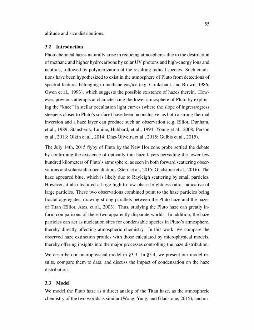
55

altitude and size distributions.

3.2 IntroductionPhotochemical hazes naturally arise in reducing atmospheres due to the destructionof methane and higher hydrocarbons by solar UV photons and high-energy ions andneutrals, followed by polymerization of the resulting radical species. Such condi-tions have been hypothesized to exist in the atmosphere of Pluto from detections ofspectral features belonging to methane gas/ice (e.g. Cruikshank and Brown, 1986;Owen et al., 1993), which suggests the possible existence of hazes therein. How-ever, previous attempts at characterizing the lower atmosphere of Pluto by exploit-ing the “knee” in stellar occultation light curves (where the slope of ingress/egresssteepens closer to Pluto’s surface) have been inconclusive, as both a strong thermalinversion and a haze layer can produce such an observation (e.g. Elliot, Dunham,et al., 1989; Stansberry, Lunine, Hubbard, et al., 1994; Young et al., 2008; Personet al., 2013; Olkin et al., 2014; Dias-Oliveira et al., 2015; Gulbis et al., 2015).

The July 14th, 2015 flyby of Pluto by the New Horizons probe settled the debateby confirming the existence of optically thin haze layers pervading the lower fewhundred kilometers of Pluto’s atmosphere, as seen in both forward scattering obser-vations and solar/stellar occultations (Stern et al., 2015; Gladstone et al., 2016). Thehaze appeared blue, which is likely due to Rayleigh scattering by small particles.However, it also featured a large high to low phase brightness ratio, indicative oflarge particles. These two observations combined point to the haze particles beingfractal aggregates, drawing strong parallels between the Pluto haze and the hazesof Titan (Elliot, Ates, et al., 2003). Thus, studying the Pluto haze can greatly in-form comparisons of these two apparently disparate worlds. In addition, the hazeparticles can act as nucleation sites for condensable species in Pluto’s atmosphere,thereby directly affecting atmospheric chemistry. In this work, we compare theobserved haze extinction profiles with those calculated by microphysical models,thereby offering insights into the major processes controlling the haze distribution.

We describe our microphysical model in §3.3. In §3.4, we present our model re-sults, compare them to data, and discuss the impact of condensation on the hazedistribution.

3.3 ModelWe model the Pluto haze as a direct analog of the Titan haze, as the atmosphericchemistry of the two worlds is similar (Wong, Yung, and Gladstone, 2015), and un-

56

certainties on the processes governing the formation and evolution of Titan’s hazeare much smaller than that of Pluto’s haze owing to 10 years of Cassini observa-tions. Possible differences between the hazes on these two worlds are discussed in§3.4.1.

Titan’s haze is composed of fractal aggregates—fluffy, porous particles consist-ing of smaller subunits, or “monomers” (West and Smith, 1991). The number ofmonomers, Nm, in an aggregate particle is defined as

Nm =

(R f

rm

)D f

, (3.1)

where R f is the effective particle radius of the aggregate, rm is the monomer radius,and D f is the fractal dimension of the aggregate, typically between 1.75 and 2.5for Titan haze particles (Cabane et al., 1993). For simplicity we use D f = 2 in ourmodeling. Eq. 3.1 can be used to find the mass M of an aggregate, which for D f =

2 is

M =43πρprm R2

f , (3.2)

where ρp = 1 g cm−3 is the monomer mass density (Lavvas, Yelle, and Griffith,2010). Gladstone et al. (2016) estimated rm to be ∼10 nm for Pluto’s haze particlesusing Rayleigh scattering, and thus we adopt this value for our nominal model. Wealso consider 5 nm monomers, under the hypothesis that monomers can grow bycondensation of simple hydrocarbons and nitriles (Barth, 2014; Wong, Fan, et al.,2016).

We use the same model atmosphere as for the photochemical calculations of Wong,Fan, et al. (2016), though we focus only on altitudes below 500 km to avoid spend-ing computational time on altitudes where data quality is low. Figure 3.1 showsthe temperature profile of the model atmosphere, updated from Zhu, Strobel, andErwin (2014).

We calculate the equilibrium haze particle size and altitude distribution using the 1–dimensional Community Aerosol and Radiation Model for Atmospheres (CARMA;Turco et al., 1979; Toon, Turco, et al., 1988; Jacobson and Turco, 1994; Bardeen etal., 2008; Wolf and Toon, 2010). CARMA is a Eulerian forward model that solvesthe discretized continuity equation for aerosol particles subject to vertical transport

57

Figure 3.1: (Left) The temperature (black) and net condensation rate profiles forHCN (red), C2H2 (yellow), C2H4 (green), and C2H6 (blue) taken from the photo-chemical model results of Wong, Fan, et al. (2016). (Right) The same as the leftplot but zoomed into the lower 20 km of the atmosphere, where C2H6 condensationdominates over the other species. Note the different bottom x-axis scale betweenthe two plots.

and production and loss due to particle nucleation, condensation, evaporation, andcoagulation, and has been used to simulate the Titan hazes (e.g. Toon, McKay, etal., 1992; Larson, Toon, and Friedson, 2014; Larson, Toon, West, et al., 2015).Coagulation and transport of Titan’s haze particles dominate over nucleation andcondensation/evaporation above the troposphere (Lavvas, Yelle, and Griffith, 2010;Larson, Toon, and Friedson, 2014), and thus the change with time of np(z), thenumber density of particles in the pth mass bin at altitude z can be simplified to

∂np

∂t= −

∂

∂z(wsednp) +

12

i=p−1∑i=1

Ki,p−ininp−i − np

i=Nb∑i=1

Ki,pni, (3.3)

where wsed is the sedimentation velocity and Ki,j is the Brownian coagulation kernelbetween particles in mass bins i and j. The mass bins are set such that each bincorresponds to particle masses twice that of the previous bin. We use Nb = 30bins in our model, starting from a minimum radius of R f = 20 nm, which waschosen such that the smallest particles are still fractal in nature. A fixed downwardmass flux of these minimum–R f aggregate particles (with rm = 5 or 10 nm) isimposed at the top boundary of the model atmosphere, while at the lower boundarythe aggregates are assumed to sediment out onto the surface.

The first term on the right hand side of Eq. 3.3 represents vertical transport due

58

to sedimentation of the aerosol particles; the second term represents the increasein np due to the coagulation of smaller particles with total mass equal to that ofparticles in the pth mass bin; and the third term represents the decrease in np dueto coagulation of particles in the pth mass bin with other particles to generate moremassive particles. All variables in Eq. 3.3 are functions of z.

For non-porous spherical particles of radius rp, wsed is given by

wsed =29

ρpgr2p f s

η, (3.4)

where g is the gravitational acceleration of Pluto (61.7 cm s−1 at the surface; Sternet al., 2015), η is the dynamic viscosity, in units of Poise, calculated using Suther-land’s formula as a function of the temperature T and the appropriate constants forpure N2 gas (White, 1974)

η = 1.781 × 10−4 411.55T + 111

(T

300.55

)1.5

, (3.5)

and f s is the Cunningham slip correction factor given by

f s = 1 + 1.246Kn + 0.42Kne−0.87/Kn, (3.6)

(Pruppacher and Klett, 1978), where Kn is the Knudsen number defined as the ratioof the atmospheric mean free path l to rp, where l can be written as

l =2ηρ

√πµ

8RT, (3.7)

where ρ is the atmospheric mass density, µ is the mean molecular weight of theatmosphere, and R is the universal gas constant. f s ∼ 1 in the continuum regime(Kn 1); however, at Pluto’s surface, where T ∼ 40 K and the atmospheric pressure∼ 10 µbar (Stern et al., 2015), Kn ∼ 3000 for rp ∼ 0.1 µm, and thus f s is large andlinear with Kn (kinetics regime). Taking this into account, Eq. 3.4 becomes

wsed = Aρpgrp

ρ

√πµ

2RT(3.8)

where A is a constant that is ∼0.5. Eq. 3.8 is the dominant form of the sedimentationvelocity throughout Pluto’s atmosphere for rp < 300 µm.

59

Transport by diffusion is not included in the model as it is minor in comparison tosedimentation. The eddy diffusion coefficient Kzz has been constrained to be ∼1000cm2 s−1 by Wong, Fan, et al. (2016) for all altitudes, while the Brownian diffusioncoefficient D can be defined as

D =B

r2pna

√RT

2πµ(3.9)

in the kinetics limit, where na is the number density of air molecules and B is a nu-merical constant that is ∼0.25 (Pruppacher and Klett, 1978). To compare transportby sedimentation, eddy diffusion, and Brownian diffusion, we define a time scaleτ, defined as the time needed to traverse d = 1 km in the atmosphere. For sedi-mentation τ ∼ d/wsed; for eddy diffusion τ ∼ d2/Kzz = 107 s; and for Browniandiffusion τ ∼ d2/D. Figure 3.2 shows τ of these three transport processes for R f =

0.1 µm, rm = 10 nm, and D f = 2. It is clear that sedimentation occurs the fastest,and therefore dominates the transport in Pluto’s atmosphere. This outcome is notchanged when R f and rm are altered within the ranges considered in this work.

Figure 3.2: The time needed to traverse 1 km in the Pluto atmosphere as a functionof altitude for an aggregate particle with R f = 0.1 µm, rm = 10 nm, and D f = 2 un-dergoing (blue) Brownian diffusion, (red) eddy diffusion, or (green) sedimentation.

The decrease of g with altitude is taken into account in our model, as Pluto’s at-mosphere is extended with respect to Pluto’s radius. The gravitational acceleration

60

at some altitude z is calculated by multiplying the surface g value by the ratioR2/(R + z)2, where R is Pluto’s radius (1187 km; Stern et al., 2015).

For aggregate particles Eq. 3.8 can also be applied, with R f in place of rp, a reducedparticle density ρ

aggp in place of ρp given by

ρaggp = ρp

(R f

rm

)D f −3

, (3.10)

and by taking into account porosity by multiplying Eq. 3.8 by a factor Ω (Lavvas,Yelle, and Griffith, 2010)

Ω =2β2

(1 − tanh(β)

β

)2β2 + 3

(1 − tanh(β)

β

) , β =R f√κ, (3.11)

where

κ =4r2

m

18ψ3 − 4.5ψ1/3 + 4.5ψ5/3 − 3ψ2

3 + 2ψ5/3 , ψ =ρ

aggp

ρp. (3.12)

The standard expression for Ki,j (Pruppacher and Klett, 1978; Lavvas, Yelle, andGriffith, 2010) is used in CARMA for both spherical and aggregate particles, wherefor the latter the radius upon which Ki,j depends is R f instead of rp. In addition,we assume that coagulation is impeded due to particle charging effects, similar toTitan’s aerosols, with the coagulation rate reduced by a factor

fc =τ

eτ − 1, τ =

q2rir j

kT (ri + r j ), (3.13)

where k is Boltzmann constant, and q is the charge density (Fuch, 1964). It isunknown what processes could be responsible for charging aerosols in Pluto’s at-mosphere, though interactions of the haze particles with ambient ions and electronscreated from photolysis and interactions with the Solar wind are likely (Cravensand Strobel, 2015), with the low density of the Pluto atmosphere facilitating chargeseparation due to differential diffusion of free electrons and positive ions.

As an alternative scenario we also consider spherical haze particles to evaluate theneed for low-density aggregates in Pluto’s tenuous atmosphere to combat the rela-tively short sedimentation times. For this simulation we assume that the particles

61

sedimenting into the model domain from above 500 km are spherical but with thesame mass as the aggregate particles, such that they have a radius rp = 15.87 nmand 12.6 nm, equivalent to the 10 nm and 5 nm aggregate cases, respectively.

Unlike Titan, where condensation of simple hydrocarbons and nitriles onto aerosolsonly becomes important in the stratosphere (<110 km), far below the altitudes ofhaze formation (∼1000 km; Lavvas, Griffith, and Yelle, 2011; Barth, 2015), con-densation of such species on Pluto aerosols may occur at altitudes (∼200 km, Fig-ure 3.1) much closer to where the aerosols first form (∼500 km; Wong, Fan, etal., 2016), such that it could impact the observed extinction profiles. However,our current model does not take into account condensation onto fractal aggregates.In addition, as the condensation rates can be comparable to reaction rates gov-erning the chemistry of Pluto’s atmosphere (Wong, Fan, et al., 2016), a coupledphotochemistry-microphysics model will be needed to fully explain the observedextinction profiles of chemical species and aerosols. Despite our limitations, how-ever, we will attempt to quantify the effects of condensation in §3.4.2 using a simpleanalytic model.

We compare our model results to the solar occultation observations of Pluto’s at-mosphere obtained by the Alice ultraviolet spectrograph onboard New Horizonsduring its flyby. The retrieved line of sight (LOS) optical depth is converted intoan extinction coefficient α by using the Abel transform (i.e. Kammer et al., 2013)across the full range of altitudes where data was collected, from ∼2000 km abovethe surface to the surface itself. Uncertainties in α at each altitude are computed us-ing a bootstrap Monte Carlo routine. Simulated α profiles are derived from the hazeparticle size and number density distributions calculated by the model by assumingthat these particles have the same optical properties as that of tholins in Titan’satmosphere, with a complex refractive index of 1.65+0.24i corresponding approx-imately to the wavelength range (145–185 nm) of the data (Khare et al., 1984). αis calculated from the product of the number density of haze particles N and theextinction cross section σ of the particles, given by

σ = Qeπr2p (3.14)

for spheres, and

σ = Qeπr2m N2/3

m (3.15)

62

for aggregates, where Qe is the extinction efficiency calculated using establishedMie scattering codes for aggregates (Tomasko et al., 2008) and spheres (Graingeret al., 2004).

3.4 Results & Discussion3.4.1 Comparison to Data

Figure 3.3: Particle number density as functions of altitude and particle radius forthe (clockwise from the top left) 5 nm monomer aggregate, 10 nm monomer aggre-gate, 5 nm monomer-equivalent spherical, and 10 nm monomer-equivalent spheri-cal haze solutions computed by CARMA. Particle radius refers to the true radius rpfor spheres and effective radius R f for aggregates. Number density is expressed indN/dLn(rp) for spheres and dN/dLn(R f ) for aggregates.

Figure 3.3 shows the particle number density, expressed in dN/dLn(R f ) for ag-gregates and in dN/dLn(rp) for spheres, as a function of altitude in Pluto’s at-mosphere and particle radius for the (clockwise from the top left) 5 nm monomeraggregate, 10 nm monomer aggregate, 5 nm monomer-equivalent spherical, and 10nm monomer-equivalent spherical haze solutions computed by CARMA. The parti-cle size distribution peaks at ∼0.1–0.2 µm below 150 km altitude for the aggregate

63

cases, consistent with particle sizes inferred from forward scattering observationsby New Horizons (Gladstone et al., 2016), while for the spherical haze cases theparticle radii are smaller by about a factor of 4. The low vertical resolution of ourmodel (∼25 km at 50 km altitude) is far too coarse to resolve the low altitude (<80km), few-km-thick, spatially coherent haze layers that were seen in high phase an-gle observations (Cheng, Gladstone, and Summers, 2015), which are thought to begenerated by gravity waves (Gladstone et al., 2016)—a process not included in ourmodel.

Figure 3.4: The extinction coefficients α as a function of altitude calculated fromour model aggregate (green) and spherical (orange) particle haze results, for boththe 10 nm monomer (dash dot line) and 5 nm monomer (dashed line) cases (and theequivalent cases for spherical particles), compared to that derived from the ingress(red) and egress (blue) solar occultation observations from New Horizons.

Figure 3.4 compares the extinction coefficients α calculated from our model ag-gregate (green) and spherical (orange) particle haze results, for both the 10 nmmonomer (dash dot line) and 5 nm monomer (dashed line) cases (and the equiva-lent cases for spherical particles), to that derived from both the ingress (red) andegress (blue) solar occultation observations. We obtain general agreement betweenthe aggregate cases and the data when the downward mass flux of photochemicalproducts is equal to the column-integrated methane destruction rate ∼ 1.2 × 10−14

g cm−2 s−1 computed by the photochemical model of Wong, Fan, et al. (2016).This flux is nearly identical to the haze production flux obtained for Titan usingsimilar microphysical models (Lavvas, Yelle, and Griffith, 2010; Larson, Toon, and

64

Friedson, 2014), despite Titan being exposed to more solar UV photons, which sug-gests that haze production may be limited by the availability of haze precursors. Bycomparison, the same downward mass flux applied to the spherical particle casesunderestimates α by a factor of ∼3.

It should be noted that, given the significance of condensation and surface deposi-tion as sinks for C2 hydrocarbons, which prevents them from participating in furtherphotochemistry in the atmosphere that may convert them to tholins Wong, Fan, etal. (2016), the conversion rate of methane to tholins is almost certainly less than100% (Stansberry, Lunine, and Tomasko, 1989). Thus, the downward mass flux ofhaze particles should be less than what is presented here. However, the degree offreedom afforded to aggregates by rm can alleviate this issue. This can be under-stood by noting that the α profile for the 5 nm aggregate case is almost identical tothe 10 nm monomer case, except that the former is greater than the latter by a factorof ∼1.5. An alternate case where rm is set to 1 nm resulted in α values 5 timesgreater than that of the 10 nm monomer case (not shown). In other words, decreas-ing rm has the effect of increasing α, which would compensate for a decrease in αdue to a decrease in downward haze particle mass flux. This is because reducing rm

for a fixed R f increases the porosity of the aggregate and thus decreases its density,which in turn reduces its sedimentation velocity, allowing for more haze particles tostay aloft, increasing α. Thus, the uncertainty in conversion efficiency of methaneto tholins prevents us from constraining the aggregate monomer size using occulta-tion observations alone. However, this same degeneracy points strongly to Pluto’shaze particles being fractal aggregates, as spherical particles do not have an extradegree of freedom arising from monomers, i.e. decreasing their downward massflux would just lead to smaller α values.

Figure 3.5 (top) shows variations in the particle size distribution 1.6 km above thesurface of Pluto with changes in the particle charge to radius ratio, given in e−/µm.We find that q = 30 e−/µm offers the best agreement with the retrieved mean parti-cle size (∼0.1–0.2 µm) from the forward scattering measurements (Gladstone et al.,2016), which is 2–4 times that obtained from observations of Titan aerosols (Lav-vas, Yelle, and Griffith, 2010; Larson, Toon, and Friedson, 2014). This suggeststhat Pluto’s atmosphere may be more amicable to particle charging.

Figure 3.5 (bottom) shows profiles of extinction coefficients corresponding to theparticle charge to radius ratios of Figure 3.5 (top), and reveals that α is not signif-icantly perturbed when the charge to radius ratio is varied. This results from the

65

Figure 3.5: (Top) Particle size distributions for charge to particle radius ratios of0 (red), 7.5 (orange), 15 (yellow), 30 (green), 45 (blue), and 60 e−/µm (magenta).(Bottom) Extinction coefficients α corresponding to the different charge to particleradius ratios compared to the ingress and egress New Horizons solar occultationobservations (gray points; ingress and egress data are not distinguished from eachother).

similar way the extinction cross section and mass of an aggregate scale with radius,such that a small number of large aggregates would have nearly the same extinc-tion cross section as a large number of small aggregates, provided their total masseswere the same. Also, as the density of an aggregate with D f = 2 is inversely pro-portional to the aggregate effective radius R f , andΩ varies slowly with R f (Lavvas,Yelle, and Griffith, 2010), the sedimentation velocity for aggregates in the kinet-

66

ics regime is largely independent of R f . Thus, the small differences between thevarious particle charge to radius ratio cases stem from variations of the extinctionefficiency with R f .

Despite the general agreement between our model and data, it is clear that thereare deficiencies. For example, the observations show a somewhat steeper α profilecompared to what our models produce, characterized by nearly vertical “steps” inbetween gentler slopes, the latter of which appear to match the slope of our model αprofiles (see, for example, the fit between the data and the 5 nm monomer aggregatecurve between 150 and 200 km). One possible explanation is that Titan’s haze isnot a perfect analogy for that of Pluto. On Titan, haze production is effected by bothsolar UV photons and energetic particles from Saturn’s magnetic field, whereas forPluto this latter energy source either does not exist (Elliot, Dunham, et al., 1989), oris replaced by energetic particles from the solar wind, which could lead to differenthaze production schemes. In addition, Pluto’s atmospheric chemistry may be suf-ficiently different from Titan such that more nitriles are incorporated into the hazeparticles by comparison Wong, Yung, and Gladstone (2015). Furthermore, the 10times higher mixing ratio of CO in Pluto’s atmosphere (∼500 ppm; Lellouch et al.,2011) vis-á-vis Titan (∼50 ppm; Kok et al., 2007) may result in more oxidized hazeparticles. These effects can lead to different refractive indices for the Pluto hazeparticles such that using those for Titan tholins may not be appropriate. Quantify-ing how these subtle differences in haze composition change their refractive indiceswill require laboratory measurements of analogous materials.

Another possible effect not considered in our model is that of dynamics. Gladstoneet al. (2016) showed that vertical velocities of 20 cm s−1 at 200 km altitude and <10cm s−1 below 75 km altitude are possible due to gravity waves arising from subli-mation and orographic forcing, which are ∼10 times larger than the sedimentationvelocity above the gravity wave saturation altitude of ∼10 km (Figure 3.2). Thoughthese waves could cause the emergence of layering in the haze, it is unknown howthey could affect the overall slope of the extinction profile, as the calculated veloci-ties oscillate between upward and downward motion that may cancel out at longerlength scales.

Finally, the fractal dimension of Pluto’s hazes may not be exactly 2, consideringthe range in D f , 1.75–2.5, estimated for Titan (Cabane et al., 1993). If D f > 2,then the aggregate case would become more similar to the spherical case. If D f <

2, then the increased porosity of the aggregates would decrease their sedimentation

67

velocities and increase their coagulation rates. As the cross sectional area of theaggregate now grows faster than its mass, this leads to an increase in extinction atlower altitudes, which is not seen in the New Horizons observations.

3.4.2 Effects of CondensationAnother possible cause for the discrepancies between model and data is condensa-tion of hydrocarbons and nitriles onto the aggregates, which is necessary to explainthe observed extinction due to these chemical species (Wong, Fan, et al., 2016). Asmentioned in §3.3, our current photochemical and microphysical models are decou-pled from each other, so a self-consistent treatment of condensation and its impacton both chemical species’ mixing ratios and aerosol number density and size distri-butions is not possible. However, we can still estimate the effects of condensationon α due to changes in particle and monomer size and number density by using thenet condensation rates calculated by the photochemical model of Wong, Fan, et al.(2016) (Figure 3.1), scaling relations, and mass balance.

Consider sedimenting particles composed of a condensed layer of hydrocarbons andnitriles around a “core” of tholin aggregate. From the net condensation rates, wefind a total column-integrated condensation “flux” of ∼8.1×10−15 g cm−2 s−1, whichis about 2/3 of the downward mass flux of haze particles. Thus, it is unlikely forthe condensed material to completely inundate the aggregate such that the particlebecomes non–porous; instead, it can be assumed that the condensed material merelyfills in some of the pores within the aggregate. For simplicity we assume that thecondensed mass contributes entirely to increasing the monomer size and/or fusingseparate monomers together into single, larger monomers, while keeping R f andD f constant. In such a scenario, the mass flux of particles Φi j in mass bin j throughan altitude level i in the atmosphere would be equal to

Φi j = ρi jvi j = ρai jvi j + Φc

i j , (3.16)

where ρi j is the total mass density of particles in bin j at altitude i, equal to the massof a single particle times their number density Ni j , ρa

i j is the total mass densityof just the aggregate core in bin j at altitude i, vi j is the sedimentation velocityof the composite particle in bin j at altitude i, and Φc

i j is the net column rate ofcondensation onto a haze particle in bin j at altitude i, calculated by multiplying thenet condensation rates in Figure 3.1 by the thickness of altitude layer i. Expandingthe mass densities according to Eq. 3.2 gives

68

Ni j43πρpr′mi j R

2f i jvi j = Ni j

43πρprmi j R2

f i jvi j + Φci j , (3.17)

where r′mi j is the monomer size after the particle passes through altitude i and haschanged due to condensation, and rmi j is the monomer size before passing throughaltitude i. In other words, we assume that condensation at each altitude level hap-pens instantaneously in the middle of that level, with a condensation rate dependingon how fast the particle was traveling through that level. Thus, r′mi j = rm(i+1) j , wherei increases upwards. Isolating the rm’s gives

rmi j = rm(i+1) j +3Φc

i j

4Ni jπρpR2f i jvi j

. (3.18)

In Wong, Fan, et al. (2016), the condensation rate is assumed to be proportional tothe surface area of the haze particles, which were taken to be spheres with radiusR f as a compromise between the increased surface area of aggregates compared tospheres and the limited diffusive pathways a condensate molecule can take to getinto the pore spaces of the aggregate. We thus calculate Φc

i j by scaling the total netcolumn rate of condensation at altitude i by the total surface area of particles in binj at that altitude

Φci j = Φc

i

Ni j R2f i j∑

j Ni j R2f i j

. (3.19)

We have thus derived in Eqs. 3.18–3.19 an iterable expression that can calculaterm for every altitude and particle bin given rm at the top of the model and Φc

i . Eq.3.18 is iterated multiple times per i j pair in order to assert self-consistency, as vi j

depends on rmi j . For a starting rm = 10 nm for all bins at 500 km and Φci given

by Figure 3.1, Figure 3.6 shows the change in the weighted mean of rm as a func-tion of altitude, weighted by the number density of aggregates, due to condensationby HCN (red), C2H2 (yellow), C2H4 (green), C2H6 (blue), and all of these speciescombined (black). Minor differences in altitude exist between where each chemicalspecies condense the fastest (i.e. where rm grows the fastest), but they are all within∼50 km of each other, and all occur above 200 km, which is consistent with Figure3.1, while a minor amount of rm growth also occurs down to 100 km. These twoaltitudes also coincide roughly with the bottoms of the upper two steep “steps” inthe observed extinction profiles (Figure 3.4), suggesting some connection between

69

Figure 3.6: The change in mean monomer radius rm for the 10 nm monomer ag-gregate case, weighted by the particle number density, as a function of altitude dueto condensation of HCN (red), C2H2 (yellow), C2H4 (green), and C2H6 (blue). Thetotal change in weighted mean rm is shown in black.

condensation and extinction. The third “step” at ∼75 km, which is more muted thanthe top two steps in the egress profile and is absent in the ingress profile correspondto a warmer region of the atmosphere (Figure 3.1), where the rm growth curve re-verses direction slightly due to net evaporation (not shown in Figure 3.1). The largeincrease in rm occurring near the surface resulting mostly from C2H6 condensationand rainout is not in the altitude range of the data.

There are three ways in which condensation can affect α: (1) By changing therefractive index of the haze particles, (2) by increasing the mass of particles suchthat their sedimentation velocities change, which in turn affects the equilibriumnumber density and (3) by directly changing the cross sections of the aggregatesand/or their monomers. The refractive indices of hydrocarbon and nitrile ices in theFUV are not well known (Bergh et al., 2008; Hendrix, Domingue, and Noll, 2013)and therefore we cannot speak to the validity of (1), though α is roughly linear withthe imaginary part of the refractive index, and so altering its value by a factor ofa few could improve the agreement between our model and the data. Options (2)and (3) can be evaluated using scaling relations. Consider again Eq. 3.16, but onlythe left and middle terms; expanding the latter out and combining with Eqs. 3.8,3.10–3.12 gives

70

Φ ∝ Nr2m, (3.20)

where again we have assumed that R f and D f stay constant. A similar proportion-ality can be written for α,

α ≈ σN ∝ Qer2/3m N. (3.21)

Combining Eqs. 3.20 and 3.21 thus gives

α ∝ Qer−4/3m Φ. (3.22)

Note that, were R f not held constant, it would enter Eq. 3.22 as a factor R−2/3f .

Using the aggregate scattering code of Tomasko et al. (2008) and fixing R f to 20nm and D f to 2 while changing rm shows that Qe ∝ r0

m.64, so that

α ∝ r−0.69m Φ. (3.23)

Including condensation increases Φ by a factor of 5/3 over the flux correspondingto just sedimenting tholins, while rm increases by a factor of 50%, resulting in anincrease in α by ∼26%. In other words, the increase in mass, and thus extinctionefficiency of the particles dominates the decrease in the particle number densitycaused by an increased sedimentation velocity, resulting in greater extinction over-all. This is the opposite of what is seen in the observations, though the effect issmall in comparison to the magnitude of the “steps”, which decrease α with respectto a smoothly, downward increasing profile by a factor of ∼2–3 (see, for example,the difference between the data and the 5 nm monomer aggregate model curve at∼130 km).

The above calculation assumes that the condensed mass only contributes to increas-ing the aggregate monomer size. Several alternative scenarios exist, which include(1) condensation affecting both rm and R f , while keeping Nm and D f fixed, corre-sponding to the condensate molecules depositing on all available aggregate surfacesequally, and (2) condensation affecting both R f and Nm, while keeping rm and D f

fixed, corresponding to the condensate forming a thin shell around the aggregate,leaving pore spaces unaffected. However, after repeating our above procedure (Eqs.3.16–3.23) for these alternate scenarios, we find that none of them decrease α after

71

condensation occurs. The scenarios where D f changes were not investigated, as theTomasko et al. (2008) model has not been tested for D f , 2. Nonetheless, the casewhere condensation affects both rm and D f and not R f and Nm„ corresponding tothe infilling of the pore spaces of the aggregate offers another likely possibility, butwill require a more rigorous treatment of aggregate extinction.

The simplicity of Eqs. 3.16–3.23 begets several caveats. For example, coagulationof the composite particles is not taken into account, the rate of which would changedue to the different mass, size, and number density of the particles. The condensa-tion rates themselves could also change due to variations in aggregate surface area,sticking coefficient, and number density. In other words, a more realistic treatmentof this problem would require a self-consistent aggregate microphysical model thattakes into account coagulation and condensation, and that which feeds back on thephotochemistry.

We have shown that the hazes of Pluto are likely composed of fractal aggregatessimilar to those of Titan, with their distribution shaped by sedimentation and co-agulation. The mean haze particle sizes and extinction profiles calculated by ourmicrophysical model are in general agreement with forward scattering and solaroccultation observations obtained by New Horizons. Discrepancies between themodel results and the observations could be due to subtle differences in composi-tion between the Pluto hazes and the tholins derived in Earth laboratories caused bydifferent chemistry, formation processes, and nucleation and condensation of HCNand C2 hydrocarbons onto the haze particles.

This research was supported in part by a grant from the New Horizons Mission.YLY and RLS were supported in part by the Cassini UVIS program via NASAGrant JPL.1459109, NASA NNX09AB72G grant to the California Institute of Tech-nology. PG was supported in part by an RTD grant from JPL.

References

Bardeen, C. G. et al. (2008). “Numerical simulations of the three dimensional dis-tribution of meteoric dust in the mesosphere and upper stratosphere.” In: Journalof Geophysical Research 113, p. D17202.

Barth, E. L. (2014). “P33B-4036: Haze particles and condensation in Pluto’s at-mosphere explored through microphysical modeling.” Presented at the AmericanGeophysical Union Fall Meeting 2014, San Francisco, USA.

72

Barth, E. L. (2015). “300.02: Condensation of trace species to form ice layers inTitan’s stratosphere.” Presented at the Division of Planetary Sciences Meeting47, National Harbor, USA.

Bergh, C. de et al. (2008). “Laboratory data on ices, refractory carbonaceous mate-rials, and minerals relevant to transneptunian objects and centaurs.” In: The SolarSystem beyond Neptune. Ed. by M. A. Barucci et al. Tucson, USA: University ofArizona Press, pp. 483–506.

Cabane, M. et al. (1993). “Fractal aggregates in Titan’s atmosphere”. In: Planetaryand Space Science 41, pp. 257–267.

Cheng, A. F., G. R. Gladstone, and M. and Summers (2015). “105.02: Discoveryof hazes in Pluto’s atmosphere.” Presented at the Division of Planetary SciencesMeeting 47, National Harbor, USA.

Cravens, T. E. and D. F. Strobel (2015). “Pluto’s solar wind interaction: Collisionaleffects.” In: Icarus 246, pp. 303–309.

Cruikshank, D. P. and R. H. Brown (1986). “Satellites of Uranus and Neptune, andthe Pluto-Charon system.” In: Satellites. Ed. by J. A. Burns and M. S. Matthews.Tucson, USA: University of Arizona Press, pp. 836–873.

Dias-Oliveira, A. et al. (2015). “Pluto’s atmosphere from stellar occultations in2012 and 2013.” In: The Astrophysical Journal 811, p. 53.

Elliot, J. L., A. Ates, et al. (2003). “The recent expansion of Pluto’s atmosphere.”In: Nature 424, pp. 165–168.

Elliot, J. L., E. W. Dunham, et al. (1989). “Pluto’s atmosphere”. In: Icarus 77,pp. 148–170.

Fuch, N. A. (1964). The Mechanics of Aerosols. Pergamon Press, New York (trans-lated by R.E. Daisley and M. Fuchs).

Gladstone, G. R. et al. (2016). “The atmosphere of Pluto as observed by New Hori-zons.” In: Science 351, p. 1280.

Grainger, R. G. et al. (2004). “Calculation of Mie derivatives”. In: Applied Optics43, pp. 5386–5393.

Gulbis, A. A. S. et al. (2015). “Observations of a successive stellar occultation byCharon and graze by Pluto in 2011: Multiwavelength SpeX and MORIS datafrom the IRTF.” In: Icarus 246, pp. 226–236.

Hendrix, A. R., D. L. Domingue, and K. S. Noll (2013). “Ultraviolet properties ofplanetary ices.” In: The science of Solar System ices. Ed. by M. S. Gudipati andJ. Castillo-Rogez. New York, USA: Springer-Verlag.


73

Kammer, J. A. et al. (2013). “Composition of Titan’s upper atmosphere from CassiniUVIS EUV stellar occultations”. In: Planetary and Space Science 88, pp. 86–92.

Khare, B. N. et al. (1984). “Optical constants of organic tholins produced in asimulated Titanian atmosphere: From soft X-ray to microwave frequencies.” In:Icarus 60, pp. 127–137.

Kok, R. de et al. (2007). “Oxygen compounds in Titan’s stratosphere as observedby Cassini CIRS.” In: Icarus 186, pp. 354–363.

Larson, E. J. L., O. B. Toon, and A. J. Friedson (2014). “Simulating Titan’s aerosolsin a three dimensional general circulation model”. In: Icarus 243, pp. 400–419.

Larson, E. J. L., O. B. Toon, R. A. West, et al. (2015). “Microphysical modeling ofTitan’s detached haze layer in a 3D GCM”. In: Icarus 254, pp. 122–134.

Lavvas, P., C. A. Griffith, and R. V. Yelle (2011). “Condensation in Titan’s atmo-sphere at the Huygens landing site”. In: Icarus 215, pp. 732–750.


Lellouch, E. et al. (2011). “High resolution spectroscopy of Pluto’s atmosphere:Detection of the 2.3 µm CH4 bands and evidence for carbon monoxide.” In:Astronomy and Astrophysics 530, p. L4.

Olkin, C. B. et al. (2014). “Pluto’s atmospheric structure from the July 2007 stellaroccultation.” In: Icarus 239, pp. 15–22.

Owen, T. C. et al. (1993). “Surface ices and atmospheric composition of Pluto.” In:Science 261, pp. 745–748.

Person, M. J. et al. (2013). “The 2011 June 23 stellar occultation by Pluto: Airborneand ground observations.” In: The Astronomical Journal 146, p. 83.

Pruppacher, H. R. and J. D. Klett (1978). Microphysics of clouds and precipitation.D. Reidel Publishing Company, Dordrecht, Holland.

Stansberry, J. A., J. I. Lunine, W. B. Hubbard, et al. (1994). “Mirages and the natureof Pluto’s atmosphere”. In: Icarus 111, pp. 503–513.

Stansberry, J. A., J. I. Lunine, and M. G. Tomasko (1989). “Upper limits on possiblephotochemical hazes on Pluto.” In: Geophysical Research Letters 16, pp. 1221–1224.

Stern, S. A. et al. (2015). “The Pluto system: Initial results from its exploration byNew Horizons.” In: Science 350, p. 292.

Tomasko, M. G. et al. (2008). “A model of Titan’s aerosols based on measurementsmade inside the atmosphere”. In: Planetary and Space Science 56, pp. 669–707.

Toon, O. B., C. P. McKay, et al. (1992). “A physical model of Titan’s aerosols”. In:Icarus 95, pp. 24–53.

74

Toon, O. B., R. P. Turco, et al. (1988). “A multidimensional model for aerosols:Description of computational analogs.” In: Journal of the Atmospheric Sciences45, pp. 2123–2143.




Wolf, E. T. and O. B. Toon (2010). “Fractal organic hazes provided an ultravioletshield for early Earth”. In: Science 328, pp. 1266–1268.

Wong, M. L., S. Fan, et al. (2016). “Photochemical model of hydrocarbons on Plutoand comparison to New Horizons observations.” In: Icarus. Submitted. Preprintavailable from http://web.gps.caltech.edu/ yly/dmp/wong/.

Wong, M. L., Y. L. Yung, and G. R. Gladstone (2015). “Pluto’s implications for asnowball Titan.” In: Icarus 246, pp. 192–196.

Young, E. F. et al. (2008). “Vertical structure in Pluto’s atmosphere from the 2006June 12 stellar occultation.” In: The Astronomical Journal 136, pp. 1757–1769.

Zhu, X., D. F. Strobel, and J. T. Erwin (2014). “The density and thermal structureof Pluto’s atmosphere and associated escape processes and rates.” In: Icarus 228,pp. 301–314.

75

C h a p t e r 4

AGGREGATE PARTICLES IN THE PLUMES OF ENCELADUS

Gao, P. et al. (2016). “Aggregate particles in the plumes of Enceladus”. In: Icarus264, pp. 227–238. doi: 10.1016/j.icarus.2015.09.030.

4.1 AbstractEstimates of the total particulate mass of the plumes of Enceladus are important toconstrain theories of particle formation and transport at the surface and interior ofthe satellite. We revisit the calculations of A. P. Ingersoll and Ewald (IE11), whoestimated the particulate mass of the Enceladus plumes from strongly forward scat-tered light in Cassini ISS images. We model the plume as a combination of spher-ical particles and irregular aggregates resulting from the coagulation of sphericalmonomers, the latter of which allows for plumes of lower particulate mass. Thougha continuum of solutions are permitted by the model, the best fits to the ISS dataconsist either of low mass plumes composed entirely of small aggregates or highmass plumes composed of mostly spheres. The high particulate mass plumes havetotal particulate masses of (166 ± 42) × 103 kg, consistent with the results of A. P.Ingersoll and Ewald (IE11). The low particulate mass plumes have masses of (25± 4) × 103 kg, leading to a solid to vapor mass ratio of 0.07 ± 0.01 for the plume.If indeed the plumes are made of such aggregates, then a vapor-based origin for theplume particles cannot be ruled out. Finally, we show that the residence time of themonomers inside the plume vents is sufficiently long for Brownian coagulation toform the aggregates before they are ejected to space.

4.2 IntroductionEnceladus’ plumes provide an indirect way to study the subsurface. In particular,the ratio of ice particle to vapor mass can serve as an important constraint of iceparticle formation and transport (IE11, henceforth IE11). IE11 examined CassiniImaging Science System (ISS) images of the plumes at small scattering angles from2.2–5.3, where forward scattering is dominated by ice grains as opposed to watervapor. They then fit the resulting phase curves to various mass and shape distribu-tions, assuming that the ice grains are solid spherical or ellipsoidal particles. How-ever, the large particle to vapor mass ratio calculated by IE11 could not be easily

76

explained by any existing theoretical models. Furthermore, recent results from theCassini Cosmic Dust Analyzer (CDA) (Kempf, S., Cassini Project Science Meet-ing, Jan 22, 2015, and private communication) indicate that the particulate massmay be a factor of ten lower than the estimates of IE11. Since the defining prop-erty of the plume particles is strong forward scattering, an alternative model for theplume is one made up of aggregates.

An aggregate is a particle of irregular shape composed of smaller subunits (or“monomers”) stuck to each other. The monomers are usually composed of sim-pler shapes, such a spheres, plates, or columns, depending on the formation mech-anisms. Aggregates form under many different settings. For example, the hazesin the atmospheres of Jupiter and Titan are thought to be composed of hydrocar-bon aggregates (R. A. West and Smith, 1991; Tomasko, Doose, Engel, et al., 2008;Zhang et al., 2013); Saturn’s F-ring is likely populated by ice aggregate particles(Vahidinia et al., 2011); and cirrus cloud particles on Earth take on a variety ofnon-spherical shapes, ranging from fernlike and fractal geometries to aggregatesof irregular shapes (Yang and Liou, 1998). In particular, ice clouds that form as aresult of strong vertical motions are dominated by aggregate particles (Baum et al.,2011; Heymsfield et al., 2002). Since aggregates form under such a wide variety ofconditions, it is plausible that they could form in the plumes of Enceladus.

Thanks to the diversity of instruments on Cassini, the plumes are well studied.There are good estimates of water vapor mass from the Ultraviolet Imaging Spec-trograph (UVIS) instrument (Tian et al., 2007; Hansen et al., 2011, for example), aswell as that of other minor gaseous constituents, such as carbon dioxide, methane,ammonia, and argon from the Ion and Neutral Mass Spectrometer (INMS) (Waite Jret al., 2009). Data from Cassini CDA suggests that the ice particles in the plumescan be broadly classified into two types: slow, large, salt-rich grains that tend to fallback onto the surface, and fast, salt-poor grains that escape into the E-ring (Post-berg, Schmidt, et al., 2011). Ice particle velocity distributions were measured usingthe Visual and Infrared Mapping Spectrometer (VIMS) (Hedman, Nicholson, et al.,2009) and ISS (IE11). However, the shapes of the particles remain mostly uncon-strained by observations and are usually assumed to be spherical or oblate/prolate,such as in C. C. Porco et al. (2006) and IE11. In this study, we derive estimatesfor the total particulate mass of the Enceladus plumes by extending the range ofpossible particle shapes to aggregates.

77

4.3 Aggregate ModelAggregate particles are defined by two parameters: their fractal dimension D andtheir monomer radius rm. These two quantities are related to the number of monomersthat make up the aggregate Nm and the radius of the aggregate particle r by

Nm =

(r

rm

)D

. (4.1)

A typical value of D for aggregates in the Solar System is around 2. For example,it has been shown that D = 2 is a good approximation for the aggregate particles inthe Titan hydrocarbon haze, where the actual dimension may vary between 1.75 and2.5 (Cabane et al., 1993). D = 2 is also appropriate for snowflakes and cirrus cloudice crystals on Earth, which have variations in D between 1.9 and 2.3 (Westbrook,Ball, and Field, 2006; Schmitt and Heymsfield, 2010). Zhang et al. (2013) furthershowed that D = 2 aggregates can be used to fit Cassini ISS observations of theJupiter stratospheric aerosols. Such particles have masses that scale linearly withsurface area, like a sheet, though the particle itself is a 3–dimensional object. Asa result, these particles tend to have small masses associated with large scatteringcross sections.

By comparison, rm values vary considerably across different types of aggregates.For example, rm = 10 nm for the stratospheric aerosols of Jupiter (Zhang et al.,2013) and 40 nm for Titan’s haze aggregates (Tomasko, Doose, Dafoe, et al., 2009),but these values are easily dwarfed by that of Saturn’s F ring particles, which canreach a few microns (Vahidinia et al., 2011), while ice crystal monomers on Earthcan be hundreds of microns across (Kajikawa and Heymsfield, 1989). We willtherefore leave rm as a free parameter in our model that will be varied to best fitthe data. As a simplification, we assume that all aggregates in the plume havemonomers of the same rm.

Equation 4.1 leads to a minimum size rmin for an aggregate of

rmin = 21D rm, (4.2)

where we have chosen Nm = 2 as the minimum number of monomers an aggregatecan have. Particles with r < rmin are assumed to be spherical with radius r . Tosimplify the problem and reduce the number of free parameters, we further assumethat both spherical and aggregate particles “share” the same particle size distribution

dNdlnr

= N0(r/r0) f−3/[1 + (r/r0)2 f ], (4.3)

78

which is the number of particles in the natural log of radius interval dln(r), withN0 as a parameter that scales with the particle number density, f as a positive widthfactor, and r0 as the median radius of the particle mass distribution given by

dM (r)dr

=2M0

πr0

f (r/r0) f−1

1 + (r/r0)2 f , (4.4)

where

M (r) =2M0

πarctan

(rr0

) f (4.5)

is the total mass of particles with radius between 0 and r , and M0 is the total massof particles. r0 splits the mass distribution into equal halves, with the width of thedistribution governed by f ; small f values indicate wide distributions while largef values indicate narrow distributions. M0, r0, and f are free to vary in the modelduring optimization of the fit to the data. Eqs. 4.3 - 4.5 are the same distributionfunctions given in IE11, which were chosen due to their relative simplicity andtheir ability to capture both sharply peaked and asymptotic functional forms withonly two free parameters. Figure 4.1 shows a schematic of how the aggregate andspherical particles “share” the dM (r)/dr distribution in our model. Particles withr > rmin are assumed to be aggregates with radius r given in Eq. 4.1 and rm definedby Eq. 4.2; they follow the size distribution of Eq. 4.3 with some given r0 and f

values. Particles with r < rmin are assumed to be spheres of radius r that follow thesame size distribution as the aggregates, with the same r0 and f values. With thesedefinitions, dM (r)/dr has a discontinuity at r = rmin. This is caused by the differentways the mass of single particles (aggregate or spheres) scales with r while keepingN0 fixed for both the aggregate and spherical sections of the size distribution. Thediscontinuity is not shown in Figure 4.1, and we avoid it in our calculations, asdiscussed below.

4.4 Observations and Model SetupFollowing the procedure of IE11, we use the following relationship to estimate totalplume particulate mass (Eq. 4 of that paper):

R (θ) =M0

4ρice

∫ApQscaP(θ)(dN/dln(r))dln(r)

Vp(dN/dln(r))dln(r), (4.6)

79

Figure 4.1: A schematic of the plume particle mass distribution dM/dr as a functionof the particle radius r , with the median particle radius r0 and minimum aggregateradius rmin labelled.

where M0 is now the total particulate mass of the plume; ApQsca is the scatteringcross section of the particle, which, for spherical particles, can be split into thegeometric cross section of the particle Ap = πr2 and the scattering efficiency Qsca;P(θ) is the scattering phase function; θ is the scattering angle, which is given inTable 1 of IE11; Vp is the solid volume of each particle, given by (4/3)πr3 forspheres and (4/3)πr3

m Nm for aggregates; ρice = 0.917 g cm−3 is the density of ice;and r is the particle radius, as given for aggregates and spheres in Section 4.3. R(θ)is defined as

R (θ) =

∫IF

dA, (4.7)

where I is the measured radiance, πF is the solar irradiance, and the integral is takenover the area A of the image projected onto a plane at the distance of Enceladus toCassini. The values and associated uncertainties of R(θ) are also listed in Table 1 of

80

IE11. Only the wide-angle camera (WAC) images are used. In order to remove thebias of the data towards scattering angles where more observations were taken, werepeat the procedure of IE11 and grouped the 18 brightness measurements into 10data points by scattering angle, and averaged the brightness values and uncertaintieswithin each group.

In order to sample multiple scattering angles the observations were taken at mul-tiple orbital phases. However, Hedman, Gosmeyer, et al. (2013) showed that thebrightness of the plumes varied as a function of orbital phase, even when scatteringwas taken into account, indicating variability in the intensity of the plumes. Theyshowed that the plume brightness increased rapidly from an orbital phase of 90

to 180, while below 90 the changes in brightness were much more gradual (seetheir Figure 4). Our observations, as given in Table 1 of IE11, were taken at orbitalphases of 7.68 to 55.93, well within the “gradual” part of the orbit. Therefore,while the intensity of the plume still changed during our observational period, wewill assume that the changes are minor compared to brightness changes due to par-ticle scattering.

We calculate the Mie scattering cross section and phase function of the sphericalparticles using Grainger et al. (2004), while those of the aggregates are calculatedusing the model of Tomasko, Doose, Engel, et al. (2008, henceforth T08), a detaileddescription of which can be found in the appendix of that paper. The T08 model isa fast parametrization valid only for D = 2 due to the computationally intensive cal-culations required for a model of aggregates of arbitrary dimension (Mishchenko,Travis, and Mackowski, 1996); as discussed in Section 4.3, D = 2 is valid for manytypes of aggregates in the Solar System, including ice particles in Earth clouds. Avisual description of such particles is found in Figure 1 of R. A. West and Smith(1991). The aggregate scattering model considers each aggregate to be a collectionof spherical monomers that scatter and absorb as Mie spheres; the total intensity ofthe scattered light from the aggregate is then the superposed intensity of scatteredlight from all the monomers in the aggregate. For more complex interactions, suchas repeated scattering and absorption by multiple monomers, correction factors areadded that are functions of Nm, the refractive index, and the size parameter of themonomers

xm =2πrm

λ, (4.8)

81

where λ is the wavelength of the radiation being scattered. The correction factorsare empirical and listed in Table A2 of Appendix A of T08. Only cases with xm

between 10−4 and 1.5 have currently been validated; and extrapolations to differentxm values become increasingly uncertain the farther they are from the tested rangeof values (see again Appendix A of T08). The T08 model has been used to fitobservations of Titan’s haze, as well as that of the stratospheric aerosols of Jupiter(Zhang et al., 2013) and aggregate particles created in laboratory experiments (Bar-Nun, Dimitrov, and Tomasko, 2008). We assume a real index of refraction of 1.31and an imaginary index of refraction of 0.0005 for ice in our scattering calculationsfor the three Cassini ISS wavelength channels considered (VIO, 420 nm; CLR, 635nm; IR3, 918 nm), as with IE11 (Meng et al., 2010).

In order to avoid the discontinuity in dM (r)/dr , we treat particles of different sizesseparately by discretizing dN/dlnr into 25 bins in our calculations, with a minimumparticle radius of 80 nm and a particle volume ratio of 2 between successive bins.We then approximate the integrals in Eq. 4.6 as summations over the size bins, sothat different forms of Ap, Qsca, P(θ), and Vp can be used depending on whetherthe bin corresponds to spherical particles or aggregate particles. This enables eachintegral to sum over both types of particles across the entire size range, provided N0

is a constant that drops out of Eq. 4.6, and ensures that M0 is a constant that appliesto the entire plume, as M0 = ρice

∫Vp(dN/dln(r))dln(r). The minimum particle

size is set to prevent an infinite integral of dN/dlnr for f ≤ 3 in our numericalscheme, though the total mass and R(θ) are always finite for any positive value off . This is because Vp scales as r3 for spheres and r2 for aggregates, and becauseQsca scales as r4 when r → 0. The value of the minimum particle radius was pickedsuch that it is much lower than the likely range of favorable rm values estimated byfitting the data by hand. We have also confirmed, through tests of our model, thatparticles smaller than 80 nm do not contribute signficantly to the forward scatteringfor all reasonable model parameter values.

4.5 Fitting to DataWe use the Markov Chain Monte Carlo (MCMC) method (Hastings, 1970) to opti-mize the fits to the data and obtain statistically significant confidence intervals forthe optimized parameters, which consist of M0, rm, r0, and f , with D fixed to 2.This is the same number of parameters as IE11, though they had a particle aspectratio rather than rm.

82

The MCMC explores parameter space by comparing the likelihood of a model de-fined by one set of parameters with that defined by a perturbed set of parameters.The likelihood L of a model is defined as

L = eL ,L = −12

∑i

(xi − µi

)2

σ2i

, (4.9)

where xi is the ith data point, µi is the ith model point, and σ2i is the variance of

the ith data point, calculated from Table 1 of IE11. Models with high L valuescorrespond to better fits to the data than models with low L values, and thus the setsof parameters that define the better-fit models are closer to the true values of theseparameters than the sets of parameters that define the worse-fit models.

At every link of the MCMC, one of the four parameters is chosen randomly to beperturbed by adding onto the original parameter value a perturbation, the magnitudeof which is drawn from normal distributions of certain standard deviations: 104 kgfor M0; 0.5 µm for rm and r0, and 1 for f . The likelihood of this perturbed set ofparameters is then calculated according to Eq. 4.9. If the likelihood of the modeldefined by the perturbed set is greater than that of the original set, then the perturbedset of parameters are accepted as a new link in the chain and the new standardwith which subsequent sets of perturbed parameters are compared; otherwise, theperturbed set is accepted if the ratio of the likelihood of the model defined by theperturbed set to that of the original set is greater than a random number drawnfrom a uniform distribution from 0 to 1. In other words, if the L value of the modeldefined by the perturbed set is very low, i.e. a very bad fit to the data and thus a verylow probability that the data is described by this model, then it is highly unlikelythat it will be accepted. By calculating the likelihood of models defined by differentsets of parameters with a bias proportional to L, the MCMC method samples theprobability density function (PDF) of the parameters. The PDF of each parameteris then the histogram of the accepted parameter values.

We use a total of 2×106 links in the MCMC, and the parameter PDFs are constructedfrom taking the histograms of the accepted values. Sensitivity tests are conductedby halving and doubling the widths of the normal distributions from which theperturbations at each step of the MCMC were drawn, with no major changes to ourresults.

We apply loose bounds to the parameters: M0 is restricted to positive values; r0

is bound between 0.2 and 20 µm and rm is limited to values between 0.08 and

83

14 µm to ensure that the radius grid captures most of the size distribution; andf is constrained between 0 and 10 to avoid size distributions narrower than theresolution of the radius grid. The best fit parameters of IE11 are well within thesebounds. If there arises a perturbation during a step of the MCMC that resulted invalues of the parameters outside their bounds, then the perturbation is redrawn fromits normal distribution until a value within the bounds results.

4.6 ResultsFigure 4.2 shows the results of the MCMC calculations in the form of scatter plotsof the accepted sets of parameters for each parameter pair. Areas of parameter spacewith more accepted values (points) correspond to places of higher likelihood, andthus better fits to data. It is immediately clear that there are multiple families ofsolutions, which have been assigned different colored points. For example, the M0

vs. rm plot shows at least seven local maxima of accepted parameter sets, thoughthe local maximum with the lowest M0 appears to be separate from the others.Conversely, the M0 vs. r0 and M0 vs. f plots show only three local maxima atdistinct locations in parameter space, one at low M0 and two at high M0. These twohigh M0 families of solutions can be further split in terms of r0 and f , with one athigh r0 and high f (and slightly lower M0) and one at low r0 and low f (and slightlyhigher M0). From the rm vs. r0 and rm vs. f plots we see that the local maximumwith the second lowest rm is resticted to high r0 and high f values, and that it is theonly local maximum out of the seven to exhibit this behavior. Therefore, the sevenlocal maxima of rm can be distributed among the three local maxima in the otherplots as follows: the local maximum with rm < 0.8 µm defines the low M0 family ofsolutions (red); the local maximum with 0.8 µm < rm < 1.25 µm defines the highM0, r0, and f family of solutions (blue); and the remaining local maxima with rm >

1.25 µm defines the high M0 and low r0 and f family of solutions (green). In otherwords, the red points are solutions corresponding to low particulate mass plumescomposed primarily of small aggregates with Nm > 100; the blue points are highparticulate mass plume solutions consisting of large aggregates made up of largemonomers, such that they also have Nm > 100; and the green points are also highparticulate mass plume solutions, but they are comprised of a mixture of spheresand large aggregates composed of very few and very large monomers, which weterm the “sphere-aggregate” solutions.

Despite the distinctiveness of these solutions in parameter space, most of their xm

values are >1.5, which is outside the validated range of the T08 model. Therefore,

84

Figure 4.2: Scatter plots of the accepted sets of parameters from the MCMC cal-culations for each parameter pair. The regions with higher concentrations of pointscorrespond to areas of higher likelihood. Red points correspond to the small aggre-gate family of solutions defined by rm < 0.8 µm, with low M0; blue points corre-spond to the large aggregate family of solutions defined by 0.8 µm < rm < 1.25µm, with high M0, r0, and f ; and green points correspond to the sphere-aggregatefamily of solutions defined by rm > 1.25 µm, with high M0 and low r0 and f .

caution must be exercised when interpreting these results. As there are currentlyno quantitaive estimates of the divergence of this approximate model from the de-tailed T-matrix calculations outside the validated range (Mishchenko, Travis, andMackowski, 1996), we compare our results to that of the fractal aggregate scatter-ing model of Rannou, McKay, et al. (1999, henceforth R99). The R99 model issemi-empirical and derives particle scattering properties using interpolated valuesfrom the mean field approximation of Botet, Rannou, and Cabane (1997), whichitself is based on an exact theory of scattering by aggregate particles (Xu, 1995).The R99 model has been validated to xm ∼ 8 (Coustenis et al., 2001; Rannou, Hour-

85

din, and McKay, 2002; Rannou, Hourdin, McKay, and Luz, 2004; Rannou, Cours,et al., 2010; Lavvas, Yelle, and Griffith, 2010, for e.g.) and shows good agreementwith the T08 model within the latter’s validated range. Thus, it can be used as anapproximate fiducial to evaluate the accuracy of the T08 model beyond this range.Only rough agreement is necessary however, as the R99 model is more error-pronethan the T08 model due to nonlinear effects in light scattering (T08).

Figure 4.3 shows the percent difference in the scattering efficiency Qsca (top) andthe phase function P(θ) (bottom) (see Eq. 4.6) between the R99 and T08 modelsfor relevant scattering angles and size parameters. The comparison is done in theCLR wavelength channel with 300 monomers assumed for each case, which is ex-pected for the small and large aggregate solutions given their rm and r0 values; therefractive indices used are those of water ice (Section 4.4) and the fractal dimen-sion is set to 2. The xm values of each of the colored phase curves in the bottompanel are indicated by the same colored points in the top panel. The comparisonshows that the Qsca and P(θ) values for the two models agree to within 20% formost xm < 3.5, thereby extending the range of validity of the T08 model. For thesmall aggregates, xm ∼ 3 for the CLR channel (assuming rm ∼ 0.3 µm), and thusit is a valid family of solutions. Conversely, the large aggregates have xm ∼ 10 forthe CLR channel (assuming rm ∼ 1 µm), which is well outside the extended validityrange, and therefore calls into question the existence of this family of solutions. Anadditional issue with the large aggregate solutions is its high r0 value (∼ 20 µm),which goes against previous estimates of the sizes of the Enceladus plume parti-cles of a few µm (Kieffer, Lu, McFarquar, et al., 2009; Hedman, Nicholson, et al.,2009). The sphere-aggregate solutions are largely independent of the limitations ofthe T08 model, as most of the forward scattering is due to spherical particles.

From this exercise it is clear that the small and sphere-aggregate solutions are likelyreal, but that the large aggregate solutions may not be. Therefore, we will ignorethe large aggregates in the remainder of this work.

The left side of Figure 4.4 shows the PDFs of the four varied parameters for thesmall aggregate solution, generated by marginalizing the 2D distributions of Figure4.2 along one dimension for the small aggregate solution only and normalizing thearea of the resulting 1D histograms. The most probable values–the maximum like-lihood estimates–correspond to the peaks of the PDFs, marked by the green lines.Models generated from these parameter values are most likely to describe the data.For the M0, rm, and r0 PDFs, the 68% (1σ) confidence intervals are enclosed by the

86

Figure 4.3: Percent difference in the scattering efficiency Qsca (top) and the phasefunction P(θ) (bottom) between the models of Rannou, McKay, et al. (1999) andTomasko, Doose, Engel et al. (2008) for relevant values of the size parameter xmand scattering angle θ. The comparison is done in the CLR wavelength channelwith 300 monomers assumed for each case. The refractive indices used are those ofwater ice (Section 4.4) and the fractal dimension is set to 2. The xm values of eachof the colored phase curves in the bottom panel are indicated by the same coloredpoints in the top panel. The gray shaded region in the top panel indicates the rangein xmfor which the model of Tomasko et al. (2008) has been validated.

blue lines, which indicate the smallest interval in parameter space that encloses 68%of the accepted values. The PDF of f does not have a well-defined peak, and thusa lower limit is given, with the 68% confidence interval now defined as the 68% ofaccepted values immediately below the most probable value. Table 4.1 gives thesemost probable values and the associated 68% confidence intervals, which we set to

87

be the ranges of uncertainty in our fit to data.

Parameter Small Aggregates Sphere-AggregatesM0 (103 kg) 25 (22 - 30) 166 (119 - 205)rm (µm) 0.27 (0.24 - 0.35) –r0 (µm) 4.20 (3.11 - 10.51) 3.90 (3.34 -∞)f 2.5 (2.1 -∞) 1.34 (1.05 - 1.89)

Table 4.1: Most probable values and (in brackets) 68% confidence intervals of theretrieved parameters, where M0 = total mass of the plume, rm = monomer radius,r0 = median particle radius, and f = width of the size distribution for the smallaggregate (left) and sphere-aggregate (right) particle plume solutions. The sphere-aggregate r0 and the small aggregate f PDFs have unconstrained upper bounds andso only the lower bounds are given, defined as the lower limit of the 68% of theaccepted values immediately below the most probable value. The monomer radiusfor the sphere-aggregate solution is omitted, as it is multimodal and thus does nothave a well-defined most-probable value or confidence interval.

The small aggregate plume solution yields a most probable r0 consistent with ther0 of the spherical particles of IE11, but the total plume mass is ∼ 6 times lower.Meanwhile, the PDF of f is very broad, meaning that this parameter is not well-constrained by the Cassini ISS data. The lack of a upper limit allows for largef values, leading to narrow size distributions centered at r0, with low abundancesof both smaller and larger particles. This is consistent with a scenario where thesmaller monomers are depleted to form small aggregates of median radius r0.

The right side of Figure 4.4 shows the PDFs of the sphere-aggregate solutions.As before, the 68% confidence intervals are shown for PDFs with well-definedpeaks (M0 and f ), while for the r0 PDF only the lower limits are given. The rm

PDF is multimodal and thus does not have a well-defined most-probable value orconfidence interval. This is likely due to the limitations of the T08 model, as thecorresponding xm values are far greater than even the extended validity range givenabove. Beyond rm > 6 µm, spherical particles dominate the particle population, andthus rm becomes unconstrained.

The results of IE11 indicate that, for spherical particles, mass distributions withf = 1 to 2 best fit the data. This is consistent with our sphere-aggregate particleplume results. Our M0 and r0 estimates for the sphere-aggregate solutions are alsoconsistent with IE11, though the PDF for r0 has a significant tail towards largervalues. This highlights a deficiency in forward scattering measurements, as moremassive particles are difficult to observe due to their low surface to volume ratio.

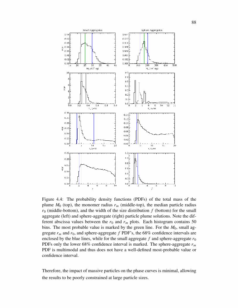
88

Figure 4.4: The probability density functions (PDFs) of the total mass of theplume M0 (top), the monomer radius rm (middle-top), the median particle radiusr0 (middle-bottom), and the width of the size distribution f (bottom) for the smallaggregate (left) and sphere-aggregate (right) particle plume solutions. Note the dif-ferent abscissa values between the r0 and rm plots. Each histogram contains 50bins. The most probable value is marked by the green line. For the M0, small ag-gregate rm and r0, and sphere-aggregate f PDF’s, the 68% confidence intervals areenclosed by the blue lines, while for the small aggregate f and sphere-aggregate r0PDFs only the lower 68% confidence interval is marked. The sphere-aggregate rmPDF is multimodal and thus does not have a well-defined most-probable value orconfidence interval.

Therefore, the impact of massive particles on the phase curves is minimal, allowingthe results to be poorly constrained at large particle sizes.

89

Figure 4.5 gives representative best fits to the VIO (top), CLR (middle), and IR3(bottom) channels of the Cassini ISS data for the small aggregate (red) and sphere-aggregate (green) particle solutions, the latter of which reproduces the lower leftpanel of Figure 6 of IE11. In our case, the small aggregate solution provides thebest fit, as defined by its reduced chi-square value

χ2r =

1N − n − 1

∑i

(xi − µi

)2

σ2i

, (4.10)

where N = 10 is the number of data points being fitted to, n = 4 is the number ofparameters, and the variables in the summation are the same as that of Eq. 4.9.Lower χ2

r values indicate better fits, though if χ2r 1 then the error bars on the

observations are likely overestimated. χ2r = 0.71 for the small aggregate solution

fit and χ2r = 1.5 for the sphere-aggregate solution fit. Both solutions give simi-

lar fits for the VIO and CLR channels, but differ significantly in the IR3 channelat scattering angles < 2. Whereas the small aggregate model curve features abroad forward scattering peak, the sphere-aggregate model curve’s forward scatter-ing peak is much narrower in IR3. The width of the forward scattering peak is re-lated to r0 (IE11), but also rm in the case of aggregates (Lavvas, Yelle, and Griffith,2010); large particles result in narrower/sharper peaks while smaller particles resultin broader peaks. Therefore, as the small aggregate particles have small rm values,their forward scattering peaks are the most broad, increasing R(θ) at larger scatter-ing angles and prompting low M0 values. Meanwhile, the lack of small monomersin the sphere-aggregate particles narrows the forward scattering peak, resulting inlow values at large θ, and a higher M0 than for the small aggregate solution.

It is interesting to note that only the IR3 channel offers a way to discriminate be-tween the two solutions. This is caused by the strong dependence of the intensity ofscattered light on the particle size parameter xm. In our fits there are two ranges ofparticle sizes to consider: the small aggregate monomer radius ∼ 0.3 µ m and themedian particle radius for the small aggregate and sphere-aggregate solutions ∼ 4µm; the intensity of the scattered light will depend on a combination of the particleradius and the monomer radius, if applicable. For the VIO and CLR channels (λ =

420 and 635 nm, respectively), both the small aggregate and sphere-aggregate par-ticles are much larger than the wavelengths considered, leading to narrow forwardscattering peaks. However, for the IR3 channel (λ = 918 nm), the small aggre-gate monomer radius is now much smaller than the wavelength, leading to a much

90

Figure 4.5: Representative best fits to the VIO (top), CLR (middle), and IR3 (bot-tom) wavelength channel data from Cassini ISS for the small aggregate (red) andsphere-aggregate (green) plume particle solutions. Parameters used for the smallaggregate solution fit are: M0 = 22.58 × 103 kg, rm = 0.331 µm, r0 = 3.9 µm, andf = 7.79. Parameters used for the sphere-aggregate solution fit are: M0 = 172.42 ×103 kg, rm = 4.87 µm, r0 = 4.81 µm, and f = 1.71.

broader forward scattering peak. Similarly, the low f value of the sphere-aggregatesolution means that there exists a great number of small particles that are responsi-ble for much of the scattering, and which are now much smaller than the channel

91

wavelength, again leading to a wider forward scattering peak.

In obtaining two separate families of solutions, we have shown that degeneracyexists in the ISS data from IE11 when both spherical and aggregate particles areconsidered. This degeneracy can be broken by an independent mass measurement,such as from Cassini CDA.

4.7 DiscussionWe can calculate the solid to vapor mass ratio of the plume for the small aggregatesolution following the procedure described in IE11. We derive a value for the par-ticulate column mass abundance Mp

col by relating it to the I/F values of the CassiniISS NAC image from IE11 using their Eq. 8,

IF

=Mp

col

M0R(θ) = K0(θ)Mp

col , (4.11)

where R(θ) is defined in Eq. 4.7. Dividing Mpcol by the vapor column mass abun-

dance, Mvcol , at the same altitude above Enceladus then gives the solid to vapor mass

ratio of the plume at that altitude. From the small aggregate curve (red) in Figure4.5, we interpolate a R(θ) value of 6.4 × 103 km2 for the CLR channel at θ = 2.38,the wavelength channel and scattering angle of the NAC image, respectively. Thisis slightly higher than the value given in IE11, 5.4 × 103 km2, owing to the differentmodel curves used for the interpolation. Setting M0 to (25 ± 4) × 103 kg for thesmall aggregate solution and I/F to 0.07, the brightest pixel value of the NAC im-age above background (as with IE11), we find that Mp

col = (2.7 ± 0.4) × 10−7 kg m−2

for that pixel, which is ∼ 7 times lower than the Mpcol value calculated by IE11. The

altitude above Enceladus that corresponds to that pixel is similar to that probed bythe occultations carried out by Hansen et al. (2011) to measure Mv

col using CassiniUVIS. Therefore, the solid to vapor mass ratio can be obtained by dividing the Mp

col

value derived here by the Mvcol value derived from averaging the second column of

Table 1 of Hansen et al. (2011). This gives a solid to vapor mass ratio for the smallaggregate plumes of

Mpcol

Mvcol

= 0.07 ± 0.01, (4.12)

which is again 7 times lower than that of IE11. The error arises from uncertaintiesin both the solid and vapor column mass abundances and is likely underestimated,

92

as we have assumed zero uncertainty for the R(θ = 2.38) and I/F values. It shouldbe noted that, while K0(θ) is defined using all available WAC images, the compar-ison with UVIS requires that we use just the brightest pixel of the one NAC imageto set the I/F value. In other words, the global I/F values of the plume in the WACimages are assumed to be the same as that of the brightest plume pixel in the NACimage, which is equivalent to assuming that the particle size distribution is indepen-dent of altitude above Enceladus. This is only an approximation, as evidence existsthat the particle size distribution does change with altitude (Hedman, Nicholson,et al., 2009; Postberg, Schmidt, et al., 2011). However, for simplicity we do notconsider this effect in this work.

Our calculated solid to vapor ratio is consistent with that of Kieffer, Lu, McFar-quar, et al. (2009), who provided an upper bound of ∼0.1–0.2 using observationsfrom Cassini ISS and UVIS (C. C. Porco et al., 2006). It is also consistent withthe lower end of the range of solid to vapor ratios (∼ 0.01 − −100) calculated byHedman, Nicholson, et al. (2009) using Cassini VIMS observations and sphericaland irregular particle scattering models, though aggregates were not considered.

The K0(θ) quantity in Eq. 4.11 is extremely useful as it can readily convert an ob-served I/F value into the column mass abundance. It also varies depending on theparticle scattering properties, wavelength of scattered light, and particle size dis-tribution. Figure 4.6 shows the K0(θ) values of the small (solid lines) and sphere-aggregate (dashed lines) solutions at scattering angles between 0 and 50 for theVIO (blue), CLR (green), and IR3 (red) wavelength channels. The small aggregateK0(θ) values are, as expected, higher than that of the sphere-aggregate solution,since there is less mass for the same intensity of forward scattering. The sphere-aggregate K0(θ) values are typically within 10% of those of IE11, further reinforc-ing the lack of dependence of the sphere-aggregate solutions on the limitations ofthe T08 model. A full set of K0(θ) values for the two families of solutions and thebest fit solution of IE11 at the Cassini WAC and NAC channel wavelengths can befound in the online supplemental material.

Aside from what can be retrieved from observations, it is also imperative that theparticle solutions are physical and adhere to theoretical constraints of formation andevolution. As IE11 has already considered high mass plumes, we will focus on thelow mass small aggregate solutions and their possible formation mechanisms forthe remainder of this work.

Aggregate particles in the Solar System typically form through the coagulation of

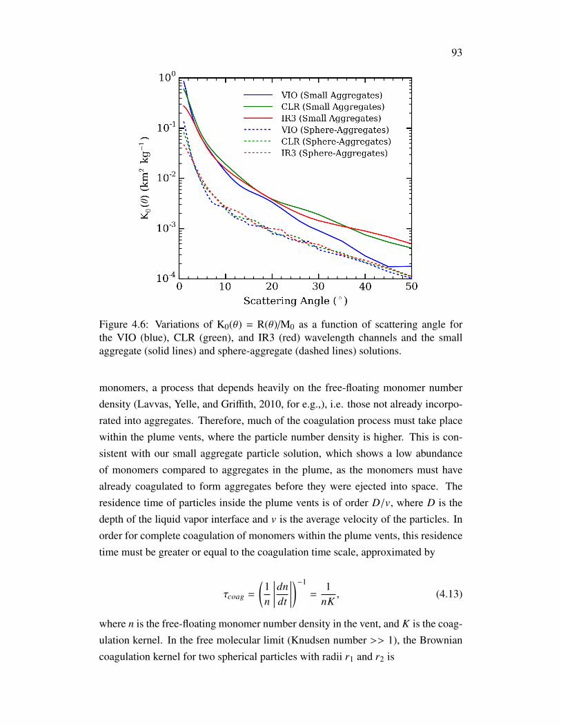
93

Figure 4.6: Variations of K0(θ) = R(θ)/M0 as a function of scattering angle forthe VIO (blue), CLR (green), and IR3 (red) wavelength channels and the smallaggregate (solid lines) and sphere-aggregate (dashed lines) solutions.

monomers, a process that depends heavily on the free-floating monomer numberdensity (Lavvas, Yelle, and Griffith, 2010, for e.g.,), i.e. those not already incorpo-rated into aggregates. Therefore, much of the coagulation process must take placewithin the plume vents, where the particle number density is higher. This is con-sistent with our small aggregate particle solution, which shows a low abundanceof monomers compared to aggregates in the plume, as the monomers must havealready coagulated to form aggregates before they were ejected into space. Theresidence time of particles inside the plume vents is of order D/v, where D is thedepth of the liquid vapor interface and v is the average velocity of the particles. Inorder for complete coagulation of monomers within the plume vents, this residencetime must be greater or equal to the coagulation time scale, approximated by

τcoag =

(1n

dndt

)−1

=1

nK, (4.13)

where n is the free-floating monomer number density in the vent, and K is the coag-ulation kernel. In the free molecular limit (Knudsen number >> 1), the Browniancoagulation kernel for two spherical particles with radii r1 and r2 is

94

K = (r1 + r2)2

√√6kTρp

*,

1r3

1

+1r3

2

+-, (4.14)

where k is the Boltzmann constant, T is temperature, and ρp is the solid particledensity (0.917 g cm−3). Setting r1 = r2 = rm,

K =

√192kTrm

ρp(4.15)

(Pruppacher and Klett, 1978). To find a value for the coagulation time scale, weconsider the rate at which particulate mass is emerging from the vents, which canbe expressed as

dMp

dt=

43πr3

mρpnAv = ρm Av, (4.16)

where ρm is the total mass of particulates per unit volume and A is the total ventarea of the Enceladus plumes. IE11 gives this rate as dMp/dt = 51 kg s−1, butthe reduced plume mass of the small aggregate solutions results in a smaller value.Rather than assuming that dMp/dt is linearly proportional to M0 however, we in-stead appeal to the solid to vapor mass ratio by considering the rate at which vaporis emerging from the vents, dMv/dt, which has been determined by Hansen et al.(2011) to be ∼ 200 kg s−1 based on Cassini UVIS observations. Thus,

dMv

dt= ρv Av = 200 kg s−1, (4.17)

where ρv is the density of the vapor at the liquid-vapor interface, 4.85 × 10−3 kgm−3 at T = 273 K. Dividing Eq. 4.16 by Eq. 4.17 gives us the solid to vapor massratio ∼ [dMp/dt / dMv/dt] and allows us to eliminate A and v. Substituting theresult into Eq. 4.13 then allows us to eliminate n. The necessary condition for thecompletion of monomer coagulation before exiting the vent then becomes

Dv> τcoag =

1K

(43πr3

m

)ρp

ρv

dMv/dtdMp/dt

∼ 20 s, (4.18)

where we use rm = 0.3 µm and T = 273 K. For [dMp/dt / dMv/dt] we use the solidto vapor mass ratio derived in Eq. 4.12.

95

Several assumptions have gone into Eq. 4.18. One is that the particles and thevapor emanate from the same liquid-vapor interface, or at least very close aboveit in the vent. This is necessary to maintain high T and ρp values. If the particlesform in flight higher up in the vent, as in a convective cloud, the reduction in ρp dueto lower T and/or condensation on the vent walls would drastically increase τcoag.The fact that some of the plume particles are Na-rich (Postberg, Kempf, et al., 2009;Postberg, Schmidt, et al., 2011) argues that they originate from the liquid, but wecannot rule out a vapor origin for the Na-poor particles. Another assumption is thatthe different parts of the erupting area A behave the same way whether they are asingle crack running the length of each tiger stripe, a series of 100 discrete sources(C. Porco, DiNino, and Nimmo, 2014), or some combination of the two (Tian et al.,2007; Hansen et al., 2011; Postberg, Schmidt, et al., 2011; Spitale et al., 2015, fore.g.). A third assumption is that the solid to vapor mass ratio remains the sameas the plumes vary with orbitial phase (Hedman, Gosmeyer, et al., 2013). Theseassumptions are difficult to test, but they seem reasonable.

A fourth assumption is that the relevant vapor density and velocity are close to thoseat the liquid-vapor interface and not those at the top of the vent where the particlesand vapor exit to space. From the vertical distribution of particles exiting the vent,one infers velocities of order 60–90 m s−1 (Porco et al., 2006; IE11). However, theparticles are accelerated to this speed within a few meters of the surface (Schmidtet al., 2008; A. P. Ingersoll and Pankine, 2010), so the exit speed underestimatesthe time spent in the vent during which coagulation takes place. Postberg, Kempf,et al. (2009) use 500 m s−1 for the speed of the vapor and the triple point valuefor its density, but Nakajima and A. . Ingersoll (Submitted) point out that these areoverestimates. Their model includes friction with the walls of the crack as the gasflows upward. This produces backpressure at the liquid-vapor interface, and fora long, narrow crack the backpressure severely limits the evaporation rate and theupward velocity. For crack widths less than 0.1 m, the upward velocity is less than10 m s−1 below depths of 1 km. If the evaporating surface is another 1 km below thatlevel, the time spent in the vent is well over 100 s and the condition for coagulationof aggregates (Eq. 4.18) is comfortably satisfied. Crack width is an importantparameter, since it affects the velocity. Nakajima and A. . Ingersoll (Submitted)derive their estimate by matching the ratio of the power released through latentheat to that released through infrared radiation, but one should remember that thesenumbers are uncertain by factors of 2 or more.

96

Our results favor a less violent source for the plumes than the earlier results of IE11.Here, “less violent” means steady, controlled evaporation rather than explosive boil-ing. For example, it could be that most of the ice particles condense directly fromthe expanding vapor above the liquid-vapor interface rather than erupt as a bubblyliquid, which then breaks up and freezes into small ice particles in the vacuum ofspace. Alternatively, the particles could be generated by bubbles of methane or CO2

rising through liquid water and breaking at the surface, thereby sending up a finespray of ice particles. C. C. Porco et al. (2006) mentioned two extremes: parti-cles condensing directly from the vapor and particles forming from the breakup ofa boiling liquid, the latter analogous to a cold Yellowstone geyser. The relativelylarge solid to vapor ratio of IE11 favors the violent source, while the lower ratioof our small aggregate solution allows for less violent sources. Thus, the presentresults make the ISS data compatible with a wider variety of sources than the IE11results.

Schmidt et al. (2008) and A. P. Ingersoll and Pankine (2010) used hydrodynamicmodels to simulate the condensation of ice particles from water vapor, and obtainedsolid to vapor mass ratios of 0.05–0.06 and 0.015, respectively. The lower valuecalculated by A. P. Ingersoll and Pankine (2010) results from the condensation ofvapor onto the vent walls, which Schmidt et al. (2008) did not consider. These val-ues of the solid to vapor mass ratios are more consistent with our small aggregatesolution than with the results of IE11. Kieffer, Lu, Bethke, et al. (2006) consid-ered explosive decomposition of a hydrate clathrate that contains methane and othergases in much greater abundances than their solubility in liquid water would allow.The solid to vapor mass ratio of such an event is uncertain, but it could be lowerthan that quoted by IE11 and closer to the ratio derived here from the small ag-gregate solution. Meanwhile, Hsu et al. (2015) and Postberg, Kempf, et al. (2009)and Postberg, Schmidt, et al. (2011) showed that silica grains and sodium salts arepresent in both E ring and plume particles, which argues strongly for frozen dropletsoriginating from a salty liquid rather than ice particles forming directly from vaporcondensation. Postberg, Kempf, et al. (2009) suggested that ascending bubbles ofplume gases (CO2, N2, CO, CH4) can disperse the liquid droplets into the vapor,and that the evaporation of the boiling liquid source is taking place over a large hor-izontal area so that freezing of the vents is suppressed. Nakajima and A. . Ingersoll(Submitted) showed that the backpressure due to friction on the walls of the channelcould severely limit the evaporation rate. A. P. Ingersoll and Nakajima (Submitted)argue that this “controlled boiling” allows bubbles of vapor to break at the surface

97

instead of throwing up large amounts of spray as in boiling into vacuum. All of thispoints to a relatively gentle source and a relatively low solid to vapor mass ratio.

Our small aggregate solution does not rule out a vapor-based source for the plumeparticles. Parkinson et al. (2008) showed that spherical particles with radii similarto rm can form from water vapor nucleating on involatile grains in a few seconds,while spherical particles with radii up to 3 µm can form by condensation in about100 s, though large condensation nuclei and/or a high density of water vapor maybe necessary. Similarly, non-spherical ice crystals resembling aggregates, e.g. den-dritic shapes, can form directly from condensation and nucleation of water vapor,with growth rates comparable to that of spherical particles (Pruppacher and Klett,1978). Bullet rosettes – highly non-spherical, polycrystalline ice particles made upof clumps of hexagonal columns – can also yield high scattering cross sections for asmall particle mass, but they are formed by the fracturing of ice during the freezingof a large water drop (Baum et al., 2011).

We have shown that forward scattering observations of the Enceladus plumes fromCassini ISS can be well-fit by plumes made up of ice aggregates and solid icespheres. This results in a bifurcation in the allowed total particulate mass of theplumes: small aggregate plumes are six times less massive than plumes made oflarger aggregates and spheres. The small aggregate plumes, in particular, lead to asolid to vapor mass ratio of 0.07 ± 0.01, which is suggestive of a “gentle source”for the plume particles.

We thank Y. L. Yung and H. Ngo for their valuable input. P. Gao and P. Kop-parla were supported in part by an NAI Virtual Planetary Laboratory grant fromthe University of Washington to the Jet Propulsion Laboratory and California In-stitute of Technology under solicitation NNH12ZDA002C and Cooperative Agree-ment Number NNA13AA93A. X. Zhang was supported by the Bisgrove ScholarProgram at the University of Arizona. A. P. Ingersoll was supported by the CassiniProject and NASA’s Cassini Data Analysis Program.

References

Bar-Nun, A., V. Dimitrov, and M. G. Tomasko (2008). “Titan’s aerosols: Compari-son between our model and DISR findings”. In: Planetary and Space Science 56,pp. 708–714.

Baum, B. A. et al. (2011). “Improvements in shortwave bulk scattering and ab-sorption models for the remote sensing of ice clouds”. In: Journal of AppliedMeteorology and Climatology 50, pp. 1037–1056.

98

Botet, R., P. Rannou, and M. Cabane (1997). “Mean-field approximation of Miescattering by fractral aggregates of identical spheres”. In: Applied Optics 36,pp. 8791–8797.

Cabane, M. et al. (1993). “Fractal aggregates in Titan’s atmosphere”. In: Planetaryand Space Science 41, pp. 257–267.

Coustenis, A. et al. (2001). “Images of Titan at 1.3 and 1.6 µm with adaptive opticsat the CFHT”. In: Icarus 154, pp. 501–515.

Grainger, R. G. et al. (2004). “Calculation of Mie derivatives”. In: Applied Optics43, pp. 5386–5393.

Hansen, C. J. et al. (2011). “The composition and structure of the Enceladus plume”.In: Geophysical Research Letters 38.

Hastings, W. K. (1970). “Monte Carlo sampling methods using Markov chains andtheir applications”. In: Biometrika 57, pp. 97–109.

Hedman, M. M., C. M. Gosmeyer, et al. (2013). “An observed correlation betweenplume activity and tidal stresses on Enceladus”. In: Nature 500, pp. 182–184.

Hedman, M. M., P. D. Nicholson, et al. (2009). “Spectral observations of the Ence-ladus plume with Cassini-VIMS”. In: The Astrophysical Journal 693, p. 1749.

Heymsfield, A. J. et al. (2002). “A general approach for deriving the properties ofcirrus and stratiform ice cloud particles”. In: Journal of the atmospheric sciences59, pp. 3–29.

Hsu, H. W. et al. (2015). “Ongoing hydrothermal activities within Enceladus”. In:Nature 519, pp. 207–210.

Ingersoll, A. P. and S. P. Ewald (2011). “Total particulate mass in Enceladus plumesand mass of Saturn’s E ring inferred from Cassini ISS images”. In: Icarus 216,pp. 492–506.

Ingersoll, A. P. and M. Nakajima (Submitted). “Controlled boiling on Enceladus. 2.Model of the liquid-filled cracks”. In: Icarus.

Ingersoll, A. P. and A. A. Pankine (2010). “Subsurface heat transfer on Enceladus:Conditions under which melting occurs”. In: Icarus 206, pp. 594–607.

Kajikawa, M. and A. J. Heymsfield (1989). “Aggregation of ice crystals in cirrus”.In: Journal of the Atmospheric Sciences 46, pp. 3108–3121.

Kieffer, S. W., X. Lu, C. M. Bethke, et al. (2006). “A clathrate reservoir hypothesisfor Enceladus’ south polar plume”. In: Science 314, pp. 1764–1766.

Kieffer, S. W., X. Lu, G. McFarquar, et al. (2009). “A redetermination of the ice/vaporratio of Enceladus’ plumes: Implications for sublimation and the lack of a liquidwater reservoir”. In: Icarus 203, pp. 238–241.

99


Meng, Z. et al. (2010). “Single-scattering properties of tri-axial ellipsoidal mineraldust aerosols: A database for application to radiative transfer calculations”. In:Journal of Aerosol Science 41, pp. 501–512.

Mishchenko, M. I., L. D. Travis, and D. W. Mackowski (1996). “T-matrix com-putations of light scattering by nonspherical particles: A review”. In: Journal ofQuantitative Spectroscopy and Radiative Transfer 55, pp. 535–575.

Nakajima, M. and A .P. Ingersoll (Submitted). “Controlled boiling on Enceladus. 1.Model of the vapor-driven jets”. In: Icarus.

Parkinson, C. D. et al. (2008). “Habitability of Enceladus: Planetary conditions forlife”. In: Origins of Life and Evolution of Biospheres 38, pp. 355–369.

Porco, C. C. et al. (2006). “Cassini observes the active south pole of Enceladus”.In: Science 311, pp. 1393–1401.

Porco, C., D. DiNino, and F. Nimmo (2014). “How the geysers, tidal stresses andthermal emission across the south polar terrain of Enceladus are related”. In: TheAstronomical Journal 148, pp. 45–68.

Postberg, F., S. Kempf, et al. (2009). “Sodium salts in E-ring ice grains from anocean below the surface of Enceladus”. In: Nature 459, pp. 1098–1101.

Postberg, F., J. Schmidt, et al. (2011). “A salt-water reservoir as the source of acompositionally stratified plume on Enceladus”. In: Nature 474, pp. 620–622.


Rannou, P., T. Cours, et al. (2010). “Titan haze distribution and optical propertiesretrieved from recent observations”. In: Icarus 208, pp. 850–867.

Rannou, P., F. Hourdin, and C. P. McKay (2002). “A wind origin for Titan’s hazestructure”. In: Nature 418, pp. 853–856.

Rannou, P., F. Hourdin, C. P. McKay, and D. Luz (2004). “A coupled dynamics-microphysics model of Titan’s atmosphere”. In: Icarus 170, pp. 443–462.

Rannou, P., C. P. McKay, et al. (1999). “Semi-empirical model of absorption andscattering by isotropic fractal aggregates of spheres”. In: Planetary and SpaceScience 47, pp. 385–396.

Schmidt, J. et al. (2008). “Slow dust in Enceladus’ plume from condensation andwall collisions in tiger stripe fractures”. In: Nature 451, pp. 685–688.

Schmitt, C. G. and A. J. Heymsfield (2010). “The dimensional characteristics ofice crystal aggregates from fractal geometry”. In: Journal of the AtmosphericSciences 67, pp. 1605–1616.

100

Spitale, J. N. et al. (2015). “Curtain eruptions from Enceladus’ south-polar terrain”.In: Nature 521, pp. 57–60.

Tian, F. et al. (2007). “Monte Carlo simulations of the water vapor plumes on Ence-ladus”. In: Icarus 188, pp. 154–161.

Tomasko, M. G., L. Doose, L. E. Dafoe, et al. (2009). “Limits on the size of aerosolsfrom measurements of linear polarization in Titan’s atmosphere”. In: Icarus 204,pp. 271–283.

Tomasko, M. G., L. Doose, S. Engel, et al. (2008). “A model of Titan’s aerosolsbased on measurements made inside the atmosphere”. In: Planetary and SpaceScience 56, pp. 669–707.

Vahidinia, S. et al. (2011). “Saturn’s F-ring grains: Aggregates made of crystallinewater ice”. In: Icarus 215, pp. 682–694.

Waite Jr, J. H. et al. (2009). “Liquid water on Enceladus from observations of am-monia and 40Ar in the plume”. In: Nature 460, pp. 487–490.


Westbrook, C. D., R. C. Ball, and P. R. Field (2006). “Radar scattering by aggre-gate snowflakes”. In: Quarterly Journal of the Royal Meteorological Society 132,pp. 897–914.

Xu, Y. I. (1995). “Electromagnetic scattering by an aggregate of spheres”. In: Ap-plied Optics 34, pp. 4573–4588.

Yang, P. and K.-N. Liou (1998). “Single-scattering properties of complex ice crys-tals in terrestrial atmosphere”. In: Beitrage zur Physik der Atmosphare-Contributionsto Atmospheric Physics 71, pp. 223–248.

Zhang, X. et al. (2013). “Stratospheric aerosols on Jupiter from Cassini observa-tions”. In: Icarus 226, pp. 159–171.

101

PART III: STRANGE NEW WORLDS

102

C h a p t e r 5

MICROPHYSICS OF KCL AND ZNS CLOUDS ON GJ 1214 B

5.1 AbstractClouds have been shown to be ubiquitous in warm exoplanet atmospheres, par-ticularly Super Earths and Mini Neptunes, where they block the spectral signa-tures of key atmospheric molecules in the transmission spectra of exoplanets. Notonly does this prevent us from gaining knowledge about their atmospheric compo-sition, but also require that we include clouds in their atmospheric models in orderto fully characterize them. The formation and evolution of clouds are controlledby microphysical processes, including nucleation, condensation/evaporation, andtransport, which have not yet been incorporated into exoplanet cloud models thatcan simulate worlds smaller and cooler than Hot Jupiters. In this work, we ap-ply a cloud microphysics model to simulate the potassium chloride (KCl) and zincsulfide (ZnS) clouds of the Super Earth GJ 1214 b. We investigate the cloud dis-tribution as a function of the degree of vertical mixing, as parameterized by eddydiffusion, and the atmospheric metallicity. We find that pure ZnS clouds do notform via homogeneous nucleation because of its high surface energy, and when itis allowed to heterogeneously nucleate onto KCl particles it remains a minor cloudcomponent. Pure KCl cloud distributions are strongly influenced by the rates of ho-mogeneous nucleation versus the rates of sedimentation/mixing and condensationalgrowth. High eddy diffusivities promote high rates of nucleation due to increasedupwelling of KCl vapor from depth and generate more massive, vertically extendedclouds, while low eddy diffusivities lead to diminutive clouds that experience peri-odic bursts of nucleation. Higher metallicities drastically increase the cloud massdue to higher supersaturations leading to high nucleation rates, and as a result evenmoderately supersolar metallicities (0 < [Fe/H] < 1) may produce optically thickclouds at high altitudes. Possible cloud nucleation pathways are discussed, whichwill require laboratory work into exoplanet cloud material properties to be fullyunderstood.

5.2 IntroductionInvestigations of exoplanet atmospheres have unearthed a prevalence of clouds andhazes that impede understanding of atmospheric composition (Gibson, Aigrain,

103

Pont, et al., 2012; Gibson, Aigrain, Barstow, et al., 2013; Deming et al., 2013;Jordán et al., 2013; Mandell et al., 2013; Sing, Lecavelier des Etangs, et al., 2013;Chen et al., 2014; Schlawin et al., 2014; Wilkins et al., 2014; Fukui et al., 2014;Mallonn and Strassmeier, 2016). Their presence is typically revealed through aflattening of spectral features in the transmission spectrum, resulting from the in-ability of stellar photons to reach depths in the atmosphere below the cloud top dueto scattering and absorption by the cloud particles. This phenomenon is observedacross many exoplanets of various sizes, effective temperatures, and stellar irradi-ation levels. For example, while many super Earths and warm Neptunes appearcloudy (e.g. Crossfield et al., 2013; Kreidberg et al., 2014; Knutson, Benneke, etal., 2014; Knutson, Dragomir, et al., 2014), there exist exceptions (Fraine et al.,2014). Meanwhile, a continuum in cloudiness has been observed for hot Jupiters(Sing, Fortney, et al., 2016; Iyer et al., 2016), as determined from the magnitude ofthe spectral features of water, potassium, sodium, and Rayleigh scattering.

There are now some hints of correlations between cloudiness and other planetaryproperties, such as geometric albedo and equilibrium temperature (Heng and De-mory, 2013; Stevenson, 2016), but the processes that control the formation and dis-tribution of exoplanet clouds are still mostly unknown. This is a profound problem,as clouds are strongly coupled to the atmospheric radiation environment, chemicalcomposition, and dynamics. For example, the presence of a cloud formed from con-densation gives clues to the temperature structure and metallicity of an atmosphere,as cloud formation requires a supersaturation of the condensing species. In addi-tion, clouds obfuscate investigations of exoplanet atmospheres by hiding molecularspectral features, and thus future exoplanet observing missions and programs wouldgreatly benefit from a theoretical framework that can determine a priori whether anexoplanet is cloudy or clear.

Previous efforts in detailed modeling of exoplanet clouds can be split into two cat-egories: Equilibrium condensation and grain chemistry. Equilibrium condensationpresumes an atmosphere with a composition determined by thermochemical equi-librium, and that certain species can be in their condensed phase if it is energeti-cally favorable. The resulting condensed material would be distributed verticallysuch that the sedimentation of cloud particles is balanced by vertical lofting due toeddy mixing (A. S. Ackerman and Marley, 2001). Using this framework, Morley,Fortney, Marley, Visscher, et al. (2012) showed that the formation of sulfide clouds(e.g. Na2S) could explain the infrared colors of cooler Brown dwarfs, while Morley,

104

Fortney, Kempton, et al. (2013) was able to explain the flat transmission spectrumof the super Earth GJ 1214 b by appealing to the formation of KCl and ZnS cloudsin a high (100–1000 times solar) metallicity atmosphere. Charnay, Meadows, andLeconte (2015) and Charnay, Meadows, Misra, et al. (2015) extended this schemeto 3D and found that submicron KCl and ZnS particles can be lofted to high enoughaltitudes such that the resulting transmission spectrum is flat within the uncertain-ties of the data. However, while these models have been successful in explainingthe available data, they lack the physical processes that govern cloud formationand evolution on the scale of the particles, namely their initial nucleation and theirsubsequent growth/loss through microphysical processes. This deficiency dampenstheir predictive powers.

In contrast to the equilibrium condensation models, grain chemistry models as-sume that cloud formation is a kinetics process, characterized by the growth andshrinking of cloud particles with mixed compositions via heterogeneous chemicalreactions on their surfaces. This framework has been developed in great detail forbrown dwarf and hot Jupiter atmospheres, where the cloud formation processes isassumed to begin with the nucleation of TiO2 clusters in the upper atmospherethat are then transported downwards and act as nucleation sites for an array ofcondensing species, including MgSiO3, Mg2SiO4, SiO2 ,Al2O3, and Fe (Helling,Oevermann, et al., 2001; Woitke and Helling, 2003; Woitke and Helling, 2004;Helling, Klein, et al., 2004; Helling and Woitke, 2006; Helling, A. Ackerman, etal., 2008; Helling, Woitke, and Thi, 2008; Witte, Helling, and Hauschildt, 2009;Witte, Helling, Barman, et al., 2011; Lee, Helling, Dobbs-Dixon, et al., 2015; Lee,Helling, Giles, et al., 2015; Helling, Lee, et al., 2016). These models have beencompared favorably to brown dwarf emission spectra (Witte, Helling, Barman, etal., 2011), and have shown that a vertical gradient in cloud composition is likely inbrown dwarf and hot exoplanet atmospheres. In addition, these models have alsobeen recently extended to 3D (Lee, Helling, Dobbs-Dixon, et al., 2015; Helling,Lee, et al., 2016), and showed that HD 189733b and HD 209458b are envelopedby mineral clouds with vertical and latitudinal variations in composition due todynamics and global temperature differences, with the former planet exhibiting alower cloud deck, explaining the more pronounced molecular features in its trans-mission spectra. Though these models have greatly illuminated the complexities ofbrown dwarf/exoplanet cloud processes, they are difficult to generalize due to theirreliance on the specific TiO2 nucleation pathway for cloud formation. As a result,they have not yet been used to investigate cooler, smaller exoplanets.

105

In this work we explore the formation and evolution of exoplanet clouds from aperspective especially applicable to cooler atmospheres: cloud microphysics. OnEarth, water clouds form through condensation of preexisting water molecules ontocondensation nuclei (heterogeneous nucleation) or, less frequently, by homoge-neous nucleation where no seeds are necessary; these cloud particles can then growby condensation and coagulation/coalescence, or shrink by evaporation, and aretransported through sedimentation, advection, and turbulent mixing. These pro-cesses are likely at work across the Solar System, controlling the sulfuric acidclouds of Venus (Gao et al., 2014), the CO2 and water clouds of Mars (Michelangeliet al., 1993; Colaprete, Toon, and Magalhães, 1999), the ammonia clouds of Jupiterand Saturn (Rossow, 1978; Carlson, Rossow, and Orton, 1988), and the hydrocar-bon clouds of Titan, Uranus, and Neptune (Moses, Allen, and Yung, 1992; Barthand Toon, 2003; Barth and Toon, 2004; Barth and Toon, 2006). Cloud microphysicsis a variation on grain chemistry in that it also treats cloud formation as a kineticsprocess, but it presumes that the condensing material already exists as free floatingmolecules, whereas in grain chemistry many of the condensed species form on thegrains themselves.

We use the 1–dimensional Community Aerosol and Radiation Model for Atmo-spheres (CARMA), which calculates the rates of particle growth and loss due to theaforementioned cloud microphysics processes. We apply our model to GJ 1214 b,as it has the highest precision observations for planets in its size and temperaturerange (Kreidberg et al., 2014), and simulate the formation of KCl and ZnS clouds.Not only does this allow us to test our model in an exoplanet framework, but we willalso be able to investigate the assumptions and results of previous studies that havetargeted this world (Morley, Fortney, Kempton, et al., 2013; Charnay, Meadows,and Leconte, 2015; Charnay, Meadows, Misra, et al., 2015).

In §5.3, we describe our cloud microphysics model, including the augmentationsneeded to simulate exoplanet clouds. We discuss our results in §5.4, where weshow how the cloud distribution varies with atmospheric mixing and metallicity,and when composite cloud particles are allowed. We present our conclusions andmake recommendations for future investigations in §5.6.

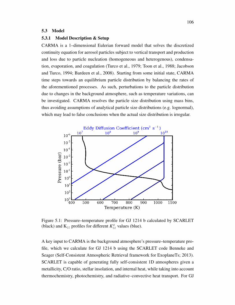
106

5.3 Model5.3.1 Model Description & SetupCARMA is a 1–dimensional Eulerian forward model that solves the discretizedcontinuity equation for aerosol particles subject to vertical transport and productionand loss due to particle nucleation (homogeneous and heterogenous), condensa-tion, evaporation, and coagulation (Turco et al., 1979; Toon et al., 1988; Jacobsonand Turco, 1994; Bardeen et al., 2008). Starting from some initial state, CARMAtime steps towards an equilibrium particle distribution by balancing the rates ofthe aforementioned processes. As such, perturbations to the particle distributiondue to changes in the background atmosphere, such as temperature variations, canbe investigated. CARMA resolves the particle size distribution using mass bins,thus avoiding assumptions of analytical particle size distributions (e.g. lognormal),which may lead to false conclusions when the actual size distribution is irregular.

Figure 5.1: Pressure–temperature profile for GJ 1214 b calculated by SCARLET(black) and Kzz profiles for different Ko

zz values (blue).

A key input to CARMA is the background atmosphere’s pressure–temperature pro-file, which we calculate for GJ 1214 b using the SCARLET code Benneke andSeager (Self-Consistent Atmospheric Retrieval framework for ExoplaneTs; 2013).SCARLET is capable of generating fully self-consistent 1D atmospheres given ametallicity, C/O ratio, stellar insolation, and internal heat, while taking into accountthermochemistry, photochemistry, and radiative–convective heat transport. For GJ

107

1214 b we generated pressure–temperature profiles for a clear, H/He-dominated at-mosphere in radiative–convective equilibrium, which we split into 80 levels (Figure5.1). The atmospheric compositions is assumed to be in thermochemical equilib-rium with solar C/O ratios and metallicities of 1×, 10×, and 100× solar metallicity(i.e. [Fe/H] = 0, 1, 2). Morley, Fortney, Kempton, et al. (2013) showed that increas-ing metallicity leads to cloud decks of higher optical depth, and we will test thisresult using our model, and evaluate how cloud optical depth scales with metallic-ity. In addition, we test multiple values for the eddy diffusivity, Kzz , parameterizedaccording to Charnay, Meadows, and Leconte (2015),

Kzz = Kozz P−0.4, (5.1)

where P is the atmospheric pressure in bars, and Kozz is set to 107, 108, 109, and

1010 cm2 s−1 in our tests. Figure 5.1 shows these Kzz profiles. Note that we limiteditheir values to below 1010 cm2 s−1 at all pressure levels. For comparison, Charnay,Meadows, and Leconte (2015) found values for Ko

zz between 7 × 106 and 3 × 107

cm2 s−1 in their GCM simulations.

Abundances of the condensates, KCl and ZnS, were assumed to correspond to thoseof K and Zn at the designated metallicities, as they are both the least abundantelement in their molecules. In other words, we assume that all K is tied up in KCland all Zn in ZnS. The volume mixing ratios of K and Zn in an atmosphere of H2

and He at solar metallicity are 0.22 and 0.076 ppmv, respectively Lodders (2010).

All simulations are initiated in an atmosphere devoid of particles, and with con-stant KCl and ZnS volume mixing ratios at all pressure levels corresponding totheir 1×, 10×, or 100× metallicity abundances. Both species are then allowed tohomogeneously nucleate to produce cloud particles, and evolve towards equilib-rium. For one simulation we allow ZnS to both homogeneously nucleate and het-erogeneously nucleate on homogeneously nucleated KCl cloud particles, producinglayered, mixed clouds. Once formed, the cloud particles are transported via eddydiffusion and sedimentation under gravity, with a gravitational acceleration for GJ1214 b of 8.93 m s−2 (Charbonneau et al., 2009). We set a zero–flux top boundarycondition, corresponding to a lack of significant loss of condensing/condensed ma-terial to space. For the bottom boundary, we hold the abundances of KCl and ZnSvapor to their initial values, and set the particle abundance to zero, as the condensatevapors are vastly undersaturated there.

108

Condensational growth in CARMA takes into account latent heating of particlesdue to the addition of vapor molecules. This heat is removed from the particle byconduction. We set the thermal conductivity κ of the atmosphere to be that of pureH2, given by

κ(ergs s−1 m−1 K−1) = 7148.57 + 39.12T + 3.1607 × 10−3T2, (5.2)

where T is temperature (in K) and the numerical coefficients are obtained by fittingto data from Lemmon (2016). For the heat capacity of the atmosphere Cp, which isused to correct for κ in the kinetics limit, we use a constant value of 1.3 × 108 ergsg−1 K−1, appropriate for a H2–dominated atmosphere (Kataria et al., 2015). Theviscosity of the atmosphere is given by the Sutherland equation

η(Poise) = 8.76 × 10−5(

293.85 + 72T + 72

) (T

293.85

)1.5

, (5.3)

where the numerical constants are those for H2 taken from White (1974). Theatmospheric viscosity is needed to calculate the sedimentation velocity of cloudparticles in the continuum limit.

5.3.2 Microphysical Properties of KCl & ZnSAnother set of key inputs to CARMA are the material properties that define eachcondensing species, including their densities (1.98 g cm−3 for KCl and 4.09 g cm−3

for ZnS), saturation vapor pressures, surface tensions/energies, latent heats, andmolecular diffusion coefficients.

The saturation vapor pressures Psx for KCl and ZnS have been estimated from by

Morley, Fortney, Marley, Visscher, et al. (2012) to be

log PsKCL = 7.611 − 11382/T (5.4)

log PsZnS = 12.812 − 15873/T − [Fe/H], (5.5)

where Psx is in bars. These saturation vapor pressures can then be used in conjunc-

tion with the Clausius–Clapeyron equation

d ln Psx

dT=

LRT2 (5.6)

109

to calculate the latent heats L, where R is the universal gas constant. For KCl andZnS, L is found to be 2.923 × 1010 ergs g−1 and 3.118 × 1010 ergs g−1, respectively(Charnay, Meadows, Misra, et al., 2015).

The surface tension γx of molten KCl is (Janz and Dijkhuis, 1969)

γKCl (ergs cm−2) = 160.4 − 0.07T. (5.7)

This value is similar to that found for the 100 face of solid KCl crystals (West-wood and Hitch, 1963), which is reassuring since it is unknown what phase KClwould be in exoplanet atmospheres. No data exists regarding the surface tensionof liquid ZnS, so we use the surface energy of ZnS solid, γZnS = 1672 ergs cm−2

(Celikkaya and Akinc, 1990). Note the one order of magnitude difference betweenKCl and ZnS; as the particle nucleation and condensation rates scale exponentiallywith surface energy to the third power, this will likely have a large impact on theresulting cloud structure.

Condensation of trace gases in an atmosphere depends strongly on the diffusion rateof gas molecules to the cloud particles. The molecular diffusion coefficient D canbe expressed using Chapman–Enskog theory as (Jacobson, 2005)

D =5

16Ad2ρaΩc

√RT µa (µc + µa)

2πµc, (5.8)

where A is Avogadro’s number, ρa is the atmospheric mass density, µa and µc arethe mean molecular weight of the atmosphere and molecular weight of the condens-ing species, respectively, Ωc is the collision integral of the condensing species withthe main atmospheric components and is of order unity, and d is the collision di-ameter of the condensing species. We estimate the collision diameters for KCl andZnS to be 2.67 Å and 2.0464 Å, respectively, from their equilibrium bond lengths(Sanderson, 1976; Zack and Ziurys, 2009).

For our test case where ZnS is allowed to nucleate on KCl, an additional set ofphysical quantities that relate the two species must be known. These include thecontact angle made by the surface of a ZnS “droplet” on the surface of a KCl grain,which is related to the surface energies of the two species against the atmosphereand the interfacial energy of the two species together; the desorption energy of aZnS molecule on a KCl surface; and the oscillation frequency associated with said

110

desorption energy. None of these quantities are known at present, and would requirelaboratory investigations to measure. We have thus made approximations for theirvalues. The desorption energy and associated oscillation frequency have been setto that of water over silicate surfaces, 0.18 eV and 1013 Hz, respectively (Lavvas,Griffith, and Yelle, 2011). The contact angle is completely unknown, and so wehave set it to a small value of 2 to promote formation of layered clouds. Increasingthis angle would decrease the rate at which ZnS nucleate onto KCl, and vice versa.Once ZnS has nucleated onto the KCl particle, it is assumed to completely coverit, thereby cutting off KCl vapor from condensing onto the KCl “core”. This isdifferent from the approach of Helling and Woitke (2006) and similar models, wheremultiple condensates can condense on a particle simultaneously.

5.4 Results5.4.1 The Lack of Pure ZnS CloudsNo pure ZnS clouds resulted from our microphysical calculations due to its lowhomogeneous nucleation rates stemming from its high surface energy. Thus, theequilibrium cloud distributions we present in §5.4.2 and §5.4.3 are those of KClonly. Our results are in contrast with the results of equilibrium condensation cloudmodels, which show ZnS to be a major cloud component on warm super Earths(Morley, Fortney, Kempton, et al., 2013; Morley, Fortney, Marley, Zahnle, et al.,2015). We will discuss how ZnS can still manifest as a cloud material in §5.4.4.

5.4.2 Variations with Kzz

Figure 5.2 shows the total particle number density (solid) and total condensed massdensity (dashed) for the resulting cloud distribution at equilibrium subject to eddydiffusion coefficients at 1 bar of 107 (red), 108 (yellow), 109 (green), and 1010 cm2

s−1 (blue). Solar metallicity is assumed. Both the number of cloud particles and thecondensed mass generally increase with increasing eddy diffusion coefficient, butthe increase is not linear, suggesting contributions from processes beyond verticaltransport (see below). Furthermore, the peaks in the particle number density curvesoccur higher in the atmosphere than the peaks of the mass density curves, suggest-ing that most of the mass contribution comes from large particles at the cloud base.

Figure 5.3 shows the particle size distribution at 0.1 bar in the atmosphere corre-sponding to the four eddy diffusion cases (same colors as in Figure 5.2). None ofthe distributions are strictly lognormal, as has been proposed for previous exoplanetcloud models (e.g. A. S. Ackerman and Marley, 2001), and they evolve further away

111

Figure 5.2: Particle number density (solid) and mass density of condensed material(dashed) as a function of atmospheric pressure level for Ko

zz values of 107 (red), 108

(yellow), 109 (green), and 1010 cm2 s−1 (blue). Solar metallicity is assumed.

Figure 5.3: Particle size distributions at 0.1 bars in the atmosphere. The colorsindicate the same Ko

zz values as in Figure 5.2.

from lognormal as Kzz is increased. At the highest Kzz , the distribution is nearlyflat from 10 nm to several microns. This is indicative of a blending of two or more

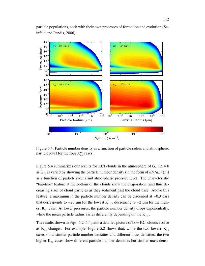
112

particle populations, each with their own processes of formation and evolution (Se-infeld and Pandis, 2006).

Figure 5.4: Particle number density as a function of particle radius and atmosphericparticle level for the four Ko

zz cases.

Figure 5.4 summarizes our results for KCl clouds in the atmosphere of GJ 1214 bas Kzz is varied by showing the particle number density (in the form of dN/dLn(r))as a function of particle radius and atmospheric pressure level. The characteristic“bar–like” feature at the bottom of the clouds show the evaporation (and thus de-creasing size) of cloud particles as they sediment past the cloud base. Above thisfeature, a maximum in the particle number density can be discerned at ∼0.3 barsthat corresponds to ∼20 µm for the lowest Kzz , decreasing to ∼2 µm for the high-est Kzz case. At lower pressures, the particle number density drops exponentially,while the mean particle radius varies differently depending on the Kzz .

The results shown in Figs. 5.2–5.4 paint a detailed picture of how KCl clouds evolveas Kzz changes. For example, Figure 5.2 shows that, while the two lowest–Kzz

cases show similar particle number densities and different mass densities, the twohigher Kzz cases show different particle number densities but similar mass densi-

113

ties. Meanwhile, Figure 5.3 shows that the lowest Kzz case has a nearly lognormalsize distribution, while the higher Kzz cases have particle size distributions moreextended towards smaller radii. Finally, Figure 5.4 show that, for the lowest Kzz

case, the mean particle radius drops precipitously to smaller values higher up in thecloud, while higher Kzz cases maintain a healthy supply of large particles even athigh altitudes. These results suggest that there are two regimes of cloud formationin this system, and it is likely related to the interplay between transport and particleformation via homogeneous nucleation.

In the first regime, corresponding to low Kzz values, the upwelling rate of KCl vaporfrom depth is low, producing small supersaturations in the cloud–forming regionright above the cloud base, which in turn leads to low rates of particle productionvia homogeneous nucleation. The main particle population is therefore an “aged”population sustained by upward lofting and condensation growth, while undergoingsedimentation at the same time. These processes combined result in lognormal sizedistributions. The two lowest–Kzz cases correspond to this regime.

As Kzz is increased, the rate at which KCl vapor is upwelled from depth into thecloud forming region near the cloud base also increases. This leads to higher su-persaturations and higher rates of particle nucleation, which preferentially producenumerous smaller particles, leading to the extension of the particle size distributionsto smaller particle radii and higher particle number densities. These smaller parti-cles take longer to sediment, thus increasing the cloud mass as well. At the sametime, increased mixing leads to higher lofting of large particles, thereby increasingthe presence of large particles at higher altitudes. The two higher Kzz cases corre-spond to this regime, which is sustained by homogeneous nucleation and mixing.

The two lowest–Kzz cases have a further property not shown in the previous fig-ures, in that their cloud distributions oscillate in time. This is shown in Figure 5.5,where we present the time evolution of the cloud mass density (top 2 plots), parti-cle number density (middle two plots), and KCl vapor saturation radio (= the ratioof the KCl partial pressure to its saturation vapor pressure; bottom two plots). Amajor difference between the two lowest–Kzz cases is the period of this oscillation,with the higher Kzz case (lower plot of each pair) oscillating ∼7 times faster. Thisoscillation likely results from the homogeneous nucleation occurring in this regimeof cloud formation.

At equilibrium, most of the cloud particles are growing by condensation and sed-imenting out of the cloud deck, with very low rates of homogeneous nucleation

114

Figure 5.5: Time evolution of the condensed mass density (top two), particle num-ber density (middle two), and KCl saturation ratio (bottom two) for the Ko

zz = 107

(top of each pair) and 108 (bottom of each pair) cases.

creating new particles. The cloud can eventually be depleted in this manner, asthe Kzz is not high enough to sustain large particles, which all particles eventuallyevolve towards due to constant condensational growth resulting from a steady sup-ply of KCl vapor from depth. However, as the cloud is depleted, the rate of KClvapor uptake by the particles also decrease. Eventually, the condensation rate be-

115

comes lower than the KCl vapor upwelling rate, and the vapor mixing ratio beginsto increase. Though this may lead to increased growth, the resulting larger particleswill simply sediment faster, further decreasing the vapor uptake by the cloud par-ticles. At the same time, as the KCl vapor increases in the cloud forming region,the rate of homogeneous nucleation increases exponentially, eventually reaching acritical value (i.e. the rate of vapor uptake due to particle formation balances theinflux of vapor from depth) where the increased particle formation depletes the KClvapor. Particle formation then decreases to very low values once more, and thenewly created particles begin growing by condensation eventually sediment out ofthe cloud, thus completing the cycle.

The above sequence can be seen in Figure 5.5 by tracing how the KCl saturationratio correlates with the particle number density and condense mass density. For ex-ample, in the lowest Kzz case, the saturation ratio reaches a maximum in the cloudformation region (∼0.01 bar) at ∼1.05 × 109 s, at which time both particle densi-ties make sudden jumps to their maximum values. The KCl vapor is then quicklydepleted while the particle densities begin a slow decline as the new particles growand sediment out of the cloud. Eventually, as the condensation centers are depleted,the KCl saturation ratio begins to increase again.

The processes described above is heavily dependent on the rate at which KCl is sup-plied to the cloud forming regions. Increasing this rate leads to increased rates ofparticle growth and depletion, and thus increased frequency of oscillation, which iswhat is seen in our results when the two lowest Kzz cases are compared. However,this sequence eventually breaks down when the “background” homogeneous nucle-ation rate becomes comparable to the particle growth and sedimentation rates. Inother words, this oscillatory behavior should be significantly reduced for the higherKzz regimes. Figure 5.6 shows that this is indeed the case, though oscillations withcomparatively tiny amplitudes still persist.

It is useful to evaluate whether this oscillatory behavior is important for exoplanetclouds. The time scales are long: 7 Earth years for the lowest Kzz case and 1Earth year for the next highest Kzz case. This is far longer than timescales asso-ciated with atmospheric dynamics (e.g. Charnay, Meadows, and Leconte, 2015),which can potentially produce local pockets of supersaturation that causes high ho-mogeneous nucleation rates (Helling, Oevermann, et al., 2001). Two possibilitiesexist: (1) the oscillations seen here occur over a long time scale, on top of the shorttimescale cloud variations due to dynamics, or (2) atmospheric dynamics disrupt

116

Figure 5.6: Same as Figure 5.5 for the Kozz = 109 (top of each pair) and 1010 (bottom

of each pair) cases.

the cycle such that it does not occur. A coupled dynamics–microphysical modelwill be needed to ascertain which possibility is more likely.

5.4.3 Variations with MetallicityFigure 5.7 shows the total particle number density (solid) and total condensed massdensity (dashed) for the resulting cloud distribution at equilibrium in atmospheres

117

Figure 5.7: Particle number density (solid) and mass density of condensed mate-rial (dashed) as a function of atmospheric pressure level for solar (red), 10x solar(green), and 100x solar (blue) metallicity. A Ko

zz value of 107 cm2 s−1 is assumed.

with metallicities of 1x (red), 10x (green), and 100x (blue) solar metallicity. AKo

zz value of 107 cm2 s−1 has been assumed. As expected, increasing the metallicityincreases the cloud mass, but the magnitude of the increase is not linear–the increasebetween the solar and 10x solar cases is much greater than between the 10x and100x solar cases (which is about 1 order of magnitude, in line with the increase inmetallicity) The shapes of the curves are also different, with the higher metallicitycases having a large abundance of smaller particles at the cloud base (i.e. theirpresence is seen in the number density curves but not the mass density curves).Furthermore, the 100x solar case has a secondary cloud formation at a depth ofa few tens of bars, caused by a local minimum in the saturation vapor pressurecorresponding to a nearly isothermal region of the atmosphere (Figure 5.1).

Figure 5.8 shows the particle size distributions at 0.1 bar in the atmosphere for thesame metallicity cases as in Figure 5.7. Again, the distributions are not lognormal,but they are more similar to a lognormal distributions than the flat distributionsfrom the high Kzz cases. This is not surprising since Kzz is low for all of thesecases. As with the number and mass densities, the two higher metallicity cases arevastly different from the solar metallicity case–whereas the latter peaks at a fewmicrons, the former peak at 0.1 µm, feature extensions to smaller particles, and are

118

Figure 5.8: Particle size distributions at 0.1 bars in the atmosphere. The colorsindicate the same metallicities as in Figure 5.7.

low in particles >1 µm. This allows for a comparison to the results of Charnay,Meadows, Misra, et al. (2015), which prescribed several particle sizes to their KClclouds, including 0.1 µm. Indeed, the condensate mass mixing ratio of our 100xsolar metallicity case (Figure 5.7) is within a factor of two of their results for thesame mean particle radius and metallicity.

Figure 5.9 summarizes our metallicity results. It is here that the large differencebetween the solar and higher metallicity cases truly manifests: the distribution ofparticles with size and atmospheric pressure level are clearly dissimilar. This dif-ference can again be attributed to the impact of homogeneous nucleation, as canbe inferred by the large abundance of small particles (<0.1 µm) at ∼0.3 bar in thehigher metallicity cases. This is due to the higher upward flux of KCl vapor fromdepth into the cloud forming region attributed to the higher metallicity. As withthe higher Kzz cases, the increased KCl vapor flux leads to increased supersatura-tions, and thus higher rates of homogeneous nucleation and production of smallerparticles. The difference between the higher metallicity and the higher Kzz cases isthat the KCl vapor mixing ratio can never be higher than what they are at the cloudbase, and so the higher metallicity cases are able to produce a higher supersaturationeven at low Kzz compared to the solar metallicity case at high Kzz , thereby produc-ing many more particles from homogeneous nucleation. The high nucleation rates

119

Figure 5.9: Particle number density as a function of particle radius and atmosphericparticle level for the three metallicity cases.

overwhelm the condensational growth and sedimentation of particles, and thus nooscillatory behavior is observed. The high number of particles also means that theKCl vapor is distributed among more particles, and so growth of particles to largersizes (>1 µm) is discouraged.

The secondary cloud can be seen in the 100x solar plot as being composed of very

120

large particles, even to the extent that they have hit the maximum size allowable inour model. This is likely due to them being at depth, where sedimentation velocitiesare low.

Figure 5.10: KCl mixing ratio for the solar (red), 10x solar (green), and 100x solar(blue) metallicity cases, compared to the KCl saturation vapor mixing ratio (black,dashed).

Figure 5.10 shows the KCl vapor mixing ratio from the three metallicity cases andcompares them to the KCl saturation vapor mixing ratio (black, dashed). The solarmetallicity curve is taken from a point in time during the depletion of the cloud andcharging of the cloud forming region with KCl vapor. In contrast, the consistentlyhigh rate of particle formation in the high metallicity cases keeps the KCl vaporpressure close to saturation at all times. The higher metallicity cases also feature ahigher KCl mixing ratio above the saturated region, where the vapor is constantlybeing replenished by evaporating cloud particles lofted into that region, balancedby depleted due to downward mixing of vapor into the cloud forming region. TheKCl mixing ratio curve can be seen to approach the local minimum in the satura-tion vapor mixing ratio curve at around a few tens of bars, thereby generating thesecondary cloud at depth.

121

Figure 5.11: Equilibrium ZnS mixing ratio for the solar metallicity case with Kozz

= 107 cm2 s−1 (green) compared to the ZnS saturation vapor mixing ratio (black,dashed), where only homogeneous nucleation of KCl and ZnS are allowed.

5.4.4 Mixed CloudsFigure 5.11 shows the ZnS vapor mixing ratio for the solar metallicity, lowest Kzz

case and compares it to the ZnS saturation vapor mixing ratio (black, dashed). Aspreviously stated, the high surface energy of ZnS prevented particles from formingthrough homogeneous nucleation. This is manifested here by the equilibrium ZnSvapor mixing ratio curve being well–mixed instead of being close to saturation dueto particle formation, even when the supersaturation is extremely high (∼1010). Wethus investigate the formation of ZnS clouds by heterogeneous nucleation, whereZnS is allowed to nucleate onto pure KCl particles formed from homogeneous nu-cleation.

Figure 5.12 shows the total particle number density (solid) and total condensedmass density (dashed) for the resulting cloud distribution at equilibrium, where apure KCl (red) and a mixed ZnS/KCl cloud (gray) have formed. We assume a Ko

zz

value of 107 cm2 s−1 and solar metallicity. The mixed cloud develops near thecloud base of the KCl cloud, and visibly depletes the KCl cloud by converting KClparticles to KCl cores at ∼0.2 bars. At higher altitudes, the mass density of mixedclouds remains similar to that of the pure KCl clouds despite rapidly falling numberdensities, indicating that the mixed particles are on average larger than the pure KCl

122

Figure 5.12: Particle number density (solid) and mass density of condensed material(dashed) as a function of atmospheric pressure level for pure KCl (red) and mixed(ZnS shell covering a KCl core; gray) particles. Solar metallicity and a Ko

zz valueof 107 cm2 s−1 is assumed.

particles.

Figure 5.13 shows the particle number density as a function of particle radius andatmospheric pressure level, plotted at the same scale as in Figure 5.4. The formationof the mixed clouds results in a decrease in ∼10 µm KCl particles at ∼0.2 bars.We can also confirm that, above ∼0.01 bar, the mean mixed particle is larger thanthe mean pure KCl particle, suggesting that the opacity of the mixed cloud maydominate over that of the pure KCl cloud.

Figure 5.14 compares the ZnS vapor mixing ratio (green) to its saturation vapormixing ratio (black, dashed) and shows that allowing heterogeneous nucleation de-pletes ZnS to saturation above the cloud base. Like the KCl vapor mixing ratiocurve in Figure 5.10, the ZnS vapor becomes well mixed above the cloud, with amixing ratio set by the minimum in the saturation vapor mixing ratio curve.

Figure 5.15 shows the ZnS mass fraction in the mixed cloud particles as a functionof particle radius and atmospheric pressure level. The white areas are regions ofthe parameter space with particle number densities lower than 10−8 cm−3. Mostof the ZnS–rich particles are concentrated near the cloud base, but there is a clearpreference for ZnS to nucleate onto KCl particles of a few microns in radius. The

123

Figure 5.13: Particle number density as a function of particle radius and atmo-spheric particle level for the pure KCl and mixed cloud cases.

ZnS fraction decreases at larger particle radii, though that is due to the particleshaving larger KCl cores rather than a lower rate of ZnS deposition.The ZnS massfraction integrated over the particle size distribution is shown in Figure 5.16. ZnSmass fractions are <0.5 for most of the cloud deck, but peaks at 0.3 bars with avalue of 0.7. Despite this peak, however, KCl appears to dominate ZnS as the maincloud component on GJ 1214 b.

5.5 DiscussionThe application of cloud microphysics to exoplanet clouds have revealed their po-tential complexity beyond equilibrium condensation. Accounting for additionalproperties of the cloud materials beyond their saturation vapor pressures, for exam-ple, has shown that a widely accepted cloud component, ZnS, may in fact contributevery little to the atmospheres of super Earths on account of their high surface ener-gies. This raises the question of whether any other proposed cloud materials, suchas Na2S, MnS, Cr, enstatite/forsterite, and Fe, may also possess high surface ener-

124

Figure 5.14: Same as Figure 5.11 but allowing for heterogeneous nucleation of ZnSonto KCl particles.

gies that reduce their nucleation rates. Forsterite, for example, has a surface energyof 1280 ergs cm−2 (Miura et al., 2010), which is only slightly less than that of ZnS,and thus is unlikely to form in its pure form via homogeneous nucleation. This isconsistent with the “dirty grains” from grain chemistry, where condensates such asforsterite are part of multi-component particles, formed from heterogeneous reac-tions on the grains themselves (e.g. Helling and Woitke, 2006). If surface energieslike ZnS are the norm, then most exoplanet clouds are likely of mixed composition,which would further complicate our attempts to characterize them.

Alternatively, homogeneous nucleation may be superseded by heterogeneous nucle-ation onto meteoric dust formed from the condensation of vapor shed by ablatingmeteorites. On Earth, meteoric dust can potentially act as nucleation sites for highaltitude water ice clouds (Hunten, Turco, and Toon, 1980). If such processes occurin exoplanet atmospheres, then the particle number density of clouds there wouldbe controlled by the flux of meteoric dust particles rather than the rate of homo-geneous nucleation, assuming exoplanet cloud materials favor nucleation onto thesurfaces of meteoric dust (i.e. the contact angles between meteoric dust and cloudcondensates are small).

Another possible set of nucleation sites are the surfaces of sedimenting photochem-

125

Figure 5.15: ZnS mass fraction of mixed cloud particles as a function of mixed par-ticle radius and atmospheric pressure level. The white regions are parts of parameterspace with fewer than 10−8 cloud particles per cm3.

ical haze particles, which form at high altitudes from photochemistry and poly-merization of photolysis products. Such hazes pervade many worlds in the SolarSystem (e.g. Yung, Allen, and Pinto, 1984; Zhang et al., 2012), and similar hazeshave been proposed for exoplanets (Morley, Fortney, Kempton, et al., 2013; Zahnleet al., 2016). As these hazes sediment to deeper atmospheric layers, they can poten-tially become nucleation sites for supersaturated cloud condensates (again, subjectto contact angle considerations). Thus, there may exist a strong link between cloudscomposed of materials derived from equilibrium chemistry and hazes formed fromdisequilibrium chemistry.

The above discussions show that there exists great uncertainty surrounding the wayin which exoplanet clouds form. While we have relied mostly on homogeneousnucleation, heterogeneous nucleation on foreign surfaces can also occur. At highertemperatures, grain chemistry models envision TiO2 clusters as the condensationnuclei (Helling and Woitke, 2006). Knowing which process(s) dominate exoplanet

126

Figure 5.16: ZnS mass fraction of mixed cloud particles integrated over all particlemass bins, as a function of atmospheric pressure level.

cloud formation will require laboratory investigations into the materials in ques-tion, especially on how they interact with each other. Furthermore, given the dis-parity between how cloud formation proceeds at low temperatures (i.e. condensa-tion of water vapor on Earth) versus at high temperatures (formation of condensatemolecules on mixed mineral grains), there may exist a transition regime in betweenwhere cloud microphysics as we have defined it competes with grain chemistry.The two processes can also be unified in a sense, by removing the distinction in ourmodel between a cloud “core” and the condensed shell around it. In other words,instead of assuming that ZnS completely covers the KCl particles it nucleates on,both materials can condense on the same particle simultaneously, forming “dirtygrains”.

The uncertainty regarding how exoplanet clouds form will certainly impact pre-dictions of exoplanet “cloudiness”. If homogeneous nucleation (and heterogenousnucleation of material on top of homogeneously nucleated particles) dominate, asthey do in our current model, then the cloud distribution would be extremely sen-sitive to the supersaturation of vapor of low surface energy condensates, which inturn means sensitivity to temperature, metallicity, and the cloud material itself. Inthe extreme case where all other condensates have much higher surface energiesthan KCl, increasing temperatures and reducing metallicity would result in signif-

127

icantly less massive clouds, possibly populated with larger particles on account ofthe reduced rates of homogeneous nucleation, and vice versa for decreasing tem-peratures and increasing metallicities. These clouds would also be dominated byKCl. In contrast, if the clouds form from heterogeneous nucleation onto foreignsurfaces, then high surface energy condensates may become important cloud com-ponents, and the cloud mass will be less dependent on supersaturation and materialproperties and more dependent on the influx of condensation nuclei. Both of thesefactors will likely result in more massive clouds with mixed compositions.

One microphysical process that we did not consider is coagulation/coalescence,where cloud particles collide with each other and stick. We chose to ignore thisprocess because of the uncertainty involving the outcome of such an interaction, inthat the combined particle can be either roughly spherical (usually when the parti-cles are liquid or otherwise amorphous), or be a loose, extended aggregate, whichwould greatly affect their transport timescales. Given their low densities, aggre-gates would be able to stay aloft to higher altitudes much longer then spherical,compact grains (e.g. Lavvas, Yelle, and Griffith, 2010). If coagulation is importantin exoplanet atmospheres and the resulting particles are preferentially aggregatesin nature, then that may explain the high altitude aerosols seen in some exoplanettransmission spectra (Kreidberg et al., 2014). An improved microphysical modelthat can take into account aggregation and condensational growth of aggregates willbe needed to treat this problem.

5.6 ConclusionsWe have investigated the formation and evolution of KCl and ZnS clouds in theatmosphere of GJ 1214 b by taking into account microphysical processes, such ashomogeneous/heterogeneous nucleation, growth by condensation, loss by evapora-tion, and transport by sedimentation and eddy diffusion. By varying the magnitudeof eddy mixing and the planet’s metallicity, as well as allowing for mixed compo-sition clouds, we can make the following conclusions:

• The high surface energy of ZnS forbids formation of pure ZnS clouds viahomogeneous nucleation. ZnS can only condense if a favorable nucleationsurface exists, such as cloud particles of other compositions, meteoric dust,or photochemical haze particles, in which case the condensed ZnS abundanceis beholden to the abundance of the condensation nuclei. The contact anglebetween a nucleating germ of ZnS and any of these surfaces is not known

128

but is crucial for calculating the rates of nucleation, necessitating laboratoryinvestigations of these materials.

• The behavior of ZnS suggests that other proposed exoplanet cloud composi-tions with high surface energies, such as forsterite, may also be unable to formpure grains, which is consistent with the results of grain chemistry models.

• For low degrees of eddy mixing (Kzz = 107–108 cm2 s−1 at 1 bar), the clouddistribution is controlled by condensation growth and sedimentation, withperiodic spikes in new particle generation via homogeneous nucleation. Athigher values of Kzz, the cloud distribution is controlled by homogeneousnucleation and mixing and is more stable. Increasing Kzz leads to more ver-tically extended, more massive clouds.

• Increasing metallicity past solar values drastically increases the cloud masswhile decreasing the mean particle size due to the increased importance ofnew, small particles produced by homogeneous nucleation. This suggests thateven planets with moderately supersolar metallicities may possess opticallythick clouds.

Our results reveal the inherent complexities involved in determining the distribu-tion of exoplanet clouds. Their dependence on various aspects of the backgroundatmosphere and their own material properties not only increases the difficulty ingeneralizing their behaviors across planetary parameter space, but also strongly tiesthem to the rest of the atmosphere. Therefore, models that capitalize on those ties,such as ours, will be indispensable in understanding these exotic atmospheres aswe face the onslaught of new exoplanet observations from JWST, WFIRST, andground–based observatories. In addition, the importance of laboratory studies intothe proposed exoplanet cloud materials cannot be overstated, as they are instru-mental in informing models like ours by providing necessary material properties,as well as observations by providing the optical properties of these materials. Asinvestigations of exoplanets focus more and more on smaller, cooler worlds, insightinto the clouds, hazes, and aerosols that are sure to pervade their atmospheres willbecome more and more important in understanding them as a whole.

129

References

Ackerman, A. S. and M. S. Marley (2001). “Precipitating Condensation Clouds inSubstellar Atmospheres”. In: The Astrophysical Journal 556, pp. 872–884. arXiv:0103423 [astro-ph].


Barth, E. L. and O. B. Toon (2003). “Microphysical modeling of ethane ice cloudsin Titan’s atmosphere”. In: Icarus 162, pp. 94–113.

– (2004). “Properties of methane clouds on Titan: Results from microphysical mod-eling”. In: Geophysical Research Letters 31, L17S07.

– (2006). “Methane, ethane, and mixed clouds in Titan’s atmosphere: Propertiesderived from microphysical modeling”. In: Icarus 182, pp. 230–250.

Benneke, B. and S. Seager (2013). “How to Distinguish between Cloudy Mini-Neptunes and Water/Volatile-dominated Super-Earths”. In: The Astrophysical Jour-nal 778, p. 153.

Carlson, B. E., W. B. Rossow, and G. S. Orton (1988). “Cloud microphysics of thegiant planets”. In: Journal of Atmospheric Sciences 45, pp. 2066–2081.

Celikkaya, A. and M. Akinc (1990). “Preparation and Mechanism of Formation ofSpherical Submicrometer Zinc Sulfide Powders”. In: Journal of the AmericanCeramic Society 73, pp. 2360–2365.

Charbonneau, D. et al. (2009). “A super-Earth transiting a nearby low-mass star”.In: Nature 462, pp. 891–894.

Charnay, B., V. Meadows, and J. Leconte (2015). “3D Modeling of GJ1214b’s At-mosphere: Vertical Mixing Driven by an Anti-Hadley Circulation”. In: The As-trophysical Journal 813, p. 15.

Charnay, B., V. Meadows, A. Misra, et al. (2015). “3D Modeling of GJ1214b’sAtmosphere: Formation of Inhomogeneous High Clouds and Observational Im-plications”. In: The Astrophysical Journal Letters 813, p. L1.

Chen, G. et al. (2014). “Broad-band transmission spectrum and K-band thermalemission of WASP-43b as observed from the ground”. In: Astronomy & Astro-physics 563, A40. arXiv: 1401.3007.


Crossfield, I. J. M. et al. (2013). “Warm ice giant GJ 3470b: I. A flat transmis-sion spectrum indicates a hazy, low-methane, and/or metal-rich atmosphere”. In:Astronomy & Astrophysics 559, A33.

130

Deming, D. et al. (2013). “INFRARED TRANSMISSION SPECTROSCOPY OFTHE EXOPLANETS HD 209458b AND XO-1b USING THE WIDE FIELDCAMERA-3 ON THE HUBBLE SPACE TELESCOPE”. In: The AstrophysicalJournal 774, p. 95. arXiv: 1302.1141.

Fraine, J. et al. (2014). “Water vapour absorption in the clear atmosphere of aNeptune-sized exoplanet”. In: Nature 513, pp. 526–529.

Fukui, A. et al. (2014). “MULTI-BAND, MULTI-EPOCH OBSERVATIONS OFTHE TRANSITING WARM JUPITER WASP-80b”. In: The Astrophysical Jour-nal 790, p. 108. arXiv: arXiv:1406.3261v1.


Gibson, N. P., S. Aigrain, J. K. Barstow, et al. (2013). “A gemini ground-basedtransmission spectrum of WASP-29B: A featureless spectrum from 515 to 720NM”. In: Monthly Notices of the Royal Astronomical Society 428, pp. 3680–3692. arXiv: 1210.7798.

Gibson, N. P., S. Aigrain, F. Pont, et al. (2012). “Probing the haze in the atmo-sphere of HD 189733b with Hubble Space Telescope/WFC3 transmission spec-troscopy”. In: Monthly Notices of the Royal Astronomical Society 422, pp. 753–760. arXiv: 1201.6573.

Helling, C., A. Ackerman, et al. (2008). “A comparison of chemistry and dust cloudformation in ultracool dwarf model atmospheres”. In: Monthly Notices of theRoyal Astronomical Society 391, pp. 1854–1873.

Helling, C., R. Klein, et al. (2004). “Dust in brown dwarfs. IV. Dust formationand driven turbulence on mesoscopic scales”. In: Astronomy & Astrophysics 423,pp. 657–675.

Helling, C., G. Lee, et al. (2016). “The mineral clouds on HD 209458b and HD189733b”. In: Monthly Notices of the Royal Astronomical Society 460, pp. 855–883.

Helling, C., M. Oevermann, et al. (2001). “Dust in brown dwarfs. I. Dust formationunder turbulent conditions on microscopic scales”. In: Astronomy & Astrophysics376, pp. 194–212.

Helling, C. and P. Woitke (2006). “Dust in brown dwarfs. V. Growth and evapora-tion of dirty dust grains”. In: Astronomy & Astrophysics 455, pp. 325–338.

Helling, C., P. Woitke, and W.-F. Thi (2008). “Dust in brown dwarfs and extra-solarplanets. I. Chemical composition and spectral appearance of quasi-static cloudlayers”. In: Astronomy & Astrophysics 485, pp. 547–560.

Heng, K. and B.-O. Demory (2013). “Understanding Trends Associated with Cloudsin Irradiated Exoplanets”. In: The Astrophysical Journal 777, p. 100.

131

Hunten, D. M., R. P. Turco, and O. B. Toon (1980). “Smoke and dust particles ofmeteoric origin in the mesosphere and stratosphere.” In: Journal of the Atmo-spheric Sciences 37, pp. 1342–1357.

Iyer, A. R. et al. (2016). “A Characteristic Transmission Spectrum Dominated byH2O Applies to the Majority of HST/WFC3 Exoplanet Observations”. In: TheAstrophysical Journal 823, p. 109.

Jacobson, M. Z. (2005). Fundmentals of Atmospheric Modeling. Cambridge Uni-versity Press, Cambridge, UK.


Janz, G. J. and C. G. M. Dijkhuis (1969). NSRDS-NBS 28 Report, Molten Salts:Volume 2. Natl. Bur. Standards, Washington, D. C., USA.

Jordán, A. et al. (2013). “A GROUND-BASED OPTICAL TRANSMISSION SPEC-TRUM OF WASP-6b”. In: The Astrophysical Journal 778, p. 184. arXiv: 1310.6048 [astro-ph.EP].

Kataria, T. et al. (2015). “The Atmospheric Circulation of the Hot Jupiter WASP-43b: Comparing Three-dimensional Models to Spectrophotometric Data”. In:The Astrophysical Journal 801, p. 86.






Lee, G., C. Helling, I. Dobbs-Dixon, et al. (2015). “Modelling the local and globalcloud formation on HD 189733b”. In: Astronomy & Astrophysics 580, A12.

Lee, G., C. Helling, H. Giles, et al. (2015). “Dust in brown dwarfs and extra-solarplanets. IV. Assessing TiO2 and SiO nucleation for cloud formation modelling”.In: Astronomy & Astrophysics 575, A11.

Lemmon, E. W. (2016). “Thermophysical Properties of Fluids”. In: CRC Hand-book of Chemistry and Physics, 94th Edition. Ed. by W. M. Haynes. Boca Raton,Florida, USA: CRC Press, pages.

132

Lodders, K. (2010). “Solar System Abundances of the Elements”. In: Astrophysicsand Space Science Proceedings 16, p. 379.

Mallonn, M. and K. G. Strassmeier (2016). “Transmission spectroscopy of HAT-P-32b with the LBT: confirmation of clouds/hazes in the planetary atmosphere”.In: Astronomy & Astrophysics 100, pp. 1–15. arXiv: 1603.09136.

Mandell, A. M. et al. (2013). “Exoplanet Transit Spectroscopy Using WFC3: WASP-12 b, WASP-17 b, and WASP-19 b”. In: The Astrophysical Journal 779, p. 128.arXiv: 1310.2949.

Michelangeli, D. V. et al. (1993). “Numerical simulations of the formation and evo-lution of water ice clouds in the Martian atmosphere”. In: Icarus 102, pp. 261–285.

Miura, H. et al. (2010). “Formation of Cosmic Crystals in Highly SupersaturatedSilicate Vapor Produced by Planetesimal Bow Shocks”. In: The AstrophysicalJournal 719, pp. 642–654.

Morley, C. V., J. J. Fortney, E. M.-R. Kempton, et al. (2013). “QUANTITATIVELYASSESSING THE ROLE OF CLOUDS IN THE TRANSMISSION SPECTRUMOF GJ 1214b”. In: The Astrophysical Journal 775, p. 33. arXiv: 1305.4124.

Morley, C. V., J. J. Fortney, M. S. Marley, C. Visscher, et al. (2012). “NeglectedClouds in T and Y Dwarf Atmospheres”. In: The Astrophysical Journal 756,p. 172.

Morley, C. V., J. J. Fortney, M. S. Marley, K. Zahnle, et al. (2015). “Thermal Emis-sion and Reflected Light Spectra of Super Earths With Flat Transmission Spec-tra”. In: The Astrophysical Journal 815, p. 110.

Moses, J. I., M. Allen, and Y. L. Yung (1992). “Hydrocarbon nucleation and aerosolformation in Neptune’s atmosphere”. In: Icarus 99, pp. 318–346.

Rossow, W. B. (1978). “Cloud microphysics - Analysis of the clouds of Earth,Venus, Mars, and Jupiter”. In: Icarus 36, pp. 1–50.

Sanderson, R. T. (1976). Chemical Bonds and Bonds Energy. Academic Press, NewYork, New York, USA.

Schlawin, E. et al. (2014). “A 0.8-2.4 µm TRANSMISSION SPECTRUM OF THEHOT JUPITER CoRoT-1b”. In: The Astrophysical Journal 783, p. 5. arXiv: 1401.3337.

Seinfeld, J. H. and S. N. Pandis (2006). Atmospheric chemistry and physics: Fromair pollution to climate change, 2nd edition. John Wiley & Sons, Inc. Hoboken,New Jersey, USA.

Sing, D. K., J. J. Fortney, et al. (2016). “A continuum from clear to cloudy hot-Jupiter exoplanets without primordial water depletion”. In: Nature 529, pp. 59–62.

133

Sing, D. K., A. Lecavelier des Etangs, et al. (2013). “HST hot-Jupiter transmis-sion spectral survey: evidence for aerosols and lack of TiO in the atmosphereof WASP-12b”. In: Monthly Notices of the Royal Astronomical Society 436,pp. 2956–2973.

Stevenson, K. B. (2016). “Quantifying and Predicting the Presence of Clouds inExoplanet Atmospheres”. In: The Astrophysical Journal Letters 817, p. L16.

Toon, O. B. et al. (1988). “A multidimensional model for aerosols: Description ofcomputational analogs.” In: Journal of the Atmospheric Sciences 45, pp. 2123–2143.


Westwood, A. R. C. and T. T. Hitch (1963). “Surface Energy of 100 PotassiumChloride”. In: Journal of Applied Physics 34, pp. 3085–3089.


Wilkins, A. N. et al. (2014). “THE EMERGENT 1.1-1.7 µm SPECTRUM OF THEEXOPLANET COROT-2B AS MEASURED USING THE HUBBLE SPACETELESCOPE”. In: The Astrophysical Journal 783, p. 113. arXiv: 1401.4464.

Witte, S., C. Helling, T. Barman, et al. (2011). “Dust in brown dwarfs and extra-solar planets. III. Testing synthetic spectra on observations”. In: Astronomy &

Astrophysics 529, A44.

Witte, S., C. Helling, and P. H. Hauschildt (2009). “Dust in brown dwarfs and extra-solar planets. II. Cloud formation for cosmologically evolving abundances”. In:Astronomy & Astrophysics 506, pp. 1367–1380.

Woitke, P. and C. Helling (2003). “Dust in brown dwarfs. II. The coupled prob-lem of dust formation and sedimentation”. In: Astronomy & Astrophysics 399,pp. 297–313.

– (2004). “Dust in brown dwarfs. III. Formation and structure of quasi-static cloudlayers”. In: Astronomy & Astrophysics 414, pp. 335–350.

Yung, Y. L., M. Allen, and J. P. Pinto (1984). “Photochemistry of the atmosphereof Titan - Comparison between model and observations”. In: The AstrophysicalJournal Supplemental Series 55, pp. 465–506.

Zack, L. N. and L. M. Ziurys (2009). “The pure rotational spectrum of ZnS (χ1

σ+)”. In: Journal of Molecular Spectroscopy 257, pp. 213–216.


Zhang, X. et al. (2012). “Sulfur chemistry in the middle atmosphere of Venus.” In:Icarus 217, pp. 714–739.

134

C h a p t e r 6

SULFUR HAZES IN GIANT EXOPLANET ATMOSPHERES:IMPACTS ON REFLECTED LIGHT SPECTRA

6.1 AbstractKnowing the composition of the pervasive clouds and hazes shrouding warm exo-planets will greatly inform our knowledge of the atmospheric processes that leadto their formation and evolution. Proposed compositions include clouds of saltsand sulfides and photochemical hazes composed of hydrocarbon “soots”. Recentwork has shown that elemental sulfur and its allotropes may arise in reducing at-mospheres due to photolysis of H2S, and their condensation could result in theformation of sulfur hazes. We investigate the impact such a haze would have ona temperate giant exoplanet’s geometric albedo spectrum using a suite of estab-lished radiative–convective, cloud, and albedo models in order to inform futuredirect imaging missions. Photochemical destruction of H2S results in the produc-tion of ∼1 ppmv of S8 between 100 and 0.1 mbar. The S8 mixing ratio is largelyindependent of the stellar UV flux, vertical mixing rates, and atmospheric tempera-ture for appropriate ranges of those values, such that the S8 haze mass is dependentonly on the S8 supersaturation, controlled by the local temperature. Nominal hazemasses are found to drastically alter a planet’s geometric albedo spectrum: whereasa clear atmosphere is dark at wavelengths between 0.5 and 1 µm due to molecularabsorption, the addition of a sulfur haze boosts the albedo there to ∼0.7 due to itspurely scattering nature. Strong absorption by the haze shortward of 0.4 µm resultsin albedos <0.1, contrasting the high albedos produced by Rayleigh scattering in aclear atmosphere. The albedo change due a sulfur haze is largely independent ofthe location of the haze in the atmosphere in the range between 100 and 0.1 mbar,but is a strong function of the haze optical depth as controlled by its column numberdensity and mean particle size, though the absorption feature at short wavelengthsremains robust. Detection of such a haze by future direct imaging missions likeWFIRST is possible, though discriminating between a sulfur haze and any other re-flective material, such as water ice, will require observations shortward of 0.4 µm,which is currently beyond WFIRST’s grasp.

135

6.2 IntroductionObservations of exoplanet atmospheres have revealed a ubiquity of clouds andhazes that impede understanding of atmospheric composition (Gibson, Aigrain,Pont, et al., 2012; Gibson, Aigrain, Barstow, et al., 2013; Deming et al., 2013;Jordán et al., 2013; Mandell et al., 2013; Sing et al., 2013; Chen et al., 2014;Schlawin et al., 2014; Wilkins et al., 2014; Fukui et al., 2014; Mallonn and Strass-meier, 2016). Their presence is typically shown by a flattening of spectral featuresin the transmission spectrum, resulting from the inability of stellar photons to reachdepths in the atmosphere below the cloud and haze layers. Such flat transmissionspectra have been seen across many exoplanets of different sizes, effective temper-atures, and stellar irradiation levels (e.g. Crossfield et al., 2013; Kreidberg et al.,2014; Knutson, Benneke, et al., 2014; Knutson, Dragomir, et al., 2014), suggestingthat the processes governing cloud and haze formation in exoplanet atmospheresare complex.

One key unknown is whether the particulates blocking the stellar photons are partof a cloud, which condensed from atmospheric gases and are typically supportedin an atmosphere by turbulent mixing, or part of a haze, which are produced highin the atmosphere, usually via photochemistry. Morley, Fortney, Kempton, et al.(2013) showed that, for the super Earth GJ 1214 b, photochemical hazes may bepreferred as a solution to its flat transmission spectra, as it is formed high up in theatmosphere. By contrast, cloud particles must be lofted by turbulent mixing, anda high metallicity may be required to ensure enough material gets to the pressurelevels probed by transmission spectroscopy to make a difference.

Knowing whether a planet is shrouded by clouds or hazes (or both) is importantdespite the flat transmission spectra that both types of aerosols generate, as morediscriminating features may appear in direct imaging, which is receiving more pri-ority in upcoming missions such as JWST and WFIRST (Beichman et al., 2014;Robinson, Stapelfeldt, and Marley, 2016). Morley, Fortney, Marley, Zahnle, et al.(2015) showed, for example, that there are large differences in the reflected lightspectra of super Earths depending on whether the planet is cloudy or hazy, andwhat kind of clouds/hazes are present. Specifically, they showed that cooler plan-ets may be more reflective due to KCl, ZnS, and water clouds, while planets withcomplex hydrocarbon, “soot” hazes resulting from methane photolysis and poly-merization tend to be very dark. Additionally, hazes composed of tholins–thoughtto be the composition of Titan’s hazes (Khare et al., 1984)–are dark at the blue end

136

of the visible range and more reflective at the red end.

An alternative set of compounds that are known to form hazes in planetary atmo-spheres are those derived from sulfur chemistry. In oxidizing atmospheres, SO2,OCS, and H2S from volcanic outgassing is transformed into sulfuric acid throughphotolysis and reactions with water. Condensation of sulfuric acid can then formclouds and hazes, such as the global cloud deck of Venus (Hansen and Hovenier,1974) and the Junge layer in the upper stratosphere of Earth (Junge, 1963; Crutzen,1976). In reducing atmospheres, photolysis of H2S can lead to the formation of el-emental sulfur. Hu, Seager, and Bains (2013), for example, showed that terrestrialworlds with H2–dominated atmospheres can be enveloped in optically thick sulfurhazes resulting from volcanic outgassing of H2S.

More recent work by Zahnle et al. (2016) showed that rich sulfur photochemistrycould potentially take place in the atmospheres of temperate giant exoplanets (250K < T < 700 K), generating sulfur allotropes that may form hazes at lower tem-peratures. As these planets are the targets of current and planned direct imagingcampaigns, it is essential that the optical characteristics of elemental sulfur hazesbe known in order to inform these future observations. In this paper we investigatethe geometric albedo spectra of elemental sulfur hazes and their variations withhaze properties, such as the location of the haze in the atmosphere and the hazeoptical depth. We also address the observability of a sulfur haze for the upcomingspace–based direct imaging campaigns of WFIRST (Spergel et al., 2013).

In §6.3, we give an overview of the sulfur chemistry elaborated upon in Zahnle etal. (2016), with a focus towards the formation of sulfur hazes, as well as sulfur’soptical properties. In §6.4 we describe in brief the suite of models used in thisstudy. In §6.5 we present our results showing how the geometric albedo varieswith different haze properties and whether a clear planet can be distinguished froma hazy planet using proposed instruments onboard WFIRST. Finally, in §6.6 wediscuss the impact of our assumptions, the implications of our results, and potentialavenues of investigation for future missions and observation campaigns.

6.3 Sulfur in Giant ExoplanetsIn temperate and warm giant exoplanet atmospheres sulfur is found mostly in theform of H2S. Transport of H2S to the tropopause by turbulent mixing and advectionthen allows for its destruction by photolysis and reactions with atomic H resultingfrom photolysis of CH4, NH3, and H2O

137

H2S + H −→ HS + H2 [R6.1]

The resulting HS radical quickly reacts to free sulfur and form S2

HS + H −→ S + H2 [R6.2]

HS + S −→ H + S2 [R6.3]

This begins the polymerization process to form higher sulfur allotropes, eventuallycreating the stable allotrope, S8. Transport of S8 into the deep atmosphere thenresults in its destruction via thermal decomposition

S8 + M −→ 2S4 + M [R6.4]

the products of which go on to decompose further before reforming H2S, thus com-pleting the cycle. In the event that the equilibrium S8 partial pressure is above thesaturation vapor pressure Psat of S8 somewhere in the atmosphere, given by

Psat =

exp (20 − 11800/T ) T < 413K

exp (9.6 − 7510/T ) T > 413K(6.1)

then an S8 haze may form.

Figure 6.1 shows the temperature profile (blue), saturation mixing ratio of S8 (sat-uration vapor pressure divided by total atmospheric pressure, in yellow), and theequilibrium mixing ratios of numerous chemical species in a temperate giant exo-planet atmosphere (see §6.4.1) as a result of photochemistry and transport by eddydiffusion. The equilibrium mixing ratio of S8 peaks at ∼1 ppmv, and crosses theS8 saturation mixing ratio curve between 100 and 1 mbar (the yellow region). Thisallows for a rough estimate of the total mass of the haze, assuming that all S8 that issupersaturated condenses. For example, 1 ppmv of S8 at the 100 mbar level with T

∼ 250 K results in a number density of S8 molecules of ∼3 × 1012 cm−3. Assuming

138

CH4

CO

C2H2

S8H2S

S8 saturation

N2

H2O

NH3

HCN

S

S2

SOSO2C2H6

C2H4

Pres

sure

[bar

s]

10−6

10−4

10−2

1

102

Volume Mixing Ratio10−8 10−7 10−6 10−5 10−4 10−3

Temperature [K]500 1000 1500

Figure 6.1: The temperature profile (blue), S8 saturation vapor mixing ratio (yel-low), and equilibrium mixing ratios of several important and/or sulfur–derivedchemical species in a model giant exoplanet atmosphere subject to photochemistryand eddy diffusion. The shaded yellow region indicates where S8 is supersaturated.

a column height equaling one scale height (∼20 km at 100 mbar for this atmo-sphere), then the column integrated number density of S8 is ∼6 × 1018 cm−2, whichtranslates to a haze particle column number density of ∼3 × 1011 cm−3 assuming aparticle size of 0.1 µm and a mass density of 2 g cm−3.

The ultimate haze mass will depend on the degree to which S8 is supersaturated,which in turn depends on the equilibrium S8 mixing ratio and the S8 saturationvapor mixing ratio. Zahnle et al. (2016) showed that, for a wide range in stellarUV fluxes and eddy diffusivities, the peak equilibrium S8 mixing ratio remainedclose to 1 ppmv to within a factor of 2, though its vertical profile became moreextended/compressed when the eddy diffusivity increased/decreased, respectively.The S8 mixing ratio is largely independent of stellar UV fluxes because the fluxesexperienced by temperate giant exoplanets are such that the photochemistry is lim-ited by H2S upwelling, rather than the supply of UV photons. The S8 mixing ratiois also independent of the eddy diffusivity because, in the event that S8 does notcondense, the upward mixing of H2S is balanced by the downward mixing of S8,and thus changing the rate of mixing should not change the size of the reservoirsfrom which material is exchanged by mixing. Furthermore, as Figure 6.1 shows,changing the temperature does not alter the S8 mixing ratio a large degree either.This likely results from the stability of S8, such that it can act as an ultimate sinkfor sulfur above the region where it thermally decomposes. In other words, though

139

varying the temperature changes the rates of reactions, all reactions eventually leadto the transformation of H2S to S8 above the tropopause.

200 250 300 350 400Temperature (K)

10-4

10-3

10-2

10-1

Atm

osp

heri

c P

ress

ure

(b

ar)

fS8 = 0.1 1 10 ppmv

10-16

10-12

10-8

10-4

100

S8 S

atu

rati

on

Mix

ing

Rati

o

Figure 6.2: S8 saturation vapor mixing ratio as a function of temperature and back-ground atmospheric pressure. The solid line indicates where the S8 saturation vapormixing ratio equals 1 ppmv, while the dotted lines to the left and right indicate 0.1and 10 ppmv, respectively.

Given the stability of the equilibrium S8 mixing ratio, the haze mass will largelydepend on the saturation vapor mixing ratio, which is a function of temperature.Figure 6.2 shows the S8 saturation vapor mixing ratio as a function of temperatureand pressure level in the atmosphere, where the range in pressure level denoteswhere S8 tends to be abundant (Zahnle et al., 2016). The solid line indicates asaturation vapor mixing ratio of 1 ppmv, while the dashed lines to the left and rightside of it indicate 0.1 and 10 ppmv, respectively. Thus, if an exoplanet atmospherecontains 1 ppmv of S8 , then condensation can occur (S8 is supersaturated) fortemperatures and atmospheric pressure levels to the left of the 1 ppmv line, whileto the right the abundance of S8 is too low to condense. A complication arisesat low temperatures however, due to the condensation of NH3, which reacts withH2S to form NH4SH clouds. This process has been hypothesized to occur in theatmospheres of Jupiter and Saturn (e.g. Atreya et al., 1999). Once H2S is lost toNH4SH it will no longer be available as a sulfur source to photochemically formS8. Therefore, we can conclude that sulfur hazes may arise on temperate giantexoplanets with stratospheric temperatures <325K but warmer than Jupiter, giventhat their metallicity is solar. Increased metallicity leads to a wider temperaturerange in which sulfur can condense, and vice versa for lower metallicity.

140

0.3 0.4 0.5 0.6 0.7 0.8 0.9 1.0Wavelength (µm)

1.9

2.0

2.1

2.2

2.3

2.4

2.5

n

10-7

10-6

10-5

10-4

10-3

10-2

10-1

100

k

Figure 6.3: Real (blue) and imaginary (red) components of S8’s complex refractiveindex (Fuller, Downing, and Querry, 1998)

The effect of a sulfur haze on a planet’s geometric albedo depends heavily on sul-fur’s optical properties, stemming primarily from its complex refractive index. Fig-ure 6.3 shows the real (n) and imaginary (k) indices of refraction for orthorhombiccrystals of sulfur, a form of solid sulfur composed mainly of S8. Orthorhombic sul-fur is the most stable form of solid sulfur for the temperatures relevant here, thoughan alternative form, monoclinic sulfur, exists transiently with conversion rates toorthorhombic sulfur decreasing with decreasing temperature (Fuller, Downing, andQuerry, 1998), though conversion of orthorhombic sulfur to monoclinic sulfur be-comes preferred above 368 K (Meyer, 1976). A key feature of orthorhombic sul-fur’s complex refractive index is the increase in k at shorter wavelengths causedby vibrational modes in the S8 molecules, which tend to become more populatedat higher temperatures, thereby shifting the increase in k to longer wavelengths(Meyer et al., 1972). Increased absorption at shorter wavelengths will lead to sulfurhaze–enveloped exoplanets being yellowish to reddish in color.

6.4 Methods6.4.1 Model AtmosphereWe evaluate the effect a sulfur haze would have on a planet’s geometric albedospectrum by introducing a sulfur haze into a 1–dimensional model background at-mosphere, which we initially assume to be devoid of clouds or hazes. The pressure–temperature profile of the model atmosphere is set by asserting radiative–convectiveequilibrium, and its molecular composition is determined by assuming thermo-

141

chemical equilibrium. The planetary parameters are chosen to be that of GammaCephei Ab, a warm giant exoplanet discovered via radial velocities (Campbell,Walker, and Yang, 1988; Hatzes et al., 2003) with a minimum mass of 1.6 Jupitermasses, and which orbits its host star, a K1IVe subgiant, at a semimajor axis of 2AU. Figure 6.1 shows the model atmosphere pressure–temperature profile in blue,where only the regions below 0.1 mbar are in radiative–convective equilibrium.Extension of the PT profile upwards was necessary to investigate the abundance ofS8 produced in this model atmosphere due to photochemistry, but we do not con-sider the regions above 0.1 mbar in our geometric albedo calculations. We choseGamma Cephei Ab due to its moderate stratospheric temperatures, which could beconducive to sulfur haze formation.

The PT profile of our atmosphere is generated using the iterative radiative–convectivemodel developed in McKay, Pollack, and Courtin (1989), and extended by Marley,Saumon, et al. (1996), Marley and McKay (1999), Marley, Seager, et al. (2002),Burrows et al. (1997), Fortney, Marley, Lodders, et al. (2005), Fortney, Marley,Saumon, et al. (2008), and Saumon and Marley (2008). Given an internal heatflux and incident flux from the host star, the PT profile is adjusted until (1) the netflux between the plane–parallel atmospheric layers is zero and (2) the profile ad-heres to convective stability. The radiative transfer is treated via the two–streamsource function method described in Toon et al. (1989), with opacities of molecu-lar species provided by Freedman, Marley, and Lodders (2008) with updates fromSaumon, Marley, et al. (2012) and combined using the correlated–k method (Goodyet al., 1989).

We assume solar metallicity for the model atmosphere (Lodders, 2003), and cal-culate its molecular composition by minimizing the Gibbs free energy to ensurethermochemical equilibrium. The major chemical species that are abundant and/oroptically active include H2, H, VO, TiO, CO2, He, H2O, CH4, CO, NH3, N2, PH3,H2S, Fe, Na, and K. In the event that a species becomes supersaturated, it is as-sumed to be depleted via condensation above the crossing point between its partialpressure and its saturation vapor pressure (Lodders, 1999). The thermochemicalequilibrium composition is used to calculate the planet’s geometric albedo, andserve as initial conditions for the time–stepping photochemical model, the resultsof which are shown in Figure 6.1.

142

6.4.2 Cloud Model and Haze TreatmentThe PT profile of our model atmosphere is such that KCl and ZnS can potentiallycondense and form clouds (Morley, Fortney, Marley, Visscher, et al., 2012). Toinclude clouds in our model we use the approach of Ackerman and Marley (2001),where the cloud mass and mean particle size is determined by balancing verticalmixing due to eddy diffusion and sedimentation of cloud particles:

Kzz∂qt

∂z+ f sedwqc = 0, (6.2)

where qt is the total mixing ratio of the condensing species, qc is the mixing ratioof the condensed form of the condensing species only, w is the convective velocity,f sed is a tunable parameter and a measure of the sedimentation efficiency of thecloud particles that we set to 3, appropriate for Jupiter–like words (Ackerman andMarley, 2001; Saumon and Marley, 2008; Morley, Fortney, Marley, Visscher, etal., 2012), and Kzz is the eddy diffusion coefficient, calculated by assuming that theconvective mass transport is equivalent to convective heat transport. A minimumvalue Kmin

zz = 105 cm2 s−1 is set in regions that are convectively stable, as eddydiffusion does not only represent convective turbulence. w is then calculated viamixing length theory: w = Kzz/L, where L is the mixing length given by

L = H max(0.1,Γ/Γad), (6.3)

where H is the atmospheric scale height, Γ and Γad are the local and dry adibaticlapse rates, and 0.1 is the minimum scaling for L when the atmosphere is convec-tively stable.

For both the clouds and sulfur haze, we assume that the particle size distributiondn/dr is lognormal, given by

dndr

=N

r√

2π lnσexp

−

ln2(r/rg

)2 ln2 σ

, (6.4)

where N is the total number density of particles, r is the particle radius, rg is themean particle radius, and σ is a measure of the width of the distribution and is fixedto 2 in the cloud model.

While the Ackerman and Marley (2001) model is appropriate for clouds that aresupported by vertical mixing, it cannot be used to simulate photochemical hazes that

143

have an in situ source. Therefore, we prescribe a sulfur haze with a set location inthe atmosphere, particle number density, and mean particle radius. We position ournominal sulfur haze layer at the 10 mbar level in the model atmosphere, consistentwith the results of Zahnle et al. (2016) and our Figure 6.1; the column numberdensity of the haze is set to 1011 cm−2, in agreement with our calculations of thehaze mass in §6.3; and the mean particle radius is set to 0.1 µm, similar to mode1 particles in the clouds of Venus, which may be composed of elemental sulfur(Knollenberg and Hunten, 1980).

The optical properties of the clouds and the sulfur haze, such as their optical depth,single scattering albedo, and asymmetry parameter (a measure of their degree offorward scattering) are calculated by the cloud model using Mie theory assuminghomogeneous spheres. As with the sulfur haze, the optical properties of the cloudsare determined by their complex indices of refraction, which for KCl and ZnS areprovided by Querry (1987).

In a self–consistent atmosphere, the formation of clouds and hazes would perturbthe PT profile, which will in turn lead to different molecular abundances. However,for this exercise we do not ensure this self-consistency. Instead, the PT profile isfixed to that of a clear atmosphere (though the molecular abundances do reflectcondensation), with condensate clouds and the prescribed sulfur haze layer addedto it afterwards. We discuss the consequences of this assumption in §6.6.

6.4.3 Geometric Albedo ModelThe geometric albedo of a planet is defined as the ratio of the reflected flux of thatplanet at full phase to the reflected flux from a perfect Lambert disk with the sameradius as the planet located at the same distance from its host star (Cahoy, Marley,and Fortney, 2010). The reflecting hemisphere of our cloudy/hazy planet is splitinto individual 1–dimensional atmospheric columns with plane–parallel layers, andradiative transfer calculations for each column is performed separately followingToon et al. (1989), relating incident fluxes to reflected fluxes. Due to the curvatureof the reflecting hemisphere, each column will possess a different observing angleand reflect differently depending on their latitudinal and longitudinal coordinates.The geometric albedo spectrum is then calculated by averaging over the reflectedflux from each column weighted by viewing geometry (Cahoy, Marley, and Fortney,2010).

Opacity sources considered when calculating the geometric albedo spectrum in-

144

clude molecular absorption as previously mentioned (including collision–inducedabsorption of H2–H, H2–H2, H2–He, and H2–CH4), as well as Rayleigh scattering(Cahoy, Marley, and Fortney, 2010) and Raman scattering (Pollack et al., 1986).The optical depths, single scattering albedos, and asymmetry parameters calculatedby the cloud model are used to account for the opacity of the condensate clouds andthe sulfur haze.

6.4.4 WFIRST Noise ModelWFIRST (Wide Field Infrared Survey Telescope) is a planned space–based, coronagraph–equipped observational platform with a 2.4 m diameter primary aperture, an opera-tional wavelength range from ∼0.4 to 1 µm, and a spectral resolution of 70 (Spergelet al., 2013). Robinson, Stapelfeldt, and Marley (2016) showed, using a state–of–the–art noise model, that given a coronagraph capable of achieving a planet–starcontrast ratio of 10−9 and appropriate levels of read noise, dark current, leaked stel-lar light, and zodiacal light from the Solar System and the exoplanetary system,a giant exoplanet located at 2 AU from a sun–like star is readily detectable andcharacterizable with integration times of several tens of hours, provided that the ex-oplanetary system is located (∼10 pc) such that the exoplanet is between the innerand outer working angles.

We investigate the observability of a sulfur haze using an updated version of thisnoise model, which includes specific coronagraph designs that have been proposedfor WFIRST, such as the Shaped–Pupil Coronagraph (capable of both broadbandimaging and spectroscopy; Kasdin et al., 2004) and the Hybrid Lyot Coronagraph(imaging mode only; Trauger et al., 2016). The baseline telescope and instrumentparameter values corresponding to these coronagraphs are different from that ofRobinson, Stapelfeldt, and Marley (2016) (see their Table 3): We use a telescopediameter of 2.4 m rather than 2 m; the read noise counts per pixel has been adjustedto 0.2 from 0.1; the telescope and instrument throughput has been set to 0.037,changed from 0.05; and the coronagraph inner working angle is now 2.7λ/D ratherthan 2λ/D.

To use the noise model, we position our exoplanetary system at 8 pc so that the fullwavelength range under consideration can be observed without going beyond theinner or outer working angles (the real Gamma Cephei Ab is located 14 pc away).In addition, we assume that (1) the exozodi brightness is the same as zodiacal lightin our own Solar System, (2) our model planet orbits a sun–like star, and (3) our

145

model planet has the same radius as Jupiter. As the observation would likely bemade while the exoplanet is at quadrature rather than at full phase, we multiplythe contrast ratio calculated from the (full phase) geometric albedo by a correctionfactor 1/π, roughly simulating the drop in brightness at quadrature versus full phase.However, this does not take into account the changes in geometric albedo due tonon–uniform scattering phase functions of the clouds and hazes in the atmosphere.

6.5 Results

0.3 0.4 0.5 0.6 0.7 0.8 0.9 1.0Wavelength (µm)

0.0

0.1

0.2

0.3

0.4

0.5

0.6

0.7

0.8

Geom

etr

ic A

lbed

o

Clear

Cloudy (H2O,KCl,ZnS)

+ S8

Figure 6.4: Geometric albedo spectra for a clear (black), cloudy (blue), and hazy(red) giant exoplanet atmosphere. The cloudy case includes KCl and ZnS clouds.The hazy case includes all aforementioned clouds, and the nominal sulfur haze layerlocated at 10 mbar with a column number density of 1011 cm−2 and a mean particlesize of 0.1 µm.

Figure 6.4 shows the geometric albedo spectra of a clear Gamma Cephei Ab at-mosphere (black), an atmosphere with KCl and ZnS clouds included (blue), andour nominal hazy model including both the aforementioned clouds and a sulfurhaze (red). Absorption features due to H2O and CH4 can be clearly discerned atlonger wavelengths in the clear case, which makes the planet especially dark there.At shorter wavelengths Rayleigh scattering increases the geometric albedo, with ab-sorption dominated by alkali metals such as potassium (Cahoy, Marley, and Fortney,2010). Adding condensation clouds does not change the geometric albedo signif-icantly, as the metallicity is not high enough to produce optically thick KCl andZnS clouds. The resulting cloudy geometric albedo spectrum is simply less brightthan the clear case due to decreased Rayleigh scattering caused by decreased pathlengths for photons in the atmosphere resulting from the presence of diminutive

146

KCl and ZnS clouds.

In contrast, adding a sulfur haze layer drastically alters the geometric albedo spec-trum; the planet is now much brighter at longer wavelengths due to the purely scat-tering sulfur haze there, while at wavelengths <0.45 µm the albedo drops precipi-tously due to increased sulfur absorption. These features are the exact opposite ofthe clear case, where the planet is darker at long wavelengths and bright at shortwavelengths. The shape of the geometric albedo spectrum also contrasts with thoseproduced by hazes composed of other materials. Soots, for example, darken theplanet across the entire wavelengths range studied here, while tholins are more sim-ilar to sulfur in that it also brightens a planet at long wavelengths while darkening itshort wavelengths, though the transition from high to low albedo for a tholin hazeis considerably more gradual (Morley, Fortney, Marley, Zahnle, et al., 2015).

0.3 0.4 0.5 0.6 0.7 0.8 0.9 1.0Wavelength (µm)

0.0

0.1

0.2

0.3

0.4

0.5

0.6

0.7

0.8

Geom

etr

ic A

lbed

o

0.1 mbar

1 mbar

10 mbar

100 mbar

Clear

Figure 6.5: Geometric albedo of a giant exoplanet with a sulfur haze located at 0.1(red), 1 (yellow), 10 (green), and 100 mbar (blue). The geometric albedo of a clearatmosphere (black) is shown for comparison.

Figure 6.5 shows the variations in the geometric albedo spectrum as the sulfur hazelayer is placed at different pressure levels, within the range of pressure levels whereS8 is abundant. The location of the sulfur haze layer can be variable since it dependson where the S8 mixing ratio curve intercepts the S8 saturation vapor mixing ratiocurve, which in turn is a function of the atmospheric temperature structure andintensity of vertical mixing. There is very little difference between the differentcases, with the only variations due to increased absorption by CH4 and H2O as thehaze is lowered in the atmosphere, thereby increasing the optical depth of thesegases above the haze.

147

0.3 0.4 0.5 0.6 0.7 0.8 0.9 1.0Wavelength (µm)

0.0

0.1

0.2

0.3

0.4

0.5

0.6

0.7

0.8

Geom

etr

ic A

lbed

o

1012 cm−2

1011

1010

109

108

Clear

Figure 6.6: Geometric albedo of a giant exoplanet with a sulfur haze with columnnumber densities of 1012 (red), 1011 (yellow), 1010 (green), 109 (blue), and 108

cm−2 (magenta). The geometric albedo of a clear atmosphere (black) is shown forcomparison.

Figure 6.6 shows the changes in the geometric albedo spectrum as the column num-ber density of sulfur haze particles is varied. The column number density is stronglyrelated to the degree of supersaturation of S8 vapor and is controlled largely by themicrophysics of sulfur haze formation. Increasing the column number density fromour nominal case does not change the geometric albedo spectrum to any large de-gree, indicating that the effect of the sulfur haze has already “saturated” for ournominal haze abundance. This is not surprising since the optical depth of our nom-inal case is already >1. Decreasing the column number density past an opticaldepth of 1 reduces the effect of the haze on the geometric albedo. In particular, thebrightness of the planet is reduced significantly longward of 0.45 µm until it beginsto match the clear case. By contrast, the geometric albedo shortward of 0.45 µmremains largely unchanged even at very low sulfur haze optical depths, only ap-proaching the clear case for optical depths 1000 times less than that of the nominalcase.

Figure 6.7 shows the changes in the geometric albedo spectrum as the mean sulfurhaze particle size is varied, while keeping the total haze mass the same (i.e. increas-ing particle size leads to a lower column number density). Like the column numberdensity, the particle size depends on the microphysics of sulfur haze formation andgrowth by condensation of S8 vapor. Varying the particle size is seen to have differ-ent effects depending on whether the particles are mostly scattering (longward of

148

0.3 0.4 0.5 0.6 0.7 0.8 0.9 1.0Wavelength (µm)

0.0

0.1

0.2

0.3

0.4

0.5

0.6

0.7

0.8

Geom

etr

ic A

lbed

o

10 µm

1 µm

0.1 µm

0.01 µm

Clear

Figure 6.7: Geometric albedo of a giant exoplanet with a sulfur haze with a meanparticle radius of 0.01 (red), 0.1 (yellow), 1 (green), and 10 µm (blue). The totalhaze mass is kept constant for cases. The geometric albedo of a clear atmosphere(black) is shown for comparison.

0.45 µm) or absorbing (shortward of 0.45 µm). In the scattering region, decreasingthe particle size such that it becomes much smaller than the wavelength results ina Rayleigh slope developing at longer wavelengths, darkening the planet slightly.Increasing the particle size past the considered wavelength range leads to a decreasein the geometric albedo due to the decrease in haze optical depth. This results fromthe consolidation of haze mass in larger particles, since optical depth is proportionalto the square of the particle radius, while particle mass is proportional to the cube ofthe particle radius, and the scattering efficiency is largely independent of the parti-cle radius for radii much greater than the wavelength (Hulst, 1957). The geometricalbedo is largely unchanged in the absorbing part of the spectrum. This can be ex-plained by the roughly linear relationship between particle size and the absorptionefficiency (Hulst, 1957); in other words, the decrease in haze optical depth due toconsolidating mass in larger particles is balanced by an increase in absorption bythose larger particles. In addition, the wavelength at which the geometric albedodrops abruptly moves to longer wavelengths with increasing particle size. This iscaused by the increasing importance of absorption for larger particles, and also thatthe smallest particles are more Rayleigh scattering, thereby increasing the albedo atshorter wavelengths.

Using the WFIRST noise model from Robinson, Stapelfeldt, and Marley (2016),we can assess whether the drastic changes to a giant exoplanet’s geometric albedo

149

0.3 0.4 0.5 0.6 0.7 0.8 0.9 1.0Wavelength (µm)

0

2

4

6

8

10

12

14

16

Pla

net-

Sta

r F

lux

Rati

o ×

10

9

SPC (Spectroscopy)

SPC (Imaging)

HLC

Clear

Hazy

Figure 6.8: Planet–star flux ratio × 109 for a clear (blue) and hazy (red) giant exo-planet with a radius of 1.6 Jupiter radii, located 8 pc away, and orbiting a sun–likestar at 2 AU. Synthetic data from the shaped pupil coronagraph (SPC) in imaging(black) and spectroscopy (gray) mode and the hybrid Lyot coronagraph (HLC; ma-genta), possible instruments onboard WFIRST, are overplotted. Integration timefor each exposure is set to 20 hours, with the SPC in spectroscopy mode needing 3exposure to cover the full wavelength range presented in the figure.

caused by a sulfur haze layer is detectable. Figure 6.8 shows the low resolution (R= 70) planet–star flux ratio multiplied by 109 for the clear atmosphere case (blue)and the nominal hazy case (red). Superimposed on the spectra are synthetic ob-servations taken by the shaped pupil coronagraph (SPC) in imaging (black) andspectroscopy (gray) mode, and the hybrid Lyot coronagraph (HLC; magenta), eachwith a 20 hour integration time per observation. Note that the shaped pupil corona-graph in spectroscopy mode requires three exposures to capture its full wavelengthrange, so the full observation time to obtain SPC spectra is 60 hours.

There is a clear difference between the clear and the hazy cases. For the wavelengthrange WFIRST is able to observe, the hazy planet is brighter by a factor of ∼6, andthus easier to detect. With the added HLC channel at 0.465 µm, a clear Rayleighslope is discernible in the clear case, whereas the hazy case is flat for all observedwavelengths. However, the same can be said of high water ice clouds in a colderatmosphere, the albedo spectrum of which is nearly identical to our nominal hazycase for wavelengths >0.465 µm (Morley, Fortney, Marley, Zahnle, et al., 2015).Thus, without being able to observe the strong absorption at wavelengths <0.45µm, it would be difficult to confirm that the high albedo is caused by a sulfur hazeversus a brightly reflecting water ice cloud.

150

6.6 DiscussionWe have shown that the existence of a sulfur haze can significantly alter the geomet-ric albedo spectrum of a temperate giant exoplanet. However, our results dependgreatly on the properties of the haze, such as the mean particle size and columnnumber density, both of which are determined by microphysical processes, suchas nucleation of aerosols, growth by condensation and coagulation, loss throughevaporation and collisional breakup, and transport by sedimentation, mixing, andadvection (Pruppacher and Klett, 1978). Although the modeling of these processesis beyond the scope of this work and will be treated in a future paper, we can specu-late on how a sulfur haze subject to microphysics differ from the simple slab modelwe have used. A major difference would be the vertical profile of the haze. Verticalmixing will loft sulfur particles to higher altitudes, where the lower atmosphericpressure and S8 mixing ratio may result in evaporation of haze particles and a de-crease in mean particle size. A haze layer with a vertical gradient in mean particlesize would generate a different geometric albedo spectrum than a layer with thesame size distribution at all altitudes.

Given that the sulfur haze would have a source of new particles at or near the altitudewhere S8 is photochemically produced, there exists the possibility of multi–modalparticle size distributions. The situation is similar to that of Venus, where large, ∼1µm sulfuric acid cloud particles coexist with ∼0.1 µm particles of photochemicalorigins, possibly composed of elemental sulfur or sulfuric acid as well e.g. Knol-lenberg and Hunten, 1980; Imamura and Hashimoto, 2001; Gao et al., 2014. In ourcase, freshly nucleated sulfur haze particles may coexist with larger, “aged” sul-fur particles that have grown by the condensation of S8 and other sulfur allotropes,resulting in more complex geometric albedo spectra than those presented here.

In addition to the microphysics of the haze itself, the effect of the haze on the rest ofthe atmosphere must be considered. The chemical abundances presented in Figure6.1 does not take condensation into account. Indeed, if S8 condenses then all othersulfur allotropes may condense on the S8 particles as well, as their saturation vaporpressures are all significantly lower (Lyons, 2008; Zahnle et al., 2016). This willhave the effect of not only changing the sulfur chemistry in the atmosphere, possiblyremoving all sulfur species above the haze layer, but also introduce/increase con-tamination of the haze particles by smaller sulfur allotropes such as the metastableS3 and S4, thereby changing the optical properties of the haze and its geometricalbedo spectrum (Meyer et al., 1972). Furthermore, as H2S is key in forming sulfide

151

clouds in exoplanet atmospheres (Morley, Fortney, Marley, Visscher, et al., 2012),including the ZnS clouds in our model, and sulfur haze particles can potentiallyform condensation nuclei for cloud formation, perturbations to the sulfur chemistryand emergence of sulfur hazes could impact condensation clouds as well.

The strong absorption of UV photons by sulfur hazes is also likely to affect therest of the atmosphere. On Venus, absorption of UV by an unknown agent in themesosphere, possibly sulfur (Mills, Esposito, and Yung, 2007), leads to several Kday−1 of heating (Crisp, 1986; Haus, Kappel, and Arnold, 2015; Haus, Kappel,Tellmann, et al., 2016). Such heating in a giant exoplanet atmosphere may increasetemperatures, affecting the sulfur haze abundance. Increasing the haze temperaturealso increases the wavelength of sulfur’s UV absorption edge, though the change issmall over the temperature range of relevance (∼0.23 nm K−1; Meyer et al., 1972).

The current configuration of WFIRST cannot observe the strong absorption of sul-fur hazes shortward of 0.45 µm, which is its defining feature between 0.3 and 1µm. Future telescopes capable of direct imaging, such as the LUVOIR (LargeUV-Optical-InfraRed) telescope, could potentially probe down to such short wave-lengths. Alternatively, sulfur hazes may be discerned in the infrared. The compila-tion of orthorhombic sulfur complex refractive indices provided by Fuller, Down-ing, and Querry (1998) show a gap in the imaginary component between 2 and 7µm, likely indicating that it was too low to be measured precisely; beyond 7 µm,k increases steadily from 10−6 to 10−2 with punctuating spikes up to as high as0.1, suggesting that JWST may be able to distinguish the signatures of sulfur hazesusing MIRI (Mid–Infrared Instrument; Beichman et al., 2014). We will investigatehow a sulfur haze changes a giant exoplanet’s emission spectrum in the infrared ina future publication.

We have demonstrated that sulfur photochemistry in temperate giant exoplanetswith solar metallicity inexorably generates ∼1 ppmv of S8 vapor for large swaths ofplanetary parameter space. Therefore, a sulfur haze could form if the stratospherictemperature is low enough such that S8 becomes supersaturated. The effect of sucha sulfur haze on the planet’s geometric albedo is significant: pure scattering sulfurparticles boost the albedo longward of 0.45 µm to ∼0.7, while strong absorptionshortward of 0.45 µm lowers the albedo to near zero. This is the opposite trend to aclear atmosphere, where deep molecular absorption darkens a planet at long wave-lengths while Rayleigh scattering brightens the planet at short wavelengths. Theimpact of the sulfur haze on the geometric albedo is largely independent of where

152

the haze is located in the atmosphere within the range where S8 vapor is abun-dant, as most of the molecular absorption occurs at depth. In contrast, changingthe optical depth of the haze by varying the particle column number density or themean particle size does drastically change the resulting geometric albedo spectrum,though the absorption at short wavelengths remains robust even at optical depths1/1000th that of our nominal case. Physically constraining the optical depth of sul-fur hazes will require more detailed, coupled photochemical–microphysical modelsthat feedback on the atmospheric thermal structure due to sulfur haze UV heating.

Sulfur hazes on giant exoplanets may be detectable by the next generation of space–based observatories like WFIRST, though discriminating whether the high albedo iscaused by sulfur or by other reflective materials (e.g. water ice) will require wave-length coverage shortward of the absorption edge at 0.45 µm, which is not currentlyplanned for WFIRST. Alternatively, sharp features in sulfur’s complex refractive in-dex in the mid– to far–infrared may allow for the detection and characterization ofsulfur hazes by instruments aboard JWST.

We thank the Kavli Summer Program in Astrophysics and its sponsors for providingthe opportunity and funding to conduct this research. We thank the Scientific Orga-nizing Committee (J. Fortney, D. Abbot, C. Goldblatt, R. Murray–Clay, D. Lin, A.Showman, and X. Zhang) for putting together an enlightening series of lectures andactivities that bolstered our research efforts both at Kavli and at home. We thank P.Garaud, the program coordinator, and others in the Local Organizing Committee (J.Scarpelli, Z. Kornberg, and S. Nasab) for ensuring that our stay at UC Santa Cruzwas an amazing experience, being both conducive to research and fun. We thankthe senior participants in the Kavli program, in particular D. Catling, K. Menou, andJ. Bean, for giving such illuminating and interesting talks to start off our days. Lastbut far from the least, we thank the Kavli Fellows, A. Baker, C. Leung, C. Cadiou,D. Powell, G. McDonald, K. Feng, K. Ohno, L. Mayorga, M. Malik, N. Batalha, N.Espinoza, R. Garland, R. MacDonald, T. Komacek, T. Louden, and Y. Kawashimafor creating an incredible atmosphere of camaraderie, friendship, adventure, andcake by the ocean.

References

Ackerman, A. S. and M. S. Marley (2001). “Precipitating Condensation Clouds inSubstellar Atmospheres”. In: The Astrophysical Journal 556, pp. 872–884. arXiv:0103423 [astro-ph].

153

Atreya, S. K. et al. (1999). “A comparison of the atmospheres of Jupiter and Saturn:deep atmospheric composition, cloud structure, vertical mixing, and origin”. In:Planetary and Space Science 47, p. 1243.

Beichman, C. et al. (2014). “Observations of Transiting Exoplanets with the JamesWebb SpaceTelescope (JWST)”. In: Publications of the Astronomy Society of thePacific 126, p. 1134.

Burrows, A. et al. (1997). “A Nongray Theory of Extrasolar Giant Planets andBrown Dwarfs”. In: The Astrophysical Journal 491, pp. 856–875.

Cahoy, K. L., M. S. Marley, and J. J. Fortney (2010). “Exoplanet Albedo Spectraand Colors As a Function of Planet Phase, Separation, and Metallicity”. In: TheAstrophysical Journal 724, pp. 189–214. arXiv: 1009.3071.

Campbell, B., G. A. H. Walker, and S. Yang (1988). “A search for substellar com-panions to solar-type stars”. In: The Astrophysical Journal 331, pp. 902–921.

Chen, G. et al. (2014). “Broad-band transmission spectrum and K-band thermalemission of WASP-43b as observed from the ground”. In: Astronomy & Astro-physics 563, A40. arXiv: 1401.3007.

Crisp, D. (1986). “Radiative forcing of the Venus mesosphere”. In: Icarus 514,pp. 484–514.

Crossfield, I. J. M. et al. (2013). “Warm ice giant GJ 3470b: I. A flat transmis-sion spectrum indicates a hazy, low-methane, and/or metal-rich atmosphere”. In:Astronomy & Astrophysics 559, A33.

Crutzen, P. J. (1976). “The possible importance of CSO for the sulfate layer of thestratosphere”. In: Geophysics Research Letters 3, pp. 73–76.

Deming, D. et al. (2013). “INFRARED TRANSMISSION SPECTROSCOPY OFTHE EXOPLANETS HD 209458b AND XO-1b USING THE WIDE FIELDCAMERA-3 ON THE HUBBLE SPACE TELESCOPE”. In: The AstrophysicalJournal 774, p. 95. arXiv: 1302.1141.

Fortney, J. J., M. S. Marley, K. Lodders, et al. (2005). “Comparative Planetary At-mospheres: Models of TrES-1 and HD 209458b”. In: The Astrophysical Journal627, pp. L69–L72.

Fortney, J. J., M. S. Marley, D. Saumon, et al. (2008). “Synthetic Spectra and Col-ors of Young Giant Planet Atmospheres: Effects of Initial Conditions and Atmo-spheric Metallicity”. In: The Astrophysical Journal 683, pp. 1104–1116.

Freedman, R. S., M. S. Marley, and K. Lodders (2008). “Line and Mean Opaci-ties for Ultracool Dwarfs and Extrasolar Planets”. In: The Astrophysical JournalSupplement Series 174, pp. 504–513.

Fukui, A. et al. (2014). “MULTI-BAND, MULTI-EPOCH OBSERVATIONS OFTHE TRANSITING WARM JUPITER WASP-80b”. In: The Astrophysical Jour-nal 790, p. 108. arXiv: arXiv:1406.3261v1.

154

Fuller, K. A., H. D. Downing, and M. R. Querry (1998). “Orthorhombic Sulfur (α–S)”. In: Handbook of Optical Constants of Solids III. Ed. by E. D. Palik. SanDiego, USA: Academic Press, pp. 899–922.


Gibson, N. P., S. Aigrain, J. K. Barstow, et al. (2013). “A gemini ground-basedtransmission spectrum of WASP-29B: A featureless spectrum from 515 to 720NM”. In: Monthly Notices of the Royal Astronomical Society 428, pp. 3680–3692. arXiv: 1210.7798.

Gibson, N. P., S. Aigrain, F. Pont, et al. (2012). “Probing the haze in the atmo-sphere of HD 189733b with Hubble Space Telescope/WFC3 transmission spec-troscopy”. In: Monthly Notices of the Royal Astronomical Society 422, pp. 753–760. arXiv: 1201.6573.

Goody, R. et al. (1989). “The correlated-k method for radiation calculations in non-homogeneous atmospheres”. In: Journal of Quantitative Spectroscopy and Ra-diative Transfer 42, pp. 539–550.

Hansen, J. E. and J. W. Hovenier (1974). “Interpretation of the polarization ofVenus.” In: Journal of the Atmospheric Sciences 21, pp. 1137–1160.

Hatzes, A. P. et al. (2003). “A Planetary Companion to γ Cephei A”. In: The Astro-physical Journal 599, pp. 1383–1394.

Haus, R., D. Kappel, and G. Arnold (2015). “Radiative heating and cooling in themiddle and lower atmosphere of Venus and responses to atmospheric and spec-troscopic parameter variations”. In: Planetary and Space Science 117, pp. 262–294.

Haus, R., D. Kappel, S. Tellmann, et al. (2016). “Radiative energy balance of Venusbased on improved models of the middle and lower atmosphere”. In: Icarus 272,pp. 178–205.

Hu, R., S. Seager, and W. Bains (2013). “PHOTOCHEMISTRY IN TERRESTRIALEXOPLANET ATMOSPHERES. II. H 2 S AND SO 2 PHOTOCHEMISTRY INANOXIC ATMOSPHERES”. In: The Astrophysical Journal 769, p. 6.

Hulst, H. C. van de (1957). Light Scattering by Small Particles. John Wiley & Sons,Inc. New York, New York, USA.

Imamura, T. and G. L. Hashimoto (2001). “Microphysics of Venusian clouds inrising tropical air.” In: Journal of the Atmospheric Sciences 55, pp. 3597–3612.

Jordán, A. et al. (2013). “A GROUND-BASED OPTICAL TRANSMISSION SPEC-TRUM OF WASP-6b”. In: The Astrophysical Journal 778, p. 184. arXiv: 1310.6048 [astro-ph.EP].

155

Junge, C. E. (1963). “Sulfur in the atmosphere”. In: Journal of Geophysical Re-search 65, p. 227.

Kasdin, N. J. et al. (2004). “The shaped pupil coronagraph for planet finding coro-nagraphy: optimization, sensitivity, and laboratory testing”. In: Proceedings ofSPIE 5487, p. 1312.

Khare, B. N. et al. (1984). “Optical constants of organic tholins produced in asimulated Titanian atmosphere: From soft X-ray to microwave frequencies.” In:Icarus 60, pp. 127–137.

Knollenberg, R. G. and D. M. Hunten (1980). “The microphysics of the clouds ofVenus: Results of the Pioneer Venus particle size spectrometer experiment.” In:Journal of Geophysical Research 85, pp. 8039–8058.




Lodders, K. (1999). “Alkali element chemistry in cool dwarf atmospheres”. In: TheAstrophysical Journal 519, p. 793.

– (2003). “Solar System Abundances and Condensation Temperatures of the Ele-ments”. In: The Astrophysical Journal 591, pp. 1220–1247. arXiv: 1409.7398.

Lyons, J. R. (2008). “An estimate of the equilibrium speciation of sulfur vapor oversolid sulfur and implications for planetary atmospheres.” In: Journal of SulfurChemistry 29, pp. 269–279.

Mallonn, M. and K. G. Strassmeier (2016). “Transmission spectroscopy of HAT-P-32b with the LBT: confirmation of clouds/hazes in the planetary atmosphere”.In: Astronomy & Astrophysics 100, pp. 1–15. arXiv: 1603.09136.

Mandell, A. M. et al. (2013). “Exoplanet Transit Spectroscopy Using WFC3: WASP-12 b, WASP-17 b, and WASP-19 b”. In: The Astrophysical Journal 779, p. 128.arXiv: 1310.2949.

Marley, M. S. and C. P. McKay (1999). “Thermal structure of Uranus’ atmosphere.”In: Icarus 138, pp. 268–286.

Marley, M. S., D. Saumon, et al. (1996). “Atmospheric, evolutionary, and spectralmodels of the brown dwarf Gliese 229 B.” In: Science (New York, N.Y.) 272,pp. 1919–1921. arXiv: 9606036 [astro-ph].

Marley, M. S., S. Seager, et al. (2002). “Clouds and Chemistry: Ultracool DwarfAtmospheric Properties from Optical and Infrared Colors”. In: The AstrophysicalJournal 568, pp. 335–342.

156

McKay, C. P., J. B. Pollack, and R. Courtin (1989). “The thermal structure of Titan’satmosphere”. In: Icarus 80, pp. 23–53.

Meyer, B. (1976). “Elemental sulfur”. In: Chemical Reviews 76, pp. 367–387.

Meyer, B. et al. (1972). “The Spectrum of Sulfur and its Allotropes”. In: SulfurResearch Trends. Ed. by D. J. Miller and T. K. Wiewiorowski. Washington, D.C., USA: American Chemical Society Publishing, pp. 53–72.


Morley, C. V., J. J. Fortney, E. M.-R. Kempton, et al. (2013). “QUANTITATIVELYASSESSING THE ROLE OF CLOUDS IN THE TRANSMISSION SPECTRUMOF GJ 1214b”. In: The Astrophysical Journal 775, p. 33. arXiv: 1305.4124.

Morley, C. V., J. J. Fortney, M. S. Marley, C. Visscher, et al. (2012). “NeglectedClouds in T and Y Dwarf Atmospheres”. In: The Astrophysical Journal 756,p. 172.

Morley, C. V., J. J. Fortney, M. S. Marley, K. Zahnle, et al. (2015). “Thermal Emis-sion and Reflected Light Spectra of Super Earths With Flat Transmission Spec-tra”. In: The Astrophysical Journal 815, p. 110.

Pollack, J. B. et al. (1986). “Estimates of the bolometric albedos and radiation bal-ance of Uranus and Neptune”. In: Icarus 65, pp. 442–466.


Querry, M. R. (1987). Optical Constants of Minerals and Other Materials fromthe Millimeter to the Ultraviolet. U.S. Army Armament, Munitions ChemicalResearch, Dover, New Jersey, USA.

Robinson, T. D., K. R. Stapelfeldt, and M. S. Marley (2016). “Characterizing Rockyand Gaseous Exoplanets with 2-meter Class Space-based Coronagraphs”. In:Publications of the Astronomical Society of the Pacific 128, p. 39. arXiv: 1507.00777.

Saumon, D. and M. S. Marley (2008). “The Evolution of L and T Dwarfs in Color–Magnitude Diagrams”. In: The Astrophysical Journal 689, pp. 1327–1344.

Saumon, D., M. S. Marley, et al. (2012). “NEW H 2 COLLISION-INDUCED AB-SORPTION AND NH 3 OPACITY AND THE SPECTRA OF THE COOLESTBROWN DWARFS”. In: The Astrophysical Journal 750, p. 74.

Schlawin, E. et al. (2014). “A 0.8-2.4 µm TRANSMISSION SPECTRUM OF THEHOT JUPITER CoRoT-1b”. In: The Astrophysical Journal 783, p. 5. arXiv: 1401.3337.

157

Sing, D. K. et al. (2013). “HST hot-Jupiter transmission spectral survey: evidencefor aerosols and lack of TiO in the atmosphere of WASP-12b”. In: Monthly No-tices of the Royal Astronomical Society 436, pp. 2956–2973.

Spergel, D. et al. (2013). “Wide-Field InfraRed Survey Telescope-Astrophysics Fo-cused Telescope Assets WFIRST-AFTA Final Report”. In: p. 190. arXiv: 1305.5422.

Toon, O. B. et al. (1989). “Rapid calculation of radiative heating rates and photodis-sociation rates in inhomogeneous multiple scattering atmospheres”. In: Journalof Geophysical Research 94, p. 16287.

Trauger, J. et al. (2016). “Hybrid Lyot coronagraph for WFIRST-AFTA: corona-graph design and performance metrics”. In: Journal of Astronomical Telescopes,Instruments, and Systems 2, p. 011013.

Wilkins, A. N. et al. (2014). “THE EMERGENT 1.1-1.7 µm SPECTRUM OF THEEXOPLANET COROT-2B AS MEASURED USING THE HUBBLE SPACETELESCOPE”. In: The Astrophysical Journal 783, p. 113. arXiv: 1401.4464.


158

A p p e n d i x A

CARMA OVERVIEW

A.1 A Brief History of CARMAThe Community Aerosol and Radiation Model for Atmospheres (CARMA) is a1–dimensional Eulerian time–stepping forward model written in FORTRAN thatcalculates the rates of particle formation via a suite of nucleation processes, in-cluding homogeneous and heterogeneous nucleation (as well as aerosol freezing,droplet activation, etc.), particle growth by condensation and coagulation, particleloss by evaporation, and particle transport via sedimentation, diffusion, and advec-tion. It discretizes the particle distribution into bins, and the vertical extent of theatmosphere into layers. It was initial conceived at NASA Ames to model Earth’sstratospheric sulfate aerosols (Turco et al., 1979; Toon, Turco, Hamill, et al., 1979),and has since been generalized to a variety of applications both on Earth and inother planetary atmospheres, including modeling polar stratospheric clouds to in-form ozone depletion (Toon, Turco, Westphal, et al., 1988), the characteristics of theparticles stemming from the eruption of Mount Pinatubo (Zhao, Turco, and Toon,1995), various tropospheric cloud features on Earth (Jensen et al., 1994; Acker-man, Toon, and Hobbs, 1993), the sulfuric acid clouds of Venus (James, Toon, andSchubert, 1997; McGouldrick and Toon, 2007; Gao et al., 2014), water ice cloudson Mars (Colaprete, Toon, and Magalhães, 1999), aerosols on titan (Toon, McKay,et al., 1992), and organic hazes on ancient Earth (Wolf and Toon, 2010). Extensionof the model to 3 dimensions (Toon, Turco, Jordan, et al., 1989) has allowed forthe study of Martian dust storms (Murphy et al., 1993) and meteoric dust in Earth’smesosphere (Bardeen et al., 2008), among others. Updates to CARMA includesthe addition of new coagulation routines (Jacobson and Turco, 1994), new sulfatemicrophysics (English et al., 2011), and conversion of the model to Fortran 90/95(CARMA 3.0). In the subsequent sections, I review the structure of CARMA andthe physical equations and numerical methods it uses to calculate the rates of theaforementioned microphysical processes.

A.2 CARMA MachineryCARMA simulates aerosols by categorizing them into groups and elements. In thesimple case where the microphysics of only a single type of homogeneous particle

159

is evaluated, then only one group, composed of one element, is necessary. Inhomo-geneous particles, such as layered particles with a core and an outer mantle of an-other material, is characterized by two elements in a single group. Multiple groupsare needed for different types of particles, e.g. condensation nuclei and the cloudparticles that form from them. Gases are also added one by one. Microphysicalprocesses are applied to different elements and groups and often institute specificmapping arrays between them, e.g. a nucleation process that transforms a conden-sation nuclei into a cloud core maps the masses of the condensation nuclei elementto the cloud core element.

CARMA operates within a background atmosphere characterized by a pressure pro-file, a temperature profile, an altitude profile, and an eddy diffusion coefficient pro-file, which will all tend to be unique for each specific case. Less unique are theatmospheric properties needed for the microphysical calculations, including pro-files of atmospheric viscosity and thermal conductivity, which will only change ifthe main atmospheric constituent is different, i.e. simulations taking place in theVenus and Mars atmospheres would have the same parameterizations for these twoprofiles since they’re both composed of mainly CO2. The condensing materialsthemselves are characterized by specific properties within CARMA, such as theirsaturation vapor pressure, surface energy/tension, latent heat of vaporization, andmolecular diffusivity through the background atmosphere. The universality of themicrophysical processes handled by CARMA allows it to simulate virtually anycondensate in any atmosphere, provided their physical properties are known.

Running CARMA requires a set of initial conditions (e.g. initial concentrations ofparticles and gases) and a set of boundary conditions (e.g. concentration or flux ofmaterial at the top and bottom boundaries). The model then runs for a fixed numberof time steps set by the user, though it may not always reach equilibrium by the endof the run–back of the envelope estimations may be needed to evaluate how manytime steps are ultimately necessary.

A.3 NucleationFor this thesis, classical theories of homogeneous and heterogeneous nucleationare used for computing the rates of new particle generation (Pruppacher and Klett,1978; Lavvas, Griffith, and Yelle, 2011). For homogeneous nucleation, the rateJhom in units of new particles per volume per unit time is given as

160

Jhom = 4πa2cΦZn exp (−F/kT ), (A.1)

where n is the number density of condensate vapor molecules, k is the Boltzmannconstant, and T is the temperature. ac is the critical particle radius defined as

ac =2Mσ

ρpRT ln S, (A.2)

where M , σ, ρp, and S are the molecular weight, surface tension/energy, massdensity, and saturation ratio of the condensate, respectively, and R is the universalgas constant. F is the energy of formation of a particle with radius ac, given by

F =43πσa2

c . (A.3)

In other words, classical homogeneous nucleation theory relates the rate of particleformation with the energy of formation. The greater the energy (i.e. the lower thesupersaturation), the lower the production rate. The energy of formation is definedas the balance between the increase in energy associated enlarging a particle’s sur-face to add vapor molecules and the decrease in energy due to the increase in thevolume of the particle. Particles with a radius of ac is at the cusp of this balance,where further growth leads to a net decrease in energy of formation, and thereforecontinued existence. Φ is the diffusion rate of vapor molecules to the forming parti-cle, since a key bottleneck in particle formation is the rate at which vapor moleculescan diffuse through the background atmosphere and come together; it is defined as

Φ =p

√2πmkT

, (A.4)

where p is the atmospheric pressure and m is the mass of a vapor molecule. Finally,Z is the Zeldovich factor, which takes into account nonequilibrium effects, suchas the evaporation of just–formed particles occurring at the same time as particleformation. Z is given by

Z =

√F

3πkTg2 , (A.5)

where g is the number of molecules in particles with radius ac. Because CARMAsplits the particle size distribution into discrete bins, the size of the particles actually

161

produced will correspond to the bin with a size that is closest to ac, with the totalmass produced conserved (i.e. if ac is smaller than the size to which the appropriatebin corresponds, then fewer, larger particles will be produced).

The rate of heterogeneous nucleation, Jhet is defined similarly in CARMA,

Jhet = 4π2r2a2cΦcsur f Z exp (−F f /kT ), (A.6)

where ac is the critical radius of the initial cluster of condensate molecules (“germ”)on the nucleating surface, r is the radius of the condensation nuclei, f is a shapefactor given by

2 f = 1 +

(1 − µxφ

)3

+ x3(2 − 3 f0 + f 3

0

)+ 3µx2 (

f0 − 1), (A.7)

where µ is the cosine of the contact angle between the condensate the and the nu-cleating surface, and

x = r/ac (A.8)

φ =

√1 − 2µx + x2 (A.9)

f0 = (x − µ)/φ (A.10)

and csur f is the number density of condensate molecules on the nucleating surface,given by

csur f =Φ

νexp (Fdes/kT ), (A.11)

where ν is the oscillation frequency of adsorbed vapor molecules on the nucle-ating surface and Fdes is the desorption energy of that molecule. Heterogeneousnucleation differs from homogeneous nucleation in that surface interactions mustbe taken into account, such as the effect of the surface curvature due to the Kelvineffect, and the probability that an adsorbed condensate molecule may break off be-fore forming a critical germ. The units of Jhet is critical germs per condensationnucleus, and thus to get the number of newly nucleated particles per volume per

162

unit time Jhet must be multiplied by the number density of condensation nuclei. InCARMA, the newly nucleated particles are mapped from the condensation nucleigroup to the cloud particle group assuming that the mass of the particles have notchanged significantly, despite the appearance of a critical germ on its surface. Thisis acceptable since the successive bins double in mass, and the critical germs areusually much smaller than the condensation nuclei.

A.4 Condensation/EvaporationCondensational growth and evaporation in CARMA takes into account the diffusionof condensate molecules to and away from the cloud particle, such that the rate ofchange in mass m of the particle is

dmdt

= 4πR2d D

dρvdRd

, (A.12)

where Rd is the distance away from the center of the particle, D is the moleculardiffusion coefficient of the condensate vapor through the background atmosphere,and ρv is the mass density of the condensate vapor. Addition of molecules to aparticle releases latent heat, and vice versa for the removal of molecules. The rate ofchange in temperature of the particle, Tp arising from condensation and evaporationis

mCpdTp

dt= L

dmdt−

dQdt, (A.13)

where Cp is the heat capacity of the particle, L is the latent heat of evaporation ofthe condensate, and dQ/dt is the cooling rate of the particle given by

dQdt

= −4πR2dκa

dTdRd

, (A.14)

where κa is the thermal conductivity of the atmosphere. Combining Eqs. A.12–A.14, along with the ideal gas law and the Clausius–Clapeyron equation,

dmdt

=4πrDpsat (S − 1)

RTM +

DLpsatκaT

(LMRT − 1

) , (A.15)

where psat is the saturation vapor pressure of the condensate (Jacobson, 2005).CARMA makes the assumption that LM/RT − 1 ∼ LM/RT , and takes into accountseveral additional effects, such that Eq. A.15 becomes

163

dmdt

=4πrD′psat (S − Ak )

RTMFv

+D′ML2psatκ′aRT2Ft

, (A.16)

where Ak is the Kelvin factor, which takes into account the curvature of the particlesurface, and is given by

Ak = exp(

2Mσ

ρpRTr

). (A.17)

D′ and κ′a are the molecular diffusional coefficient of the condensate vapor throughthe atmosphere and the thermal conductivity of the atmosphere, respectively, mod-ified to account for gas kinetics effects near the surface of the particle, and areexpressed as

D′ =D

1 + λKnc (A.18)

κ′a =κa

1 + λt Knct, (A.19)

where λ and λt are given by

λ =1.33Knc + 0.71

Knc + 1+

4(1 − αs)3αs

(A.20)

λt =1.33Knc

t + 0.71Knc

t + 1+

4(1 − αt )3αt

, (A.21)

where αs and αt are the sticking coefficient and the thermal accommodation coef-ficient, respectively, which are set to 1, and Knc and Knc

t are Knudsen numbers ofthe condensing gas with respect to the particle, define as

Knc =3Dr

√πM8RT

(A.22)

Knct =

Kncκa

rDρ(Cp −

R2Ma

) , (A.23)

where ρ is the atmospheric mass density and Ma is the mean molecular weightof the atmosphere. Finally, Fv and Ft are the ventilation factors that account forthe air density variations around a particle as it sediments in an atmosphere, which

164

increases density in front of it and lowers the density behind it (Toon, Turco, Jordan,et al., 1989; Lavvas, Griffith, and Yelle, 2011).

CARMA uses the piecewise parabolic method for treating advection of particles(Colella and Woodward, 1984) to apply the rate of change in mass dm/dt to evolv-ing the binned particle distribution. In other words, CARMA treats the fluxes be-tween mass bins as if they were fluxes between altitude levels.

A.5 Coagulation/CoalescenceCoagulation of particles occurs when the particles bump into each other due toBrownian motion and stick. The rate of coagulation of particles from two popu-lations is given by the product of the coagulation kernel, Kb, the number densityof one of the groups of particles, and the number density of the other group ofparticles. Given particle populations 1 and 2, the coagulation kernel is defined by

Kb =4π(D1 + D2)(r1 + r2)r1+r2

r1+r2+√δ2

1+δ22

+4(D1+D2)

(r1+r2)√

V 21 +V 2

2

, (A.24)

where Dx , rx , Vx , and δx , x = 1,2 are the molecular diffusion coefficients, radii,thermal velocities, and interpolation factors of particles from populations 1 and 2,respectively. Dx is defined as

Dx =kTC

6πηrx, (A.25)

where C is the Cunningham slip correction factor (see §A.6) and η is the dynamicviscosity. Vx is given by

Vx =

√8kTπMx

, (A.26)

where Mx , x = 1,2 is the mass of the particle. Finally, δx is expressed as

δx =(2rx + λx)3 − (4r2

x + λ2x)3/2

6rxλx− 2rx , (A.27)

where λx is the particle mean free path and is given by

λx =8Dx

πVx. (A.28)

165

δx interpolates between the continuum and kinetic regimes (Lavvas, Yelle, and Grif-fith, 2010).

A.6 Vertical TransportThe sedimentation velocity v of a spherical particle of radius r is given by Stoke’sfall velocity,

v =29ρpgr2Cη

, (A.29)

where g is the gravitational acceleration and C is the Cunningham slip correctionfactor given by

C = 1 + 1.246Kn + 0.42Kne−0.87/Kn, (A.30)

where Kn is the Knudsen number of the particle defined as the ratio of the atmo-spheric mean free path l to r , where l can be written as

l =2ηρ

√πMa

8RT. (A.31)

Note that Kn is different from Knc and Knct defined in Eqs. A.22–A.23. C ∼ 1

in the continuum regime (Kn 1). In the kinetics regime, C is large and mostlylinear with Kn. Taking this into account, the sedimentation velocity becomes

v = Aρpgrp

ρ

√πµ

2RT, (A.32)

where A is a constant that is ∼0.5.

The velocity associated with advection is calculated from a user defined wind speedvia the piecewise parabolic method (Colella and Woodward, 1984). Diffusive ve-locities, meanwhile, is split into molecular diffusion and eddy diffusion, with thelatter usually dominating the former. Eddy diffusion velocities are given by

ved = −Kzzd ln fr

dz, (A.33)

where Kzz is the eddy diffusion coefficient and fr is the mixing ratio of the con-stituent being transported (particles and condensate vapor). All the transport veloc-ities are brought together and used to solve for the new particle and gas distribution

166

following Toon, Turco, Westphal, et al. (1988), which implicitly takes into accountmolecular diffusion.

References

Ackerman, A. S., O. B. Toon, and P. V. Hobbs (1993). “A model for particle mi-crophysics, turbulent mixing, and radiative transfer in the stratocumulus-toppedmarine boundary layer and comparisons with measurements”. In: Journal of theAtmospheric Sciences 52, pp. 1204–1236.



Colella, P. and P. R. Woodward (1984). “The Piecewise Parabolic Method (PPM) forgas-dynamical simulations”. In: Journal of Computational Physics 54, pp. 174–201.

English, J. M. et al. (2011). “Microphysical simulations of new particle formationin the upper troposphere and lower stratosphere.” In: Atmospheric Chemistry andPhysics 11, pp. 9303–9322.


Jacobson, M. Z. (2005). Fundmentals of Atmospheric Modeling. Cambridge Uni-versity Press, Cambridge, UK.


James, E. P., O. B. Toon, and G. Schubert (1997). “A numerical microphysicalmodel of the condensational Venus cloud.” In: Icarus 129, pp. 147–171.

Jensen, E. J. et al. (1994). “Microphysical modeling of cirrus: 1. Comparison with1986 FIRE IFO measurements”. In: Journal of Geophysical Research 99, pp. 10421–10442.



167

McGouldrick, K. and O. B. Toon (2007). “An investigation of possible causes ofthe holes in the condensational Venus cloud using a microphysical cloud modelwith a radiative-dynamical feedback.” In: Icarus 191, pp. 1–24.

Murphy, J. R. et al. (1993). “Martian global dust storms: Zonally symmetric nu-merical simulations including size-dependent particle transport”. In: Journal ofGeophysical Research 98, pp. 3197–3220.


Toon, O. B., C. P. McKay, et al. (1992). “A physical model of Titan’s aerosols”. In:Icarus 95, pp. 24–53.

Toon, O. B., R. P. Turco, P. Hamill, et al. (1979). “A one-dimensional model de-scribing aerosol formation and evolution in the stratosphere: II. Sensitivity stud-ies and comparison with observations”. In: Journal of the Atmospheric Sciences36, pp. 718–736.

Toon, O. B., R. P. Turco, J. Jordan, et al. (1989). “Physical processes in polar strato-spheric ice clouds.” In: Journal of Geophysical Research 94, pp. 11359–11380.

Toon, O. B., R. P. Turco, D. Westphal, et al. (1988). “A multidimensional model foraerosols: Description of computational analogs.” In: Journal of the AtmosphericSciences 45, pp. 2123–2143.


Wolf, E. T. and O. B. Toon (2010). “Fractal organic hazes provided an ultravioletshield for early Earth”. In: Science 328, pp. 1266–1268.

Zhao, J., R. P. Turco, and O. B. Toon (1995). “A model simulation of Pinatubovolcanic aerosols in the stratosphere”. In: Journal of Geophysical Research 100,pp. 7315–7328.

clouds and hazes in planetary atmospheres - … · i want to especially thank peter plavchan,...

Documents