closed loop development tests of an … · closed loop development tests of an evaporating...

CLOSED LOOP DEVELOPMENT TESTS OF AN EVAPORATING EXPERIMENT FOR THE

INTERNATIONAL SPACE STATION FLUID SCIENCE LABORATORY

Stefano Carli

Dissertação para obtenção do Grau de Mestre em

Engenharia Aeroespacial

Júri

Presidente: Prof. Fernando Lau

Orientador: Dr. André C. Marta

Vogais: Prof. Viriato Semião

Orientador externo: Rodrigo Carpy from EADS Astrium

September 2011

iii

Dedicato ai miei genitori

v

Acknowledgments

This achievement would not have been reached without the support of those people to whom I am

deeply grateful.

I thank my supervisor, from IST, Dr. André Marta, who helped me during the entire thesis project. In

particular, I show my gratitude for the important advice he gave me when I was looking for a Company

with which to develop my thesis. His suggestions were important for influencing the right choice.

I show appreciation also to Prof. Aires dos Santos for helping me in the theoretical part of the thesis

and for being willing to reply to all my questions.

I am deeply grateful to Rodrigo Carpy, my supervisor in EADS Astrium, who supported me during all

my time in the Company. Thanks to him I understood many working aspects which will surely be

important for my professional career. I am also grateful for his confidence in me and for the

responsibility that I received. I also thank all the other colleagues of the TO-52 section for their

contributions and in particular, Dr. Gerold Picker, project manager, who gave me the possibility to work

in his department.

I also thank my friends, Jeremy Hills and Desy Cogo, who helped me in the thesis revision.

I wish to acknowledge my Prof. Gianandrea Bianchini, for the important advice and the support.

Nevertheless I thank him for his kind patience during the past years.

I have to mention my friend Fabio Luongo with whom I studied at the IST in Lisbon for more than one

and a half year. His support was important for successfully completing my studies. I also thank him for

being one of the dearest friends who made my period in Portugal one of the best in my life.

I must thank Pedro Albuquerque, friend and colleague at IST, who gave me important advice and help

during the whole master degree.

During the studies in Padua I received important support from my friend Alessandro Tonazzo. Thanks

also to his help and to our team work, I managed to reach this important achievement. I am also

grateful to Alessandro´s mother, Assunta, for her generous hospitality every time that Alessandro and

me decided to study together.

I also thank my sisters Laura and Francesca, my aunts and uncles, my cousins, my grandparents and

my friend Michele for their closeness during the whole studies.

The people to whom I am most grateful are in particular my parents, Ester and Giovanni. They

supported me for my studies and thank to them I managed to spend the happiest periods of my life in

Lisbon and in Germany. All this was possible because of their generosity, since the difficult situation

that they had to face daily, was surely not easier without me. I hope that this achievement could

partially pay them back for their sacrifices.

Deep thanks.

vi

Ringraziamenti

Il raggiungimento di questo traguardo non sarebbe stato possibile senza l’appoggio, diretto o indiretto,

di numerose persone alle quali devo tutta la mia riconoscenza.

Ringrazio il mio relatore, Dr. André Marta, che mi ha aiutato durante il periodo di preparazione della

tesi. In particolare, gli rendo grazie per avermi dato preziosi consigli quandéro alla ricerca di

unázienda presso la quale intraprendere una valida esperienza. I suggerimenti da lui ricevuti hanno

certamente contribuito a fare la scelta giusta.

Devo una sentita riconoscenza al Prof. Aires dos Santos per avermi consigliato nella parte teorica della

tesi e per essersi sempre mostrato disponibile nel rispondere ai miei quesiti.

Sono profondamente grato a Rodrigo Carpy, mio supervisore in EADS Astrium, che mi ha seguito

durante tutto il periodo che ho trascorso nella Compagnia. Grazie a lui ho potuto prendere visione di

molti aspetti lavorativi, e questo sarà sicuramente utile per la mia futura carriera professionale. Gli

sono grato per la fiducia dimostratami e per avermi dato una generosa responsabilità. Ringrazio,

inoltre, tutti gli altri colleghi del dipartimento TO-52 per il loro contributo e, in particolare, ringrazio il

Dr.Gerold Picker, Project Manager del dipartimento TO-52, che mi ha dato la possibilità di svolgere la

tesi in Astrium Space Transportation.

Ringrazio anche i miei amici, Jeremy Hills e Desy Cogo, che mi hanno aiutato nella revisione della tesi.

Sono grato anche al Prof. Bianchini per i suoi preziosi consigli e per il valido supporto, specialmente

durante il periodo padovano. Non di meno lo ringrazio per la gentile pazienza che ha avuto nei miei

confronti durante gli ultimi anni.

Non posso fare a meno di menzionare il mio amico Fabio Luongo con il quale ho frequentato i corsi

allÍnstituto Superior Técnico di Lisbona per oltre un anno e mezzo. Il suo supporto è stato importante

per il completamento dei miei studi. Gli sono inoltre grato, per essere uno dei miei più cari amici che

hanno reso il mio soggiorno a Lisbona uno dei periodi più belli della mia vita.

Una forte riconoscenza va sicuramente a Pedro Albuquerque che, con la sua disponibilità e amicizia,

mi ha fornito numerosi consigli durante tutta la laura Magistrale a Lisbona.

Durante il periodo padovano ho ricevuto un forte supporto dal mio amico e collega Alessandro

Tonazzo. Grazie anche al suo appoggio e alla nostra capacità di lavorare in gruppo sono riuscito a

raggiungere questo importante traguardo. Ringrazio inoltre la mamma di Alessandro, Assunta, per la

generosa accoglienza mostratami ogni qualvolta Alessandro ed io decidevamo di studiare assieme.

Un sentito ringraziamento va anche alle mie sorelle Laura e Francesca, ai miei zii, ai miei cugini, ai

miei nonni e al mio amico Michele che mi sono sempre stati vicini durante tutto il periodo di studi.

Le persone che più di tutti desidero ringraziare sono in particolare i miei genitori, Ester e Giovanni. E´

grazie a loro, infatti, che ho potuto intraprendere gli studi a Padova, ed è grazie a loro che ho potuto

trascorrere a Lisbona e in Germania i momenti più felici della mia vita. Tutto questo è stato possibile

grazie alla loro generosità, poiché la difficile situazione che ogni giorno hanno dovuto affrontare non è

stata certamente facilitata dalla mia assenza. Mi auguro che il traguardo da me raggiunto li ripaghi dei

tanti sacrifici fatti negli ultimi anni.

A tutti un profondo Grazie.

vii

Abstract

CIMEX-1 (Convection and Interfacial Mass Exchange) is a microgravity research project foreseen to

be carried out onboard the Columbus Module of the International Space Station. The project is

sponsored by the European Space Agency and EADS Astrium is the prime contractor for developing

the experiment. The main scientific purpose of the mission is studying mass transfer processes

through interfaces and their coupling with the surface tension driven instabilities that affect mass and

energy transfer. The experiment takes place in a cell, in which the liquid interface allows evaporation to

take place through a flow of inert gas. The system is equipped with a liquid and gas closed loop in

order to avoid the limitations caused by the use of consumables. The assignments which were carried

out were building, testing and analyzing a breadboard setup which is meant to verify the closed loop

and the components operability, as it has the same functional characteristics of the flight model. Due to

the decision of changing the evaporating fluid from Ethanol to HFE-7100, the system behavior and

operability had to be tested. A test campaign took place in June 2011 to collect experimental data and

to verify the operability of the CIMEX-1 foreseen parameters range with the new fluid. Moreover, the

test campaign aimed to assess the properties of new essential components like the liquid pump and

the anti-wetting micro groove.

This work was carried out in the TO-52 department of Astrium Space Transportation in

Friedrichshafen, Germany.

Key words : CIMEX, Anti-Wetting, Breadboard, Closed loop, Columbus, Condenser, Evaporator, Flow

meter, Fluid Science Laboratory, Gas concentration, Gas concentration sensor, International Space

Station, Pressure controller

viii

Resumo

O CIMEX-1 (do inglês: Convection and Interfacial Mass Exchange) é um projecto de pesquisa em

ambiente de micro gravidade que se prevê que seja levado a bordo do Módulo Columbus para a

Estação Espacial Internacional. O projecto foi patrocinado pela Agência Espacial Europeia que

subcontratou a empresa EADS Astrium para o desenvolvimento do mesmo. O principal objectivo

científico desta missão é estudar o processo de transferência de massa através de interfaces e a sua

relação com instabilidades geradas pela tensão superficial que afecta a transferência de massa e

energia.

A experiência tem lugar numa célula na qual o interface líquido permite a ocorrência de evaporação

através de um escoamento de gás inerte. O sistema está equipado com líquido e gás em ciclo

fechado para evitar limitações causadas pela utilização de consumíveis. O objectivo desta Dissertação

de Mestrado é construir, testar e analisar um dispositivo (Breadboard) concebido para verificar a

operabilidade de componentes em ciclo fechado, uma vez que possui as mesmas propriedades

funcionais do modelo de voo.

Devido à decisão de mudar o fluido de evaporação de etanol para HFE-7100, a funcionalidade do

sistema teve de ser testada, pelo que teve lugar em Junho de 2011 uma bateria de testes para

recolher dados experimentais no sentido de verificar a validade dos parâmetros previstos CIMEX-1

com o novo fluido.

Além disso, a bateria de testes desenvolvida teve como objectivo avaliar as propriedades de novos

componentes tais como a bomba de líquido e tmbém o “anti-wetting micro groove”.

Esta Dissertação de Mestrado foi realizada no Departamento TO-52 da Astrium Space Transportation,

em Friedrichshafen, na Alemanha.

ix

Contents

ACKNOWLEDGMENTS .................................................................................................................................... V

ABSTRACT ........................................................................................................................................................VII

CONTENTS ......................................................................................................................................................... IX

LIST OF TABLES .............................................................................................................................................XII

LIST OF FIGURES ......................................................................................................................................... XIII

LIST OF ABBREVIATIONS ............................................................................................................................ XV

LIST OF SYMBOLS....................................................................................................................................... XVII

1 INTRODUCTION ........................................................................................................................................ 1

1.1 CIMEX-1 FLUID CELL ASSEMBLY OVERVIEW ........................................................................................ 1 1.2 MOTIVATION .......................................................................................................................................... 3

1.2.1 Prior work ......................................................................................................................................... 3 1.2.2 Scientific purposes............................................................................................................................. 4

1.3 EXPERIMENTAL FACILITIES ..................................................................................................................... 4 1.4 EADS ..................................................................................................................................................... 6 1.5 THESIS OBJECTIVES ................................................................................................................................ 7 1.6 TASKS PERFORMED ................................................................................................................................. 8

2 CIMEX-1 CLOSED LOOP TEST SETUP DESCRIPTION .................................................................... 9

2.1 INTRODUCTION ....................................................................................................................................... 9 2.2 SUBSYSTEMS DESCRIPTION ..................................................................................................................... 9 2.3 COMPONENTS DESCRIPTION .................................................................................................................. 14

2.3.1 Liquid pump .................................................................................................................................... 14 2.3.2 Gas circulator pump........................................................................................................................ 15

2.3.2.1 Pump installation .................................................................................................................................... 16 2.3.3 Gas retraction pump........................................................................................................................ 16 2.3.4 Pressure controller .......................................................................................................................... 18 2.3.5 Mass flow meter and mass flow controller ...................................................................................... 18

2.3.5.1 Bronkhorst instrument interface ............................................................................................................. 19 2.3.6 Gas concentration sensor ................................................................................................................ 20

2.3.6.1 Sensor description .................................................................................................................................. 20 2.3.6.2 Sensor housing and fittings .................................................................................................................... 20 2.3.6.3 Sensor interfaces ..................................................................................................................................... 21

2.3.7 Evaporation cell .............................................................................................................................. 22 2.3.7.1 Metallic foil with the anti-wetting groove .............................................................................................. 25

2.3.8 Condenser separator system ........................................................................................................... 27 2.3.9 General circuit integration .............................................................................................................. 30 2.3.10 Pressure sensor ........................................................................................................................... 30 2.3.11 Data acquisition system .............................................................................................................. 31

3 STAND ALONE TESTS ............................................................................................................................ 32

3.1 INTRODUCTION ..................................................................................................................................... 32 3.2 METALLIC FOIL TEST WITH THE ANTI-WETTING GROOVE ....................................................................... 32

x

3.2.1 Introduction and purposes .............................................................................................................. 32 3.2.2 Test setup ......................................................................................................................................... 33 3.2.3 Test results....................................................................................................................................... 34 3.2.4 Comparison with the simple metallic foil ........................................................................................ 34 3.2.5 Comments and conclusions ............................................................................................................. 35

3.3 GAS PRESSURE CONTROL LOOP TEST .................................................................................................... 36 3.3.1 Introduction and purpose ................................................................................................................ 36 3.3.2 Test setup ......................................................................................................................................... 36 3.3.3 System functionality......................................................................................................................... 37

3.3.3.1 Pressure controller settings ..................................................................................................................... 38 3.3.4 Results ............................................................................................................................................. 38

4 CLOSED LOOP BEHAVIOR EVALUATION ....................................................................................... 40

4.1 INTRODUCTION ..................................................................................................................................... 40 4.2 FILLING OF THE LIQUID LOOP ................................................................................................................ 40

4.2.1 Introduction ..................................................................................................................................... 40 4.2.2 Procedure ........................................................................................................................................ 40 4.2.3 Comments ........................................................................................................................................ 41

4.3 SETTING OF EXPERIMENT PARAMETERS ................................................................................................ 42 4.3.1 Introduction ..................................................................................................................................... 42 4.3.2 Procedure ........................................................................................................................................ 42 4.3.3 Comments ........................................................................................................................................ 42

4.4 SYSTEM STABILITY ............................................................................................................................... 43 4.4.1 Introduction ..................................................................................................................................... 43 4.4.2 CSS Stability .................................................................................................................................... 43

4.4.2.1 Extra liquid within separator .................................................................................................................. 44 4.4.2.2 Separator channel issue .......................................................................................................................... 45 4.4.2.3 Extra liquid within condenser ................................................................................................................. 46

4.4.3 Stability of the evaporation cell ...................................................................................................... 46 4.4.3.1 Influence of the gas retraction pump ...................................................................................................... 46 4.4.3.2 Influence of the gas circulation pump..................................................................................................... 47 4.4.3.3 Influence of the pressure gradient ........................................................................................................... 48 4.4.3.4 Influence of the leaks .............................................................................................................................. 49 4.4.3.5 Influence of boiling ................................................................................................................................ 50

4.4.4 GCS stability ................................................................................................................................... 51 4.4.5 Pressure stability ............................................................................................................................. 52 4.4.6 MFM/MFC stability ........................................................................................................................ 53 4.4.7 Time to stability ............................................................................................................................... 53 4.4.8 Conclusions ..................................................................................................................................... 53

4.5 BOILING CURVE .................................................................................................................................... 54 4.5.1 Introduction ..................................................................................................................................... 54 4.5.2 Results ............................................................................................................................................. 54

5 MEASURED RAW DATA CONVERSION AND CALCULATIONS .................................................. 56

5.1 INTRODUCTION ..................................................................................................................................... 56 5.2 GAS CONCENTRATION CONVERSION ..................................................................................................... 57

5.2.1 Introduction and objectives ............................................................................................................. 57 5.2.2 Analytical calculations .................................................................................................................... 58 5.2.3 Analysis of the results ...................................................................................................................... 59 5.2.4 Validation of results using an experimental test ............................................................................. 60

5.3 CALIBRATION OF THE MFM AND MFC ................................................................................................. 61 5.3.1 Introduction and objectives ............................................................................................................. 61 5.3.2 Calculations .................................................................................................................................... 61

5.3.2.1 CN2 calculation ....................................................................................................................................... 62 5.3.2.2 CHFE calculation ...................................................................................................................................... 63

5.3.3 Results evaluation ........................................................................................................................... 64 5.3.4 Comments and recommendations .................................................................................................... 64

5.4 CALCULATION OF THE MASS CONCENTRATION AFTER THE CELL ........................................................... 65 5.4.1 Introduction and objectives ............................................................................................................. 65 5.4.2 Calculations .................................................................................................................................... 65 5.4.3 Comments and recommendations .................................................................................................... 66

xi

6 ANALYSIS OF THE TEST DATA ........................................................................................................... 67

6.1 INTRODUCTION ..................................................................................................................................... 67 6.2 USED FORMULAS .................................................................................................................................. 67 6.3 CELL BEHAVIOR .................................................................................................................................... 69 6.4 CSS BEHAVIOR ..................................................................................................................................... 70 6.5 COMPARISON WITH THE ETHANOL CASE ............................................................................................... 71 6.6 COMMENTS .......................................................................................................................................... 73

7 SYSTEM EVALUATION AND REQUIREMENTS REDEFINITION ................................................ 75

7.1 INTRODUCTION ..................................................................................................................................... 75 7.2 SYSTEM STABILITY AND OPERABILITY EVALUATION ............................................................................. 75 7.3 PARAMETERS RANGE ........................................................................................................................... 76 7.4 NEW PROPOSED REQUIREMENTS ........................................................................................................... 77

8 CONCLUSIONS ......................................................................................................................................... 78

BIBLIOGRAPHY ............................................................................................................................................... 79

ANNEX 1: REQUIREMENTS ........................................................................................................................... 80

ANNEX 2: CONVERSION FACTOR VARIATION ...................................................................................... 82

ANNEX 3: DATA ELABORATION TABLES ................................................................................................. 83

ANNEX 4: CONVERSION FACTOR CALCULATION TABLE FOR THE MFM AND MFC ................ 87

ANNEX 5: EXAMPLE OF CP CALCULATION USING THE PRESSURE-ENTHALPY CHART .......... 88

ANNEX 6: DATASHEETS................................................................................................................................. 89

xii

List of Tables

TABLE 1: ANTI-WETTING GROOVE RESULTS AND MAIN CELL MENISCUS POSITIONS ............... 34 TABLE 2: SIMPLE EDGE BEHAVIOR ............................................................................................................................... 35 TABLE 3: MAIN MENISCUS POSITIONS ........................................................................................................................ 44 TABLE 4: EXPERIMENTAL CELL LIQUID SURFACE FLATNESS AT VARIOUS CONDITIONS OF

TEMPERATURE, PRESSURE AND FLOW RATE ............................................................................................ 48 TABLE 5: SEQUENCE OF PICTURES SHOWING THE EFFECTS OF THE LEAKS ON THE LIQUID

INTERFACE. BUBBLES ROSE FROM THE BOTTOM BECAUSE OF LEAKS. ...................................... 50 TABLE 6: TESTED PARAMETERS AND OPERATING RANGES ........................................................................ 76 TABLE 7: NEW PROPOSED REQUIREMENTS ............................................................................................................ 77 TABLE 8: CIMEX-1 REQUIREMENTS THAT WERE CONSIDERED FOR THE CLOSED LOOP TEST

CAMPAIGN (INFORMATION TAKEN FROM [2]) .......................................................................................... 80 TABLE 9: DATA ELABORATION TABLE ....................................................................................................................... 83 TABLE 10: CSS PERFORMANCE: ELABORATION TABLE..................................................................................... 86 TABLE 11: MFM AND MFC CONVERSION FACTOR CALCULATION ............................................................. 87

xiii

List of Figures

FIGURE 1-1: CIMEX-1 FLUID CELL CUT [3] ................................................................................................................ 2 FIGURE 1-2: CIMEX-1 FLUID CELL ASSEMBLY FROM VERHAERT SPACE [14] ....................................... 2 FIGURE 1-3: COLUMBUS MODULE CONFIGURATION ........................................................................................... 5 FIGURE 1-4: CIMEX-1 POSITION INSIDE FSL AND THE ISS ................................................................................ 6 FIGURE 1-5: EADS PRODUCTS PORTFOLIO ................................................................................................................. 7 FIGURE 2-1: EVAPORATION CONCEPT........................................................................................................................ 10 FIGURE 2-2: BREADBOARD SCHEMATIC .................................................................................................................... 11 FIGURE 2-3: BREADBOARD SETUP TOP VIEW ........................................................................................................ 12 FIGURE 2-4: BREADBOARD SETUP SIDE VIEW ....................................................................................................... 13 FIGURE 2-5: LIQUID PUMP "HNP MZR-4661" ............................................................................................................ 14 FIGURE 2-6: LIQUID PUMP CONTROL DEVICES..................................................................................................... 15 FIGURE 2-7: GAS CIRCULATION PUMP CONNECTIONS..................................................................................... 15 FIGURE 2-8: INSTALLATION OF THE GAS CIRCULATION PUMP ................................................................. 16 FIGURE 2-9: GAS RETRACTION PUMP AND PRESSURE CONTROL LOOP ................................................ 17 FIGURE 2-10: BRONKHORST LOW-∆P-FLOW METER MEASURING PRINCIPLE [11] ........................ 19 FIGURE 2-11: SMART GAS NDIR SENSOR .................................................................................................................... 20 FIGURE 2-12: GAS CONCENTRATION SENSOR WITH THE MOUNTED FITTINGS ............................. 20 FIGURE 2-13: GAS CONCENTRATION SENSOR MOUNTED IN THE FINAL CIRCUIT ......................... 21 FIGURE 2-14: JAVA AND SMART GAS PROGRAMS ................................................................................................. 22 FIGURE 2-15: ISOMETRIC VIEW OF THE DESIGNED EVAPORATION CELL ........................................... 23 FIGURE 2-16: CUT OF EVAPORATION CELL ............................................................................................................. 23 FIGURE 2-17: EXPERIMENTAL CELL USED IN THE TEST CAMPAIGN SETUP ..................................... 24 FIGURE 2-18: EXPERIMENTAL CELL SKETCH AND THERMOCOUPLES POSITIONS. ........................ 25 FIGURE 2-19: WETTABILITY OF A SURFACE, CONTACT ANGLE. ................................................................ 25 FIGURE 2-20: GEOMETRY OF THE MICRO GROOVE ........................................................................................... 26 FIGURE 2-21: METALLIC FOIL WITH MICRO GROOVE ...................................................................................... 26 FIGURE 2-22: PICTURE OF THE GROOVE CAPTURED WITH THE MICROSCOPE (SCALE 40:1) ... 26 FIGURE 2-23: FUNCTIONAL SCHEMATIC OF THE CONDENSER SEPARATOR SYSTEM .................. 27 FIGURE 2-24: FUNCTIONAL PRINCIPLE OF THE CONDENSER-SEPARATOR ......................................... 27 FIGURE 2-25: CONDENSER AND SEPARATOR VIEWS .......................................................................................... 28 FIGURE 2-26: CSS ARRANGEMENT DURING THE TEST CAMPAIGN .......................................................... 29 FIGURE 2-27: HAAKE HEAT EXCHANGER .................................................................................................................. 29 FIGURE 2-28: KULITE ETM-375 MOUNTING CONFIGURATION ................................................................... 30 FIGURE 3-1: ANTI WETTING GROOVE TEST, SKETCH OF THE SETUP ................................................... 33 FIGURE 3-2: CELL CONFIGURATION DURING THE ANTI WETTING GROOVE TEST ...................... 33 FIGURE 3-3: SKETCH SHOWING THE REQUIRED FLATNESS RANGE (YELLOW AREA) AND THE

ACHIEVED RANGE (RED AREA). THE REQUIREMENT IS WELL SATISFIED. ............................... 35 FIGURE 3-4: GAS PRESSURE LOOP TEST SCHEMATIC ....................................................................................... 37 FIGURE 3-5: PRESSURE CONTROLLER ELEMENTS .............................................................................................. 38 FIGURE 3-6: PRESSURE SETTING FROM 0,5 TO 0,65BAR. THE TIME FOR THE PRESSURE TO BE

STABLE AGAIN WAS ABOUT 5SECONDS. ......................................................................................................... 39 FIGURE 4-1: LIQUID LOOP .................................................................................................................................................. 41 FIGURE 4-2: GAS LINE BETWEEN THE CSS AND THE CIRCULATION PUMP ........................................ 44 FIGURE 4-3: SEPARATOR CHANNEL IDEAL POSITION....................................................................................... 45 FIGURE 4-4: PRESSURE PUMP INFLUENCE ON THE CELL LIQUID INTERFACE ................................. 46 FIGURE 4-5: GAS CIRCULATION PUMP INFLUENCE ........................................................................................... 47 FIGURE 4-6: BUBBLING EFFECTS ON THE CELL MENISCUS SURFACE .................................................... 51 FIGURE 4-7: GCS BEHAVIOR BETWEEN TWO DIFFERENT MEASUREMENTS ..................................... 52 FIGURE 4-8: EXPERIMENTAL BOILING CURVE (2MBAR OF ACCURACY ON THE PRESSURE

VALUES) .............................................................................................................................................................................. 54 FIGURE 4-9: BUBBLING CURVE VS. PURE HFE BOILING CURVE................................................................... 55

xiv

FIGURE 5-1: CONVERSION FROM VOLUMETRIC TO MASS CONCENTRATION. VALUES OBTAINED THEORETICALLY USING THE AMAGAT MODEL. ............................................................. 59

FIGURE 5-2: CONVERSION CURVE BETWEEN THE MASS AND THE VOLUMETRIC CONCENTRATIONS. COMPARISON BETWEEN THE EXPERIMENTAL AND THE THEORETICAL VALUES. ............................................................................................................................................ 60

FIGURE 5-3: CONVERSION FACTOR FOR THE MFM AND THE MFC........................................................... 64 FIGURE 5-4: SCHEME SHOWING THE CELL INLETS AND OUTLET ............................................................ 65 FIGURE 6-1: EVAPORATING FLUID FLOW RATE VS. MIXTURE VOLUMETRIC FLOW RATE @

T=25°C .................................................................................................................................................................................. 69 FIGURE 6-2: EVAPORATING FLUID FLOW RATE VS. MIXTURE VOLUMETRIC FLOW RATE @

P=1000 MBAR .................................................................................................................................................................... 70 FIGURE 6-3: CSS EFFICIENCY VS. CELL TEMPERATURE @ 1000 MBAR .................................................... 70 FIGURE 6-4: CSS BEHAVIOR WITH ETHANOL ACCORDING TO REFERENCE [4] (FROM

VERHAERT SPACE) ....................................................................................................................................................... 71 FIGURE 6-5: CSS EFFICIENCY VS. GAS CONCENTRATION ENTERING THE CSS USING THE

VERHAERT SPACE TEST REPORT DATA. ETHANOL CASE .................................................................... 72 FIGURE 6-6: CSS EFFICIENCY VS. HFE-7100 GAS CONCENTRATION ENTERING THE CSS.

(1000MBAR, CONDENSER @-20°C) ......................................................................................................................... 72 FIGURE 6-7: RELATIONSHIP BETWEEN THE MASS AND VOLUMETRIC CONCENTRATION

HFE-7100 VS. ETHANOL .............................................................................................................................................. 73

xv

List of Abbreviations

Abbreviation Description

BB Breadboard

CEM Central Experiment Module

CIMEX Convection and Interfacial Mass Exchange

CSS Condenser Separator System

CS-V Degassing Valve

EDR European Drawer Rack

EADS European Aeronautic Defense and Space Company

EC Experimental Container

EPDM Ethylene Propylene Diene Monomer rubber

EPM European Physiology Module

ESA European Space Agency

ETC European Transport Carrier

FMC Front Mounted Cameras

FSL Fluid Science Laboratory

GCS Gas Concentration Sensor

GL-FC Gas Loop Flow Controller

GL-FM Gas Loop Flow Meter

GL-GC Gas Loop Gas Circulation pump

GL-GCS Gas Loop Gas Concentration Sensor

GL-GP Gas loop Gas retraction Pump

GL-PC Gas Loop Pressure Controller

GL-RES Gas Loop Reservoir

GL-SV Gas Loop valve

HFE HydroFluoroEther

I/F Interface

xvi

Abbreviation Description

ISS International Space Station

LL-LP Liquid Loop Liquid Pump

LL-RES Liquid Loop Reservoir

LL-SV Liquid Loop Valve

MCU Master Control Unit

MFC Mass Flow Controller

MFM Mass Flow Meter

NDIR Non Dispersive Infra Red Sensor

ODM Optical Diagnostic Module

ORT Optical Reference Targets

PC Pressure Controller

PCU Power Control Unit

PFA PerFluoroAlkoxy

PID Proportional Integral Derivative

SR Sensor Readout

TEC Thermo Electric Cooler

VMU Video Management Unit

xvii

List of Symbols

Symbol Description Unit

C Concentration %

Cp Specific heat at constant pressure kJ/(kg K)

h Specific enthalpy kJ/mol

M Molecular weight kg/kmol

m& Mass flow rate mg/min

n& Moles flow rate mol/min

p Pressure bar

R Gas constant kJ/ (kg K)

⋅R Universal gas constant kJ/ (kmol K)

T Temperature °C

V& Volumetric flow rate ml/min

y Mole fraction /

ρ Density kg/ m3

η Efficiency /

1

1 Introduction

In 2002, many European research institutes, universities and companies started the development of

CIMEX-1 (Convection and Interfacial Mass Exchange), a project foreseen to take place in the

International Space Station and sponsored by the European Space Agency. These entities form a

consortium in which EADS-Astrium was selected as the prime contractor for developing the CIMEX-1

Experiment.

1.1 CIMEX-1 Fluid Cell Assembly overview

The scientific experiment will be executed inside the Fluid Cell Assembly which is composed by the

followings elements:

-Reservoir for the experiment liquid with the capability to allow a refill on-ground.

-Reservoir for Nitrogen gas, which will be reused during the entire mission. The reservoir

should allow a refill on-ground.

-The 3D Experiment Cell allowing the contact between the liquid and the gas through a free

liquid surface. The liquid depth is adjustable thanks to a movable bottom. This device is the

core of CIMEX-1 where the evaporation takes place.

-The Liquid Loop allowing a liquid level maintenance in the experiment cell.

-The Gas Loop allowing the selection of the gas pressure and flow rate over the liquid surface

-The Condenser Separator Subsystem (CSS) for the separation and the return of liquid and

gaseous parts of the fluids after the separation area.

-Experiment Diagnostics for the liquid gas exchange incl. experiment liquid temperature

diagnostics, performed by direct contact and via optical tomography, supported by infrared

measurement. The flatness of the free surface is controlled by Schlieren diagnostic in

reflection mode.

2

The following picture shows the fluid cell foreseen to be used in CIMEX-1 (Figure 1-1) and the Fluid

Cell Assembly (Figure 1-2) at the Preliminary Design Review stage.

Figure 1-1: CIMEX-1 Fluid Cell cut [3]

Figure 1-2: CIMEX-1 Fluid Cell Assembly from VERHAERT Space [14]

With a maximum mass of 40kg, the Experimental Container has dimensions of 400x270x280mm. The

operative temperature range is between 0°C and 60°C and the connections to the FSL are the power

I/F, the data and video I/F, the ground I/F and the water I/F.

CSS

Liquid Reservoir

Experiment Cell

3

1.2 Motivation

The project encountered an important setback after the Safety Review 1, when Ethanol, the foreseen

operative fluid, was not considered safe. A new liquid was therefore needed and after the assessment

of alternative fluids, HFE-7100 was selected. Since the CIMEX-1 components were designed or

chosen for Ethanol, their functionality and operability had to be tested with the new liquid. Moreover,

their behavior also had to be verified in the closed loop arrangement, since all of the equipment has to

work together in CIMEX-1. If the system functionality of CIMEX-1 with the HFE-7100 was discovered to

be limited, with a reduced range of the foreseen parameters, then finding a new solution would be

necessary for the program to continue. This thesis aims to find answers to all of the previous open

points.

1.2.1 Prior work

It has to be mentioned that some work towards this direction was already performed at the time this

thesis project started. In fact, another student named Luis Ganuza, worked in 2010 at Astrium ST for

CIMEX-1 [8], after the decision to change the operative fluid to HFE-7100 was made. The following

points summarize the work he did and from which this thesis project started:

-The Gas Concentration Sensor (GCS) was chosen after having tested different types

-The GCS was calibrated for HFE-7100 with volumetric concentration

-The “jump” problem of the GCS was found, but not solved via software

-Some of the Bronkhorst instruments, which were used also for the closed loop test campaign,

were purchased and tested

-Many metallic foil coatings, developed by several institutes and universities were tested.

However no one of them showed suitable performances with HFE-7100.

-The fluid cell, which was used also for the closed loop test campaign, was designed

-The Peltier elements for the fluid cell thermal controlling were already sized

-Preliminary tests with the fluid cell were performed with an open loop configuration and

without the appropriated anti wetting metallic foil. Moreover, the liquid was injected with a syringe and

not with a liquid pump as it is foreseen for CIMEX-1.

Some of the above results were used during the thesis project in order to achieve the CIMEX-1

functionality in a closed loop.

4

1.2.2 Scientific purposes

Primary Objectives

CIMEX-1 is meant to study mass transfer processes through interfaces and their coupling with the

surface tension driven instabilities that affect mass and energy transfer. The undertaken investigation

is about both the macro convection, which occurs when heat or mass fluxes are imposed along an

interface, and micro convection, which is about fluxes across an interface. Moreover, since the

coupling between evaporation and convection has a direct effect on the evaporation rate, the study will

be important for heat pipes and other industrial applications.

With this project it is expected that knowledge will be gained on different regimes of interfacial mass

transfer processes in the presence of several effects:

- Evaporation in an inert gas atmosphere

- Marangoni convection (mass transfer along the interface due to surface tension gradient)

- Surfactants (compounds that reduces the surface tension of a liquid)

Secondary Objectives

Since the Condenser Separator System integrated in CIMEX-1 condenses the evaporated fluid, the

device will be used to study the influence of the gravity effect on the heat transfer and on the pressure

drop in the condenser tube.

1.3 Experimental facilities

CIMEX-1 Experiment will be carried out onboard the European Columbus module of the International

Space Station. The ISS is the only existing platform which allows experiments to be performed in

microgravity for extended periods of time. The ISS orbits around the Earth following a circular orbit

inclined at 51,63° in respect to the Equator, at an altitude between 330Km and 400km and has an

average velocity of 27.000Km/h. With a mass of 417.289Kg and with dimensions of 108x79x43

meters, it is the biggest orbiting construction ever built by human.

The Columbus module is one of the ESA main contributions to the ISS. It was carried by the space

Shuttle Atlantis on February 7th 2008 from the Kennedy Space Centre, Florida.

The main purpose of this facility is providing an environment for scientific research to be carried out in

microgravity conditions.

The internal laboratory includes the following payload racks [12]:

• BioLab - supports experiments on micro-organisms, cells and tissue cultures, and even small

plants and small insects.

• The European Physiology Module (EPM) - a set of experiments that will be used to

investigate the effects of long-duration spaceflight on the human body.

5

• The European Drawer Rack (EDR) - is a modular and flexible experiment carrier system for a

large variety of scientific disciplines, providing basic accommodation and resources for

experiment modules housed within standardized drawers and lockers.

• The European Transport Carrier (ETC) - accommodates items for transport and stowage. In

orbit ETC will serve as a workbench and stowage facility.

• The Fluid Science Laboratory (FSL) - accommodates experiments in the strange behavior of

weightless liquids. These too, could bring far-reaching benefits on Earth: better ways to clean

up oil spills, for example, and even improved manufacture of optical lenses.

Figure 1-3: Columbus Module configuration

CIMEX-1 Experiment will be mounted in the FSL rack and the installation will be performed by the crew

members. FSL can be operated fully automatic or semi-automatic on station by the flight crew or

remotely controlled from ground. The FSL modular design consists of a/an [3]:

- Master Control Unit (MCU), controlling the facility and managing the ground / facility

communication.

- Video Management Unit (VMU), synchronizing all cameras, capturing, processing and

storing all video data.

- Power Control Unit (PCU), providing power at the appropriate voltage levels to the

subsystems.

- Thermal Environment Control System (TEC) providing high cooling capacity to the test

container using a secondary water loop and a liquid to liquid.

- Optical Diagnostic Module (ODM).

- Central Experiment Module (CEM).

- Experiment Container (EC), containing the object of study and generating the necessary

stimuli to the fluid.

- Optical Reference Targets, serving as reference during calibration of the facility on-orbit.

- Front Mounted Cameras (FMC), enabling non-standard experiment observation.

Fluid Science Lab (FSL)

BioLab European Physiology

Module (EPM)

European Drawer Rack

(EDR)

6

- Work Bench, containing a Laptop (LTU) as crew interface to FSL facility (HCI/MMI).

- Stowage Drawers, serving for e.g. storage of the Optical Reference Targets, facility

consumables etc.

The following picture shows the position of CIMEX-1 EC in the ISS.

Figure 1-4: CIMEX-1 position inside FSL and the ISS

1.4 EADS

EADS (European Aeronautic Defence and Space Company) is the second largest Aerospace and

Defence Company worldwide and the first one in Europe. It was formed on July 10th 2000 by the merge

of Aérospatiale-Matra (France), DaimlerChrysler Aerospace AG (Germany) and Construcciones

Aeronáuticas SA (Spain). The number of employees working in EADS was 119.500 in 2009.

The company produces civil and military aircraft, helicopters, missiles, communication systems, space

rockets, satellites and components of the ISS.

EADS is formed by four divisions which are: Airbus, Astrium, Eurocopter and Cassidian.

7

Figure 1-5: EADS products portfolio

EADS Astrium is in turn divided into three departments which are Astrium Satellites, Astrium Services

and Astrium Space Transportation. This thesis was carried out in TO-52; department of Astrium Space

Transportation in Friedrichshafen, Germany. This department is in charge of developing Fluid Physics

and Experimental Payloads for the International Space Station Columbus Laboratory.

1.5 Thesis objectives

The main assignments of this thesis project were building, testing and performing an analysis of the

CIMEX-1 Closed Loop Breadboard. In the space industry Breadboards are ground tests which simulate

the real experiment to be sent to orbit. Their purpose is to reduce the design risk and expand the

knowledge of the system for a better understanding of its behavior.

In the particular case of the Closed Loop Breadboard (BB), the aim is to verify the closed loop

performances of CIMEX-1 using the HFE-7100 fluid. This new liquid is meant to substitute the previous

operative fluid which was Ethanol, as requested after the safety review 0/1. The target of this

Breadboard is to test the foreseen parameters, previously established for Ethanol, to verify system

compatibility and/or to eventually find new operative ranges in order to guarantee the system stability

(this condition is essential to perform the scientific measurements).

8

1.6 Tasks performed

The main tasks undertaken during the thesis project were:

-Understanding the system design and the previous tests results.

-Ordering the missing components and finding/contacting the suppliers.

-Making a plan for performing the stand alone tests and for preparing the Breadboard on time

for the test campaign.

-Assessing the characteristics/performances of the essential components (e.g. Gas

Concentration Sensor, anti-wetting metallic foil with micro groove, liquid pump).

-Finding, together with the suppliers, the adequate settings for the instruments (in particular for

the Bronkhorst meters/controllers).

-Building the Breadboard test setup according to the specifications.

-Performing the test campaign and collecting all of the experimental data.

-Making a post processing analysis and assessing the system behavior, operability and

stability.

-Making a comparison between the project requirements (previously established for Ethanol)

and the actual system performances/operability with HFE-7100.

-Proposing new requirements to ESA/Scientists teams.

-Creating a valuable experimental background for CIMEX-1 to be used both for future on

ground tests and for the flight operations.

-Finding and solving eventual issues which were not encountered during the previous project

steps.

9

2 CIMEX-1 Closed Loop test setup description

2.1 Introduction

This chapter is meant to explain the working principle of the Closed Loop Breadboard and to describe

the main components functionality .Section 2.2 will give an overview on the main subsystems, clarifying

their purposes and the concepts behind them. Afterwards, in section 2.3, all the elements taking part in

the BB are explained in detail. For a better understanding of the subsequent paragraphs, it is advised

to look at the BB schematic and pictures in Figure 2-2, Figure 2-3 and Figure 2-4.

2.2 Subsystems description

CIMEX-1 Closed Loop BB setup can be divided in different subsystems. This chapter is meant to give

a general understanding while chapter 2.3 provides a deep insight of every component which was used

for the setup. Graphical information about the subsystem are available in the schematic of Figure 2-2.

The main Subsystems of CIMEX-1 Closed Loop BB are:

• The Evaporation Cell. It is the core of CIMEX-1, providing the experimental volume within

which the evaporation phenomenon to be studied takes place. The experimental liquid is

placed in a chamber which is separated from the gas flow by a stainless steel thin foil. The

project requirements specify that the liquid depth of the chamber should be adjustable, but no

movable bottom is integrated in this experimental cell for this BB.

The metallic foil has a square opening that represents the interface between the liquid and the

gas flow. A gas channel allows the gas to flow over the liquid surface which is kept steady by

constant injection of experimental fluid. More details about the cell design and configuration will

be given in chapter 2.3.7.

10

Next sketch illustrates how the evaporation process takes place.

Figure 2-1: Evaporation concept

• The Condenser Separator Subsystem (CSS). The Condenser-Separator allows the CIMEX-

1 experiment to be executed in a closed loop mode without the limitation caused by the use of

consumables.

The main objective of the CSS is to decrease the vapour quality and to separate the vapour

phase to the gas phase. More information about this device will be given in section 2.3.8.

• The Liquid Loop Subsystem. It provides the initial filling of both the evaporation cell and the

CSS from the liquid reservoir, as well as feeding the liquid chamber while the evaporation

phenomenon is taking place. Moreover it maintains the meniscus level of the CSS separator

between two limits in order to assure the correct condensation, separation and extraction

processes. This subsystem plays a key role in the whole BB steady state status.

• The Gas Loop Subsystem. It guarantees the Nitrogen flow over the liquid surface of the

evaporation cell chamber and it also permits adjustments of the flow rate according to the

current experiment parameters. It provides the mixture gas flow from the evaporation cell to

the CSS subsystem. Thanks to the Gas Concentration Sensor, the Mass Flow Meter and the

Mass Flow Controller integrated in this loop, it is possible to establish the evaporation rate

taking place in the evaporation cell. The Gas Pressure Control Loop is an essential part of the

gas loop because it allows setting of different pressures in the gas loop subsystem. Indeed, it

provides a real time controlling of the gas pressure in the circuit that avoids possible pressure

fluctuations. It also permits the initial filling of Nitrogen from the gas reservoir to the gas circuit.

7,5mm

3mm

10mm

11

Figure 2-2: Breadboard schematic

LEGEND CS-COND Condenser CS-SEP Separator CS-V Degassing Valve FC Fluid Cell FC-P-OUT Pressure Sensor GCS Gas Concentration

Sensor GL-FC Gas Loop Flow

Controller GL-FM Gas Loop Flow

Meter GL-GC Gas Loop Gas

Circulation pump GL-GCS Gas Loop Gas

Concentration Sensor GL-GP Gas Loop Gas

Retraction Pump GL-PC Gas Loop Pressure

Controller GL-RES Gas Loop Reservoir GL-SV Gas Loop Valve LL-LP Liquid Loop Liquid

Pump LL-RES Liquid Loop

Reservoir LL-SV Liquid Loop Valve MFC Mass Flow Controller MFM Mass Flow Meter TEC Thermo Electric Cooler T Temperature Sensor

12

Figure 2-3: Breadboard setup top view

Evaporation Cell

Mass flow meter (MFM)

Liquid pump (LL-LP)

Pressure controller (GL-PC)

Mass flow controller

(MFC)

Gas concentration

sensor (GCS)

Condenser Separator

System

(CSS)

Water cooling

loop

Gas circulation

pump (GL-GC)

Gas retraction

Pump (GL-GP)

13

Figure 2-4: Breadboard setup side view

Gas retraction

Pump (GL-GP)

Mass flow controller

(MFC)

Gas concentration

sensor (GCS)

Evaporation Cell

Gas circulation

pump (GL-GC)

Liquid pump (LL-LP)

Pressure controller (GL-PC)

Gas reservoir (GL-RES

Condenser Separator

System

(CSS)

Air fan

Shield for the GL-GC

Mass flow meter (MFM)

HAAKE heat

exchanger

Water cooling

loop

14

2.3 Components description

2.3.1 Liquid pump

The liquid pump (LL-LP) provides the liquid flow from the CSS to the evaporation cell in order to feed

the liquid chamber when the evaporation phenomenon is taking place. The pump is also used to fill the

cell during the system initialization, when the liquid chamber is still empty.

Figure 2-5: Liquid pump "HNP mzr-4661"

A new liquid pump, different from that was foreseen for CIMEX-1, was used during the test campaign.

This newly selected pump is recent in the market and provides a high pumping resolution (minimum

achievable flow rate of 4,8ml/min). This pump is recommended to be used in CIMEX-1, due to the

hermetic properties and resolution. The main characteristics of the pump are summarized in the

datasheet reported in Annex 6:. The pump has a micro annular gear and it is magnetically sealed. The

speed control is possible thanks to a 0-10VDC input signal and the direction of the flow is reversible.

This feature helps the operator to better maintain constant the liquid level of the square opening and to

fill the line from the reservoir till the separator during the system initialization. This operation was

possible by changing the state of the valves LL-SV1 and LL-SV2. An electric switch allowed changing

the pump direction and a potentiometer permitted the pump speed setting, giving as an output a 0-

10VDC signal. The pump was powered constantly at 15VDC. In Figure 2-6 is possible to see the

mentioned components.

15

Figure 2-6: Liquid pump control devices

As it was suggested from the supplier a filter for mµ15 particles was integrated in the line before the

liquid pump to prevent possible dirt to reach the pump mechanisms. Because of the small dimension of

the gear even a small particle could damage the mechanism.

2.3.2 Gas circulator pump

The gas circulation pump (GL-GC) provides the gas flow passing over the experimental cell liquid and

going from the evaporation cell to the CSS subsystem. The pump is a rotary vane pump provided by

THOMAS (model no.BL-G-12/02-4 E110 D) and it was chosen because of the availability during tests

and its hermetic characteristics. Figure 2-7 shows the device connected to the circuit.

Figure 2-7: Gas circulation pump connections

To the Cell

From the CSS

To the cell

Cable ties

Potentiometer to adjust the pump speed

Switch to change the flow direction

Liquid pump

16

The pump connections consisted of plastic tubes, as it is possible to see form the picture. It was not

possible to use metal tubing because no proper fittings were available to connect the pump to the

Swagelok tubes system. Cable ties where adopted in order to tight the plastic cables to the pump

connections and to the Swagelok tubes.

2.3.2.1 Pump installation

The pump was installed in a vertical position and upside down to prevent the eventual HFE liquid

coming out from the separator to go into the device. The following picture shows the pump

configuration.

Figure 2-8: Installation of the gas circulation pump

A shield was mounted in order protect the liquid pump form the air jet coming from the fan used to

prevent condensation in the separator window. The air flow could in fact cool down the pump with a

consequent, unwanted condensation of HFE-7100 vapor. The shield is indicated in Figure 2-4 and it is

also visible in Figure 2-8. Moreover, for a better protection of the pump from the air jet, a rubber foil

was used to cover the device (see Figure 2-8).

2.3.3 Gas retraction pump

The gas retraction pump (GL-GP) allows, together with the pressure control loop, changing the system

pressure. The selected pump, although it is not the one foreseen for CIMEX-1, is the micro-diaphragm

gas pump NMP 850.1.2.KNDC B from the KNF Neuberger Company.

The working principle consists of an elastic diaphragm, fixed on its edge that moves its central point up

and down by means of an eccentric. This way the gas is transferred using automatic valves.

Rubber coating

Vertical support

17

The materials used for this pump are EPDM (Ethylene Propylene Diene Monomer rubber) for the

valves and diaphragm and Ryton for the pump Head. The pump is capable of delivering a maximum

volumetric flow rate of 4,2 l/min and the lowest achievable absolute pressure is 230mbar. The pump

was powered at 12VDC and it was controlled by a 0-5VDC signal which was provided by a

potentiometer.

Plastic tubes were used to connect the pump to the circuit because no Swagelok fittings were

available. Moreover cable ties were used to better tight the connections.

In Figure 2-9 it is possible to see the pump installed in the pressure control loop and the potentiometer

used to control the speed. The green arrows indicate the directions of the flows.

Figure 2-9: Gas retraction pump and pressure control loop

This pressure pump was oversized for the purpose of this experiment. It created in fact a lot of back

pressure waves in the main gas loop, with the consequent loss of the liquid interface stability. In order

to solve this problem two valves were installed: the first (GL-SV2) between the PC and the main circuit

and the second (GL-SV3) between the pressure pump and the main circuit. During each test the

From the reservoir

From the CSS

To the Cell

Potentiometer to control the

pressure pump speed

GL-SV3 Valve

GL-SV2 Valve

Pressure controller

valve

Pressure pump

GL-GP

Pressure meter/controller

(GL-PC)

18

pressure was firstly set and then the valves GL-SV2 and GL-SV3 were closed in order to exclude the

pressure pump from the main circuit. The main gas loop was sealed and so the pressure was foreseen

to remain constant during the entire test.

2.3.4 Pressure controller

The pressure controller ensured, together with the pressure pump, the control of the pressure in the

main gas loop. This was possible because of the action of a valve, controlled by the PC, which opens

and closes depending on the pressure value of the main circuit that has to be controlled. The selected

pressure controller is the one foreseen for CIMEX-1 from Bronkhorst Company (model number is: EL-

PRESS –P502C). The data sheet is available in Annex 6:.

The measuring principle is based in a piezoresistive bridge on the surface of a silicon chip. When a

pressure acts on this chip, the diaphragm bends, and the resistor values of the bridge alters in respect

to the current pressure.

With the selected model it was possible to adjust the pressure in all the required range from 400 until

1000mbar.

In order to be able to operate the instrument and to read the values the pressure controller was

connected to the computer by using the RS-232 serial connection. The instrument was powered with

28VDC, the same voltage available in FSL.

The instruments were sent to the supplier for the O-rings changing to the EPDM type in order to fulfill

the material compatibility with HFE-7100.

The pressure controller is shown in Figure 2-9, Figure 2-3 and Figure 2-4.

2.3.5 Mass flow meter and mass flow controller

The mass flow controller (MFC) controls the gas mixture flow rate entering the experimental cell, while

the mass flow meter (MFM) measures the mass flow rate exiting the cell. The instruments that were

used were the Low-∆P-Flow Controller and the Low-∆P-Flow Meter from Bronkhorst Company,

foreseen to be used in CIMEX-1.

These devices use a measuring principle based on the thermal bypass method which in turn adopts

the heat conductivity of fluids to determine the mass flow. As it is shown in Figure 2-10, a small

quantity of the main flow is directed through the sensor, which is warmed up by two heaters. Due to the

heaters the measured temperatures T1 and T2 drift apart. The temperature difference is directly

proportional to mass stream which flows through the sensor.

Both the instruments were calibrated with a mixture of 5% of Ethanol vapor and 95% of Nitrogen (mass

fractions) because they were previously used for the Ethanol tests. A conversion was therefore needed

to obtain the proper values referred to the HFE-7100. This transformation will be performed in chapter

5.3.

19

In order to fulfill the material compatibility with HFE-7100 the instruments were sent to Wagner for the

O-rings changing to the EPDM type.

Figure 2-10: Bronkhorst Low-∆P-Flow Meter measuring principle [11]

2.3.5.1 Bronkhorst instrument interface

The meters were connected to the computer using the RS-232 connection. The maximum number of

Bronkhorst´ instruments that can be connected to one single computer is limited to two. Since the Flow

Bus System, which allows multiple connections, was not implemented in this test setup two computers

had to be used to operate the two Low-∆P-Flow meters and the pressure controller.

The following programs (provided by Bronkhorst) were used for the communication with the

instruments:

• FlowDDE (Dynamic Data Exchange): Used to establish communication between computer and

the different devices. By using DDE commands, sent by software, to the DDE Server, data can

be sent or requested from the FLOW-BUS.

• FlowView: Used to read and control the flow parameters.

• Flow-Plot: Used for signal monitoring program and for plotting up to four parameters versus

time.

20

2.3.6 Gas concentration sensor

2.3.6.1 Sensor description

The Gas Concentration Sensor (GCS) is meant to measure the HFE-7100 vapor concentration at the

entrance of the experiment cell. The device is a Non Dispersive Infra Red sensors and it was provided

by SmartGas Mikrosensorik Gmbh. Its working principle is based on the infra-red gas technology.

Non Dispersive Infra Red sensors (NDIR) use a spectroscopique technique in order to measure the

vapor quantity in the mixture. The main components of the sensor are an infra red lamp, a sample

chamber, a wavelength filter, and an infrared light detector. The light that is emitted by the IR source

passes through the mixture contained in the chamber. The detector is equipped with an optical filter

which blocks all the light except the wavelength that the selected gas molecules can absorb.The

amount of light that the detector can measure is therefore inversely proportional to the vapor

concentration present in the flow. This is the physical principle used in the NDIR Gas Concentration

Sensor.

Figure 2-11: Smart Gas NDIR sensor

2.3.6.2 Sensor housing and fittings

The sensor was connected to the Swagelok tubes using Swagelok fittings. Next picture shows the

GCS fittings/connections

Figure 2-12: Gas concentration sensor with the mounted fittings

Fittings for Swagelok

tubing

21

A dedicated metal housing was built for the sensor in order to prevent eventual damages. Next picture

shows how the GCS housing looked like.

Figure 2-13: Gas concentration sensor mounted in the final circuit

2.3.6.3 Sensor interfaces

The sensor was connected to the PC using the USB connection and the data readout was shown in a

program provided by Smart Gas. A post processing of the GCS readout value was needed since the

sensor buffer was designed for another type of medium than HFE-7100 vapor. Due to the high

sensitivity of the electronics to the HFE-7100 the numerical readout values exceeded the expected

value and the buffer overflowed. Therefore the GCS readout experienced “jumps” each time the buffer

became full. Since the value of the jumps was known a Java program was built in order to correct the

readout values.

The program read constantly the readout data coming from the Smart Gas` program and detected

automatically the jumps. The correct readout value was then obtained by summing the actual value

with the eventual “jump” amount. The program performed another calculation: it converted the

corrected readout value to the final volumetric concentration associated with that value. This

transformation is performed using the following formula obtained from the previous GCS calibration

campaign (see Reference [8]):

CCpSR ⋅+⋅⋅= 79,6321266,5 (Eq. 1)

Where p is the pressure, SR is sensor readout and C is the concentration expressed in % Vol. The

pressure had to be updated continuously in the program, for each test condition, in order to have to

correct volumetric value. Figure 2-14 shows a screenshot of the two programs during a test.

GCS metal

housing

To the Cell

22

Figure 2-14: Java and Smart Gas programs

In order to have a correct sensor read out from the Java program the zero concentration value had to

be set before the beginning of the tests. To do so the gas loop was firstly flushed with pure Nitrogen

(prior to the liquid filling) and when the circuit was cleared from HFE particles the java program could

be started from the zero value.

2.3.7 Evaporation cell

The Evaporation cell is the heart of CIMEX-1 in which the evaporation process takes place. It has in

particular to provide similar conditions of the evaporation cell foreseen for the project (see Figure 1-1).

Windows are installed on the top and on the bottom of the cell for the optical interface (i.e. cameras).

Thermal controlling is provided to maintain the fluids in the evaporation area at temperatures within the

range from 10°C to 60°C. The cell supports flow rat es between 10 ml/min and 1000 ml/min at

pressures between 400 mbar and 1000 mbar, as described in the requirements.

The variable liquid depth, requested from the requirements [2], was not implemented in this version of

the cell. A constant liquid dept of 7,5mm was used instead. The Nitrogen cavity of the cell had the

same shape as the one designed for CIMEX-1. Thereby laminar flow takes place in the evaporation

area (estimated Reynolds’ number about 150) under all the possible operating ranges of the

experiment, as it is foreseen to be for CIMEX-1. Furthermore the square opening of the metal foil had

the same dimensions and thickness than the original one of CIMEX-1. Sealing of the cell is done by

means of EPDM O-rings.

Figure 2-15 and Figure 2-16 show an isometric view and a cut view of the cell, respectively.

Java program

Smart Gas program

Actual Concentration

Pressure input

23

Figure 2-15: Isometric view of the designed evaporation cell

Figure 2-16: Cut of evaporation cell

24

Figure 2-17: Experimental cell used in the test campaign setup

The material selected for the cell body (upper part and lower part) and the fixing rings for windows, was

aluminum. The thin plate, on the contrary, was manufactured in stainless steel, the same material as

the plate foreseen for CIMEX-1.

Windows were made by Polycarbonate, a material with good optical properties that has been already

used in other Astrium Breadboards.

The thermal control of the cell was performed by means of two Peltier elements (electrical

heating/cooling devices) situated on the top side of the cell. However with these devices the cell was

only heated up till 50°C. Temperatures below the en vironment temperature were not reached because

the cell was not thermally isolated. Heat sinks were used to dissipate the heat exchanged by the Peltier

elements. Two fans were used to cool down the heat sinks. See Figure 2-17 for a better understanding

of the arrangement. The cell temperature controlling was performed manually by changing the power

supply settings.

Temperatures were measured by means of 4 thermocouples, situated at the gas inlet, at the gas

outlet, at the evaporation area and in the middle of the liquid interface. The selected thermocouples

were K-type from TC-Direct. Their diameter was 0,5 mm, small enough to avoid disturbances to the

laminar flow.

One camera was placed above the cell upper window to check the liquid level surface and another one

was placed underneath the cell to see the eventual liquid bubbling or the eventual leaks.

Figure 2-18 shows the sketch of the evaporation area, the liquid pool, the gas channel and the

thermocouples positions. One thermocouple was placed in the middle of the evaporation area, 1mm

above the metal foil surface, as indicated in the sketch. In this way it was possible to detect the liquid

Camera

Cell window

Fans for cooling the heat sinks

25

level of the liquid interface (the procedure is explained in detail in section 3.2.3) since no optical

diagnostics (Schlieren) were installed.

Figure 2-18: Experimental cell sketch and thermocouples positions.

2.3.7.1 Metallic foil with the anti-wetting groove

The metallic foil, seen in Figure 2-21, separates the liquid chamber from the Nitrogen flow and

provides a square opening (10x10mm of dimension) through which the liquid evaporates. In order to

permit a correct evaporation, the liquid interface must be flat. The requirements specify a surface

flatness of ±0,1mm.

For this reason the metallic foil has to behave ideally as a non-wetting system. Wetting is referred to

the ability to maintain contact with the solid surface and it is quantified by giving the angle θ at which

the liquid-gas interface meets the solid liquid interface. Next picture shows the angle θ and the concept

of wettability.

Figure 2-19: Wettability of a surface, contact angle.

3mm

10mm

Liquid inlet

26

An angle of 0° defines a perfect wetting system, wh ile an angle of 180° is referred to an ideal non-

wetting system. In order to keep the liquid interface above the surface, the metallic foil should behave

as an ideal non-wetting system.

Various solutions, like covering the metallic foil with special coatings, were tested in the past, but the

results were not sufficient. A new anti-wetting concept was therefore introduced, which consists of

creating a groove all around the edge of the square opening. This new metallic foil was tested prior to

the test campaign. The results and the description of the specific stand alone test are available in

section 3.2.

The geometry of the groove is shown in Figure 2-20, while Figure 2-22 shows the micro groove

captured with the microscope.

Figure 2-20: Geometry of the micro groove

Figure 2-21: Metallic foil with micro groove

Figure 2-22: Picture of the groove captured with the microscope (scale 40:1)

The functionality of the anti-wetting system is essential for the whole project since it would not be

possible to perform any experiment, according to the requirements, if the liquid interface flatness was

not guaranteed. The performances of the new anti wetting system will be demonstrated with a

dedicated stand alone test (see section 3.2).

Evaporation area

Metallic foil

Groove width

27

2.3.8 Condenser separator system

The CSS main components are the separator and the condenser. The Condenser decreases the

quality of the vapor while the separator divides the liquid phase to the gas phase. The following sketch

shows the CSS arrangement.

Figure 2-23: Functional schematic of the Condenser Separator System

The vapor from the evaporation cell enters the condenser, kept at a temperature of -10°C, and

condensates due to the low temperature. A capillary channel film separator collects the liquid which is

extracted from the bottom. Figure 2-24 shows the functionality of the CSS. To ensure and to maintain

proper condensation, the film separator is also cooled via thermo electric cooler elements (TECs). The

heat exchanged by the TECs is then delivered to a liquid cooling loop thanks to two cold plates. The

cooling liquid is constantly provided by an heat exchanger (see Figure 2-27). The valve CS-V is

installed between two separator connections for the de-gas during initial filling (on ground and in orbit).

The condensed liquid in the film separator meniscus is retracted by the liquid pump LL-LP and

transported back to the experiment cell.

Figure 2-24: Functional principle of the Condenser-Separator

Gas Outlet

Liquid Outlet

28

Next pictures show the condenser on the left side and the separator cut view on the right side.

Figure 2-25: Condenser and Separator views

The TECs were divided in two groups: the condenser TECs and the separator TECs. In both groups

the TECs were connected in series and powered with two different power supplies. The temperature

adjustments were performed by changing the power settings until the desiderated values of

temperature were reached. The maximum power limit, from the FSL requirements, for both the TECs

channels, was 17V and 4,4A.

The cold plates were cooled with water which was provided by HAAKE heat exchanger (see Figure

2-27). The flow rate of the water was 22,5l/h and the temperature of the CSS water inlet was set to

23,5°C . The Condenser and the Separator cold plate s were connected in series: the water entered the

condenser and exits from the separator. Figure 2-2 helps to understand the arrangement.

The condenser was terminally isolated by a layer of foam which also prevented the condensation of the

most air (of the lab environment) on the condenser walls. For the same reason the Separator was

covered with a layer of rubber. Note that if air condenses on the condenser/separator walls ice would

form and the CSS performances would be consequently reduced.

PT-1000 temperature sensors were installed for measuring the condenser and separator

temperatures. Two other sensors were placed on the condenser inlet side, corresponding to the

incoming mixture side. One was attached to the condenser wall and the other was attached on the cold

plate, right above the previous one. Other two sensors were placed at the condenser outlet using the

same arrangement as the other two. This way, it was possible to monitor the temperature gradient

along the condenser due to the heat flux exchanged between the condenser and the cold plate.

Another Pt-1000 sensor was attached to the separator wall.

Pt-1000 temperature sensors were also used to measure the cooling water inlet and outlet

temperatures. Particular fittings, marked with green circles in Figure 2-26, were used to connect the Pt-

1000 sensors.

A fan pointing to the separator window was installed, otherwise condensation would have occurred.

The meniscus position has in fact to be visible in order to allow a correct extraction process.

29

The following picture shows the CSS during the tests.

Figure 2-26: CSS Arrangement during the test campaign

Figure 2-27: HAAKE heat exchanger

Mixture Inlet (from the Cell)

To the Liquid Pump

Cooling Water Inlet

Cooling Water Outlet

Liquid HFE Outlet

Fan

Connections to the CSS Water

Loop

Mixture Outlet

30

2.3.9 General circuit integration

The circuit integration was done by means of Swagelok tubing and fittings. The Bronkhorst instruments

needed 6mm tubing while other components like the CSS and the cell needed ¼” tubing. Therefore,

particular fittings were used to connect the 6mm tubes to ¼”tubes.

The connections between the gas circulation pump, the gas retraction pump and the Swagelok tubes

were done by means of plastic tubes. At the time of the tests this solution was used, but in the future

metal tubing or very rigid plastic should be used for the connections.

PFA tubes with 1/8” diameter were used for the liquid loop. The transparency of these tubes was very

useful to check the presence of eventual bubbles in the liquid loop.

The metal tube that connected the CSS gas outlet to the Gas circulation pump was covered with a

layer of rubber in order to isolate it from the air coming from the fan, otherwise condensation would

have occur (see Figure 2-4 and Figure 2-8). CSS fittings were tight with Teflon.

2.3.10 Pressure sensor

A pressure sensor was installed for measuring the cell pressure. The selected instrument was the

ETM-375 from Kulite. Next picture shows how it was mounted.

Figure 2-28: Kulite ETM-375 mounting configuration

A particular fitting, shown in Figure 2-28, allowed the transition from the pressure sensor thread to the

Swagelok thread system.

The sensor was powered with 28VDC provided by the computer rack (see 2.3.11). The output signal

was acquired by the computer rack as well.

From the cell

To the CSS

Fitting for the Swagelok´

thread

Pressure sensor

ETM-375

31

The pressure range of this sensor was 0-1700mbara. The calibration of this sensor was performed

prior to the closed loop test campaign. The specifications of the sensor are reported in the datasheet

attached in Annex 6:.

2.3.11 Data acquisition system

In order to acquire the analog data from the pressure sensor and from the temperature sensors a

computer rack was used. Then a Lab VIEW [16] program showed the data on the computer screen

and saved all the information into a spreadsheet file. The computer rack provided also the 28VDC

needed for the pressure sensor.

The four thermocouples were connected to a digital readout instrument which was in turn connected to

the computer by an USB connection.

The Bronkhorst instruments were operated with FlowView and FlowPlot programs (see 2.3.5.1). With

the last one was also possible to save the data into an excel file.

32

3 Stand alone tests

3.1 Introduction

The behavior of the specific components had to be checked before the final integration of the closed

loop test setup. Therefore dedicated tests, with different setups, were performed. This section is meant

to show what these tests were about and which results were achieved with them.

3.2 Metallic foil test with the anti-wetting groove

3.2.1 Introduction and purposes

This test was performed in order to check the behavior of the anti wetting groove (see 2.3.7.1).

According to the requirements, the new metallic foil should allow a liquid surface flatness of ±0,1mm.

To prove this a thermocouple was placed in the middle of the metallic foil window and its tip was

placed 1 mm above the metallic foil level. The liquid interface height was therefore measured by

making a comparison with the thermocouple tip.

Figure 2-18 shows the thermocouple arrangement. The final results of this test are very important for

the whole project for the following reasons:

• The liquid interface flatness has to fulfill the requirement.

• The liquid interface stability has to be guaranteed by assuring that the liquid does not spill out

during the measurements. Moreover the liquid has to be kept inside the window even when the

cell is eventually shaken.

33

3.2.2 Test setup

The setup for this experiment is composed by the evaporation cell (the same used for the closed loop

test) the MFC (see section 2.3.5), the pressure controller (see section 2.3.4), the pressure pump (see

section 2.3.3) and a camera. A reservoir provides the Nitrogen for the experiment and a syringe was

used to inject the HFE-7100 inside the cell. The gas that entered the cell was pure Nitrogen and the

flow rate was controlled by the MFC. The pressure was set thanks to the pressure controller and the

pressure pump installed after the cell. The liquid was injected in the cell by using a syringe. In order to

check the level of the liquid interface a camera was placed above the top window of the cell. Figure 3-2

shows the setup that was built for this stand alone test and Figure 3-1 shows the functional schematic.

Figure 3-1: Anti wetting groove test, sketch of the setup

Figure 3-2: Cell configuration during the anti wetting groove test

Camera

Upper cell window

34

3.2.3 Test results

The tests were performed at the maximum flow rate 1000 [ml/min]n and at a pressure of 960mbar

(correspondent to the worst case condition).

The liquid level was checked by using the thermocouple, placed in the middle of the square opening,

since no optical diagnostic was installed in this test setup. The liquid creates in fact a small circle, all

around the thermocouple, which permits to estimate the height of the liquid by making a comparison

with the probe tip. In the following table it is possible to see the filling sequence and the main meniscus

positions.

The liquid has the same height of the metallic foil level

The liquid level starts rising (check the circle around the thermocouple)

The liquid is now well above the metallic foil level

Now the over filling is evident also from the liquid reflex

The maximum liquid height of about 1mm is achieved. The liquid reflexes around the window are well evident.

Spilling after having injected more liquid.

Table 1: Anti-wetting groove results and main cell meniscus positions

3.2.4 Comparison with the simple metallic foil

A comparison with the behavior of the metallic foil without any type of anti wetting system permits a

better assessment of the micro groove performance. Table 2 shows the results obtained with the

simple edge metallic foil. From the sequence of pictures it is possible to see that as soon as the liquid

interface height reaches the metallic foil level a further injection of liquid causes the spilling. This

35

means that the creation of a proper liquid meniscus is not possible and the requirements are not

satisfied.

On the contrary, the metallic foil with the groove is able to keep the liquid inside the square window

even when the liquid interface is well above the foil level. As it is possible to see there is a considerable

difference between the maximum heights achieved in the tests shown in Table 1 and in Table 2.

Initial under filling. The liquid is now at the same height as the metallic foil.

As soon as more liquid is injected the spilling occurs. The creation of a proper interface in not possible.

Table 2: Simple edge behavior

3.2.5 Comments and conclusions

The anti-wetting groove tests were successfully completed. The good performances with the new

metallic foil can be summarized as follows:

- In the middle of the evaporating area, a maximum height of about 1mm was achieved. In

the Table 1 and Table 2 the comparison of performance (with/without groove) has been

provided with a performance improvement estimated at 0,8mm. Additionally, it has to be

mentioned that the requirement for surface flatness is +/-0,1mm (which will be performed

with a closed control loop Schlieren observation and liquid pump injection velocity). This

means that the anti-wetting groove clearly covers/exceeds the required performance.

Figure 3-3 helps to understand the good achievement.

Figure 3-3: Sketch showing the required flatness range (yellow area) and the achieved range (red area). The requirement is well satisfied.

- Stable behavior within the entire requirement ranges of gas flow and pressure. Even with

induced vibrations (e.g. shaking of the sample cell manually), the liquid was kept inside the

evaporating area. These vibrations were widely exceeding any kind of external influence

36

that might be expected on-orbit. This characteristic enhances the system capability to

maintain stable conditions;

- A further test was performed, to observe the performance of the micro-groove under

saturated conditions. In this case, the actual test setup, did not allow perfect saturated

conditions, since the loop tightness and pressure performance were a limiting factor. The

loop lower limit pressure was 400mbar, which means that Nitrogen was present in the

loop. Nevertheless, it was observed that the microgroove performance was kept and no

performance degradation was observed with these semi-saturated conditions;

- In the cases where spilling was forced e.g. overfilling (above 1mm of plain surface or very

rough shaking), then after drying out the spilled fluid, it was possible to re-generate the

meniscus without observing any performance reduction (even after 2 weeks of testing).

The new anti wetting system is suitable for CIMEX-1. Moreover its characteristics allow a good

controlling of the liquid interface permitting the stabilization of the whole system.

3.3 Gas pressure control loop test

3.3.1 Introduction and purpose

This test was performed prior to the closed loop test setup integration to better understand how the

pressure loop can be operated. The pressure controller is required to be set differently depending on

the type of controlling that it has to perform. In fact there are two possible operating modes: the forward

pressure controlling and the backward pressure controlling. “Forward” and “backward” refer to the

mutual position of the meter/controller and the controlled valve (see Figure 3-5). The aim of this test

was to choose the correct pressure controller settings, to verify the adjustable range of the

experimental pressure (400-1000mbar) and to gain knowledge on the system behavior.

3.3.2 Test setup

The devices used for this test setup were the pressure controller (see 2.3.4), the pressure pump (see

2.3.3) and the gas circulation pump (see 2.3.2). Nitrogen, provided by the G-RES reservoir, was used

as operative gas. Tubing, fittings and manual valves were all from Swagelok. For this test the pressure

control loop was connected to a simple gas loop which aimed to simulate the gas loop used in the

37

Breadboard. Therefore if the system works with this setup it would work also with the Breadboard

complete setup. Figure 3-4 shows the scheme that represents the test setup.

Figure 3-4: Gas pressure loop test schematic

3.3.3 System functionality

The gas retraction pump and the pressure controller must work together in order to control the

pressure of the gas loop. The pump is meant to reduce the pressure of the loop and therefore the

pumping direction has to be from the gas loop to the reservoir, as indicated in Figure 3-4. The pressure

controller is used to adjust the pressure in the gas loop when the pressure is higher or lower than the

set one. In order to do this the PC has a valve that opens or closes depending on the signal received

from the controller. The pressure of the gas loop is measured by the meter section of the PC (Figure

3-5 helps to recognize the PC elements). When the pressure in the gas loop is too high the controller

closes the valve and the pump lowers the pressure by pumping the Nitrogen back to the reservoir.

When the pressure is too low the controller opens the valve and the gas flows from the reservoir to the

loop, raising the pressure. Obviously the reservoir pressure has to be higher than the maximum

pressure that has to be controlled. When the pressure of the circuit is constant the controller set the

valve position in such a way that all the gas quantity that is sucked by the pump comes back to the gas

loop. The system would therefore be stabilized.

38

Figure 3-5: Pressure controller elements

3.3.3.1 Pressure controller settings

The meter section of the pressure controller has to be connected to the gas pressure loop and the

controlled valve has to be attached in the way shown in Figure 3-4. If the mutual position of the

controller and the valve was inverted the controlling would not work anymore because the pressure

that the meter measured would not be the one present in the gas loop. This arrangement is referred to

the forward pressure controlling. The pressure controller settings were changed by using FlowDDE.

3.3.4 Results

The pressure loop was able to set the gas loop pressure within the required pressure range of 400-

1000mbar. Figure 3-6 shows the results of one test (comments are reported in the next page). In the

graph in Figure 3-6, which was obtained with the Flow PLOT program (see section 2.3.5.1), there are

three different plots: the set pressure value, the current pressure value and the valve position of the

pressure controller. Their colors are yellow, green and red, respectively. The x axis is the time axis.

Looking at the graph it is possible to see a sharp change of the pressure set point from 40% to 54%

(percentages in respect to the maximum controllable pressure, 1,2 bar) which was commanded by the

operator. After some instants the valve changed its status to raise the pressure and correspondently

the pressure increased. Moreover, after a period of about 5 seconds during which the pressure is

subject to two pressure oscillations (with maximum amplitude of 3%), the new desired pressure was

reached.

The system experienced the same behavior for other pressure settings, up to 1000mbar, therefore the

pressure control loop was installed in the final BB circuit.

Meter/controller Controlled

valve

39

Figure 3-6: Pressure setting from 0,5 to 0,65bar. The time for the pressure to be stable again was about 5seconds.

Green line: actual pressure value

Yellow line: set point value

Red line: valve position

40

4 Closed loop behavior evaluation

4.1 Introduction

This chapter contains an important part of the Breadboard test campaign results. The achievements

that will be considered are related to the way the system behaved and to the way it was operated. The

main objectives of the Breadboard were in fact assessing the closed loop stability and

finding/evaluating the procedures which allow operating the system for the experimental conditions.

The filling of the liquid loop procedure, the settings of the experimental parameters procedure and the

system stability will be also assessed and discussed in this chapter.

4.2 Filling of the liquid loop

4.2.1 Introduction

An important procedure to be investigated is the filling of the liquid loop with HFE-7100. Once the EC is

sent to the ISS, the system has to automatically fill the liquid chamber of the evaporation cell and the

entire liquid loop. If this procedure fails, it would not be possible to perform any experiment. Knowing

therefore how to perform this operation, firstly on the ground, during a Breadboard campaign is

essential.

4.2.2 Procedure

At the initial conditions the circuit is cleared from HFE-7100 and only Nitrogen is present in both the

gas and the liquid lines. The first step of the procedure was therefore the filling of the cell liquid

41

chamber. The valve LL-SV1 (see Figure 2-2 and Figure 4-1) was closed and the valve LL-SV2 was

opened. The pump was operated in the forward direction (i.e. cell direction), pumping liquid from the

liquid reservoir to the cell. The liquid chamber was filled until half of its volume.

The second step was filling the liquid line between the valve LL-SV1 and the CSS and filling the

meniscus of the Separator. This operation was possible by inverting the pump direction and by

inverting the status of the two valves.

Once all the liquid line and the meniscus of the Separator were filled and free from bubbles the cell

was filled again until the maximum height allowed by the anti wetting groove.

The final status of the valves was: LL-SV1 opened and LL-SV2 closed. The liquid loop was then ready

to be operated.

Figure 4-1: Liquid loop

4.2.3 Comments

The filling procedure took about 10 minutes to be performed and no bubbles were seen in the lines.

The procedure worked correctly and therefore it was used during the entire test campaign.

CSS LL-SV2 LL-SV1

Liquid pump

42

4.3 Setting of experiment parameters

4.3.1 Introduction

This procedure is a sequence of actions explaining the necessary steps needed to perform a single

measurement. The method had to be tested and documented for future tests and improvements. The

know-how that was gained is essential for developing the automatic control system that will control all

the main CIMEX-1 components such as the pumps, the flow controllers and the temperatures.

4.3.2 Procedure

The first operation to be performed, even before the filling of the liquid loop with HFE-7100, was

reaching stable temperatures at the condenser, separator, evaporation cell and water cooling devices.

Then the cell and the liquid loop were filled, the pressure controller was set to the environment

pressure, the gas retraction pump was activated and the valves GL-SV2 and GL-SV3 (see Figure 2-2

and Figure 2-9) were opened.

Afterwards the pressure was slowly decreased to the desiderated value and when the pressure was

stable the valve GL-SV3 was closed. The MFC was then set to the experimental value of flow rate and

the circulation pump was powered with the minimum current needed to have the desired flow rate.

During all these steps the liquid interface and the CSS meniscus positions were constantly controlled

by operating the liquid pump.

When stable conditions were achieved the measurement could be started.

4.3.3 Comments

This sequence of actions is the result of all the trials and the tests that were performed during the

campaign. The reasons for all of the choices that have been mentioned before will be clarified in the

next chapters.

43

4.4 System Stability

4.4.1 Introduction

The system stability is an essential condition that has to be verified for each single test, both during

ground campaigns and during flight operations. Each measurement needs stable conditions for all of

the experimental parameters such as temperatures, pressures, flow rates and gas concentration. Only

when this situation is verified, the measurement can be considered valid.

Reaching system stability and gaining knowledge about it, was one of the priorities of the closed loop

BB test campaign. This chapter encompasses this priority.

The stability will be analyzed for the main components of the BB and the main causes that perturb this

condition will be discussed. Moreover, alternative solutions will be proposed in case stable conditions

were not completely achievable.

The last paragraph of this chapter is about the boiling curve of the liquid. The eventual bubbling is an

issue that affects the system stability and therefore a dedicated section was added in this part of the

thesis.

4.4.2 CSS Stability

The CSS is one of the most important elements of CIMEX-1. Its scope is to ensure that the HFE-7100

vapor condenses correctly and to deliver a limited value of vapor to the gas loop, according to the

requirements.

The parameters that could be operated to control the CSS were:

• the condenser and separator temperatures

• the inlet cooling water temperature

• the flow rate of the extracted liquid (changeable by operating the liquid pump). It was also

possible to inject liquid.

• the degassing valve status (open/close)

The temperature of the condenser and the separator were set constant at -10°C or at -20°C during all

the test campaign. The cooling water inlet temperature was set to 23,5°C in order to simulate the FSL

cooling system. The degassing valve was opened for almost all the measurements. Therefore the only

parameter that was effectively set was the flow rate of the extracted liquid.

In order to assess the functionality of the CSS, the gas concentration value and the separator

meniscus position were considered.

44

4.4.2.1 Extra liquid within separator

In some cases it happened that the quantity of liquid HFE-7100 in the separator meniscus was too

much. Because of this the gas concentration (read by the GCS) increased, exceeding the expected

value and the system become consequently unstable. For the system to be stable again the extracted

liquid flow rate had to be increased until the meniscus reached the normal position. This process had

to continue until the entire extra vapor present in the circuit was condensed.

The following pictures show the meniscus positions during the tests. The meniscus dimension can be

seen by the red arrow in the first picture of Table 3.

Meniscus at the normal

position

Sketch: meniscus at the normal

position

Sketch: meniscus full

Table 3: Main meniscus positions

Moreover, if the liquid quantity in the separator was too much the liquid could be sucked by the gas

circulation pump and could therefore go into the line between the CSS and into the pump (Figure 4-2

helps to identify the line). Therefore, the HFE inside the pipe had to evaporate to stabilize the system

again.

Figure 4-2: Gas line between the CSS and the circulation pump

CSS outlet GL-GC

Line between the CSS and the

GL-GC

45

In order to avoid the eventual sucked liquid to go inside the gas circulation pump the device was

mounted in a vertical position (see Figure 2-8).

4.4.2.2 Separator channel issue

The channel around the separator chamber is designed to collect the condensed liquid and to permit a

correct extraction of liquid from the separator outlet (blue arrow in Figure 4-3). This happens only when

the channel is filled enough by the condensate HFE i.e. when the liquid level reaches the points

indicated by the red arrows in Figure 4-3. During the tests it was seen that if the level was too low (i.e.

when too much liquid was extracted) the outgoing stream would contain also gas that would

consequently be injected in the liquid loop. The presence of the gas in the liquid loop would then create

pressure fluctuations that could affect the liquid interface stability in the cell. Therefore it is essential to

check continuously the height of the liquid channel in order to extract only liquid from the CSS

Figure 4-3: Separator channel ideal position

When an adjustment of the channel liquid level was needed (i.e. when it was too low) the liquid

direction was inverted and the liquid was pumped in the separator either from the cell or from the

reservoir, until the ideal level was reached. This procedure was done manually by means of the switch

visible in Figure 2-6.

Both the meniscus and the channel liquid level positions were constantly monitored by the operator

using the camera C2 (see the Breadboard schematic in Figure 2-2). The camera position has to be

adjusted in order to have a good contrast for the meniscus position to be visible.

46

4.4.2.3 Extra liquid within condenser

When the liquid in the cell boiled or when the pressure gradient (which was needed to change the

pressure in the system) was too high, some liquid went inside the gas circuit and in the CSS

condenser. This caused a rising of the condenser temperature and the system became unstable. Only

when all the extra liquid drained out from the condenser the system was able to stabilize again at the

nominal temperature conditions.

This instability will not affect the real CIMEX-1 because the liquid will not boil and because the pressure

gradient will not affect the liquid position.

4.4.3 Stability of the evaporation cell

The evaporation cell is the heart of CIMEX-1 in which the evaporation phenomenon takes place.

Assuring stable conditions for this component is essential to perform correct measurements. In this

chapter the major causes that perturb the cell stability will be analyzed.

4.4.3.1 Influence of the gas retraction pump

A significant cause of instability was due to the gas retraction pump. In fact it generated big pressure

fluctuations which in turn produced waves on the liquid interface. The presence of these waves had to

be completely avoided since the surface flatness had to be achieved. Furthermore these fluctuations

caused the spilling of the liquid with the consequent loss of the system stability. In order to avoid this

problem it was decided to exclude the pressure control loop once the desired pressure was reached.

This was possible by closing the valves GL-SV2 and GL-SV3 (see Figure 2-2 and Figure 2-9). Figure

4-4 shows the effects of the gas retraction pump on the liquid surface.

Liquid level conditions with the gas

retraction pump on. The waves on the

surface are quite evident.

Liquid level excluding the pressure control

loop. The surface flatness is achieved.

Figure 4-4: Pressure pump influence on the cell liquid interface

47

Once the pressure control loop was excluded from the circuit the pressure of the system was not

controlled anymore. The presence of leaks in the circuit caused therefore a rising of the pressure and

produced instable conditions. However the pressure rising was small enough to allow the operator to

perform the test. At 500 mbar the leak rate was about 20mbar/min.

However, if this procedure would be implemented in CIMEX-1, the pressure will not rise because of the

complete leak tightness of the final circuit.

4.4.3.2 Influence of the gas circulation pump

Also the gas circulation pump was a cause of waves on the cell liquid level surface because of its

induced backpressure. In this case the problem was solved by finding the pump speed that minimizes

the wave intensity. Despite the different pump speeds, the mass flow rate was kept constant, at the

desired value, by the MFC.

In all of the cases the waves were almost totally reduced. Figure 4-5 show the results of the pump

speed adjustment.

Liquid level before adjusting the pump speed:

waves are present on the surface

Liquid level after having adjusted the pump

speed: the surface is now cleared from

waves

Figure 4-5: Gas circulation pump influence

Operative conditions: p=1010 mbar, flow rate = 300 (ml/min) and cell temperature = 25°C

Other tests were performed for different experimental conditions to be sure that the surface flatness

was achievable for the whole experimental range of parameters. Table 4 demonstrates that the liquid

level flatness was achieved for all the presented conditions which include high and low pressures, high

and low cell temperatures and high and low flow rates. The surface stability was achieved for the worst

operative conditions: high flow rates and low pressure. These achievements were reached only by

finding the optimal gas circulation pump speeds.

48

Tcell =25°C p=1000mbar

Flow rate=419(ml/min)N2 normalized











Table 4: Experimental cell liquid surface flatness at various conditions of temperature, pressure and flow rate

4.4.3.3 Influence of the pressure gradient

Another cause of instability was the variation of the liquid level interface when the gas pressure

changed. If the pressure gradient was too big (for example from 1000mbar directly to 500mbar) and if

the liquid level was kept at the top, the liquid spilled out and the system became unstable until all the

spilled liquid evaporated.

The reason of this behavior was the presence of plastic tubes in the gas loop line which were used to

connect the gas circulation pump to the system. When the under pressure was applied to the system

the tubes contracted, due to the low stiffness of the plastic material, and therefore the total gas loop

volume decreased. Consequently every time the pressure in the loop changed also the total gas loop

volume changed and so did the liquid interface level.

The problem was solved by applying a low pressure gradient when a new pressure was needed for a

new test. Moreover, before performing this operation, the liquid interface level was slightly decreased

to prevent the eventual spilling.

This issue will not interest the final version of CIMEX-1 because only metal tubing will be used for the

assembling.

49

4.4.3.4 Influence of the leaks

Even if much care was taken during the integration of the Breadboard, leaks were still present in the

loop and it was not completely possible to avoid them.

The presence of leaks was an important cause of system instabilities during the test campaign

because of the following reasons:

• Rising in pressure. The leaks slowly increased the pressure in the gas loop. This problem was

solved by imposing the initial pressure controller set point slightly below the desiderated value

of pressure. In this way the operator had time to stabilize the system, until the pressure rose up

to the wished experimental pressure value. Clearly, the measurements were not totally correct,

since the pressure was not completely stabilized. However, performing very precise tests was

not the aim of the test campaign, and for the purpose of the closed loop BB, this approximation

can be accepted.

• Presence of bubbles in the cell. Bubbles coming out from the liquid inlet of the cell affected the

liquid interface stability. This problem was very important at lower pressures, while at 900-

1000mbar bubbles did not appear, because of the low difference in pressure between the

external pressure and the cell pressure. The problem was solved by sealing the cell liquid inlet

fitting. The leaks were detected by performing a leak test. The sealing process was done by

means of grease. In the next page, it possible to see a sequence of pictures showing how the

bubbles affected the liquid level interface.

• Liquid Loop instabilities. The leaks caused a fictitious “increasing” of the liquid quantity

contained in the liquid loop, even if no liquid was injected. This happened in particular, at low

pressures. Due to the leaks, small volumes of gas entered the liquid loop and the respective

volume of liquid, which was before previously in the loop, went to the CSS. The meniscus

separator therefore became full, and an extraction to the external reservoir was needed. When

the pressure increased for other test conditions, the gas in the liquid loop disappeared and

therefore an injection of liquid from the external reservoir was necessary.

In Table 5, it possible to see a sequence of pictures showing how the bubble inside the liquid chamber

grew affecting the liquid level interface.

50

Instant 1 Instant 2 Instant 3

The liquid level is reached, but a

bubble coming from the liquid inlet

is placed under the metal foil.

During the filling adjustment the

bubble is about to interfere the

square opening of the metal foil.

The bubble has expanded in the

square opening and now there is a

strong under filling.

The liquid surface is still at the

normal position

The bubble is rising from the corner

The liquid level decreases because

of the bubble

Table 5: Sequence of pictures showing the effects of the leaks on the liquid interface. Bubbles rose from the bottom because of leaks.

4.4.3.5 Influence of boiling

Liquid boiling in the cell was observed at different conditions of temperature and pressure. Obviously,

when bubbling occurs, it is not possible to do any measurements due to the high surface instability.

The observed causes of instability due to the bubbling were the following:

• Some drops of HFE liquid flowed from the cell to the MFM and to the MFC. The devices were

not able to work correctly and the readout/controlling were not possible anymore. The liquid in

the meters had to be evaporated in order to stabilize the system again.

The valve of the MFC was therefore fully opened and the gas circulation pump was operated at

the maximum speed. In about 20 minutes the devices became dry and ready for other tests.

It is a very important remark that the gas loop was not opened for drying the meters and all the

operation was done only by changing the gas pump speed and the MFC valve status. This

51

aspect is essential for CIMEX-1 since once the Experimental Container is on orbit, hardware

operations like the previous one will not be possible.

• Liquid spilling. Bubbles wet the metallic foil which had to become dry before performing other

tests. In the next picture it is possible to see the cell liquid surface during bubbling and the wet

metallic foil (check the drop between the metallic foil and the thermocouple line).

Figure 4-6: Bubbling effects on the cell meniscus surface

4.4.4 GCS stability

When strong bubbling occurred or when the pressure gradient was too strong some drops of liquid

went inside the GCS. As a consequence of this the Java program crashed and its readout showed a

sharp drop, to negative values. A software reset was therefore needed by flushing all the circuit with

Nitrogen only. This program behavior will be considered for future developments. For further

information see chapter 2.3.6.3.

Since in CIMEX-1 many measurements are foreseen for the flight test campaign it is useful to know,

for time management reasons, how long it takes for the sensor readout to stabilize between two

measurements.

The graph in of Figure 4-7 shows the GCS behavior between two different tests at two different

pressures. The considered tests are the 32nd and the 33rd (see Table 9 for further information). As it is

possible to see the concentration for the 32nd test was stable at 8% (Vol). Than, the graph shows a

transitory period in which the concentration rises up to 30% (Vol). This was due to the spilling of the

cell that was provoked by the pressure change from 800mbar to 600mbar. When the pressure was set

to 600mbar and when the valve GL-SV3 was opened, the plastic tubes used in the loop contracted.

The consequent volume reduction was the cause of the spilling.

Bubbles

Wet metallic foil

52

Figure 4-7: GCS behavior between two different measurements

The transitory lasted for about 3 minutes. After this time the new stable conditions, of the 33rd test, was

achieved at a concentration of 11% (Vol).

4.4.5 Pressure stability

The pressure is one of the main parameters which has to be controlled in order to fulfill the

requirements. Knowing the reasons that affect the pressure stability is therefore very important for the

project.

During the test campaign it was seen that the pressure stability was influenced by the following causes:

• The gas circulation pump back pressure. The problem was solved by finding the optimal speed

which minimizes the surface vibrations for each test (see chapter 4.4.3.2 for more information).

• The presence of leaks. The pressure continued rising at a rate of 20 mbar/min. In section

4.4.3.4 it is described how this problem was solved.

• The extra HFE condensation/evaporation. Due to the spilling of the liquid the amount of vapor

present in the gas loop changed. When the spilled liquid was evaporating the vapor quantity in

the gas loop increased and consequently the pressure rose up. Moreover, when the extra

vapor was condensing the gas pressure decreased. Every time there was a change in the HFE

gas concentration the pressure could not be stable. Therefore the concentration stability has to

be firstly reached in order to have the pressure stability. This was not a serious matter during

the test campaign since the spilling was most of the times prevented by carefully injecting the

liquid in the cell.

Test 32

Test 33

Transitory

53

4.4.6 MFM/MFC stability

The stability was mostly conditioned by the presence of liquid drops in the meters. This could happen

both when a strong bubbling occurred and when the pressure gradient was too strong. In order to

stabilize the meters again the valve of the MFC was fully opened and the gas circulation pump was

operated at the maximum speed. In about 20 minutes the devices were able to work correctly again.

4.4.7 Time to stability

This value is important for scheduling the operations on-orbit and therefore a first estimation was done

during the test campaign. An average time required for the system to stabilize, after having set the new

experimental parameters, was about 10 minutes. This time does not include the time to stabilize the

cell temperature since the cell body is not the one foreseen for CIMEX-1 (Figure 1-1 shows the

foreseen experimental cell while Figure 2-15 shows the cell used for the closed loop BB).

For the most difficult cases of high cell temperatures and low pressures (i.e. high evaporation rates)

the time to stability was longer, about 20 min.

These values are only first estimations. Further developments will allow better evaluations of the

stability time.

4.4.8 Conclusions

It was demonstrated that it is possible to control both the CSS meniscus and the liquid interface using

only the liquid pump. Moreover, it was seen that, in order to avoid the back pressure waves of the

pressure pump, the device has to be excluded from the circuit using the valves GL-SV2 and GL-SV3.

This means that, before every measurement, the pressure must firstly set. Due to the leaks, the

pressure raised at a rate of 20mbar/min, but in CIMEX-1 the system will be completely tight and

therefore the pressure will not change because of the leaks.

The GCS demonstrated to be stable at all conditions. However, the Java program must be reviewed to

avoid drops in the readout value when liquid HFE goes inside the sensor.

The system was successfully operated by hand and therefore it is expected that an even better

controlling may be achieved with the implementation of the automatic controlling system (Schlieren). At

the end of the test campaign, overall system stability was achieved.

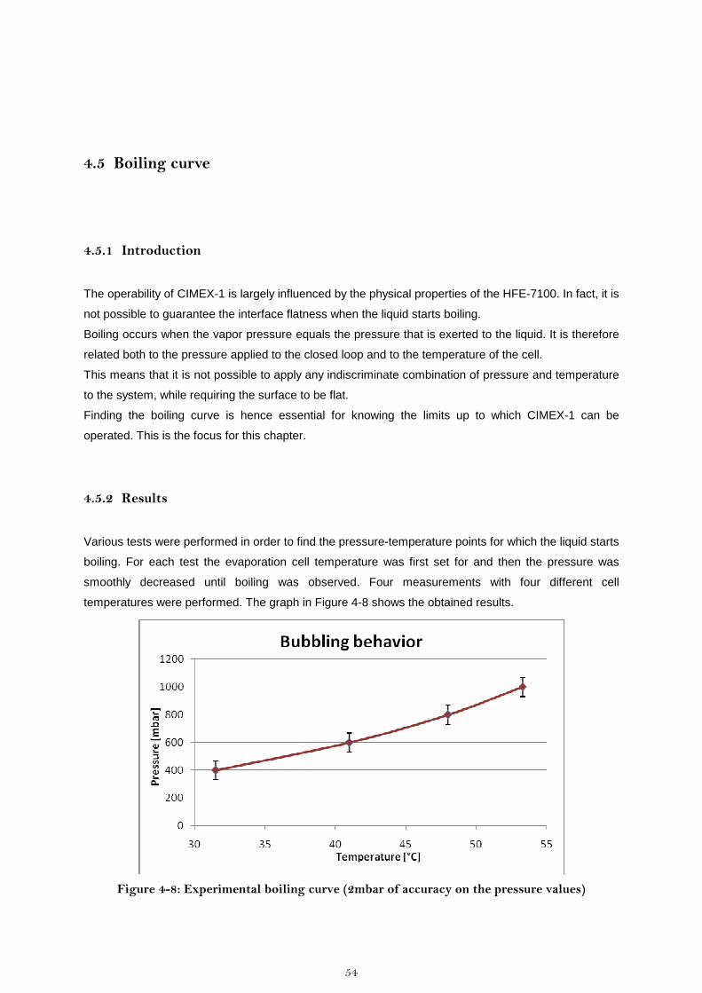
54

4.5 Boiling curve

4.5.1 Introduction

The operability of CIMEX-1 is largely influenced by the physical properties of the HFE-7100. In fact, it is

not possible to guarantee the interface flatness when the liquid starts boiling.

Boiling occurs when the vapor pressure equals the pressure that is exerted to the liquid. It is therefore

related both to the pressure applied to the closed loop and to the temperature of the cell.

This means that it is not possible to apply any indiscriminate combination of pressure and temperature

to the system, while requiring the surface to be flat.

Finding the boiling curve is hence essential for knowing the limits up to which CIMEX-1 can be

operated. This is the focus for this chapter.

4.5.2 Results

Various tests were performed in order to find the pressure-temperature points for which the liquid starts

boiling. For each test the evaporation cell temperature was first set for and then the pressure was

smoothly decreased until boiling was observed. Four measurements with four different cell

temperatures were performed. The graph in Figure 4-8 shows the obtained results.

Figure 4-8: Experimental boiling curve (2mbar of accuracy on the pressure values)

55

In the Figure 4-9 it is also possible see the differences between the obtained experimental curve and

the data from the pure HFE-7100 saturated case (from the literature).

Bubbling bahavior

Pure HFE case vs.Experiemtal case

0.000

0.100

0.200

0.300

0.400

0.500

0.600

0.700

0.800

0.900

1.000

1.100

-20 -10 0 10 20 30 40 50 60 70Temperature [°C]

Pre

ssu

re [

ba

r]

Pure HFE data

(Literature)

Experimental data

Figure 4-9: Bubbling curve vs. pure HFE boiling curve

From the graph in Figure 4-9 it is possible to see that the boiling occurs, for the same pressure values,

at lower temperatures than the pure HFE-7100 case. This behavior could be explained because of the

Nitrogen dissolved in the liquid. In fact, when the HFE-7100 is bubbling, the liquid also degasses. This

leads to different values than the ones obtained from the literature. Anyway, it has to be mentioned that

there are many other causes for which the experimental values differ to the ones from the literature.

One of them could be, for instance, the different roughness of the surfaces in contact with the liquid.

56

5 Measured raw data conversion and calculations

5.1 Introduction

The raw values from the MFM, the MFC and the GCS had to be converted, since the instruments were

calibrated for other operative conditions, more precisely:

• The GCS was calibrated for volumetric gas concentrations. Since the requirements impose

limitations on the mass concentration, a conversion from volumetric to mass concentration

was necessary.

• The MFM and the MFC were calibrated for a mixture of 95% of Nitrogen and 5% of Ethanol

vapor. A conversion is therefore needed to obtain the values for the measured mixture of

Nitrogen and HFE-7100 vapor. If the values were not changed, the post-processing analysis

would be completely wrong.

Moreover, the only available value for the outcome flow of the evaporation cell was the mass flow rate.

Knowing the concentration at both sides of the cell allows a better analysis of the performance of the

subsystem, especially of the CSS. Therefore, calculations must also be performed in order to obtain

the gas concentration after the evaporation cell.

This chapter focuses on the mentioned conversions and calculations. The outcome results will be used

for the post processing analysis of chapter 6.

57

5.2 Gas concentration conversion

5.2.1 Introduction and objectives

The GCS used for the test campaign was calibrated for volumetric concentrations. The project

requirement 3267 (see Annex 1:) states that the “CSS shall deliver at the outlet a gas phase composed

of at least 50% of gas” in which the composition is intended as a mass fraction. Therefore a conversion

method had to be found in order to obtain the mass concentration value.

A theoretical model based on the ideal gas theory was used to perform this transformation. The HFE-

vapor and Nitrogen will be considered as a mixture of ideal gases.

In the ideal gas theory there are two different models that can be used for mixtures of gases [1] :

• The Dalton model

• The Amagat model

The Amagat model was chosen for the calculation because the Dalton one was not suitable for the

current problem.

In fact the Dalton assumption states that:

”each mixture components behaves as an ideal gas as if it were alone at the temperature T

and the volume V of the mixture” [1]

Since the HFE volumetric concentration is defined as:

2NHFE

HFEVol VV

VC &&

&

+= (Eq. 2)

then the concentration would remain every time equal to 0,5 because, according to the Dalton model,

all the volumetric flow rates would have been considered equal:

mixtureNHFE VVV &&& ==2

(Eq. 3)

Therefore the Amagat model is considered for the conversion.

The model states that:

”each mixture components behaves as an ideal gas as if it existed alone at the temperature T

and the pressure p of the mixture” [1]

58

5.2.2 Analytical calculations

The partial volume that the component “i” of mixture occupies, according to the Amagat model, could

be calculated as follows:

p

TRnV i

i

⋅⋅= (Eq. 4)

Where ni is the number of moles of the component “i”, p is the pressure of the mixture, T is the mixture

temperature and R is the universal gas constant.´

The HFE volumetric concentration could therefore be expressed as following:

HFEMIXTURE

HFE

MIXTURE

HFE

MIXTURE

HFE

NHFE

HFEVol

yn

n

p

TRn

p

TRn

V

V

VV

VC ==

⋅⋅

⋅⋅

==+

=&

&

&

&

&

&

&&

&

2

(Eq. 5)

Where HFEy is the mole fraction of the HFE-7100.

The sum of the partial volumes has to be equal to the mixture volume, therefore:

⇒=+ MIXTURENHFE VVV &&&2

⇒=+ 12

MIXTURE

N

MIXTURE

HFE

V

V

V

V&

&

&

&

⇒=+ 12NHFE yy HFEN yy −= 1

2

volN Cy −=⇒ 12

(Eq. 6)

From the mass concentration definition it is possible to obtain the following relation:

HFE

NNHFE

HFEMass

m

mmm

mC

&

&&&

&

22 1

1

+=

+=

(Eq. 7)

The mass of the Nitrogen and the HFE-7100 can be calculated as following:

22222 NNNN MynMnmN

⋅⋅=⋅= &&& (Eq. 8)

HFEHFEHFEHFEHFE MynMnm ⋅⋅=⋅= &&& (Eq. 9)

M is the molecular weight of each component and “ n& ” is the mole flow rate of the Mixture.

Combing (Eq. 5), (Eq. 6), (Eq. 7), (Eq. 8) and (Eq. 9) it is finally possible to obtain the mass

concentration:

CCC

Vol

Vol

HFE

NNHFE

HFEMass

M

Mmm

m−

⋅+=

+=

11

1

22&&

&

(Eq. 10)

59

From this final equation it is possible to see that, according to the Amagat model, the mass

concentration of the mixture is function only of the volumetric concentration and of the molecular

weights of the Nitrogen and the HFE-7100. The temperature and the pressure of the mixture do not

affect the conversion.

Therefore the mass concentration can be easily calculated with this formula knowing only the gas

concentration sensor readout value.

5.2.3 Analysis of the results

Using Eq. 10 to perform the conversion, it is possible to obtain the graph shown in Fig.5-1, considering:

kmol

kgM N 01,28

2=

kmol

kgM HFE 250= (Eq. 11)

The HFE molecular weight value was found in the datasheet attached in Annex 6:

0

20

40

60

80

100

120

0 20 40 60 80 100 120Volumetric concentration [%]

Mas

s co

ncen

trat

ion

[%]

Figure 5-1: Conversion from volumetric to mass concentration. Values obtained theoretically using the Amagat model.

These results are very important because they show that the mass concentration becomes relatively

big even at small volumetric concentrations. In fact already at 10% of volumetric concentration the

mass fraction is 50%. This means that every test for which the volumetric concentration value was

above 10% it would be out of the mass fraction requirement 3267 of Annex 1:.

Mixture

Mix

ture

60

5.2.4 Validation of results using an experimental test

The curve reported in Figure 5-1 is purely theoretical and it is based on the preliminary assumptions:

the Amagat and the ideal gas models. In order to rely on this conversion method, an experimental

validation test was performed. The test setup consisted of a temperature controlled chamber which

mixed the measured amounts of Nitrogen and liquid HFE-7100, in order to deliver to the GCS (placed

after the mixer) a precise mass mixture quality. For each test, the volumetric concentration was

obtained from the sensor readout through Eq. 1, which was a result of a previous sensor calibration.

This value was then compared with the known mass concentration. Tests were performed at different

mixture pressures and temperatures.Figure 5-2 shows the validation results.

0

20

40

60

80

100

120

0 20 40 60 80 100 120

Volumetric concentration [%]

Mas

s co

ncen

tratio

n [%

]

Theoretical curve

Experimental curve

Figure 5-2: Conversion curve between the mass and the volumetric concentrations. Comparison between the experimental and the theoretical values.

During the tests, it was observed that both the temperature and the pressure did not affect the

conversion. This is an important result because it proves the accuracy of the theoretical relationship

(Eq.10), which is also not dependent on the pressure and temperature. Moreover, the points of the two

curves in Figure 5-2 are very close to each other and the trends are the same. However there are little

differences between the curves. The possible reasons are the presence of dissolved Nitrogen in the

HFE and the accuracy of the instruments used to feed the mixer. The maximum difference between

the experimental and theoretical values was 5%. It is therefore possible to say that the theoretical

method approximates the real values very well. The Amagat and the ideal gas assumptions are

therefore correct.

Mixture

Mix

ture

61

The following deductions can be made looking at the conversion relationship (Eq.10):

• The transformation curve gives higher mass concentrations in respect to the volumetric ones,

because the molar mass of the HFE is much more (almost 10 times) than the Nitrogen molar

mass.

• The only parameters that appear in the conversion are the volumetric concentration and the

molar weights of the mixture components.

5.3 Calibration of the MFM and MFC


The MFM and the MFC were calibrated for a mixture of 95% of Nitrogen and 5% of Ethanol. During the

test campaign, the meters measured a mixture of Nitrogen and HFE-7100. Therefore a conversion was

necessary in order to have correct results. The values were firstly converted to the fictitious case of

pure Nitrogen passing through the meters. This transformation was done by using a program from

Bronkhorst, named FLUIDAT[15], which provided a conversion factor of 1,048. Once the values were

converted to the pure Nitrogen case it was possible to perform the calculation to obtain the final value

for the mixture of HFE-7100 and Nitrogen. This chapter is about this calculation.

Even before computing the transformation, it could be easily noticed that, if the meters readouts were

converted as if the flow was pure Nitrogen, the error made would be relevant. In fact, considering that

the obtained mass concentration of the mixture was around 50% most of the time, and considering that

the molar mass of the HFE-7100 is almost 10 times the Nitrogen one, the real readout values are

expected to be quite different from the case with the Nitrogen calibration.

5.3.2 Calculations

The conversion factor cannot be calculated with FLUIDAT because the HFE-7100 fluid was not loaded

in the program archive. Moreover even if FLUIDAT had the HFE-7100 fluid properties, the

concentration of the HFE vapor would not be constant throughout all the tests range, and it would be

not convenient to perform the conversion for every one of the 55 measurements.

Therefore an alternative way was chosen by using a model proposed in the Bronkhorst` LOW-∆P-

METER instruction manual [6]. This choice was also suggested by a supplier expert.

The proposed formula in the manual for a gas mixture is:

62

n

n

mix C

V

C

V

C

V

C....

1

2

2

1

1 ++= (Eq. 12)

Where mixC is the conversion factor for the whole mixture, iC is the conversion factor for the “i”

component of the mixture and iV is the volumetric fraction of the “i” component in the mixture.

For the mixture used in CIMEX-1 (HFE vapor and-Nitrogen) Eq.12 becomes

HFE

HFE

N

N

mix C

V

C

V

C+=

2

21 (Eq. 13)

For the MFC HFEV is simply the volumetric concentration read by the GCS, namely volC , and

2NV = HFEV−1 , therefore volN CV −= 12

.

For the second conversion factor to be used for the MFM, positioned after the cell, another volumetric

concentration is needed for HFEV because the HFE vapor quantity increases, due to the evaporation in

the cell. Since is not possible to calculate this concentration, because it depends on the MFM readout

(see chapter 5.4, Eq.28), the same volumetric concentration, read by the GCS, is used also for the

MFM. Clearly, this is a source of error which has to be avoided in the future measurements, for

example implementing a second GCS after the cell or characterizing the liquid pump behavior.

Note: The following calculations are intended for the pure Nitrogen data (already converted from the

Nitrogen-Ethanol mixture calibrated data) to the desired HFE7100-Nitrogen data.

5.3.2.1 CN2 calculation

According to the Bronkhorst manual [6], the conversion factor for each component of the mixture has

to be calculated as following:

)2()2(

)1()1()21( ρ

ρ⋅⋅

=→p

p

c

cC (Eq. 14)

Where (1) is the gas to be calibrated and (2) is the gas to be measured. cp is the specific heat at

constant pressure and ρ is the gas density. The formula contains the thermal properties of the flow

since the working principle of the meters is based on the thermal bypass method. For further

information see section 2.3.5 and [6].

Note: according to the manual cp has to be taken at a temperature 50°C higher than t he one at

which the conversion factor is calculated. This recommendation will be applied for all the

following calculations, also for the CHFE calculations.

In the case of CN2 both the gas to be calibrated and the measured one are Nitrogen. Therefore the

conversion factor is 1.

12

=NC (Eq. 15)

63

5.3.2.2 CHFE calculation

In this case, according to Eq.14, the gas to be calibrated is HFE vapor and the gas to be measured is

Nitrogen. Therefore:

)()(

)()()2(

22

HFEHFEp

NNpHFEN c

cC

ρρ

⋅⋅

=→ (Eq. 16)

)( 2Npc is calculated from the relationship valid for ideal gases provided in table A-21 of Reference [1]:

)10226,010632,010324,210208,1675,3( 41239263)(

2

2TTTT

M

Rc

NNp ⋅⋅−⋅⋅−⋅⋅+⋅⋅−⋅= −−−− (Eq. 17)

Where R is the universal gas constant and 2NM is the Nitrogen molar mass, equal to

Kmol

Kg01,28

The Nitrogen density )( 2Nρ can be easily calculated using the ideal gas state equation:

TR

Mp NN ⋅

⋅= 2

2 )(ρ (Eq. 18)

Where p and T are the gas mixture pressure and temperature, respectively.

Also the HFE-7100 density )(HFEρ can be calculated using the ideal gas state equation:

TR

Mp HFEHFE ⋅

⋅=)(ρ (Eq. 19)

P and T are again the gas mixture pressure and temperature.

Unfortunately a formula like Eq.17 is not available for the HFE-7100 specific heat. Therefore this

quantity has to be calculated using the definition and the HFE-7100 vapor table that is possible to find

in Annex 4:.The specific heat at constant pressure is defined as:

pp T

hc

∂∂= (Eq. 20)

Where h is the mass specific enthalpy and T is the temperature

Since the vapor table provides all the enthalpy values for the correspondent temperatures, it is possible

to calculate the HFE-7100 specific heat by approximating the derivative in Eq.20 with the forward finite

difference as following:

p

HFEHFEpHFE T

ThTThpTc

∆−∆+= )()(

),( (Eq. 21)

With this approximation it was found that pHFEc varies from KKg

KJ

⋅94,0 to

KKg

KJ

⋅99,0 throughout

the full tested pressure range (400-1000 mbar) and the full tested temperature range (25-50°C). A

verification of these values was also performed in the pressure-enthalpy chart included in Annex 5:.

64

5.3.3 Results evaluation

The influence of the temperature and pressure on the conversion factor is negligible compared to the

influence of concentration. In fact, the graphs reported in Annex 2: show that the conversion factor

variations are only 1,5% throughout the temperature range, and only 1,4% throughout the pressure

range. The conversion factor was therefore correlated only with the volumetric concentration, being

sure that the final error will be negligeble.

Figure 5-3 presents the final results of the calculation, showing the conversion factor as a function of

the volumetric concentration, only.

Final results:Conversion factor vs. Volumetric concentration

0

0,2

0,4

0,6

0,8

1

1,2

0 20 40 60 80 100 120

Volumetric concentartion [%]

Con

vers

ion

fact

or

Figure 5-3: Conversion Factor for the MFM and the MFC

This data was finally used for the data conversion of the MFM and the MFC pure Nitrogen values.

For example 500 [mg/min] with the pure Nitrogen calibration, considering a volumetric concentration of

20 %, would correspond to:

tedHFEcalibracalibratedN min

mg19539,0

min

mg 500 rate flow HFE Real

2

=⋅= (Eq. 22)

5.3.4 Comments and recommendations

The concentration of the HFE is the main driver of the conversion factor calculation. Therefore, it is not

possible to adopt only one single conversion factor value for all of the test cases. Moreover, even if the

meters were calibrated for HFE-7100, with a specific concentration, a conversion factor would be still

needed because of the concentration variation during the tests. The conversion formula, according to

Mixture

N2

-> H

FE

65

Bronkhorst, is affected by an error which, in the worst case during the tests, was about 5%. This

inaccuracy cannot be avoided because it is prescribed in the formulas.

A more refined relationship for calculating the conversion factor should be found, taking into account

the temperature and the pressure influences. Moreover, the liquid pump behavior has to be

characterized to know exactly the volumetric concentration after the cell. With this value it will be

possible to calculate a more precise conversion factor for the MFM (see the comments after Eq.13(Eq.

13).

5.4 Calculation of the mass concentration after the cell


This chapter is meant to explain how the concentration at the cell outlet was calculated. This value is

important, because it allows a better assessment of the performances of the CSS (see chapter 6.4).

A mass balance will be applied to the evaporation cell.

5.4.2 Calculations

All the following calculations are based on the next scheme showed in Figure 5-4.

Figure 5-4: Scheme showing the cell inlets and outlet

At the inlet and at the outlet of the cell the mixture flow rate is:

INNHFEINMIXTUREIN mmm2

&&& += (Eq. 23)

OUTNHFEOUTMIXTUREOUT mmm2

&&& += (Eq. 24)

Mixture

outlet

Evaporation Cell

HFEINm&

INNm2

&

OUTNm2

&

Mixture

inlet

HFEOUTm&

Liquid inlet

66

Since the Nitrogen flow rate entering the cell is the same that leaves the cell (the liquid HFE contained

inside the liquid chamber is not supposed to absorb gas at steady state conditions):

INNm2

& =22 NOUTN mm && = (Eq. 25)

Form Eq.23 and from the definition of the mass concentration it is possible to calculate the Nitrogen

flow rate:

)1(2 massMIXTUREINHFEINMIXTUREINN Cmmmm −⋅=−= &&&& (Eq. 26)

Rearranging Eq.24 with Eq.26 it is possible to say that:

)1(2 massINMIXTUREINMIXTUREOUTNMIXTUREOUTHFEOUT Cmmmmm −⋅−=−= &&&&& (Eq. 27)

Considering the definition of mass concentration and Eq.27 it is finally possible to calculate the gas

concentration before the CSS:

MIXTUREOUT

massINMIXTUREIN

MIXTUREOUT

massINMIXTUREINMIXTUREOUT

MIXTUREOUT

HFEOUTmassOUT m

Cm

m

Cmm

m

mC

&

&

&

&&

&

& )1(1

)1( −⋅−=−⋅−==

(Eq. 28)

5.4.3 Comments and recommendations

massINC is calculated using Eq.10. Moreover, MIXTUREOUTm& is calculated from the MFM readout

converting the value to the HFE case. This calculation was performed considering the same volumetric

concentration as at the cell inlet (see the comments of Eq.13). Since the MFM converted value is an

approximation to the correct mass flow rate, also massOUTC , calculated from Eq.28, represents an

approximation to its real value.

More precise results will be available when the liquid pump behavior is characterized.

67

6 Analysis of the test data

6.1 Introduction

The aim of this section is to present the calculated results of the closed loop BB test campaign. The

data obtained directly from the instruments will be converted, according to the indications reported in

chapter 6.2. These conversions are important for a better assessment of the system performances.

Although the calculated results of CIMEX-1 are the main purpose for the real mission, they are not the

primary target for this BB test campaign. Anyway, they are the first results obtained with the HFE-7100;

the fluid replacing the previous Ethanol, and therefore they will be useful for the requirements

redefinition or for the first eventual design iteration of some components like the CSS.

The results are graphically reported in section 6.3 and 6.4. Tables containing all of the partial

calculation and additional information are reported in Annex 3:.

6.2 Used formulas

All the results that will be presented were obtained using the following calculations:

• Change from volumetric to mass gas concentration.

The theoretical background and the performed calculation are presented in chapter 5.2.

• Conversion from the “apparent” volumetric flow unit readout of the Bronkhorst meters to the

mass flow unit.

The instruments readouts are expressed in units of Volume, ml/min, but they are normalized to

a constant temperature and pressure: 0°C and 1,013b ar. This means that, although the

readouts are in units of volume, the measurement is a mass flow.

68

To convert the result in units of mass the Nitrogen density at 0°C and 1,013bar was calculated.

Its value was 1,2504mg/ml and it was used for both the MFM and the MFC.

min08,2502504,1

min200

min200 :Example

mg

ml

mgmlml

nn

=⋅= Eq. 29

Note: in order to highlight that the MFM readout is a mass flow, even if it expressed in

unit of volume, a subscript n (meaning “normalized”) will be used.

• Conversion from the N2+Ethanol calibration to the pure Nitrogen calibration.

This calculation was performed for both meters. The used conversion factor was 1,048, and it

was provided by the supplier.

22 min524048,1

min500 :Example

pureNEthanolN

mlmg =⋅+

Eq. 30

• Conversion from the pure N2 calibration to the HFE calibration.

This calculation was performed for both the MFM and the MFC using the conversion factor

calculated in chapter 5.3. The factor depends on the volumetric concentration and it is

therefore different for each test case.

Example of conversion: 500 [mg/min] with the pure Nitrogen calibration, considering a

volumetric concentration of 20 %, would correspond to:

tedHFEcalibracalibratedN min

mg19539,0

min

mg 500 rate flow HFE Real

2

=⋅=

Eq. 31

See chapters 5.3.3 and 5.3.4 and check the comments of this conversion method

• Calculation of the mixture volumetric flow rate.

This calculation was performed only for the MFC using the following mixture density:

TR

Mp MixtureMixture ⋅

⋅=)(ρ Eq. 32

T is the temperature of the mixture which is equal to the ambient temperature (26°C) since the

line was not thermally isolated. P is the test pressure. MixtureM is the molar mass of the

mixture and it is equal to:

222 )1( NvolHFEvolNNHFEHFEMixture MCMCMyMyM ⋅−+⋅=⋅+⋅= Eq. 33

Finally the volumetric flow rate was calculated from the mass flow rate by using:

)(Mixture

HFEmixture

HFEmixture

mV

ρ&

& =

Eq. 34

69

• Calculation of the gas concentration after the cell.

Eq.28 in chapter 5.4 was used for this calculation.

• Gas concentration percentage reduced by the CSS (or CSS efficiency):

This parameter was considered for a better assessment of the CSS performance because it is

independent on the flow rate. In fact, the efficiency is the ratio between the mass concentration

reduced by CSS and the mass concentration that enters in the condenser.

The definition of the efficiency is the following:

massIN

massOUTmassIN

C

CC −=η

Eq. 35

• Evaporating HFE flow rate.

This calculation is performed by subtracting the MFC mass flow to the MFM mass flow:

tedHFEcalibratedHFEcalibra MFCMFM rate flow HFE gEvaporatin −=

Eq. 36

6.3 Cell behavior

The calculated results of the cell are about the evaporation rate as a function of the main parameters:

the cell temperature, the gas loop pressure and the mixture flow rate. Figure 6-1 and Figure 6-2

summarize the results of the tests. In the graph below, it is possible to see that as the volumetric flow

rate increases, the evaporating liquid flow rate also increases. Moreover, the lower the pressure, the

higher the evaporation rate.

0

10

20

30

40

50

60

70

80

90

100

0 100 200 300 400 500 600 700 800 900 1000

Mixture volumetric flow rate before the cell [ml/min]

Eva

pora

ting

liqui

d flo

w r

ate

[mg/

min

]

p=1000mbar

p=500mbar

p=400mbar

Figure 6-1: Evaporating fluid flow rate vs. mixture volumetric flow rate @ T=25°C

70

The following second graph shows that, the higher the temperature, the higher the evaporation rate,

and the higher the volumetric flow rate, the higher the evaporation rate.

0

0

10

20

30

40

50

60

70

80

90

100

0 50 100 150 200 250 300 350 400 450 500

Mixture volumetric flow rate before the cell [ml/min]

Eva

pora

ting

liqu

id fl

ow ra

te [m

g/m

in]

T=25°C

T=30°C

T=40°C

Figure 6-2: Evaporating fluid flow rate vs. mixture volumetric flow rate @ p=1000 mbar

6.4 CSS behavior

The CSS behavior will be assessed using the efficiency defined in section 6.2. Next graph summarizes

the results; comments are provided in the next page.

0

5

10

15

20

25

30

35

0 50 100 150 200 250 300 350 400 450

Volumetric flow rate before the cell [ml/min]

Cel

l effi

cien

cy [%

]

Temperature=30°C

Temperature=40°C

Figure 6-3: CSS efficiency vs. cell temperature @ 1000 mbar

71

The information contained in the previous graph can be summarized as following:

• The higher the cell temperature, the lower the cell efficiency. This could be explained because

of the higher evaporation rate at higher temperatures (see the graphs in section 6.3). With a

higher evaporation rate, the cell efficiency decreases.

• The higher the volumetric flow rate, the lower the efficiency. This could be explained because

at high volumetric flow rates, the evaporation rate increases (see the graphs in section 6.3)

and consequently the CSS efficiency decreases.

Another important result can be easily verified by looking at Table 9 in Annex 3:. The mass

concentration after the CSS exceeds the 50% value for about half of the performed tests. This is very

important for CIMEX-1, since the requirements state that the concentration should not exceed this

value. However, it is important to say that the CSS was designed for Ethanol and not for HFE-7100.

For this reason, the requirements are not satisfied. A requirements redefinition or a new CSS design is

therefore necessary. Further considerations about the implication of this behavior are reported in

chapter 7.

6.5 Comparison with the Ethanol case

In 2008, VERHAERT space [17] tested the CSS with Ethanol. The aim of this section is to compare the

results obtained with Ethanol to the ones obtained during the test campaign with HFE-7100.

The graph in Figure 6-4 shows the results obtained with the Ethanol mixture from the VERHAERT test.

Figure 6-4: CSS behavior with Ethanol according to reference [4] (from VERHAERT SPACE)

72

For the values shown in Figure 6-4, the CSS efficiency is calculated according to Eq.35 in section 6.2

and the plot in Figure 6-5 is then obtained. From this plot it is possible to see that the CSS efficiency

increases as the concentration of the entering gas increases.

0

10

20

30

40

50

60

70

80

90

0 5 10 15 20 25 30 35 40

Gasconcentration before the CSS [%mass]

CS

S e

ffic

ienc

y [%

]

Figure 6-5: CSS efficiency vs. gas concentration entering the CSS using the VERHAERT SPACE test report data. Ethanol case

These results can be compared with the HFE-7100 data which are reported in Figure 6-6

As it is possible to see, the CSS behavior is the same: the efficiency increases as the inlet gas

concentration increases.

0

5

10

15

20

25

30

35

45 47 49 51 53 55 57 59 61

Gas concentration before the CSS [%mass]

Cel

l eff

icie

ncy

[%]

Figure 6-6: CSS efficiency vs. HFE-7100 gas concentration entering the CSS. (1000mbar, condenser @-20°C)

However, the cell efficiency using HFE-7100 mixture is much less than the case with Ethanol mixture.

73

A possible reason comes from the conversion factor used to obtain the mass concentration from the

volumetric concentration. In fact, this transformation is affected by the molar weight ratio between the

Nitrogen and the vapor, according to Eq.10 of section 5.2. The graph in Figure 6-7 shows the different

relationships between the mass and the volumetric concentration for the Ethanol case and the HFE

case. For the same value of volumetric concentration, the corresponding mass concentration would be

less in the case of Ethanol because its molar mass is only 46,07g/mol, while the HFE-7100 is

250g/mol. Therefore, the CSS would have more mass to condense in the case with HFE-7100 and the

efficiency would consequently decrease.

0

20

40

60

80

100

120

0 20 40 60 80 100 120

Volumetric concentration [%]

Mas

s co

ncen

tratio

n [%

]

N2+HFE-7100 vapor

N2+ethanol vapor

Figure 6-7: Relationship between the mass and volumetric concentration HFE-7100 vs. Ethanol

6.6 Comments

The obtained results make physical sense but they cannot be considered valid for scientific use, since

some instruments were not precise enough for scientific purposes. However, they are suitable for

engineering purposes like redesigning components or proposing new requirements (as it will be done

in the next chapter).

For a correct evaluation of the results, it is important to note that the same conversion factor was used

both for the MFM and for the MFC. This assumption caused errors in the performed calculations of this

chapter since:

• The same volumetric concentration which was used for the MFC conversion factor was also

considered for the MFM conversion factor. Obviously the two concentrations are different due

74

to the evaporation taking place in the cell. This choice was made, since it is not possible to

calculate the exact volumetric concentration after the cell with this test setup, because the

respective mass concentration (from which it is possible to calculate the volumetric

concentration through Eq.10), depends on the MFM readout, which in turn depends on the

volumetric concentration. An extra input parameter is therefore missing. When the flow rate

delivered by the liquid pump will be known (by characterizing the pump behavior), the mass

concentration can be correctly calculated at the cell outlet. Therefore, after converting the

mass concentration to the respective volumetric concentration (by inverting Eq.10 in section

5.2), it will be possible to correctly calibrate the MFM using the formulas presented in section

5.3.

• The MFM and MFC pressures and temperatures were considered equal because of the small

influence of these parameters on the conversion.

The CSS was not able to deliver less than 50% of vapor quality for all the conditions. On the contrary

the tests performed by VERHAERT Space with Ethanol, instead of HFE-7100, were all within the

requirement range. As it was pointed out in section 6.5 the reason for this different behavior is the

different molecular weights of the liquids.

The most important remark of this chapter is the discovery that the mass concentration requirement

was not satisfied. Therefore, a solution has to be found in order for the project to continue. Since much

effort has been made for designing, building and testing the components, it was decided to change the

requirements instead of performing a new design (in particular for the CSS). Chapter 7 will present a

requirement redefinition which will be proposed and agreed with the European Space Agency and the

teams of scientists.

75

7 System evaluation and requirements redefinition

7.1 Introduction

In this last chapter, the results obtained during the test campaign were summarized and an evaluation

of the System Operability/Stability with HFE-7100 was performed. The aim of the following sections is

to assess the System behavior and to obtain suitable parameter ranges for the system with HFE-7100.

7.2 System stability and operability evaluation

The start-up of the system was demonstrated to be functional and CIMEX-1 closed loop was stable

with the HFE-7100. The surface flatness and the meniscus stability were achieved by manual hand

control of the injection rate (the control frequency was estimated to be about 1Hz). At lower pressures

and high evaporation rates, the manual control becomes more challenging but it is still achievable. The

system stability can be considered achieved. The surface flatness control by PID control loop will be

implemented in the future with sampling rates higher than 1Hz. It is assumed to be very feasible to

automatically control all required parameter ranges.

The system evaporation across the loop was controlled. It was demonstrated that it is possible to

recover the system to the initial operational conditions without opening the loop after chaotic conditions

(e.g. boiling of HFE-7100). Moreover, if the spilling of liquid over the micro-groove was enforced, the

system recovery was demonstrated to be feasible within 1-3mins as well as a restart of the flatness

control.

The operability of the system and the system stability were achieved during the closed loop test

campaign. From this point of view, the BB tests were successful.

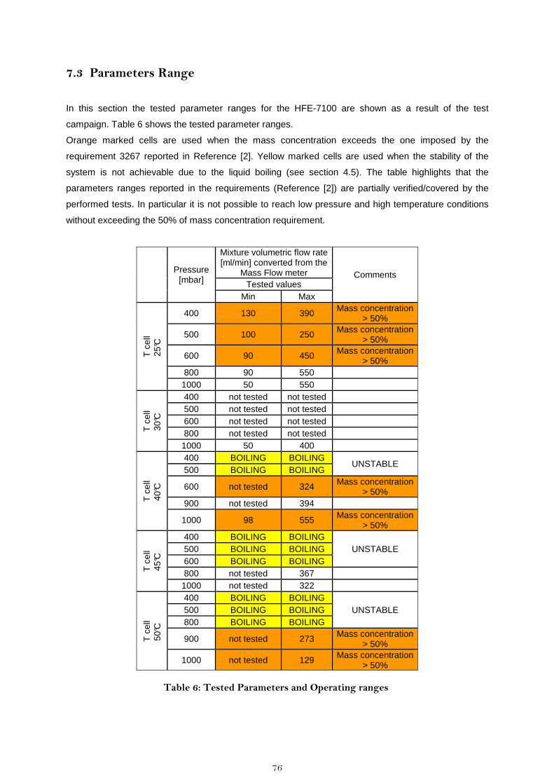
76

7.3 Parameters Range

In this section the tested parameter ranges for the HFE-7100 are shown as a result of the test

campaign. Table 6 shows the tested parameter ranges.

Orange marked cells are used when the mass concentration exceeds the one imposed by the

requirement 3267 reported in Reference [2]. Yellow marked cells are used when the stability of the

system is not achievable due to the liquid boiling (see section 4.5). The table highlights that the

parameters ranges reported in the requirements (Reference [2]) are partially verified/covered by the

performed tests. In particular it is not possible to reach low pressure and high temperature conditions

without exceeding the 50% of mass concentration requirement.

Pressure [mbar]

Mixture volumetric flow rate [ml/min] converted from the

Mass Flow meter Comments

Tested values Min Max

T c

ell

25°C

400 130 390 Mass concentration > 50%



800 90 550 1000 50 550

T c

ell

30°C

400 not tested not tested 500 not tested not tested 600 not tested not tested 800 not tested not tested

1000 50 400

T c

ell

40°C

400 BOILING BOILING UNSTABLE

500 BOILING BOILING

600 not tested 324 Mass concentration > 50%

900 not tested 394


T c

ell

45°C


500 BOILING BOILING 600 BOILING BOILING 800 not tested 367

1000 not tested 322

T c

ell

50

°C


500 BOILING BOILING 800 BOILING BOILING



Table 6: Tested Parameters and Operating ranges

77

7.4 New proposed requirements

As a result of the previous findings, the following new requirements are proposed for CIMEX-1 in order

to keep the already existing design and, when possible, components.

Spec ID*

Chapter*

Requirement Current values New proposed values

3267 4.3.14.1 The CSS shall deliver at outlet a gas

phase composed of at least 50% of gas. 95% is considered as a target.

50% of Nitrogen (in

Mass)

Up to 20% of Nitrogen (in Mass), target 95%.

Or

Up to 60% of Nitrogen (in volume) target 95%

(*1)

3205 4.3.7.1.1 The temperature setting range shall

be 10°C up to 60°C. 10°C to 60°C 10°C to 50°C (*2)

3193 4.3.5.3 The gas flow rate shall be measurable

in a range from 10 to max 1000 ml/min.

10-1000 ml/min

10-1000 ml/min (*3)

3197 4.3.6.1 The set pressure shall be adjustable in

a pressure range from 400 mbar to 1000 mbar.

400-1000 mbar Variable from 500 to1000

mbar according to the boiling curve (*4)

*Chapter and ID are intended for Reference [2]

Table 7: New proposed requirements

Remarks:

• (*1) The molar mass of HFE-7100 is much higher than the Ethanol, therefore the mass

concentration while entering the CSS is much higher with the same volumetric concentration

(see Figure 6-7) and as a consequence it is better to re-define the requirement to a volumetric

concentration. It has been observed that for low evaporation rates, the gas concentration is

very low (e.g. 6-7%vol).

• (*2) The hardware is designed to support a temperature up to 60°C. The upper limit of the

temperature range is due to the bubbling/degassing of the HFE-7100 at 1bar, which is the

maximum experiment pressure (see Figure 4-9).

Nevertheless, there will be combinations which are not possible due to bubbling as described

in the same figure (e.g. high temperature and low pressure).

• (*3) The Bronkhorst devices will be calibrated to pure gas (Nitrogen case), since the real

volumetric flow is dependent on the gas concentration (also temp and pressure). This can

mean in some cases, a “real” flow (of Nitrogen + HFE-7100), below 500ml/min (even if

1000ml/min where commanded, see Table 9). This occurs in cases when the HFE-7100

concentration is high in the entrance of the cell.

This means post-processing of the volumetric flow will have to be considered by the scientific

team during results evaluation.

• (*4) Pressure ranges are fine, with the remark that it is not possible to have all combinations

with the temperatures (see Figure 4-9).

78

8 Conclusions

This project demonstrated, for the first time, that CIMEX-1 is able to work in a complete closed loop

with the new selected HFE-7100 liquid. This is an important step, since it is mandatory for the mission

development to be continued. The system worked fine with challenging conditions (i.e. high cell

temperatures and low pressures), and manual controlling was possible for all of the tests. The system

recovered successfully after chaotic conditions, without the need to open the circuit.

The Bronkhorst meter/controller worked fine during all of the test campaign. Since the instruments

were calibrated for another mixture, the measured values were converted using the indications

provided by the supplier. It was discovered that this conversion was mostly affected by the mixture

quality. Therefore, a conversion would be necessary even in the case that if the meters were calibrated

for a mixture of and Nitrogen and HFE-7100 with a certain, but fixed concentration. The conversion

formula was affected by an error of 5%. A more precise calculation method should be found in the

future for better results. Moreover, for the same reason, the conversion factor variations with the

mixture temperature and pressure should be taken into account.

The GCS worked fine, and the jumps problem due to the buffer overflow was solved by implementing

the Java program. The program has to be improved since it experienced a wrong behavior when liquid

HFE-7100 wetted the instrument. The conversion from volumetric to mass concentration was

successfully performed and the theoretical assumptions were validated by performing experimental

tests. This conversion also explained why the system behavior with HFE-7100 is different than with

Ethanol (i.e. because of the bigger molecular weight). However, a dedicated sensor calibration for

mass concentrations is needed for better results.

The metallic foil with the anti-wetting groove worked effectively, demonstrating that is possible to keep

the liquid level above the foil surface and to reach the liquid interface stability.

A proposal for new requirements was given in order to maintain wider parameter ranges (regarding

pressures and flow rates). Another choice could be a re-design of some components (e.g. the CSS)

and the results of this BB could be used for the first design iteration. The science teams, as well as

ESA, will verify which of these options is more suitable for the scientific purposes.

It is possible to conclude that CIMEX-1 Closed Loop BB was a success.

79

Bibliography

[1] M.J. Moran, H.N. Shapiro, Fundamentals of Engineering Thermodynamics, John Wiley &

Sons, FIFTH EDITION 2006

[2] CIMEX-1 System Specification, F6-SP-AST-0002 issue 06, EADS Astrium document, 2008

[3] FSL EC B1 CIMEX-1 Design report incl. Functional and Performance analysis report, F6-RP-

AST-0380 issue 02, EADS Astrium document, 2008,

[4] CIMEX FCA Bredboard-Test Procedure-Report, F6-RP-VDD-0064 issue C, VERHAERT

Space document, 2008

[5] Requirements specifications, CIMEX1-ESA-ERD-001

[6] Instruction manual: Mass Flow/Pressure meters and controllers for gases and liquids,

Bronkhorst, doc. N.9.17.001N, 27-06-2011

[7] C. S. Iorio, Experimental and numerical study of the coupling between evaporation and

thermocapillarity Preparation of the CIMEX-1 Experiment, PhD thesis, Université Libre de

Bruxelles, Septermber 2006.

[8] L.Ganuza, Devolopment Tests for an Evaporation Experiment in Microgravity, Master thesis,

October 2010, ISAE University

[9] J. C. Legros, Report on CIMEX-An ESA-Sponsored Reserch Program, September 2007

[10] J.C. Legros, P. Colinet, L.Joannes, P.Stephan, G. Bekaert, G. Lebon, P.Cerisier, A.Delil, M.

Bestehorn; Convection and Interfacial Mass Exchange CIMEX

[11] Bronkhorst website, www.bronkhorst.com

[12] ESA website, www.esa.int/esaHS/ESAAYI0VMOC_iss_0.html

[13] CIMEX FCA Bredboard-Test Procedure-Report, F6-RP-VDD-0064 issue C, VERHAERT

Space document, 2008

[14] CIMEX-F6 FCA & Optics Design Report, F6-RP-VDD-0018 issue D, VERHAERT Space

document, November 21st 2008

[15] FLUIDAT®, program for calculation mixture and fluid properties, Bronkhorst Company

[16] Lab VIEW®, program for data acquisition/conditioning and for automatic controlling

http://sine.ni.com/np/app/flex/p/ap/global/lang/en/pg/1/docid/nav-77/

[17] VERHAERT space (now QinetiQ Space nv), company involved in the CIMEX-1 development,

http://www2.qinetiq.com/home_qinetiq_space_nv.html

80

Annex 1: Requirements

Table 8: CIMEX-1 Requirements that were considered for the closed loop test campaign (information taken from [2])

Spec ID Chapter Title Requirement Text

3138 4.2.2.4.1 Gas Flow Control The gas system including pump shall allow to re-inject a defined gas flow rate at defined constant pressure into the fluid cell throughout the full fluid system pressure range.

3185 4.3.3.3. Liquid Flow Rate:

Pressure Range The liquid flow rate shall be adjustable and measurable in the presences of at a system-pressure from 400 mbar to 1000 mbar.

3187 4.3.4.1 Range of Depth

The liquid depth shall be adjustable in the range from 1mm to 10 mm for 3D fluid cell with a minimum of 5 steps - 1 mm - 2 mm - 3 mm - 5 mm - 10 mm Note: Fall back option: reduction of liquid layer depth 1 to 5 mm (only 4 depths would be tested).

3191 4.3.5.1 Gas Flow Control: Adjustable Range

The gas flow rate shall be adjustable in a range from 10 to max 1000 ml/min throughout the full pressure range of the gas from 400 to 1000 mbar.

3192 4.3.5.2 Gas Flow Control:

Accuracy The gas flow rate shall be controlled with an accuracy of 2% of the maximum flow rate.

3193 4.3.5.3 Gas Flow Rate:

Measurement Range The gas flow rate shall be measurable in a range from 10 to max 1000 ml/min.

3194 4.3.5.4 Gas Flow Rate: Measurement

Accuracy

The gas flow rate shall be measurable with an accuracy of 2% of the maximum measurement range.

3195 4.3.5.5 Gas Flow Rate: Calibration Data

Appropriate calibrations data with the given accuracy shall be supplied for the selected gas and gas mixture (with evaporated liquid).

3196 4.3.6 Pressure Control The FCA shall provide pressure control of the gas and liquid system in order to maintain a constant pressure in the cell at the pressure set value while other parameters like gas flow rate, liquid depth and separation percentage are adjusted.

3197 4.3.6.1 Pressure Control

Range The set pressure shall be adjustable in a pressure range from 400 mbar to 1000 mbar.

3198 4.3.6.2 Pressure Control

Accuracy The pressure control accuracy shall be better than 2% of the maximum measurement range.

3199 4.3.6.3 Pressure

Measurement Range The pressure shall be measurable in a pressure range from 100 mbar to 1400 mbar.

3200 4.3.6.4 Pressure

Measurement Accuracy

The pressure shall be measurable with and accuracy of 2% of the maximum pressure value.

3204 4.3.7.1 Temperature Control

of Cell The fluid cell temperature shall be regulated to a stable level by closed loop control.

3205 4.3.7.1.1 Temperature Range The temperature setting range shall be 10°C up to 60°C.

3207 4.3.7.1.3 Temperature

Absolute Accuracy The absolute temperature measurement accuracy within the fluid cell shall be better than ± 0.25°C.

3208 4.3.7.1.5 Temperature

Stability in Time The relative temperature control stability in time in the fluid cell shall be better than ± 0.05 K in one hour.

3211 4.3.7.1.8 Condensation

Prevention

The cell shall be maintained at a temperature higher than the saturation temperature corresponding to the vapour pressure to prevent condensation on the transparent walls.

81

Spec ID Chapter Title Requirement Text

3229 4.3.7.4 Injected Liquid Temperature

The liquid reaching the cell shall be at the same temperature as the liquid temperature within the cell within a range of ± 0.05 K, to prevent that the liquid situation within the cell will be perturbed. Note: This can be achieved by controlling the liquid injection path (i.e. reservoir and pipe).

3267 4.3.14.1 Condenser/Separator

Performance The CSS shall deliver at outlet a gas phase composed of at least 50% of gas. 95% is considered as a target.

3268 4.3.14.2 Condenser/Separator

Accuracy The CSS shall allow to control the percentage of residual vapour in the gas phase to a desired value with an accuracy of 2% FS (mass ratio).

3269 4.3.14.3 Temperature Control The condenser temperature shall be controlled by a feedback from the gas composition sensor (para. 4.3.13). This control shall be completely automatic and telecommanded.

3511 4.3.7.2 Temperature of Gas The gas temperature shall be regulated to the same temperature as the cell (± 0.5°C).

3512 4.3.7.2.1 Temperature Range The gas temperature range shall be 10°C up to 60°C.

3514 4.3.7.2.3 Absolute Accuracy The absolute gas temperature measurement of the gas shall be better than ± 0.25 K.

3784 4.1.8.1.1 Number of Liquid

Depths

The FCA shall be capable such that 5 different depths can be adjusted and measured. Note: CIMEX FCA verification by Review only.

3835 4.3.14.6 Worst Operating

Conditions Condenser shall be dimensioned to cope with worst operating conditions, i.e. low pressures (400 mbar) and high flowrates (1000ml/min).

3875 4.2.3.7.3 Material Fluid Compatibility

Surface materials, treatments and coatings shall demonstrate long term stability in material compatibility test against the selected liquids.

82

Annex 2: Conversion factor variation

In these two graphs it is possible to appreciate the small variations of the conversion factor for the

MFC/MFC throughout all the pressure and temperature range. For more information, see the

calculations performed in chapter 5.3.

Conversion factor vs. Temperature @400mbar Maximum variation: 1,5%

0,207

0,210

0,213

0,216

0,219

348 353 358 363 368

Temperature [K]

Mix

ture

con

vers

ion

fact

or

Conversion factor vs. pressure at 50°CMaximum variation: 1,4%

0,201

0,204

0,207

0,210

0,213

300 450 600 750 900 1050

Pressure [mbar]

Mix

ture

con

vers

ion

fact

or

83

Annex 3: Data elaboration tables

Table 9: Data elaboration table

Gas properties before the cell Gas properties after the cell

Tes

t N

r.

Gas pressure

Cell Temp

Gas mass Flow rate (before

cell)

N2+Ethanol Calibrated

Gas pressure controller

Cell Temp


cell)


Gas Flow rate (before cell)

N2 Calibrated

Conversion factor

N2->(HFE+N2)mix


HFE-7100 Calibrated

Mixture density

(before cell)

Gas Volumetric flow rate

(before cell) [ml/min]

Gas mass Flow rate (after cell)





N2 Calibrated

Gas Flow rate (after cell)

HFE-7100 Calibrated

Evaporating liquid flow rate

Gas Conc before the cell

Gas Conc (%Vol)

Gas Conc after the cell

Percentage of the Gas

Concentration reduced by the

CSS

[mbar] [°C] [ml/min] n [mbar] [°C] [mg/min] [mg/min] [] [mg/min] [mg/ml] [ml/min] [ml/min] [mg/min] [mg/min] [mg/min] mg/min] [%Mass] [%Vol] [%Mass] [%]

1 1000 25 100 1 26 125 131 0,658 86 1,8 49 142 178 186 122 36 40,1 7 57,8 30,6

2 1000 25 400 1,06 26 500 524 0,694 364 1,7 218 505 631 662 459 96 36,2 6 49,5 26,8

3 1000 25 800 1,06 26 1000 1048 0,694 728 1,7 437 877 1097 1149 798 70 36,2 6 41,8 13,4

4 1000 25 1000 1,07 26 1250 1310 0,694 910 1,7 546 1078 1348 1413 981 71 36,2 6 40,8 11,3

5 1000 25 900 1,07 26 1125 1179 0,694 819 1,7 491 995 1244 1304 905 86 36,2 6 42,3 14,4

6 1000 25 1000 1,07 26 1250 1310 0,625 819 1,8 444 1075 1344 1409 880 61 43,6 8 47,6 8,3

7 1000 25 400 1,07 26 498 522 0,625 326 1,8 177 470 588 616 385 59 43,6 8 52,3 16,5

9 1000 25 800 1,12 25,9 999 1047 0,694 727 1,7 436 870 1088 1140 791 65 36,2 6 41,4 12,6

10 1000 30 100 1,05 29,9 124 130 0,658 85 1,8 49 150 188 197 129 44 40,1 7 60,5 33,7

11 1000 30 400 1,03 29,9 500 524 0,658 345 1,8 196 480 600 629 414 69 40,1 7 50,1 19,9

12 1000 30 800 1,01 29,9 1002 1050 0,658 691 1,8 393 880 1100 1153 759 68 40,1 7 45,5 11,8

13 1000 30 900 1 29,9 1125 1179 0,625 737 1,8 399 1000 1250 1310 819 82 43,6 8 49,3 11,4

14 1000 40 100 1,08 40,2 125 131 0,394 52 2,8 18 190 238 249 98 46 67,6 19 83,0 18,5

15 1000 40 400 1,04 40,1 501 525 0,408 214 2,7 78 535 669 701 286 72 66,1 18 74,6 11,4

16 1000 40 100 1,06 40,2 125 131 0,394 52 2,8 18 190 238 249 98 46 67,6 19 83,0 18,5

17 1000 40 400 1 40,8 563 590 0,368 217 3,0 72 590 738 773 285 68 70,3 21 77,3 9,1

18 1000 40 900 0,99 40,6 1127 1181 0,394 465 2,8 165 1075 1344 1409 555 90 67,6 19 72,8 7,2

19 1000 50 800 0,97 49,9 1000 1048 0,368 386 3,0 129 983 1229 1288 474 88 70,3 21 75,8 7,3

84


Tes

t N

r.

Gas pressure

Cell Temp


cell)



Cell Temp


cell)



N2 Calibrated

Conversion factor

N2->(HFE+N2)mix


HFE-7100 Calibrated

Mixture density

(before cell)



Gas mass Flow rate (after

cell)



cell)



cell)

N2 Calibrated


HFE-7100 Calibrated



Gas Conc (%Vol)



Concentration reduced by the

CSS

[mbar] [°C] [ml/min]

n [mbar] [°C] [mg/min] [mg/min] [] [mg/min] [mg/ml] [ml/min] [ml/min] [mg/min] [mg/min] [mg/min] [mg/min] [%Mass] [%Vol] [%Mass] [%]

20 1000 50 400 0,97 50,5 500 524 0,357 187 3,1 60 590 738 773 276 89 71,5 22 80,7 11,4

21 1000 25 1000 1,03 25,5 1248 1308 0,625 817 1,8 443 1083 1354 1419 886 70 43,6 8 48,0 9,2

21 800 25 800 0,8 26,2 1007 1055 0,694 732 1,3 549 1135 1419 1487 1032 300 36,2 6 54,8 33,9

23 500 25 1000 0,52 26,2 1250 1310 0,625 819 0,9 888 1112 1390 1457 910 92 43,6 8 49,3 11,5

24 600 40 800 0,63 39,6 1003 1051 0,456 479 1,5 324 1020 1275 1337 610 130 61,1 15 69,4 12,0

25 600 45 800 0,65 40,6 1000 1048 0,495 519 1,4 377 1070 1338 1402 694 175 57,1 13 67,9 16,0

26 800 45 800 0,78 45,3 1000 1048 0,517 542 1,8 308 1116 1395 1462 756 214 54,8 12 67,6 18,9

28 900 50 800 0,9 48,5 1000 1048 0,517 542 2,0 273 1002 1253 1313 678 137 54,8 12 63,9 14,2

29 900 25 800 0,95 24,5 1000 1048 0,566 593 1,8 326 877 1097 1149 651 57 49,7 10 54,1 8,2

30 800 25 800 0,8 24,6 1000 1048 0,540 566 1,7 335 892 1115 1169 632 65 52,4 11 57,3 8,6

31 800 25 400 0,8 24,7 500 524 0,540 283 1,7 168 474 593 621 336 52 52,4 11 59,8 12,4

32 800 25 200 0,8 24,7 250 262 0,625 164 1,5 111 265 331 347 217 53 43,6 8 57,4 24,1

33 600 25 800 0,6 24,8 1000 1048 0,540 566 1,3 447 896 1120 1174 634 68 52,4 11 57,5 8,9

34 600 25 400 0,6 25 500 524 0,540 283 1,3 223 480 600 629 340 57 52,4 11 60,3 13,2

35 600 25 200 0,6 25 250 262 0,475 124 1,4 87 260 325 341 162 37 59,2 14 68,6 13,7

36 500 25 400 0,5 25,1 500 52 4 0,517 271 1,1 246 480 600 629 325 54 54,8 12 62,3 12,1

37 1000 25 200 1,02 25,2 249 261 0,658 172 1,8 98 253 316 332 218 47 40,1 7 52,9 24,2

38 800 25 200 0,81 25,3 250 262 0,566 148 1,6 92 250 313 328 185 37 49,7 10 59,8 16,8

39 800 25 800 0,83 25,3 1000 1048 0,625 655 1,5 444 870 1088 1140 712 57 43,6 8 48,2 9,4

40 900 40 800 0,93 39,3 1000 1048 0,625 655 1,7 394 992 1241 1300 812 157 43,6 8 54,5 20,0

85


Tes

t N

r.

Gas pressure

Cell Temp

Gas mass Flow rate (before cell)



Cell Temp

Gas mass Flow rate (before cell)



N2 Calibrated

Conversion factor

N2->(HFE+N2)mix


HFE-7100 Calibrated

Mixture density

(before cell)








N2 Calibrated


HFE-7100 Calibrated



Gas Conc (%Vol)



Concentration reduced by the CSS

[mbar] [°C] [ml/min]

n [mbar] [°C] [mg/min] [mg/min] [] [mg/min] [mg/ml] [ml/min] [ml/min] [mg/min] [mg/min] [mg/min] [mg/min] [%Mass] [%Vol] [%Mass] [%]

41 800 45 800 0,8 45,4 1000 1048 0,566 593 1,6 367 1050 1313 1376 779 185 49,7 10 61,7 19,4

42 1000 45 800 1,05 45,2 1000 1048 0,594 623 1,9 322 1020 1275 1337 794 171 46,8 9 58,3 19,7

46 500 25 200 0,45 24,9 250 262 0,456 120 1,2 97 285 356 373 170 51 61,1 15 72,7 16,0

47 500 25 400 0,45 25 500 524 0,439 230 1,3 180 520 650 681 299 69 62,9 16 71,5 12,0

48 400 25 200 0,42 25,3 250 262 0,475 124 1,0 131 335 419 439 208 84 59,2 14 75,6 21,8

49 400 25 400 0,44 25,3 500 524 0,408 214 1,1 195 540 675 708 289 75 66,1 18 74,9 11,7

50 400 25 800 0,45 25,4 1000 1048 0,408 427 1,1 390 960 1200 1258 513 85 66,1 18 71,8 7,9

86

Gas pressure

Cell Temp Gas Flow rate

Gas Volumetric Flow rate (before the

cell)

Condenser temperature

Gas Concentration after the CSS

Gas Concentration after the CSS

Gas Concentration before the

CSS

CSS efficiency

[mbar] [°C] [ml/min] n [ml/min [°C] [%Vol] [%Mass] [%Mass] [%]

400 25 210 131 -10 14 59 94 37

400 25 419 195 -10 18 66 96 31

400 25 838 390 -10 18 66 98 33

500 25 419 180 -10 16 63 71 11

600 40 838 60 -10 13 57 68 16

600 25 838 447 -10 11 52 57 8

600 25 419 223 -10 11 52 60 13

800 25 838 335 -10 11 52 57 8

800 25 419 168 -10 11 52 60 13

800 25 210 111 -10 8 44 57 23

800 45 838 367 -10 10 50 62 20

900 25 838 326 -10 10 50 54 8

1000 30 105 49 -20 7 40 60 33

1000 30 419 196 -20 7 40 50 20

1000 30 943 399 -20 8 44 49 11

1000 40 105 18 -20 19 68 83 19

1000 40 943 165 -20 19 68 73 7

1000 25 210 98 -20 7 40 53 24

Table 10: CSS performance: elaboration table

87

Annex 4: Conversion factor calculation table for the M FM and MFC VAPOR TABLE (*)

CONVERSION FACTOR CALCULATIONS

T(K) Pressure (bar) Pressure =0,4bar

0.40 0.60 0.80 1.00 Cp(N2) Cp(HFE) N2 density HFE Density C_N2>HFE C_MIX [KJ/(Kg K] [KJ/(Kg K] [Kg/m3] [Kg/m3] [] []

352

d 3.47 5.25 7.07 8.93

1.0409 0.9500 0.38 3.47 0.1209 0.579

V 71.78 47.38 35.18 27.86 U 57.976 57.914 57.851 57.789 H 60.847 60.757 60.666 60.575 S 206.23 202.68 200.11 198.07

354

d 3.45 5.22 7.03 8.87

1.0410 0.9520 0.38 3.45 0.1207 0.578

V 72.22 47.68 35.41 28.04 LEGEND

U 58.433 58.372 58.310 58.248 H 61.322 61.233 61.143 61.052 T Temperature (K) S 207.58 204.03 201.46 199.42

d Vapour density (kg/m3) -------- -- --------- --------- --------- --------- ------------- -------------- -------------- ----------------- ---------------- ---------

U Internal Energy (kJ/Mol)

366

d 3.33 5.03 6.77 8.53

1.0416 0.9740 0.37 3.33 0.1182 0.573

V 74.82 49.46 36.77 29.16 H Enthalpy (kJ/Mol) U 61.214 61.156 61.098 61.039 H 64.206 64.123 64.039 63.955 S Entropy (J/Mol.K) S 215.59 212.06 209.51 207.49

368

d 3.31 5.00 6.73 8.48

1.0417 0.9780 0.37 3.31 0.1178 0.572

V 75.25 49.75 37.00 29.34 U 61.683 61.626 61.568 61.511 H 64.693 64.611 64.528 64.445 S 216.92 213.39 210.84 208.82

370

d 3.29 4.97 6.69 8.43

1.0418 0.9800 0.36 3.29 0.1177 0.572

V 75.69 50.05 37.22 29.52 U 62.154 62.098 62.041 61.984 H 65.182 65.100 65.019 64.936 S 218.24 214.71 212.17 210.15

Table 11: MFM and MFC Conversion Factor Calculation

(*): the vapor table of this page is only a part of the one that was used for all the calculations.

88

Annex 5: Example of C p calculation using the pressure-enthalpy chart

Note:

If other combinations of temperature and pressure were considered, the enthalpy difference would remain pretty much constant, and so Cp.

89

Annex 6: Datasheets

In this appendix the datasheets of the main components are reported following the subsequent order:

• HFE-7100 Operative Liquid from 3M Novec

• Mrz-4661 Liqud Pump from HNP Mikrosysteme GmbH

• Low -∆P -FLOW Meter/Controller from Bronkhorst

• Pressure controller from Bronkhorst

• ETM-375 Pressure Sensor from Kulite

3M™ Novec™ Engineered Fluid HFE-7100is a clear, colorless, nonflammable and low-odordielectric fluid with low toxicity and favorable environmental properties. It is ideal foruse in a variety of heat transfer applications.

SemiconductorNovec fluid HFE-7100 is the first of a new generation of low-GWP (Global Warming Potential) dielectric fluids with many of the properties ofperfluorinated liquids. These properties permit its use in many traditional PFC applications such as thermal management in dry etchers, ion implanters andthermal shock test equipment.

Industrial/PharmaceuticalThis Novec fluid is an excellent alternative to methylene chloride, trichloroethylene, d-limonene, silicone oils, chlorofluorocarbons and hydrocarbons. The low temperatureproperties are ideal for applications in freeze drying, reaction control, manufacturingand general process control.

Electronic CoolingHFE-7100 fluid is compatible with most electronic components. It is being used fordirect contact cooling of computers, transformers and fuel cells.

Food RefrigerationThe unique low temperature properties of HFE-7100 fluid make it ideal for use insecondary refrigeration systems. Low viscosity translates into high heat transfercoefficients and low pumping power requirements. Glide matching with this Novec fluidincreases heat transfer efficiency and reduces frost formation.

A New Engineered Fluidwith Unique Heat Transfer Properties

3

Novec™

Engineered FluidHFE-7100for Heat Transfer

Material Description

Appearance Clear, colorless

Methoxy-nonafluorobutane1 99.5% minimum

Non-volatile residue (NVR) 1.0 ppm maximum

1 HFE-7100 fluid (C4F9OCH3) consists of two inseparable isomers with essentially identical properties. These are (CF3)2CFCF2OCH3 (CAS No. 163702-08-7) and CF3CF2CF2CF2OCH3

(CAS No. 163702-07-6).

3

Applic

ation

Information

Composition of HFE-7100Ingredients

3M™ Novec™ Engineered Fluid HFE-7100 Physical Properties

HFE-7100

HFE-7100 Kinematic Viscosity

PropertiesMolecular Weight, g/mol 250.0

Flash Point None

Freeze Point, °C -135

Boiling Point, °C 61

Critical Temperature, °C 195.3

Critical Pressure, MPa 2.23

Critical Density, kg/m3 (estimated) 555

Heat of Vaporization @ B.P., kJ/kg 111.6

Surface Tension, dynes/cm 13.6

Solubility of Water in Fluid, ppm by weight 95

Solubility of Air in Fluid, volume air @ 1 atm per volume fluid 53%

Typical Dielectric Strength (0.1 in. gap), kV (RMS)1 28

Dielectric Constant, 100 Hz – 10 MHz 7.39

Volume resistivity, ohm-cm 3.29x109

1 The dielectric strength of virgin HFE-7100 fluid is specified as 20 kV minimum. As dielectricproperties can be degraded by the presence of dissolved plasticizer, particulate or water, whendielectric properties are critical, careful attention should be paid to material compatibility andmoisture content.

2

654

32.5

21.751.5

1.25

1.9.8.7

.6

.5.45

.4

.35

.3.28.26.24

.22-80 -70 -60 -50 -40 -30 -20 -10 0 10

Temperature (°C)

Visc

osity

(cSt

)

20 30 40 50 60 70 80 90

Chart 1

Not for specificationpurposes

All values determined at77°F (25°C) unlessotherwise specified

3M™ Novec™ Engineered Fluid HFE-7100 Physical Properties (continued)

3

T [°C]

1800

1750

1700

1650

1600

1550

1500

1450

1400-100 -80 -60 -40 -20 0 20 40 60

Den

sity

[kg/

m3 ]

T [°C]

0.10

0.09

0.08

0.07

0.06-100 -80 -60 -40 -20 0 20 40 60

Ther

mal

Con

duct

ivity

[W/m

-K]

Liquid Density [kg/m3] = -2.2690*T [°C] + 1538.3

Thermal Conductivity [W/m-K] = -0.00019548*T[°C] + 0.073714

Chart 3

Chart 2

HFE-7100 Liquid Density

HFE-7100 Thermal Conductivity

HNP Mikrosysteme GmbH

Contact HNP Mikrosysteme GmbH Juri-Gagarin-Ring 4 · D-19370 Parchim

phone +49| 3871| 451-301 fax +49| 3871| 451-333

e-mail [email protected] http://www.hnp-mikrosysteme.de

06/1

1

no

velt

y

Micro Annular Gear Pump mzr®-4661 Magnetic Hermetic Series

– Hermetic design pump without shaft seal

– Magnetic drive inner magnet system driven by rotating magnetic field

– Integrated controller supply voltage 24 V DC, speed control by analog input 0-10 V

– Compact dimensions diameter 22 mm, length 69 mm

– Long service life wear-resistant, ultra-hard materials

The magnetic drive of rotary displacement pumps in combination with a liquid separating cup will be used for pump technologies if safety requirements as well as requirements regarding the handling of liquids demand a leak-free pump construction without a shaft seal.

HNP Mikrosysteme implements this functionality in the new magnetic driven, hermetic series (MH) of micro annular gear pumps. The mzr-4661 is equipped with a powerful inner magnet system and an integrated speed control. This first pump of the MH series reaches a precise and pulse less volume flow up to 72 ml/min as well as a pressure of 6 bar. Especially, the compact dimensions have to be outlined. The pump has a diameter of 22 mm and a length of 69 mm.

The compact dimension of the pump is achieved by a completely new product structure (pat. pend.) and an optimal design matching with the integrated drive system. The materials in contact with liquid of the current style available are stainless steel, ceramics and coated NdFeB-magnets. A pump featuring biocompatible materials for use in medical applications is under development.

Applications for this magnetic hermetic pump are typically crystallizing, oxygen sensitive or outgassing liquids as well as fuel cells, AdBlue delivery or dialysis. All areas, where avoidance of leakage is an important criterion this new pump can be used and prove its superiority regarding to long service life.

Product Launch Hannover Fair H2FC-Fair 2011

Applications Technical data

Fuel cells Flow rate 4.8 – 72 ml/min

AdBlue Displacement volume 12 μl

Dialysis Max. system pressure 6 bar (inlet pressure+differential pressure)

Differential pressure range 0 – 5 bar (73 psi)

Pulsation 6 %

Operating temperature range -15 … +60 °C (-40 … +60 °C *)

Viscosity range 0.3 – 100 mPas

Speed range 400 – 6000 rpm

Fluid connection slip fittings with outside diameter 2 mm

Wetted parts stainless steel: 1.4305, 1.4404, ceramics, tungsten carbide Ni-based, epoxy resin, nickel; static seals: FPM

Motor canned BLDC-motor, 24 V DC, 8.9 W

Control integrated speed controller

Interface 0–10 V

Electrical connection 6-pole connector

Measurements diameter 22 mm, length 68.5 mm

Weight approx. 100 g

* Customized solution on request.

Measurements

Subject to technical changes.

Flow charts

Liquid water Liquid oil

0

10

20

30

40

50

60

70

80

0 1 2 3 4 5

Differential pressure [bar]

Flo

w r

ate

[ml/

min

]

600050004000300020001000

Speed [rpm]

Viscosity 1 mPas

Liquid water

0

10

20

30

40

50

60

70

80

0 1 2 3 4 5

Differential pressure [bar]

Flo

w r

ate

[ml/

min

]

600050004000300020001000

Speed [rpm]

Viscosity 16 mPas

Liquid oil

Item number

14 01 20 01 low pressure series pump mzr-4661 with canned BLDC-motor

Accessories

Liquid supply accessories tubes, filters etc.

Micro annular gear pumps (and housings) are protected by assigned patents: DE 198 43 161 C2,

EP 1115979 B1, US 6,520,757 B1, EP 852674 B1, US 6,179,596 B1, EP 1354135. Patents pending: DE 101 46 793, US 10,466,792, DE 10 2004 052 866. In the US, Europe and Japan additional patents are pending. mzr® is a registered German trademark of HNP Mikrosysteme GmbH.

> IntroductionBronkhorst High-Tech B.V., the European market leader in thermal

Mass Flow Meters/Controllers and Electronic Pressure Controllers,

has more than 25 years experience in designing and manufacturing

precise and reliable measurement and control devices. With a wide

range of instruments, Bronkhorst High-Tech offers innovative

solutions for many different applications in many different markets.

The instruments are made to customers’ specification, in various

styles, suitable for use in laboratory, industrial and hazardous

areas, in such diverse applications as semiconductor and

analytical installations, to name but two.

> LOW- P-FLOW series for low pressure drop or corrosive gases

In a number of applications for measuring and controlling gas flows

there is only little differential pressure available and/or allow-able.

These are the applications for which Bronkhorst High-Tech

developed the LOW- P-FLOW series, in which the flow resistance is

minimised by using a large bore capillary (thermal bypass sensor) in

combination with a cylindrical flow splitter (laminar flow element).

Based on this concept, mass flow capacities between 0…10 mln/min

and 0…1000 m3n/h can be measured. At a flow up to 2 ln/min a

pressure drop of less than 1 mbar is required.

Furthermore the larger flow channels minimise the risk of clogging

and facilitate the cleaning and purging of these LOW- P-FLOW

instruments, which will contribute to a significantly longer lifetime

when the instruments are used on corrosive gas service. All fluid

wetted parts are of electro-polished stainless steel. Optionally the

flow meter body, sensor and flow element can be supplied in

Hastelloy or Monel.

> For laboratory or industrial conditionsThe LOW- P-FLOW series are derived from the laboratory style

EL-FLOW series, however they can also be supplied with a rugged

IP65 (dust and waterproof) IN-FLOW housing, suitable for industrial

environments. The latter are also ATEX Category 3, approved for

use in Zone 2 hazardous areas. In addition to the standard analog

I/O-signals and the RS232 connection, there is the possibility of

integrating an interface board with DeviceNetTM, Profibus-DP®,

Modbus-RTU or FLOW-BUS protocol.

> Mass flow control with low differential pressure

The control of mass flow with small pressure difference comprises

the LOW- P-FLOW Mass Flow Controllers in compact construction

(model series F-200/201/202). The integrated proportional,

electromagnetic control valves of these MFC’s have extremely fast

and smooth control characteristics. Depending on the operating

properties, the maximum flow in these models is 1…50 ln/min

air-equivalent.

For the control of higher flow rates at very low differential pressures

Bronkhorst High-Tech have devised special control valves with

pressure compensation bellows (series F-004). These control

valves are close-coupled to the flow meter while the electric

PI-control function is an integral part of the flow meter. This F-004

valve has proven to be an excellent alternative to large, slow and

expensive servo driven valves.

> LOW- P-FLOW features very low pressure drop

suitable for corrosive gases

wetted parts: electro-polished stainless steel; other on request

also available with IP65 housing, ATEX approval Cat.3, Zone 2

analog and digital (fieldbus) communication

alarm and counter functions

Mass Flow Meters/Controllers for low pressure drop or corrosive gas service

LOW- P-FLOW

> Technical specifications

Measurement / control system

Accuracy (incl. linearity) : ± 1% FS (of Full Scale)

Turndown : 1 : 50 (2 … 100%)

Repeatability : < 0,2% Rd (of Reading)

Settling time (controller) : standard: 2…3 seconds

Control stability : < ±0,1% FS (typical for 1 ln/min N2)

Operating temperature : -10…+70°C

Max. operating pressure : 10 bar

Temperature sensitivity : 0,1% FS/°C;

for ATEX Cat.3 max. 50°C

Pressure sensitivity : 0,1%/bar typical N2

Leak integrity : tested < 2 x 10-9 mbar l/s He

Mounting position : horizontal

Warm-up time : 30 min. for optimum accuracy;

2 min for accuracy ± 2% FS

Mechanical parts

Material (wetted parts) : stainless steel, other on request

Process connections : compression type or face seal

couplings; wafer type on series F-106;

DIN or ANSI flanges on series F-107

Seals : standard: Viton

options: EPDM, Kalrez (FFKM)

Ingress protection (housing) : IP40 or IP65

Electrical properties

Power supply : +15…24 Vdc

Power consumption : meter: 70 mA;

controller: max. 320 mA;

add 50 mA for Profibus, if applicable

Analog output/command : 0...5 (10) Vdc or 0 (4)…20 mA

(sourcing output)

Digital communication : standard: RS232

options: Profibus-DP®, DeviceNetTM,

Modbus-RTU, FLOW-BUS

Electrical connection IP40 configuration

Analog/RS232 : 9-pin D-connector (male);

Profibus-DP : bus: 9-pin D-connector (female);

power: 9-pin D-connector (male);

DeviceNetTM : 5-pin M12-connector (male);

Modbus-RTU/FLOW-BUS : RJ45 modular jack

Electrical connection IP65 configuration

Analog/RS232 : 8 DIN (male);

Profibus-DP® : bus: 5-pin M12 (female);

power: 8 DIN (male)

DeviceNetTM : 5-pin M12 (male)

Modbus-RTU/FLOW-BUS : 5-pin M12 (male)

Technical specifications subject to change without notice.

> Models and flow ranges (based on Air)

Mass Flow Meters (MFM)

Model min. flow max. flow

F-100D/F-100DI 0,2…10 mln/min 0,44…22 mln/min

F-101D/F-101DI 0,42…21 mln/min 0,042…2,1 ln/min

F-101E/F-101EI 0,028…1,4 ln/min 0,24…12 ln/min

F-102E/F-102EI 0,17…8,5 ln/min 1…50 ln/min

F-103E/F-103EI 0,9…45 ln/min 4…200 ln/min

F-106Z/F-107Z 0,2…10 m3n/h 20…1000 m3

n/h

Mass Flow Controllers (MFC)

Model min. flow max. flow

F-200DV/F-200DI 1) 0,2…10 mln/min 0,44…22 mln/min

F-201DV/F-201DI 1) 0,42…21 mln/min 0,042…2,1 ln/min

F-201EV/F-201EI 1) 0,028…1,4 ln/min 0,24…12 ln/min

F-202EV/F-202EI 1) 0,17…8,5 ln/min 1…50 ln/min

1) Kv-max = 6,6 x 10-2

Control Valve series F-004

F-004AC/F-004AI F-004BI

Kv-value 0,3 1,0

Max. operating press ure 10 bara 10 bara

Min. P (approx.) 1 mbard 1 mbard

Max. P 5 bard 5 bard

Max. power (at 15 Vdc) 3,5 Watt 3,5 Watt

Protection class F-004AC: IP40 IP65

F-004AI: IP65

Models F-004BI and F-004AC bellows operated control valves

�� !��"#$��%�� &�� '��(��)�� &��!�� &&��(��(��&��$��&&��$��&&��*��&��!��(��$��!��'��&��'��$!��+��!��(��$��!��'��

��

��,� -�..�� (��(��&�� (��'�� &��/01##�'��203##'��!'��'��(�4 �� 5��6��&&��'�� &/01##�'��#!"017'��&�� $��'��$��'��&��&��&��'��

��$��,� -�..��8�� $��+��(�� '��&&�� $!��'��$��'��$��'�� '��&�� &��&��9��-./"/��!��&&�� 9�:�6��!�� &��'��(��;�(��<��! -:�9�=.�; >!��'��-�=��,:)��=.��&��'��'��-.327!��&��$�� '$�� &��&�� !��$��$��(��$��&�%��

��(��(��'�&�� &��,� -�.. ��4� �5!��9��!�� (��(��%��$&��)��&��&��

&��&��&&��&��(��(�� (��(�&��!��(��(�&�� &��!��$� (��(��3##'�� '��(��(�&��(��$��&&��

�� $��'��$�� '��$��3##'��.�'��(��(��$�� (��:��6�� 9�:�� ?#0741#5��#4350/#�6��;� ��?-./"/!;�(��<��! -:�9�=.�; >!

��'��-�=��,:)��=.

��.�� @��8�� $��:��;�� (� ��%�� 6��(��

��

�� !�"�� #�� $%�&'()�%�*)�++�''��$%�&'()�%�*)�++�'+��,,,-.� �/� ��-� 0�� 1 2.� �/� ��-� 0

��

��#111�A

B��

�/#11�#1/

��

��!��"��!�6��$ ?C#!7D�&&��4�.5

4��$��$��5

�� '��$ ?��?1?7#4/01##D5

��4��&�� 1?7#5

�E#/�� E#/�� E1/��1?/#

�F#/�� F#/�� F1/��1?7

-��'��$ ?�#!1D-;

-�� ?/��

��'��$ ?�C#!#7D�.4$��&��1��</

��&��(��5

:�� ?�1#0GF#H�

��(�$ ?#!1D�.�H�

,�� $ ?��I/%1#�J�'��

6��(�$ ?I#!"�'��4�'��5K

4�J#H�� 5 IE�'��4��&��5

)�� ?�� '��

��4��5 ?��"1E,��'��

.��&��8��$4��5 ?-�L#!2M�$��

�� ?��$��&��

��

.�� ?��?��

��?� ;�!��A�4A��+5

9� ��4�� 5 ?9 3#

�� $ ?G170/3��

�� ?��?��%117�6K

��?��%�"27�6K

��7#�6&�� &�'��!�&��'��

6�� ?#0741#5��!

��N/�:��K

#4350/#�64�� 5!

��%��I"F7:��

;� ��

.��4J��;��5 ?-./"/

�$��&��'�� ? ��&�'��; >!;�(��<��!

��'��-�=!�,:)��=.

��

6�� -./"/ ?J��;��4��5K

��&�'��; > ?'��?J��;��4&��5K

��?J��;��4��5K

;�(��<�� ?7��1/��4��5K

��'��-�=��,:)��=. ?-O37��P��

��#��-�&��(��&��'$��9.:1F#/7��'��'��$!��$��'��

�;��

��

��

�� $ � %��&��'��

�7#/� 4�'��(�5 ��/01##�'�� %�1!/20E3'��

�71/� 4�'��(�5 ��%�/01##'��

�7//� 4�'��(�5 ��%�30/##'��

�7"/� 4�'��(�5 ��%�203##'��

�7#E� 4��&&��5 ��/01##�'�� %�#!"017'��

��&�!��

�7#/�� 4�'��(�5 ��F0"7#�'�� %�1!/20E3'��

��$ ��%��&��'�� $�#�"��%

�E#/��15 4&��5 ��701##�'�� %�"!/0E3'��

�E1/��15 4&��5 ��%�701##'��

�F#/��15 4'��5 ��/#01##�'�� %�1/!20E3'��

�F1/��15 4'��5 ��%�/#01##'��

��&�!�� $�#�"��%

�E#/��15 4&��5 ��1F!70"7#�'�� %�"!/0E3'��

�F#/��15 4'��5 ��F#0"7#�'�� %�1/!20E3'��

�� !�"

#�$$�� "!!�$%!!��$$��$��$��$��$�� $��&��$�

��!�� $'�

��!#��

��((())��((()��)��)��)��((��)

� *��!��

.��'�(�

� ��

��$��

� ��!!��$�"+%

6 -./"/G�� 4��5

� -./"/G�� 4��5

; -./"/G;�(��<��4��5

� -./"/G;�(��<��4��5

� -./"/G��'��-�=4��5

< -./"/G��'��-�=4��5

-./"/G ��&�'��; >4��5

Q -./"/G ��&�'��; >4��5

- -./"/G�,:)��=.4��5

. -./"/G�,:)��=.4��5

� )��

6 #��7��

� #��1#��

� #��/#�6��

@ 3��/#�6��

� ��

; G17��/3��

� ��$��"��%�

� 1 1�2R:;��$��

/ 1�3R:;��$��

" E��:;��$��

2 1�3S��

� ��

� ��

� � ;�

A A��+4��A�5

5 VDC OUTPUT IS® PRESSURE TRANSDUCER

OPTIONAL CONNECTOR VERSIONHERMETICALLY SEALED

4 WIRE 4 WIRE3 WIRE3 WIRE

ETM-375 (M) SERIES• 5 VDC Output • Hybrid Microelectronic Regulator-Amplifier• Silicon on Silicon Integrated Sensor VIS®

• Flush Diaphragm • All Welded Construction• Secondary Containment On Absolute And Sealed Gage Units• Aerospace Quality Components• 3/8-24 UNJF or M10 X 1 Thread • 4 Wire (ETM-375) 3 Wire (ETM-300-375)• Intrinsically Safe Applications Available (i.e. IS-ETM-375)

which has been shown to have minimal influence of the frequency response of the sensor. For applications where a true flush diaphragm is needed, Kulite will supply these transducers without the screen. Incorporation of a Kulite proprietary electronics module within the main body of this product allows for operation from an unregulated power supply of 12 ± 4 VDC or 28 ± 4 VDC. Standard output is a stable, low noise 0 to 5 VDC signal.

ETM-375 series transducers are miniature, threaded flush diaphragm instruments. They utilize a flush metal diaphragm as a force collector. Force is transferred to a solid state piezoresistive sensing element via a thin intervening film of non-compressible silicone oil. This sensing sub-assembly is protected from mechanical damage by a solid screen

PTIH-8-4PCONNECTOR

.50 MAX.

KULITE SEMICONDUCTOR PRODUCTS, INC. • One Willow Tree Road • Leonia, New Jersey 07605 • Tel: 201 461-0900 • Fax: 201 461-0990 • http://www.kulite.com

Note: Custom pressure ranges, accuracies and mechanical configurations available. Dimensions are in inches. Dimensions in parenthesis are in millimeters.Continuous development and refinement of our products may result in specification changes without notice - all dimensions nominal. (J)

123

5/8 HEX(15.9)

.32 (8.1)NOM.

.625 DIA.(15.9)

4 COND. # 30 AWGSHIELDED CABLE36" (914) (NOM.)

.56 DIA.(14.2)

CABLE STRAIN RELIEF

"B" SCREEN (STANDARD)“M” SCREEN (OPTIONAL)

“T”

O – RING.301 I.D. X .064 C.S.(7.6 I.D. X 1.6 C.S.)

LOCKWIRE HOLES.040 DIA. (1.0) (2) PLC'S

.43(10.9)

.17 (4.3)NOM.

.32(8.1)

.83 (21.1) NOM..17(4.3)

INPUTPressure Range

17250

35500

701000

1702500

3505000

70010000

1400 BAR20000 PSI

Operational Mode Absolute, Gage, Sealed Gage

Over Pressure 2 Times Rated Pressure to 1000 PSI (70 BAR) 1.5 Times Rated Pressure Above 1000 PSI to a Max. of 30000 PSI (2100 BAR)

Burst Pressure 3 Times Rated Pressure to a Max. of 35000 PSI (2400 BAR)

Pressure Media Any Liquid or Gas Compatible With 15-5 PH or 316 Stainlesss Steel

Maximum Electrical Current 25 mA

Rated Electrical Excitation 8 - 16 VDC 13 - 32 VDC

OUTPUTFull Scale Reading 5 VDC ± 150 mV 5 VDC ± 150 mV or 10 VDC ± 300 mV

Output Impedance 200 Ohms (Max.)

Bandwidth (-3dB) DC to 5 KHz

Residual Unbalance 0 to 100 mV (ETM-375) 200 mV ± 50 mV (ETM-300-375)

Combined Non-Linearity, Hysteresis and Repeatability ± 0.1% FSO BFSL (Typ.), ± 0.5% FSO (Max.)

Resolution Infinitesimal

Natural Frequency (KHz) (Typ.) Greater Than 400 KHz

Acceleration Sensitivity % FS/gPerpendicularTransverse

2.2x10-4

1.0x10-51.1x10-4

7.0x10-66.2x10-5

4.3x10-62.6x10-5

2.3x10-61.5x10-5

1.5x10-61.3x10-5

1.3x10-68.0x10-6

1.0x10-6

Insulation Resistance 100 Megohm Min. @ 50 VDC

ENVIRONMENTALOperating Temperature Range -65°F to +250°F (-55°C to +120°C)

Compensated Temperature Range 0°F to +212°F (-18°C to +100°C) Other Ranges Quoted on Request

Thermal Zero Shift ± 1% FS/100° F (Typ.)

Thermal Sensitivity Shift ± 1% /100° F (Typ.)

Linear Vibration 100g Peak, Sine up to 5000 Hz

Altitude -150 ft. to +70,000 ft. Will Not Damage Sensor

Humidity 100% Relative Humidity

Mechanical Shock 100g half Sine Wave 11 msec. Duration

PHYSICALElectrical Connection 4 Conductor 30 AWG Shielded Cable 36" Long

Weight 24.5 Grams (Max.) Excluding Cable

Pressure Sensing Principle Fully Active Four Arm Wheatstone Bridge Dielectrically Isolated Silicon on Silicon

Mounting Torque 80 Inch-Pounds (Max.)

CONSULT FACTORY FOR SPECS. ON SEALED GAGE

PIN DESIGNATIONA + INPUTB - INPUTC + OUTPUTD - OUTPUT

PIN DESIGNATIONA + INPUTB COMMONC OUTPUTD SPARE

P/N "T"375 3/8-24 UNF-3A

375M M 10 x 1

WIRINGCOLOR DESIGNATION

RED + INPUTBLACK - INPUTGREEN + OUTPUTWHITE - OUTPUT

WIRINGCOLOR DESIGNATION

RED + INPUTBLACK COMMONGREEN OUTPUT

closed loop development tests of an … · closed loop development tests of an evaporating...

Documents