CLOCK ERROR STATISTICS AS

G. E. Hudson and J. National Bureau of

A R E N E W A L PROCESS

Abstract

A. Barnes Standards

A model ensemble specifying the distribution of clock readings about their average is given which leads to an integral equation of renewal type. Renewal processes are often described by the random times of replacement of mechanical or electrical components. In our case, clocks in the ensemble may repeatedly read correctly and "renew" themselves. Solutions of the equation are discussed and are related to other error statist ics.

Introduction

The initial purpose of this paper is to present and discuss a mathe- matical description of the probabilistic behavior of a clock subject to random influences; such a clock is conveniently regarded as a typical member of a statistical ensemble of identical independently running clocks. A model of this ensemble may be specified to some extent in te rms of the probability density distribution or marginal distribution of its clock read- ings about the ensemble average and a conditional transition probability between pairs of readings, More detailed specifications are given in the next sections. The model was suggested in part by certain experimental studies (Barnes and Allan, 1966, Barnes, 1967, and Barnes and Allan, 1967), but it is not the purpose of this paper to discuss or present details of these experiments; rather, it is the purpose simply to deduce properties and behaviors of the model so suggested.

The time indicated on a clock, that is, its reading, is simply pro- portional to an accumulation (following some initial epoch) of repetitive events, called cycles, which are generated by the clock. To get the indicated time, one divides this cycle count by some average measure of frequency, which specifies the rate of occurrence of the cycles. Incor- porated in a more sophisticated clock is a way of measuring its frequency (or rate) in terms of a frequency standard and constantly adjusting it (perhaps on paper) so that its time reading is an accumulation of cycles divided by frequency. Or, i f the detailed trend during each cycle can be observed, and the phase measured during the cycle, then the reading of the clock is expressed by

where cp is the'measured phase, or 2n times the number of elapsed cycles, and W is the measured angular frequency (2n times the cycle repetition rate),

384

The integral is often evaluated continuously, to an approximation, by the clock mechanism itself; or it may be evaluated "after the fact" by a computer process , as is usually the case for the most accurate clocks (Barnes, Allan and Andrews, 1965).

Now, i f the measurements of phase (counting of cycles) and frequency were perfectly precise, instantaneous, and continuous, and the frequency standard were perfectly accurate, and the integral could be evaluated with perfect accuracy, and the clock were read with perfect precision, then the reading, 7, would be exactly the local proper, or inherent, time for the clock. Moreover, it is a basic assumption of (non-quantum) physics that all such clocks in any local neighborhood, if compared with perfect precision, and under ideal conditions, would read the same proper time interval, T.

None of these conditions is, of course, fulfilled in practice, and it is the random errors and fluctuations introduced into T which produce the proba- bilistic behavior treated herein. Because of these. effects, the readings of two clocks in the same neighborhood will differ even i f set to read the same value initially. But it is conceivable that, from time-to-time, the clocks might again exhibit identical readings, though the interval between such coincidences would fluctuate in a random fashion. Similarly, i f one clock were compared with an indefinitely large number of clocks (an ensemble) in its neighborhood whose initial readings were all equal, its later reading might agree with the average reading, t, of all these clocks occasionally, but usually it would be relatively fast or slow. When it agrees, we shall say that the clock is reading "correctly. ' I The time, T, between such correct readings is known in the probabilistic "theory of recurrent events" a s a "waiting time" (Feller, 1957a and 1966a). It i s often a bonafide random variable with a probability distribution function; one of our purposes is to determine such probability distributions of T for various kinds of clock characteristics. We shall see that this function is directly related to the transition probability rate between pairs of correct readings on the condition that the clock did not read correctly between the readings.

It i s known that the distributions of such waiting times are characteristic of what are called "renewal processes1' (Feller, 1966b and Mandelbrot, 1967). This general class of processes has been studied often in connection with the use of equipment items which age randomly and need to be replaced or renewed from time to time. Well-known examples are light bulbs, employees, elec- tronic equipment, automobiles, and baseball players. A more direct analogy with clock statistics may be found in processes which possess a measurable characteristic that may recur automatically in a random way. The average or expected time between successive returns to par value for a given stock is certainly an important vital statistic. Similarly, for the average time between successive correct clock readings.

During any given small interval in which a record is kept of the perfor- mance of a clock ensemble, there is a probability that a clock will have a reading which agrees at some instant with the ensemble average. The

385

limiting value of the ratios of this quantity to the interval length as the length approaches zero will be known as the correct-reading rate of the ensemble. It is exactly analogous to the probability per unit time that the fluctuating water level behind a dam accumulating water at a constant average rate, goes through the expected value.

Such a description as this will be seen to lead to a certain integral equation (or summation equation, in the discrete case), a type of "renewal equation" (Feller, 1957c and 1966~) . It relates the two probabilistic functions of time (i. e., the correct-reading rate, and the probability distribution of time between successive correct readings) whose trends are deemed signifi- cant in the study and classification of clock reading statistics. Hence, either of these functions and the marginal distribution specify the model for our purposes, i. e. , to arrive at a partial statistical description which, it seems to us, should be incorporated in any more complete study, A relation between the marginal distribution and the correct-reading rate could lead to some important information about the cause of the fluctuations.

The second purpose of the paper is to determine and exhibit for illustra- tion some pairs and classes of solution functions satisfying the renewal equation and to study their properties. Cases of particular importance, since they apparently relate to types of clock reading behaviors designated by the terms "white-phase noise",'Irandom walk of phase noise", and

"flicker walk of phase noise" (Allan, 1966 and Cutler and Searle, 1966), a r e studied; this leads to explicit formdas describing the behavior of the ensemble for large and small times.

Difficulties of this mode of description associated with certain cases of flicker walk of phase noise and, more generally, inverse correct-reading rates with trends which are proportional to powers of time greater than or equal to unity, a r e noted. In such cases a more general mode of description involving probability densities and transition probability rates for clocks which a r e not reading correctly is useful in clarifying concepts. It is intro- duced in more detail in the next section. Another direction for generaliza- tion of the description utilizes a statistical mechanical representation of the ensemble in a two-dimensional phase space, in which the initial clock running rate and its reading are independent random variables. This has not yet been thoroughly investigated.

The results and methods of this paper should be regarded as preliminary steps in helping establish a general theory of clocks, a task now being under- taken in many laboratories and research establishments. Certain results a r e new, as a re the point-of-view and suggestions for future work. Since the integral equation studied is of standard renewal type, many consequences of studies of such processes are immediately applicable (Feller, 1966e and 1966h).

Formal Specification of the Ensemble Type

Let us consider a statistical ensemble of identically constructed inde- pendently running clocks contained in a small enough spatial region so that comparisons of their simultaneous readings, T, can be made, effectively, in an instantaneous fashion. Assume that, at any instant, the average read- ing, t, of the ensemble exists, as well as its variance, 02, As mentioned, we shall for convenience refer to the ensemble average time, t, as the "correct" time. Let S denote the random clock reading variable, whose values are T.

Then t = E {S}

where the symbol, E { 1 , denotes the operation of forming the ensemble average, or expectation, to be presently specified, explicitly. Let the random variable, A, whose values are T, denote the deviation of an ensemble clock reading from the average, so that

a = s - t and, hence

E{A} = 0.

We shall also suppose in general that the dispersion, D, depends on "the time", t,

o = D(t) . (3a)

It is further specified that, at one particular instant, all the clocks are set to have the same reading, t = 0, so that, at this instant

a(0) = 0. (3b)

Moreover, they have been adjusted prior to the initial instant, to run at the same nominal rates. Nevertheless, thereafter each diverges from t in its readings, because each reading and rate is subject to random statistical fluctuations, which produce the hypothesized distributions as well as other statistical characteristics to be described.

Experiments at the National Bureau of Standards in which the frequencies of quartz oscillators were measured repeatedly against a standard, suggest an empirical model. When such an oscillator was used to drive a clock, it was shown that the statistical ensemble of records of clock readings could be described empirically, in part, by the probability density ("marginal distribution density") function

387

F 2

with the additional condition that, since all sample records were made to agree initially,

For the "white-phase noise" case, rarely, i f ever encountered, 0 would be a constant. Figure 1 i l lustrates how the function, 4, describes the dispersion of an ensemble for a case where CJ increases with time.

The quantity, g(<, t) should be considered as a basic element specifying the ensemble behavior. In fact, Q(!, t)d< is the probability of finding a clock at time, t, with its reading deviation from t, or error, lying between < and 5 t d<. That is, the probability distribution for 5 is

r F

Similarly, in an obvious way, @ specifies the distribution for the clock read- ing, S. It is c lear how @ can be used in calculating certain expectation values, and has the properties required by Equations (2).

Other probability functions are needed in describing the ensemble process. To introduce these we define a probability associated with the deviation value, 5 , at t ime t, and the time interval dt following t. It i s the probability that a clock has the deviation value 5 at least once in time dt, on the condition that it had zero deviation at t = 0 and that it did not deviate by < between the initial instant and time t. W e shall call this probability P(5, t I0,O;F)dt. To reiterate, this is the probability that, given a zero deviation initially, the first occurrence of the given value, <, for the deviation, takes place in the time interval dt, following time t.

P(<, t 10, 0; t ) is a special case of a conditional probability rate function, P(<, t l!', t ';<); l ike g(<, t) this more general quantity, too, is fundamental in specifying the ensemble properties. Eventually, it will be related to the probability distribution of intervals between pairs of correct readings. So, for present completeness and later use we explicitly define

exactly to be the conditional transition probability that a clock, which had a given deviation, < I , at time t', and did not deviate by S between t1 and t, is later observed between t and t t dt, to go through the deviation, 5 .

388

Symbolically, we may write

where a, b represents the interval from a to b, including b, but not a. -

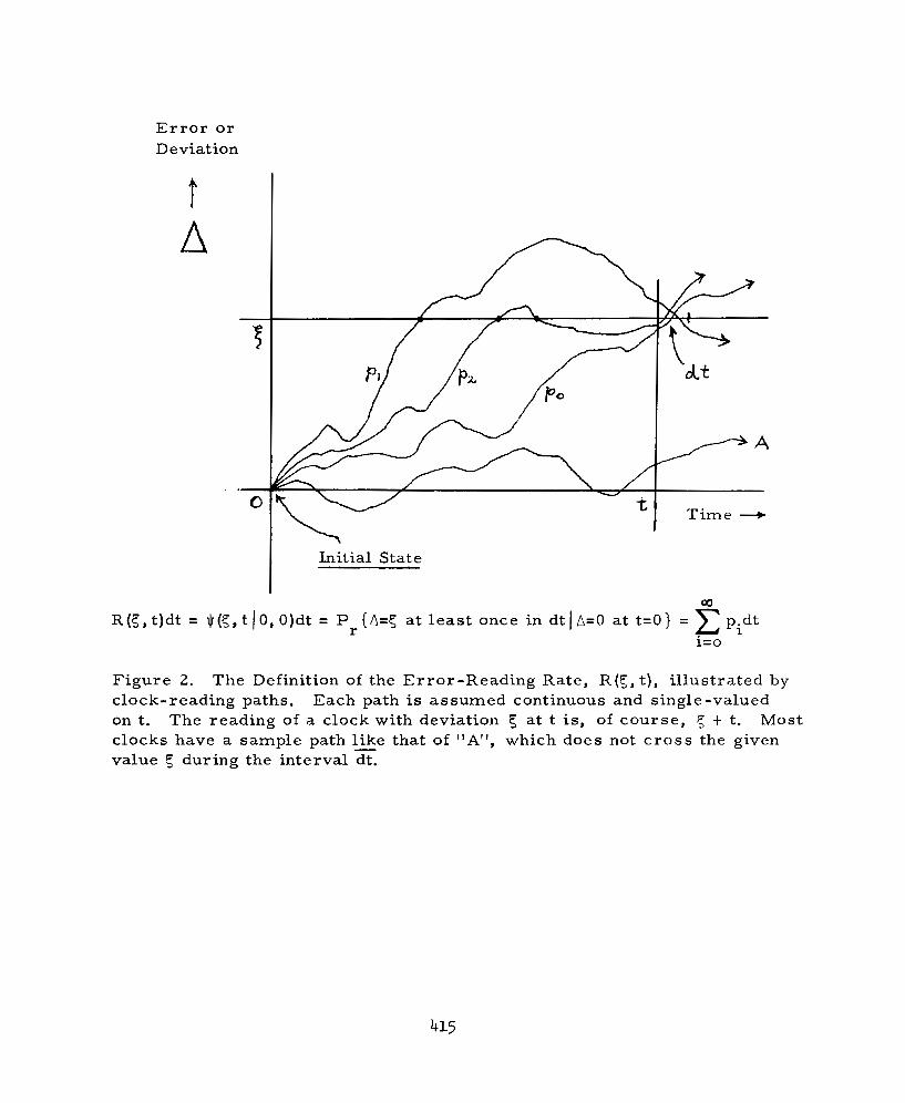
Now, imagine that, as the ensemble clocks disperse from their init ial &-function density distribution, one of the clocks is observed to go through a given deviation, 5 , in the time interval dt following t. It can do this in one of the following possible, independent ways: (See Figure 2. )

(1) its deviation might not equal 5 between 0 and t;

(2) its deviation might equal 5 just once between 0 and t;

(3) its deviation might equal 5 exactly twice between 0 and t, etc.

As we have seen, there is a probability, P(<, t IO , O;%)dt, for the first way. Call this podt. There is a lso a probability, p dt (which will be calculated in AppendixI), for the second way, and a probab' li ity, p dt, for the third, etc. The net probability that a clock takes on, or is read to have, the deviation p, at some instant in the interval dt,following t defines what we shall call the "error-reading rate function", R(?, t). In symbols

2

After evaluating p. it can be seen that the series in Equation (7) converges for all (7, t)$ (0, 0). $he definition of R depends also on the fact that the ensemble clocks originally were all set to read zero. Because of this, the function, R, could have been written $ ( c , t I O , 0). If the initial deviation of a clock had been 7' at t', then we would write $ ( c , t I S ' , t') which would emphasize that qdt is the probability of transit ion from S ' , t' to 5 , t without the condition of no deviation being equal to 5 between t' and t. Thus

For short , we shall call the "error-reading rate beginning at ( T I , t'). ' l

For the sake of more complete general i ty we a lso general ize the error probability density function, H, at this point. Le t a(? , t (0, O)d< = $ ( S , t)d< be the probability of a clock deviation, A, being between 5 and 5 t d5 at t ime t, given that its in i t ia l e r ror at t' = 0 was zero. Then we define

389

The "error probability density", 0, could have one of various forms, l ike

for example, but this is a matter to be determined empirically or on the basis of theory, or as a basic statistical hypothesis. Obviously, even though all the ensemble clocks are specified to have "paths" proceeding from the origin, they would not all read 5 sometime during a given range dt at 5 , t. An example is shown marked "A" in Figure 2. But from the definition of the time told by a clock, each path from the origin must proceed to the right (increasing t), be single-valued in 5 at each t, and cross each "vertical" line t = constant once, for t > 0.

These are rather mouthfilling probabilistic definitions of the conditional transition probability rate, P, the error-reading rate, Jl, and the error probability density, 0, all beginning at (X', t '), But, they are really needed in order to develop the theory sufficiently and carefully. It will be seen that, in spite of the seeming complication, their use assists in understanding the conditions of validity of a more simplified, yet basically important, situation for which 5 = 0, treated in the next section.

A Basic Relationship

To foreshadow the later development, it i s instructive to derive, at this point, an important relationship which i l lustrates the essential simplicity of the notions involved. Following this, it wil l then be necessary to re turn to the more general case and give additional detailed and carefully reasoned arguments to support the further development of the theory. According to an idea of one of u s (J. A. B. ), many features of the clock ensemble of the kind considered here can be character ized most s imply in terms of two other functions, p ( t ) and r(t), specifically defined for transit ions between correct readings, as follows: As in the introduction, assume that the random deviations of the clock readings from their average are t ime varying in such a way that each clock might read the correct t ime, again and again, according to some probabili ty law, That is, i f a clock reads the value t ' at the instant when the ensemble average is t', there is a conditional probability rate, p(t I t ' ) > _ O that the clock will again read the "correct" time, t, but not read the correct value at any intervening instant. Moreover, it is convenient for the moment to assume that this probabili ty rate is stationary, in the wide sense that p depends only on the difference, t - t', that is,

p(t It') = p ( t - t ' ) .

Stochastically, then, we shall regard

p ( t - t ' )dt

as the conditional probability that a clock in the ensemble has a c o r r e c t reading between times t and t t dt, on the condition that it did read the co r rec t t ime t', at an ear l ie r t ime t', but did not read the correct time between t' and t.

This conditional probability is re la ted to a probability rate function, r (t). The differ entia1

is to be regarded as the probability that an ensemble clock has a c o r r e c t reading when the ensemble is observed between the t imes t ' and t' t dt. W e shall call r(t) the "correct-reading" rate of the ensemble.

Because of the hypothesized initial b-function distribution, it is only after the instant t' = 0, that a clock can again read "correctly. " Subse- quently, the probability that a clock reads correct ly at t ime t' and again shows the correct t ime t at a later moment, t, but not in between, is

r ( t ' ) p (t-t')dtdt', t 3'.

Now, at time t 2 0, the total probability that an ensemble clock reads correctly sometime in the interval dt must equal the probability

that it reads correctly during dt after time t,having also read zero at t = 0 (but not in between), plus the probability that it did read correctly in any of the intervals dt ' at all t imes, t', between 0 and t, but did not read correct ly between t' and t, that is,

I t r ( t t ) p (t-t')dt'dt.

Thus, we arrive at the integral equation relating r(t) and p (t):

t r(t) = p ( t ) t i r ( t ' ) p ( t - t l ) d t ' .

This is the simple result sought. It is one form of a standard "renewal equation", as in the theory of probability (Feller, 1966c and 1967).

It is, of course, possible to proceed from this point strictly analytically and investigate the possible solution pairs, p ( t ) and r(t), of Equation (13). But in order to be able to use this basic relation with more assurance, and not make unwarranted inferences about extending its range of application, we first derive, under less restrictive conditions, more general equations involving the functions, 0, 4, and P introduced previously. It will then be shown how Equation (13) may be made to follow; we shall see what the conditions are under which (13), its consequences, and the assumptions leading to it remain valid.

392

Generalizations

Difficulties were at one time encountered in the attempted application of Equation (13) t o some cases of considerable importance. One such case is characterized by a reading rate, r(t), which is inversely proportional to the time, so that the convolution integral in (13) diverges. Many other, even more extremely divergent situations, have been found to be-of interest.

A way out of these difficulties has been found, but at the cost of a some- what more complex formulation. Yet, as was asserted, this too is compen- sated by a greater generality yielding a clarification of the "setting" of the description.

The derivation in the preceding section offers us a guide when viewed in the context of the definitions of the various probability functions, P, $, and 0. The quantity

P (0 , t IO, tl;O)dt

according to the section before the last is the probability of finding a n ensemble clock to have a correct reading during the time interval dt following t on the conditions that it read correct ly a t the earlier t ime t', but did not read correctly between t' and t. But the statements already made about the' probability, p(t I t ' )dt {without the specializatibn to stationarity), show that

p(t It', = P(0, t io, t';O).

Similarly, one notes that

is an equally valid identification. This formally establishes a connection and furnishes more motivation to generalize the basic idea summed up in Equation (13). Briefly, the direction of this generalization may be indicated in the form of a question: "What has the fact that clocks a r e often read to have the same or different errors many t imes between different moments to do with its conditional probabilistic description? l '

Final motivation comes from thinking about the obvious but important fact that clocks ordinarily run continuously. Again, we ask: "How can this property be described probabilistically? ' l

A simple answer has recently been found for the last question. Consider the probability that a clock, which had a deviation 5' at t ime t: is l a t e r found to have the error 5 in a time interval dt, following t. As we know, this is the error-reading probability, $ ( S , t Is', t')dt. But the fact is that any clock in its transition from the reading (SI , t ') to the reading ( S , t) must a lso be found at an intermediate t ime, t"(t'<t"<t), with some error in the range d5" near ? l f . But the probability of the transition from ( S ' , t ') t o (cl', t") in

3 93

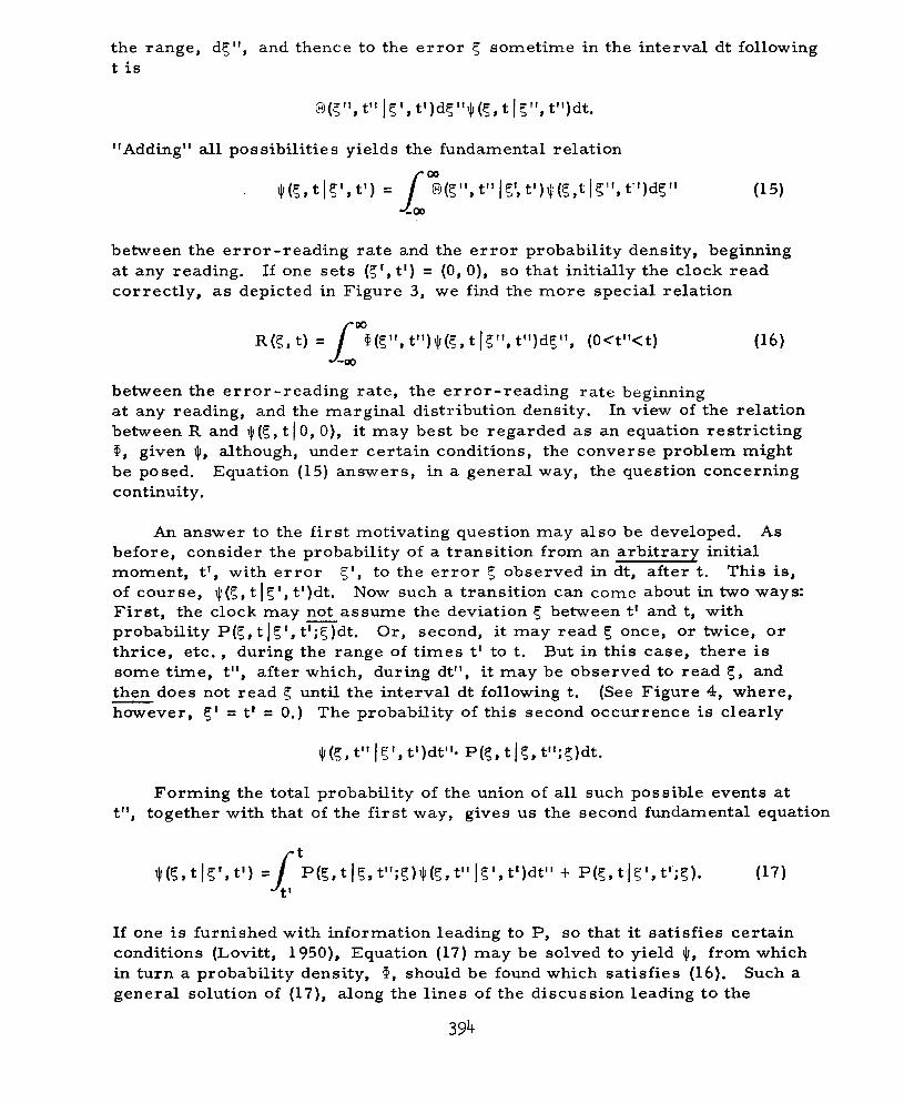
the range, dT", and thence to the error 5 sometime in the interval dt following t i s

"Adding" all possibilities yields the fundamental relation

between the error-reading rate and the error probability density, beginning at any reading. If one sets ( { l , t ') = (0, 0), so that initially the clock read correctly, as depicted in Figure 3, we find the more special relation

R(5, t) =Lm@(5If, t")JI(s, t I T f f , t")dsIf, (Oct"<t) (16)

between the error-reading rate, the error-reading rate beginning at any reading, and the marginal distribution density. In view of the relation between R and $(S, t I O , 0), it may best be regarded as an equation restricting H, given Jl, although, under certain conditions, the converse problem might be posed. Equation (15) answers, in a general way, the question concerning continuity.

An answer to the first motivating question may also be developed. As before, consider the probability of a transit ion from an arbitrary init ial moment, t', with error c ' , to the error 5 observed in dt, after t. This is, of course, $(S, t IT', t ')dt. Now such a transition can come about in two ways: First, the clock may not assume the deviation 5 between t' and t, with probability P(<, t ) 5 ' , t ' ; t)dt. Or, second, it may read 5 once, or twice, or thrice, etc. , during the range of t imes t' to t. But in this case, there is some time, t", after which, during dt", it may be observed to read 5 , and then does not read 5 until the interval dt following t. (See Figure 4, where, however, 5' = t' = 0.) The probability of this second occurrence is clearly

Forming the total probability of the union of all such possible events at t", together with that of the first way, gives us the second fundamental equation

If one is furnished with information leading to P, so that it satisfies certain conditions (Lovitt, 1950), Equation (17) may be solved to yield Jl, from which in turn a probability density, Q, should be found which satisfies (16). Such a general solution of (17), along the lines of the discussion leading to the

394

Specializations

Equations (15) and (17) are necessarily valid provided one assumes the existence of the functions 0, $, and P for the stochastic processes of interest, because the equations follow directly from the definitions. Consequently, they are also of great generality and subsume many, many more specialized situations. For example, we see immediately that Equations 14 (a and b) lead to the correct-reading renewal Equation (13), i f one additionally imposes the wide-sense stationarity property of Equation (lla).

Other assumed identifications, like

- S- P(0, t) = R(0, t) = r(t) (18a)

where S is a dimensionless proportionality constant, lead to important conse- quences. This relation is suggested by the intuition that, if a clock is likely to be reading nearly correctly, then it might be proportionately.likely that it will read correctly in any short period thereafter. An investigation by Rice (Rice, 1944 and 1945) points to the reasonableness of such an assumption. An immediate result is that the dispersion, W, for the normal Gaussian diffusion case is related to the correct-reading rate, r(t) in the simple fashion:

-

- a(t) = S

VZirr(t) (1 8b)

One can show explicitly that this relation is not inconsistent with the conditions (15) and (16); nor is the more general possibility

The detailed investigation of the not unreasonable conditions under which Equations (18) are valid is, however, left for a later paper, in which the situation for transitions between incorrect readings is investigated more extensively. We assume in the remainder of this paper the applicabilty of (18).

The use of (18b) does raise some problems, however, as was mentioned in the introduction, For i f the dispersion, o(t) , is proportional to a power of t, say tl'B, then, when PCO, and we use the relation of a( t ) to the correct- reading rate, r(t), the convolution integral in Equation (13) has no meaning.

The range of validity of the stationarity condition (lla) is another question for investigation. Let us first extend it, a s follows: In Equation (17), set 5 ' = t ' = 0, use (18c) and assume that the conditional probability rate, P, has the wide-sense stationarity property, and is expressible in te rms of a new function, P 5 1 1 1 .

395

(1 9 )

This specialization leads to the "stationary proportional error-reading rate" equation

rt

Now, P , (t I5)dt is the probability that a t ime interval t is taken for the e r ro r t r ansg ion

( A = { ' ) + ( A = S)(sometime in dt),

given that A 4 5 during the interval t. The corresponding random variable, T, the time taken for the transition 5 ' 3 , could therefore possess a probabil- ity distribution, specified by the density P (t 15); o r it may be a "defective" random variable (Feller, 1966d). (See EqSHtions 21c and d. ). In any event, it is reasonable to assume that

exists, and is less than or, equal to unity. This assumption can be regarded as par t of the specification of a "stationary proportional error-reading rate" process. Here f(5'15) is a new function.

Equation (20) itself is in the form of the general renewal equation with a parameter , 5 . As such, it is still very general. Some of its properties will be investigated in the later paper, There are excellent indications, because of the exponential "convergence" factor in the Gaussian form of @ (Equation

(4a)) that this equation will be applicable to situations where r(t) diverges badly as t 4 .

Naturally, as 5-0, we identify P (t IO) with p ( t ) , the probability density that T = t for transit ions between successive correct readings. For this case, Equation (20) reduces to the correct-reading renewal Equation (13). Because p ( t ) is a probability density, the condition (ala) specializes to the form

0

/%,(t 1O)dt = k:(t)dt = f ( O 1 0 ) l l 0

so that, by definition, if T is a proper random variable

f(O10) = 1

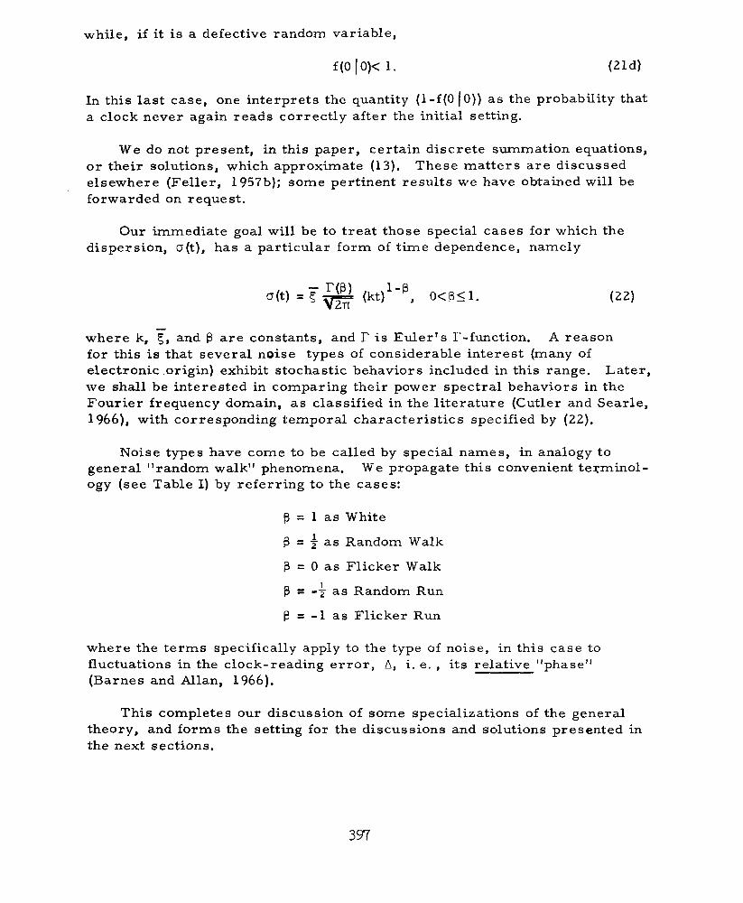
while, i f it is a defective random variable,

In this last case, one interprets the quantity ( l - f ( O IO)) as the probability that a clock never again reads correctly after the initial setting.

W e do not present, in this paper, certain discrete summation equations, or their solutions, which approximate (13). These matters are discussed elsewhere (Feller, 1957b); some pertinent results we have obtained will be forwarded on request.

Our immediate goal will be to treat those special cases for which the dispersion, cr(t), has a particular form of time dependence, namely

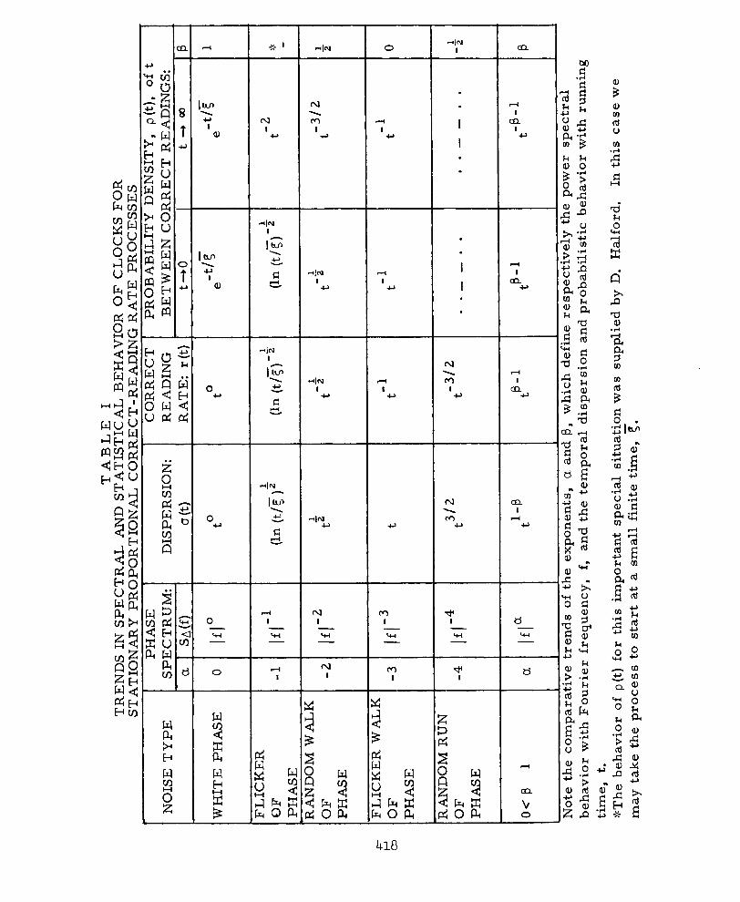
where k, 5 , and B are constants, and l? is Euler's r-function. A reason for this is that several noise types of considerable interest (many of electronic origin) exhibit stochastic behaviors included in this range. Later, we shall be interested in comparing their power spectral behaviors in the Fourier frequency domain, as classified in the literature (Cutler and Searle, 19661, with corresponding temporal characteristics specified by (22).

Noise types have come to be called by special names, in analogy to general "random walk" phenomena. We propagate this convenient tesminol- ogy (see Table I) by referring to the cases:

f3 = 1 as White

B = z a s Random Walk

B = 0 as Flicker Walk

p = -2 a s Random Run

= -1 as Flicker Run

1

1

where the terms specifically apply to the type of noise, in this case to fluctuations in the clock-reading error, A , i. e. , its relative "phase" (Barnes and Allan, 1966).

This completes our discussion of some specializations of the general theory, and forms the setting for the discussions and solutions presented in the next sections.

397

Renewal Process Properties for Correct-Reading Situations

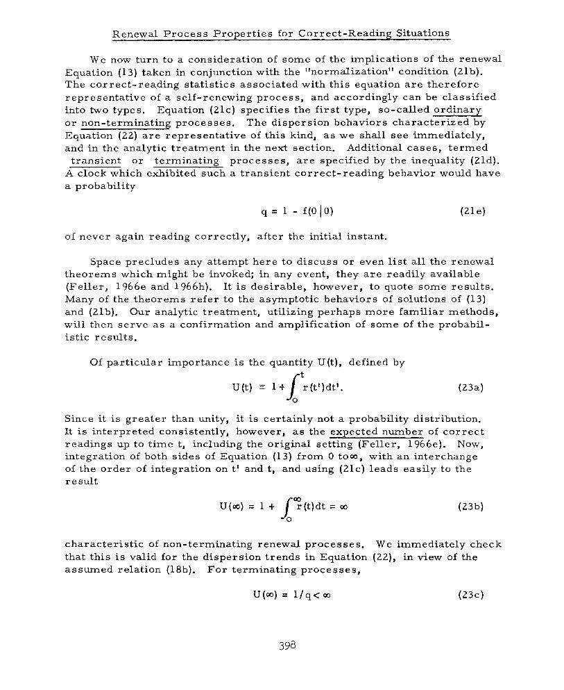
We now turn to a consideration of some of the implications of the renewal Equation (13) taken in conjunction with the "normalization" condition (21b). The correct-reading statist ics associated with this equation are therefore representat ive of a self-renewing process, and accordingly can be classified into two types. Equation (21c) specifies the first type, so-called ordinary or non-terminat ing processes . The dispers ion behaviors character ized by Equation (22) are representat ive of this kind, as we shall see immediately, and in the analytic treatment in the next section. Additional cases, termed

t ransient or terminat ing processes , are specif ied by the inequality (21d). A clock which exhibited such a transient correct-reading behavior would have a probability

of never again reading correctly, after the init ial instant.

Space precludes any attempt here to discuss or even l ist al l the renewal theorems which might be invoked; in any event, they are readily available (Feller, 1966e and 19661.1). It is desirable, however, to quote some results. Many of the theorems refer to the asymptotic behaviors of solutions of (1 3) and (21b). Our analytic treatment, utilizing perhaps more familiar methods, wil l then serve as a confirmation and amplification of some of the probabil- is t ic resul ts .

Of par t icular importance is the quantity U(t) , defined by

(23a)

Since it is greater than unity, it is certainly not a probability distribution. It is interpreted consistently, however, as the expected number of co r rec t readings up to t ime t, including the original setting (Feller, 1966e). Now, integration of both sides of Equation (13) from 0 tom, with an interchange of the order of integration on t' and t, and using (21c) leads easily to the resu l t

charac te r i s t ic of non-terminating renewal processes. W e immediately check that this is valid for the dispersion trends in Equation (22), in view of the assumed relation (18b). For terminating processes,

398

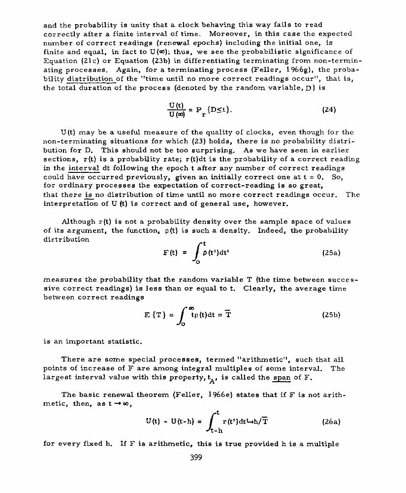
and the probability is unity that a clock behaving this way fails to read correctly after a finite interval of time. Moreover, in this case the expected number of correct readings (renewal epochs) including the initial one, is finite and equal, in fact to U(00); thus, we see the probabilistic significance of Equation (21c) o r Equation (23b) in differentiating terminating from non-termin- ating processes. Again, for a terminating process (Feller, 1966g), the proba- bility distribution of the "time until no more correct readings occur", that is, the total duration of the process (denoted by the random variable, D ) is

U ( t ) may be a useful measure of the quality of clocks, even though for the non-terminating situations for which (23) holds, there is no probability distri- bution for D. This should not be too surprising. As we have seen in earlier sections, r(t) is a probability rate; r(t)dt is the probability of a correct reading in the interval dt following the epoch t after any number of correct readings could have occurred previously, given an initially correct one at t = 0. So, for ordinary processes the expectation of correct-reading is so great, that there is no distribution of time until no more correct readings occur. The interpretation of U (t) is correct and of general use, however.

Although r(t) is not a probability density over the sample space of values of its argument, the function, p ( t ) is such a density. Indeed, the probability distribution rt

F(t) = l p(t')dt'

measures the probability that the random variable T (the time between succes- sive correct readings) is less than or equal to t. Clearly, the average time between correct readings

E {T} = l ? p ( t ) d t = T

is an important statistic.

There are some special processes, termed "arithmetic", such that all points of increase of F a r e among integral multiples of some interval. The largest interval value with this property, t is called the span of F. A'

The basic renewal theorem (Feller, 1966e) states that i f F is not arith- metic, then, as t 3 a,

U(t) - U(t-h) l ; r ( t l )d tbh /T ( 2 6 4

for every fixed h. If F is arithmetic, this is true provided h is a multiple

399

of the span, t It can be shown that (26a) is equivalent to stating that, for the non-arithmetic case:

A'

r ( t )4$ L; ( t )d t = f ( o , I T 0 )

a s t + m . The power of application of the renewal theory becomes immediately obvious. For our special cases of interest, except for "white" phase noise for which B = 1 , a(t)-, m , and hence ( i f S is finite), r(t)+ 0, a s t * m (see Equation (18b)). Then, the form (26b)of the basic theorem shows that

In words, "The expected length of t ime between successive correct c lock readings is infinite except for the case of white phase noise. In this case,

since r (t) = -+; is a constant, and f ( O IO) = 1 , -

In view of the interpretation of U( t ) , the basic renewal theorem asser ts also that , i f F is non-arithmetic, the expected number of cor rec t read ings within any time interval of fixed length, h, approaches h/T, in the limit of very long times. Since, for white deviation noise, r is a constant, this limit is already reached in any f inite t ime, But this statement then coincides with the definition of a simple Poisson process. Thus, the probabili ty of an interval value, t, between successive correct readings for white correct- reading noise should vary exponentially. We shall verify this in the next section.

Finally, it is of interest to note without discussion two further important resu l t s of renewal theory. We first define the variance of the times between successive correct readings:

O 2 T = l ? p ( t ) d t - -2 T .

Then, one can show (Feller, 1966f) that 2 -2

t aT t T 0 5 U ( t ) -T-+

2 5

as t +m. Thus, i f D and T exist , then for long t imes the number of c o r r e c t readings, N , up to t ime t (excluding the initial moment), has a normal-

400

- T

t

Gaussian distribution with expectation t/T and variance equal to

t aT/T . 2 - 3

Unfortunately, we seem to be often faced with situations for which T and OT do not exist. There have been investigations of such cases, some of which we have not yet had time to assimilate (Feller, 1949 and Mandelbrot, 1967). Others have used alternative approaches and approximations to noise processes which involve statistical procedures where only finite samples and statistics occur (Halford, 1968). At any rate, we now turn to an analytic treatment of Equation (13). This will amplify and verify some of the statements made in this section.

401

Some Solutions and Their Properties

We have specified the dispersion of our ensemble clocks according to Equation (22), and the correct-reading rate is determined by (18b). Thus, we are lef t wi th the problem of determining p(t) given

The magnitudes of the proportionali ty constants are ei ther to be determined empir ical ly , or by a more detailed physical theory.

Of course, the converse theoret ical problem is often encountered. Indeed, we have indicated a quite general form of solution for the general error-read- ing rate R(<, t) in Equation (7) , as explicitly developed in Appendix I. Simi- lar ly , one can express r(t) a s a sum of repeated autoconvolutions of p ( t ) :

t r(t) = p(t) t dt 'p( t - t ' )p( t ' ) t dt"p(t'-t")p(t") t .(31)

The interpretation of the nth term of t h i s s e r i e s is obvious in view of what is said in Appendix I. It is the probability density of a correct reading f o l l o w i n e i m e t given a correct one ini t ia l ly and (n- l ) correct ones in the interval O t . Hence, (31) simply is a formal statement of the definition of r (t) and is the unique solution of (13), given p ( t ) .

Even so, it is instructive to verify (31) by analytic methods, for this points the way toward finding p ( t ) explicitly, given r(t). Therefore, take the one-sided Laplace transform of both sides of Equation (13), using the general property that the Laplace t ransform of the convolution of two functions is the product of their Laplace transforms, Denote by ?(X) the ordinary Laplace t ransform

a0 L1

r(X) = 1 emXtr (t)dt 0

of r(t). Similarly, for F(A). Then, we have

- P r = 1 -F

o r 5 r F = - l t?

402

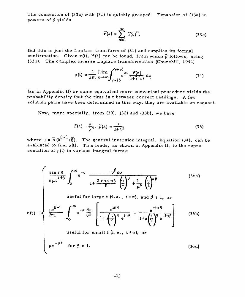
The connection of (33a) with (31) is quickly grasped. Expansion of (33a) in powers of F yields

n= 1

But this is just the Laplace-transform of (31) and supplies its formal confirmation. Given r(t), yfi) can be found, from which F follows, using (33b). The complex inverse Laplace transformation (Churchill, 1944)

(as in Appendix 11) or some equivalent more convenient procedure yields the probability density that the time is t between correct readings. A few solution pairs have been determined in this way; they are available on request.

Now, more specially, from (30), (32) and (33b), we have

where p = S (kP- l /T). The general inversion integral, Equation (34) , can be evaluated to find p( t ) . This leads, as shown in Appendix 11, to the repre- sentation of p(t) in various integral form s:

-

I useful for large t (i. e., t + m), and /3 * 1, o r

I useful for small t (i, e. , t - + o ) , or

403

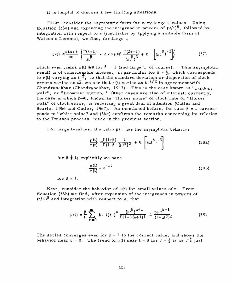
It is helpful to discuss a few limiting situations.

First, consider the asymptotic form for very large t-values. Using Equation (36a) and expanding the integrand in powers of (v/t)B, followed by integration with respect to v (justifiable by applying a suitable form of Watson's Lemma), we f ind, for large t,

which even yields p ( t ) E O for = 1 (and large t, of course). This asymptotic resu l t is of consideqable interest , in particular for B = T , which corresponds to r(t) varying as t;", so that the standard deviation or dispersion of clock e r r o r s v a r i e s a s t t ; we see that p( t ) var ies as t-3/2 in agreement with Chandrasekhar (Chandrasekhar, 1943). This is the case known as "random walk", or "Brownian motion. ' I Other ca ses a r e a l so of interest ; current ly , the case in which 840, known as "flicker noise" of c lock ra te or "f l icker walk" of c lock e r ro r , is receiving a great deal of attention (Cutler and Searle , l966 and Cutler, 1967). As mentioned before, the case = 1 c o r r e s - ponds to "white noise" and (36c) confirms the remarks concerning i ts relation to the Poisson process , made in the previous sect ion.

1

For large t -values , the ra t io p / r has the asymptotic behavior

fo r @ $: 1; explicitly we have

for B = 1.

Next, consider the behavior of p ( t ) for small values of t. F r o m Equation (36b) we find, after expansion of the integrands in powers of (t/v)B and integration with respect to v, that

The ser ies converges even for B = 1 to the correct value, and shoys the behavior near = 0. The t rend of p ( t ) near t = 0 for B = 2 is a s t-2 jus t 1

404

as fo r r(t). Indeed, the ratio ( p / r ) has the interesting behavior

This is not so for large t, and should only be applied for B>O, a s t approaches zero.

Note that the function describing the behavior of p for small t and small B also gives the correct asymptotic behavior for large t and small @ - - hence one guesses that it m a y be a close approximation for all t. This statement is strengthened by the observation that

in agreement with (21c).

As a mat te r of fact, the expression given in (39)

is a fair ly good approximation to p , even for values of B approaching unity. It has the correct behavior , for both large and small t, for @ = z, and for small t, with = 1. An even better expression, since it yields a more re f ined approximation to p (t) for positive B 51, and all t, is

1

with an adjustable parameter, n. It is easy to see that Fdt = 1. This may

( 3 0 ) , one should remember that p = T((k@'l /F). bear further investigation. In using formulas ( 3 6 ) - (42) conjuntion with

Table I summarizes the l imit ing t rends for large and small t-values, with other entries corresponding to important special fluctuation or noise types. It shows a comparison of these t rends with power spectral behaviors of cer ta in common noise processes. Assuming ergodicity, the power spectral density, S,(f), is defined in terms of the temporal t rend of a s ample e r ro r p rocess ,

A b ) , by /-m

Sa(f) = 2 joRA(t) cos 2TTft dt

40 5

where R (t) is the auto-correlation function of the sample, computed from a m

Lim 1 I

RA(t) = T+oo E L A(t')A(tl+t)dtl.

In the present paper, no statistical relation has been established by logical derivation between the power spectral density functions so defined and the quantities D, p, and r, of primary interest here. However, other studies (Allan, 1966) have delved into this question, and have related the trends of SA(f) to those of a(t). Some results are summarized in Table I, and enable the comparisons of trends to be made. The correspondences shown depend specifically on the "stationary proportional correct-reading rate" process hypothesis. In many cases of interest, as the Table indicates, the power spectral density in the Fourier frequency domain has been a statistic applicable to processes otherwise found difficult to analyze.

In the Table the exponents, a, of the absolute Fourier frequency If I , in the expressions listed for the power spectral density, SA(f), and the corres- ponding temporal exponents, 8 , are apparently related by

a = 28 - 3 (44)

for a I -2. This may, however, be fortuitous. Analogous relations between Fourier frequency and temporal (averaging time) behaviors were obtained by D. Allan in the foregoing reference in connection with the statistical analysis of atomic clock and oscillator data.

Conclusions

From the foregoing analyses we conclude that the renewal Equation (13) relating the distribution of times between correct readings to the correct- reading rate, leads to a theoretical description of use for white-noise and random-walk-noise clock reading processes. It is indicative of the correct relationship for the limiting case of flicker-walk of phase, but is inadequate to describe lower orde-r noises, that is, B < 0, whose dispersion rates accelerate from zero. It is likely that a more general approach, utilizing more fully the general probability functions JI, P, and 0, introduced initially, will be needed. As a minimum requirement, investigation of the more general renewal Equation (20), applicable to non-zero reading deviations, seems in order. Perhaps the most important result of the present investigation is the recognition that many important clock processes are stochastic processes of standard renewal type.

The writers express their appreciation to Professor W. Feller, to Dr. D. Halford, and to Dr. S. Jarvis for many useful and stimulating suggestions and discussions. They also express thanks to Mrs. J. West for secretarial assistance in preparing the paper,

406

APPENDIX I

Solution of the Error-Reading Rate Equation (17)

We find a solution for $ ( S , t l g ' , t ') by the method of iteration and succes- sive approximations. Let the zeroth approximation be

Then, let the next approximation be

Proof that Jrn converges to a unique solution, Jr, a s n d m , i f P sat isf ies cer- tain conditions, will be omitted here for brevity (Lovitt, 1950). If we set { I = t' = 0, then, as n - 00, 1$~(5 , t l0,O) approaches the error-reading rate function, R(<, t), as defined in (7). We see that the probability, pldt, has the form t

pldt = 1 P(<, t 15, t";{)dt"P(?, t" ( 0 , 0;s)dt.

It is the probability that a clock, initially reading correctly, will have a devia- tion, 5 , in the time interval, dt, following t, having had the error, 5 , just once between 0 and t. From this statement, the interpretation of each of the terms in the infinite series for $ ( S , t IT', t') becomes obvious. The meaning of each of the conditional probabilities, $,(I, t Is1, t ')dt is also c lear .

407

APPENDIX II

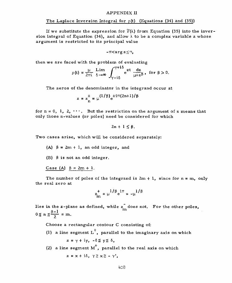
The Laplace Inversion Integral for p ( t ) (Equations (34) and (35))

If we substitute the expression for ?(h) from Equation (35) into the inver- sion integral of Equation (34), and allow X to be a complex variable z whose argument is res t r ic ted to its principal value

- n < a r g z l n ,

then we are faced with the problem of evaluating

U Lim F \"I - 2rri

I -"

The zeros of the denominator in the integrand occur at

* ( I / s ) * in(2nt l ) /g z = z = p n e

for n = 0, 1, 2, * . But the restriction on the argument of z means that only those n-values (or poles) need be considered for which

2 n t 1 < B .

Two cases arise, which will be considered separately:

(A) p = 2m t 1, an odd integer, and

(B) B is not an odd integer.

Case (A) B = 2m t 1. . . .

The number of poles of the integrand is 2m t 1, since for n = m, only the rea l zero at

l ies in the z-plane as defined, while B - 1 O ~ n ~ - = m . 2

Choose a rectangular contour C

(1) a line segment L , parallel t

z = y t iy, -6s y s 6 ,

z does not. For the other poles, m

consisting of:

to the imaginary axis on which

40 8

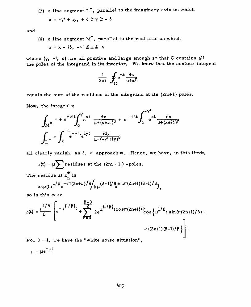
where (y, y', 6 ) are all positive and large enough so that C contains all the poles of the integrand in its interior. W e know that the contour integral

equals the sum of the residues of the integrand at its (2mtl) poles.

all clearly vanish, as 6, y t approach m . Hence, we have, in this limit,

p ( t ) = p x r e s i d u e s a t t h e (2m t 1 ) -poles.

The residue at Z* is n

so in this case

-n (2n t1 ) (~ -1 ) /~} . J For B = 1, we have the "white noise situation",

409

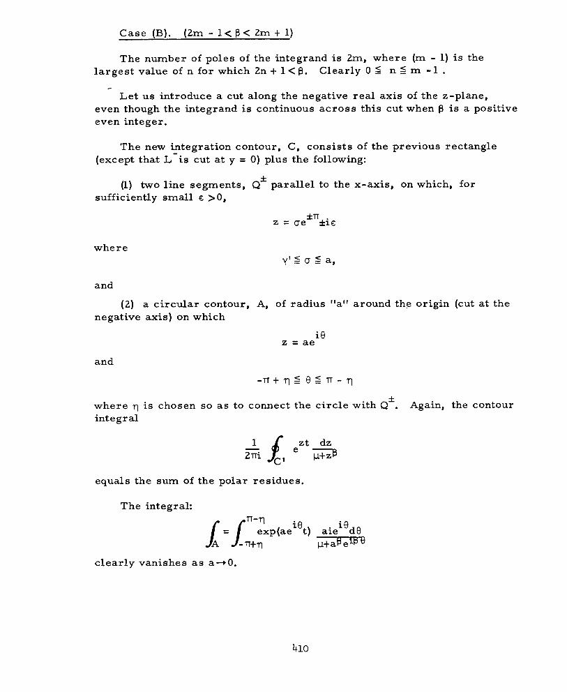
Case (B). (2m - 1 < B 2m + 1)

The number of poles of the integrand is 2m, where (m - 1) is the largest value of n for which 2n t 1 < 8 . Clearly 0 9 n I m - 1 .

e

Let us introduce a cut along the negative real axis of the z-plane, even though the integrand is continuous across this cut when fl is a positive even integer.

The new integration contour, C, consists of the previous rectangle (except that L-is cut at y = 0) plus the following:

(1) two line segments, Q parallel to the x-axis, on which, for f

sufficiently small c >0,

where y ' S 0 2 a,

and

(2) a circular contour, A, of radius rlalr around the origin (cut at the negative axis) on which

i e z = ae

where q is chosen so as to connect the circle with Q . Again, the contour integral

f

equals the s u m of the polar residues.

The integral: L = l:>(aeiet) aieiedO p+ aP eip 9

clearly vanishes as a+0.

The integrals along Q are: f

As .S approaches zero, these integrals become equal to

and the integral along L- has its former value.

Let y' and 6 become infinite as before, and let "a" approach zero,

Then, in this limit

p(t) = p c (residues at the 2m-poles) t I(t)

where

as in the text, Equation (36a), while a simple rearrangement of factors in the split terms leads immediately, with this substitution, to Equation (36b). In this we assume that O < 8<1 , so that the residue s u m does not contribute. When @ = 1, we get the white noise form for p ( t ) , Equation (36c), and i f B>1 and not an odd integer, we have the formula

CI p ( t ) = 2- cos (n-) 2n t l cos 1 pi sin (n- 2ntl) 8 B

Note that the constant, p, equals ;kp'l /F. The writers express their thanks to Dr. S, Jarvis for assistance with the

contour integrations in this Appendix.

References

Allan, D. W. ( l966) , Statist ics of atomic frequency standards, Proc. IEEE, 54, NO. 2, 221-230. 3

Barnes , J. A., D. W. Allan, and D. H. Andrews (1965), The NBS-A-Time Scale, its generation and dissemination, IEEE Trans. Instr. Measr., IM-14, 228-232.

Barnes, J. A. , and D, W. Allan (1966), A statist ical model of f l icker noise, Proc. IEEE, 54, No. 2, 176-178. -

Barnes, J. A. (1967), The development of an international atomic time scale, Proc. IEEE, 55, No. 6, 822-826. -

Barnes, J. A . , and D. W. Allan (1967), An approach to the prediction of coordinated universal t ime, Frequency, 5, No. 6, 15-20. -

Chandresekhar, S. (1943), Rev. Mod. Phys., 15, No. 1, 1-89.

Churchill, R. V. (1944), Modern Operational Mat:hematics in Engineering, 157 and ff (McGraw-Hill Book Co., New York, N. Y. ).

Cutler , L. and C. Searle (1966), Some aspects of the theory and measurement of frequency fluctuations in frequency standards, Proc. IEEE, 54, No, 2, 136- 154.

-

Cutler, L. (1967), P r e s e n t status in short term f requency s tabi l i ty , Frequency, 5, No. 5, 13-15. -

Fe l l e r , W. (1949), Fluctuation theory of recurrent events , Trans. Amer. Math. Soc. , c, 98- l 1 9.

Fe l l e r , W. (1957a), An Introduction to Probability Theory and Its Applications, Vol. I, 283 (John Wi ley and Sons, Inc., New York, N. Y. ).

Fe l l e r , W. (1957b), Vol I, 285 and ff.

Fe l le r , W. (1957c), Vol I, 290.

Fe l l e r , W. (1966a), An Introduction to Probability Theory and Its Applications, Vol. 11, 181 (John Wiley and Sons, Inc., New York, N. Y. ).

Fe l l e r , W. (1966b), Vol U, 182.

Fe l l e r , W. (1966c), Vol 11, 183.

Fe l l e r , W. (1966d), Vol II, 184.

Fe l l e r , W. (1966e), Vol 11, 346 and ff.

Fe l l e r , W. (1966f), Vol 11, 357.

F e l l e r , W. (1966g), Vol 11, 360 and f f .

Fe l l e r , W. (1966h), Vol 11, 441 and f f .

Fe l l e r , W. (1967), Private communication, October 1967.

Halford, D. (1 968), A general mechanical model for I f I a spectral densi ty ransom noise with special reference to f l icker noise l / I f l , P roc. IEEE, 56, NO. 3, 251-258. -

Lovitt, W. V. (1950), Linear Integral Equations, Chap. I1 (Dover Publica- tions, New York, N. Y. ).

Mandelbrot, B. (1967), Some noises with l / f spectrum, a bridge between direct current and white noise, IEEE Trans, Inform. Theory, IT-13, NO. 2, 289-298.

Rice, S. 0. (1945), Mathematical analysis of random noise, Bell System Tech. J. , 24, 46-156. -

414

E r r o r o r Deviation

f a

5

.- 0

Initial State

Time +

Qd

R(5, t )dt = $(<,t(O,O)dt = Pr{A=< at least once in dtlA=O a t t=o} =c p.dt ~-

l i=o

Figure 2. The Definition of the Error-Reading Rate, R(<, t), i l lustrated by clock-reading paths. Each path is assumed continuous and single-valued on t. The reading of a clock with deviation 5 at t is, of course, 5 t t. Most clocks have a sample path like that of "A", which does not cross the given value 5 during the interval dt.

-

definition of R (Equation (7)), is presented in Appendix I. Equation (17) is a generalization of (13); it answers the question concerning $, the "e r ror - reading rate, beginning at <', t' ", and the conditional transition probability ra te , P.

3- E r r o r

n p" 5 -

C

7 L

-t " t Time

Figure 3. The Continuity of Clock-Readings relates the marginal distribution to the error-reading rate and the error-reading rate beginning at an arbitrary reading.

416

t A

Deviation

r -

0 -

A f 5 on t"t

t" Time

t

Figure 4. Types of Clock Transitions beginning with a correct in i t ia l reading.

-W I 0 dl

4

I c,

\ N

m I c,

4 I

m I c,

4 I dl c,

4 I L)

\ N

cr) I c,

4 I ca c,

MIN I c,

4 I c,

dl 1

4 c, "'"1,

c,

N I - W - W W

N l

rr) I I

d

4

dl

L 0

418