Cliques and a New Measure of Clustering:

with Application to U.S. Domestic Airlines∗

Steve Lawford and Yll Mehmeti

ENAC, University of Toulouse

May 30, 2018

Abstract

We propose a natural generalization of the well-known clustering coefficient for triples C(3) to any number of

nodes. We give analytic formulae for the special cases of three, four, and five nodes and show, using data on

U.S. airline networks, that they have very fast runtime performance. We discuss some theoretical properties and

inherent limits of the new measure, and use it to provide insight into changes in network structure over time.

1 Introduction

Networks are ubiquitous in economics. Recent examples of their empirical application include Banerjee et al.

[4], Faris and Felmlee [12], Jackson [16] (social networks), Akbas et al. [3], Cohen-Cole et al. [7], El-Khatib et al.

[11], Hochberg et al. [14], Robinson and Stuart [22] (financial networks), and Aguirregabiria and Ho [2], Baumgarten

et al. [5], Guimera et al. [13], Lin and Ban [18], Lordan et al. [19], Ryczkowski et al. [23], Verma et al. [26] and

Wuellner et al. [27] (transportation networks). These papers formalize real-world interactions — such as information

transfer links between firms, or physical air travel routes between airports — using the tools of graph theory.

∗We are grateful to Chantal Roucolle and Tatiana Seregina for helpful comments and suggestions. Correspondence can be addressed toSteve Lawford, ENAC (DEVI), 7 avenue Edouard Belin, CS 54005, 31055, Toulouse, Cedex 4, France; email: steve.lawford@enac.fr. Theusual caveat applies. JEL classification: L14 (Transactional Relationships; Contracts and Reputation; Networks), L22 (Firm Organization andMarket Structure), L93 (Air Transportation), C65 (Miscellaneous Mathematical Tools). Keywords: Airline network, Clique, Clustering,Graph theory, Subgraph.

1

Typically, they report a selection of summary statistics to capture particular global or local aspects of the network,

including its density, distribution of node centrality, and clustering. These measures can provide insight into network

structure and dynamics, that would not be available from using other methods. Clustering is especially important

in economic networks, and captures the extent to which an individual’s contacts are themselves linked. There is

evidence that a high level of clustering is related to cooperative social behaviour and beneficial information and

reputation transfer, and that many real-world networks exhibit higher clustering than if links were formed at random

(e.g. Newman [21], Jackson [15, 16] and references therein).

One widely used measure of clustering in a network (graph) is the overall clustering coefficient which is defined

in Newman [21, equation (3.3)] as, in our notation,

C(3) =3×number of triangles in the networknumber of connected triples of vertices

, (1)

where a connected triple is a set of three distinct nodes u, v and w, such that at least two of the possible edges

between them exist. In other words, how often are an individual’s friends also friends with one another, on average,

across the entire network? Since C(3) is based upon connected triples of nodes, it is natural to ask whether a similar

measure can be derived for any number of nodes. In this paper, we make the following specific contributions:

• We propose a new generalized clustering coefficient C(b), based upon connected groups of b nodes, which

nests the standard clustering coefficient C(3). We develop a very fast analytic implementation for connected

groups of three, four and five nodes, that we show to be up to 2,000 times faster than a naıve nested loop

algorithm, for some small real-world networks.

• We examine some theoretical properties of C(b) and show that it will become prohibitively difficult to compute

C(b) efficiently as b increases, even using analytic formulae, since these will become too cumbersome to

derive. Using data on U.S. airline networks over time, we show that C(b) can be highly correlated across b,

and with network density, which may reduce its practical benefits on some datasets of interest. It is not yet

known whether this high correlation holds generally for large classes of networks.

All analytic formulae that we use, and several proofs, are collected in Appendix A, and a supporting table of

correlation coefficients and additional figures are reported in Appendix B.

2

2 Graph Theory and Clustering

We briefly review some relevant tools of graph theory. Important monographs include Diestel [10] (mathematics),

Jackson [15] (economics of social networks) and Jungnickel [17] (algorithms). A graph is an ordered pair G = (V,E)

where V and E denote the sets of nodes and edges of G, respectively. We use n = |V | and m = |E| to represent

the numbers of nodes and edges of G. A graph has an associated n× n adjacency matrix g, with representative

element (g)i j that takes value one when an edge is present between nodes i and j, and zero otherwise. We also use

(i, j) ∈ E to denote an edge between nodes i and j, and say that they are directly-connected. A graph is simple and

unweighted if (g)ii = 0 (no self-links) and (g)i j ∈ {0,1} (no pair of nodes is linked by more than one edge, or by

an edge with a weight that is different from one). A graph is undirected if (g)i j = (g) ji. A walk between nodes

i and j is a sequence of edges {(ir, ir+1)}r=1,...,R such that i1 = i and iR+1 = j, and a path is a walk with distinct

nodes. A graph is connected if there is a path between any pair of nodes i and j. In this paper, we consider simple,

unweighted, undirected and connected graphs.

The degree ki = ∑ j(g)i j is the number of nodes that are directly-connected to node i, and the (1-degree)

neighbourhood of node i in G, denoted by ΓG(i) = { j : (i, j) ∈ E}, is the set of all nodes that are directly-connected

to i. The density d(G) = 2m/n(n− 1) is the number of edges in G relative to the maximum possible number of

edges in a graph with n nodes. A graph G′ = (V ′,E ′) is a subgraph of G if V ′ ⊆ V and E ′ ⊆ E where (i, j) ∈ E ′

implies that i, j ∈V ′. A spanning tree on G is a connected subgraph with nodes V and the minimum possible number

of edges m = n−1. A complete graph on n nodes, Kn, has all possible edges, and a complete subgraph on b nodes is

called a b-clique. A maximal clique is a clique that cannot be made larger by the addition of another node in G with

its associated edges, while preserving the complete-connectivity of the clique. A maximum clique is a (maximal)

clique of the largest possible size in G, and the clique number w(G) of the graph G is the number of nodes in a

maximum clique in G. Let G(n, p) be an Erdos-Renyi random graph with nodes V = {1, . . . ,n} and edges that

arise independently with constant probability p. Using the notation of Agasse-Duval and Lawford [1], we refer

to particular topological subgraphs by M(b)a , where b is the number of nodes in the subgraph, and a is the decimal

representation of the smallest binary number derived from a row-by-row reading of the upper triangles of each

adjacency matrix g from the set of all topologically-identical subgraphs on the same b nodes.

3

2.1 Analytic formulae for a generalized clustering coefficient

The clustering coefficient C(3) is bounded by 0≤C(3)≤ 1, attaining the minimum when there are no triangles in

the graph, and taking the maximum value for a complete graph Kn. Since each triangle contains three triples of

nodes, a factor of three appears in the numerator. A naıve algorithm that considers every distinct triple of nodes in G,

based on nested loops, will run in O(n3) time. However, it is easy to write down an analytic version of C(3), using

the nested subgraph enumeration formulae in Agasse-Duval and Lawford [1, equations (1) and (2)]:

C(3) =3 |M(3)

7 ||M(3)

3 |=

tr(g3)

∑i ki(ki−1), (2)

and where C(3) makes explicit the definition of clustering in terms of triples M(3)3 and triangles M(3)

7 .

If we instead interpret (2) as the average probability that any three connected nodes in a graph are also completely-

connected, then a natural generalization follows to any number b of nodes, such that 3 ≤ b ≤ n. We define the

generalized clustering coefficient as follows:

C(b) =a(b)×number of b-cliques in Gnumber of b-spanning trees in G

, (3)

where Cayley’s formula a(b) = bb−2 gives the number of spanning trees in Kb, and ensures that 0 ≤ C(b) ≤ 1.

Clearly, C(b) nests C(3), and equals zero if and only if there are no b-cliques in the graph. Moreover, we show

Proposition 2.1. Let G be a connected graph with at least b nodes (b ≥ 3). Then C(b) = 1 if and only if G is

complete.

A naıve algorithm for (3), based on nested loops, will run in O(nb) time. For example, the denominator of (3)

can be calculated by considering every distinct set of b nodes in G, and counting the number of spanning trees

on each subgraph. This will be excessively slow. If we instead think of C(b) as a measure of the prevalence of

b-cliques relative to all connected groups of b nodes, then it is clear that we can use analytic subgraph enumeration

for counting the cliques and the spanning trees for the special cases C(4) and C(5), in the same way as for (2):

C(4) =16 |M(4)

63 ||M(4)

11 |+ |M(4)13 |

=4 ∑i tr(g3

−i)

∑i ki(ki−1)(ki−2)+6 ∑(i, j)∈E(ki−1)(k j−1)−3 tr(g3). (4)

4

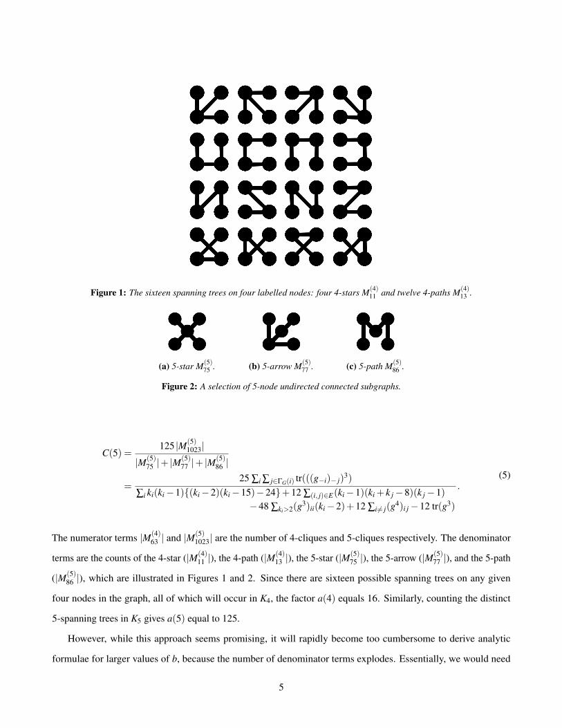
Figure 1: The sixteen spanning trees on four labelled nodes: four 4-stars M(4)11 and twelve 4-paths M(4)

13 .

(a) 5-star M(5)75 . (b) 5-arrow M(5)

77 . (c) 5-path M(5)86 .

Figure 2: A selection of 5-node undirected connected subgraphs.

C(5) =125 |M(5)

1023||M(5)

75 |+ |M(5)77 |+ |M

(5)86 |

=25 ∑i ∑ j∈ΓG(i) tr(((g−i)− j)

3)

∑i ki(ki−1){(ki−2)(ki−15)−24}+12 ∑(i, j)∈E(ki−1)(ki + k j−8)(k j−1)−48 ∑ki>2(g3)ii(ki−2)+12 ∑i 6= j(g4)i j−12 tr(g3)

.(5)

The numerator terms |M(4)63 | and |M(5)

1023| are the number of 4-cliques and 5-cliques respectively. The denominator

terms are the counts of the 4-star (|M(4)11 |), the 4-path (|M(4)

13 |), the 5-star (|M(5)75 |), the 5-arrow (|M(5)

77 |), and the 5-path

(|M(5)86 |), which are illustrated in Figures 1 and 2. Since there are sixteen possible spanning trees on any given

four nodes in the graph, all of which will occur in K4, the factor a(4) equals 16. Similarly, counting the distinct

5-spanning trees in K5 gives a(5) equal to 125.

However, while this approach seems promising, it will rapidly become too cumbersome to derive analytic

formulae for larger values of b, because the number of denominator terms explodes. Essentially, we would need

5

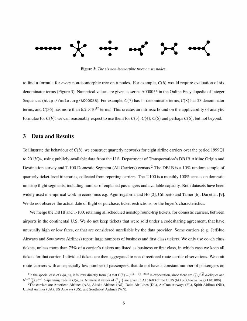
Figure 3: The six non-isomorphic trees on six nodes.

to find a formula for every non-isomorphic tree on b nodes. For example, C(6) would require evaluation of six

denominator terms (Figure 3). Numerical values are given as series A000055 in the Online Encyclopedia of Integer

Sequences (http://oeis.org/A000055). For example, C(7) has 11 denominator terms, C(8) has 23 denominator

terms, and C(36) has more than 6.2 ×1012 terms! This creates an intrinsic bound on the applicability of analytic

formulae for C(b): we can reasonably expect to use them for C(3), C(4), C(5) and perhaps C(6), but not beyond.1

3 Data and Results

To illustrate the behaviour of C(b), we construct quarterly networks for eight airline carriers over the period 1999Q1

to 2013Q4, using publicly-available data from the U.S. Department of Transportation’s DB1B Airline Origin and

Destination survey and T-100 Domestic Segment (All Carriers) census.2 The DB1B is a 10% random sample of

quarterly ticket-level itineraries, collected from reporting carriers. The T-100 is a monthly 100% census on domestic

nonstop flight segments, including number of enplaned passengers and available capacity. Both datasets have been

widely used in empirical work in economics e.g. Aguirregabiria and Ho [2], Ciliberto and Tamer [6], Dai et al. [9].

We do not observe the actual date of flight or purchase, ticket restrictions, or the buyer’s characteristics.

We merge the DB1B and T-100, retaining all scheduled nonstop round-trip tickets, for domestic carriers, between

airports in the continental U.S. We do not keep tickets that were sold under a codesharing agreement, that have

unusually high or low fares, or that are considered unreliable by the data provider. Some carriers (e.g. JetBlue

Airways and Southwest Airlines) report large numbers of business and first class tickets. We only use coach class

tickets, unless more than 75% of a carrier’s tickets are listed as business or first class, in which case we keep all

tickets for that carrier. Individual tickets are then aggregated to non-directional route-carrier observations. We omit

route-carriers with an especially low number of passengers, that do not have a constant number of passengers on

1In the special case of G(n, p), it follows directly from (3) that C(b) = p(b−1)(b−2)/2 in expectation, since there are(n

b)

p(b2) b-cliques and

bb−2 (nb)

pb−1 b-spanning trees in G(n, p). Numerical values of(b−1

2)

are given in A161680 of the OEIS (http://oeis.org/A161680).2The carriers are American Airlines (AA), Alaska Airlines (AS), Delta Air Lines (DL), AirTran Airways (FL), Spirit Airlines (NK),

United Airlines (UA), US Airways (US), and Southwest Airlines (WN).

6

each segment, or that are not present over the full sample period. In building the route networks, a node is an airport

that was served as a route origin or destination, and an edge is present if some passengers travelled on a direct route

between two nodes, for a given carrier-quarter. Our eight empirical networks are connected in every quarter of the

sample. Further details of the data treatment are available from the authors.

Since C(b) is intimately related to the relative number of cliques, we start by using the Bron-Kerbosch algorithm

to identify all cliques in a given network. Figure 4 displays the 2013Q4 network of Southwest Airlines, and highlights

one maximal 4-clique, between Albuquerque, Dallas, Houston, and Kansas City. It is interesting to see how many

maximal cliques of any given size there are in a network, and whether this distribution is stable over time. We

illustrate using Southwest’s network, in Figure 5, which shows that the distribution is more spread out, and that more

larger cliques appear, over time. There is a maximum clique size of eleven, which corresponds to 12.5% of all of the

airports served by Southwest in 2013Q4. This might seem surprising, given that Southwest’s network is relatively

sparse, with a density d(G) equal to 15% in that quarter. Since every airport in the maximum clique has at least

11 connections, we can think of it as a group of “important” airports, that are also very highly connected among

themselves.3 An operational reason for developing such groups could be to enable the opening of a large number

of new indirect routes between airport pairs, at relatively low cost, with the addition of a few well-chosen direct

routes. It seems likely that Southwest, through its network expansion, has focused both on increasing the size and

connectivity of a moderate number of “core” airports while also creating links from non-core airports into the core.4

Since there are a substantial number of cliques with more than three nodes, we examine how C(3), C(4) and

C(5) vary across carriers, and over time (Figure 8). We make the following remarks:

• There is considerable heterogeneity across carriers. For instance, Southwest has quite a stable C(3) over

1999Q1 to 2013Q4, despite its significant expansion in terms of airports and routes. On the other hand, United

has far more clustering (in triangles) from 2009 onwards, while Alaska has progressively less.

• Generalized clustering C(b) is highly positively correlated across b, for some networks e.g. Delta, and is also

positively correlated with network density (see Table 1 in Appendix B). Some of this follows by construction

e.g. for every newly formed 4-clique in a network, there will be between two and four new 3-cliques, while

every newly formed 5-clique will create between two and five new 4-cliques and between three and ten new

3We find evidence that nodes that belong to maximal cliques in Southwest’s network (a) are more connected, on average, than nodes thatare not in maximal cliques, and (b) that the average degree of nodes in maximal cliques increases in the order of the clique (Figure B.2).

4Not all networks evolve in this way e.g. the distribution of maximal cliques for American (AA) is far more stable over time (Figure B.3).

7

Figure 4: The Albuquerque–Dallas–Houston–Kansas City maximal 4-clique in Southwest’s network.

Figure 5: The distribution of maximal k-cliques in Southwest’s network, in 1999Q1, 2004Q2, 2009Q3 and 2013Q4.

8

Figure 6: Counterexample for C(3)≥C(4).

Figure 7: Counterexample for C(4)≥C(5).

3-cliques. High correlation reduces the information-content of C(4) and C(5), but it is unclear whether this

result holds for most classes of network, or if airline networks are in fact a special case. In order to control for

this correlation, we might consider performing the following regressions: C(4) = constant+β C(3)+ error

and C(5) = constant+β C(3)+γ C(4)+error, and using the residuals rather than C(4) and C(5) themselves.5

• There is some evidence that C(3)>C(4)>C(5), and we might think that this holds for all graphs. However,

we were able to construct a series of (pathological) counterexamples.

The general rule behind the construction is as follows: we create a complete Kb subgraph and then build a

“chain” of n−b nodes attached to one of the nodes in Kb. As n increases, the number of complete subgraphs

of order no more than b does not change (for instance, there are four triangles and one 4-complete subgraph in

Figure 6). Furthermore, increasing n after a certain point will only add paths of length b to the denominator of

C(b), and no other spanning trees (e.g. b-stars). It is easy to show that

C(3) =12

n+10; n≥ 5; C(4) =

16n+22

; n≥ 6, (6)

from which C(3)≥C(4) as n≤ 26, with equality when C(3) =C(4) = 13 .

5We illustrate the C(4) procedure in Figure B.1, for US Airways and Southwest (WN). Since C(3) and C(4) display evidence of a unitroot (US) and a unit root and trend (WN), we first run regressions of the form ∆C(b)t = α +δ t +u(b)t , for b = 3,4. We then regress thedifference and trend stationary u(4) on a constant and u(3), and find that 76% (US) and 89% (WN) of the variation in C(4) is “explained” byC(3). In this sense, C(4) is moderately informative once C(3) has been accounted for. It is unclear if other networks will give similar results.

9

In Figure 7, the number of 4-complete and 5-complete subgraphs is constant as n increases. Beyond a certain

point, only 4-paths and 5-paths are added to the denominators of C(4) and C(5) and no further 4-stars or

5-stars or 5-arrows are created. We can show that

C(4) =80

n+95; n≥ 7; C(5) =

125n+203

; n≥ 8, (7)

from which C(4) ≥C(5) as n ≤ 97. Equality occurs when C(4) = C(5) = 512 . Incidentally, for this graph,

C(3)≥C(4) as n≤ 12.2, i.e., n < 13. In principle, this construction can be used to show that C(b)<C(b+1)

for any b < n and sufficiently large n.

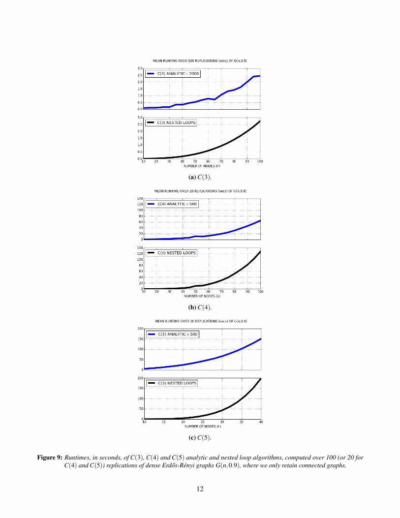
To end, we simulated the actual runtimes of the analytic formulae for C(b) for b = 3,4,5, on dense Erdos-Renyi

graphs G(n,0.9), and compared these with the runtimes of a simple nested loop implementation. We are able to

show that the theoretical asymptotic runtime of each of the analytic clustering formulae is lower than that of the

nested loops.6 However, the small-sample runtime is much lower when analytics are used (Figure 9): the analytic

algorithm is roughly 2,000 times faster for C(3) and more than 500 times faster for C(4) and C(5) for the dense

G(n, p). While analytic runtime gains are lower for sparse G(n, p), they remain very substantial, and this contributes

to making these generalized clustering coefficients a practical tool.

4 Conclusions

We have examined the nature and dynamics of topological cliques in real-world airline networks. We propose a

fast generalized clustering coefficient C(b), that can be readily implemented for b = 3,4,5. Despite some apparent

drawbacks, including the difficulty of deriving higher order C(b), and high correlation across different values of b,

the new measure can potentially provide insight regarding larger (than triangle) groups of completely-connected

nodes in a network. More generally, analytic formulae for subgraph enumeration might have application to other

statistics that are used in applied graph theory. Future work linking graphs and econometrics should lead to a better

understanding of the economic, strategic and spatial factors that drive dynamic clustering in real-world networks.

6The worst-case theoretical runtime of a nested loop implementation of C(b) is O(nb), since there are b nested loops. In a very sparsegraph, the actual runtime of nested loops can be much faster, and coding shortcuts can take advantage of the fact that not every b-tuple needsto be considered. Directly from (2), (4) and (5), we can see that the numerator will dominate the asymptotic runtime of the analytic formulae.We find that C(3) is O(nω ), C(4) is O(nω+1), and C(5) is O(nω+2), where ω is the exponent of matrix multiplication, for which currentimplementations give 2.38≤ ω ≤ 3. The very fast matrix multiplication algorithms due to Coppersmith and Winograd [8] and VassilevskaWilliams [25] both have ω ≈ 2.38, the well-known algorithm due to Strassen [24] has ω ≈ 2.81, and a naıve algorithm has ω = 3.

10

(a) Southwest Airlines. (b) American Airlines.

(c) US Airways. (d) United Airlines.

(e) Spirit Airlines. (f) AirTran Airways.

(g) Alaska Airlines. (h) Delta Air Lines.

Figure 8: The dynamic behaviour of C(3), C(4), C(5) and density from 1999Q1 to 2013Q4.

11

(a) C(3).

(b) C(4).

(c) C(5).

Figure 9: Runtimes, in seconds, of C(3), C(4) and C(5) analytic and nested loop algorithms, computed over 100 (or 20 forC(4) and C(5)) replications of dense Erdos-Renyi graphs G(n,0.9), where we only retain connected graphs.

12

References

[1] M. Agasse-Duval and S. Lawford. Subgraphs and motifs in a dynamic airline network. 2017. DEVI / ENACunpublished report.

[2] V. Aguirregabiria and C.-Y. Ho. A dynamic oligopoly game of the US airline industry: Estimation and policyexperiments. Journal of Econometrics, 168:156–173, 2012.

[3] F. Akbas, F. Meschke, and M.B. Wintoki. Director networks and informed traders. Journal of Accounting andEconomics, 62:1–23, 2016.

[4] A. Banerjee, A.G. Chandrasekhar, E. Duflo, and M.O. Jackson. The diffusion of microfinance. Science, 341:1236498, 2013.

[5] P. Baumgarten, R. Malina, and A. Lange. The impact of hubbing concentration on flight delays within airlinenetworks: An empirical analysis of the US domestic market. Transportation Research E, 66:103–114, 2014.

[6] F. Ciliberto and E. Tamer. Market structure and multiple equilibria in airline markets. Econometrica, 77:1791–1828, 2009.

[7] E. Cohen-Cole, A. Kirilenko, and E. Patacchini. Trading networks and liquidity provision. Journal of FinancialEconomics, 113:235–251, 2014.

[8] D. Coppersmith and S. Winograd. Matrix multiplication via arithmetic progressions. Journal of SymbolicComputation, 9:251–280, 1990.

[9] M. Dai, Q. Liu, and K. Serfes. Is the effect of competition on price dispersion non-monotonic? Evidence fromthe U.S. airline industry. Review of Economics and Statistics, 96:161–170, 2014.

[10] R. Diestel. Graph Theory. Springer, 5th edition, 2017.

[11] R. El-Khatib, K. Fogel, and T. Jandik. CEO network centrality and merger performance. Journal of FinancialEconomics, 116:349–382, 2015.

[12] R. Faris and D. Felmlee. Status struggles: Network centrality and gender segregation in same- and cross-genderaggression. American Sociological Review, 76:48–73, 2011.

[13] R. Guimera, S. Mossa, A. Turtschi, and L.A.N. Amaral. The worldwide air transportation network: Anomalouscentrality, community structure, and cities’ global roles. PNAS, 102:7794–7799, 2005.

[14] Y.V. Hochberg, A. Ljungqvist, and Y. Lu. Whom you know matters: Venture capital networks and investmentperformance. Journal of Finance, 62:251–301, 2007.

[15] M.O. Jackson. Social and Economic Networks. Princeton University Press, 2008.

[16] M.O. Jackson. Networks in the understanding of economic behaviors. Journal of Economic Perspectives, 28:3–22, 2014.

[17] D. Jungnickel. Graphs, Networks and Algorithms. Springer, 3rd edition, 2008.

[18] J. Lin and Y. Ban. The evolving network structure of US airline system during 1990-2010. Physica A, 410:302–312, 2014.

13

[19] O. Lordan, J.M. Sallan, and P. Simo. Study of the topology and robustness of airline route networks fromthe complex network approach: a survey and research agenda. Journal of Transport Geography, 37:112–120,2014.

[20] N. Movarraei and M.M. Shikare. On the number of paths of lengths 3 and 4 in a graph. International Journalof Applied Mathematical Research, 3:178–189, 2014.

[21] M.E.J. Newman. The structure and function of complex networks. SIAM Review, 45:167–256, 2003.

[22] D.T. Robinson and T.E. Stuart. Network effects in the governance of strategic alliances. Journal of Law,Economics, & Organization, 23:242–273, 2004.

[23] T. Ryczkowski, A. Fronczak, and P. Fronczak. How transfer flights shape the structure of the airline network.Scientific Reports, 7:5630, 2017.

[24] V. Strassen. Gaussian elimination is not optimal. Numerische Mathematik, 14:354–356, 1969.

[25] V. Vassilevska Williams. Multiplying matrices in O(n2.373) time. Mimeo, Available at: https://people.csail.mit.edu/virgi/matrixmult-f.pdf, 2014.

[26] T. Verma, N.A.M. Araujo, and H.J. Herrmann. Revealing the structure of the world airline network. ScientificReports, 4:5638, 2014.

[27] D.R. Wuellner, S. Roy, and R.M. D’Souza. Resilience and rewiring of the passenger airline networks in theUnited States. Physical Review E, 82:056101, 2010.

14

A Proofs

Derivations for the 3-star M(3)3 , the triangle M(3)

7 , the 4-star M(4)11 , the 4-path M(4)

13 , the tadpole M(4)15 , and the 4-

complete M(4)63 are given in Agasse-Duval and Lawford [1, Proposition II.1]. For completeness, we repeat them

here, without proof, in Proposition A.1. We also include the three spanning trees on five nodes: the 5-star M(5)75 , the

5-arrow M(5)77 and the 5-path M(5)

86 , and the 5-complete M(5)1023, all with their corresponding proofs.

Proposition A.1 (Analytic formulae for nested subgraph enumeration).

|M(3)3 |= ∑

i

(ki

2

)=

12 ∑

iki(ki−1). (8)

|M(3)7 |=

16

tr(g3). (9)

|M(4)11 |= ∑

i

(ki

3

)=

16 ∑

iki(ki−1)(ki−2). (10)

|M(4)13 |= ∑

(i, j)∈E(ki−1)(k j−1)−3 |M(3)

7 |. (11)

|M(4)15 |=

12 ∑

ki>2(g3)ii (ki−2). (12)

|M(4)63 |=

124 ∑

itr(g3

−i). (13)

|M(5)75 |= ∑

i

(ki

4

)=

124 ∑

iki(ki−1)(ki−2)(ki−3). (14)

|M(5)77 |= ∑

(i, j)?∈E

(ki−1

2

)(k j−1)−2|M(4)

15 |. (15)

|M(5)86 |=

12 ∑

i 6= j(g4)i j−2 |M(3)

3 |−9 |M(3)7 |−3 |M(4)

11 |−2 |M(4)13 |−2 |M(4)

15 |. (16)

15

|M(5)1023|=

15 ∑

i|M(4)

63 (g−i)|=1

120 ∑i

∑j∈ΓG(i)

tr(((g−i)− j)3). (17)

Remark A.1. In (13), g−i is the adjacency matrix corresponding to the subgraph induced by the neighbourhood

ΓG(i) of i, which we denote by G−i = (V (ΓG(i)),E(ΓG(i))), and we use (9) to count the number of triangles.

Remark A.2. In (15), ∑(i, j)∗∈E denotes summation over all edges in E, in both directions (i, j) and ( j, i).

Remark A.3. In (17), (g−i)− j is the adjacency matrix corresponding to the subgraph induced by the neighbourhood

ΓG−i( j) of j, which we denote by G−i− j = (V (ΓG−i( j)),E(ΓG−i( j))), and we use (13) to count the number of

4-cliques.

Proof of Proposition A.1. We treat each subgraph separately, and only report proofs that are not presented in

Agasse-Duval and Lawford [1, Proposition II.1].

(a) |M(5)75 |: Node i has edges to ki neighbours, and any four of those edges will form a 5-star, centered on i. The

result (14) follows immediately.

(b) |M(5)77 |: The method of proof is similar to that used for the count of the nested 4-path |M(4)

13 | in Agasse-Duval

and Lawford [1]. Consider any edge (i, j) ∈ E, as the central edge in a 5-arrow. Let i and j have degrees three

and two respectively, and let node i be directly-connected to nodes x and z, and let node j be directly-connected

to node y. Node i has ki−1 possible neighbours (for nodes x and z) and node j has k j−1 possible neighbours

(for node y). There are 12(ki− 1)(ki− 2)(k j− 1) ways in which two neighbours of i can be paired with a

neighbour of j, which gives a total of ∑(i, j)?∈E

(ki−1

2

)(k j− 1) across all possible central edges, in both

directions (we use (i, j)? to denote “(i, j) and ( j, i)”). This sum includes the unwanted cases x = y and x = z,

both of which form a tadpole. Since two of the four edges of the tadpole can be a candidate central edge (i, j)

of a 5-arrow, we subtract 2 |M(4)15 | to give result (15).

(c) |M(5)86 |: A very similar but less transparent proof can be found in Movarraei and Shikare [20]. A 5-path is a

walk of length 4 with no repeated nodes. Note that 12 ∑i6= j(g4)i j gives the number of walks of length 4 from i

to j, which does not only include 5-paths. There are five subgraphs in which we can find walks of length 4

that are not 5-paths:

16

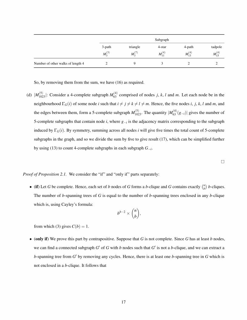
Subgraph

3-path triangle 4-star 4-path tadpole

M(3)3 M(7)

3 M(4)11 M(4)

13 M(4)15

Number of other walks of length 4 2 9 3 2 2

So, by removing them from the sum, we have (16) as required.

(d) |M(5)1023|: Consider a 4-complete subgraph M(4)

63 comprised of nodes j, k, l and m. Let each node be in the

neighbourhood ΓG(i) of some node i such that i 6= j 6= k 6= l 6= m. Hence, the five nodes i, j, k, l and m, and

the edges between them, form a 5-complete subgraph M(5)1023. The quantity |M(4)

63 (g−i)| gives the number of

5-complete subgraphs that contain node i, where g−i is the adjacency matrix corresponding to the subgraph

induced by ΓG(i). By symmetry, summing across all nodes i will give five times the total count of 5-complete

subgraphs in the graph, and so we divide the sum by five to give result (17), which can be simplified further

by using (13) to count 4-complete subgraphs in each subgraph G−i.

Proof of Proposition 2.1. We consider the “if” and “only if” parts separately:

• (if) Let G be complete. Hence, each set of b nodes of G forms a b-clique and G contains exactly(n

b

)b-cliques.

The number of b-spanning trees of G is equal to the number of b-spanning trees enclosed in any b-clique

which is, using Cayley’s formula:

bb−2 ×(

nb

),

from which (3) gives C(b) = 1.

• (only if) We prove this part by contrapositive. Suppose that G is not complete. Since G has at least b nodes,

we can find a connected subgraph G′ of G with b nodes such that G′ is not a b-clique, and we can extract a

b-spanning tree from G′ by removing any cycles. Hence, there is at least one b-spanning tree in G which is

not enclosed in a b-clique. It follows that

17

number of b-spanning trees in G≥ number of b-spanning trees enclosed in a b-clique+1

> number of b-spanning trees enclosed in a b-clique

= bb−2×number of b-cliques in G,

and so C(b)< 1 from (3), which proves the proposition.

18

B Additional Figures and Tables

Variable C(3) C(4) C(5) densityC(3) 1.000 0.394 −0.012 0.790p-value 0.000 0.002 0.927 0.000C(4) - 1.000 0.910 0.365p-value - 0.000 0.000 0.004C(5) - - 1.000 0.039p-value - - 0.000 0.766density - - - 1.000p-value - - - 0.000

(a) Southwest Airlines.

Variable C(3) C(4) C(5) densityC(3) 1.000 0.992 0.963 0.864p-value 0.000 0.000 0.000 0.000C(4) - 1.000 0.984 0.852p-value - 0.000 0.000 0.000C(5) - - 1.000 0.861p-value - - 0.000 0.000density - - - 1.000p-value - - - 0.000

(b) American Airlines.

Variable C(3) C(4) C(5) densityC(3) 1.000 0.897 0.659 0.781p-value 0.000 0.000 0.000 0.000C(4) - 1.000 0.916 0.459p-value - 0.000 0.000 0.000C(5) - - 1.000 0.102p-value - - 0.000 0.438density - - - 1.000p-value - - - 0.000

(c) US Airways.

Variable C(3) C(4) C(5) densityC(3) 1.000 0.994 0.968 0.965p-value 0.000 0.000 0.000 0.000C(4) - 1.000 0.989 0.936p-value - 0.000 0.000 0.000C(5) - - 1.000 0.887p-value - - 0.000 0.000density - - - 1.000p-value - - - 0.000

(d) United Airlines.

Variable C(3) C(4) C(5) densityC(3) 1.000 0.844 0.439 −0.256p-value 0.000 0.000 0.000 0.049C(4) - 1.000 0.709 −0.414p-value - 0.000 0.000 0.001C(5) - - 1.000 −0.450p-value - - 0.000 0.000density - - - 1.000p-value - - - 0.000

(e) Spirit Airlines.

Variable C(3) C(4) C(5) densityC(3) 1.000 0.854 0.333 0.539p-value 0.000 0.000 0.009 0.000C(4) - 1.000 0.682 0.156p-value - 0.000 0.000 0.235C(5) - - 1.000 −0.255p-value - - 0.000 0.049density - - - 1.000p-value - - - 0.000

(f) AirTran Airways.

Variable C(3) C(4) C(5) densityC(3) 1.000 NA NA 0.840p-value 0.000 NA NA 0.000C(4) - 1.000 NA NAp-value - 0.000 NA NAC(5) - - 1.000 NAp-value - - 0.000 NAdensity - - - 1.000p-value - - - 0.000

(g) Alaska Airlines.

Variable C(3) C(4) C(5) densityC(3) 1.000 0.970 0.807 0.838p-value 0.000 0.000 0.000 0.000C(4) - 1.000 0.919 0.743p-value - 0.000 0.000 0.000C(5) - - 1.000 0.488p-value - - 0.000 0.000density - - - 1.000p-value - - - 0.000

(h) Delta Air Lines.

Table 1: Pearson’s correlation test for C(3), C(4), C(5) and density for different networks.

19

(a) US Airways.

(b) Southwest Airlines.

Figure B.1: Regression of C(4)? on a constant and C(3)?, where the star notation indicates that both coefficients have beencorrected so that they are difference and trend stationary, before performing the regression (see footnote 5).

20

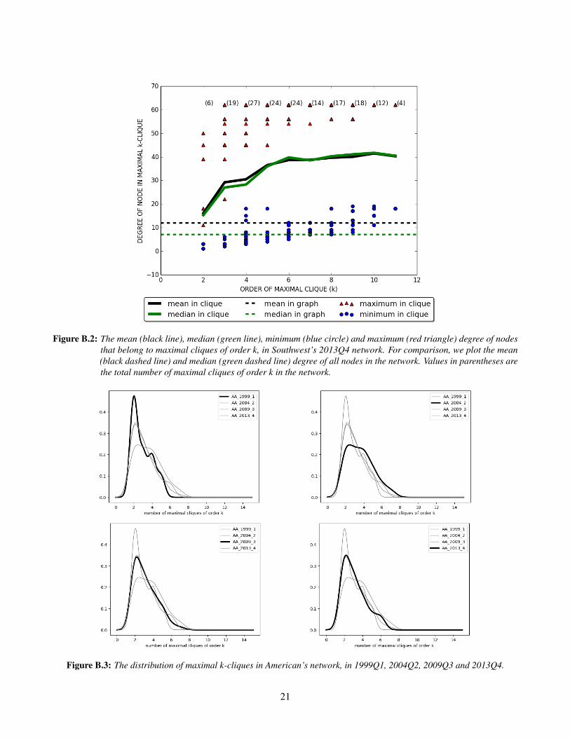
Figure B.2: The mean (black line), median (green line), minimum (blue circle) and maximum (red triangle) degree of nodesthat belong to maximal cliques of order k, in Southwest’s 2013Q4 network. For comparison, we plot the mean(black dashed line) and median (green dashed line) degree of all nodes in the network. Values in parentheses arethe total number of maximal cliques of order k in the network.

Figure B.3: The distribution of maximal k-cliques in American’s network, in 1999Q1, 2004Q2, 2009Q3 and 2013Q4.

21